CREDIT RATINGS CONSERVATISM AND EARNINGS …credit ratings conservatism and earnings management a dissertation submitted to the graduate division of the university of hawai‘i at

CREDIT RATINGS CONSERVATISM AND EARNINGS MANAGEMENT

A DISSERTATION SUBMITTED TO THE GRADUATE DIVISION OF THE

UNIVERSITY OF HAWAI‘I AT MĀNOA IN PARTIAL FULFILLMENT OF THE

REQUIREMENTS FOR THE DEGREE OF

DOCTOR OF PHILOSOPHY

IN

BUSINESS ADMINISTRATION

AUGUST 2017

By

Kunsu Park

Dissertation Committee:

Jian Zhou, Chairperson

S. Ghon Rhee

John Wendell

Liming Guan

Inessa Love

Keywords: Credit Ratings Conservatism, Earnings Management

ii

DEDICATION

I dedicate this dissertation to my family. A very special dedication goes to my

parents, Jongoh Park and Jeongkeun Oh, who always encourage me to pursue this study

and to continue my education in the fields of economics, management and administrative

science (MAS), finance and accounting. My parents always give me unconditional love

and support. I would like to dedicate this work to my first younger sister Kyeongok Park,

brother-in-law Kitae Hong, and two nephews Hayoon Hong and Haram Hong, for their

unwavering love and support. I would also like to dedicate this work to my second

younger sister Kyungja Park, brother-in-law Wooseong Jin, and two nephews Jonghwa

Jin and Jonghyun Jin, for their constant love and support.

iii

ACKNOWLEDGEMENTS

I would like to thank all my committee members, Dr. Jian Zhou, Dr. S. Ghon

Rhee, Dr. John Wendell, Dr. Liming Guan, and Dr. Inessa Love, for their valuable

comments and inspiring discussions, and continued guidance. In particular, my

dissertation advisor Dr. Jian Zhou has always given me plenty of advice, support, and

encouragement during my Ph.D. studies. I would also like to express my deepest

gratitude and special thanks to Dr. S. Ghon Rhee for his continued support, inspiration,

guidance, and encouragement throughout the journey of this dissertation. He has been an

exceptional academic mentor to me. Without their support and guidance, I would not

have been able to complete this dissertation.

I would also like to thank Dr. Boochun Jung, Dr. Shirley Daniel, Dr. Hamid

Pourjalali, Dr. David Yang, Dr. Tom Pearson, Dr. Roger Debreceny, Dr. Wei Huang, Dr.

Qianqiu Liu, Dr. Sang-Hyop Lee, Dr. Song K. Choi, and Dr. Kentaro Hayashi for their

support, encouragement, and kind assistance during my Ph.D. studies. In particular, Dr.

Song K. Choi has given me invaluable advice and support through all stages of my work.

Dr. Boochun Jung always gives me valuable comments and suggestions regarding my

work. I would like to acknowledge Dr. Mark Anderson, who encouraged me to pursue

my Ph.D. studies in the field of accounting.

I would like to express my appreciation to my Ph.D. colleagues for their

continued support and motivation. Among those who deserve special recognition are

iv

James Youn, Cheol-Rin Park, Jaeseong Lim, Jaisang Kim, Youngbin Kim, and Jin Suk

Park. I also want to express my thanks to my friends for their encouragement and

unconditional love. Those who deserve special thanks are Kyung Sung Jung, Young

Kwark, Jongmin Kim, Tong Hyouk Kang, Soonchul Hyun, Joo Hyung Lee, Jangho Gil,

Jong-Min Oh, Seong K. Byun, Sung Hoon Woo, YoungJae Kim, Hojin Jung, Minwoo

Lee, Sang Baum Solomon Kang, Sung Bok Lee, Jason Shin, Hyunsuk Jang, Chris Choi,

Dong Wook Huh, Kwondo Song, and Soonsup Hong.

I would also like to acknowledge Nicole Kurashige and Avree Ito-fujita for their

assistance and guidance in helping me to improve English writing skills during my Ph.D.

studies. I would like to thank Rosemarie Woodruff and Adam Pang for your continued

encouragement and assistance. I would also like to thank Bumhwan Jeon, Kara

Youngshim Bang, and Dawna Kim for unconditionally supporting me throughout my

studies.

Last but not least, I would like to thank Dr. Young Mok Choi and Dr. Se Hun Lim

for their motivation, support, and assistance during my studies.

v

ABSTRACT

I examine whether ratings conservatism influences a firm’s earnings management.

First, total earnings management, calculated as the sum of real and accrual-based

earnings management measures, increases in response to ratings conservatism. Ratings

conservatism leads to a substitution between real and accrual-based earnings

management, indicating that the increase in real earnings management is greater than the

decrease in accrual-based earnings management. Next, the negative relation between

ratings conservatism and accrual-based earnings management is more pronounced for

firms with low credit quality than for those with high credit quality. However, the

positive relation between ratings conservatism and real earnings management does not

apply to both investment- and speculative-grade firms. The results are robust to sample

selection bias, alternative measures of accrual-based earnings management, alternative

industry classifications, alternative cut-off years employed when measuring ratings

conservatism, the effect of external events, omitted variable bias, and different

specifications for ratings models. In addition, there is no evidence of earnings smoothing

and asymmetric timeliness loss recognition relating to ratings conservatism. Overall, this

study finds that ratings conservatism affects a firm’s incentive to manage its reported

earnings. This study also represents the first step towards understanding how ratings

conservatism influences the earnings management behaviors of managers.

vi

TABLE OF CONTENTS

DEDICATION................................................................................................................... ii

ACKNOWLEDGEMENTS ............................................................................................ iii

ABSTRACT ....................................................................................................................... v

LIST OF TABLES ........................................................................................................... ix

LIST OF FIGURES ....................................................................................................... xiii

INTRODUCTION ..................................................................................... 1 CHAPTER 1

RELATED LITERATURE AND HYPOTHESES DEVELOPMENTCHAPTER 2

............................................................................................................................... 13

2.1 Credit Ratings and Earnings Management .............................................................. 13

2.2 Stringent Trends in Rating Standards (“Ratings Conservatism”) ........................... 16

2.3 Ratings Conservatism and Earnings Management .................................................. 18

RESEARCH DESIGN ............................................................................ 28 CHAPTER 3

3.1 Measuring Credit Ratings Conservatism ................................................................. 28

3.2 Measures of Earnings Management ........................................................................ 31

3.2.1 Accrual-Based Earnings Management (AEM) ............................................. 31

3.2.2 Real Earnings Management (REM) .............................................................. 32

3.2.3 Total Earnings Management (TEM) ............................................................. 35

3.3 Baseline Regression Model ..................................................................................... 35

vii

SAMPLE SELECTION AND ESTIMATION OF RATINGS CHAPTER 4

MODELS ............................................................................................................. 41

4.1 Data Selection ......................................................................................................... 41

4.2 Ratings Models ........................................................................................................ 42

4.2.1 Data Description ............................................................................................ 42

4.2.2 Estimating Ratings Models ........................................................................... 42

RESULTS ................................................................................................. 44 CHAPTER 5

5.1 Descriptive Statistics and Correlations ................................................................... 44

5.2 Relation between Ratings Conservatism and Accrual-Based Earnings Management:

Testing H1 ......................................................................................................................... 46

5.3 Relation between Ratings Conservatism and Real Earnings Management: Testing

H1 50

5.4 Relation between Ratings Conservatism and Total Earnings Management ........... 53

5.5 Investment- and Speculative-Grade Firms (Accrual-Based Earnings Management):

Testing H2 ......................................................................................................................... 54

5.6 Investment- and Speculative-Grade Firms (Real earnings management): Testing H2

58

POTENTIAL SAMPLE SELECTION BIAS ....................................... 61 CHAPTER 6

ADDITIONAL ANALYSES ................................................................... 63 CHAPTER 7

7.1 Ratings Conservatism and Earnings Smoothing (EM_SMOOTH) ......................... 63

7.2 Ratings Conservatism and Asymmetric Timely Loss Recognition ........................ 67

viii

ROBUSTNESS TESTS ........................................................................... 73 CHAPTER 8

8.1 Alternative Measures of Accrual-Based Earnings Management ............................ 73

8.2 Using Alternative Industry Classifications When Calculating Ratings Conservatism

and Earnings Management Proxies ................................................................................... 77

8.3 Alternative Cut-Off Years Employed When Measuring Ratings Conservatism ..... 79

8.4 Controlling for the Effect of the Global Financial Crisis of 2007-2008 ................. 80

8.5 Possibility of Omitted Variable Bias ....................................................................... 81

8.6 Re-estimation of the Regression Equation (8) ........................................................ 82

8.7 Validity of the Ratings Model ................................................................................. 83

8.8 Role of Accounting Quality in the Assignment of Credit Ratings .......................... 84

CONCLUSION ........................................................................................ 86 CHAPTER 9

LIMITATIONS AND FUTURE RESEARCH ................................... 88 CHAPTER 10

APPENDIX A VARIABLE DEFINITIONS: RATINGS MODEL ............................ 90

APPENDIX B VARIABLE DEFINITIONS: BASELINE REGRESSION MODEL91

APPENDIX C MEASURE OF ASYMMETRIC TIMELY LOSS RECOGNITION:

Khan and Watts’ C_Score (2009, p. 136) .......................................................... 96

REFERENCES .............................................................................................................. 158

ix

LIST OF TABLES

Table 1 Number of Firms by S&P Credit Ratings Categories and Year, 1985-2014

(CHAPTER 4) ........................................................................................................... 97

Table 2 Summary Statistics for Relevant Variables used in Ratings Models

(CHAPTER 4) ........................................................................................................... 98

Table 3 Ratings Models (CHAPTER 4) ....................................................................... 99

Table 4 Descriptive Statistics (CHAPTER 5) ............................................................. 102

Table 5 Pearson Correlation Coefficients (CHAPTER 5) .......................................... 103

Table 6 Relation between Ratings Conservatism and Accrual-Based Earnings

Management (Testing H1 using the ratings conservatism measure, Rat_Diff_Firm)

(CHAPTER 5) ......................................................................................................... 104

Table 7 Relation between Ratings Conservatism and Accrual-Based Earnings

Management (Testing H1 using the ratings conservatism measure, Rat_Diff_Ind)

(CHAPTER 5) ......................................................................................................... 106

Table 8 Relation between Ratings Conservatism and Real Earnings Management

(Testing H1 using the ratings conservatism measure, Rat_Diff_Firm) (CHAPTER 5)

................................................................................................................................. 108


(Testing H1 using the ratings conservatism measure, Rat_Diff_Ind) (CHAPTER 5)

................................................................................................................................. 110

x

Table 10 Relation between Ratings Conservatism and Total Earnings Management

(Testing H1 using TEM1) (CHAPTER 5) ............................................................... 112


(Testing H1 using TEM2) (CHAPTER 5) ............................................................... 114

Table 12 Investment- Grade (IG) and Speculative-Grade (SG) Firms


................................................................................................................................. 116



................................................................................................................................. 118


(Testing H2 using REM1) (CHAPTER 5) ............................................................... 120


(Testing H2 using REM2) (CHAPTER 5) ............................................................... 122

Table 16 Potential Sample Selection Bias


................................................................................................................................. 124

Table 17 Additional Analysis

Relation between Ratings Conservatism and Earnings Smoothing (CHAPTER 7) 127

xi


Relation between Ratings Conservatism and Asymmetric Timely Loss Recognition

(CHAPTER 7) ......................................................................................................... 129

Table 19

Alternative Measures of Accrual-Based Earnings Management 1: Testing H1

(CHAPTER 8) ......................................................................................................... 130

Table 20


(CHAPTER 8) ......................................................................................................... 133

Table 21


(CHAPTER 8) ......................................................................................................... 136

Table 22


(CHAPTER 8) ......................................................................................................... 139

Table 23

Using a Three-Digit SIC Industry: Testing H1 (CHAPTER 8) ............................... 142

Table 24

Alternative Cut-Off Years (1985-1997): Testing H1 (CHAPTER 8) ..................... 145

Table 25

Alternative Cut-Off Years (1985-1998): Testing H1 (CHAPTER 8) ..................... 148

xii

Table 26

Controlling for the Effect of Global Financial Crisis of 2007-2008: Testing H1

(CHAPTER 8) ......................................................................................................... 151

Table 27

Controlling for the Controlling for Additional Variables: Testing H1 (CHAPTER 8)

................................................................................................................................. 154

xiii

LIST OF FIGURES

Figure 1 Plot of Coefficient on Year Dummies in Ratings Models (CHAPTER 4) ... 157

1

CHAPTER 1

INTRODUCTION

Over the past three decades, credit ratings of U.S. firms, on average, have declined. Prior

research documents that the downward trend in credit ratings is attributed to more stringent credit

standards by credit ratings agencies (Blume et al., 1998; Alp, 2013; Baghai et al., 2014; Afik et al.,

2016).1 The term “ratings conservatism” refers to the tendency for credit ratings agencies

to tighten their credit standards over time. Several studies focus on a firm’s earnings

management in relation to credit ratings and to credit ratings changes (Ali and Zhang, 2008; Alissa

et al., 2013; Jung et al., 2013; Kim et al., 2013; Shen and Huang, 2013). However, the relation

between ratings conservatism and earnings management has yet to be investigated. My study

begins with the following research questions: Does ratings conservatism affect a firm’s earnings

management behavior? If so, does ratings conservatism influence the choice between real and

accrual-based earnings management? In addition to real and accrual-based earnings management,

does ratings conservatism affect other types of earnings management, such as earnings smoothing

and asymmetric timeliness loss recognition? To answer these questions, I examine how ratings

conservatism influences a firm’s incentive to manage its reported earnings through earnings

1 An exception is Jorion et al. (2009), who argue that the downward trend in corporate credit ratings is

due to the decline in accounting quality over time. On the other hand, my study is based on the argument by

previous studies that the decline in credit ratings is primarily caused by the tightening rating standards

applied by ratings agencies (Blume et al., 1998; Alp, 2013; Baghai et al., 2014; Afik et al., 2016). I focus

on the impact of stringent rating standards over time (“ratings conservatism”) on a firm’s earnings

management. I do not, however, explore why bond ratings of U.S. firms have declined over time. To do

this, I first replicate Baghai et al.’s (2014) findings. I then extend the sample period to 2014 and calculate

ratings conservatism proxies proposed by Baghai et al. (2014). Finally, I investigate whether ratings

conservatism influences a firm’s incentive to manage earnings via earnings management.

2

management.

Issues concerning a firm’s earnings management have attracted much interest from

academics and practitioners over several decades.2 Prior literature investigates potential motives for

a firm’s earnings management from different perspectives, such as management compensation

contracts (Healy, 1985; Dechow and Sloan, 1991; Gaver et al., 1995; Hothausen et al., 1995;

Balsam, 1998; Guidry et al., 1999), lending contracts (Watts and Zimmerman, 1986; DeFond and

Jiambalvo, 1994), regulatory motives (Moyer, 1990; Collins et al., 1995), political costs (Watts and

Zimmerman, 1986; Jones, 1991), capital market motives (Teoh et al., 1998a, 1998b), and so on. In

addition to these motives, three recent studies (Ali and Zhang, 2008; Alissa et al., 2013; Kim et al.,

2013) provide an additional incentive for managers to manage their firms’ earnings in the context of

credit ratings and credit ratings changes. Managers are more likely to behave opportunistically.

Specifically, earnings management behaviors in response to credit ratings and credit ratings changes

can affect a firm’s cost of capital and further its stock price. Therefore, credit ratings are one of the

important characteristics that explain a firm’s earnings management behaviors.

Prior research also shows that credit ratings agencies have become more conservative with

their credit standards and provides the testable implications of ratings conservatism for researchers

and managers (Blume et al., 1998; Alp, 2013; Baghai et al., 2014; Afik et al., 2016). One may take

into account ratings conservatism in examining a potential motive for a firm’s earnings

2 Schipper (1989) states earnings management as “a purposeful intervention in the external financial

reporting process, with the intent of obtaining some private gain (as opposed to, say, merely facilitating the

neutral operation of the process)” (p. 92). In a similar way, as described by Healy and Wahlen (1999),

“Earnings management occurs when managers use judgment in financial reporting and in structuring

transactions to alter financial reports to either mislead some stakeholders about the underlying economic

performance of the company or to influence contractual outcomes that depend on reported accounting

numbers” (p. 368).

3

management in the framework of credit ratings. This is indeed what I explore in this paper.

Corporate credit ratings are determined by not only a firm’s financial conditions and operating

performance at a current point in time, but also by ratings agencies’ evaluation criteria or standards.

If the tightening of credit standards by ratings agencies remains persistent over time, such stringent

standards influence the opportunistic earnings management behaviors of managers.

I propose two hypotheses to examine the relation between ratings conservatism and

earnings management. The first hypothesis is: Credit ratings conservatism leads to a substitution

between real and accrual-based earnings management. My hypothesis of the substitution between

real and accrual-based earnings management is based on theoretical, empirical, and anecdotal

evidence.3 Managers use real and accrual-based earnings management either individually or jointly

to achieve one or more objectives (Kothari et al., 2016). I infer that firms pursue alternate means to

manage their reported earnings in response to ratings conservatism. Mangers have incentives to

manage their firms’ reported earnings via real earnings management to meet earnings targets

(Roychowdhury, 2006). Managers in firms more affected by stringent rating standards engage in

real earnings management to meet or beat earnings benchmarks in an attempt to enhance their

credibility with capital markets and to achieve desired credit ratings. For example, survey evidence

provided by Graham et al. (2005) shows that the chief financial officers (CFOs) responded that their

firms try to meet earnings benchmarks in an effort to “achieve or preserve a desired credit rating.”

(p. 25). Firms affected by ratings conservatism engage in more real earnings management and gain

3 Blume et al. (1998), Graham and Harvey (2001), Bartov et al. (2002), Graham et al. (2005),

Ashbaugh-Skaife et al. (2006), Kisgen (2006), Cohen et al. (2008), Jorion et al. (2009), Cohen and Zarowin

(2010), Gunny (2010), Caton et al. (2011), Zang (2012), Shen and Huang (2013), Baghai et al. (2014), Ge

and Kim (2014), and Standard & Poor's (2008, 2015) contribute to the study of this topic. Please see

subsection 2.3 for more details.

4

better credit ratings by meeting earnings benchmarks, which consequently access debt markets at a

more favorable rate.4 Thus, firms that suffer more from ratings conservatism engage in more real

earnings management. On the other hand, I predict that ratings conservatism restrains managers

from engaging in accrual-based earnings management because high accounting accruals are

observable to sophisticated credit rating agencies as well as regulators, auditors and even

institutional investors (Cohen et al., 2008; Dechow et al., 2010; Zang, 2012; Chan et al., 2015).

Firms with high accounting accruals are subject to closer scrutiny from regulators (the SEC),

auditors, and even credit rating agencies. High accounting accruals are more likely to be related to

accrual-based earnings management, which results in a decrease in financial reporting quality and

thus an increase in uncertainty among capital market participants, including credit rating agencies

(Akins, 2017). The high accounting accruals can impede credit ratings agencies from timely and

accurately assigning credit ratings to firms and have a negative influence on a firm’s future credit

ratings (Ashbaugh-Skaife et al., 2006; Jorion et al., 2009; Caton et al., 2011; Bae et al., 2013; Shen

and Huang, 2013; Standard & Poor’s, 2015).5 Accordingly, high accounting accruals are negatively

associated with the assignment of credit ratings by ratings agencies, which likely result in tighter

rating standards. Thus, firms more affected by ratings conservatism have incentives to engage in

less accrual-based earnings management. Collectively, as ratings conservatism increases, real

4 See, for example, Bartov et al. (2002) and Gunny (2010).

5 Based on these prior studies, I infer that credit rating agencies are able to (fully) comprehend a firm’s

accounting accruals process and penalize earnings management behaviors of managers. For example,

Standard & Poor’s (2015) states that accounting quality is considered to be a factor in the process of

assigning bond ratings.

5

earnings management increases while accrual-based earnings management decreases.6 Another

possible explanation for the substitution between real and accrual-based earnings management in

response to ratings conservatism is as follows: Ratings conservatism implies that ratings agencies

apply more stringent requirements (or criteria) on qualitative information (accounting quality) as

well as on quantitative information (past audited financial statements) in their assignment of credit

ratings. Ratings conservatism also implies that, given that financial conditions or operating

performance are comparable with the previous year, firms affected more by ratings conservatism

receive relatively worse ratings than before. Accordingly, due to their ratings disadvantages, firms

experience difficulty in obtaining debt financing, which could lead to lower levels of debt.7

Consequently, firms would deviate from their target debt (or target leverage) ratios. To make up for

the deviation, the firms attempt to revert back to their target debt ratios. These firms have a desire to

improve their credit ratings because improved ratings can signal a lower likelihood of credit risk (or

default risk) to market participants, including investors and creditors, which likely results in lower

debt financing costs. Therefore, in response to ratings conservatism, managers have incentives to

improve their accounting quality (or earnings quality) by engaging in less accrual-based earnings

management in an attempt to achieve desirable or better credit ratings. In other words, these firms

engage in less accrual-based earnings management to improve accounting quality for a better credit

rating to access debt markets at a favorable rate. On the other hand, ratings conservatism can lead

managers to resort real earnings management, which possibly benefits from an increase in earnings

6 Of course, it is possible that firms use the combination of real and accrual-based earnings

management. 7 If capital markets completely take into account the effect of ratings conservatism, firms would not

need to consider it in their debt financing decisions.

6

and thus positively affects debt ratings in spite of its costs.8 In a circumstance that rating agencies

have become more conservative in their assignment of credit ratings, the costs of real earnings

management (e.g., lower subsequent operating performance (Gunny, 2005)) are be less than its

benefits (e.g., the benefits from beating or meeting earnings targets/benchmarks (Graham et al.,

2005; Gunny, 2010; Zang, 2012)) as discussed earlier.9 Taken together, in response to ratings

conservatism, mangers prefer real earnings management to accrual-based earnings management.

The second hypothesis is: The positive (negative) relation between ratings conservatism and real

earnings management (accrual-based earnings management) is more pronounced for firms with

low credit quality than for those with high credit quality. Given that credit ratings agencies consider

accounting quality as an important item for their assignment of credit ratings, I infer that to obtain

better credit ratings and thus access debt markets at a more favorable rate, firms with low credit

quality, i.e., speculative-grade firms, have more (less) incentive to manage their reported earnings

via real earnings management (accrual-based earnings management) than those with high credit

quality, i.e., investment-grade firms.

Using a sample of publicly traded and rated U.S. firms between 1985 and 2014, I

investigate the relation between ratings conservatism and earnings management. I use the

absolute value of discretionary accruals (ABS_DA) as well as positive and negative

discretionary accruals as a proxy for a firm’s accrual-based earnings management. To

calculate discretionary accruals, I follow Dechow et al. (1995) and use the cross-sectional

8 See, for example, Ewert and Wagenhofer (2005).

9 Graham et al. (2005) provide survey evidence on why chief financial officers (CFOs) have a desire to

meet or beat earnings benchmarks. Please see Graham et al. (2005, p. 21-43) for more details.

7

modified Jones (1991) model. Next, following Roychowdhury (2006), I estimate the

abnormal levels of operating cash flows, production costs and discretionary expenditures

to capture a firm’s real earnings management. To capture total real earnings management,

I follow Cohen et al. (2008), Cohen and Zarowin (2010) and Zang (2012), and generate

two alternative measures, REM1 (calculated as the sum of the abnormal level of

discretionary expenses multiplied by negative one and the abnormal level of production

costs) and REM2 (computed as the sum of the abnormal level of discretionary expenses

and the abnormal level of operating cash flows, both multiplied by negative one).

Furthermore, to examine the effect of ratings conservatism on overall earnings

management, I follow Chan et al. (2015) and generate two measures, TEM1 (calculated

as the sum of the signed discretionary accruals (DA) and the aggregate real earnings

management (REM1)) and TEM2 (computed as the sum of the signed discretionary

accruals (DA) and the aggregate real earnings management (REM2)).10

On the other hand,

I employ two measures of credit ratings conservatism developed by Baghai et al. (2014).

The procedures for measuring ratings conservatism are similar to those in Baghai et al.

(2014). Specifically, in the first step, I estimate ratings models between 1985 and 1996 to

predict ratings between 1997 and 2014. In the second step, I obtain two ratings

conservatism proxies, measured as the difference between a firm’s actual and predicted

ratings.

Consistent with the first hypothesis, I find that ratings conservatism is negatively

10

Furthermore, for additional analyses, I use earnings smoothing measures and asymmetric timely loss

recognition measures. See subsections 6.1 and 6.2 for more details.

8

related to accrual-based earnings management, measured through the absolute value of

discretionary accruals and positive discretionary actuals. These findings suggest that

firms affected more by ratings conservatism engage in less accrual-based earnings

management and income-increasing earnings management.11

Furthermore, with respect to

negative discretionary accruals, I find a positive relation between ratings conservatism

and accrual-based earnings management. This finding indicates that firms affected more

by ratings conservatism engage in less income-decreasing earnings management. Taken

together, my evidence suggests that accrual-based earnings management decreases with

ratings conservatism. In contrast, I find that firms affected more by ratings conservatism

engage in more real earnings management, measured as the abnormal levels of production costs,

discretionary expenses, and cash flow from operations as well as aggregate measures of real

earnings management, REM1 and REM2. These findings support my first hypothesis. To

summarize, ratings conservatism leads to a substitution between real and accrual-based earnings

management. Furthermore, given the two opposite effects, I find that ratings conservatism increases

total earnings management. This finding implies that the increase in real earnings management is

greater than the decrease in accrual-based earnings management. Next, consistent with my

second hypothesis, I find that the negative relation between ratings conservatism and

accrual-based earnings management (measured as the absolute value of discretionary

accruals) is stronger for speculative-grade firms than for investment-grade firms.

However, I find that the positive relation between ratings conservatism and real earnings

11

When using the ratings conservatism measure based on firm fixed effects, I find no evidence of

income-increasing earnings management.

9

management does not apply to both investment- and speculative-grade firms. This finding is

inconsistent with my hypothesis that the positive relation is more pronounced for speculative-grade

firms than for speculative-grade firms. With respect to a series of robustness checks, my main

results are robust to sample selection bias, alternative measures of accrual-based earnings

management, alternative industry classifications, alternative cut-off years employed when

measuring ratings conservatism, the effect of external events, omitted variable bias, and

different specifications for ratings models. Finally, regarding additional analyses, I find no

evidence that firms more affected by ratings conservatism tend to engage in more or less earnings

smoothing. I also find inconsistent results regarding the relation between ratings conservatism and

each measure of asymmetric timeliness loss recognition.

My study provides the following several contributions: First, this study contributes to the

literature on ratings conservatism by providing evidence that the tightening of rating standards

affects a firm’s earnings management. Until now, there is little literature on the downward trend in

corporate credit ratings of U.S. firms over time (Blume et al., 1998; Jorion et al., 2009; Alp, 2013;

Baghai et al., 2014; Afik et al., 2016). These studies document that rating standards have become

more stringent over the past decades, except for Jorion et al. (2009). Specifically, Blume et al. (1998)

argue that corporate credit ratings have become more stringent for the period of 1978 to 1995. Their

argument is supported by subsequent studies, including Alp (2013), Baghai et al. (2014), and Afik

et al. (2016). In contrast, Jorion et al. (2009) claim that the tightening of rating standards only

applies to investment-grade firms, suggesting that the downward trend in credit ratings is mainly

due to the change in accounting quality over time, not stringent rating standards by ratings agencies .

10

Unlike Jorion et al. (2009) and Alp (2013), Baghai et al. (2014) develop a measure of ratings

conservatism and further examine whether ratings conservatism affects corporate behaviors, such as

a firm’s capital structure decisions, cash holdings, and debt spreads. I further extend prior studies,

especially Baghai et al.’s (2014), by considering whether ratings conservatism can affect a firm’s

earnings management. This study provides evidence that firms take on different earnings

management strategies in response to ratings conservatism.

Second, this study extends prior literature on the relation between credit ratings (changes)

and earnings management by examining the effect of ratings conservatism on a firm’s earnings

management. Among prior studies (Ali and Zhang, 2008; Alissa et al., 2013; Kim et al., 2013),

Alissa et al. (2013) examine how a manager’s discretion of earnings management affects credit

ratings. They document that when a firm’s current ratings are below (above) expected ratings, the

firm has an incentive to manage its reported earnings upward (downward). My study is, however,

different from theirs in several ways. First, unlike Alissa et al., I examine how ratings conservatism

affects earnings management using a novel measure of ratings conservatism developed by Baghai

et al. (2014). Second, my study takes into account the behaviors of credit ratings agencies using a

measure of ratings conservatism. This study provides evidence that ratings conservatism can be one

of the potential characteristics that affect a firm’s earnings management. Although there are prior

studies on earnings management from the perspectives of credit ratings (change), there is no

evidence of whether the tightening of rating standards by credit ratings agencies influences a firm’s

earnings management. With my study, I hope to fill this gap by providing the impact of ratings

conservatism on earnings management. My study is different from prior literature on the relation

11

between credit ratings (changes) and earnings management in that I take into account both the

opportunistic behaviors of managers and the behavioral changes of credit ratings agencies.

Third, this study complements recent studies on the relation between real and accrual-based

earnings management by providing evidence that ratings conservatism can be one of the potential

factors in explaining the alternation of a firm’s earnings management. I find evidence of a

substitution between real and accrual-based earnings management in my study. Graham et al. (2005)

and Roychowdhury (2006) document a firm’s preference of real earnings management over

accrual-based earnings management. On the other hand, some studies show that firms alternate their

decision to use each earnings management strategies (Cohen et al., 2008; Cohen and Zarowin, 2010;

Badertscher, 2011; Zang, 2012; Chan et al., 2015).12

Finally, this study provides meaningful implications for corporate decision makers,

researchers, and regulators. For corporate decision makers, ratings conservatism by rating agencies

is an important issue because it affects or distorts a firm’s debt financing decisions. For researchers,

ratings conservatism is an interesting topic and worthy of investigation because it broadens their

perspectives and can be applied to other areas. For example, my study represents the first step

towards understanding the role of ratings conservatism in a firm’s earnings management. For

regulators, this study provides evidence that ratings conservatism can positively influence a firm’s

accounting quality (or earnings quality), represented as accrual-based earnings management. This

12

For example, Cohen et al. (2008) document a trade-off between real and accrual-based earnings

management. They show that accrual-based earnings management declines while real earnings

management increases after the passage of SOX. In a recent study, Chan et al. (2015) argue that the passage

of clawback provisions leads a substitution between accrual-based and real earnings management.

Consistent with the argument, they find that after the passage of clawback provisions, accrual-based

earnings management decreases, but real earnings management increases.

12

study also implies that earnings management behaviors of managers are influenced by the extent of

ratings conservatism.

The remainder of this study is organized as follows: CHAPTER 2 reviews relevant prior

literature and develops the hypotheses, CHAPTER 3 discusses research methodologies,

CHAPTER 4 describes the sample selection procedures and data, CHAPTER 5 presents the results,

CHAPTER 6 discusses potential sample selection bias, CHAPTER 7 provides further analyses,

CHAPTER 8 presents robustness checks, CHAPTER 9 concludes the paper by summarizing the

results, and finally CHAPTER 10 discusses limitations and future research.

13

CHAPTER 2

RELATED LITERATURE AND HYPOTHESES DEVELOPMENT

2.1 Credit Ratings and Earnings Management

Empirical findings presented by Ashbaugh-Skaife et al. (2006) imply that there is a relation

between credit ratings and earnings management. They consider the quality of working capital

accruals and the timeliness of earnings as proxies for a firm’s financial transparency. Ashbaugh-

Skaife et al. find that credit ratings are positively related to accrual quality and earnings timeliness.

Their results suggest that there is a negative link between credit ratings and earnings management.

This is because a firm’s earnings management leads to lower accrual quality.

In subsequent years, a stream of literature examines the relation between credit ratings

(changes) and earnings management (Ali and Zhang, 2008; Alissa et al., 2013; Kim et al., 2013;

Jung et al., 2013; Shen and Huang, 2013). Using ratings data from Standard & Poor’s (S&P)

between 1987 and 2005, Ali and Zhang (2008) study whether upgrades (or downgrades) in broad

ratings categories are related to a firm’s earnings management. According to Kisgen’s (2006) article,

they define a broad rating category as the level of ratings without the addition of plus, middle, and

minus specifications. For example, a broad rating category A includes A+, A, and A−. They find

that firms located in the borders of a broad rating category (A+ and A−) are more likely to inflate

their reported earnings and have less conservative accounting compared to their counterparts.

In another study, Alissa et al. (2013) examine whether firms manage their reported earnings

through real and accrual-based earnings management to meet or return to their expected credit

ratings. Based on the literature concerning target leverage, Alissa et al. construct a rating model.

14

They then run an ordered probit regression to estimate expected credit ratings, and measure the

deviation from current credit ratings (i.e., a difference between a firm’s actual and expected credit

ratings). Alissa et al. find evidence that when a firm’s current ratings are below expected ratings, the

firms are more likely to engage in income-increasing earnings management. They also show that

when a firm’s current ratings are above expected ratings, the firms are more likely to be involved in

income-decreasing earnings management. Furthermore, Alissa et al. argue that when there are

deviations from a firm’s expected ratings, managers attempt to revert back to their expected credit

ratings. To test this argument, Alissa et al. further investigate whether income-increasing (-

decreasing) earnings management by firms whose current ratings are below (above) expectations

can influence future rating changes. Consistent with their hypothesis, Alissa et al. document that

income-increasing (-decreasing) earnings management is related to positive (negative) changes in

future credit ratings. Their findings imply that credit ratings agencies do not perceive a firm’s

earnings management, which likely leads to improper assignment of credit ratings to debt issuers.

Furthermore, based on the target ratings hypothesis (Hovakimian et al., 2009), Kim et al.

(2013) study whether a firm’s real or accrual-based earnings management influences changes in

future credit ratings. Using a logistic regression, they find that there is a positive (negative) relation

between real earnings management (accrual-based earnings management) and credit rating

upgrades. These findings suggest that managers are more likely to use real earnings management

than accrual-based earnings management to influence upcoming changes in credit ratings. Their

study implies that changes in credit ratings convey information on a firm’s financial conditions to

market participants (Millon and Thakor, 1985; Kliger and Sarig, 2000; Kisgen, 2006). When a

15

firm’s credit ratings are anticipated to downgrade (upgrade) relative to the previous year, investors

reconsider whether to continue to invest in the firms (vice versa). In addition, creditors demand a

higher return on their investments.

Two recent studies explore the potential relation between credit ratings and earnings

smoothing. Jung et al. (2013) examine whether firms with plus or minus notch ratings (AA+ or

AA−) have an incentive to smooth their earnings through earnings management using three

subsamples: total, investment-grade, and speculative-grade. Jung et al. point out that firms have a

desire to improve or keep their credit ratings because ratings can affect their debt financing and

stock and bond valuations. They find that firms with plus notch ratings engage in more earnings

smoothing. Jung et al. further show that the likelihood of subsequent ratings upgrades increases

with earnings smoothing. Their findings indicate that a firm’s earnings smoothing is an effective

mechanism to improve its credit ratings. On the other hand, using cross-country bank data from 85

countries, Shen and Huang (2013) examine the impact of earnings management on the cost of debt

via credit ratings changes. To do this, they use the following two types of earnings management:

earnings smoothing and discretionary accruals (discretionary loan loss provisions). They find that

banks with higher discretionary accruals are more likely to receive lower credit ratings. Furthermore,

they find evidence that banks engaging in earnings smoothing tend to have lower credit ratings.

These findings suggest that a firm’s earnings management can adversely influence its credit ratings,

which likely increases the firm’s borrowing costs.

16

2.2 Stringent Trends in Rating Standards (“Ratings Conservatism”)

Prior literature documents the decline in credit ratings over time and provides evidence that

ratings agencies have become more conservative in assigning a firm’s credit ratings (Blume et al.,

1998; Alp, 2013; Baghai et al., 2014; Afik et al., 2016).13

Blume et al. (1998) are the first to identify

the decline in credit ratings of U.S. corporations between 1978 and 1995. They argue that the

decline in credit ratings is primarily attributed to more stringent rating standards assigned by ratings

agencies. In another study, Jorion et al. (2009) reexamine the tightening of credit ratings

documented by Blume et al. (1998) between 1985 and 2002. They show that the downward trend

in credit ratings does not correspond to firms with speculative-grade ratings. Jorion et al. argue that,

for those firms with investment-grade ratings, changes in accounting information quality over time

can explain the tightening of rating standards. Jorion et al. conclude that the downward trend in

corporate credit ratings is due to the decline in accounting quality over time, not tightening rating

standards applied by ratings agencies. Their results do not conform to those reported in Blume et al.

(1998).

However, subsequent studies, such as Alp (2013), Baghai et al. (2014), and Afik et al.

(2016), confirm the conclusion of Blume et al. (1998) that the downward trend in corporate credit

ratings over time is attributed to the tightening of credit standards by ratings agencies. Specifically,

Alp (2013) demonstrates that there are structural shifts in credit rating standards between 1985 and

2007. She provides evidence that credit rating agencies apply stricter rating standards for

13

Furthermore, Dimitrov et al. (2015) find that, following the Dodd-Frank Wall Street Reform and

Consumer Protection Act (2010), credit ratings agencies tend to be more stringent in the assignment of

corporate bond ratings. Their finding suggests that credit ratings agencies are more likely to pay strong

attention to their reputation.

17

investment-grade ratings and more relaxed standards for speculative-grade ratings from 1985 to

2002. Turning to the period between 2002 and 2007, she finds that credit rating agencies have

tightened their rating standards for both investment- and speculative-grade ratings. Taken together,

these three prior studies focus on whether credit ratings agencies have tightened their rating

standards over time, but they do not further examine the consequences of the tightening of rating

standards on a firm’s capital structure decisions.

In more recent research, Baghai et al. (2014) also provide evidence that credit ratings

agencies have become more conservative than ever before. Interestingly, when they estimate a

rating model without firm fixed effects, their results are similar to those reported in Alp (2013).

However, after including firm fixed effects in a ratings model, the stringent trend in rating standards

is evident for firms with both investment- and speculative-grade ratings. As Baghai et al. notes, it is

important to control for firm fixed effects when estimating a ratings model because a firm’s credit

ratings can be affected by omitted firm-specific variables. Furthermore, credit ratings agencies

consider qualitative criteria as well as quantitative criteria in their assignment of credit ratings. In

addition to evidence on ratings conservatism, Baghai et al. further provide implications of ratings

conservatism for a firm’s decisions on capital structure. To do this, they develop a measure for

ratings conservatism using the coefficients estimated from the ratings model, and define the

conservatism as the difference between a firm’s actual and predicted ratings. Baghai et al. show that

firms facing increased ratings conservatism tend to have less debt, lower leverage, and higher cash

holdings, compared to their counterparts. Furthermore, they find that such firms are more likely to

receive lower credit ratings and suffer lower growth rates. These results suggest that ratings

18

conservatism by ratings agencies has several important implications for a firm’s capital structure

decisions and for various market participants, e.g., investors and creditors, in capital markets.14

In the most recent study, Afik et al. (2016) confirm prior studies providing evidence that

credit ratings have become more stringent over time (e.g., Blume et al., 1998; Alp, 2013; Baghai et

al., 2014). They argue that the tightening of rating standards is partially attributed to the increase in

rating accuracy. Afik et al. further show that corporate credit ratings are more associated with

market variables than before and are less associated with accounting variables. Their results do not

conform to those of Jorion et al. (2009).

2.3 Ratings Conservatism and Earnings Management

Credit ratings are closely related to the capital structure decisions of firms (Kisgen, 2006;

Hovakimian et al., 2009). Corporate decision makers, especially managers, are more subject to

prioritizing their credit ratings in their capital structure choice. For example, survey evidence by

Graham and Harvey (2001) indicates that chief financial officers (CFOs) consider their firms’ credit

ratings as a priority in their capital structure decisions. These prior studies and evidence provide a

meaningful implication that ratings conservatism by ratings agencies can also affect a firm’s

decisions on capital structure. Baghai et al. (2014) argue that ratings disadvantages due to ratings

conservatism influence a firm’s debt level by providing evidence that firms affected by the

tightening of rating standards tend to have lower leverage (or less debt). Firms with high credit

ratings can more easily access debt markets than those with low credit ratings.

14

In addition, Kisgen (2006) investigates whether credit ratings affect a firm’s capital structure

decisions. He proposes the “credit rating-capital structural hypothesis,” and finds that credit ratings play a

key role in the determination of corporate capital structure.

19

As credit rating agencies become more conservative in the assignment of ratings over time,

firms that are subject to more ratings conservatism likely experience difficulty in their debt

financing. Thus, those firms have a lower debt level than before.15 Ratings conservatism, therefore,

distorts a firm’s debt financing decisions. As a result, firms deviate from their target or optimal debt

ratios (leverage ratios). That is, such firms have lower leverage ratios than their targets. According

to the trade-off theory of capital structure, firms set a target capital structure to meet.16 In a survey by

Graham and Harvey (2001), about 80% of chief financial officers (CFOs) responded that their firms

have optimal or target debt ratios. Therefore, in this situation, managers would attempt to move

back to their initial target leverage ratios to compensate for the deviations from their target or

optimum. Ratings conservatism implies that firms receive relatively lower credit ratings than

expected regardless of their financial conditions (e.g., balance sheet perspectives) and operating

performance (e.g., income statement perspectives). Accordingly, firms affected by increased ratings

stringency respond to ratings conservatism because they have relatively higher credit risk (or default

risk) in capital markets and therefore have higher costs associated with their debt financing than

before. To adjust their deviated leverage ratios, such firms have a desire to improve their credit

ratings because improved ratings signal a lower likelihood of credit risk (or default risk) to market

participants, including investors and creditors, which likely results in lower debt financing costs.

Given the above situation, firms more affected by ratings conservatism seek either real or

accrual-based earnings management or both to benefit from improved credit ratings and to move

15

If the capital market “fully” incorporates the effect of ratings conservatism into firm’s debt pricing,

then firms do not need to consider the effect in their debt financing decisions (see Baghai et al. (2014)). 16

The trade-off theory argue that firms determine the optimal level of leverage by balancing the

benefits of debt (e.g., interest tax shields and reductions in the agency costs of equity) against its costs (e.g.,

the costs of bankruptcy and the agency costs of debt).

20

back to their initial target leverage ratios. That is, a manager’s decision whether to use earnings

management is affected by increased ratings conservatism. At this point, I tentatively posit that

ratings conservatism is associated with a firm’s earnings management. Prior research suggests that

firms undertake real and accrual-based earnings management as alternative means to manage their

reported earnings (Roychowdhury, 2006; Cohen et al., 2008; Cohen and Zarowin, 2010; Zang,

2012; Chan et al., 2015). Given the tightening standards on credit ratings by rating agencies, these

two types of earnings management, however, have different implications for a manager’s incentive

to manage their reported earnings. Cohen and Zarowin (2010) explain why managers prefer real

earnings management to accrual-based earnings management.17 Zang (2012) shows the trade-off

between accrual-based and real earnings management. In addition, from the perspective of a real

business environment, managers are less reluctant to manage their reported earnings through real

earnings management rather than through accrual-based earnings management. For example, in

their survey, Graham et al. (2005) reveal that 78% of participants (i.e., CFOs) are willing to sacrifice

their long-term value to meet short-term earnings targets.18 Therefore, the relation between ratings

conservatism and each type of earnings management has different outcomes in response to the

tightening of rating standards.

17

Cohen and Zarowin (2010, p. 4) describe the managers’ preference of real-earnings management

over accrual-based earnings management as “First, accrual-based earnings management is more likely to

draw auditor or regulatory scrutiny than real decisions, such as those related to product pricing, production,

and expenditures on R&D or advertising. Second, relying on accrual manipulation alone is risky.” 18

Graham et al. (2005, p. 32-35) state as follows: “We find strong evidence that managers take real

economic actions to maintain accounting appearances. In particular, 80% of survey participants report that

they would decrease discretionary spending on R&D, advertising, and maintenance to meet an earnings

target. More than half (55.3%) state that they would delay starting a new project to meet an earnings target,

even if such a delay entailed a small sacrifice in value.”

21

Building on the statement above, I posit that managers in firms affected more by the

tightening of rating standards engage in more real earnings management. Unlike accrual-based

earnings management, real earnings management is not easily identified because it is directly

related to a firm’s operating activities, production costs, and discretionary expenses (e.g., research

and development (R&D), advertising, and selling, general, and administrative (SG&A) expenses).

Thus, real earnings management is less subject to auditor or regulatory scrutiny than accrual-based

earnings management (Roychowdhury, 2006; Cohen et al., 2008; Lo, 2008; Gunny, 2010; Cohen

and Zarowin, 2010; Zang, 2012). While credit ratings agencies recognize accounting quality as an

important item, they are unable to capture and reflect a firm’s real earnings management in their

assignment of credit ratings.

Given the above, I argue that managers in firms affected by increased ratings conservatism

would manage their reported earnings through real earnings management to compensate for ratings

disadvantages. Firms affected by ratings conservatism will adjust their current leverage ratios

toward their target levels. Ratings conservatism results in a lower level of debt. In this situation,

firms seek to boost their sales and earnings (and thus increasing cash flow) through real earnings

management because such numbers could appear to be indicative of good operating performance

and rapid sales growth and thus likely have a positive impact on their credit ratings. Managers take

advantage of their improved credit ratings to adjust their current leverage ratios toward their target

ratios through lower debt financing costs. The rationale behind the possibility that real earnings

management positively influences a firm’s credit ratings is as follows. For example, credit ratings

are influenced by a firm’s earnings performance or profitability (Ge and Kim, 2014). Credit ratings

22

agencies perceive a firm’s earnings and cash flows as crucial financial components for evaluating its

creditworthiness (Standard & Poor’s, 2008).19 Credit ratings agencies consider not only a firm’s

earnings but also its sales in the assignment of ratings. Unlike accrual-based earnings management,

real earnings management could enhance a firm’s sales and production in the process of managing

their earnings. Real earnings management can also positively affect firm performance that is

incorporated into its future credit ratings.20 For example, Gunny (2010) argues that managers

engage in real earnings management to signal superior future earnings in an attempt to (just) meet

earnings targets. Gunny (2010) finds that real earnings management positively influences firm

performance. This finding is consistent with prior studies showing that managers undertake real

earnings management to meet earnings targets for the purpose of gaining credibility and reputation

from stakeholders (Bartov et al., 2002), which consequently results in better future firm

19

According to the news article “S&P Raises Harley-Davidson’s Credit Rating,” increased sales and

earnings positively influence credit ratings: “Harley-Davidson Inc.’s (HOG) credit rating was upped to ‘A-

’from ‘BBB+’ by Standard & Poor’s (S&P) Ratings Services. Thus, the rating agency has assigned a stable

outlook for the company. The revision in Harley-Davidson’s rating is based on the company’s solid second

quarter performance together with the company’s recovery from the impact of recession. In addition,

Harley-Davidson emphasizes on boosting manufacturing efficiency and selling its higher priced

motorcycles. Rating affirmations or upgrades from credit rating agencies play an important part in retaining

investor confidence in the stock as well as maintaining credit worthiness in the market. Harley-Davidson

posted a 13.1% rise in earnings to $1.21 per share in the second quarter of 2013 from $1.07 in the same

quarter of prior year. Earnings surpassed the Zacks Consensus Estimate by 4 cents. Net income increased

9.9% to $271.7 million from $247.3 million a year ago” (September 23, 2013). Source:

http://www.nasdaq.com/article/sp-raises-harleydavidsons-credit-rating-analyst-blog-

cm279547\#/ixzz3oPAVbt1Y. 20

In contrast to Gunny’s (2010) findings, it is argued that real earnings management is negatively

related to subsequent operating performance (Eldenburg et al., 2011; Cohen and Zarowin, 2010), and

thereby be detrimental to firm value in the long-run (Ewert and Wagenhofer, 2005; Gunny, 2005). In spite

of potential costs of real earnings management, survey evidence presented by Graham et al. (2005) shows

that the chief financial officers (CFOs) prefer real earnings management over accrual-based earnings

management. Graham et al. conclude that “The most surprising finding in our study is that most earnings

management is achieved via real actions as opposed to accounting manipulations. Managers candidly admit

that they would take real economic actions such as delaying maintenance or advertising expenditure, and

would even give up positive NPV projects, to meet short-term earnings benchmarks” (p. 66).

http://www.nasdaq.com/article/sp-raises-harleydavidsons-credit-rating-analyst-blog-cm279547/#/ixzz3oPAVbt1Y

http://www.nasdaq.com/article/sp-raises-harleydavidsons-credit-rating-analyst-blog-cm279547/#/ixzz3oPAVbt1Y

23

performance and thus possibly better credit ratings. Gunny (2010) concludes that real earnings

management “is not opportunistic, but consistent with the firm attaining current-period

benefits that allow the firm to perform better in the future.” Furthermore, in their survey

study, Graham et al. (2005) find that chief financial officers (CFOs) try to meet earnings

benchmarks in an attempt to achieve their desired credit ratings.21 Based on this logic, I

infer that managers in firms more affected by ratings conservatism engage in more real

earnings management to meet earnings benchmarks in an effort to gain better or desired

credit ratings. Therefore, I predict that managers in firms affected more by the tightening of rating

standards have incentives to manage their reported earnings through real earnings management.

On the other hand, given desirable or achievable sales and earnings as well as meeting

earnings benchmarks, to obtain better credit ratings than before, firms also enhance accounting

quality (or earnings quality). A firm’s accounting quality is generally considered an important factor

in the process of credit rating assignments. In their assignment of credit ratings, credit ratings

agencies make an effort to accurately analyze and assess not only financial statements and audited

annual reports of the issuer (‘quantitative information’), but also accounting quality (‘qualitative

information’). This view is consistent with prior evidence that credit rating agencies take into

account a firm’s accounting quality in their rating assignments (Ashbaugh-Skaife et al., 2006;

Jorion et al., 2009; Caton et al., 2011; Bae et al., 2013; Shen and Huang, 2013; Standard & Poor’s,

2015).22 To understand the intuition behind this, consider the following simple equation: Net

21

See Graham et al. (2005, p. 25) for more details. 22

For example, Ashbaugh-Skaife et al. (2006) show that credit ratings are positively related to accrual

quality, measured as abnormal working capital accruals. This finding implies that credit ratings are

24

income = cash flows from operations + total accruals = cash flows from operations + non-

discretionary accruals + discretionary accruals. In other words, net income is calculated as the sum

of total accruals and cash flows from operations, where total accruals can be decomposed into non-

discretionary and discretionary accruals (Jones, 1991; Dechow et al., 1995; Kasznik, 1999). Part of

discretionary accruals is related to a firm’s earnings management. Higher earnings management,

represented as discretionary accruals, indicate lower accounting quality (or earnings quality). Based

on the above equation, assume that, ceteris paribus, two firms, A and B, achieve comparable

earnings or net income. Suppose also that firm A has greater discretionary accruals, while firm B

has lower discretionary accruals. In this situation, although the two firms achieve equivalent net

income, firm A exhibits lower accounting quality (or earnings quality) than firm B. Thus, if credit

ratings agencies regard accounting quality as a crucial evaluation item in their ratings assignment,

firm A is likely to receive lower credit ratings than firm B. This example illustrates the potential

trade-off between the benefits and costs associated with a firm’s earnings management. Ratings

conservatism influences such potential trade-offs. Ratings conservatism also implies that ratings

agencies have strengthened their rating standards and possibly considered accounting quality (or

earnings quality) as an important component in the assignment of credit ratings. Firms more

affected by ratings conservatism engage in less accrual-based earnings management because higher

negatively related to a firm’s earnings management. The implication is consistent with Shen and Huang

(2013), who indicate that credit ratings agencies are likely to downgrade ratings when they are aware of a

firm’s earnings management. In another study, Jorion et al. (2009) highlight the role of accounting

information quality in the process of credit rating assignment. Furthermore, Standard & Poor’s (2015)

demonstrate that they reflect aspects of a debt issuer’s accounting principles and practices in evaluating

accounting quality.

25

accounting accruals tend to draw regulatory scrutiny (e.g., the SEC), auditors, or credit ratings

agencies (Cohen et al., 2008; Dechow et al., 2010; Zang, 2012; Chan et al., 2015). It is likely that

higher accounting accruals give firm mangers discretion to engage in more accrual-based earnings

management. Such accrual-based earnings management, however, negatively affect a firm’s

accounting quality, which potentially leads to the decline in its credit ratings. Consequently, in

response to ratings conservatism, firm mangers have incentives to improve their accounting quality

(or earnings quality) by engaging in less accrual-based earnings management. This implies that

ratings conservatism decreases a firm’s incentive to manipulate earnings through accrual-based

earnings management.23

To summarize, based on the above discussion, I expect a trade-off between real and

accrual-based earnings management in response to the tightening standards on credit ratings by

rating agencies. Thus, I propose and test the following first hypothesis (in alternative form):

H1: Ceteris paribus, as ratings conservatism increases, real earnings management

increases while accrual-based earnings management decreases.

Second, I further examine whether a positive (negative) relation between ratings

conservatism and real earnings management (accrual-based earnings management) varies across

firms with high and low credit quality. I predict that, in the situation of stringent rating standards

over time, the positive relation between ratings conservatism and real earnings management is

stronger for firms with low credit quality than for those with high credit quality. In contrast, with

23

Alternatively, as Zang (2012, p. 676) points out, real earnings management must happen for a fiscal

year and “is realized by the fiscal year-end.” Managers adjust their accrual-based earnings management

according to the degree of real earnings management.

26

respect to accrual-based earnings management, I predict that ratings conservatism and earnings

management are greatly influenced by credit quality, which strengthens the negative relation

between ratings conservatism and earnings management. The trend in stringent rating standards

enables firms to improve their accounting quality to compensate for ratings disadvantages.

Furthermore, firms with high and low credit quality respond differently to ratings conservatism.

Firms with high credit quality are less likely to be sensitive to ratings conservatism than those with

low credit quality. For example, Ashbaugh-Skaife et al. (2006) argue that firms with high credit

quality are perceived as having a higher level of earnings quality than those with low credit quality,

which is associated with better credit ratings. Their argument is based on accrual-based earnings

management that captures a firm’s accounting quality and thus earnings quality. It is, however,

argued that one cannot either fully or partially captures a firm’s earnings quality, represented as real

earnings management. One of these reasons is that managerial actions are harder to detect than

those through accrual-based earnings management (see, for example, Cohen et al. (2008) and Zang

(2012)).

With respect to accrual-based earnings management, in response to ratings conservatism,

firms with high credit quality are less likely to reduce earnings management compared to their

counterparts. Thus, the reduction in accrual-based earnings management is expected to be smaller

than those with low earnings quality. For firms with low credit quality, the positive effects (i.e.,

credit ratings upgrades through the improvement in earnings quality) associated with less accrual-

based earnings management are expected to outweigh the negative effects (i.e., a decrease in

reported earnings) related to earnings. For example, firms increase their reported earnings in the

27

current period through accrual-based earnings management in order to influence their credit ratings.

However, this pattern in earnings is not persistent. Thus, given that rating standards have become

more stringent over time, such earnings management can negatively influence their credit ratings.

Instead, those firms will attempt to improve their earnings quality by engaging in less accrual-based

earnings management. With respect to firms with low credit quality, the negative relation between

ratings conservatism and accrual-based earnings management is stronger than those with high credit

quality. Likewise, similar logic can explain the positive relation between ratings conservatism and

real earnings management.

Therefore, I predict that if firms are more affected by stringent rating standards, then the

positive (negative) relation between ratings conservatism and real earnings management (accrual-

based earnings management) is stronger in firms with low credit quality than in those with high

credit quality.24 This prediction and discussion results in the following second hypothesis (stated in

alternative form):

H2: The positive (negative) relation between ratings conservatism and real earnings

management (accrual-based earnings management) is more pronounced for firms

with low credit quality than for those with high credit quality.

24

My prediction is based on prior literature providing evidence that credit ratings agencies consider

accounting quality as an important evaluation item in their assignment of ratings (Ashbaugh-Skaife et al.,

2006; Jorion et al., 2009; Caton et al., 2011; Bae et al., 2013; Shen and Huang, 2013; Standard & Poor’s,

2015). These prior studies are based on the assumption that credit ratings agencies perceive and adjust for

the quality of accounting information when they assign ratings to debt issuers. In addition, credit ratings

agencies evaluate not only quantitative information (e.g., earnings and profits), but also qualitative

information (e.g., accounting quality) in the ratings process.

28

CHAPTER 3

RESEARCH DESIGN

To examine whether ratings conservatism affects a firm’s earnings management, I employ

the following proxies for credit ratings conservatism and earnings management. In the analysis, I

use two measures of ratings conservatism proposed by Baghai et al. (2014). On the other hand, I

depend on prior literature to measure a firm’s real and accrual-based earnings management. In

addition to these earnings management measures, I further estimate a firm’s earnings smoothing

and asymmetric timely loss recognition based on prior literature.

3.1 Measuring Credit Ratings Conservatism

Based on previous literature and industry practice, I employ the rating conservatism

measures developed by Baghai et al. (2014). The main variable of interest is credit ratings

conservatism. The sample period in this study is from 1985 to 2014. The estimation procedures for

predicted ratings are discussed below.

As a first step, using ordinary least square (OLS) regressions, I estimate a ratings model for

the period of 1985 to 1996. I also use robust standard errors clustered at the firm level. The ratings

model is as follows:25

𝐶𝑟𝑒𝑑𝑖𝑡_𝑅𝑎𝑡𝑖𝑛𝑔𝑠𝑖𝑡 = 𝛼𝑗 + 𝛽′𝑋𝑖𝑡 + 𝜖𝑖𝑡, (1)

25

I use the sample period 1985 to 1996 to calculate the rating model (1) and the sample period 1997 to

2014 to compute ratings conservatism. In addition to these periods, I further employ alternative cut-off

years from 1994 to 2003. See subsection 8.2 that discusses different cut-off years employed when measuring ratings

conservatism.

29

where Credit_Ratingsit denotes Standard & Poor’s (S&P) long-term issuer credit ratings of

firm i in year t. I transform the letter ratings into numerical equivalents using an ordinal

scale ranging from 1 for the highest rated firms (AAA) to 21 for the lowest rated firms

(C). The 𝛼𝑗 is the intercept. The 𝛽′ is the vector of slope coefficients. The Xit includes

columns with explanatory variables, such as leverage (Book_Lev), convertible debt ratio

(Conb), rental payments (Rentp), cash holdings (Cash), debt-to-EBITDA (Debt_Ebitda),

a dummy variable for negative debt-to-EBITDA (Net_Debt_Ebitda), EBITDA-to-interest

(Ebitda_Int), profitability (Profit), volatility of profitability (Vol_Profit), firm size

(Firm_Size), asset tangibility (Tangibility), capital expenditures (Capex), the firm’s beta

(Beta), and the firm’s idiosyncratic risk (Idiosyncratic_Risk).

Specifically, Book_Lev is book leverage, measured as the sum of long- and short-

term debt divided by total assets. Conb is calculated as the ratio of convertible debt to

total assets. Rentp is computed as the ratio of rental payments to total assets. Cash is the

sum of cash and marketable securities divided by total assets. Debt_Ebitda is measured as

the ratio of total debt to earnings before interest, taxes, depreciation and amortization

(EBITDA). Net_Debt_Ebitda is a dummy variable equal to one if the ratio of total debt to

EBITDA is negative, and zero otherwise. Ebitda_Int is calculated as the EBITDA divided

by interest payments. Profit is measured as the ratio of EBITDA to sales. Vol_Profit is

the volatility of Profit. Firm_Size is the natural logarithm of total assets. Tangibility is

calculated as the ratio of net property, plant, and equipment (NPPE) divided by total

assets. Capex is measured as capital expenditures divided by total assets. Beta is the

30

stock’s Dimson beta, estimated from a market-model regression using the daily CRSP

value-weighted index returns. Idiosyncratic_Risk is the root mean squared error from the

market regression.26

In the second step, I predict debt ratings using the coefficients estimated from the

above equation (1) for each year from 1997 to 2014. I estimate the predicted ratings

based on both firm and industry fixed effects. As in Baghai et al. (2014), I assign

predicted ratings to 1 if they are smaller than 1 (AAA) and to 21 if they are larger than

21. Furthermore, I treat predicted ratings within the range from 1 to 21 as a continuous

variable. I then calculate each measure of ratings conservatism for the period of 1997 to

2014 as follows:27

𝑅𝑎𝑡𝑖𝑛𝑔𝑠_𝐶𝑜𝑛𝑠𝑒𝑟𝑣𝑎𝑡𝑖𝑠𝑚𝑖𝑡 = 𝐴𝑐𝑡𝑢𝑎𝑙_𝑅𝑎𝑡𝑖𝑛𝑔𝑠𝑖𝑡 − 𝑃𝑟𝑒𝑑𝑖𝑐𝑡𝑒𝑑_𝑅𝑎𝑡𝑖𝑛𝑔𝑠𝑖𝑡,1985−1996 (2)

where Ratings_Conservatismit represents two measures of ratings conservatism,

Rat_Diff_Firm and Rat_Diff_Ind, for firm i in year t. Actual_Ratingsit represents actual

credit ratings of firm i in year t for the period of 1997 to 2014. The higher values of

ratings conservatism mean that firms are affected more by the tightening of rating

26

See Baghai et al. (2014, p. 1966-1967) for more details. 27

There is a concern about the validity of ratings conservatism measure developed by Baghai et al.

(2014). For example, Baghai et al. (2014) assume that firm characteristics are time-constant over the period

between 1997 and 2014 when estimating predicted ratings based on the period between 1985 and 1996.

This assumption is somewhat strong. To relax the constant firm characteristics over the period, I estimate

predicted ratings for the period between 1997 and 2014 using recursive regressions. Specifically, to predict

ratings for 1997, I use a recursive regression for the period between 1985 and 1996. Then, I repeat the

regression to predicted ratings for 1998 using the period between 1985 and 1997. In the same way, I

estimate predicted ratings for year t using the period between 1985 and t-1. See subsection 7.2 that

addresses the procedure applied to estimate predicted ratings following Baghai et al. (2014) for more

details.

31

standards (“ratings conservatism”). These two measures of ratings conservatism,

Rat_Diff_Firm and Rat_Diff_Ind, are used as a main explanatory variable in my entire

analysis.

3.2 Measures of Earnings Management

With respect to earnings management, I follow prior literature and employ a variety of

measures of accrual-based earnings management and real earnings management. These measures

are discussed in more detail below.

3.2.1 Accrual-Based Earnings Management (AEM)

Following prior literature (Jones, 1991; Dechow et al., 1995; McNichols 2000; Kothari et

al., 2005; Cohen et al., 2008; Cohen and Zarowin, 2010; Dechow et al., 2010), I estimate

discretionary accruals. Total accruals (TA) are the sum of non-discretionary accruals (NDA) and

discretionary accruals (DA). To compute discretionary accruals, I use the modified Jones (1991)

model proposed by Dechow et al. (1995) as follows:

𝑇𝐴𝑖𝑡

𝐴𝑇𝑖𝑡−1= 𝛼0 + 𝛼1

1

𝐴𝑇𝑖𝑡−1+ 𝛼2

∆𝑅𝐸𝑉𝑖𝑡


𝑃𝑃𝐸𝑖𝑡

𝐴𝑇𝑖𝑡−1+ 𝜖𝑖𝑡, (3)

where 𝑇𝐴𝑖𝑡 is the earnings before extraordinary items minus operating cash flows from

the statement of cash flows for firm i and fiscal year t. 𝐴𝑇𝑖𝑡−1 is the total assets for firm i

and fiscal year t-1. ∆𝑅𝐸𝑉𝑖𝑡 is the change in net sales for firm i from year t-1 to t. 𝑃𝑃𝐸𝑖𝑡 is

the gross property, plant, and equipment for firm i and fiscal year t. I estimate a cross-

sectional regression for each two-digit SIC industry and year group using equation (3).

32

Next, using the estimated coefficients obtained from equation (3), I calculate non-

discretionary accruals (NDA) as follows:

𝑁𝐷𝐴𝑖𝑡 = �̂�0 + �̂�1

1

𝐴𝑇𝑖𝑡−1+ �̂�2

(∆𝑅𝐸𝑉𝑖𝑡 − ∆𝐴𝑅𝑖𝑡)

𝐴𝑇𝑖𝑡−1+ �̂�3



where ∆𝐴𝑅𝑖𝑡 is the change in accounts receivable for firm i from year t-1 to t.

Finally, discretionary accruals are calculated as the difference between total

accruals and non-discretionary accruals, which is 𝐷𝐴𝑖𝑡 =𝑇𝐴𝑖𝑡

𝐴𝑇𝑖𝑡−1− 𝑁𝐷𝐴𝑖𝑡. As a primary

proxy for accrual-based earnings management, I use the absolute value of discretionary

accruals (ABS_DA). I use the absolute value of discretionary accruals because my

hypotheses do not predict any specific direction of accrual-based earnings management,

e.g., either income-increasing or income-decreasing accruals (Warfield et al., 1995;

Klein, 2002; Cohen et al., 2008; Kim et al., 2012). Furthermore, as Cohen et al. (2008)

point out, the absolute value of discretionary accruals also capture subsequent accrual

reversals of earnings management.

3.2.2 Real Earnings Management (REM)

A firm’s real earnings management has attracted growing interest from academics and

practitioners in recent years (Graham, 2005; Gunny, 2005; Roychowdhury, 2006; Cohen et al.,

2008; Cohen and Zarowin, 2010; Zang, 2012). Firms engage in real earnings management by

lowering the cost of goods sold through the overproduction of inventory, increasing sales through

price discounts and lenient credit terms, and reducing discretionary expenses. Such expenses

33

include advertising, research and development (R&D), and selling, general, and administrative

(SG&A) expenses (Roychowdhury, 2006).

I follow Roychowdhury (2006) and estimate the abnormal levels of operating cash flows,

production costs and discretionary expenses to capture a firm’s real earnings management.

Subsequent studies (Cohen et al., 2008; Cohen and Zarowin, 2010; Zang, 2012) provide evidence

that these proxies better reflect real earnings management.

First, I use the following equation to estimate the normal level of operating cash flows:

𝐶𝐹𝑂𝑖𝑡


1


𝑆𝑎𝑙𝑒𝑠𝑖𝑡


∆𝑆𝑎𝑙𝑒𝑠𝑖𝑡


where CFOit is the cash flow from operations for firm i and fiscal year t. Salesit is the net sales for

firm i and fiscal year t. ∆Salesit is the change in net sales for firm i from year t-1 to t. I estimate a

cross-sectional regression for each two-digit SIC industry and year group using equation (5). The

abnormal level of cash flow from operations is estimated as the difference between actual and

normal levels of cash flow from operations, i.e., the estimated residual from equation (5). I multiply

the estimated residual by negative one (denoted as REM_CFO) so that the greater amounts of

abnormal operating cash flow indicates upward real earnings managements.

Second, to estimate the normal level of production costs, I use the following equation:

𝑃𝑅𝑂𝐷𝑖𝑡


1


𝑆𝑎𝑙𝑒𝑠𝑖𝑡


∆𝑆𝑎𝑙𝑒𝑠𝑖𝑡


∆𝑆𝑎𝑙𝑒𝑠𝑖𝑡−1


34

where PRODit is the sum of the cost of goods sold for firm i and fiscal year t and the change in

inventory for firm i from year t-1 to t. I estimate a cross-sectional regression for each two-digit SIC

industry and year group using equation (6). The abnormal level of production costs (REM_PROD)

is estimated as the difference between actual and normal levels of production costs, i.e., the

estimated residual from equation (6). The higher residual indicates larger amount of overproducing

inventory such that firms reduce the cost of goods sold to manage their reported earnings upwards.

Third, using the following equation, I estimate the normal level of discretionary expenses:

𝐷𝐼𝑆𝑋𝑖𝑡


1


𝑆𝑎𝑙𝑒𝑠𝑖𝑡−1


where DISXit represents the discretionary expenses for firm i and fiscal year t. I estimate a cross-

sectional regression for each two-digit SIC industry and year group using equation (7). The

abnormal level of discretionary expenses is estimated as the difference between actual and normal

levels of discretionary expenses, i.e., the estimated residual from equation (7). I multiply the

estimated residual by negative one (denoted as REM_DISX) so that the greater amounts of

discretionary expenditures cut indicates that firms engage in real earnings management.

Finally, following prior literature (Cohen et al., 2008; Cohen and Zarowin, 2010; Zang;

2012), I also use two alternative measures, REM1 and REM2, to capture total real earnings

management. Specifically, REM1 is calculated as the sum of the abnormal level of discretionary

expenses multiplied by negative one and the abnormal level of production costs, i.e., REM_DISX +

REM_PROD. REM2 is computed as the sum of the abnormal level of discretionary expenses and

35

the abnormal level of operating cash flows, both multiplied by negative one, i.e., REM_DISX +

REM_CFO.28

3.2.3 Total Earnings Management (TEM)

To examine the effect of ratings conservatism on overall earnings management, I follow

Chan et al. (2015) and construct two measures, TEM1 and TEM2. Regarding an overall earnings

management proxy, TEM1 is the sum of the signed discretionary accruals (DA) and the

aggregate real earnings management (REM1). TEM2 is the sum of the signed discretionary

accruals (DA) and the aggregate real earnings management (REM2). The reason I consider

these aggregate measures of earnings management is to mitigate potential measurement errors.

3.3 Baseline Regression Model

As noted earlier, this study examines how ratings conservatism affects a firm’s earnings

management. Specifically, this study tests a hypothesis that firms affected more by ratings

conservatism engage in more real earnings management and less accrual-based earnings

management. I use the following model to test the first and second hypotheses (H1 and H2).29

28

In addition to these proxies capturing real earnings management, following Cohen et al. (2008) and

Kim et al. (2012), I generate a combined proxy by summing three individual proxies, i.e., REM_PROD +

REM_DISX + REM_CFO. Using the combined proxy, I repeat my analysis. The combined proxies for real

earnings management attenuate measurement errors due to individual proxies. Untabulated results are

qualitatively similar to those reported in Tables 6 through 11. For one thing, as Roychowdhury (206) points

out, price discount and overproduction lead to a decrease in cash flows, while cutting discretionary

expenditures result in an increase in cash flows. That is, real earnings management has an influence on cash

flows from operations in different directions. In particular, Zang (2012) does not consider the abnormal

level of operating cash flows in her analysis (Zang, 2012). In a subsequent study, Chan et al. (2015) use

two measures of real earnings management employed in my study. 29

This regression model is similar to those in Zang (2012), Kim et al. (2012), and Chan et al. (2015).

36

REMit (or AEMit) = β0 + β1Ratings_Conservatismit-1 + β2Sizeit + β3Leverageit

+ β4MTBit + β5ROAit + β6Firm_Ageit + β7Big4it + β8SOXit

+ β9Z_Scoreit + β10Lossit + β11NOAit + β12M&Ait + β13Restructit

+ β14AEMit (or REMit) + Σ βjIndustryj + Σ βkYeark + ɛit, (8)

where REMit denotes the measures of real earnings management of firm i in year t. REM is one of

the five measures, REM_PROD, REM_DISX, REM_CFO, REM1, and REM2, as defined

in Appendix B. AEMit denotes the measures of accrual-based earnings management of firm i in

year t. AEM is one of three measures, ABS_DA, Positive_DA, and Negative_DA.30 I further

generate two aggregate earnings management measures, TEM1 and TEM2, to capture the

total effects of real and accrual-based earnings management. All relevant measures are

defined in Appendix B.

The main variable of interest, Ratings_Conservatismit-1, is the lagged difference between

the actual and predicted ratings. I use two measures of ratings conservatism based on firm and

industry fixed effects, i.e., Lagged_Rat_Diff_Firm and Lagged_Rat_Diff_Ind. Two ratings

conservatism proxies, lagged by one year, can alleviate endogeneity concerns.31 In the regression

equation (8), with respect to real earnings management, I expect the coefficient on each lagged

ratings conservatism measure, Ratings_Conservatismit-1, to be positive, indicating that firms more

30

As a robust check, I also use alternative measures of accrual-based earnings management. See

subsection 8.1 for more details. 31

In the models in which I study earnings management, all explanatory variables are measured

contemporaneously, except for the difference between the actual and the predicted ratings, which is lagged

by one year to mitigate endogeneity concerns. In my context, endogeneity may arise from the fact that the

firm’s rating is affected by the company's earnings management, while the rating is also employed to

compute ratings conservatism. If I measure both ratings conservatism and earnings management

contemporaneously, the direction of causality is not clear. Lagging addresses this concern as long as there

is no feedback effect between the firm's current earnings management and future ratings conservatism.

37

affected by ratings conservatism engage in more real earnings management than their counterparts.

In contrast, regarding accrual-based earnings management, I expect a negative coefficient on

Ratings_Conservatismit-1, suggesting that firms more affected by ratings conservatism engage in

less accrual-based earnings management. Collectively, in equation (8), I expect that ratings

conservatism leads to a substitution between real and accrual-based earnings management.

So far, a number of studies investigate a firm’s earnings management from various aspects.

32 Based on these prior studies, I control for firm size (Size), leverage (Leverage), market-to-book

ratios (MTB), return on assets (ROA), dummies for firm age (Firm_Age), dummies for Big 4

auditors (Big4), SOX dummies (SOX), the modified version of Altman’s (1968, 2000) Z-score

(Z_Score), dummies for firm’s loss (Loss), dummies for net operating assets (NOA), dummies for

merger and acquisition (M&A), and dummies for restructuring charges (Restruct) in equation (8).

The subscript it represents a firm i for fiscal year t. I include firm size (Size) to control for size

effects in the industry. Prior research (Klein, 2002; Xie et al., 2003; Cheng and Warfield, 2005;

Bergstresser and Philippon, 2006; Zang, 2012; Massa et al., 2015) documents that firms size is one

of the determinants of a firm’s earnings management. However, the results regarding the relation

between earnings management and firm size is mixed. For example, Klein (2002) predicts that firm

size has a negative relation with earnings management, measured as the absolute value of adjusted

abnormal accruals. However, she finds an insignificant relation between firm size and accrual-based

earnings management. The logic behind the negative relation is that while smaller firms are less

32

For example, DeFond and Jiambalvo, 1994; Dechow et al., 1995; Becker et al., 1998; Francis et al.,

1999; McNichols, 2000; Barton and Simko, 2002; Dechow and Dichev, 2002; Klein, 2002; Matsumoto,

2002; Xie et al., 2003; Cheng and Warfield, 2005; Kothari et al., 2005; Bergstresser and Philippon, 2006; Hribar

and Nichols, 2007; Cohen et al., 2008; Cohen and Zarowin, 2010; Zang, 2012; Liu and Espahbodi, 2014;

Massa et al., 2015.

38

likely to face more frequent monitoring from stakeholders, such as regulators and auditors, larger

firms are more likely to have effective internal control systems. Consequently, smaller firms have

more incentive to manage their reported earnings than larger firms. Xie et al. (2003) further show an

insignificant relation between firm size and discretionary accruals. In a similar way, Zang (2012)

provides evidence that firm size is negatively related to accrual-based earnings management, but is

positively related to real earnings management. In contrast, Massa et al. (2015) find that larger firms

tend to engage in more accrual-based earnings management.

Next, I control for a firm’s financial leverage (Leverage) that affects its earnings

management. DeFond and Jiambalvo (1994) argue that debt covenant violation is related

to earnings management, i.e., the choice of discretionary accruals. Managers in highly

leveraged firms have incentives to manage their reported earnings upward, i.e., income-

increasing earnings management, to avoid debt covenant violation (Becker et al., 1998).

Klein (2002) and Cheng and Warfield (2005) show a negative relation between firm

leverage and accrual-based earnings management. Prior studies on earnings management

include market-to-book ratios (MTB) to control for a firm’s growth opportunities

(Warfield et al., 1995; Klein, 2002; Cheng and Warfield, 2005; Bergstresser and Philippon,

2006; Zang, 2012). In general, firms with more growth opportunities tend to have higher

market-to-book ratios. Warfield et al. (1995) find that firms with high growth opportunities have

more abnormal accruals. Barth et al. (1999) and Skinner and Sloan (2002) argue that

managers in firms with higher growth opportunities have more incentives to manage their

earnings upward. Next, to reduce bias associated with firm performance, following prior studies

39

(McNichols, 2000; Kothari et al., 2005; Cohen and Zarowin, 2010; Zang, 2012; Chan et al., 2015;

Järvinen and Myllymäki, 2016), I control for a firm’s return on assets (ROA). In particular, Zang

(2012) find that return on assets is negatively related to real earnings management and positively

related to accrual-based earnings management. I follow Bergstresser and Philippon (2006) and

Jiang et al. (2010) and include a firm age dummy variable (Firm_Age) equal to one if a firm listed

on Compustat is more than 20 years old and zero otherwise. They find a negative relation between a

firm age dummy and earnings management, proxied by the absolute value of discretionary accruals.

This finding indicates that older firms tend to engage in less earnings management than younger

firms.

Furthermore, I control for Big 4 auditors (Big4) that affect a firm’s earning management.

As in Becker et al. (1998) and Francis et al. (1999), I expect a negative relation between the

dummies for Big 4 auditors and the absolute of value of discretionary accruals. On the other hand,

Cohen and Zarowin (2010) find that firms audited by large audit firms (the Big 8) are more likely to

engage in real earnings management. In a subsequent study, Zang (2012) find consistent results

with Cohen and Zarowin (2010). Thus, I expect a positive relation between the dummies for Big 4

auditors and proxies for real earnings management. Following Cohen et al. (2008) and Cohen and

Zarowin (2010), I include a SOX dummy variable (SOX) equal to one for all years after 2001, and

zero otherwise. Cohen et al. (2008) find that while firms decrease accrual-based earning

management after the passage of the Sarbanes-Oxley Act (SOX) in 2002, they increase real-

earnings management after the passage. Cohen and Zarowin (2010) find that real earnings

management increases significantly after the passage of SOX. Following Zang (2012), I control for

40

Altman’s Z-score (Z_Score) as a proxy for a firm’s financial health. Zang (2012) use the Altman’s

Z-score to capture the cost of real earnings management. She finds that firms with a higher Z-score

engage in less accrual-based earnings management, while those firms engage in more real earnings

management. I also include a loss indicator variable (Loss) to control for a firm’s financial

performance. This financial performance proxy can affect a firm’s earnings management. As in

Zang (2012) and Chan et al. (2015), I control for an indicator for a firm’s net operating assets

(NOA). Zang (2012) find that NOA is positively related to real earnings management and negatively

related to accrual-based earnings management. Following Chan et al. (2015), I control for two

indicator variables, M&A and Restruct. In equation (8), following Cohen et al. (2008), Zang (2012),

and Chan et al. (2015), I include AEM (or REM) to consider a substitution between real and accrual-

based earnings management. Finally, I include year and industry fixed effects to control for

differences in firm characteristics that affect a firm’s earnings management across industries and

time. All variables used in equation (8) are defined in Appendix B.

In my empirical analysis, I perform pooled ordinary least squares (OLS) regressions using

robust standard errors clustered at the firm level.33 All continuous variables are winsorized at the 1%

and 99% levels to reduce the impact of extreme outliers. In addition to the main tests using equation

(8), I further conduct a variety of additional analyses and robustness tests.

33

As a robustness check, I also use robust standard errors clustered at both the firm and year levels to

control for within-firm correlation of the residuals across time, as suggested by Petersen (2009). My main

results still hold when I employ two-way clustered standard errors.

41

CHAPTER 4

SAMPLE SELECTION AND ESTIMATION OF RATINGS MODELS

4.1 Data Selection

My sample selection procedures are threefold. First, I collect data on monthly debt ratings

issued by Standard & Poor’s (S&P) from 1985 to 2014. My sample includes publicly traded and

rated U.S. firms. The data is extracted from the Compustat Ratings File. Following Baghai et al.

(2014), I use the S&P long-term issuer credit ratings. The S&P categorizes bond credit ratings into

AAA, AA+, AA, AA−, A+, A, A−, BBB+, BBB, BBB−, BB+, BB, BB−, B+, B, B−, CCC+,

CCC, CCC−, CC, and C. Using an ordinal scale ranging from 1 for the highest rated firms (AAA)

to 21 for the lowest rated firms (C), I convert the letter ratings into numerical equivalents. I use the

first rating that is available three months after the fiscal year-end to assign debt ratings per year.

Second, I collect annual financial data from the Compustat Annual Database and stock return data

from the CRSP Database for the period between 1985 and 2014. In the sample, I exclude both

financial firms (SIC codes between 6000-6999) and utility firms (SIC codes between 4900-4999).

Finally, I combine ratings data with annual financial data from Compustat and stock returns from

CRSP, and drop missing values due to the combination. In addition, I remove firm-year

observations with missing values. I also winsorize all the continuous variables at the 1% and 99%

levels to mitigate the impact of extreme observations.

42

4.2 Ratings Models

This subsection presents descriptive statistics for relevant variables used in the estimation of

ratings models. I follow the Baghai et al.’s (2014) procedures to estimate ratings model. In this

analysis, I use a sample of 35,160 firm-year observations over the period between 1985 and 2014.

All variables are defined in Appendix A.

4.2.1 Data Description

Table 1 shows the distribution of credit ratings over the period between 1985 and 2014. For

convenience, I combine the minus (−), middle, and plus (+) specifications for each broad credit

rating. For example, the AA category includes credit ratings of AA+, AA, and AA−. As shown in

the table, the quality of credit ratings for U.S corporate debt has deteriorated over time. The

distribution of credit ratings in the sample is similar to that in Baghai et al. (2014).

[Please insert Table 1 here]

Table 2 reports descriptive statistics for relevant variables used in equation (1). This table

shows that the average ratings variable (Rating) has increased from 8.871 in 1985 to 11.195 in

2014. This increasing trend in the ratings variable indicates that credit ratings have become worse

during the period. The trend in the ratings variable is consistent with that in Baghai et al. (2014).


4.2.2 Estimating Ratings Models

Using equation (1), I estimate ratings models. I use OLS and ordered logit regressions with

industry (or firm) and year dummies. In the regressions, I employ explanatory variables used in

43

Baghai et al. (2014), such as Book_Lev, Conb, Rentp, Cash, Debt_Ebitda, Net_Debt_Ebitda,

Ebitda_Int, Profit, Vol_Profit, Firm_Size, Tangibility, Capex, Beta, and Idiosyncratic_Risk. In

regression models (1)-(6), I use robust standard errors clustered at the firm level.

Table 3 shows the results of the ratings models on the relation between each explanatory

variable and credit ratings. In columns (1), (3), (5), and (6), I run pooled OLS regressions. I also run

ordered logit regressions in columns (2) and (4). In the first four columns, I consider industry and

year fixed effects. Furthermore, I consider firm and year fixed effects in the last two columns. The

results reported in all columns (1)-(6) are consistent with those in Baghai et al. (2014). In contrast to

Baghai et al. (2014) who use three-digit SIC industry, I use industry dummies with the two-digit

SIC industry. The results are similar to those in Baghai et al. (2014). I further use the three-digit SIC

industry for generating industry dummies, and I obtain similar results with those found in Baghai et

al. (2014). As in Baghai et al. (2014), the variables of main interest are year dummies. The results

reported in all columns show that there is an increase in the ratings variable, indicating that credit

ratings have worsened during the sample period. The decline in ratings with respect to year

dummies implies that credit ratings agencies have tightened their rating standards during the period

between1985 and 2014.


Figure 1 represents the plot of coefficients on year dummies in columns (1)-(6). This figure

graphically shows the increasing trend in the coefficients on year dummies, which implies the

tightening of rating standards over my sample period.

[Please insert Figure 1 here]

44

CHAPTER 5

RESULTS

5.1 Descriptive Statistics and Correlations

Table 4 reports descriptive statistics for relevant variables used in the analysis. The average

and median discretionary accruals (DA) are about 0.0017 and 0.0060, respectively. The average DA

is not zero due to its winsorization. The average and median values of the absolute value of

discretionary accruals (ABS_DA) are about 0.0482 and 0.0315, respectively. The average for

ABS_DA indicates that it accounts for 4.82 percent of total assets. Regarding three individual

measures for real earnings management, the average and median abnormal level of production costs

(REM_PROD) are 0.0023 and 0.0044, respectively. The average and median abnormal level of

discretionary expenses (REM_DISX) are 0.0079 and 0.0174, respectively. The average and median

abnormal level of cash flow from operation (REM_CFO) are -0.0015 and -0.0006, respectively.

The average and median of the aggregate measures of real earnings management, REM1 and

REM2 are 0.0111 (0.0208) and 0.0069 (0.0169), respectively. The average and median of the total

earnings management, TEM1 and TEM2, are 0.0595 (0.0663) and 0.0553 (0.0584), respectively.

Furthermore, the average and median of earnings smoothing measures, EM_SMOOTH1,

EM_SMOOTH2, and EM_SMOOTH3, are 0.5113 (0.5169), 0.5021 (05250), and 0.5141 (0.5227),

respectively.

With respect to two measures for ratings conservatism, Rat_Diff_Firm and Rat_Diff_Ind,

the average (median) values are 0.4749 (2.1064) and 0.6193 (2.2817), respectively. The average

and median values of Size are 8.4460 and 8.3188, respectively. Sample firms have, on average, a

45

leverage ratio (Leverage) of 0.2329, a market-book ratio (MTB) of 2.8671, and return on assets

(ROA) of 9.56 percent. At least, 47.94 percent in sample firms have been listed on the Compustat

for over 20 years. About 90.80 percent of sample firms are audited by the Big 4 auditors. The

averages for SOX and Z_Score are 0.7230 and 8.3083, respectively. Finally, the average LOSS,

NOA, M&A, and Restruct are 0.2399, 0.5306, 0.1621, and 0.3803, respectively.


Table 5 shows Pearson correlations among variables. I find a positive and significant

correlation between Rat_Diff_Firm and ABS_DA. On the other hand, the correlation between

Rat_Diff_Ind and ABS_DA is positive but insignificant. I also find a negative and significant

correlation between Rat_Diff_Firm and DA. The correlation between Rat_Diff_Ind and DA is

negative but insignificant. While ABS_DA is positively and significantly correlated with

REM_PROD and REM_CFO, it is negatively and significantly correlated with REM_DISX. Next,

while Size, ROA, Firm_Age, Big4, SOX, Z_Score, NOA, M&A, and Restruct are negatively and

significantly correlated with ABS_DA, Leverage and Loss are positively and significantly correlated

with ABS_DA. REM_PROD is negatively and significantly correlated with Size, MTB, ROA,

Firm_Age, and Z_Score while it is positively and significantly correlated with Leverage, Loss, and

NOA. REM_DISX is negatively and significantly correlated with Size, MTB, and ROA while it is

positively and significantly correlated with Leverage. Finally, REM_CFO is negatively and

significantly correlated with Z_Score, but positively and significantly correlated with NOA and

Restruct.


46

5.2 Relation between Ratings Conservatism and Accrual-Based Earnings

Management: Testing H1

In this subsection, I investigate the relation between ratings conservatism and accrual-based

earnings management. To do this, I use the absolute value of discretionary accruals (ABS_DA) as a

proxy for earnings management. Furthermore, I divide discretionary accruals (DA) into two

subgroups, positive discretionary accruals (Positive_DA) and negative discretionary accruals

(Negative_DA). The reason I split discretionary accruals into two subgroups is that my first

hypothesis predicts any specific direction for a firm’s earnings management. I also use two

measures, Rat_Diff_Firm and Rat_Diff_Ind, as proxies for credit ratings conservatism.

Table 6 reports the results of pooled OLS regressions with ABS_DA, Positive_DA, and

Negative_DA as each dependent variable. The main variable of interest is the lagged Rat_Diff_Firm

(Lagged_Rat_Diff_Firm). In column (1) using the absolute value of discretionary accruals for a

dependent variable, I find a negative and significant (p-value=0.045) coefficient on

Lagged_Rat_Diff_Firm. This finding suggests that firms affected more by ratings conservatism

tend to engage in less accrual-based earnings management, which is consistent with my first

hypothesis. The coefficient on Size is negative and significant, indicating that larger firms have less

incentive to manage their report earnings, which is consistent with the prediction by Klein (2002).

The coefficient on Leverage is negative and significant. I also find a positive but insignificant

coefficient on MTB. Warfield et al. (1995) find that firms with more growth opportunities engage in

more accrual-based earnings management. The coefficient on ROA is negative and significant,

suggesting that firms with high return on assets have less incentive to use accrual-based earnings

47

management. I find a negative and significant coefficient on Firm_Age. This suggests that young

firms engage in more accrual-based earnings management than old firms, which is consistent with

Bergstresser and Philippon (2006) and Jiang et al. (2010). I find a negative and significant

coefficient on SOX, indicating that firms decrease accrual-based earnings management after the

passage of SOX. This finding is consistent with Cohen et al. (2008). The coefficient on Z_Score is

negative and significant, suggesting that firms with better financial health engage in less accrual-

based earnings management. The coefficient on Loss is positive and significant, indicating that

firms with negative net income tend to use more accrual-based earnings management. Finally, I

find a negative and significant coefficient on NOA. The finding suggests that firms with higher net

operating assets engage in less accrual-based earnings management, which is consistent with Barton

and Simko (2002).

Turing to column (2) using Positive_DA for a dependent variable, I find a negative but

insignificant coefficient on Lagged_Rat_Diff_Firm. The coefficient on Size is negative and

significant, indicating that smaller firms have less incentive to manage their reported earnings

upward. Consistent with Cohen et al. (2008), I find that firms have less incentive to manage their

reported earnings upward after the passage of SOX. The coefficient on Z_Score is negative and

significant, indicating that firms with good financial condition engage in less income-increasing

earnings management. The coefficient on Loss is negative and significant, suggesting that firms

with negative net income engage in less income-increasing earnings management. I find a negative

and significant coefficient on NOA, indicating that firms with higher net operating assets engage in

less income-increasing earnings management. Finally, the coefficients on M&A and Restruct are

48

negative and significant, suggesting that firms engaging in merger and acquisition or undergoing

restructuring activities engage in less income-increasing earnings management.

In column (3) with Negative_DA for a dependent variable, the coefficient on

Lagged_Rat_Diff_Firm is positive and significant (p-value=0.036), indicating that firms affected

more by ratings conservatism have less incentive to manage earnings downward. The coefficient on

Size is positive and significant, suggesting that larger firms engage in less income-decreasing

earnings management. I find positive and significant coefficients on Leverage and ROA. These

findings indicate that highly leveraged firms and firms with high return on assets engage in less

income-decreasing earnings management. The coefficient on Firm_Age is positive and significant,

suggesting that older firms have less incentive to manage earnings downward. I find a positive and

significant coefficient on SOX. This finding indicates that firms engage in less income-decreasing

earnings management after the passage of SOX. The coefficient on Z_Score is positive and

significant, suggesting that firms with better financial health engage in less income-decreasing

earnings management. The coefficient on Loss is negative and significant, suggesting that firms

with negative net income engage in less income-decreasing earnings management. Finally, while

the coefficient on NOA is positive and significant, the coefficient on M&A is negative and

significant.

In columns (4) through (9), following prior literature (Cohen et al., 2008; Cohen and

Zarowin, 2010; Zang, 2012; Chan et al., 2015), I control for aggregate measures of real earnings

management, REM1 and REM2, to consider a substitution between real and accrual-based earnings

management. In both columns (4) and (7), the coefficients on Lagged_Rat_Diff_Firm are negative

49

and significant, which is consistent with my prediction that firms affected more by ratings

conservatism engage in less accrual-based earnings management. The coefficients on

Lagged_Rat_Diff_Firm in columns (5) and (8) are negative but insignificant, while the coefficient

on Lagged_Rat_Diff_Firm in column (6) is positive and significant. Furthermore, in column (9), the

coefficient on Lagged_Rat_Diff_Firm is positive but insignificant. As expected, I find negative and

significant coefficients on REM1 and REM2, respectively, which provides evidence of the

substitution between real and accrual-based earnings management. That is, managers use real and

accrual-based earnings as substitutes to manage their reported earnings.


Table 7 reports the results of pooled OLS regression with ABS_DA, Positive_DA, and

Negative_DA as each dependent variable. The main variable of interest is the lagged Rat_Diff_Ind.

In column (1), I find a negative and significant (p-value=0.010) coefficient on

Lagged_Rat_Diff_Ind, suggesting that rating conservatism decreases accrual-based earnings

management. While the coefficients on Size, Leverage, ROA, Firm_Age, SOX, Z_Score, and NOA

are negative and significant, the coefficient on Loss is positive and significant. These results are

consistent with those reported in column (1) of Table 6. Turning to column (2), I find a negative and

significant (p-value=0.058) coefficient on Lagged_Rat_Diff_Ind, indicating that firms affected

more by rating conservatism have less incentive to engage in income-increasing earnings

management. Consistent with results in column (2) of Table 6, the coefficients on Size, SOX,

Z_Score, Loss, NOA, M&A, and Restruct are negative and significant. In column (3), the coefficient

on Lagged_Rat_Diff_Ind is positive and significant (p-value=0.059), which is consistent with my

50

prediction that ratings conservatism leads to less income-decreasing earnings management.

Furthermore, I find consistent results with those reported in column (1) of Table 6.

In columns (4) to (9), I control for two aggregate measures of real earnings management,

REM1 and REM2, respectively. Consistent with those in Table (6), I find negative coefficients on

Lagged_Rat_Diff_Ind in columns (4), (5), (7), and (8) and positive coefficients in columns (6) and

(8). These findings indicate that, as ratings conservatism increases, managers engage in less accrual-

based earnings management, including income-increasing and income-decreasing earnings

management. Like Table (6), the coefficients on REM1 and REM2 are negative and significant.

These findings are indicative of a substitution between real and accrual-based earnings management.


Overall, the results from Tables (6) and (7) show that firms affected more by ratings

conservatism engage in less accrual-based earnings management. These findings suggest that

ratings conservatism reduces a firm’s incentive to engage in accrual-based earnings management,

measured through the absolute value of discretionary accruals as well as positive and negative

discretionary accruals, which supports my first hypothesis (H1).

5.3 Relation between Ratings Conservatism and Real Earnings Management:

Testing H1

In this subsection, I examine the relation between ratings conservatism and real earnings

management. To do so, I consider the abnormal levels of production costs (REM_PROD),

discretionary expenses (REM_DISX), and cash flow from operations (REM_CFO) as well as

51

aggregate measures of real earnings management, REM1 and REM2. Furthermore, I use two

measures, Rat_Diff_Firm and Rat_Diff_Ind, as proxies for ratings conservatism.

Table 8 reports the results of pooled OLS regressions with REM_PROD, REM_DISX,

REM_CFO, REM1, and REM2 as each dependent variable. The main variable of interest is lagged

Rat_Diff_Firm (Lagged_Rat_Diff_Firm). In column (1), where REM_PROD is the dependent

variable, I find a positive and significant (p-value<0.001) coefficient on Lagged_Rat_Diff_Firm.

The result suggests that ratings conservatism engages in more abnormal production. While the

coefficients on Size, Leverage, Z_Score, and M&A are positive and significant, the coefficients on

MTB, ROA, LOSS, NOA, and Restruct are negative and significant. In column (2), where the

dependent variable is REM_DISX, the coefficient on Lagged_Rat_Diff_Firm is positive and

significant (p-value=0.042), indicating that ratings conservatism reduces discretionary expenses. In

column (3), I find a positive and significant (p-value=0.003) coefficient on REM_CFO, suggesting

that ratings conservatism is related to abnormally high operating cash flow. The results in columns

(4) and (5) confirm that firms more affected by ratings conservatism engage in more real earnings

management, as the coefficient on Lagged_Rat_Diff_Firm is positive and significant in both

columns. In columns (6) to (10), I control for the absolute value of discretionary accruals (ABS_DA)

to consider a substitution between real and accrual-based earnings management. Consistent with

previous results, I find positive and significant coefficients on Lagged_Rat_Diff_Firm in all

columns, suggesting that ratings conservatism increases a firm’s incentives to engage in more real

earnings management. In columns (9) and (10), including REM1 and REM2, respectively, I find

negative and significant coefficients on ABS_DA. Finally, in all columns, relevant control variables

52

take the predicted signs.


Table 9 reports the results of pooled OLS regressions with REM_PROD, REM_DISX,

REM_CFO, REM1, and REM2 as each dependent variable. The main variable of interest is

Lagged_Rat_Diff_Ind. In column (1), the coefficient on Lagged_Rat_Diff_Ind is positive and

significant (p-value=0.003), suggesting that ratings conservatism leads to more abnormal

production costs. In column (2), the coefficient on Lagged_Rat_Diff_Ind is positive but

insignificant. Column (3) shows a positive and significant coefficient on Lagged_Rat_Diff_Ind,

indicating that ratings conservatism leads to high abnormal cash flow. The results from columns (4)

and (5) suggest that firms more affected by ratings conservatism engage in more real earnings

management. Turning to columns (6) to (10), including ABS_DA as an additional control variable, I

find that the coefficients on Lagged_Rat_Diff_Ind are positive and significant, indicating that

ratings conservatism results in more real earnings management.


Collectively, the results from Tables (8) and (9) show that firms affected more by ratings

conservatism engage in more real earnings management. These findings suggest that ratings

conservatism increases a firm’s incentive to engage in more real earnings management, measured

as the abnormal levels of production costs (REM_PROD), discretionary expenses (REM_DISX),

and cash flow from operations (REM_CFO) as well as aggregate measures of real earnings

management, REM1 and REM2, which supports my first hypothesis (H1). Furthermore, I find that

53

the coefficients on ABS_DA are negative and significant, indicating a substitution between accrual-

based and real earnings management for columns (9) and (10).

5.4 Relation between Ratings Conservatism and Total Earnings Management

In this subsection, I further examine the relation between ratings conservatism and total

earnings management. To do so, I sum the signed discretionary accruals (DA) and each

aggregate measure of real earnings management (using either REM1 or REM2) to capture total

earnings management. I generate two measures of total earnings management, TEM1 and TEM2, as


Table 10 reports the results of pooled OLS regressions with TEM1 as a dependent variable.

In columns (1) to (4), I find that the coefficients on Lagged_Rat_Diff_Firm are positive and

significant, indicating that ratings conservatism increases total earnings management, represented

by TEM1. The finding suggests that the increase in real earnings management is greater than the

decrease in accrual-based earnings management. Similarly, in columns (5) to (8), the coefficients on

Lagged_Rat_Diff_Ind are positive and significant.


Table 11 shows the results of pooled OLS regressions with TEM2 as a dependent variable.

As in Table 10, I find that the coefficient on either Lagged_Rat_Diff_Firm or Lagged_Rat_Diff_Ind

is positive and significant, suggesting that ratings conservatism leads to the increase in total earnings

management.


54

Overall, the results from Tables 6 to 9 indicate that ratings conservatism leads to less

accrual-based earnings management (AEM), but more real earnings management (REM). On the

other hand, Tables 10 and 11 suggest that, given the two opposite effects, ratings conservatism

increases total earnings management (TEM).

5.5 Investment- and Speculative-Grade Firms (Accrual-Based Earnings

Management): Testing H2

I investigate how the negative relation between ratings conservatism and accrual-based

earnings management varies across investment- and speculative-grade issuers. To do this, I split

sample firms into two subsamples: one includes investment-grade (IG) firms and the other includes

speculative-grade (SG) firms. The investment-grade firms have debt ratings of BBB- or above and

the speculative-grade firms have debt ratings below BBB-. Regarding accrual-based earnings

management, I use the absolute value of discretionary accruals (ABS_DA) as a dependent variable

to test the second hypothesis (H2).

Table 12 shows the results of the pooled OLS regression with regard to

Lagged_Rat_Diff_Firm. In column (1) for the investment-grade group, the coefficient on

Lagged_Rat_Diff_Firm is negative but insignificant. The coefficient on ROA is positive and

significant, suggesting that investment-grade firms with high return on assets engage in more

accrual-based earnings management. The coefficient on Firm_Age is negative and significant. This

finding indicates that older investment-grade firms engage in less accrual-based earnings

management. The coefficient on SOX is positive and significant, indicating that accrual-based

earnings management in investment-grade firms increases after the passage of SOX. The

55

coefficient on Loss is positive and significant, suggesting that investment-grade firms with high net

income engage in more accrual-based earnings management. Finally, the coefficient on NOA is

negative and significant, indicating that investment-grade firms with high net operating assets

engage in less accrual-based earnings management.

In column (2) for the speculative-grade group, I find a negative and significant (p-

value=0.012) coefficient on Lagged_Rat_Diff_Firm. Regarding the speculative-grade firms, this

finding indicates that those affected more by ratings conservatism engage in less accrual-based

earnings management. The coefficient on Size is negative and significant, suggesting that large

speculative-grade firms engage in less accrual-based earnings management. The coefficient on

Leverage is negative and significant, indicating that highly leveraged speculative-grade firms

engage in less accrual-based earnings management. The coefficient on ROA is negative and

significant, suggesting that speculative-grade firms with high return on assets engage in less accrual-

based earnings management. Next, I find a positive and significant coefficient on Big4. The finding

indicates that speculative-grade firms audited by Big 4 accounting firms engage in more accrual-

based earnings management. The coefficient on SOX is negative and significant, indicating that

accrual-based earnings management in speculative-grade firms decreases after the passage of SOX.

Furthermore, while the coefficients on Z_Score and NOA are negative and significant, the

coefficient on Loss is positive and significant.

In columns (3) to (6), I control for aggregate real earnings management, measured as either

REM1 or REM2, to consider a substitution between accrual-based and real earnings management.

With respect to investment-grade firms, I find that the coefficient on Lagged_Rat_Diff_Firm is

56

negative but insignificant. In contrast, regarding speculative-grade firms, I find that the coefficient

on Lagged_Rat_Diff_Firm is negative and significant. These findings suggest that speculative-

grade firms more affected by ratings conservatism engage in less accrual-based earnings

management. In addition, with respect to speculative-grade firms, the coefficient on either REM1 or

REM2 is negative and significant, indicating a substitution between accrual-based and real earnings

management.

Finally, I test the equality of regression coefficients on Lagged_Rat_Diff_Firm between

investment- and speculative-grade groups. The bottom of Table 12 shows that the chi-square

statistics are 4.45 (p-value=0.035), 3.88 (p-value=0.049), and 3.79 (p-value=0.052), respectively.

These results indicate that both coefficients on Lagged_Rat_Diff_Firm between two groups are

different from each other.


Table 13 reports the results of the pooled OLS regression with regard to

Lagged_Rat_Diff_Ind. Similar to those reported in Table 12, column (1) shows that the coefficient

on Lagged_Rat_Diff_Ind is negative but significant. The coefficients on ROA and Loss are positive

and significant, while the coefficients on Firm_Age, SOX, and NOA are negative and significant. In

contrast, column (2) shows that the coefficient on Lagged_Rat_Diff_Ind is negative and significant

(p-value=0.001). This negative relation indicates that speculative-grade firms that are affected more

by ratings conservatism have less incentive to engage in accrual-based earnings management. I

further find that the coefficients on Size, Leverage, ROA, SOX, Z_Score, and NOA are negative and

significant, while the coefficients on Big4 and Loss are positive and significant.

57

In columns (3) to (6), I include two proxies for aggregate real earnings management,

respectively, measured as either REM1 or REM2, to consider a substitution between accrual-based

and real earnings management. Regarding investment-grade groups, I find that the coefficient on

Lagged_Rat_Diff_Ind is negative but insignificant. This finding is consistent with those reported in

Table 12. For speculative-grade groups, I find a positive and significant coefficient on

Lagged_Rat_Diff_Ind. These findings suggest that speculative-grade firms more affected by ratings

conservatism engage in less accrual-based earnings management. Furthermore, with respect to

speculative-grade firms, the coefficient on either REM1 or REM2 is negative and significant,

suggesting that there is a substitution between real and accrual-based earnings management.

Finally, I perform the equality of coefficients on Lagged_Rat_Diff_Ind between

investment- and speculative-grade subsamples. At the bottom of Table 13, I report that the chi-

square statistics are 8.37 (p-value=0.004), 7.69 (p-value=0.006), and 7.61 (p-value=0.006),

respectively. These results suggest that both coefficients on Lagged_Rat_Diff_Ind between two

groups are different from each other.


Overall, the results from Tables 12 and 13 demonstrate that the negative relation between

ratings conservatism and accrual-based earnings management does not apply to investment-grade

firms. In other words, I find no evidence of the negative relation between them for the investment-

grade group. Regarding accrual-based earnings management, these findings indicate that the

negative relation is more pronounced for speculative-grade firms than for investment-grade firms,

supporting my second hypothesis (H2).

58

5.6 Investment- and Speculative-Grade Firms (Real earnings management):

Testing H2

In this subsection, I examine whether the negative relation between ratings conservatism

and real earnings management varies across investment- and speculative-grade issuers. To do this, I

divide my sample firms into two subsamples: one includes investment-grade (IG) firms and the

other includes speculative-grade (SG) firms. With respect to real earnings management, I use two

aggregate measures, REM1 and REM2, to test the second hypothesis (H2).

Table 14 shows the results of the pooled OLS regression with a dependent variable, REM1.

In the first columns (1) to (4), I use the ratings conservatism measure, Lagged_Rat_Diff_Firm.

Furthermore, in the latter columns (5) to (8), I use another ratings conservatism measure,

Lagged_Rat_Diff_Ind.

In column (1), the coefficient on Lagged_Rat_Diff_Firm is negative but insignificant for

the investment-grade group. The coefficient on Leverage is positive and significant (p-value=0.042),

indicating that highly leveraged investment-grade firms engage in more real earnings management.

The coefficient on MTB is negative and significant, suggesting that investment-grade firms with

high growth opportunities engage in less real earnings management. The coefficient on ROA is

negative and significant, indicating that investment-grade firms with high return on assets engage in

less real earnings management. The coefficient on Z_Score is positive and significant, while the

coefficients on Loss and Restruct are negative and significant. In column (2), the coefficient on

Lagged_Rat_Diff_Firm is positive and significant for the speculative-grade group. The result

suggests that speculative-grade firms more affected by ratings conservatism engage in more real

59

earnings management. In column (3), I find a positive but insignificant coefficient on

Lagged_Rat_Diff_Firm. In contrast, the coefficient on Lagged_Rat_Diff_Firm is positive and

significant (p-value=0.050) in column (4) for speculative-grade firms. Furthermore, in column (4),

the coefficient on ABS_DA is negative and significant.

On the other hand, in column (5), the coefficient on Lagged_Rat_Diff_Ind is positive but

insignificant. In column (6), the coefficient on Lagged_Rat_Diff_Ind is positive and significant (p-

value=0.050), suggesting that ratings conservatism increases real earnings management for

speculative-grade firms. Whereas the coefficient on Lagged_Rat_Diff_Ind is positive but

insignificant in column (7), the coefficient on Lagged_Rat_Diff_Ind in column (8) is positive and

significant. Furthermore, in column (8), the coefficient on ABS_DA is negative and significant.

Finally, I perform the equality of coefficients on either Lagged_Rat_Diff_Firm or

Lagged_Rat_Diff_Ind between investment- and speculative-grade subsamples. At the bottom of

Table 14, I report that the chi-square statistics are 0.21 (p-value=0.647), 0.16 (p-value=0.694), 0.27

(p-value=0.603), and 0.19 (p-value=0.662), respectively. These results suggest that both coefficients

on Lagged_Rat_Diff_Ind between two groups are not different from each other.


Table 15 shows the results of the pooled OLS regression with a dependent variable, REM2.

In the first columns (1) to (4), I use the ratings conservatism measure, Lagged_Rat_Diff_Firm.

Furthermore, in the latter columns (5) to (8), I use the ratings conservatism measure,

Lagged_Rat_Diff_Ind.

Similar to the results found in Table 14, in columns (1) and (3), I find a positive but

60

insignificant for investment-grade firms. Likewise, in columns (2) and (4), I find a positive and

significant coefficient on Lagged_Rat_Diff_Firm, suggesting that ratings conservatism increases

real earnings management for speculative-grade firms. On the other hand, in columns (4) to (8), I

find that the coefficients on Lagged_Rat_Diff_Ind are positive but insignificant. In addition, the

coefficients on ABS_DA are positive and significant in columns (3) and (7), while the coefficients

on ABS_DA are negative and significant in columns (4) and (8).

Finally, I perform the equality of coefficients on either Lagged_Rat_Diff_Firm or

Lagged_Rat_Diff_Ind between investment- and speculative-grade subsamples. At the bottom of

Table 15, I report that the chi-square statistics are 0.16 (p-value=0.691), 0.10 (p-value=0.750), 0.11

(p-value=0.741), and 0.05 (p-value=0.819), respectively. These results suggest that both coefficients

on Lagged_Rat_Diff_Ind between two groups are not different from each other.


Overall, the results from Tables 14 and 15 suggest that the positive relation between ratings

conservatism and real earnings management does not apply to both investment- and speculative-

grade firms. In other words, I find no evidence of the positive relation between them for both groups.

Regarding real earnings management, these findings are inconsistent with the second hypothesis

that the positive relation is more pronounced for speculative-grade firms than for investment-grade

firms.

61

CHAPTER 6

POTENTIAL SAMPLE SELECTION BIAS

The results reported in Tables 6 through 11 indicate that ratings conservatism leads to a

trade-off between real and accrual-based earnings management. In this section, I consider the

possibility of sample selection bias that a firm’s decision to manage its reported earnings via

earnings management are not exogenous (Cohen and Zarowin, 2010; Zang, 2012; Chan et al.,

2015). This sample selection bias lead to biased ordinary least squares (OLS) estimates

(Wooldridge, 2002). Following Cohen and Zarowin (2010) and Zang (2012), I use the two-stage

model proposed by Heckman (1979) to correct for a firm’s self-selection to manage earnings

through earnings management. In the first stage, I estimate the following probit regression model:34

Prob [Suspect_EMit = 1] = Probit (β0 + β1Ratings_Conservatismit-1 + β2Sizeit

+ β3Leverageit + β4MTBit + β5ROAit + β6Sharesit

+ Σ βkYeark + ɛit). (9)

The dependent variable, Suspect_EM, is an indicator variable that equals to one if either real

earnings management proxies (either REM1 or REM2) or accrual-based earnings management

proxies are above the industry-year median, and zero otherwise. All explanatory variables, except

for Shares, are defined in Appendix B. Shares is the natural logarithm of the number of shares

34

Due to the limited data availability, I do not estimate the probit model (9) after controlling for

variables associated with financial analysts, including the number of times beating/meeting financial

analysts’ forecast consensus and the number of financial analysts following the firm (see, for example,

Cohen and Zarowin, 2010; Zang, 2012). Instead, I control for firm characteristics, such as size, leverage,

market-to-book ratios, and return on assets. In my future study, I further need to re-estimate the probit

model after including these variables related to financial analysts.

62

outstanding. In addition, I control for year fixed effects in the model. In the second stage, I obtain

the inverse Mills ratio (IMR) estimated from equation (9).35 I then re-estimate the regression model

(8) after including the IMR as a control variable in order to control for a firm’s decision to manage

its reported earnings.

Table 16 shows the results of the pooled OLS regression using each earnings management

proxy as a dependent variable. For brevity, I only present the coefficients on

Lagged_Rat_Diff_Firm, Lagged_Rat_Diff_Ind, REM1, REM2, and IMR. The results are

qualitatively similar to those reported in Tables 6 through 10. In other words, ratings conservatism

increases real earnings management and decreases accrual-based earnings management.

Furthermore, I find that the coefficient on the IMR is insignificant in all columns. The significance

of the coefficient on the IMR is used in evaluating the presence or absence of sample selection bias

(Lenox et al., 2012). In my analysis, the statistical insignificance of the coefficient on the IMR

indicates no selection bias. However, due to the possibility or presence of multicollinearity, the

insignificant coefficient on the IMR does not necessarily indicate that there is no selection bias

(Lenox et al., 2012).


35

The inverse Mills ratio (IMR) is given by λ(c) ≡ ϕ(c)/Ф(c) for any c. The ϕ is the probability density

function of the standard normal distribution. The Ф is the cumulative distribution function of the standard

normal distribution (Wooldridge, 2002).

63

CHAPTER 7

ADDITIONAL ANALYSES

7.1 Ratings Conservatism and Earnings Smoothing (EM_SMOOTH)

Beidleman (1973, p. 653) defines earnings smoothing (also known as income smoothing)

as “the intentional dampening of fluctuations about some level of earnings that is currently

considered to be normal for a firm.” Earnings smoothing is a particular form of earnings

management. The motivation for managers to smooth their reported earnings is clear. For example,

prior research argues that investors consider firms with less volatile earnings as less risky because

the firms have the potential to generate future cash flows (Minton and Schrand, 1999; Rountree et

al., 2008). Furthermore, Graham et al. (2005) conduct a survey and interview with chief financial

officers (CFOs) to identify determinants of reported earnings and disclosure decisions. Their study

suggests that about 96.9% of survey participants feel that they prefer to smooth earnings.

Specifically, Graham et al. (2005) asked survey questions regarding the motivations for

earnings smoothing. The main motivation is that 88.7% of survey participants responded

that investors recognize a firm’s smoother earnings as less risky. The second motivation

is that 79.7% of the participants feel that earnings smoothing enables financial analysts

and investors to easily predict future earnings. In this section, I investigate the relation

between ratings conservatism and earnings smoothing. To do this, I attempt to answer the

following research question: Does ratings conservatism make managers engage in more

or less earnings smoothing?

In my empirical analysis, I use three well-known measures of earnings smoothing

64

to capture managers’ incentives to smooth their reported earnings. First, following Leuz

et al. (2003), Francis et al. (2004), and Myers et al. (2007), I measure earnings

smoothness as the ratio of standard deviation of earnings (Earnings) to standard deviation

of cash flow from operations (CFO), calculated using Earnings and CFO from t to t+3.

The first measure of earnings smoothing (denoted as EM_SMOOTH1) is represented as

𝐸𝑀_𝑆𝑀𝑂𝑂𝑇𝐻1 = 𝑅𝑎𝑛𝑘 (𝜎(𝐸𝑎𝑟𝑛𝑖𝑛𝑔𝑠)

𝜎(𝐶𝐹𝑂)) (10)

where 𝜎 denotes the standard deviation. Both earnings and cash flow from operations are

deflated by lagged total assets. The smaller ratios indicate a higher degree of earnings

smoothing. For easy interpretation, I use earnings smoothing ranking of

σ(Earnings)/σ(CFO). To do so, I follow Zarowin (2002) and convert the correlation,

σ(Earnings)/σ(CFO), into reverse fractional ranking by each two-digit SIC industry and

year group.36 Thus, firms with the lower ratio of standard deviation of earnings

(Earnings) to standard deviation of cash flow from operations have a higher earning-

smoothing ranking.

Second, I follow Bhattacharya et al. (2003), Leuz et al. (2003), Burgstahler et al.

(2006), and Myers et al. (2007) to measure earnings smoothing. The second measure is

calculated as the Spearman correlation between the change in total accruals (ACC) and

36

To control for industry and time effects, Zarowin (2002) computes reverse fractional ranking by

each two-digit SIC industry and year group. For example, EM_SMOOTH1 = (rank-1)/ ((number of firms

within industry-year) -1). As a result, this measure ranges from 0 to 1 by industry-year.

65

the change in cash flow from operations (CFO), both scaled by lagged total assets.37 I

calculate the correlation using ACC and CFO from t to t+3. The second measure of

earnings smoothing (denoted as EM_SMOOTH2) is given by

𝐸𝑀_𝑆𝑀𝑂𝑂𝑇𝐻2 = 𝑅𝑎𝑛𝑘(𝜌(∆𝐴𝐶𝐶, ∆𝐶𝐹𝑂)) (11)

where 𝜌 denotes the Spearman correlation coefficient, and ∆ACC and ∆CFO represent

the change in total accruals and the change in cash flow from operations, respectively. A

larger negative correlation between the change in total accruals and the change in cash

flow from operations indicates a greater degree of earnings smoothing. As in the first

measure, for easy interpretation,

I use earnings smoothing ranking of ρ(∆ACC, ∆CFO). Following Tucker and Zarowin

(2006), I convert the correlation into reverse fractional ranking by two-digit SIC industry

and year. As a result, firms with a more negative correlation have a higher earning-

smoothing ranking.

Finally, I follow Tucker and Zarowin (2006) and generate the third measure of

earnings smoothing. As Zarowin (2002) points out, the second measure for earnings

smoothing captures non-discretionary accruals. Thus, I decompose total accruals into two

components, discretionary accruals (DA) and non-discretionary accruals (NDA). To

estimate discretionary accruals (DA), as in Tucker and Zarowin (2006), I use the cross-

sectional Jones (1991) model modified by Kothari et al. (2005). The third measure is

37

In a similar way, several prior studies (Lang et al., 2006; LaFond et al., 2007; Barth et al., 2008)

measure earnings smoothing as the correlation between the total accruals and the cash flow from operations.

66

calculated as the Spearman correlation between the change in discretionary accruals (DA)

and the change in pre-discretionary income (PDI), both scaled by lagged total assets. As

in previous measures, I calculate the correlation using DA and PDI from t to t+3. The

third measure of earnings smoothing (denoted as EM_SMOOTH3) is given by

𝐸𝑀_𝑆𝑀𝑂𝑂𝑇𝐻3 = 𝑅𝑎𝑛𝑘(𝜌(∆𝐷𝐴, ∆𝑃𝐷𝐼) ) (12)

where 𝜌 denotes the Spearman correlation coefficient, ∆𝐷𝐴 and ∆𝑃𝐷𝐼 represent the

change in discretionary accruals and the change in pre-discretionary income, respectively.

A more negative correlation between the change in discretionary accruals and the change

in pre-discretionary accruals demonstrates a greater degree of earnings smoothing. To

control for industry and time effects, I follow Tucker and Zarowin (2006) and use reverse

fractional ranking by two-digit SIC industry for the third earnings smoothing measure.

Accordingly, a more negative correlation indicates a higher earning-smoothing ranking.

To investigate the effect of ratings conservatism on a firm’s earnings smoothing, I estimate

the following regression model:

EM_SMOOTHit = β0 + β1Ratings_Conservatismit-1 + β2Sizeit + β3Leverageit

+ β4MTBit + β5ROAit + β6Firm_Ageit + β7Big4it + β8SOXit

+ β9Z_Scoreit + β10Lossit + β11NOAit + β12M&Ait +β13Restructit

+ Σ βjIndustryj + Σ βkYeark + ɛit, (13)

where EM_SMOOTHit denotes the measures of earnings smoothing of firm i in year t.

EM_SMOOTHit denotes three measures, EM_SMOOTH1, EM_SMOOTH2, and

67

EM_SMOOTH3. As in equation (8), the main variable of interest is Ratings_Conservatism,

specifically Lagged_Rat_Diff_Firm and Lagged_Rat_Diff_Ind. Likewise, all other variables are the

same as those in equation (8). All earnings smoothing measures and other variables are defined in

Appendix B.

Table 17 shows the results of the pooled OLS regression with each dependent variable,

EM_SMOOTH1, EM_SMOOTH2, and EM_SMOOTH3. As in previous analyses, the variables of

interest are Lagged_Rat_Diff_Firm and Lagged_Rat_Diff_Ind. The coefficients on

Lagged_Rat_Diff_Firm and Lagged_Rat_Diff_Ind, respectively, are insignificant in all columns.38


Overall, I find no evidence that firms more affected by ratings conservatism tend to engage

in either more or less earnings smoothing.

7.2 Ratings Conservatism and Asymmetric Timely Loss Recognition39

As an additional analysis, I examine the relation between ratings conservatism and

asymmetric timely loss recognition. To do this, I seek to answer the following question: Do firm

mangers adjust timely loss recognition in response to ratings conservatism? Asymmetric timely loss

38

Instead of using reverse fractional ranking by each two-digit SIC industry and year group, I also use

the original values of σ(Earnings)/σ(CFO), ρ(∆ACC, ∆CFO), and ρ(∆DA, ∆PDI) and repeat the analysis. I

obtain qualitatively similar results. Instead of calculating σ(Earnings)/σ(CFO), ρ(∆ACC, ∆CFO), and

ρ(∆DA, ∆PDI) using the period from t to t+3, I further employ different periods, e.g., contemporaneous

period t, from t to t+1, and from t to t+2 and repeat the analysis. Similarly, I find no evidence of earnings

smoothing in response to ratings conservatism. 39

Both asymmetric timely loss recognition and conditional accounting conservatism are

interchangeably used in accounting research. Asymmetric timely loss recognition is one of the important

earnings attributes that derives from conditional accounting conservatism (see, for example, Francis et al.

(2004) for a discussion).

68

recognition, also known as conditional accounting conservatism, is an important attribute of

financial reporting (Basu, 1997; Ball et al., 2000; Francis et al., 2004; Ball et al., 2005;

Roychowdhury Watts, 2007; Gormley et al., 2012).

In the analysis, I use three measures of asymmetric timeliness loss recognition to

test my research question. First, the measure of conditional accounting conservatism is

Basu’s (1997) asymmetric timeliness measure. The Basu’s (1997) specification that

captures asymmetric timeliness is as follows:

NIi = β1 + β2Di + β3RETi + β4Di * RETi +ɛi (14)

where the subscript i indicates the firm, NI is annual earnings, RET is the buy-and-hold

returns over the year, and D is an indicator variable equal to one if RET<0 and zero

otherwise. β3 is the timeliness measure of positive returns (or good news). β4 is the

measure of incremental timeliness for negative returns (or bad news). The total timeliness

measure of negative returns is β3 + β4. The main coefficient of interest is β4 that captures

symmetric timely loss recognition. To test the effect of ratings conservatism on asymmetric timely

loss recognition, I follow LaFond and Roychowdhury (2008) and estimate the following regression

equation:

NIit = β0 + β1Dit + β2Ratings_Conservatismit-1 + β3Sizeit + β4Leverageit

+ Β5MTBit + β6LITit + β7Dit*Ratings_Conservatismit-1 + β8Dit*Sizeit

+ β9Dit*Leverageit + β10Dit*MTBit + β11Dit*LITit

+ β12RETit + β13RETit*Ratings_Conservatismit-1 + β14RETit*Sizeit

69

+β15RETit*Leverageit + β16RETit*MTBit + β17RETit*LITit

+ β18Dit*RETit + β19Dit*RETit *Ratings_Conservatismit-1

+ β20Dit *RETit*Sizeit + β21Dit *RETit*Leverageit + β22Dit*RETit *MTBit

+ β23Dit*RETit*LITit + Σ βjIndustryj + Σ βkYeark + ɛit, (15)

where variables NI, D, and RET are previously defined. I control for industry and year

fixed effects in equation (15). Following LaFond and Roychowdhury (2008) and Ahmed and

Duellman (2013), I measure all control variables, except LIT, as decile ranks in the equation.

All variables are defined in Appendix B.

Second, I follow Ball and Shivakumar (2005) to capture the differential timeliness

of gains and loss recognition. Their method is based on the correlation between accruals

and contemporaneous cash flows. Ball and Shivakumar’s (2005) specification for

capturing asymmetric timeliness is as follows:

ACCi = β1 + β2DCFOi + β3CFOi + β4DCFOi * CFOi +ɛi (16)

where the subscript i indicates the firm, ACC is total accruals, calculated as net

income before extraordinary items minus operating cash flows scaled by lagged total

assets , DCFO is an indicator variable equal to one if CFO<0 and zero otherwise, and

CFO is operating cash flows. β4 is the measure of asymmetric timeliness for loss

recognition. That is, a positive coefficient on DCFO * CFO indicates greater conditional

accounting conservatism. Based on the method developed by Ball and Shivakumar

(2005), I estimate the following modified regression equation:

70

ACCit = β0 + β1DCFOit + β2CFOit + β3DCFOit*CFOit + β4Ratings_Conservatismit-1

+ β5DCFOit *Ratings_Conservatismit-1 + β6CFOit *Ratings_Conservatismit-1

+ β7DCFOit*CFOit *Ratings_Conservatismit-1 + β8Sizeit + β9DCFOit *Sizeit

+ β10CFOit*Sizeit + β11DCFOit*CFOit *Sizeit + β12Leverageit

+ β13DCFOit *Leverageit + β14CFOit * Leverageit + β15DCFOit *CFOit *Leverageit

+ β16MTBit + β17DCFOit *MTBit + β18CFOit *MTBit + β19DCFOit *CFOit *MTBit

+ β20LITit + β21DCFOit *LITit + β22CFOit *LITit + β23DCFOit*CFOit *LITit


where all variables are previously defined. I control for industry and year fixed effects in

equation (17).

Finally, I use the C_Score developed by Khan and Watts (2009) to capture

asymmetric timeliness loss recognition.40 To test the relation between ratings

conservatism and asymmetric timeliness loss recognition, I estimate the following pooled

OLS regression for the sample period from 1997 to 2014. The pooled OLS regression

model is as follows:

C_Scoreit = β0 + β1Ratings_Conservatismit-1 + β2Sizeit + β3Leverageit

+ β4MTBit + β5ROAit + β6Firm_Ageit + β7Sales_Growthit

+ β8Rd_Advit + β9LITit + β10Big4it + β11CFOit


40

See Appendix C for more details.

71

where C_Score represents the measure of asymmetric timeliness loss recognition. Larger

values of C_Score exhibit greater timely loss recognition, indicating greater conditional

conservatism. I also use cluster-robust standard errors at the firm level. The main

explanatory variable of interest is Lagged_Rat_Diff_Firm and Lagged_Rat_Diff_Ind.

Following prior research (Ahmed and Duellman, 2007, 2013; Roychowdhury and Watts,

2007; LaFond ad Roychowdhury 2008; LaFond and Watts 2008; Goh and Li 2011), I

control for firm size (Size), leverage (Leverage), market-to-book ratio (MTB), return on

assets (ROA), firm age (Firm_Age), (Sales_Growth), research and development (R&D)

and advertising expenditures (Rd_Adv), litigation indicator (LIT), Big 4 auditor (Big4)

indicator, and operating cash flows (CFO). Finally, I control for year and industry effects

(Givoly et al., 2007). All variables are defined in Appendix B.

Table 18 shows the results of the pooled OLS regression with three measures of

asymmetric timeliness loss recognition as each dependent variable. In columns (1) and (2), I use NI

as a dependent variable. The variables of interest are D*RET*Lagged_Rat_Diff_Firm and

D*RET*Lagged_Rat_Diff_Ind, respectively. I find no evidence of ratings conservatism on

asymmetric timely loss recognition as the coefficients on both D*RET*Lagged_Rat_Diff_Firm and

D*RET*Lagged_Rat_Diff_Ind are insignificant. In columns (3) and (4), I use ACC as a dependent

variable. I find mixed results regarding the relation between ratings conservatism and accrual-based

loss recognition. That is, the coefficient on DCFO*CFO*Lagged_Rat_Diff_Firm is insignificant,

while the coefficient on DCFO*CFO*Lagged_Rat_Diff_Ind is positive and significant (p-

value=0.005). Finally, in columns (5) and (6), I use C_Score as a dependent variable. I find that the

72

coefficient on Lagged_Rat_Diff_Firm is positive and significant (p-value=0.096). Likewise, the

coefficient on Lagged_Rat_Diff_Ind is positive and significant (p-value=0.017). Taken together,

these results exhibit less asymmetric timely loss recognition, indicating lower conditional

accounting conservatism.


Overall, I find inconsistent results regarding the relation between ratings conservatism and

each measure of asymmetric timeliness loss recognition.

73

CHAPTER 8

ROBUSTNESS TESTS

8.1 Alternative Measures of Accrual-Based Earnings Management

In my main analysis, I use the absolute value of discretionary accruals calculated from

equations (3) and (4) as a proxy for accrual-based earnings management. In this subsection, I also

use four alternative measures of accrual-based earnings management as robustness tests. The reason

I use these alternative measures of discretionary accruals is to mitigate measurement errors arising

from the modified Jones (1991) model. First, as in Cohen et al. (2008), I replace equation (3)

with the following equation (19):

𝑇𝐴𝑖𝑡


1






I then take the same approach as in subsection 3.2.1 to calculate discretionary accruals.

Table 19 shows the results using an alternative measure of accrual-based earnings

management based on discretionary accruals proposed by Cohen et al. (2008). The results

are qualitatively similar to those reported in Tables 6 through 11. Firms more affected by

ratings conservatism engage in more real earnings management and less accrual-based

earnings management.


Second, following Chen et al. (2008) and Francis and Yu (2009), I use the

performance-adjusted Jones model. For example, Kothari et al. (2005) claim that the

74

modified Jones (1991) model proposed by Dechow et al. (1995) is likely to be

misspecified by sample firms with extreme performance. To mitigate the misspecification

concern, I follow Kothari et al. (2005) and include lagged return on assets (ROA) as

follows:

𝑇𝐴𝑖𝑡

𝐴𝑡𝑖𝑡−1= 𝛾0 + 𝛾1

1

𝐴𝑡𝑖𝑡−1+ 𝛾2




𝐴𝑡𝑖𝑡−1+ 𝛾4𝑅𝑂𝐴𝑖𝑡−1 + 𝜀𝑖𝑡. (20)

I obtain coefficients estimated from the above regression for each two-digit SIC industry

and year. I then use the estimated coefficients from the equation (20) to compute non-

discretionary accruals as follows:

𝑁𝐷𝐴𝑖𝑡 = 𝛾0 + 𝛾1

1





𝐴𝑡𝑖𝑡−1+ 𝛾4𝑅𝑂𝐴𝑖𝑡−1.

The variables, TA, REV, AR, PPE, and AT, are defined in subsection 3.2.1. ROA is

measured as income before extraordinary items scaled by lagged total assets. Finally, I

obtain performance-adjusted discretionary accruals by computing the difference between

total accruals (𝑇𝐴𝑖𝑡

𝐴𝑡𝑖𝑡−1) and non-discretionary accruals (NDAit). All variables are winsorized

at the 1% and 99% levels. I repeat previous analyses using the absolute value of

performance-adjusted discretionary accruals.

Table 20 reports the results using another measure of accrual-based earnings

management based on the discretionary accruals proposed by Chen et al. (2008) and

Francis and Yu (2009). In general, the results are qualitatively similar to those in Tables 6

75

through 11.


Third, I use performance-matched discretionary accruals suggested by Kothari et

al. (2005) as an alternative proxy for accrual-based earnings management. Specifically,

Kothari et al. (2005) propose an accrual-based measure to control for the effect of firm

performance on discretionary accruals. The procedure for obtaining discretionary

accruals is same as in subsection 3.2.1. Next, I adjust the discretionary accruals for

performance matching based on the two-digit SIC industry, year, and current year’s

ROA.41 I then compute performance-matched discretionary accruals as the difference

between the Jones model discretionary accruals in year t and the discretionary accruals of

the matched firm in year t. In the analysis, I use the absolute value of performance-

matched discretionary accruals (ABS_PMDA) as an alternative proxy for accrual-based

earnings management.

Table 21 reports the results using the performance-matching discretionary

accruals proposed by Kothari et al. (2005). In general, the results are qualitatively similar

to those in Tables 6 through 11.


41

Instead of using the current year’s ROA, I further match each firm-year observation with another

using the two-digit SIC industry, year, and previous year’s ROA. I then calculate performance-matched

discretionary accruals and repeat our main analysis using the proxy.

76

Finally, I use the Dechow and Dichev (2002) cash flow models to develop an

accrual-based measure with respect to working capital accruals and cash flows. The

model is as follows:

∆𝑊𝐶𝑖𝑡 = 𝛽0 + 𝛽1𝐶𝐹𝑂𝑖𝑡−1 + 𝛽2𝐶𝐹𝑂𝑖𝑡 + 𝛽3𝐶𝐹𝑂𝑖𝑡+1 + 𝜖𝑖𝑡, (21)

where ∆𝑊𝐶𝑖𝑡 is the change in working capital accruals from fiscal year t-1 to t for firm i.

Following Dechow and Dichev (2002), I measure ∆𝑊𝐶𝑖𝑡 as the increase in accounts

receivable plus the increase in inventory plus the decrease in accounts payable and

accrued liabilities plus decrease in taxes accrued plus the increase (decrease) in other

assets and liabilities, scaled by lagged total assets.42 𝐶𝐹𝑂𝑖𝑡+𝜏 is the cash flow from

operations for firm i and fiscal year t+τ (τ = −1, 0, 1). All variables are standardized by

average total assets. Using equation (21), I estimate a cross-sectional regression for each

two-digit SIC industry and year group. Consistent with Jones et al. (2008), I measure

abnormal working capital accruals (AWCA) using the coefficients estimated from

equation (21). Abnormal working capital accruals are calculated as the difference

between the actual working capital and the fitted normal working capital. As in Wiedman

and Hendricks (2013), I use the absolute value of abnormal working capital accruals

(ABS_AWCA) as an alternative proxy for accrual-based earnings management.43 The

42

Specifically, the change in working capital (∆WC) is calculated as follows: – (Compustat Item #302

+ Compustat Item #303 + Compustat Item #304 + Compustat Item #305 + Compustat Item #307). 43

Dechow and Dichev (2002) use the standard deviation of abnormal working capital accruals

(AWCA) as a proxy for working capital accruals quality. Wiedman and Hendricks (2013) claim that the

absolute value of abnormal working capital accruals is “a useful alternative measure when a firm-year level

measure is required.”

77

larger values of ABS_AWCA indicate more accrual-based earnings management, which

implies lower accrual quality.

Table 22 reports the results using the abnormal working capital accruals proposed

by Dechow and Dichev (2002). The results are qualitatively similar to those in Tables 6

through 11.


Overall, my main results reported in Tables 6 through 11 are robust to alternative measures

of accrual-based earnings management based on those proposed by prior studies.

8.2 Using Alternative Industry Classifications When Calculating Ratings

Conservatism and Earnings Management Proxies

So far, I measure ratings conservatism and earnings management using two-digit SIC

industry groups. Specifically, regarding proxies for ratings conservatism, I estimate the predicted

ratings, one based on industry fixed effects (e.g., including dummies for a two-digit SIC industry)

and one based on firm fixed effects. After subtracting predicted ratings from actual ratings, I obtain

two ratings conservatism proxies. I further estimate cross-sectional regressions for each two-

digit SIC industry and year group to calculate discretionary accruals, the abnormal level

of cash flow from operations, the abnormal level of production costs, and the abnormal

level of discretionary expenses. Finally, I control for industry fixed effects using

78

dummies for two-digit SIC industry groups when conducting my main analysis.44

In this subsection, instead of using the two-digit SIC industry, I also consider alternative

industry classifications such as a three-digit SIC industry and Fama and French’s (1997) 48-

industry classifications as robustness checks. Specifically, following Baghai et al. (2014), I re-

estimate ratings model based on the three-digit SIC industry and measure a ratings conservatism

proxy (denoted as Rat_Diff_Ind_1) that consider industry fixed effects. To maintain consistent

industry classifications, I also re-calculate earnings management proxies based on each three-digit

SIC industry and year. Finally, I repeat my main analyses using proxies for ratings conservatism

and earnings management based on three-digit SIC industry groups. In the analysis, I further

consider industry fixed effects using the three-digit SIC industry to control for industry-specific

characteristics affecting earnings management.

Table 23 presents the results of pooled OLS regression based on three-digit SIC industry

groups. The results are qualitatively similar to those reported in the main tables.


Similarly, I repeat the above procedure using the Fama and French’s (1997) 48-

industry classifications.45

In untabulated results, I obtain qualitatively similar results to

those reported in main Tables 6 through 15.

44

In other words, my analyses through this paper is consistently based on two-digit SIC industry

groups. 45

For example, several prior studies, including Francis et al. (2005), Biddle et al. (2009), and

Marquardt and Zur (2015), estimate discretionary accruals in a given year based on the Fama and French’s

(1997) 48-industry classifications.

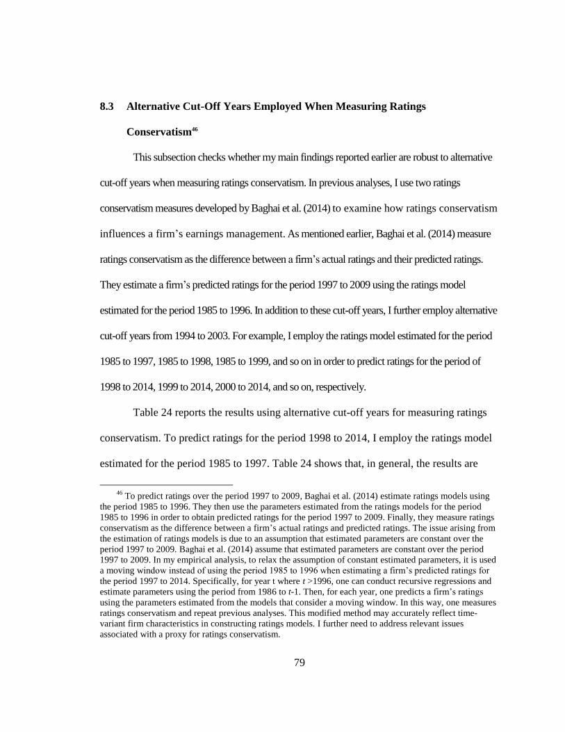
79

8.3 Alternative Cut-Off Years Employed When Measuring Ratings

Conservatism46

This subsection checks whether my main findings reported earlier are robust to alternative

cut-off years when measuring ratings conservatism. In previous analyses, I use two ratings

conservatism measures developed by Baghai et al. (2014) to examine how ratings conservatism

influences a firm’s earnings management. As mentioned earlier, Baghai et al. (2014) measure

ratings conservatism as the difference between a firm’s actual ratings and their predicted ratings.

They estimate a firm’s predicted ratings for the period 1997 to 2009 using the ratings model

estimated for the period 1985 to 1996. In addition to these cut-off years, I further employ alternative

cut-off years from 1994 to 2003. For example, I employ the ratings model estimated for the period

1985 to 1997, 1985 to 1998, 1985 to 1999, and so on in order to predict ratings for the period of

1998 to 2014, 1999 to 2014, 2000 to 2014, and so on, respectively.

Table 24 reports the results using alternative cut-off years for measuring ratings

conservatism. To predict ratings for the period 1998 to 2014, I employ the ratings model

estimated for the period 1985 to 1997. Table 24 shows that, in general, the results are

46

To predict ratings over the period 1997 to 2009, Baghai et al. (2014) estimate ratings models using

the period 1985 to 1996. They then use the parameters estimated from the ratings models for the period

1985 to 1996 in order to obtain predicted ratings for the period 1997 to 2009. Finally, they measure ratings

conservatism as the difference between a firm’s actual ratings and predicted ratings. The issue arising from

the estimation of ratings models is due to an assumption that estimated parameters are constant over the

period 1997 to 2009. Baghai et al. (2014) assume that estimated parameters are constant over the period

1997 to 2009. In my empirical analysis, to relax the assumption of constant estimated parameters, it is used

a moving window instead of using the period 1985 to 1996 when estimating a firm’s predicted ratings for

the period 1997 to 2014. Specifically, for year t where t >1996, one can conduct recursive regressions and

estimate parameters using the period from 1986 to t-1. Then, for each year, one predicts a firm’s ratings

using the parameters estimated from the models that consider a moving window. In this way, one measures

ratings conservatism and repeat previous analyses. This modified method may accurately reflect time-

variant firm characteristics in constructing ratings models. I further need to address relevant issues

associated with a proxy for ratings conservatism.

80

qualitatively similar to those reported in Tables 6 through 11. Specifically, with respect to

accrual-based earnings management measured as ABS_DA, the coefficient on

Lagged_Rat_Diff_Firm (Lagged_Rat_Diff_Ind) is negative and significant before (after)

controlling for REM1 and REM2, respectively. In contrast, the coefficient on REM1

(REM2) is positive and significant both before and after controlling for ABS_DA. Further,

the relation between ABS_DA and REM1 (REM2) is negative and significant. These

findings confirm my first hypothesis that ratings conservatism leads to less accrual-based

earnings management, but greater real earnings management.


Table 25 presents the results using alternative cut-off years for measuring ratings

conservatism. To do so, I employ the ratings model estimated for the period 1985 to 1998

in order to predict ratings for the period 1999 to 2014. The findings are qualitatively

similar to those reported in the main tables.


Overall, my main findings presented in Tables 6 through 11 are robust to alternative cut-off

years employed when I measure ratings conservatism.47

8.4 Controlling for the Effect of the Global Financial Crisis of 2007-2008

It is a possibility that external events such as the Global Financial Crisis of 2007 to 2008

bias estimates on the relation between ratings conservatism and earnings management. To address

47

In addition to these cut-off years, I also repeat analyses using alternative cut-off years from 1999 to

2002. The results, not reported for the sake of brevity, are qualitatively similar to my main findings.

81

this possibility, I re-estimate the regression equation (8) by controlling for an indicator variable for

the Global Financial Crisis of 2007-2008. The indicator variable takes the value of one if the years

are 2007 and 2008, and zero otherwise. Table 24 reports the results of pooled OLS regression that

control for the effect of external events, i.e., the Global Financial Crisis of 2007-2008. The results

are qualitatively similar to those reported in Tables 6 through 11. Thus, my main findings are robust

to the effect of external events.


Furthermore, I repeat the analysis in equation (8) after excluding sample periods of 2007-

2008 to mitigate the effect of the Global Financial Crisis on the relation between ratings

conservatism and earnings management. The unreported results, for the sake of brevity, are

qualitatively similar to those reported in Tables 6 through 11.

8.5 Possibility of Omitted Variable Bias

In this subsection, I check whether my main findings reported in Tables 6 through 11 are

robust to omitted variable bias. To mitigate the possibility of omitted variable problems, I re-

estimate the regression equation (8) after controlling for operating cycle (Cycle), cash flow

operations (CFO), sales growth (Sales_Growth), and a litigation indicator (LIT) as well as existing

control variables employed in equation.48 Based on prior studies on earnings management, I include

48

In addition to these additional variables, I plan on conducting analyses after controlling for corporate

governance characteristics (e.g., board size, board independence, board interlocks, CEO/Chair duality,

audit committee, foreign institutional ownership, and managerial ownership) that affect a firm’s earnings

management. The monitoring effectiveness of board of directors and audit committee on managerial

actions has been well explored in the accounting and finance literature. Generally, the board of directors is

recognized as entities that have the source and ability to effectively monitor managerial decisions (Jensen,

82

these control variables in equation (8). Specifically, following Cohen et al. (2008) and Zang (2012),

I control for operating cycles (Cycle).49 I measure Sales_Growth as the percentage of annual growth

in total sales. A litigation indicator (LIT) is defined in Appendix B.

Table 25 reports the results when I include additional control variables in equation (8). In

general, the results are qualitatively similar to those reported in Tables 6 through 11.


8.6 Re-estimation of the Regression Equation (8)

In this subsection, similar to Baghai et al. (2014), I re-estimate the regression equation (8)

using lagged explanatory variables, except for each ratings conservatism proxy lagged by two years,

as a robustness check. The lagged variables with two years can mitigate endogeneity problems. The

regression model is as follows:

1993; John and Senbet, 1998; Coles et al., 2013). For example, the key functions of board of directors are

to monitor and advise (top) management (Coles et al., 2013). Jensen (1993) and John and Senbet (1998)

emphasize the role of board of directors in monitoring management and their actions. They argue that the

effectiveness of monitoring is determined by composition of board of directors, board independence, and

board size. Given the above, in addition to audit committee, the board of directors is an effective monitor of

managers on behalf of shareholders because they are more likely to demand higher standards of corporate

governance (Gillan and Starks, 2003). Furthermore, following Zang (2012), I plan on conducting analyses

by controlling for the percentage of institutional ownership, firms’ marginal tax rates, and market shares.

For example, prior literature (Bushee, 1998; Roychowdhury, 2006; Zang, 2012) shows that institutional

ownership is effective in constraining real earnings management. 49

As in Cohen et al. (2008), the operating cycle is calculated as (𝐴𝑅t+𝐴𝑅t−1)/2

(𝑆𝐴𝐿𝐸𝑆

360)

+(𝐼𝑁𝑉𝑇t+𝐼𝑁𝑉𝑇t−1)/2

(𝐶𝑂𝐺𝑆

360)

. AR is

account receivable; SALES represents sales; INVT represents inventories; and COGS represents cost of

goods sold.

83

REMit (or AEMit) = β0 + β1Ratings_Conservatismit-2 + β2Sizeit-1 + β3Leverageit-1

+ β4MTBit-1 + β5ROAit-1 + β6Firm_Ageit-1 + β7Big4it-1 + β8SOXit-1

+ β9Z_Scoreit-1 + β10Lossit-1 + β11NOAit-1 + β12M&Ait-1 + β13Restructit-1

+ β14AEMit-1 (or REMit-1) + Σ βjIndustryj + Σ βkYeark + ɛit, (22)

where all variables are defined previously. I further include year and industry dummies (based on a

two-digit SIC industry) to control for time and industry specific effects. In addition, I use robust

standard errors clustered at the firm level. Untabulated results show that ratings conservatism

increases real earnings management, while decrease accrual-based earnings management, which

supports my first hypothesis (H1).

8.7 Validity of the Ratings Model50

For the robustness of the ratings model described in equation (1), I consider additional

specifications provided by Baghai et al. (2014). First, as in Baghai et al. (2014), I re-estimate the

ratings model by using only variables employed in Blume et al. (1998). Specifically, Blume et al.

(1998) employ the following variables in estimating the ratings model: (i) the operating margin,

calculated as the ratio of operating income before depreciation to sales; (ii) the ratio of long-term

debt to total assets; (iii) the ratio of total debt to total assets; (iv) the market value of equity; (v) a

firm’s beta from a market-model regression; (vi) the standard error from the market-model

regression; and (vii) a firm’s pretax interest coverage, computed as the ratio of sum of operating

50

I estimate several additional specifications of the ratings model and then repeat analyses using two

ratings conservatism proxies based on these specifications of the ratings model.

84

income after depreciation and interest expenses to interest expenses.51 Second, I re-estimate the

ratings model after including the square and cube terms of all explanatory variables to consider the

possibility of nonlinearities of the ratings model. Third, I repeat the ratings model by considering

firm size and leverage in terms of market values, not book values. Specifically, I employ book

leverage (calculated as the ratio of total debt to book value of assets) and firm size (computed as the

logarithm of book value of assets) in equation (1). Instead, I replace these variables expressed in

book values with them expressed in market values. Finally, I estimate the ratings model by

considering serval macroeconomic variables. These macroeconomic variables includes the

following: (i) the inflation rates; (ii) the rates of GDP growth; (iii) the slope of term structure52; (iv)

the TED spread53; (v) the ratio of price to earnings; and (vi) the market volatility index. Untabulated

results indicate that our main findings are robust these different specifications for ratings model.

8.8 Role of Accounting Quality in the Assignment of Credit Ratings

In this subsection, I consider the role of accounting quality in the assignment of credit

ratings. As mentioned previously, credit rating agencies consider accounting quality in assigning

credit ratings (Ashbaugh-Skaife et al., 2006; Jorion et al., 2009; Caton et al., 2011; Bae et al., 2013;

Shen and Huang, 2013; Standard & Poor’s, 2015). Ashbaugh-Skaife et al., (2006) provide evidence

that credit ratings are positively related to accounting quality, indicating that accounting quality is

51

See Blume et al. (1998, p. 1394-1395) for more details on these variables. 52

The slope of term structure is computed as the difference between the constant-maturity 10-year

Treasury bond yield and the constant-maturity three-month T-bill yield. 53

The TED spread is calculated as the three-month London Interbank Offered Rate (LIBOR) minus the

three-month T-bill rate.

85

considered as one of the important components in rating assignment by ratings agencies.54 In a

subsequent study, Jorion et al. (2009) emphasize the importance of accounting quality in the

downward trend in credit ratings over time. They argue that a decline in accounting quality can

primarily explain the downward trend in credit ratings. In a more recent study, Bae et al. (2013)

argue that after the assignment of initial credit ratings by S&P, firms tend to engage in less accrual-

based earnings management.

Thus, I re-estimate the rating model (1) after including accounting quality proxies (e.g.,

discretionary accruals) and predict ratings. I then calculate ratings conservatism as the difference

between a firm’s actual ratings and predicted ratings. Finally, I repeat the analysis using the ratings

conservatism proxies to check the robustness of the main results reported in Tables 6 through 15.

54

In contrast, the following studies argue that credit ratings agencies cannot fully understand the

process of a firm’s accounting accruals and thus managers manage earnings to favorably influence their

debt ratings. For example, Gu and Zhao (2006) find evidence of a positive relation between accrual-based

earnings management and bond ratings. This finding suggests that firms are likely to receive better debt

ratings when they engage in more earnings management. They further show that the downward trend in

bond ratings may not be due to accrual-based earnings management. Similarly, Demirtas and Cornaggia

(2013) find that there are high current accruals at the time of initial credit ratings. This finding indicates

that firms manage earnings around initial credit ratings in an attempt to obtain better initial ratings.

86

CHAPTER 9

CONCLUSION

The objective of this study is to examine whether ratings conservatism by credit ratings

agencies can affect a firm’s earnings management. I predict that managers take different earnings

management strategies in response to the tightening of credit standards by rating agencies.

Specifically, I investigate whether ratings conservatism leads to a substitution between an increase

in real earnings management and a decrease in accrual-based earnings management. To this end, I

test the following hypotheses and predictions. First, I hypothesize that tighter rating standards by

credit rating agencies lead to a substitution between real and accrual-based earnings management.

Consistent with the first hypothesis, I find that ratings conservatism is associated with lower

accrual-based earnings management, measured through the absolute value of discretionary accruals

and positive and negative discretionary accruals. In contrast, I find that these firms engage in more

real earnings management, measured as the abnormal levels of production costs, discretionary

expenses, and cash flow from operations as well as aggregate measures of real earnings

management. Further, I find that total earnings management, calculated as the signed discretionary

accruals and each aggregate measure of real earnings management, increases in response to ratings

conservatism. This finding indicates that the increase in real earnings management is greater than

the decrease in accrual-based earnings management. Second, I hypothesize that a positive

(negative) relation between ratings conservatism and real earnings management (accrual-based

earnings management) is more pronounced for firms with low credit quality than for those with

high credit quality. I find that the negative relation between ratings conservatism and

87

accrual-based earnings management, measured as the absolute value of discretionary

accruals, is stronger for speculative-grade firms than for investment-grade firms.

However, I find that the positive relation between ratings conservatism and real earnings

management does not apply to both investment- and speculative-grade firms. Finally, I test whether

ratings conservatism is associated with other types of earnings management, such as income

smoothing and asymmetric timeliness loss recognition. With respect to the additional analyses, I

find no evidence that firms affected more by ratings conservatism tend to engage in more or even

less earnings smoothing. I also find inconsistent results regarding the relation between ratings

conservatism and each measure of asymmetric timeliness loss recognition. Overall, this study

shows that ratings conservatism affects a firm’s incentive to manage its reported

earnings. More importantly, this study suggests that ratings conservatism can influence a

firm’s choice between accrual-based and real earnings management.

88

CHAPTER 10

LIMITATIONS AND FUTURE RESEARCH

Although my study provides useful information to the literature, there are some limitations

and future directions that will be addressed. First, it is unclear whether Standard & Poor’s (S&P) is

generally becoming more conservative over time for all firms or S&P is more conservative for

certain types of firms. This distinction is needed for the story of how the empirics work. If it is the

former instead of the later, then estimating discretionary accruals by each year does not seem

correct. It would be helpful to show that there is cross-sectional variation in ratings conservatism

each year if discretionary accruals are estimated by year. Second, regarding accrual-based earnings

management, it would be interesting to test the following research questions: Do firms that respond

with less accrual-based earnings management have a lower level of debt? Are the firms with less

accrual-based earnings management more likely to borrow? Does this type of earnings

management strategy work? If so, do firms experience improvement in credit ratings after they

engage in less accrual-based earnings management? Third, for an additional cross-sectional test that

could be interesting, future research may need to split the sample by firms that want to borrow. This

would be consistent with the story if the effect is stronger for firms that borrow in the subsequent

year. Further, there is a possibility of reverse causality. For example, firms are more likely to borrow

when their credit rating improves, but it still could add to the paper. Fourth, it would help if future

research discusses some more details or provides certain anecdotal evidence on how credit rating

agencies analyze firms’ earnings quality. Finally, it would be more interesting if future research

includes additional cross-sectional tests. For instance, would the effect of ratings conservatism vary

89

among firms with different institutional ownership or analyst coverage? Prior literature shows that

institutional ownership and financial analysts act as firms’ external monitors. Thus, I would expect

the relation between ratings conservatism and accrual-based earnings management to be more

pronounced in firms with less institutional ownership or analyst coverage.

90

APPENDIX A

VARIABLE DEFINITIONS: RATINGS MODEL55

Variable Name Description

Book_Lev The sum of long- and short-term debt divided by total assets;

Conb The ratio of convertible debt to total assets;

Rentp The ratio of rental payments to total assets;

Cash The sum of cash and marketable securities divided by total assets;

Debt_Ebitda The ratio of total debt to earnings before interest, taxes,

depreciation and amortization (EBITDA);

Net_Debt_Ebitda A dummy variable equal to one if the ratio of total debt to EBITDA

is negative, and zero otherwise;

Ebitda_Int The EBITDA divided by interest payments;

Profit The ratio of EBITDA to sales;

Vol_Profit The volatility of Profit;

Firm_Size The logarithm of book value of assets;

Tangibility The ratio of net property, plant, and equipment (NPPE) divided by

total assets;

Capex Capital expenditures divided by total assets;

Beta The stock’s Dimson beta, estimated from a market-model

regression using the daily CRSP value-weighted index returns;

Idiosyncratic_Risk The root-mean-squared error (RMSE) from a market-model

regression.

55

I estimate the ratings model using variables employed in Baghai et al. (2014).

91

APPENDIX B

VARIABLE DEFINITIONS: BASELINE REGRESSION MODEL

Variables Description

Panel A: Accrual-Based Earnings Management (AEM)

TA The difference between income before extraordinary items

(Compustat Data Item #123) and operating cash flows (Compustat

Data Item #308);

AT Total assets (Compustat Data Item #6);

ΔREV The change in net sales (Compustat Data Item #12) from the previous

year;

ΔAR The change in accounts receivable (Compustat Data Item #2) from

the previous year;

PPE The gross property, plant, and equipment (Compustat Data Item #7);

DA The discretionary accruals calculated using the Modified Jones

Model;

ABS_DA The absolute value of the discretionary accruals calculated using the

Modified Jones model;

Positive_DA The positive value of discretionary accruals calculating using the

Modified Jones model;

Negative_DA The negative value of discretionary accruals calculating using the

Modified Jones model.

Panel B: Real Earnings Management (REM)

CFO The cash flow from operations (Compustat Data Item #308 minus

Compustat Data Item #124);

ΔSALE The change in net sales (Compustat Data Item #12) from the previous

year;

COGS The cost of goods sold (Compustat Data Item #41);

92

ΔINVT The change in inventories (Compustat Data Item #3);

PROD The production costs, calculated as the sum of COGS and ΔINVT;

DISX The discretionary expenditures, calculated as the sum of R&D

expenses (Compustat Data Item #46), SG&A (Compustat Data Item

#189), and advertising expenses (Compustat Data Item #45), where

as long as SG&A is available, R&D and advertising expenses are set

to zero if they are missing;

REM_CFO The abnormal cash flow from operations (measured as the difference

between the actual CFO and the fitted normal levels of CFO),

multiplied by negative one;

REM_PROD The abnormal levels of production costs (PROD), measured as the

difference between the actual PROD and the fitted normal levels of

PROD;

REM_DISX The abnormal levels of discretionary expenses (measured as the

difference between the actual DISX and the fitted normal levels of

DISX), multiplied by negative one;

REM1 The aggregate measure of real earnings management, computed as

REM_DISX + REM_PROD;

REM2 The aggregate measure of real earnings management, calculated as

REM_DISX + REM_CFO.

Panel C: Total Earnings Management (TEM)

TEM1 The sum of the signed discretionary accruals (DA) and the aggregate

real earnings management (REM1);

TEM2 The sum of the signed discretionary accruals (ABS_DA) and the

aggregate real earnings management (REM2).

Panel D: Earnings Smoothing

σ(Earnings)/σ(CFO) The ratio of standard deviation of earnings to standard deviation of

cash flow from operations (CFO), both scaled by lagged total assets;

93

ρ(∆ACC, ∆CFO) The Spearman correlation between the change in total accruals (ACC)

and the change in cash flow from operations, both scaled by lagged

total assets;

ρ(∆DA, ∆PDI) The Spearman correlation between the change in discretionary

accruals and the change in pre-discretionary income, where DA refers

to discretionary accruals and PDI is the pre-discretionary income

(‘un-managed income’), calculated as net income before

extraordinary income minus discretionary accruals, i.e., PDI = NI –

DAP;

EM_SMOOTH1 Earnings smoothing ranking of σ(Earnings)/σ(CFO). Following

Zarowin (2002), I convert σ(Earnings)/σ(CFO) into reverse fractional

ranking by each two-digit SIC industry and year. A higher rank

indicates more earnings smoothing;

EM_SMOOTH2 Earnings smoothing ranking of ρ(∆ACC, ∆CFO). Following Tucker

and Zarowin (2006), I convert the correlation into reverse fractional


indicates more earnings smoothing;

EM_SMOOTH3 Earnings smoothing ranking of ρ(∆DA, ∆PDI). I follow Tucker and

Zarowin (2006) and convert the correlation into reverse fractional


indicates more earnings smoothing.

Panel D: Explanatory Variables (Equations 8 and 13)

Rat_Diff_Firm The difference between a firm’s actual and predicted ratings, where

the predicted ratings are estimated based on firm fixed effects (from

model (6) of Table 3);

Rat_Diff_Ind The difference between a firm’s actual and predicted ratings, where

the predicted ratings are estimated based on industry fixed effects

(from model (3) of Table 3);

94

Size56 The natural logarithm of the market value of total assets, where the

market value of total assets is calculated as the market value of equity

plus the book value of total assets minus the book value of total

equity;

Leverage57 The ratio of long-term debt to the market value of total assets;

MTB The ratio of the market value of equity to the book value of equity;

ROA The earnings before interest, taxes, depreciation, and amortization

(EBITDA) divided by lagged total assets;

Firm_Age An indicator variable equal to one if a firm listed on Compustat has

more than 20 years, and zero otherwise;

Big4 An indicator variable equal to one if a firm’s auditor is one of the

Big 4 audit firms, and zero otherwise;

SOX An indicator variable equal to one if the year is 2002 or later, and

zero otherwise;

Z_Score The modified version of Altman’s Z-score, calculated as Z = 0.3(net

income/total assets) + 1.0(sales/total assets) + 1.4(retained

earnings/total assets) + 0.6(market value of equity/total liabilities);

Loss An indicator variable equal to one if net income is less than zero, and

zero otherwise;

NOA An indicator variable equal to one if the net operating assets at the

beginning of the year divided by lagged sales above the median of the

corresponding industry-year, and zero otherwise;

M&A An indicator variable equal to one if the auditee is engaged in a

merger or acquisition, and zero otherwise;

Restruct An indicator variable equal to one if the firm took restricting charges,

and zero otherwise.

56

Results are qualitatively similar to those reported in Tables 6 through 15 if I define Size as the

natural logarithm of total assets. 57

Results are qualitatively similar to those reported in Tables 6 through 15 if I define Leverage as

long- and short-term debt divided by book value of total assets.

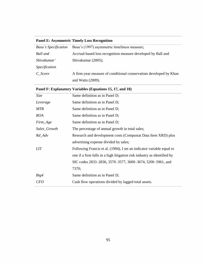
95

Panel E: Asymmetric Timely Loss Recognition

Basu’s Specification Basu’s (1997) asymmetric timeliness measure;

Ball and

Shivakumar’

Specification

Accrual-based loss recognition measure developed by Ball and

Shivakumar (2005);

C_Score A firm-year measure of conditional conservatism developed by Khan

and Watts (2009).

Panel F: Explanatory Variables (Equations 15, 17, and 18)

Size Same definition as in Panel D;

Leverage Same definition as in Panel D;

MTB Same definition as in Panel D;

ROA Same definition as in Panel D;

Firm_Age Same definition as in Panel D;

Sales_Growth The percentage of annual growth in total sales;

Rd_Adv Research and development costs (Compustat Data Item XRD) plus

advertising expense divided by sales;

LIT Following Francis et al. (1994), I set an indicator variable equal to

one if a firm falls in a high litigation risk industry as identified by

SIC codes 2833–2836, 3570–3577, 3600–3674, 5200–5961, and

7370;

Big4 Same definition as in Panel D;

CFO Cash flow operations divided by lagged total assets.

96

APPENDIX C

MEASURE OF ASYMMETRIC TIMELY LOSS RECOGNITION: Khan and

Watts’ C_Score (2009, p. 136)

Based on the Basu’s (1997) measure of asymmetric timeliness, Khan and Watts

(2009) develop a firm-specific measure of the asymmetric timeliness. Khan and Watts

(2009) estimate the timelines of good news (G_Score) and bad news (C_Score) as

follows:

NIi = β1 + β2Di + β3RETi + β4 Di * RETi +ɛi (a)

G_Score = β3 = μ1 + μ2SIZEi + μ3MTBi + μ4LEVi +ɛi (b)

C_Score = β4 = λ1 + λ2SIZEi + λ3MTBi + λ4LEVi +ɛi, (c)

where the subscript i indicates the firm, NI is annual earnings, RET is returns, D is an

indicator variable equal to one when RET<0 and zero otherwise. SIZE is the logarithm of

the market value of equity. MTB is the ratio of market value of equity to book value of

equity. LEV is the total debt divided by market value of equity. Replacing β3 and β4

estimated from equations (b) and (c) into regression equation (a) and including additional

terms in the last parenthesis yields the following equation:

Xi = β1 + β2Di + RETi * (μ1 + μ2SIZEi + μ3MTBi + μ4LEVi)

+ Di * RETi *(λ1 + λ2SIZEi + λ3MTBi + λ4LEVi)

+ (δ1SIZEi + δ2MTBi + δ3LEVi + δ4Di * SIZEi + δ5Di * MTBi + δ6Di * LEVi) + ɛi (d)

I estimate the above equation (d) using annual cross-sectional regressions. Then, I

obtain G_Score and C_Score using the coefficients estimated from equation (d). In the

analysis, I use C_Score for capturing a firm’s asymmetric timely loss recognition (also

for measuring a firm’s conditional accounting conservatism). All variables used are


97

Table 1 Number of Firms by S&P Credit Ratings Categories and Year, 1985-2014

(CHAPTER 4)

This table shows the distribution of credit ratings over the period 1985 to 2014. My sample contains 35,160

firm-year observations of ratings. For the convenience, I combine minus (−), middle, and plus (+)

specifications for each broad credit rating. For example, the AA category includes credit ratings of AA+,

AA, and AA−.

Rating

Year AAA AA A BBB BB B CCC CC C Total

1985 28 103 197 118 131 160 6 1 0 744

1986 28 108 194 144 173 246 48 0 0 941

1987 31 108 185 133 170 255 33 2 0 917

1988 34 87 201 139 156 263 29 0 0 909

1989 35 87 189 151 153 234 31 0 1 881

1990 33 86 193 151 150 188 36 0 3 840

1991 32 87 196 165 159 159 34 9 0 841

1992 30 85 198 188 189 156 23 6 0 875

1993 28 84 198 208 229 178 12 1 0 938

1994 26 79 202 221 237 194 14 1 0 974

1995 27 77 216 243 263 224 17 0 0 1,067

1996 25 82 228 285 288 259 17 2 0 1,186

1997 24 81 235 319 340 319 11 2 0 1,331

1998 21 80 230 349 368 344 23 6 0 1,421

1999 17 68 218 370 372 349 30 10 0 1,434

2000 14 49 232 381 361 384 43 7 0 1,471

2001 13 47 217 388 365 363 55 13 0 1,461

2002 11 41 209 379 385 328 71 14 0 1,438

2003 11 38 202 373 418 374 61 5 0 1,482

2004 9 37 197 376 423 365 44 4 0 1,455

2005 9 34 194 351 397 359 46 2 0 1,392

2006 9 34 167 335 391 378 33 2 0 1,349

2007 7 33 156 328 357 352 22 4 0 1,259

2008 6 32 149 313 316 327 53 12 0 1,208

2009 5 32 146 323 297 345 39 2 0 1,189

2010 6 30 145 337 313 351 23 5 0 1,210

2011 6 27 144 341 323 336 24 1 0 1,202

2012 6 28 143 348 324 354 22 1 0 1,226

2013 6 33 142 355 350 336 27 0 0 1,249

2014 5 35 138 353 368 347 24 0 0 1,270

Total 542 1832 5661 8465 8766 8827 951 112 4 35,160

98

Table 2 Summary Statistics for Relevant Variables used in Ratings Models (CHAPTER 4)

This table reports descriptive statistics for variables used in the ratings model (1). This table shows that the average ratings variable (Rating) has

increased from 8.876 in 1985 to 11.150 in 2014. All variables are defined in Appendix A.

Year Rating Book_Lev Conb Rentp Cash Debt_Ebitda Net_Debt_Ebitda Ebitda_Int Profit Vol_Profit Firm_Size Tangibility Capex

1985 8.876 0.326 0.042 0.024 0.079 2.962 0.034 7.868 0.159 0.036 6.840 0.451 0.088

1986 9.944 0.363 0.051 0.025 0.090 3.511 0.052 7.344 0.143 0.058 6.651 0.416 0.076

1987 9.913 0.377 0.055 0.025 0.088 3.352 0.046 6.996 0.161 0.051 6.801 0.408 0.073

1988 9.878 0.392 0.046 0.025 0.077 3.457 0.035 7.334 0.166 0.049 6.967 0.406 0.074

1989 9.796 0.405 0.038 0.024 0.069 3.508 0.035 6.248 0.164 0.120 7.106 0.416 0.075

1990 9.638 0.403 0.033 0.024 0.065 3.400 0.032 6.741 0.161 0.106 7.226 0.424 0.074

1991 9.529 0.393 0.033 0.026 0.065 3.765 0.027 6.614 0.158 0.039 7.281 0.433 0.068

1992 9.477 0.382 0.035 0.026 0.066 3.540 0.025 8.334 0.157 0.037 7.298 0.433 0.069

1993 9.549 0.375 0.034 0.026 0.071 3.519 0.031 7.956 0.143 0.042 7.300 0.429 0.072

1994 9.715 0.375 0.032 0.025 0.065 3.287 0.031 8.916 0.154 0.051 7.329 0.425 0.074

1995 9.845 0.382 0.029 0.024 0.066 3.204 0.032 8.931 0.157 0.058 7.341 0.410 0.078

1996 10.006 0.386 0.027 0.024 0.068 3.318 0.037 8.803 0.139 0.162 7.359 0.410 0.079

1997 10.243 0.400 0.027 0.024 0.075 3.398 0.042 10.216 0.109 0.268 7.332 0.399 0.082

1998 10.443 0.442 0.023 0.026 0.068 3.839 0.055 9.504 0.065 0.357 7.393 0.388 0.082

1999 10.628 0.440 0.020 0.024 0.072 3.764 0.059 7.987 0.096 0.378 7.485 0.375 0.071

2000 10.821 0.427 0.021 0.024 0.072 3.491 0.068 8.203 0.123 0.405 7.551 0.365 0.070

2001 10.934 0.424 0.023 0.026 0.078 3.853 0.057 8.161 0.150 0.094 7.561 0.364 0.064

2002 11.043 0.415 0.024 0.026 0.084 3.679 0.040 10.323 0.142 0.085 7.602 0.361 0.052

2003 11.142 0.398 0.025 0.025 0.093 3.815 0.026 11.782 0.096 0.285 7.689 0.351 0.049

2004 11.073 0.375 0.024 0.023 0.097 3.188 0.014 16.014 0.154 0.297 7.791 0.339 0.052

2005 11.114 0.358 0.021 0.022 0.097 3.086 0.014 18.579 0.174 0.313 7.863 0.325 0.057

2006 11.211 0.356 0.021 0.021 0.090 3.025 0.015 18.016 0.170 0.188 7.953 0.325 0.063

2007 11.155 0.364 0.019 0.020 0.085 3.155 0.022 15.384 0.164 0.194 8.082 0.325 0.064

2008 11.380 0.386 0.019 0.022 0.087 3.281 0.050 14.338 0.154 0.212 8.109 0.337 0.065

2009 11.297 0.366 0.017 0.022 0.109 3.494 0.044 13.524 0.163 0.147 8.123 0.337 0.048

2010 11.203 0.351 0.016 0.020 0.108 3.127 0.016 17.561 0.202 0.148 8.184 0.332 0.051

2011 11.113 0.359 0.012 0.019 0.099 3.040 0.017 16.198 0.206 0.157 8.232 0.329 0.058

2012 11.140 0.366 0.010 0.018 0.098 3.420 0.016 17.685 0.167 0.165 8.289 0.330 0.064

2013 11.151 0.369 0.008 0.018 0.102 3.435 0.024 16.134 0.202 0.067 8.300 0.336 0.061

2014 11.150 0.382 0.008 0.018 0.099 3.594 0.020 16.260 0.195 0.064 8.321 0.332 0.062

Mean 10.593 0.386 0.025 0.023 0.084 3.426 0.034 11.670 0.151 0.170 7.617 0.371 0.066

N 35,160 34,993 34,601 30,548 35,055 34,642 35,160 34,641 35,009 35,160 33,354 34,877 34,552

99

Table 3 Ratings Models (CHAPTER 4)

This table shows the results of the ratings model on the relation between each explanatory variable and credit ratings. In columns (1), (3), (5), and (6), I

run pooled OLS regressions. I also run ordered logit regressions in columns (2) and (4). In the first four columns, I consider industry and year fixed

effects. Furthermore, I consider firm and year fixed effects in the last two models. The results reported in all columns (1) through (6) are consistent with

Baghai et al. (2014). All variables are defined in Appendix A.

(1) (2) (3) (4) (5) (6)

Rating Coef. P-value Coef. P-value Coef. P-value Coef. P-value Coef. P-value Coef. P-value

Book_Lev 2.986 0.000 2.665 0.000 2.609 0.000 2.576 0.000 2.616 0.000 2.575 0.000

Conb 2.575 0.000 1.599 0.000 2.402 0.000 2.049 0.000 0.659 0.099 0.526 0.169

Rentp 4.021 0.001 4.654 0.000 4.104 0.002 5.064 0.000 2.190 0.239 3.985 0.060

Cash 0.589 0.071 0.678 0.011 0.105 0.735 0.343 0.223 -0.437 0.151 -0.208 0.518

Debt_Ebitda 0.262 0.000 0.263 0.000 0.179 0.000 0.199 0.000 0.114 0.000 0.088 0.000

Net_Debt_Ebitda 3.329 0.000 3.491 0.000 1.960 0.000 2.545 0.000 1.590 0.000 1.173 0.000

Ebitda_Int -0.005 0.000 -0.004 0.001 -0.005 0.000 -0.005 0.001 -0.002 0.000 -0.002 0.000

Profit -0.091 0.001 -0.091 0.002 -0.064 0.005 -0.075 0.004 -0.009 0.673 -0.011 0.435

Vol_Profit 0.012 0.034 0.019 0.014 0.002 0.741 0.009 0.324 0.006 0.442 0.003 0.705

Firm_Size -1.275 0.000 -1.061 0.000 -1.103 0.000 -0.995 0.000 -1.073 0.000 -1.037 0.000

Tangibility -1.130 0.000 -0.616 0.008 0.292 0.263 0.389 0.096 -1.043 0.006 -1.350 0.002

Capex -1.517 0.020 -1.673 0.002 -2.440 0.000 -2.535 0.000 -4.953 0.000 -4.290 0.000

Beta - - - - 0.251 0.000 0.187 0.000 - - 0.079 0.000

Idiosyncratic_Risk - - - - 2.032 0.000 2.417 0.000 - - 1.188 0.000

1986 0.372 0.000 0.247 0.000 0.309 0.002 0.244 0.005 0.310 0.000 0.354 0.000

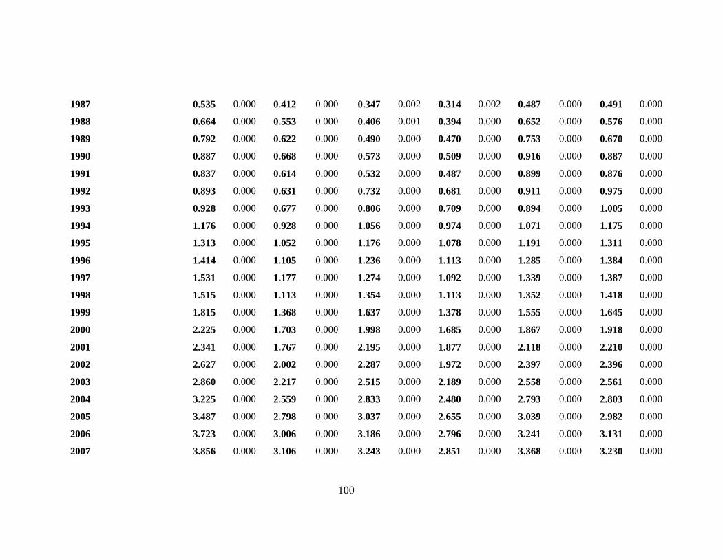
100

1987 0.535 0.000 0.412 0.000 0.347 0.002 0.314 0.002 0.487 0.000 0.491 0.000

1988 0.664 0.000 0.553 0.000 0.406 0.001 0.394 0.000 0.652 0.000 0.576 0.000

1989 0.792 0.000 0.622 0.000 0.490 0.000 0.470 0.000 0.753 0.000 0.670 0.000

1990 0.887 0.000 0.668 0.000 0.573 0.000 0.509 0.000 0.916 0.000 0.887 0.000

1991 0.837 0.000 0.614 0.000 0.532 0.000 0.487 0.000 0.899 0.000 0.876 0.000

1992 0.893 0.000 0.631 0.000 0.732 0.000 0.681 0.000 0.911 0.000 0.975 0.000

1993 0.928 0.000 0.677 0.000 0.806 0.000 0.709 0.000 0.894 0.000 1.005 0.000

1994 1.176 0.000 0.928 0.000 1.056 0.000 0.974 0.000 1.071 0.000 1.175 0.000

1995 1.313 0.000 1.052 0.000 1.176 0.000 1.078 0.000 1.191 0.000 1.311 0.000

1996 1.414 0.000 1.105 0.000 1.236 0.000 1.113 0.000 1.285 0.000 1.384 0.000

1997 1.531 0.000 1.177 0.000 1.274 0.000 1.092 0.000 1.339 0.000 1.387 0.000

1998 1.515 0.000 1.113 0.000 1.354 0.000 1.113 0.000 1.352 0.000 1.418 0.000

1999 1.815 0.000 1.368 0.000 1.637 0.000 1.378 0.000 1.555 0.000 1.645 0.000

2000 2.225 0.000 1.703 0.000 1.998 0.000 1.685 0.000 1.867 0.000 1.918 0.000

2001 2.341 0.000 1.767 0.000 2.195 0.000 1.877 0.000 2.118 0.000 2.210 0.000

2002 2.627 0.000 2.002 0.000 2.287 0.000 1.972 0.000 2.397 0.000 2.396 0.000

2003 2.860 0.000 2.217 0.000 2.515 0.000 2.189 0.000 2.558 0.000 2.561 0.000

2004 3.225 0.000 2.559 0.000 2.833 0.000 2.480 0.000 2.793 0.000 2.803 0.000

2005 3.487 0.000 2.798 0.000 3.037 0.000 2.655 0.000 3.039 0.000 2.982 0.000

2006 3.723 0.000 3.006 0.000 3.186 0.000 2.796 0.000 3.241 0.000 3.131 0.000

2007 3.856 0.000 3.106 0.000 3.243 0.000 2.851 0.000 3.368 0.000 3.230 0.000

101

2008 3.921 0.000 3.156 0.000 3.304 0.000 2.956 0.000 3.545 0.000 3.405 0.000

2009 3.849 0.000 3.122 0.000 3.240 0.000 2.917 0.000 3.453 0.000 3.315 0.000

2010 4.108 0.000 3.320 0.000 3.474 0.000 3.109 0.000 3.526 0.000 3.386 0.000

2011 4.068 0.000 3.274 0.000 3.439 0.000 3.050 0.000 3.523 0.000 3.365 0.000

2012 4.054 0.000 3.228 0.000 3.470 0.000 3.060 0.000 3.543 0.000 3.393 0.000

2013 4.009 0.000 3.201 0.000 3.487 0.000 3.073 0.000 3.514 0.000 3.352 0.000

2014 3.979 0.000 3.156 0.000 3.419 0.000 3.008 0.000 3.418 0.000 3.280 0.000

Industry dummies Y - Y - Y - Y - N - N -

Firm dummies N - N - N - N - Y - Y -

Observations 27,631 - 27,631 - 21,528 - 21,528 - 27,631 - 21,528 -

Adjusted R2 0.642 - - - 0.689 - - - 0.888 - 0.893 -

Pseudo R2 - - 0.206 - - - 0.243 - - - - -

102

Table 4 Descriptive Statistics (CHAPTER 5)

This table shows descriptive statistics for relevant variables used in the analysis. My sample period is

between 1997 and 2014. All variables are defined in Appendix B.

Variable N Mean Std. Dev. 25th Pctl. Median 75th Pctl.

DA 11,499 0.0017 0.0712 -0.0255 0.0060 0.0365

ABS_DA 11,499 0.0482 0.0550 0.0141 0.0315 0.0612

REM_PROD 11,499 0.0023 0.1422 -0.0719 0.0044 0.0833

REM_DISX 11,499 0.0079 0.1570 -0.0577 0.0174 0.0924

REM_CFO 11,499 -0.0015 0.0693 -0.0407 -0.0006 0.0371

REM1 11,499 0.0111 0.2652 -0.1187 0.0208 0.1691

REM2 11,499 0.0069 0.1702 -0.0754 0.0169 0.1071

TEM1 11,499 0.0595 0.2704 -0.0767 0.0663 0.2177

TEM2 11,499 0.0553 0.1788 -0.0378 0.0584 0.1585

EM_SMOOTH1 9,981 0.5113 0.2925 0.2632 0.5169 0.7636

EM_SMOOTH2 9,962 0.5021 0.2885 0.2553 0.5250 0.7732

EM_SMOOTH3 9,874 0.5141 0.2857 0.2727 0.5227 0.7619

Rat_Diff_Firm 11,499 0.4749 5.5444 -0.3494 2.1064 3.7663

Rat_Diff_Ind 11,499 0.6193 5.5226 0.1721 2.2817 3.8094

Size 11,499 8.4460 1.5098 7.3927 8.3188 9.4424

Leverage 11,499 0.2329 0.1706 0.1017 0.1956 0.3295

MTB 11,499 2.8671 5.3716 1.2540 2.1387 3.5486

ROA 11,499 0.0956 0.0989 0.0508 0.0943 0.1449

Firm_Age 11,499 0.4794 0.4996 0.0000 0.0000 1.0000

Big4 11,499 0.9080 0.2890 1.0000 1.0000 1.0000

SOX 11,499 0.7230 0.4475 0.0000 1.0000 1.0000

Z_Score 11,499 8.3083 39.6864 1.9198 3.3597 5.7348

Loss 11,499 0.2399 0.4271 0.0000 0.0000 0.0000

NOA 11,499 0.5306 0.4991 0.0000 1.0000 1.0000

M&A 11,499 0.1621 0.3686 0.0000 0.0000 0.0000

Restruct 11,499 0.3803 0.4855 0.0000 0.0000 1.0000

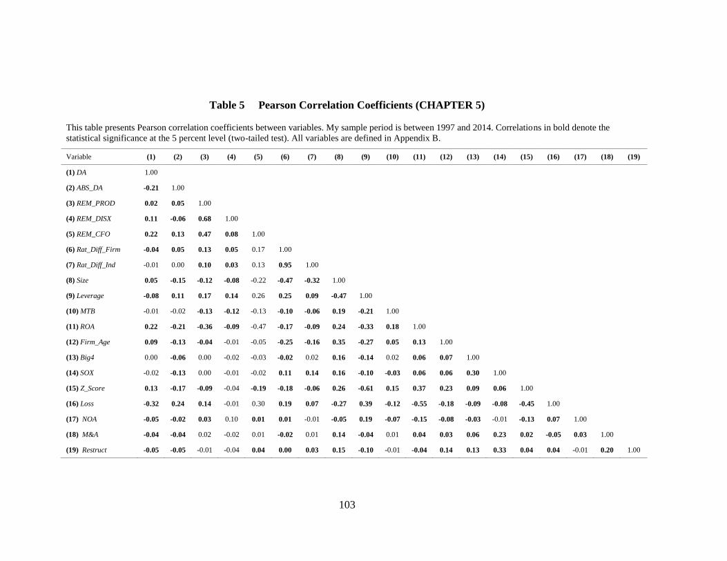
103

Table 5 Pearson Correlation Coefficients (CHAPTER 5)

This table presents Pearson correlation coefficients between variables. My sample period is between 1997 and 2014. Correlations in bold denote the

statistical significance at the 5 percent level (two-tailed test). All variables are defined in Appendix B.

Variable (1) (2) (3) (4) (5) (6) (7) (8) (9) (10) (11) (12) (13) (14) (15) (16) (17) (18) (19)

(1) DA 1.00

(2) ABS_DA -0.21 1.00

(3) REM_PROD 0.02 0.05 1.00

(4) REM_DISX 0.11 -0.06 0.68 1.00

(5) REM_CFO 0.22 0.13 0.47 0.08 1.00

(6) Rat_Diff_Firm -0.04 0.05 0.13 0.05 0.17 1.00

(7) Rat_Diff_Ind -0.01 0.00 0.10 0.03 0.13 0.95 1.00

(8) Size 0.05 -0.15 -0.12 -0.08 -0.22 -0.47 -0.32 1.00

(9) Leverage -0.08 0.11 0.17 0.14 0.26 0.25 0.09 -0.47 1.00

(10) MTB -0.01 -0.02 -0.13 -0.12 -0.13 -0.10 -0.06 0.19 -0.21 1.00

(11) ROA 0.22 -0.21 -0.36 -0.09 -0.47 -0.17 -0.09 0.24 -0.33 0.18 1.00

(12) Firm_Age 0.09 -0.13 -0.04 -0.01 -0.05 -0.25 -0.16 0.35 -0.27 0.05 0.13 1.00

(13) Big4 0.00 -0.06 0.00 -0.02 -0.03 -0.02 0.02 0.16 -0.14 0.02 0.06 0.07 1.00

(14) SOX -0.02 -0.13 0.00 -0.01 -0.02 0.11 0.14 0.16 -0.10 -0.03 0.06 0.06 0.30 1.00

(15) Z_Score 0.13 -0.17 -0.09 -0.04 -0.19 -0.18 -0.06 0.26 -0.61 0.15 0.37 0.23 0.09 0.06 1.00

(16) Loss -0.32 0.24 0.14 -0.01 0.30 0.19 0.07 -0.27 0.39 -0.12 -0.55 -0.18 -0.09 -0.08 -0.45 1.00

(17) NOA -0.05 -0.02 0.03 0.10 0.01 0.01 -0.01 -0.05 0.19 -0.07 -0.15 -0.08 -0.03 -0.01 -0.13 0.07 1.00

(18) M&A -0.04 -0.04 0.02 -0.02 0.01 -0.02 0.01 0.14 -0.04 0.01 0.04 0.03 0.06 0.23 0.02 -0.05 0.03 1.00

(19) Restruct -0.05 -0.05 -0.01 -0.04 0.04 0.00 0.03 0.15 -0.10 -0.01 -0.04 0.14 0.13 0.33 0.04 0.04 -0.01 0.20 1.00

104

Table 6 Relation between Ratings Conservatism and Accrual-Based Earnings Management


This table reports the results of pooled OLS regression with ABS_DA, Positive_DA, and Negative_DA as each dependent variable. The main variable of interest

is Lagged_Rat_Diff_Firm. I use a sample of 9,837, 5,548, and 4,289 firm-year observations for ABS_DA, Positive_DA, and Negative_DA, respectively, between

1997 and 2014. I use robust standard errors clustered at the firm level. All continuous variables are winsorized at the 1% and 99% level s. The p-values are in

parentheses. ***, **, and * denote the statistical significance at the 1 percent, 5 percent, and 10 percent levels, respectively (two-tailed test). All variables are


Dependent variables:

Explanatory variables ABS_DA

(1)

Positive_DA

(2)

Negative_DA

(3)

ABS_DA

(4)

Positive_DA

(5)

Negative_DA

(6)

ABS_DA

(7)

Positive_DA

(8)

Negative_DA

(9)

Intercept 0.1039

(<0.001)

***

0.1027

(<0.001)

*** -0.0944

(<0.001)

*** 0.1032

(<0.001)

*** 0.1031

(<0.001)

*** -0.0929

(<0.001)

*** 0.1034

(<0.001)

*** 0.1028

(<0.001)

*** -0.0894

(<0.001)

***

Lagged_Rat_Diff_Firm -0.0002

(0.045)

**

-0.0001

(0.653)

0.0004

(0.036)

**

-0.0002

(0.065)

* -0.0001

(0.588)

0.0004

(0.068)

* -0.0002

(0.061)

* -0.0001

(0.342)

0.0003

(0.117)

Size -0.0026

(<0.001)

***

-0.0031

(<0.001)

***

0.0016

(0.081)

*

-0.0025

(<0.001)

*** -0.0032

(<0.001)

*** 0.0016

(0.081)

* -0.0026

(<0.001)

*** -0.0033

(0.001)

*** 0.0018

(0.045)

**

Leverage -0.0207

(0.001)

***

-0.0043

(0.459)

0.0374

(<0.001)

*** -0.0186

(0.004)

*** -0.0057

(0.343)

0.0331

(0.001)

*** -0.0184

(0.004)

*** -0.0125

(0.038)

** 0.0249

(0.013)

**

MTB 0.0002

(0.149)

-0.0000

(0.827)

-0.0003

(0.127)

0.0002

(0.195)

-0.0000

(0.875)

-0.0002

(0.220)

0.0002

(0.198)

0.0000

(0.869)

-0.0001

(0.449)

ROA -0.0449

(0.002)

***

-0.0077

(0.557)

0.0562

(0.003)

***

-0.0502

(0.001)

*** -0.0033

(0.812)

0.0657

(0.001)

*** -0.0496

(0.001)

*** 0.0155

(0.274)

0.0770

(<0.001)

***

Firm_Age -0.0043

(0.001)

***

-0.0012

(0.372)

0.0072

(<0.001)

***

-0.0042

(0.001)

*** -0.0012

(0.383)

0.0069

(<0.001)

*** -0.0042

(0.001)

*** -0.0012

(0.385)

0.0063

(0.001)

***

105

Big4 0.0029

(0.230)

0.0022

(0.410)

-0.0021

(0.575)

0.0029

(0.233)

0.0022

(0.409)

-0.0020

(0.581)

0.0029

(0.233)

0.0023

(0.384)

-0.0020

(0.591)

SOX -0.0184

(<0.001)

***

-0.0148

(<0.001)

***

0.0150

(0.004)

***

-0.0185

(<0.001)

*** -0.0147

(<0.001)

*** 0.0143

(0.006)

*** -0.0184

(<0.001)

*** -0.0143

(<0.001)

*** 0.0133

(0.010)

***

Z_Score -0.0102

(<0.001)

***

-0.0047

(0.045)

**

0.0156

(<0.001)

***

-0.0098

(<0.001)

*** -0.0050

(0.035)

** 0.0151

(<0.001)

*** -0.0099

(<0.001)

*** -0.0059

(0.012)

** 0.0147

(<0.001)

***

Loss 0.0153

(<0.001)

***

-0.0117

(<0.001)

***

-0.0368

(<0.001)

***

0.0149

(<0.001)

*** -0.0115

(<0.001)

*** -0.0361

(<0.001)

*** 0.0150

(<0.001)

*** -0.0109

(<0.001)

*** -0.0362

(<0.001)

***

NOA -0.0054

(<0.001)

***

-0.0072

(<0.001)

***

0.0044

(0.010)

***

-0.0054

(<0.001)

*** -0.0072

(<0.001)

*** 0.0043

(0.014)

** -0.0054

(<0.001)

*** -0.0070

(<0.001)

*** 0.0038

(0.030)

**

M&A 0.0010

(0.494)

-0.0029

(0.083)

*

-0.0058

(0.009)

***

0.0010

(0.478)

-0.0029

(0.084)

* -0.0060

(0.006)

*** 0.0010

(0.496)

-0.0028

(0.095)

* -0.0062

(0.004)

***

Restruct -0.0008

(0.499)

-0.0022

(0.079)

*

0.0004

(0.822)

-0.0010

(0.389)

-0.0021

(0.105)

0.0008

(0.687)

-0.0010

(0.420)

-0.0015

(0.232)

0.0009

(0.629)

REM1 -0.0061

(0.040)

** 0.0040

(0.171)

0.0137

(0.003)

***

REM2 -0.0089

(0.074)

* 0.0338

(<0.001)

*** 0.0514

(<0.001)

***

Year dummies Yes Yes Yes Yes Yes Yes Yes Yes Yes

Industry dummies Yes Yes Yes Yes Yes Yes Yes Yes Yes

Number of observations 9,837 5,548 4,289 9,837 5,548 4,289 9,837 5,548 4,289

Adjusted R2 0.1137 0.0913 0.2166 0.1144 0.0916 0.2199 0.1143 0.1048 0.2350

106

Table 7 Relation between Ratings Conservatism and Accrual-Based Earnings Management



is Lagged_Rat_Diff_Ind. I use a sample of 9,837, 5,548, and 4,289 firm-year observations for ABS_DA, Positive_DA, and Negative_DA, respectively, between

1997 and 2014. I use robust standard errors clustered at the firm level. All continuous variables are winsorized at the 1% and 99% levels. The p-values are in

parentheses. ***, **, and * denote the statistical significance at the 1 percent, 5 percent, and 10 percent levels, respectively (two-tailed test). All variables are




(1)

Positive_DA

(2)

Negative_DA

(3)

ABS_DA

(4)

Positive_DA

(5)

Negative_DA

(6)

ABS_DA

(7)

Positive_DA

(8)

Negative_DA

(9)

Intercept 0.1037

(<0.001)

***

0.1044

(<0.001)

*** -0.0924

(<0.001)

*** 0.1031

(<0.001)

*** 0.1048

(<0.001)

*** -0.0913

(<0.001)

*** 0.1033

(<0.001)

*** 0.1044

(<0.001)

*** -0.0881

(<0.001)

***

Lagged_Rat_Diff_Ind -0.0003

(0.010)

***

-0.0002

(0.058)

*

0.0003

(0.059)

*

-0.0003

(0.015)

** -0.0002

(0.046)

** 0.0003

(0.095)

* -0.0003

(0.014)

** -0.0003

(0.015)

** 0.0003

(0.141)

Size -0.0026

(<0.001)

***

-0.0033

(<0.001)

***

0.0013

(0.124)

-0.0025

(<0.001)

*** -0.0034

(<0.001)

*** 0.0014

(0.114)

-0.0026

(<0.001)

*** -0.0035

(<0.001)

*** 0.0016

(0.060)

**

Leverage -0.0214

(0.001)

***

-0.0048

(0.404)

0.0380

(<0.001)

*** -0.0193

(0.003)

*** -0.0063

(0.292)

0.0336

(0.001)

*** -0.0191

(0.003)

*** -0.0133

(0.028)

** 0.0254

(0.012)

**

MTB 0.0002

(0.149)

-0.0000

(0.832)

-0.0003

(0.127)

0.0002

(0.193)

-0.0000

(0.882)

-0.0002

(0.220)

0.0002

(0.196)

0.0000

(0.864)

-0.0001

(0.448)

ROA -0.0451

(0.001)

***

-0.0082

(0.530)

0.0564

(0.004)

***

-0.0504

(0.001)

*** -0.0036

(0.795)

0.0660

(0.001)

*** -0.0498

(0.001)

*** 0.0152

(0.281)

0.0772

(<0.001)

***

Firm_Age -0.0042

(0.001)

***

-0.0013

(0.347)

0.0071

(<0.001)

***

-0.0042

(0.001)

*** -0.0013

(0.359)

0.0068

(<0.001)

*** -0.0041

(0.001)

*** -0.0012

(0.367)

0.0062

(0.001)

***

Big4 0.0029

(0.227)

0.0022

(0.398)

-0.0021

(0.575)

0.0029

(0.229)

0.0022

(0.398)

-0.0020

(0.581)

0.0029

(0.230)

0.0024

(0.372)

-0.0020

(0.591)

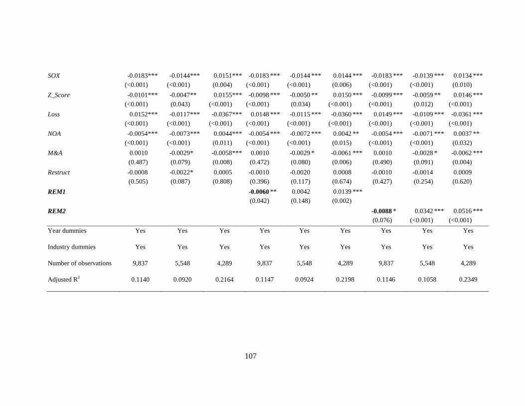
107

SOX -0.0183

(<0.001)

***

-0.0144

(<0.001)

***

0.0151

(0.004)

***

-0.0183

(<0.001)

*** -0.0144

(<0.001)

*** 0.0144

(0.006)

*** -0.0183

(<0.001)

*** -0.0139

(<0.001)

*** 0.0134

(0.010)

***

Z_Score -0.0101

(<0.001)

***

-0.0047

(0.043)

**

0.0155

(<0.001)

***

-0.0098

(<0.001)

*** -0.0050

(0.034)

** 0.0150

(<0.001)

*** -0.0099

(<0.001)

*** -0.0059

(0.012)

** 0.0146

(<0.001)

***

Loss 0.0152

(<0.001)

***

-0.0117

(<0.001)

***

-0.0367

(<0.001)

***

0.0148

(<0.001)

*** -0.0115

(<0.001)

*** -0.0360

(<0.001)

*** 0.0149

(<0.001)

*** -0.0109

(<0.001)

*** -0.0361

(<0.001)

***

NOA -0.0054

(<0.001)

***

-0.0073

(<0.001)

***

0.0044

(0.011)

***

-0.0054

(<0.001)

*** -0.0072

(<0.001)

*** 0.0042

(0.015)

** -0.0054

(<0.001)

*** -0.0071

(<0.001)

*** 0.0037

(0.032)

**

M&A 0.0010

(0.487)

-0.0029

(0.079)

*

-0.0058

(0.008)

***

0.0010

(0.472)

-0.0029

(0.080)

* -0.0061

(0.006)

*** 0.0010

(0.490)

-0.0028

(0.091)

* -0.0062

(0.004)

***

Restruct -0.0008

(0.505)

-0.0022

(0.087)

*

0.0005

(0.808)

-0.0010

(0.396)

-0.0020

(0.117)

0.0008

(0.674)

-0.0010

(0.427)

-0.0014

(0.254)

0.0009

(0.620)

REM1 -0.0060

(0.042)

** 0.0042

(0.148)

0.0139

(0.002)

***

REM2 -0.0088

(0.076)

* 0.0342

(<0.001)

*** 0.0516

(<0.001)

***

Year dummies Yes Yes Yes Yes Yes Yes Yes Yes Yes

Industry dummies Yes Yes Yes Yes Yes Yes Yes Yes Yes


Adjusted R2 0.1140 0.0920 0.2164 0.1147 0.0924 0.2198 0.1146 0.1058 0.2349

108



This table reports the results of pooled OLS regression with REM_PROD, REM_DISX, REM_CFO, REM1 and REM2 as each dependent variable. The main

variable of interest is Lagged_Rat_Diff_Firm. I use a sample of 9,837 firm-year observations for measuring real earnings management proxies, respectively,

between 1997 and 2014. I use robust standard errors clustered at the firm level. All continuous variables are winsorized at the 1% and 99% levels. The p-values are

in parentheses. ***, **, and * denote the statistical significance at the 1 percent, 5 percent, and 10 percent levels, respectively (two-tailed test). All variables are



Explanatory variables REM_PROD

(1)

REM_DISX

(2)

REM_CFO

(3)

REM1

(4)

REM2

(5)

REM_PROD

(6)

REM_DISX

(7)

REM_CFO

(8)

REM1

(9)

REM2

(10)

Intercept -0.0570

(0.030)

**

-0.0623

(0.063)

* 0.0082

(0.511)

-0.1200

(0.033)

** -0.0586

(0.091)

* -0.0569

(0.033)

** -0.0450

(0.184)

0.0024

(0.844)

-0.1036

(0.069)

* -0.0493

(0.160)

Lagged_Rat_Diff_Firm 0.0022

(<0.001)

***

0.0013

(0.042)

**

0.0007

(0.003)

***

0.0036

(0.001)

*** 0.0020

(0.003)

*** 0.0022

(<0.001)

*** 0.0013

(0.049)

** 0.0007

(0.003)

*** 0.0035

(0.002)

*** 0.0020

(0.004)

***

Size 0.0071

(0.011)

**

0.0022

(0.536)

-0.0015

(0.172)

0.0094

(0.110)

0.0012

(0.740)

0.0071

(0.011)

** 0.0017

(0.620)

-0.0013

(0.219)

0.0090

(0.126)

0.0010

(0.790)

Leverage 0.1543

(<0.001)

***

0.1880

(<0.001)

***

0.0716

(<0.001)

*** 0.3401

(<0.001)

*** 0.2572

(<0.001)

*** 0.1543

(<0.001)

*** 0.1846

(<0.001)

*** 0.0727

(<0.001)

*** 0.3368

(<0.001)

*** 0.2553

(<0.001)

***

MTB -0.0015

(<0.001)

***

-0.0021

(<0.001)

***

-0.0005

(0.001)

***

-0.0036

(<0.001)

*** -0.0027

(<0.001)

*** -0.0015

(<0.001)

*** -0.0021

(<0.001)

*** -0.0005

(0.001)

*** -0.0036

(<0.001)

*** -0.0026

(<0.001)

***

ROA -0.6853

(<0.001)

***

-0.2160

(<0.001)

*** -0.3480

(<0.001)

***

-0.8815

(<0.001)

*** -0.5354

(<0.001)

*** -0.6853

(0.001)

*** -0.2234

(<0.001)

*** -0.3455

(<0.001)

*** -0.8886

(<0.001)

*** -0.5394

(<0.001)

***

Firm_Age 0.0020

(0.789)

0.0086

(0.361)

0.0046

(0.035)

**

0.0095

(0.530)

0.0122

(0.190)

0.0020

(0.789)

0.0079

(0.402)

0.0049

(0.027)

** 0.0088

(0.559)

0.0118

(0.203)

109

Big4 0.0006

(0.939)

-0.0017

(0.866)

0.0011

(0.743)

-0.0017

(0.917)

-0.0014

(0.887)

0.0006

(0.938)

-0.0012

(0.905)

0.0009

(0.781)

-0.0012

(0.940)

-0.0012

(0.908)

SOX -0.0007

(0.920)

-0.0006

(0.937)

0.0055

(0.115)

-0.0017

(0.897)

0.0044

(0.599)

-0.0007

(0.919)

-0.0037

(0.627)

0.0065

(0.060)

* -0.0046

(0.725)

0.0027

(0.744)

Z_Score 0.0292

(<0.001)

***

0.0267

(0.002)

***

0.0030

(0.311)

0.0555

(<0.001)

*** 0.0290

(0.001)

*** 0.0292

(<0.001)

*** 0.0250

(0.003)

*** 0.0036

(0.229)

0.0539

(<0.001)

*** 0.0281

(0.001)

***

Loss -0.0352

(<0.001)

***

-0.0395

(<0.001)

***

0.0003

(0.896)

-0.0733

(<0.001)

*** -0.0366

(<0.001)

*** -0.0352

(<0.001)

*** -0.0369

(<0.001)

*** -0.0006

(0.808)

-0.0708

(<0.001)

*** -0.0352

(<0.001)

***

NOA -0.0178

(0.003)

***

0.0168

(0.018)

**

-0.0150

(<0.001)

***

-0.0021

(0.862)

0.0012

(0.866)

-0.0178

(0.003)

*** 0.0159

(0.025)

** -0.0147

(<0.001)

*** -0.0030

(0.807)

0.0007

(0.919)

M&A 0.0139

(0.013)

**

-0.0070

(0.297)

0.0064

(0.001)

***

0.0059

(0.603)

-0.0006

(0.929)

0.0139

(0.013)

** -0.0068

(0.307)

0.0063

(0.001)

*** 0.0060

(0.593)

-0.0005

(0.940)

Restruct -0.0169

(0.001)

***

-0.0206

(0.002)

***

0.0025

(0.168)

-0.0369

(0.001)

-0.0179

(0.008)

*** -0.0169

(0.001)

*** -0.0207

(0.002)

*** 0.0025

(0.159)

-0.0371

(0.001)

*** -0.0180

(0.008)

***

ABS_DA -0.0005

(0.988)

-0.1663

(0.001)

*** 0.0553

(0.008)

*** -0.1577

(0.035)

** -0.0899

(0.068)

*

Year dummies Yes Yes Yes Yes Yes Yes Yes Yes Yes Yes

Industry dummies Yes Yes Yes Yes Yes Yes Yes Yes Yes Yes

Number of observations 9,837 9,837 9,837 9,837 9,837 9,837 9,837 9,837 9,837 9,837

Adjusted R2 0.1918 0.0812 0.3017 0.1299 0.1649 0.1917 0.0839 0.3032 0.1306 0.1655

110



This table reports the results of pooled OLS regression with REM_PROD, REM_DISX, REM_CFO, REM1 and REM2 as each dependent variable. The main

variable of interest is Lagged_Rat_Diff_Ind. I use a sample of 9,837 firm-year observations for real earnings management measures, respectively, between 1997

and 2014. I use robust standard errors clustered at the firm level. All continuous variables are winsorized at the 1% and 99% levels. The p-values are in parentheses.

***, **, and * denote the statistical significance at the 1 percent, 5 percent, and 10 percent levels, respectively (two-tailed test). All variables are defined in

Appendix B.



(1)

REM_DISX

(2)

REM_CFO

(3)

REM1

(4)

REM2

(5)

REM_PROD

(6)

REM_DISX

(7)

REM_CFO

(8)

REM1

(9)

REM2

(10)

Intercept -0.0482

(0.062)

*

-0.0540

(0.096)

* 0.0091

(0.456)

-0.1031

(0.060)

* -0.0493

(0.145)

-0.0482

(0.065)

* -0.0368

(0.264)

0.0033

(0.786)

-0.0868

(0.118)

-0.0401

(0.241)

Lagged_Rat_Diff_Ind 0.0019

(<0.001)

***

0.0009

(0.141)

0.0008

(<0.001)

***

0.0029

(0.006)

*** 0.0017

(0.010)

** 0.0020

(<0.001)

*** 0.0008

(0.163)

0.0008

(<0.001)

*** 0.0028

(0.007)

*** 0.0017

(0.011)

**

Size 0.0060

(0.027)

**

0.0012

(0.733)

-0.0016

(0.126)

0.0074

(0.201)

0.0001

(0.982)

0.0060

(0.028)

** 0.0007

(0.829)

-0.0014

(0.166)

0.0070

(0.227)

-0.0002

(0.966)

Leverage 0.1584

(<0.001)

***

0.1896

(<0.001)

***

0.0733

(<0.001)

*** 0.3458

(<0.001)

*** 0.2606

(<0.001)

*** 0.1584

(<0.001)

*** 0.1860

(<0.001)

*** 0.0745

(<0.001)

*** 0.3424

(<0.001)

*** 0.2587

(<0.001)

***

MTB -0.0015

(<0.001)

***

-0.0021

(<0.001)

***

-0.0005

(0.001)

***

-0.0036

(<0.001)

*** -0.0027

(<0.001)

*** -0.0015

(<0.001)

*** -0.0021

(<0.001)

*** -0.0005

(0.001)

*** -0.0036

(<0.001)

*** -0.0026

(<0.001)

***

ROA -0.6854

(<0.001)

***

-0.2170

(<0.001)

*** -0.3474

(<0.001)

***

-0.8825

(<0.001)

*** -0.5358

(<0.001)

*** -0.6854

(<0.001)

*** -0.2245

(<0.001)

*** -0.3449

(<0.001)

*** -0.8896

(<0.001)

*** -0.5399

(<0.001)

***

Firm_Age 0.0012

(0.868)

0.0080

(0.395)

0.0045

(0.040)

**

0.0081

(0.590)

0.0114

(0.217)

0.0012

(0.867)

0.0072

(0.438)

0.0048

(0.031)

** 0.0075

(0.620)

0.0110

(0.232)

111

Big4 0.0005

(0.945)

-0.0016

(0.869)

0.0010

(0.755)

-0.0017

(0.915)

-0.0015

(0.885)

0.0005

(0.945)

-0.0012

(0.907)

0.0009

(0.794)

-0.0012

(0.938)

-0.0012

(0.906)

SOX 0.0001

(0.986)

0.0006

(0.931)

0.0053

(0.128)

0.0003

(0.981)

0.0054

(0.512)

0.0001

(0.985)

-0.0024

(0.747)

0.0063

(0.068)

* -0.0026

(0.844)

0.0038

(0.647)

Z_Score 0.0285

(<0.001)

***

0.0262

(0.002)

***

0.0028

(0.343)

0.0544

(<0.001)

*** 0.0283

(0.001)

*** 0.0285

(<0.001)

*** 0.0245

(0.003)

*** 0.0034

(0.254)

0.0528

(<0.001)

*** 0.0274

(0.001)

***

Loss -0.0345

(<0.001)

***

-0.0391

(<0.001)

***

0.0005

(0.828)

-0.0722

(<0.001)

*** -0.0360

(<0.001)

*** -0.0345

(<0.001)

*** -0.0365

(<0.001)

*** -0.0004

(0.870)

-0.0698

(<0.001)

*** -0.0346

(<0.001)

***

NOA -0.0181

(0.003)

***

0.0166

(0.020)

**

-0.0150

(<0.001)

***

-0.0026

(0.833)

0.0010

(0.892)

-0.0181

(0.003)

*** 0.0157

(0.027)

** -0.0147

(<0.001)

*** -0.0034

(0.779)

0.0005

(0.945)

M&A 0.0137

(0.015)

**

-0.0072

(0.283)

0.0063

(0.001)

***

0.0054

(0.632)

-0.0009

(0.900)

0.0137

(0.015)

** -0.0070

(0.293)

0.0062

(0.001)

*** 0.0056

(0.621)

-0.0008

(0.910)

Restruct -0.0168

(0.002)

***

-0.0205

(0.002)

***

0.0025

(0.170)

-0.0367

(0.001)

*** -0.0178

(0.009)

*** -0.0168

(0.002)

*** -0.0206

(0.002)

*** 0.0025

(0.161)

-0.0369

(0.001)

*** -0.0179

(0.008)

***

ABS_DA 0.0006

(0.988)

-0.1665

(0.001)

*** 0.0561

(0.007)

*** -0.1568

(0.037)

** -0.0892

(0.071)

*

Year dummies Yes Yes Yes Yes Yes Yes Yes Yes Yes Yes

Industry dummies Yes Yes Yes Yes Yes Yes Yes Yes Yes Yes


Adjusted R2 0.1914 0.0805 0.3027 0.1291 0.1644 0.1913 0.0832 0.3043 0.1298 0.1649

112


(Testing H1 using TEM1) (CHAPTER 5)

This table reports the results of pooled OLS regression with TEM1 as a dependent variable. To examine the effect of ratings conservatism on overall earnings

management, I follow Chan et al. (2015) and construct two measures, TEM1 and TEM2. The TEM1 is the sum of the signed discretionary accruals (DA) and the

aggregate real earnings management (REM1). The main variable of interest is Lagged_Rat_Diff_Firm and Lagged_Rat_Diff_Ind. I use robust standard errors

clustered at the firm level. All continuous variables are winsorized at the 1% and 99% level s. The p-values are in parentheses. ***, **, and * denote the statistical

significance at the 1 percent, 5 percent, and 10 percent levels, respectively (two-tailed test). All variables are defined in Appendix B.

Dependent variable: TEM1

Explanatory variables (1) (2) (3) (4) (5) (6) (7) (8)

Intercept 0.0621

(<0.001)

***

0.0699

(0.189)

0.0642

(0.236)

-0.0161

(0.774)

0.0588

(<0.001)

*** 0.0798

(0.126)

0.0743

(0.160)

0.0007

(0.990)


(<0.001)

***

0.0027

(0.011)

**

0.0027

(0.013)

** 0.0033

(0.003)

***


(<0.001)

*** 0.0023

(0.020)

** 0.0023

(0.025)

** 0.0026

(0.013)

**

Size 0.0019

(0.724)

0.0021

(0.703)

0.0068

(0.245)

0.0006

(0.911)

0.0008

(0.890)

0.0048

(0.404)

Leverage 0.2065

(<0.001)

***

0.2098

(<0.001)

*** 0.3194

(<0.001)

*** 0.2116

(<0.001)

*** 0.2147

(<0.001)

*** 0.3244

(<0.001)

***

MTB -0.0033

(<0.001)

***

-0.0033

(<0.001)

*** -0.0034

(<0.001)

*** -0.0033

(<0.001)

-0.0033

(<0.001)

*** -0.0034

(<0.001)

***

ROA -0.8782

(<0.001)

*** -0.8880

(<0.001)

*** -0.9264

(<0.001)

*** -0.8795

(<0.001)

*** -0.8892

(<0.001)

*** -0.9276

(<0.001)

***

Firm_Age 0.0015

(0.923)

0.0017

(0.909)

0.0052

(0.731)

0.0004

(0.981)

0.0006

(0.967)

0.0039

(0.797)

113

Big4 0.0035

(0.834)

0.0032

(0.849)

0.0012

(0.938)

0.0032

(0.847)

0.0030

(0.858)

0.0012

(0.939)

SOX -0.0080

(0.370)

-0.0194

(0.146)

-0.0202

(0.133)

-0.0070

(0.428)

-0.0178

(0.179)

-0.0180

(0.175)

Z_Score 0.0500

(<0.001)

***

0.0501

(<0.001)

*** 0.0454

(0.002)

*** 0.0489

(0.001)

*** 0.0490

(0.001)

*** 0.0443

(0.002)

***

Loss -0.0497

(<0.001)

***

-0.0494

(<0.001)

*** -0.0579

(<0.001)

*** -0.0490

(<0.001)

*** -0.0487

(<0.001)

*** -0.0569

(<0.001)

***

NOA 0.0017

(0.887)

0.0010

(0.936)

-0.0075

(0.539)

0.0013

(0.911)

0.0006

(0.961)

-0.0080

(0.515)

M&A 0.0109

(0.279)

0.0163

(0.141)

0.0069

(0.544)

0.0106

(0.293)

0.0158

(0.155)

0.0064

(0.571)

Restruct -0.0198

(0.067)

*

-0.0191

(0.088)

* -0.0377

(0.001)

*** -0.0201

(0.063)

* -0.0194

(0.084)

* -0.0375

(0.001)

***

Year dummies No No Yes Yes No No Yes Yes

Industry dummies No No No Yes No No No Yes

Number of observations 9,856 9,837 9,837 9,837 9,856 9,837 9,837 9,837

Adjusted R2 0.0135 0.1087 0.1091 0.1419 0.0072 0.1084 0.1087 0.1410

114


(Testing H1 using TEM2) (CHAPTER 5)

This table reports the results of pooled OLS regression with TEM2 as dependent variables. As in Table 10, I generate an overall earnings management proxy,

TEM2. The TEM2 is the sum of the signed discretionary accruals (DA) and the aggregate real earnings management (REM2).The main variable of interest is

Lagged_Rat_Diff_Firm and Lagged_Rat_Diff_Ind. I use robust standard errors clustered at the firm level. All continuous variables are winsorized at the 1% and

99% level s. The p-values are in parentheses. ***, **, and * denote the statistical significance at the 1 percent, 5 percent, and 10 percent levels, respectively (two-

tailed test). All variables are defined in Appendix B.



Intercept 0.0568

(<0.001)

***

0.1095

(0.001)

*** 0.1016

(0.003)

*** 0.0453

(0.192)

0.0542

(<0.001)

*** 0.1145

(<0.001)

*** 0.1066

(0.001)

*** 0.0544

(0.109)


(<0.001)

***

0.0015

(0.025)

**

0.0014

(0.033)

** 0.0018

(0.011)

**


(<0.001)

*** 0.0013

(0.035)

** 0.0012

(0.049)

** 0.0014

(0.034)

**

Size -0.0046

(0.178)

-0.0046

(0.186)

-0.0014

(0.693)

-0.0053

(0.116)

-0.0053

(0.122)

-0.0025

(0.476)

Leverage 0.1477

(<0.001)

***

0.1492

(<0.001)

*** 0.2365

(<0.001)

*** 0.1506

(<0.001)

*** 0.1519

(<0.001)

*** 0.2392

(<0.001)

***

MTB -0.0024

(<0.001)

***

-0.0023

(<0.001)

*** -0.0025

(<0.001)

*** -0.0024

(<0.001)

-0.0023

(<0.001)

*** -0.0025

(<0.001)

***

ROA -0.5466

(<0.001)

*** -0.5547

(<0.001)

*** -0.5803

(<0.001)

*** -0.5472

(<0.001)

*** -0.5552

(<0.001)

*** -0.5810

(<0.001)

***

Firm_Age 0.0050

(0.592)

0.0050

(0.591)

0.0079

(0.399)

0.0044

(0.634)

0.0045

(0.632)

0.0072

(0.442)

115

Big4 0.0030

(0.792)

0.0031

(0.784)

0.0015

(0.888)

0.0028

(0.803)

0.0030

(0.792)

0.0015

(0.889)

SOX -0.0108

(0.060)

*

-0.0133

(0.127)

-0.0141

(0.108)

-0.0104

(0.069)

* -0.0126

(0.146)

-0.0129

(0.137)

Z_Score 0.0218

(0.014)

**

0.0218

(0.014)

** 0.0188

(0.033)

** 0.0212

(0.017)

** 0.0212

(0.017)

** 0.0182

(0.039)

**

Loss -0.0154

(0.029)

**

-0.0148

(0.036)

** -0.0213

(0.002)

*** -0.0150

(0.033)

** -0.0144

(0.041)

** -0.0208

(0.002)

***

NOA 0.0032

(0.662)

0.0027

(0.716)

-0.0042

(0.573)

0.0030

(0.680)

0.0025

(0.735)

-0.0044

(0.551)

M&A 0.0043

(0.489)

0.0079

(0.248)

0.0004

(0.956)

0.0041

(0.508)

0.0076

(0.265)

0.0001

(0.984)

Restruct -0.0068

(0.315)

-0.0056

(0.422)

-0.0187

(0.006)

*** -0.0070

(0.302)

-0.0058

(0.410)

-0.0186

(0.007)

***




Adjusted R2 0.0195 0.1383 0.1399 0.1845 0.0094 0.1381 0.1397 0.1839

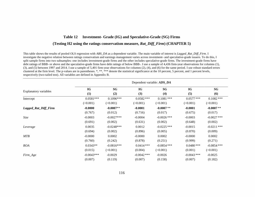
116



This table shows the results of pooled OLS regression with ABS_DA as a dependent variable. The main variable of interest is Lagged_Rat_Diff_Firm. I

investigate the negative relation between ratings conservatism and earnings management varies across investment- and speculative-grade issuers. To do this, I

split sample firms into two subsamples: one includes investment-grade firms and the other includes speculative-grade firms. The investment-grade firms have

debt ratings of BBB- or above and the speculative-grade firms have debt ratings of below BBB-. I use a sample of 4,436 firm-year observations for columns (1),

(3), and (5) between 1997 and 2014. I use a sample of 5,401 firm-year observations for columns (2), (4), and (6) for the same period. I use robust standard errors

clustered at the firm level. The p-values are in parentheses. *, **, *** denote the statistical significance at the 10 percent, 5 percent, and 1 percent levels,

respectively (two-tailed test). All variables are defined in Appendix B.

Dependent variable: ADS_DA

Explanatory variables IG

(1)

SG

(2)

IG

(3)

SG

(4)

IG

(5)

SG

(6)

Intercept 0.0581

(<0.001)

*** 0.1096

(<0.001)

*** 0.0582

(<0.001)

*** 0.1081

(<0.001)

*** 0.0577

(<0.001)

*** 0.1082

(<0.001)

***


(0.767)

-0.0007

(0.012)

**

-0.0001

(0.716)

-0.0007

(0.017)

** -0.0001

(0.675)

-0.0007

(0.017)

**

Size -0.0003

(0.691)

-0.0027

(0.002)

***

-0.0004

(0.631)

-0.0026

(0.002)

*** -0.0003

(0.648)

-0.0027

(0.002)

***

Leverage 0.0035

(0.694)

-0.0248

(0.002)

***

0.0012

(0.896)

-0.0225

(0.005)

*** -0.0015

(0.870)

-0.0211

(0.009)

***

MTB -0.0000

(0.760)

0.0002

(0.242)

-0.0000

(0.878)

0.0002

(0.251)

-0.0000

(0.999)

0.0002

(0.271)

ROA 0.0343

(0.015)

** -0.0816

(<0.001)

*** 0.0414

(0.004)

*** -0.0854

(<0.001)

*** 0.0480

(0.001)

*** -0.0854

(<0.001)

***

Firm_Age -0.0043

(0.007)

*** -0.0029

(0.119)

-0.0042

(0.007)

*** -0.0026

(0.158)

-0.0043

(0.007)

*** -0.0025

(0.182)

117

Big4 -0.0017

(0.666)

0.0056

(0.056)

* -0.0015

(0.686)

0.0056

(0.058)

* -0.0015

(0.692)

0.0055

(0.063)

*

SOX 0.0091

(0.024)

** -0.0196

(<0.001)

*** 0.0092

(0.023)

** -0.0194

(<0.001)

*** 0.0093

(0.022)

** -0.0195

(<0.001)

***

Z_Score -0.0003

(0.947)

-0.0099

(<0.001)

*** -0.0007

(0.874)

-0.0098

(<0.001)

*** -0.0010

(0.823)

-0.0099

(<0.001)

***

Loss 0.0239

(<0.001)

***

0.0095

(<0.001)

***

0.0242

(<0.001)

***

0.0092

(0.001)

***

0.0245

(<0.001)

***

0.0094

(<0.001)

***

NOA -0.0045

(<0.001)

*** -0.0059

(0.001)

*** -0.0044

(0.001)

*** -0.0056

(0.001)

*** -0.0044

(0.001)

*** -0.0056

(0.001)

***

M&A -0.0000

(0.977)

0.0005

(0.829)

-0.0001

(0.965)

0.0005

(0.839)

-0.0001

(0.973)

0.0003

(0.880)

Restruct -0.0010

(0.430)

-0.0002

(0.933)

-0.0008

(0.535)

-0.0004

(0.825)

-0.0006

(0.618)

-0.0004

(0.850)

REM1 0.0042

(0.205)

-0.0117

(0.009)

***

REM2 0.0129

(0.023)

**

-0.0216

(0.004)

***

Year dummies Yes Yes Yes Yes Yes Yes

Industry dummies Yes Yes Yes Yes Yes Yes

Number of observations 4,436 5,401 4,436 5,401 4,436 5,401

Adjusted R2 0.1043 0.0983 0.1048 0.1002 0.1067 0.1009

Test of equal coefficients for

Rat_Diff_Firm between investment-

and speculative-grade subsamples

2 = 4.45 (p-value = 0.035)

2 = 3.88 (p-value = 0.049)

2 = 3.79 (p-value = 0.052)

118



This table shows the results of pooled OLS regression with ABS_DA as a dependent variable. The main variable of interest is Lagged_Rat_Diff_Ind. I

investigate the negative relation between ratings conservatism and earnings management varies across investment- and speculative-grade issuers. To do this, I

split sample firms into two subsamples: one includes investment-grade firms and the other includes speculative-grade firms. The investment-grade firms have

debt ratings of BBB- or above and the speculative-grade firms have debt ratings of below BBB-. I use a sample of 4,436 firm-year observations for columns (1),

(3), and (5) between 1997 and 2014. I use a sample of 5,401 firm-year observations for columns (2), (4), and (6) for the same period. I use robust standard errors

clustered at the firm level. The p-values are in parentheses. *, **, *** denote the statistical significance at the 10 percent, 5 percent, and 1 percent levels,

respectively (two-tailed test). All variables are defined in Appendix B.

Dependent variable: ADS_DA


(1)

SG

(2)

IG

(3)

SG

(4)

IG

(5)

SG

(6)

Intercept 0.0580

(<0.001)

*** 0.1069

(<0.001)

*** 0.0580

(<0.001)

*** 0.1057

(<0.001)

*** 0.0575

(<0.001)

*** 0.1057

(<0.001)

***


(0.791)

-0.0009

(0.001)

***

-0.0000

(0.744)

-0.0009

(0.002)

*** -0.0000

(0.698)

-0.0009

(0.002)

***

Size -0.0003

(0.703)

-0.0023

(0.008)

***

-0.0003

(0.645)

-0.0023

(0.009)

*** -0.0003

(0.664)

-0.0023

(0.007)

***

Leverage 0.0035

(0.700)

-0.0264

(0.001)

***

0.0011

(0.902)

-0.0240

(0.003)

*** -0.0016

(0.863)

-0.0226

(0.005)

***

MTB -0.0000

(0.758)

0.0002

(0.243)

-0.0000

(0.876)

0.0002

(0.251)

-0.0000

(0.999)

0.0002

(0.271)

ROA 0.0344

(0.015)

** -0.0827

(<0.001)

*** 0.0414

(0.004)

*** -0.0864

(<0.001)

*** 0.0481

(0.001)

*** -0.0864

(<0.001)

***

Firm_Age -0.0043

(0.007)

*** -0.0028

(0.133)

-0.0042

(0.008)

*** -0.0025

(0.173)

-0.0043

(0.007)

*** -0.0024

(0.199)

119

Big4 -0.0017

(0.666)

0.0056

(0.055)

* -0.0015

(0.686)

0.0056

(0.058)

* -0.0015

(0.692)

0.0055

(0.062)

*

SOX -0.0144

(<0.001)

*** -0.0193

(<0.001)

*** -0.0143

(<0.001)

*** -0.0190

(<0.001)

*** -0.0142

(<0.001)

*** -0.0192

(<0.001)

***

Z_Score -0.0003

(0.948)

-0.0097

(<0.001)

*** -0.0007

(0.875)

-0.0096

(<0.001)

*** -0.0009

(0.824)

-0.0097

(<0.001)

***

Loss 0.0239

(<0.001)

***

0.0093

(0.001)

***

0.0242

(<0.001)

***

0.0090

(0.001)

***

0.0244

(<0.001)

***

0.0092

(<0.001)

***

NOA -0.0045

(<0.001)

*** -0.0059

(<0.001)

*** -0.0044

(0.001)

*** -0.0056

(0.001)

*** -0.0044

(0.001)

*** -0.0056

(0.001)

***

M&A -0.0000

(0.977)

0.0006

(0.777)

-0.0001

(0.965)

0.0006

(0.789)

-0.0001

(0.973)

0.0005

(0.830)

Restruct -0.0010

(0.430)

-0.0002

(0.902)

-0.0008

(0.534)

-0.0005

(0.796)

-0.0006

(0.617)

-0.0004

(0.820)

REM1 0.0042

(0.206)

-0.0116

(0.010)

***

REM2 0.0129

(0.023)

**

-0.0215

(0.004)

***




Adjusted R2 0.1043 0.0994 0.1048 0.1013 0.1067 0.1020


Rat_Diff_Firm between investment-

and speculative-grade subsamples

2 = 8.37 (p-value = 0.004)

2 = 7.69 (p-value = 0.006)

2 = 7.61 (p-value = 0.006)

120


(Testing H2 using REM1) (CHAPTER 5)

This table shows the results of pooled OLS regression with REM1 as a dependent variable. The main variable of interest is Lagged_Rat_Diff_Firm and

Lagged_Rat_Diff_Ind. I investigate the negative relation between ratings conservatism and earnings management varies across investment- and speculative-

grade issuers. To do this, I split sample firms into two subsamples: one includes investment-grade firms and the other includes speculative-grade firms. The

investment-grade firms have debt ratings of BBB- or above and the speculative-grade firms have debt ratings of below BBB-. I use a sample of 4,436 firm-year

observations for columns (1), (3), (5), and (7) between 1997 and 2014. I use a sample of 5,401 firm-year observations for columns (2), (4), (6), and (8) for the

same period. I use robust standard errors clustered at the firm level. The p-values are in parentheses. *, **, *** denote the statistical significance at the 10

percent, 5 percent, and 1 percent levels, respectively (two-tailed test). All variables are defined in Appendix B.

Dependent variable: REM1


(1)

SG

(2)

IG

(3)

SG

(4)

IG

(5)

SG

(6)

IG

(7)

SG

(8)

Intercept -0.0186

(0.871)

-0.1218

(0.043)

*** -0.0298

(0.798)

-0.1004

(0.095)

* -0.0102

(0.928)

-0.1108

(0.063)

* -0.0213

(0.853)

-0.0900

(0.131)


(0.151)

0.0032

(0.042)

**

0.0022

(0.149)

0.0031

(0.050)

**


(0.185)

0.0028

(0.081)

* 0.0018

(0.183)

0.0027

(0.098)

*

Size 0.0154

(0.127)

0.0045

(0.471)

0.0154

(0.126)

0.0040

(0.523)

0.0143

(0.149)

0.0033

(0.597)

0.0143

(0.148)

0.0029

(0.647)

Leverage 0.5511

(<0.001)

***

0.2000

(<0.001)

***

0.5504

(<0.001)

*** 0.1951

(<0.001)

*** 0.5544

(<0.001)

*** 0.2038

(<0.001)

*** 0.5537

(<0.001)

*** 0.1987

(<0.001)

***

MTB -0.0059

(<0.001)

***

-0.0004

(0.640)

-0.0059

(<0.001)

*** -0.0003

(0.675)

-0.0059

(<0.001)

-0.0004

(0.648)

-0.0059

(<0.001)

*** -0.0003

(0.683)

ROA -1.6922

(<0.001)

*** -0.3242

(<0.001)

*** -1.6988

(<0.001)

*** -0.3401

(<0.001)

*** -1.6942

(<0.001)

*** -0.3208

(<0.001)

*** -1.7008

(<0.001)

*** -0.3368

(<0.001)

***

121

Firm_Age -0.0101

(0.681)

0.0234

(0.153)

-0.0093

(0.705)

0.0228

(0.163)

-0.0109

(0.659)

0.0228

(0.162)

-0.0101

(0.682)

0.0223

(0.173)

Big4 -0.0247

(0.435)

-0.0013

(0.937)

-0.0244

(0.442)

-0.0002

(0.989)

-0.0246

(0.437)

-0.0015

(0.931)

-0.0243

(0.443)

-0.0004

(0.982)

SOX -0.0227

(0.290)

0.0200

(0.173)

-0.0245

(0.260)

0.0162

(0.274)

-0.0304

(0.212)

0.0208

(0.156)

-0.0276

(0.249)

0.0170

(0.248)

Z_Score 0.0947

(<0.001)

***

0.0093

(0.498)

0.0947

(<0.001)

*** 0.0073

(0.591)

0.0945

(<0.001)

***

0.0083

(0.544)

0.0945

(<0.001)

*** 0.0064

(0.638)

Loss -0.0778

(<0.001)

***

-0.0244

(0.020)

**

-0.0824

(<0.001)

*** -0.0226

(0.030)

** -0.0776

(<0.001)

***

-0.0235

(0.025)

** -0.0822

(<0.001)

*** -0.0217

(0.037)

**

NOA -0.0287

(0.110)

0.0208

(0.121)

-0.0279

(0.121)

0.0197

(0.142)

-0.0288

(0.108)

0.0204

(0.129)

-0.0280

(0.119)

0.0192

(0.150)

M&A 0.0060

(0.724)

-0.0024

(0.847)

0.0060

(0.724)

-0.0023

(0.853)

0.0060

(0.723)

-0.0033

(0.790)

0.0060

(0.723)

-0.0031

(0.798)

Restruct -0.0528

(0.001)

***

-0.0221

(0.109)

-0.0526

(0.001)

*** -0.0221

(0.108)

-0.0528

(0.001)

***

-0.0218

(0.114)

-0.0526

(0.001)

*** -0.0219

(0.113)

ABS_DA 0.1920

(0.219)

-0.1957

(0.008)

*** 0.1917

(0.220)

-0.1945

(0.008)

***

Year dummies Yes Yes Yes Yes Yes Yes Yes Yes

Industry dummies Yes Yes Yes Yes Yes Yes Yes Yes


Adjusted R2 0.2838 0.0858 0.2842 0.0877 0.2836 0.0854 0.2840 0.0873


Rat_Diff_Firm (Rat_Diff_Ind)

between investment- and

speculative-grade subsamples

2 = 0.21 (p-value = 0.647)

2 = 0.16 (p-value = 0.694)

2 = 0.27 (p-value = 0.603)

2 = 0.19 (p-value = 0.662)

122


(Testing H2 using REM2) (CHAPTER 5)

This table shows the results of pooled OLS regression with REM2 as dependent variables. The main variable of interest is Lagged_Rat_Diff_Firm and

Lagged_Rat_Diff_Ind. I investigate the negative relation between ratings conservatism and earnings management varies across investment- and speculative-

grade issuers. To do this, I split sample firms into two subsamples: one includes investment-grade firms and the other includes speculative-grade firms. The

investment-grade firms have debt ratings of BBB- or above and the speculative-grade firms have debt ratings of below BBB-. I use a sample of 4,436 firm-year

observations for columns (1), (3), (5), and (7) between 1997 and 2014. I use a sample of 5,401 firm-year observations for columns (2), (4), (6), and (8) for the

same period. I use robust standard errors clustered at the firm level. The p-values are in parentheses. *, **, *** denote the statistical significance at the 10

percent, 5 percent, and 1 percent levels, respectively (two-tailed test). All variables are defined in Appendix B.

Dependent variable: REM2


(1)

SG

(2)

IG

(3)

SG

(4)

IG

(5)

SG

(6)

IG

(7)

SG

(8)

Intercept 0.0328

(0.637)

-0.0628

(0.093)

* 0.0196

(0.782)

-0.0471

(0.206)

0.0356

(0.605)

-0.0566

(0.123)

0.0224

(0.749)

-0.0413

(0.259)


(0.176)

0.0018

(0.062)

*

0.0013

(0.171)

0.0017

(0.075)

*


(0.173)

0.0015

(0.127)

0.0011

(0.168)

0.0014

(0.157)

Size 0.0034

(0.567)

-0.0013

(0.743)

0.0035

(0.558)

-0.0017

(0.670)

0.0030

(0.608)

-0.0019

(0.615)

0.0030

(0.599)

-0.0023

(0.556)

Leverage 0.3907

(<0.001)

***

0.1739

(<0.001)

***

0.3899

(<0.001)

*** 0.1704

(<0.001)

*** 0.3929

(<0.001)

*** 0.1759

(<0.001)

*** 0.3922

(<0.001)

*** 0.1722

(<0.001)

***

MTB -0.0039

(<0.001)

***

-0.0006

(0.213)

-0.0039

(<0.001)

*** -0.0006

(0.233)

-0.0039

(<0.001)

-0.0006

(0.218)

-0.0038

(<0.001)

*** -0.0006

(0.239)

ROA -1.0632

(<0.001)

*** -0.1766

(0.001)

*** -1.0710

(<0.001)

*** -0.1883

(<0.001)

*** -1.0640

(<0.001)

*** -0.1747

(0.001)

*** -1.0719

(<0.001)

*** -0.1865

(<0.001)

***

123

Firm_Age 0.0002

(0.992)

0.0201

(0.046)

** 0.0011

(0.940)

0.0197

(0.051)

* -0.0002

(0.990)

0.0198

(0.049)

** 0.0008

(0.959)

0.0194

(0.054)

*

Big4 -0.0111

(0.551)

-0.0038

(0.736)

-0.0107

(0.564)

-0.0030

(0.790)

-0.0111

(0.552)

-0.0039

(0.731)

-0.0107

(0.565)

-0.0031

(0.785)

SOX -0.0101

(0.441)

0.0039

(0.686)

-0.0122

(0.356)

0.0011

(0.912)

-0.0165

(0.270)

0.0044

(0.642)

-0.0133

(0.373)

0.0017

(0.861)

Z_Score 0.0523

(0.002)

***

0.0003

(0.973)

0.0524

(0.002)

*** -0.0011

(0.891)

0.0523

(0.002)

***

-0.0003

(0.975)

0.0523

(0.002)

*** -0.0016

(0.843)

Loss -0.0446

(<0.001)

***

-0.0036

(0.577)

-0.0500

(<0.001)

*** -0.0022

(0.728)

-0.0445

(<0.001)

***

-0.0031

(0.632)

-0.0500

(<0.001)

*** -0.0018

(0.784)

**

NOA -0.0137

(0.203)

0.0144

(0.071)

*

-0.0127

(0.238)

0.0135

(0.089)

* -0.0137

(0.202)

0.0141

(0.076)

* -0.0127

(0.237)

0.0133

(0.094)

*

M&A 0.0007

(0.947)

-0.0067

(0.376)

0.0007

(0.946)

-0.0067

(0.380)

0.0007

(0.945)

-0.0072

(0.339)

0.0007

(0.945)

-0.0071

(0.344)

Restruct -0.0292

(0.001)

***

-0.0092

(0.279)

-0.0290

(0.002)

*** -0.0092

(0.277)

-0.0292

(0.001)

***

-0.0091

(0.287)

-0.0290

(0.002)

-0.0091

(0.284)

ABS_DA 0.2272

(0.027)

** -0.1434

(0.003)

*** 0.2271

(0.027)

** -0.1429

(0.003)

***

Year dummies Yes Yes Yes Yes Yes Yes Yes Yes

Industry dummies Yes Yes Yes Yes Yes Yes Yes Yes


Adjusted R2 0.3089 0.1106 0.3108 0.1132 0.3089 0.1102 0.3108 0.1128


Rat_Diff_Firm (Rat_Diff_Ind)

between investment- and

speculative-grade subsamples

2 = 0.16 (p-value = 0.691)

2 = 0.10 (p-value = 0.750)

2 = 0.11 (p-value = 0.741)

2 = 0.05 (p-value = 0.819)

124

Table 16 Potential Sample Selection Bias



is Lagged_Rat_Diff_Firm. I use a sample of 9,837, 5,548, and 4,289 firm-year observations for ABS_DA, Positive_DA, and Negative_DA, respectively, between

1997 and 2014. I use robust standard errors clustered at the firm level. All continuous variables are winsorized at the 1% and 99% levels. The p-values are in

parentheses. ***, **, and * denote the statistical significance at the 1 percent, 5 percent, and 10 percent levels, respectively (two-tailed test).


Key explanatory variables ABS_DA

(1)

Positive_DA

(2)

Negative_DA

(3)

ABS_DA

(4)

Positive_DA

(5)

Negative_DA

(6)


(0.038)

** -0.0000

(0.890)

0.0004

(0.020)

** -0.0002

(0.032)

** -0.0001

(0.414)

0.0003

(0.064)

*

REM1 -0.0068

(0.020)

** 0.0044

(0.133)

0.0159

(<0.001)

***

REM2 -0.0119

(0.014)

** 0.0345

(<0.001)

*** 0.0580

(<0.001)

***

IMR -0.0030

(0.936)

0.0260

(0.497)

0.0108

(0.823)

0.0204

(0.426)

-0.0051

(0.843)

-0.0483

(0.171)

Control variables and Intercept Yes Yes Yes Yes Yes Yes




Adjusted R2 0.1240 0.0971 0.2320 0.1243 0.1106 0.2509

125

Table 16 (Continued) Potential Sample Selection Bias



is Lagged_Rat_Diff_Ind. I use a sample of 9,837, 5,548, and 4,289 firm-year observations for ABS_DA, Positive_DA, and Negative_DA, respectively, between

1997 and 2014. I use robust standard errors clustered at the firm level. All continuous variables are winsorized at the 1% and 99% level s. The p-values are in



Key explanatory variables ABS_DA

(1)

Positive_DA

(2)

Negative_DA

(3)

ABS_DA

(4)

Positive_DA

(5)

Negative_DA

(6)


(0.042)

** -0.0001

(0.277)

0.0003

(0.095)

* -0.0002

(0.040)

** -0.0002

(0.076)

* 0.0002

(0.223)

REM1 -0.0069

(0.019)

** 0.0045

(0.117)

0.0162

(<0.001)

***

REM2 -0.0121

(0.014)

** 0.0347

(<0.001)

*** 0.0584

(<0.001)

***

IMR 0.0040

(0.914)

0.0228

(0.553)

0.0111

(0.820)

0.0194

(0.453)

-0.0055

(0.832)

-0.0473

(0.184)





Adjusted R2 0.1240 0.0973 0.2315 0.1242 0.1110 0.2505

126

Table 16 (Continued) Potential Sample Selection Bias

(Testing H1 using two ratings conservatism proxies) (CHAPTER 6)

This table reports the results of pooled OLS regression with REM1 and REM2 as each dependent variable. The main variable of interest is

Lagged_Rat_Diff_Firm and Lagged_Rat_Diff_Ind. I use a sample of 9,837 firm-year observations between 1997 and 2014. I use robust standard errors clustered

at the firm level. All continuous variables are winsorized at the 1% and 99% level s. The p-values are in parentheses. ***, **, and * denote the statistical

significance at the 1 percent, 5 percent, and 10 percent levels, respectively (two-tailed test).


Key explanatory variables REM1

(1)

REM2

(2)

REM1

(3)

REM2

(4)


(0.004)

*** 0.0019

(0.003)

***


(0.025)

** 0.0015

(0.017)

**

ABS_DA -0.2060

(0.006)

*** -0.1349

(0.006)

*** -0.2073

(0.006)

*** -0.1357

(0.006)

***

IMR 0.1219

(0.617)

0.1771

(0.113)

0.1052

(0.665)

0.1803

(0.107)

Control variables and Intercept Yes Yes Yes Yes

Year dummies Yes Yes Yes Yes

Industry dummies Yes Yes Yes Yes

Number of observations 9,837 9,837 9,837 9,837

Adjusted R2 0.1174 0.1490 0.1162 0.1481

127


Relation between Ratings Conservatism and Earnings Smoothing (CHAPTER 7)

This table reports the results of pooled OLS regression with EM_SMOOTH1, EM_SMOOTH2, and EM_SMOOTH3 as each dependent variable. The main

variable of interest is Lagged_Rat_Diff_Firm and Lagged_Rat_Diff_Ind. I use a sample of 8,553, 8,534, and 8,453 firm-year observations for EM_SMOOTH1,

EM_SMOOTH2, and EM_SMOOTH3, respectively, between 1997 and 2014. I use robust standard errors clustered at the firm level. All continuous variables are

winsorized at the 1% and 99% levels. The p-values are in parentheses. ***, **, and * denote the statistical significance at the 1 percent, 5 percent, and 10 percent

levels, respectively (two-tailed test).


Key explanatory variables EM_SMOOTH1 EM_SMOOTH2 EM_SMOOTH3

(1) (2) (3) (4) (5) (6)


(0.741)

-0.0007

(0.503)

-0.0006

(0.540)


(0.436)

0.0000

(0.968)

0.0004

(0.661)





Adjusted R2 0.0691 0.0692 0.0366 0.0365 0.0526 0.0526

128

Table 17 (Continued) Additional Analysis

Descriptive Statistics (CHAPTER 7)

This table shows descriptive statistics for earnings smoothing measures in equations (10)-(12). My sample period is between 1997 and 2014. All

variables are defined in Appendix B.

Variable N Mean Std. Dev. Median Minimum Maximum

σ(Earnings)/σ(CFO) 9,981 1.7280 2.6982 0.8790 0.0604 18.2320

ρ(∆ACC, ∆CFO) 9,962 -0.5343 0.6218 -0.8702 -1.0000 1.0000

ρ(∆DA, ∆PDI) 9,874 -0.5798 0.6110 -0.9063 -1.0000 1.0000

129


Relation between Ratings Conservatism and Asymmetric Timely Loss Recognition (CHAPTER 7)

This table reports the results of pooled OLS regression with NI, ACC, and C_Score as each dependent variable. I use a sample of 12,199, 11,509, and 11,147

firm-year observations for NI, ACC, and C_Score, respectively, between 1997 and 2014. I use robust standard errors clustered at the firm level. All continuous

variables are winsorized at the 1% and 99% levels. The p-values are in parentheses. ***, **, and * denote the statistical significance at the 1 percent, 5 percent, and

10 percent levels, respectively (two-tailed test).


Key explanatory variables NI ACC C_Score

(1) (2) (3) (4) (5) (6)

D*RET*Lagged_Rat_Diff_Firm 0.0785

(0.430)

D*RET*Lagged_Rat_Diff_Ind 0.0213

(0.817)

DCFO*CFO*Lagged_Rat_Diff_Firm -0.0009

(0.968)

DCFO*CFO*Lagged_Rat_Diff_Ind 0.0414

(0.005)

***


(0.096)

*


(0.017)

**





Adjusted R2 0.0907 0.0936 0.3259 0.3275 0.4733 0.4734

130

Table 19

Alternative Measures of Accrual-Based Earnings Management 1: Testing H1 (CHAPTER 8)

This table reports the results of pooled OLS regression with ABS_DA, Positive_DA, and Negative_DA as each dependent variable. I repeat my tests using a measure

based on discretionary accruals proposed by Cohen et al. (2008). I use robust standard errors clustered at the firm level. All continuous variables are winsorized at the 1%

and 99% levels. The p-values are in parentheses. ***, **, and * denote the statistical significance at the 1 percent, 5 percent, and 10 percent levels, respectively (two-tailed

test).



(1)

Positive_DA

(2)

Negative_DA

(3)

ABS_DA

(4)

Positive_DA

(5)

Negative_DA

(6)

ABS_DA

(7)

Positive_DA

(8)

Negative_DA

(9)


(0.042)

**

-0.0000

(0.797)

0.0004

(0.024)

**

-0.0002

(0.065)

* -0.0000

(0.724)

0.0004

(0.049)

** -0.0002

(0.054)

* -0.0001

(0.456)

0.0003

(0.092)

*

REM1 -0.0054

(0.064)

* 0.0044

(0.134)

0.0134

(0.003)

***

REM2 -0.0075

(0.096)

* 0.0346

(<0.001)

*** 0.0508

(<0.001)

***

Control variables and Intercept Yes Yes Yes Yes Yes Yes Yes Yes Yes

Year and Industry dummies Yes Yes Yes Yes Yes Yes Yes Yes Yes


Adjusted R2 0.1136 0.0919 0.2186 0.1142 0.0924 0.2217 0.1140 0.1061 0.2368



(1)

Positive_DA

(2)

Negative_DA

(3)

ABS_DA

(4)

Positive_DA

(5)

Negative_DA

(6)

ABS_DA

(7)

Positive_DA

(8)

Negative_DA

(9)


(0.009)

***

-0.0002

(0.114)

0.0004

(0.035)

**

-0.0003

(0.013)

** -0.0002

(0.091)

* 0.0003

(0.058)

* -0.0003

(0.012)

** -0.0002

(0.035)

** 0.0003

(0.093)

*

REM1 -0.0053

(0.067)

* 0.0046

(0.117)

0.0135

(0.003)

***

REM2 -0.0075

(0.092)

* 0.0350

(<0.001)

*** 0.0509

(<0.001)

***


Year/Industry dummies Yes Yes Yes Yes Yes Yes Yes Yes Yes


Adjusted R2 0.1139 0.0924 0.2184 0.1145 0.0929 0.2217 0.1143 0.1068 0.2368

131

Table 19 (Continued)


This table reports the results of pooled OLS regression with REM_PROD, REM_DISX, REM_CFO, REM1 and REM2 as each dependent variable. I repeat my

tests using a measure based on discretionary accruals proposed by Cohen et al. (2008). I use robust standard errors clustered at the firm level. All continuous





(1)

REM_DISX

(2)

REM_CFO

(3)

REM1

(4)

REM2

(5)

REM_PROD

(6)

REM_DISX

(7)

REM_CFO

(8)

REM1

(9)

REM2

(10)


(<0.001)

***

0.0013

(0.042)

**

0.0007

(0.003)

***

0.0036

(0.001)

*** 0.0020

(0.003)

** 0.0022

(<0.001)

*** 0.0013

(0.049)

** 0.0007

(0.003)

*** 0.0035

(0.002)

*** 0.0020

(0.004)

***

ABS_DA 0.0097

(0.784)

-0.1569

(0.001)

*** 0.0618

(0.003)

*** -0.1397

(0.059)

* -0.0764

(0.094)

*

Control variables and Intercept Yes Yes Yes Yes Yes Yes Yes Yes Yes Yes

Year/Industry dummies Yes Yes Yes Yes Yes Yes Yes Yes Yes Yes


Adjusted R2 0.1918 0.0812 0.3017 0.1299 0.1649 0.1917 0.0836 0.3036 0.1305 0.1653



(1)

REM_DISX

(2)

REM_CFO

(3)

REM1

(4)

REM2

(5)

REM_PROD

(6)

REM_DISX

(7)

REM_CFO

(8)

REM1

(9)

REM2

(10)


(<0.001)

***

0.0009

(0.141)

0.0008

(<0.001)

***

0.0029

(0.006)

*** 0.0017

(0.010)

** 0.0020

(<0.001)

*** 0.0008

(0.162)

0.0008

(<0.001)

*** 0.0028 (0.007)

*** 0.0017 (0.011)

**

ABS_DA 0.0108

(0.762)

-0.1572

(0.001)

*** 0.0626

(0.003)

*** -0.1388

(0.061)

* -0.0758

(0.093)

*




Adjusted R2 0.1914 0.0805 0.3027 0.1291 0.1644 0.1913 0.0829 0.3047 0.1296 0.1648

132



This table reports the results of pooled OLS regression with TEM1 and TEM2 as each dependent variable. I repeat my tests using a measure based on discretionary

accruals proposed by Cohen et al. (2008). I use robust standard errors clustered at the firm level. All continuous variables are winsorized at the 1% and 99% levels. The p-

values are in parentheses. ***, **, and * denote the statistical significance at the 1 percent, 5 percent, and 10 percent levels, respectively (two-tailed test).



Lagged_Rat_Diff_Firm 0.0057 (<0.001)

***

0.0027 (0.011)

**

0.0027

(0.013)

** 0.0033

(0.003)

***


(<0.001)

*** 0.0023

(0.020)

** 0.0023

(0.026)

** 0.0026

(0.014)

**

Intercept Yes Yes Yes Yes Yes Yes Yes Yes

Control variables No Yes Yes Yes No Yes Yes Yes




Adjusted R2 0.0135 0.1084 0.1087 0.1420 0.0072 0.1080 0.1084 0.1411




(<0.001)

***

0.0015

(0.025)

**

0.0014

(0.035)

** 0.0018

(0.011)

**


(<0.001)

*** 0.0013

(0.036)

** 0.0012

(0.051)

* 0.0014

(0.035)

**






Adjusted R2 0.0194 0.1376 0.1392 0.1845 0.0093 0.1375 0.1390 0.1840

133

Table 20


This table reports the results of pooled OLS regression with ABS_DA, Positive_DA, and Negative_DA as each dependent variable. I repeat my tests using a measure based on

discretionary accruals proposed by Chen et al. (2008) and Francis and Yu (2009). I use robust standard errors clustered at the firm level. All continuous variables are winsorized at

the 1% and 99% levels. The p-values are in parentheses. ***, **, and * denote the statistical significance at the 1 percent, 5 percent, and 10 percent levels, respectively (two-tailed

test).



(1)

Positive_DA

(2)

Negative_DA

(3)

ABS_DA

(4)

Positive_DA

(5)

Negative_DA

(6)

ABS_DA

(7)

Positive_DA

(8)

Negative_DA

(9)


(0.081)

*

0.0001

(0.496)

0.0005

(0.010)

***

-0.0002

(0.090)

* 0.0001

(0.549)

0.0004

(0.019)

** -0.0002

(0.087)

* 0.0000

(0.808)

0.0004

(0.033)

**

REM1 -0.0054

(0.058)

* 0.0040

(0.170)

0.0116

(0.007)

***

REM2 -0.0081

(0.090)

* 0.0325

(<0.001)

*** 0.0460

(<0.001)

***




Adjusted R2 0.1177 0.0982 0.2174 0.1183 0.0986 0.2198 0.1182 0.1106 0.2332



(1)

Positive_DA

(2)

Negative_DA

(3)

ABS_DA

(4)

Positive_DA

(5)

Negative_DA

(6)

ABS_DA

(7)

Positive_DA

(8)

Negative_DA

(9)


(0.018)

**

-0.0001

(0.463)

0.0004

(0.015)

**

-0.0002

(0.024)

** -0.0001

(0.411)

0.0004

(0.025)

** -0.0002

(0.023)

** -0.0001

(0.239)

0.0003

(0.035)

**

REM1 -0.0054

(0.061)

* 0.0042

(0.151)

0.0117

(0.007)

***

REM2 -0.0080

(0.094)

* 0.0329

(<0.001)

*** 0.0462

(<0.001)

***




Adjusted R2 0.1180 0.0983 0.2172 0.1186 0.0987 0.2197 0.1185 0.1109 0.2332

134



This table reports the results of pooled OLS regression with REM_PROD, REM_DISX, REM_CFO, REM1 and REM2 as each dependent variable. I repeat my

tests using a measure based on discretionary accruals proposed by Chen et al. (2008) and Francis and Yu (2009). I use robust standard errors clustered at the

firm level. All continuous variables are winsorized at the 1% and 99% levels. The p-values are in parentheses. ***, **, and * denote the statistical significance at

the 1 percent, 5 percent, and 10 percent levels, respectively (two-tailed test).



(1)

REM_DISX

(2)

REM_CFO

(3)

REM1

(4)

REM2

(5)

REM_PROD

(6)

REM_DISX

(7)

REM_CFO

(8)

REM1

(9)

REM2

(10)


(<0.001)

***

0.0013

(0.042)

**

0.0007

(0.003)

***

0.0036

(0.001)

*** 0.0020

(0.003)

*** 0.0022

(<0.001)

*** 0.0013

(0.047)

** 0.0007

(0.003)

*** 0.0035

(0.002)

*** 0.0020

(0.004)

***

ABS_DA 0.0107

(0.766)

-0.1625

(0.001)

*** 0.0596

(0.005)

*** -0.1440

(0.053)

* -0.0843

(0.085)

*




Adjusted R2 0.1918 0.0812 0.3017 0.1299 0.1649 0.1917 0.0837 0.3034 0.1305 0.1654



(1)

REM_DISX

(2)

REM_CFO

(3)

REM1

(4)

REM2

(5)

REM_PROD

(6)

REM_DISX

(7)

REM_CFO

(8)

REM1

(9)

REM2

(10)


(<0.001)

***

0.0009

(0.141)

0.0008

(<0.001)

***

0.0029

(0.006)

*** 0.0017

(0.010)

*** 0.0020

(<0.001)

*** 0.0008

(0.159)

0.0008

(<0.001)

*** 0.0028

(0.007)

*** 0.0017

(0.011)

**

ABS_DA 0.0119

(0.741)

-0.1626

(0.001)

*** 0.0604

(0.005)

*** -0.1428

(0.056)

* -0.0835

(0.089)

*




Adjusted R2 0.1914 0.0805 0.3027 0.1291 0.1644 0.1913 0.0830 0.3045 0.1296 0.1648

135



This table reports the results of pooled OLS regression with TEM1 and TEM2 as each dependent variable. I repeat my tests using a measure based on discretionary

accruals proposed by Chen et al. (2008) and Francis and Yu (2009). I use robust standard errors clustered at the firm level. All continuous variables are winsorized at the

1% and 99% level s. The p-values are in parentheses. ***, **, and * denote the statistical significance at the 1 percent, 5 percent, and 10 percent levels, respectively (two

tailed test).




(<0.001)

***

0.0028

(0.009)

***

0.0027

(0.012)

** 0.0034

(0.003)

***


(<0.001)

*** 0.0024

(0.018)

** 0.0023

(0.023)

** 0.0026

(0.012)

**






Adjusted R2 0.0140 0.1090 0.1093 0.1432 0.0075 0.1086 0.1090 0.1423




(<0.001)

***

0.0015

(0.019)

**

0.0015

(0.027)

** 0.0018

(0.008)

***


(<0.001)

*** 0.0013

(0.028)

** 0.0013

(0.041)

** 0.0014

(0.027)

**






Adjusted R2 0.0204 0.1392 0.1408 0.1873 0.0099 0.1391 0.1406 0.1867

136

Table 21


This table reports the results of pooled OLS regression with ABS_PMDA, Positive_PMDA, and Negative_PMDA as each dependent variable. I repeat my tests using the

performance-matched discretionary accruals proposed by Kothari et al. (2005). I use robust standard errors clustered at the firm level. All continuous variables are

winsorized at the 1% and 99% levels. The p-values are in parentheses. ***, **, and * denote the statistical significance at the 1 percent, 5 percent, and 10 percent levels,

respectively (two-tailed test).


Explanatory variables ABS_PMDA

(1)

Positive_PMDA

(2) Negative_PMDA

(3)

ABS_PMDA

(4)

Positive_PMDA

(5)

Negative_PMDA

(6)

ABS_PMDA

(7)

Positive_PMDA

(8)

Negative_PMDA

(9)


(0.488)

0.0002

(0.359)

0.0004 (0.030)

**

-0.0001

(0.629)

0.0002

(0.293)

0.0004 (0.043)

** -0.0001

(0.643)

0.0002

(0.384)

0.0004 (0.071)

*

REM1 -0.0103

(0.004)

*** -0.0101

(0.022)

** 0.0089

(0.071)

*

REM2 -0.0191

(0.001)

*** 0.0051

(0.464)

0.0403

(<0.001)

***




Adjusted R2 0.0843 0.0819 0.1028 0.0854 0.0829 0.1036 0.0858 0.0819 0.1104


Explanatory variables ABS_PMDA

(1)

Positive_PMDA

(2) Negative_PMDA

(3)

ABS_PMDA

(4)

Positive_PMDA

(5)

Negative_PMDA

(6)

ABS_PMDA

(7)

Positive_PMDA

(8)

Negative_PMDA

(9)


(0.082)

*

-0.0001

(0.786)

0.0004 (0.019)

**

-0.0002

(0.117)

-0.0000

(0.881)

0.0004 (0.025)

** -0.0002

(0.122)

-0.0001

(0.755)

0.0004 (0.039)

**

REM1 -0.0102

(0.004)

*** -0.0098

(0.026)

** 0.0089

(0.069)

*

REM2 -0.0189

(0.001)

*** 0.0056

(0.428)

0.0403

(<0.001)

***




Adjusted R2 0.0845 0.0818 0.1029 0.0856 0.0827 0.1037 0.0860 0.0817 0.1106

137



This table reports the results of pooled OLS regression with ABS_PMDA, Positive_PMDA, and Negative_PMDA as each dependent variable. I repeat my tests

using the performance-matched discretionary accruals proposed by Kothari et al. (2005). I use robust standard errors clustered at the firm level. All continuous





(1)

REM_DISX

(2)

REM_CFO

(3)

REM1

(4)

REM2

(5)

REM_PROD

(6)

REM_DISX

(7)

REM_CFO

(8)

REM1

(9)

REM2

(10)


(<0.001)

***

0.0013

(0.042)

**

0.0007

(0.003)

***

0.0036

(0.001)

*** 0.0020

(0.003)

*** 0.0019

(<0.001)

*** 0.0009

(0.047)

0.0007

(0.001)

*** 0.0028

(0.005)

*** 0.0016

(0.008)

***

ABS_PMDA -0.0277

(0.206)

-0.1048

(<0.001)

*** 0.0005

(0.966)

-0.1283

(0.004)

*** -0.0928

(0.001)

***




Adjusted R2 0.1918 0.0812 0.3017 0.1299 0.1649 0.1935 0.0876 0.2995 0.1360 0.1710



(1)

REM_DISX

(2)

REM_CFO

(3)

REM1

(4)

REM2

(5)

REM_PROD

(6)

REM_DISX

(7)

REM_CFO

(8)

REM1

(9)

REM2

(10)


(<0.001)

***

0.0009

(0.141)

0.0008

(<0.001)

***

0.0029

(0.006)

*** 0.0017

(0.010)

*** 0.0017

(<0.001)

*** 0.0005

(0.352)

0.0008

(<0.001)

*** 0.0023

(0.020)

** 0.0013

(0.025)

**

ABS_PMDA -0.0264

(0.227)

-0.1046

(<0.001)

*** 0.0011

(0.920)

-0.1268

(0.004)

*** -0.0920

(0.001)

***




Adjusted R2 0.1914 0.0805 0.3027 0.1291 0.1644 0.1930 0.0871 0.3003 0.1352 0.1704

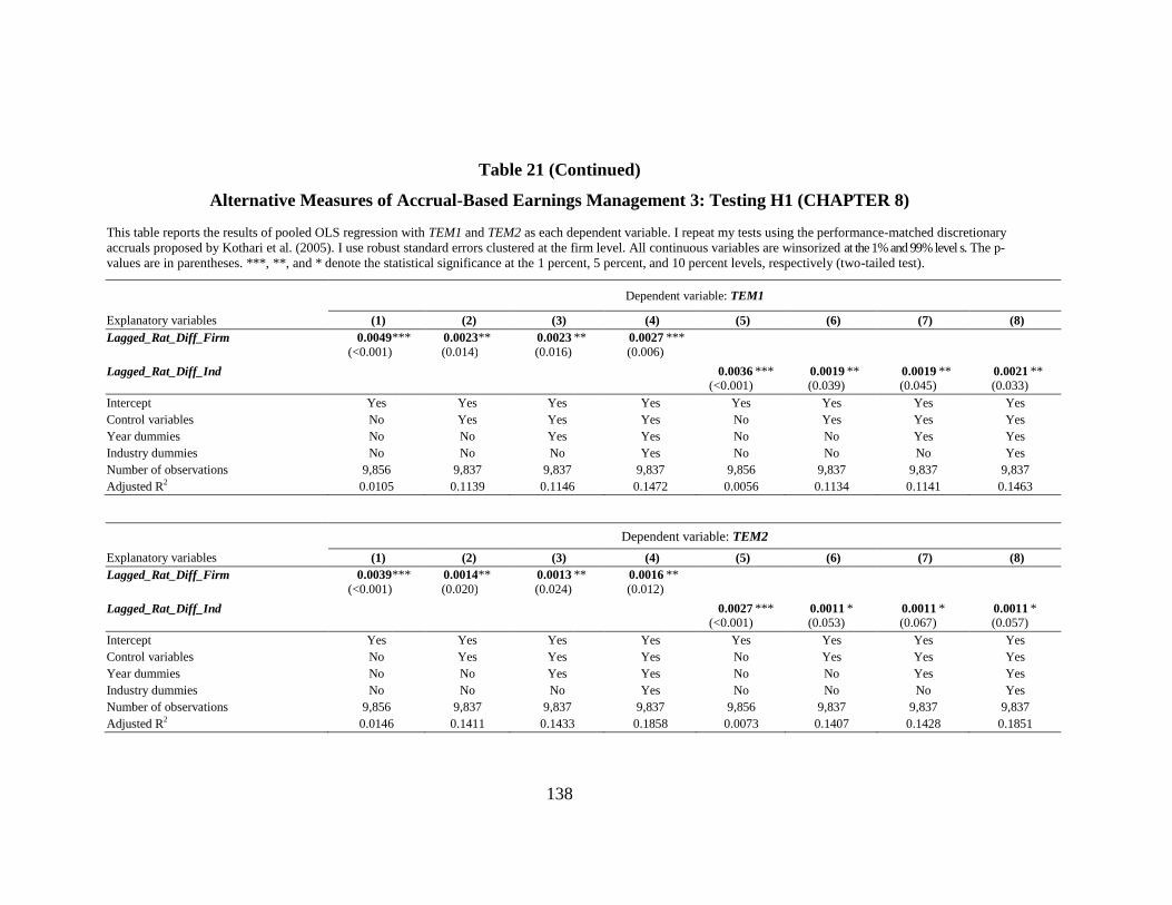
138



This table reports the results of pooled OLS regression with TEM1 and TEM2 as each dependent variable. I repeat my tests using the performance-matched discretionary

accruals proposed by Kothari et al. (2005). I use robust standard errors clustered at the firm level. All continuous variables are winsorized at the 1% and 99% level s. The p-





(<0.001)

***

0.0023

(0.014)

**

0.0023

(0.016)

** 0.0027

(0.006)

***


(<0.001)

*** 0.0019

(0.039)

** 0.0019

(0.045)

** 0.0021

(0.033)

**






Adjusted R2 0.0105 0.1139 0.1146 0.1472 0.0056 0.1134 0.1141 0.1463




(<0.001)

***

0.0014

(0.020)

**

0.0013

(0.024)

** 0.0016

(0.012)

**


(<0.001)

*** 0.0011

(0.053)

* 0.0011

(0.067)

* 0.0011

(0.057)

*






Adjusted R2 0.0146 0.1411 0.1433 0.1858 0.0073 0.1407 0.1428 0.1851

139

Table 22


This table reports the results of pooled OLS regression with ABS_AWCA, Positive_AWCA, and Negative_AWCA as each dependent variable. I repeat my tests using the

abnormal working capital accruals proposed by Dechow and Dichev (2002). I use robust standard errors clustered at the firm level. All continuous variables are




Explanatory variables ABS_AWCA

(1)

Positive_AWCA

(2) Negative_AWCA

(3)

ABS_AWCA

(4)

Positive_AWCA

(5)

Negative_AWCA

(6)

ABS_AWCA

(7) Positive_AWCA

(8)

Negative_AWCA

(9)


(<0.001)

***

-0.0001

(<0.001)

***

0.0001

(0.324)

-0.0001

(<0.001)

*** -0.0001

(<0.001)

*** 0.0001

(0.399)

-0.0001

(<0.001)

*** -0.0001

(<0.001)

*** 0.0001

(0.486)

REM1 -0.0016 (<0.001)

*** -0.0014 (<0.001)

*** 0.0032

(0.028)

**

REM2 -0.0001

(0.823)

0.0001

(0.923)

0.0096

(<0.001)

***




Adjusted R2 0.0931 0.1038 0.0154 0.0952 0.1055 0.0235 0.0930 0.1037 0.0504


Explanatory variables ABS_AWCA

(1)

Positive_AWCA

(2)

Negative_AWCA

(3)

ABS_AWCA

(4)

Positive_AWCA

(5)

Negative_AWCA

(6)

ABS_AWCA

(7)

Positive_AWCA

(8)

Negative_AWCA

(9)

Lagged_Rat_Diff_Ind -0.0001 (<0.001)

***

-0.0001

(<0.001)

***

0.0001

(0.231)

-0.0001

(<0.001)

*** -0.0001 (<0.001)

*** 0.0001

(0.270)

-0.0001

(<0.001)

*** -0.0001 (<0.001)

*** 0.0001

(0.307)

REM1 -0.0016

(<0.001)

*** -0.0014

(<0.001)

*** 0.0032

(0.028)

**

REM2 -0.0002

(0.771)

0.0000

(0.960)

0.0096

(<0.001)

***




Adjusted R2 0.0921 0.1030 0.0171 0.0943 0.1048 0.0252 0.0920 0.1030 0.0523

140



This table reports the results of pooled OLS regression with ABS_AWCA, Positive_AWCA, and Negative_AWCA as each dependent variable. I repeat my tests

using the abnormal working capital accruals proposed by Dechow and Dichev (2002). I use robust standard errors clustered at the firm level. All continuous





(1)

REM_DISX

(2)

REM_CFO

(3)

REM1

(4)

REM2

(5)

REM_PROD

(6)

REM_DISX

(7)

REM_CFO

(8)

REM1

(9)

REM2

(10)


(<0.001)

***

0.0013

(0.042)

**

0.0007

(0.003)

***

0.0036

(0.001)

*** 0.0020

(0.003)

*** 0.0016

(0.001)

*** 0.0009

(0.096)

* 0.0008

(<0.001)

*** 0.0025

(0.007)

*** 0.0017

(0.003)

***

ABS_AWCA -0.8732

(0.206)

-0.7387

(0.001)

*** 0.6565

(<0.001)

*** -1.5503

(<0.001)

*** -0.0552

(0.823)




Adjusted R2 0.1918 0.0812 0.3017 0.1299 0.1649 0.1842 0.0821 0.2725 0.1324 0.1598



(1)

REM_DISX

(2)

REM_CFO

(3)

REM1

(4)

REM2

(5)

REM_PROD

(6)

REM_DISX

(7)

REM_CFO

(8)

REM1

(9)

REM2

(10)


(<0.001)

***

0.0009

(0.141)

0.0008

(<0.001)

***

0.0029

(0.006)

*** 0.0017

(0.010)

*** 0.0015

(0.001)

*** 0.0007

(0.201)

0.0008

(<0.001)

*** 0.0022

(0.017)

** 0.0015

(0.008)

***

ABS_AWCA -0.8857

(0.227)

-0.7520

(0.001)

*** 0.6534

(<0.001)

*** -1.5758

(0.004)

*** -0.0719

(0.771)




Adjusted R2 0.1914 0.0805 0.3027 0.1291 0.1644 0.1838 0.0817 0.2729 0.1319 0.1593

141



This table reports the results of pooled OLS regression with TEM1 and TEM2 as each dependent variable. I repeat my tests using the abnormal working capital accruals

proposed by Dechow and Dichev (2002). I use robust standard errors clustered at the firm level. All continuous variables are winsorized at the 1% and 99% level s. The p-





(<0.001)

***

0.0023

(0.011)

**

0.0022

(0.014)

** 0.0026

(0.006)

***


(<0.001)

*** 0.0021

(0.017)

** 0.0020

(0.020)

** 0.0022

(0.015)

**






Adjusted R2 0.0094 0.0995 0.0996 0.1269 0.0058 0.0993 0.0994 0.1263




(<0.001)

***

0.0015

(0.007)

***

0.0014

(0.010)

*** 0.0016

(0.005)

***


(<0.001)

*** 0.0014

(0.009)

*** 0.0014

(0.013)

** 0.0014

(0.011)

**






Adjusted R2 0.0134 0.1171 0.1183 0.1531 0.0079 0.1170 0.1182 0.1527

142

Table 23

Using a Three-Digit SIC Industry: Testing H1 (CHAPTER 8)

This table reports the results of pooled OLS regression with ABS_DA, Positive_DA, and Negative_DA as each dependent variable. I repeat previous analyses by replacing

a rating proxy based on a two-digit SIC industry with a rating proxy based on a three-digit SIC industry. I use robust standard errors clustered at the firm level. All

continuous variables are winsorized at the 1% and 99% levels. The p-values are in parentheses. ***, **, and * denote the statistical significance at the 1 percent, 5 percent,

and 10 percent levels, respectively (two-tailed test).



(1)

Positive_DA

(2)

Negative_DA

(3)

ABS_DA

(4)

Positive_DA

(5)

Negative_DA

(6)

ABS_DA

(7)

Positive_DA

(8)

Negative_DA

(9)


(0.027)

**

-0.0001

(0.471)

0.0004

(0.029)

**

-0.0002

(0.040)

** -0.0001

(0.418)

0.0003

(0.056)

** -0.0002

(0.038)

** -0.0001

(0.224)

0.0003

(0.096)

*

REM1 -0.0061

(0.041)

** 0.0040

(0.167)

0.0137

(0.003)

***

REM2 -0.0088

(0.076)

* 0.0339

(<0.001)

*** 0.0513

(<0.001)

***




Adjusted R2 0.1138 0.0914 0.2167 0.1145 0.0917 0.2200 0.1144 0.1050 0.2350



(1)

Positive_DA

(2)

Negative_DA

(3)

ABS_DA

(4)

Positive_DA

(5)

Negative_DA

(6)

ABS_DA

(7)

Positive_DA

(8)

Negative_DA

(9)

Lagged_Rat_Diff_Ind_1 -0.0003

(0.010)

***

-0.0002

(0.052)

*

0.0003

(0.058)

*

-0.0003

(0.014)

** -0.0002

(0.042)

** 0.0003

(0.091)

* -0.0003

(0.014)

** -0.0003

(0.015)

** 0.0003

(0.133)

REM1 -0.0061

(0.041)

** 0.0042

(0.149)

0.0139

(0.002)

***

REM2 -0.0088

(0.077)

* 0.0342

(<0.001)

*** 0.0515

(<0.001)

***




Adjusted R2 0.1140 0.0920 0.2164 0.1147 0.0924 0.2198 0.1146 0.1058 0.2349

143



This table reports the results of pooled OLS regression with REM_PROD, REM_DISX, REM_CFO, REM1 and REM2 as each dependent variable. I repeat

previous analyses by replacing a rating proxy based on a two-digit SIC industry with a rating proxy based on a three-digit SIC industry. I use robust standard

errors clustered at the firm level. All continuous variables are winsorized at the 1% and 99% levels. The p-values are in parentheses. ***, **, and * denote the

statistical significance at the 1 percent, 5 percent, and 10 percent levels, respectively (two-tailed test).



(1)

REM_DISX

(2)

REM_CFO

(3)

REM1

(4)

REM2

(5)

REM_PROD

(6)

REM_DISX

(7)

REM_CFO

(8)

REM1

(9)

REM2

(10)


(<0.001)

***

0.0012

(0.047)

**

0.0007

(0.001)

***

0.0032

(0.002)

*** 0.0019

(0.003)

*** 0.0020

(<0.001)

*** 0.0011

(0.055)

* 0.0007

(0.001)

*** 0.0031

(0.002)

*** 0.0019

(0.003)

***

ABS_DA -0.0002

(0.996)

-0.1661

(0.001)

*** 0.0560

(0.008)

*** -0.1571

(0.036)

** -0.0890

(0.071)

*




Adjusted R2 0.1916 0.0812 0.3019 0.1298 0.1650 0.1915 0.0838 0.3035 0.1305 0.1655



(1)

REM_DISX

(2)

REM_CFO

(3)

REM1

(4)

REM2

(5)

REM_PROD

(6)

REM_DISX

(7)

REM_CFO

(8)

REM1

(9)

REM2

(10)

Lagged_Rat_Diff_Ind_1 0.0018

(<0.001)

***

0.0007

(0.203)

0.0008

(0.001)

***

0.0025

(0.010)

*** 0.0015

(0.013)

** 0.0018

(<0.001)

*** 0.0007

(0.232)

0.0008

(0.001)

*** 0.0025

(0.011)

** 0.0015

(0.015)

**

ABS_DA 0.0003

(0.993)

-0.1669

(0.001)

*** 0.0566

(0.007)

** -0.1574

(0.036)

** -0.0891

(0.072)

*




Adjusted R2 0.1911 0.0803 0.3029 0.1287 0.1641 0.1910 0.0830 0.3045 0.1294 0.1647

144



This table reports the results of pooled OLS regression with TEM1 and TEM2 as each dependent variable. I repeat previous analyses by replacing a rating proxy based on

a two-digit SIC industry with a rating proxy based on a three-digit SIC industry. I use robust standard errors clustered at the firm level. All continuous variables are






(<0.001)

***

0.0025

(0.010)

***

0.0025

(0.012)

** 0.0029

(0.004)

***


(<0.001)

*** 0.0022

(0.024)

** 0.0021

(0.030)

** 0.0023

(0.022)

**






Adjusted R2 0.0117 0.1088 0.1091 0.1417 0.0062 0.1083 0.1086 0.1407




(<0.001)

***

0.0015

(0.017)

**

0.0014

(0.023)

** 0.0016

(0.011)

**


(<0.001)

*** 0.0013

(0.033)

** 0.0012

(0.046)

** 0.0013

(0.044)

**






Adjusted R2 0.0164 0.1385 0.1401 0.1845 0.0083 0.1382 0.1398 0.1854

145

Table 24

Alternative Cut-Off Years (1985-1997): Testing H1 (CHAPTER 8)

This table reports the results of pooled OLS regression with ABS_DA, Positive_DA, and Negative_DA as each dependent variable. I use alternative cut-off years for

measuring ratings conservatism. To predict ratings for the period 1998 to 2014, I employ the ratings model estimated for the period 1985 to 1997. I use robust standard

errors clustered at the firm level. All continuous variables are winsorized at the 1% and 99% levels. The p-values are in parentheses. ***, **, and * denote the statistical




(1)

Positive_DA

(2)

Negative_DA

(3)

ABS_DA

(4)

Positive_DA

(5)

Negative_DA

(6)

ABS_DA

(7)

Positive_DA

(8)

Negative_DA

(9)


(0.061)

*

-0.0000

(0.811)

0.0004

(0.052)

*

-0.0002

(0.090)

* -0.0000

(0.718)

0.0003

(0.105)

-0.0002

(0.089)

* -0.0001

(0.440)

0.0003

(0.178)

REM1 -0.0064

(0.029)

** 0.0052

(0.067)

* 0.0153

(0.001)

***

REM2 -0.0104

(0.035)

** 0.0337

(<0.001)

*** 0.0533

(<0.001)

***




Adjusted R2 0.1157 0.1012 0.2146 0.1165 0.1019 0.2187 0.1166 0.1150 0.2343



(1)

Positive_DA

(2)

Negative_DA

(3)

ABS_DA

(4)

Positive_DA

(5)

Negative_DA

(6)

ABS_DA

(7)

Positive_DA

(8)

Negative_DA

(9)


(0.018)

**

-0.0002

(0.176)

0.0003

(0.068)

*

-0.0002

(0.028)

** -0.0002

(0.140)

0.0003

(0.126)

-0.0002

(0.028)

** -0.0002

(0.056)

* 0.0002

(0.203)

REM1 -0.0064

(0.030)

** 0.0053

(0.058)

* 0.0154

(0.001)

***

REM2 -0.0103

(0.037)

** 0.0340

(<0.001)

*** 0.0534

(<0.001)

***




Adjusted R2 0.1159 0.1015 0.2144 0.1167 0.1023 0.2186 0.1168 0.1156 0.2343

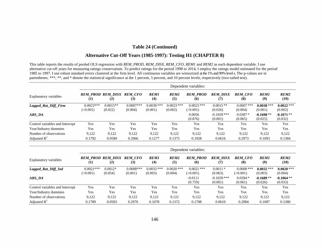
146



This table reports the results of pooled OLS regression with REM_PROD, REM_DISX, REM_CFO, REM1 and REM2 as each dependent variable. I use

alternative cut-off years for measuring ratings conservatism. To predict ratings for the period 1998 to 2014, I employ the ratings model estimated for the period

1985 to 1997. I use robust standard errors clustered at the firm level. All continuous variables are winsorized at the 1% and 99% level s. The p-values are in




(1)

REM_DISX

(2)

REM_CFO

(3)

REM1

(4)

REM2

(5)

REM_PROD

(6)

REM_DISX

(7)

REM_CFO

(8)

REM1

(9)

REM2

(10)


(<0.001)

***

0.0015

(0.022)

**

0.0007

(0.004)

***

0.0039

(0.001)

*** 0.0023

(0.002)

*** 0.0023

(<0.001)

*** 0.0015

(0.026)

** 0.0007

(0.004)

*** 0.0038

(0.001)

*** 0.0022

(0.002)

***

ABS_DA 0.0056

(0.876)

-0.1659

(0.001)

*** 0.0387

(0.065)

* -0.1698

(0.025)

** -0.1071

(0.032)

**




Adjusted R2 0.1792 0.0589 0.2966 0.1277 0.1375 0.1928 0.0616 0.2973 0.1093 0.1384



(1)

REM_DISX

(2)

REM_CFO

(3)

REM1

(4)

REM2

(5)

REM_PROD

(6)

REM_DISX

(7)

REM_CFO

(8)

REM1

(9)

REM2

(10)


(<0.001)

***

0.0012

(0.054)

*

0.0008

(0.001)

***

0.0033

(0.003)

*** 0.0020

(0.004)

*** 0.0021

(<0.001)

*** 0.0011

(0.063)

* 0.0008

(<0.001)

*** 0.0032

(0.003)

*** 0.0020

(0.004)

***

ABS_DA -0.0111

(0.759)

-0.1659

(0.001)

*** 0.0394

(0.061)

* -0.1689

(0.026)

** -0.1064

(0.033)

**




Adjusted R2 0.1789 0.0583 0.2976 0.1078 0.1372 0.1788 0.0610 0.2984 0.1087 0.1380

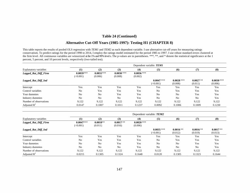
147



This table reports the results of pooled OLS regression with TEM1 and TEM2 as each dependent variable. I use alternative cut-off years for measuring ratings

conservatism. To predict ratings for the period 1998 to 2014, I employ the ratings model estimated for the period 1985 to 1997. I use robust standard errors clustered at

the firm level. All continuous variables are winsorized at the 1% and 99% level s. The p-values are in parentheses. ***, **, and * denote the statistical significance at the 1

percent, 5 percent, and 10 percent levels, respectively (two-tailed test).




(<0.001)

***

0.0031

(0.006)

***

0.0030

(0.008)

*** 0.0036

(0.002)

***


(<0.001)

*** 0.0028

(0.008)

*** 0.0027

(0.011)

** 0.0030

(0.006)

***






Adjusted R2 0.0147 0.1007 0.1011 0.1237 0.0092 0.1006 0.1009 0.1230




(<0.001)

***

0.0018

(0.011)

**

0.0017

(0.016)

** 0.0020

(0.006)

***


(<0.001)

*** 0.0016

(0.012)

** 0.0016

(0.019)

** 0.0017

(0.013)

**






Adjusted R2 0.0215 0.1305 0.1324 0.1648 0.0120 0.1305 0.1323 0.1644

148

Table 25



measuring ratings conservatism. To predict ratings for the period 1999 to 2014, I employ the ratings model estimated for the period 1985 to 1998. I use robust standard

errors clustered at the firm level. All continuous variables are winsorized at the 1% and 99% levels. The p-values are in parentheses. ***, **, and * denote the statistical




(1)

Positive_DA

(2)

Negative_DA

(3)

ABS_DA

(4)

Positive_DA

(5)

Negative_DA

(6)

ABS_DA

(7)

Positive_DA

(8)

Negative_DA

(9)


(0.129)

-0.0000

(0.940)

0.0003

(0.075)

*

-0.0002

(0.169)

-0.0000

(0.818)

0.0003

(0.128)

-0.0002

(0.172)

-0.0001

(0.495)

0.0002

(0.220)

REM1 -0.0051

(0.090)

* 0.0062

(0.035)

** 0.0132

(0.007)

***

REM2 -0.0090

(0.077)

* 0.0359

(<0.001)

*** 0.0513

(<0.001)

***




Adjusted R2 0.1159 0.0920 0.2265 0.1164 0.0931 0.2294 0.1166 0.1078 0.2440



(1)

Positive_DA

(2)

Negative_DA

(3)

ABS_DA

(4)

Positive_DA

(5)

Negative_DA

(6)

ABS_DA

(7)

Positive_DA

(8)

Negative_DA

(9)


(0.025)

**

-0.0001

(0.272)

0.0003

(0.065)

*

-0.0002

(0.037)

** -0.0002

(0.206)

0.0003

(0.114)

-0.0002

(0.038)

** -0.0002

(0.078)

* 0.0002

(0.203)

REM1 -0.0050

(0.098)

* 0.0064

(0.029)

** 0.0132

(0.006)

***

REM2 -0.0088

(0.084)

* 0.0363

(<0.001)

*** 0.0513

(<0.001)

***




Adjusted R2 0.1163 0.0923 0.2265 0.1167 0.0934 0.2294 0.1169 0.1084 0.2440

149



This table reports the results of pooled OLS regression with REM_PROD, REM_DISX, REM_CFO, REM1 and REM2 as each dependent variable. I use

alternative cut-off years for measuring ratings conservatism. To predict ratings for the period 1999 to 2014, I employ the ratings model estimated for the period

1985 to 1998. I use robust standard errors clustered at the firm level. All continuous variables are winsorized at the 1% and 99% level s. The p-values are in




(1)

REM_DISX

(2)

REM_CFO

(3)

REM1

(4)

REM2

(5)

REM_PROD

(6)

REM_DISX

(7)

REM_CFO

(8)

REM1

(9)

REM2

(10)


(<0.001)

***

0.0014

(0.022)

**

0.0007

(0.002)

***

0.0035

(0.001)

*** 0.0021

(0.002)

*** 0.0021

(<0.001)

*** 0.0014

(0.025)

** 0.0007

(0.001)

*** 0.0035

(0.001)

*** 0.0021

(0.002)

***

ABS_DA 0.0134

(0.716)

-0.1544

(0.002)

*** 0.0432

(0.048)

** -0.1334

(0.084)

* -0.0902

(0.072)

*




Adjusted R2 0.1967 0.0765 0.2991 0.1309 0.1638 0.1966 0.0788 0.3000 0.1313 0.1643



(1)

REM_DISX

(2)

REM_CFO

(3)

REM1

(4)

REM2

(5)

REM_PROD

(6)

REM_DISX

(7)

REM_CFO

(8)

REM1

(9)

REM2

(10)


(<0.001)

***

0.0014

(0.017)

**

0.0007

(0.001)

***

0.0035

(0.001)

*** 0.0021

(0.001)

*** 0.0021

(<0.001)

*** 0.0013

(0.021)

** 0.0007

(0.001)

*** 0.0035

(0.001)

*** 0.0021

(0.001)

***

ABS_DA 0.0153

(0.677)

-0.1531

(0.002)

*** 0.0439

(0.044)

** -0.1302

(0.091)

* -0.0883

(0.078)

*




Adjusted R2 0.1971 0.0766 0.2994 0.1312 0.1641 0.1971 0.0789 0.3003 0.1317 0.1646

150




conservatism. To predict ratings for the period 1999 to 2014, I employ the ratings model estimated for the period 1985 to 1998. I use robust standard errors clustered at

the firm level. All continuous variables are winsorized at the 1% and 99% level s. The p-values are in parentheses. ***, **, and * denote the statistical significance at the 1

percent, 5 percent, and 10 percent levels, respectively (two-tailed test).




(<0.001)

***

0.0028

(0.005)

***

0.0028

(0.007)

*** 0.0033

(0.002)

***


(<0.001)

*** 0.0029

(0.003)

*** 0.0029

(0.004)

** 0.0032

(0.002)

***






Adjusted R2 0.0146 0.1136 0.1144 0.1437 0.0100 0.1141 0.1148 0.1439




(<0.001)

***

0.0017

(0.009)

***

0.0016

(0.013)

** 0.0019

(0.005)

***


(<0.001)

*** 0.0017

(0.006)

*** 0.0017

(0.009)

*** 0.0019

(0.005)

***






Adjusted R2 0.0210 0.1442 0.1464 0.1853 0.0132 0.1445 0.1467 0.1854

151

Table 26

Controlling for the Effect of Global Financial Crisis of 2007-2008: Testing H1 (CHAPTER 8)


measuring ratings conservatism. I use robust standard errors clustered at the firm level. All continuous variables are winsorized at the 1% and 99% levels. The p-values are

in parentheses. ***, **, and * denote the statistical significance at the 1 percent, 5 percent, and 10 percent levels, respectively (two-tailed test).



(1)

Positive_DA

(2)

Negative_DA

(3)

ABS_DA

(4)

Positive_DA

(5)

Negative_DA

(6)

ABS_DA

(7)

Positive_DA

(8)

Negative_DA

(9)


(0.029)

**

-0.0000

(0.862)

0.0004

(0.011)

**

-0.0002

(0.041)

** -0.0000

(0.793)

0.0004

(0.022)

-0.0002

(0.039)

** -0.0001

(0.509)

0.0003

(0.041)

**

REM1 -0.0060

(0.039)

** 0.0041

(0.162)

0.0134

(0.002)

***

REM2 -0.0087

(0.072)

* 0.0347

(<0.001)

*** 0.0513

(<0.001)

***




Adjusted R2 0.1208 0.0949 0.2298 0.1216 0.0953 0.2329 0.1214 0.1090 0.2479



(1)

Positive_DA

(2)

Negative_DA

(3)

ABS_DA

(4)

Positive_DA

(5)

Negative_DA

(6)

ABS_DA

(7)

Positive_DA

(8)

Negative_DA

(9)


(0.011)

**

-0.0001

(0.192)

0.0004

(0.024)

**

-0.0002

(0.015)

** -0.0001

(0.162)

0.0003

(0.039)

** -0.0003

(0.015)

** -0.0002

(0.072)

* 0.0003

(0.062)

*

REM1 -0.0060

(0.040)

** 0.0042

(0.148)

0.0136

(0.002)

***

REM2 -0.0087

(0.073)

* 0.0349

(<0.001)

*** 0.0514

(<0.001)

***




Adjusted R2 0.1210 0.0952 0.2295 0.1218 0.0956 0.2327 0.1216 0.1095 0.2478

152



This table reports the results of pooled OLS regression with REM_PROD, REM_DISX, REM_CFO, REM1 and REM2 as each dependent variable. I use robust

standard errors clustered at the firm level. All continuous variables are winsorized at the 1% and 99% level s. The p-values are in parentheses. ***, **, and * denote

the statistical significance at the 1 percent, 5 percent, and 10 percent levels, respectively (two-tailed test).



(1)

REM_DISX

(2)

REM_CFO

(3)

REM1

(4)

REM2

(5)

REM_PROD

(6)

REM_DISX

(7)

REM_CFO

(8)

REM1

(9)

REM2

(10)


(<0.001)

***

0.0010

(0.088)

*

0.0007

(0.001)

***

0.0029

(0.003)

*** 0.0017

(0.005)

*** 0.0019

(<0.001)

*** 0.0009

(0.101)

0.0007

(0.001)

*** 0.0029

(0.004)

*** 0.0017

(0.006)

***

ABS_DA -0.0035

(0.924)

-0.1627

(<0.001)

*** 0.0557

(0.008)

*** -0.1557

(0.036)

** -0.0880

(0.068)

*




Adjusted R2 0.1922 0.0868 0.2894 0.1358 0.1691 0.1921 0.0893 0.2909 0.1365 0.1697



(1)

REM_DISX

(2)

REM_CFO

(3)

REM1

(4)

REM2

(5)

REM_PROD

(6)

REM_DISX

(7)

REM_CFO

(8)

REM1

(9)

REM2

(10)


(<0.001)

***

0.0006

(0.263)

0.0008

(<0.001)

***

0.0024

(0.012)

** 0.0014

(0.016)

** 0.0018

(<0.001)

*** 0.0006

(0.297)

0.0008

(<0.001)

*** 0.0024

(0.014)

** 0.0014

(0.018)

**

ABS_DA -0.0030

(0.935)

-0.1633

(<0.001)

*** 0.0563

(0.007)

*** -0.1557

(0.036)

** -0.0879

(0.068)

*




Adjusted R2 0.1917 0.0862 0.2903 0.1350 0.1685 0.1917 0.0888 0.2918 0.1357 0.1691

153




conservatism. I use robust standard errors clustered at the firm level. All continuous variables are winsorized at the 1% and 99% level s. The p-values are in





(<0.001)

***

0.0023

(0.015)

**

0.0023

(0.017)

** 0.0027

(0.007)

***


(<0.001)

*** 0.0020

(0.032)

** 0.0020

(0.036)

** 0.0021

(0.026)

**






Adjusted R2 0.0135 0.1132 0.1132 0.1476 0.0072 0.1128 0.1128 0.1468




(<0.001)

***

0.0013

(0.026)

**

0.0013

(0.033)

** 0.0015

(0.017)

**


(<0.001)

*** 0.0012

(0.046)

** 0.0011

(0.057)

* 0.0012

(0.051)

*






Adjusted R2 0.0195 0.1429 0.1438 0.1886 0.0094 0.1427 0.1436 0.1880

154

Table 27


This table reports the results of pooled OLS regression with ABS_DA, Positive_DA, and Negative_DA as each dependent variable. To mitigate the possibility of omitted

variable problems, I re-estimate the regression equation (8) after controlling for operating cycle (Cycle), cash flow operations (CFO), sales growth (Sales_Growth), and a

litigation indicator (LIT) as well as existing control variables employed in equation. I use robust standard errors clustered at the firm level. All continuous variables are





(1)

Positive_DA

(2)

Negative_DA

(3)

ABS_DA

(4)

Positive_DA

(5)

Negative_DA

(6)

ABS_DA

(7)

Positive_DA

(8)

Negative_DA

(9)


(0.014)

**

-0.0002

(0.188)

0.0005

(0.005)

***

-0.0003

(0.018)

** -0.0001

(0.191)

0.0004

(0.007)

*** -0.0003

(0.017)

** -0.0002

(0.169)

0.0004

(0.009)

***

REM1 -0.0054

(0.079)

* -0.0008

(0.775)

0.0079

(0.050)

**

REM2 -0.0096

(0.062)

* 0.0065

(0.166)

0.0229

(0.001)

***




Adjusted R2 0.1260 0.2615 0.3097 0.1265 0.2614 0.3106 0.1266 0.2618 0.3129



(1)

Positive_DA

(2)

Negative_DA

(3)

ABS_DA

(4)

Positive_DA

(5)

Negative_DA

(6)

ABS_DA

(7)

Positive_DA

(8)

Negative_DA

(9)


(0.004)

***

-0.0003

(0.008)

***

0.0004

(0.019)

**

-0.0003

(0.005)

*** -0.0003

(0.008)

*** 0.0003

(0.025)

** -0.0003

(0.004)

*** -0.0003

(0.006)

*** 0.0003

(0.028)

**

REM1 -0.0054

(0.078)

* -0.0007

(0.800)

0.0080

(0.045)

**

REM2 -0.0097

(0.061)

* 0.0066

(0.155)

0.0232

(0.001)

***




Adjusted R2 0.1262 0.2625 0.3092 0.1268 0.2624 0.3102 0.1269 0.2628 0.3124

155



This table reports the results of pooled OLS regression with REM_PROD, REM_DISX, REM_CFO, REM1 and REM2 as each dependent variable. To mitigate the

possibility of omitted variable problems, I re-estimate the regression equation (8) after controlling for operating cycle (Cycle), cash flow operations (CFO), sales growth

(Sales_Growth), and a litigation indicator (LIT) as well as existing control variables employed in equation. I use robust standard errors clustered at the firm level. All

continuous variables are winsorized at the 1% and 99% levels. The p-values are in parentheses. ***, **, and * denote the statistical significance at the 1 percent, 5 percent,

and 10 percent levels, respectively (two-tailed test).



(1)

REM_DISX

(2)

REM_CFO

(3)

REM1

(4)

REM2

(5)

REM_PROD

(6)

REM_DISX

(7)

REM_CFO

(8)

REM1

(9)

REM2

(10)


(0.002)

***

0.0008

(0.145)

0.0003

(0.002)

***

0.0022

(0.018)

*** 0.0012

(0.030)

** 0.0014

(0.002)

*** 0.0008

(0.163)

0.0003

(0.001)

*** 0.0022

(0.020)

** 0.0012

(0.033)

***

ABS_DA -0.0141

(0.701)

-0.1300

(0.005)

*** 0.0254

(0.005)

*** -0.1336

(0.074)

* -0.0843

(0.056)

*




Adjusted R2 0.2515 0.1198 0.7499 0.1759 0.2870 0.2515 0.1213 0.7502 0.1764 0.2875



(1)

REM_DISX

(2)

REM_CFO

(3)

REM1

(4)

REM2

(5)

REM_PROD

(6)

REM_DISX

(7)

REM_CFO

(8)

REM1

(9)

REM2

(10)


(0.007)

***

0.0004

(0.423)

0.0003

(0.001)

***

0.0017

(0.072)

* 0.0008

(0.124)

0.0012

(0.007)

*** 0.0004

(0.466)

0.0003

(0.001)

*** 0.0016

(0.079)

* 0.0008

(0.135)

ABS_DA -0.0141

(0.703)

-0.1309

(0.004)

*** 0.0256

(0.005)

*** -0.1344

(0.073)

* -0.0849

(0.055)

*




Adjusted R2 0.2510 0.1193 0.7500 0.1751 0.2864 0.2509 0.1209 0.7503 0.1756 0.2869

156



This table reports the results of pooled OLS regression with TEM1 and TEM2 as each dependent variable. To mitigate the possibility of omitted variable problems, I re-

estimate the regression equation (8) after controlling for operating cycle (Cycle), cash flow operations (CFO), sales growth (Sales_Growth), and a litigation indicator

(LIT) as well as existing control variables employed in equation. I use robust standard errors clustered at the firm level. All continuous variables are winsorized at the 1%

and 99% levels. The p-values are in parentheses. ***, **, and * denote the statistical significance at the 1 percent, 5 percent, and 10 percent levels, respectively (two-tailed

test).




(<0.001)

***

0.0022

(0.019)

**

0.0022

(0.022)

** 0.0020

(0.038)

**


(<0.001)

*** 0.0017

(0.058)

* 0.0017

(0.067)

* 0.0014

(0.141)






Adjusted R2 0.0135 0.1339 0.1335 0.1849 0.0072 0.1333 0.1329 0.1842




(<0.001)

***

0.0013

(0.024)

**

0.0012

(0.032)

** 0.0009

(0.098)

*


(<0.001)

*** 0.0009

(0.096)

* 0.0008

(0.129)

0.0005

(0.327)






Adjusted R2 0.0195 0.2187 0.2193 0.2944 0.0094 0.2181 0.2187 0.2940

157

Figure 1 Plot of Coefficient on Year Dummies in Ratings Models (CHAPTER 4)

This figure presents the plot of coefficients on year dummies in columns (1)-(6). This figure graphically

shows the increasing trend in the coefficients on year dummies, which implies the more tightening of rating

standards over my sample period.

0.0

0.5

1.0

1.5

2.0

2.5

3.0

3.5

4.0

4.5

1986 1988 1990 1992 1994 1996 1998 2000 2002 2004 2006 2008 2010 2012 2014

Co

effi

cien

ton

Yea

r D

um

mie

s

Year

(1)

(2)

(3)

(4)

(5)

(6)

158

REFERENCES

Afik, Z., N. Bouhnick, and K. Galil, 2016, Have credit ratings become more accurate?

Working paper, Ben-Gurion University of the Negev. Available at:

https://coller.tau.ac.il/sites/nihul_en.tau.ac.il/files/media_server/Recanati/manageme

nt/seminars/account2/2016/ABG_20160130.pdf.

Ahmed, A. S., and S. Duellman, 2007, Accounting conservatism and board of director

characteristics: An empirical analysis, Journal of Accounting and Economics 43,

411–437.

Ahmed, A. S., and S. Duellman, 2013, Managerial overconfidence and accounting

conservatism, Journal of Accounting Research 51, 1–30.

Akins, B., 2017, Financial reporting quality and uncertainty about credit risk among the

ratings agencies, Working paper, Rice University. Available at:

https://papers.ssrn.com/sol3/papers.cfm?abstract_id=2375976.

Ali, A., and W. Zhang, 2008, Proximity to broad credit rating change and earnings

management, Working paper, University of Texas at Dallas. Available at:

http://papers.ssrn.com/sol3/papers.cfm?abstract_id=1163003.

Alissa, W., S. B. Bonsall, K. Koharki, and M. W. Penn, 2013, Firms’ use of accounting

discretion to influence their credit ratings, Journal of Accounting and Economics 55,

129–147.

Alp, A., 2013, Structural shifts in credit rating standards, Journal of Finance 68, 2435–

2470.

https://coller.tau.ac.il/sites/nihul_en.tau.ac.il/files/media_server/Recanati/management/seminars/account2/2016/ABG_20160130.pdf

https://coller.tau.ac.il/sites/nihul_en.tau.ac.il/files/media_server/Recanati/management/seminars/account2/2016/ABG_20160130.pdf

https://papers.ssrn.com/sol3/papers.cfm?abstract_id=2375976

http://papers.ssrn.com/sol3/papers.cfm?abstract_id=1163003

159

Altman, E., 1968, Financial ratios, discriminate analysis and the prediction of corporate

bankruptcy, Journal of Finance 23, 589–609.

Altman, E., 2000, Predicting financial distress of companies: Revisiting the Z-score and

ZETA models, Working paper, New York University. Available at:

http://lemeunier.gilbert.free.fr/Investissement/DOCS/PDF/Zscores.pdf.

Ashbaugh-Skaife, H., D. W. Collins, and R. LaFond, 2006, The effects of corporate

governance on firms’ credit ratings, Journal of Accounting and Economics 42, 203–

243.

Badertscher, B. A., 2011, Overvaluation and the choice of alternative earnings

management mechanisms, The Accounting Review 86, 1491–1518.

Bae, K.-H., L. Purda, M. Welker, and L. Zhong, 2013, Credit rating initiation and

accounting quality for emerging-market firms, Journal of International Business

Studies 44, 216–234.

Baghai, R. P., H. Servaes, and A. Tamayo, 2014, Have rating agencies become more

conservative? Implications for capital structure and debt pricing, Journal of Finance

69, 1961–2005.

Balsam, S., E. Bartov, and C. Marquardt, 2002, Accruals management, investor

sophistication, and equity valuation: Evidence from 10-Q filings, Journal of

Accounting Research 40, 987–1012.

http://lemeunier.gilbert.free.fr/Investissement/DOCS/PDF/Zscores.pdf

160

Baber, W. R., P. M. Fairfield, and J. A. Haggard, 1991, The effect of concern about

reported income on discretionary spending decisions: The case of research and

development, The Accounting Review 66, 818–829.

Badertscher, B. A., 2011, Overvaluation and the choice of alternative earnings

management mechanisms, The Accounting Review 86, 1491–1518.

Ball, R., and L. Shivakumar, 2005, Earnings quality in UK private firms: comparative

loss recognition timeliness, Journal of Accounting and Economics 39, 83–128.

Ball, R., S. P. Kothari, and A. Robin, 2000, The effect of international institutional

factors on properties of accounting earnings, Journal of Accounting and Economics

29, 1–51.

Barth, M. E., W. R. Landsman, and M. H. Lang, 2008, International accounting standards

and accounting quality, Journal of Accounting Research 46, 467–498.

Barton, J., and P. Simko, 2002, The balance sheet as an earnings management constraint,

The Accounting Review 77, 1–27.

Bartov, E., D. Givoly, and C. Hayn, 2002, The rewards to meeting or beating earnings

expectations, Journal of Accounting and Economics 33, 173–204.

Basu, S., 1997, The conservatism principle and the asymmetric timeliness of earnings,

Journal of Accounting and Economics 24, 3–37.

Becker, C. L., M. L. DeFond, J. Jiambalvo, and K. R. Subramanyam, 1998, The effect of

audit quality on earnings management, Contemporary Accounting Research15, 1–24.

161

Beidleman, C. R., 1973, Income smoothing: The role of management, The Accounting

Review 48, 653–667.

Bens, D. A., V. Nagar, and M. H. F. Wong, 2002, Real investment implications of

employee stock option exercises, Journal of Accounting Research 40, 359–393.

Bergstresser, D., and T. Philippon, 2006, CEO incentives and earnings management,

Journal of Financial Economics 80, 511–529.

Bhattacharya, U., H. Daouk, and M. Welker, 2003, The world price of earnings opacity,


Biddle, G. C., G. Hilary, and R. S. Verdi, 2009, How does financial reporting quality

relate to investment efficiency? Journal of Accounting and Economics 48, 112–131.

Blume, M. E., F. Lim, and A. C. MacKinlay, 1998, The declining credit quality of U.S.

corporate debt: Myth or reality? Journal of Finance 53, 1389–1413.

Brockman, P., X. Martin, and E. Unlu, 2010, Executive compensation and the maturity

structure of corporate debt, Journal of Finance 65, 1123–1161.

Burgstahler, D. C., L. Hail, and C. Leuz, 2006, The Importance of Reporting Incentives:

Earnings Management in European Private and Public Firms, The Accounting

Review 81, 983–1016.

Bushee, B. J., 1998, The influence of institutional investors on myopic R&D investment

behavior, The Accounting Review 73, 305–333.

Brown, L. D., and A. S. Pinello, 2007, To what extent does the financial reporting

process curb earnings surprise games? Journal of Accounting Research 45, 947–981.

162

Caton, G. L., C. N. Chiyachantana, C.-T. Chua, and J. Goh, 2011, Earnings management

surrounding seasoned bond offerings: Do managers mislead ratings agencies and the

bond market? Journal of Financial and Quantitative Analysis 46, 687–708.

Chan, L. H., K. C. W. Chen, T. Y. Chen, and Y. Yu, 2015, Substitution between real and

accruals-based earnings management after voluntary adoption of compensation

clawback provisions, The Accounting Review 90, 147–174.

Chen, C., C. Lin, and Y. Lin, 2008, Audit partner tenure, audit firm tenure, and

discretionary accruals: Does long auditor tenure impair earnings quality?

Contemporary Accounting Research 25, 415–445.

Cohen, D., A. Dey, and T. Lys, 2008, Real and accrual-based earnings management in

the pre- and post-Sarbanes-Oxley period, The Accounting Review 83, 757–787.

Cohen, D., and P. Zarowin, 2010, Accrual-based and real earnings management activities

around seasoned equity offerings, Journal of Accounting and Economics 50, 2–19.

Coles, J. L., N. D. Daniel, and L. Naveen, 2014, Co-opted boards, Review of Financial

Studies 27, 1751–1796.

Collins, J. H., D. A. Shackelford, and J. M. Wahlen, 1995, Bank differences in the

coordination of regulatory capital, earnings, and taxes, Journal of Accounting

Research 33, 263–291.

Dechow, P. M., and I. D. Dichev, 2002, The quality of accruals and earnings: The role of

accrual estimation errors, The Accounting Review 77, 35–59.

163

Dechow, P. M., and R. G. Sloan, 1991, Executive incentives and the horizon problem: An

empirical investigation, Journal of Accounting and Economics 14, 51–89.

Dechow, P. M., R. G. Sloan, and A. P. Sweeney, 1995, Detecting earnings management,


Dechow, P., W. Ge, and C. Schrand, 2010, Understanding earnings quality: A review of

the proxies, their determinants and their consequences, Journal of Accounting and

Economics 50, 344–401.

DeFond, M. L., and J. Jiambalvo, 1994, Debt covenant effects and the manipulation of

accruals, Journal of Accounting and Economics 17, 145–176.

Demirtas, K. O., and K. R. Cornaggia, Initial credit ratings and earnings management,

Review of Financial Economics 22, 135–145.

Dimitrov, V., D. Palia, and L. Tang, 2015, Impact of the Dodd-Frank act on credit ratings,

Journal of Financial Economics 115, 505–520.

Dodd-Frank Wall Street Reform and Consumer Protection Act, 2010, One hundred and

eleventh Congress of the United States. Available at:

https://www.congress.gov/111/plaws/publ203/PLAW-111publ203.pdf.

Eldenburg, L. G., K. A. Gunny, K. W. Hee, and N. Soderstrom, 2011, Earnings

management using real activities: Evidence from nonprofit hospitals, The

Accounting Review 86, 1605–1630.

Ewert, R., and A. Wagenhofer, 2005, Economic effects of tightening accounting

standards to restrict earnings management, The Accounting Review 80, 1101–1124.

https://www.congress.gov/111/plaws/publ203/PLAW-111publ203.pdf

164

Fama, E. F., and J. D. MacBeth, 1973, Risk, return, and equilibrium: Empirical tests,

Journal of Political Economy 81, 607–636.

Fama, E. F., and K. R. French, 1997, Industry costs of equity, Journal of Financial


Francis, J., and M. D. Yu, 2009, Big 4 office size and audit quality, The Accounting

Review 84, 1521–1552.

Francis, J., E. Maydew, and H. Sparks, 1999, The role of big six auditors in the credible

reporting of accruals, Auditing: A Journal of Practice and Theory 18, 17–34.

Francis, J., R. LaFond, P. Olsson, and K. Schipper, 2004, Costs of equity and earnings

attributes, The Accounting Review 79, 967–1010.

Francis, J., R. LaFond, P. Olsson, and K. Schipper, 2005, The market pricing of accruals

quality, Journal of Accounting and Economics 39, 295–327.

Gaver, J. J., K. M. Gaver, and J. R. Austin, 1995, Additional evidence on bonus plans and

income management, Journal of Accounting and Economics 19, 3–28.

Ge, W., and J.-B. Kim, 2014, Real earnings management and the cost of new corporate

bonds, Journal of Business Research 67, 641–647.

Gillan, S.L., and L. T. Starks, 2003, Corporate governance, corporate ownership, and the

role of institutional investors: a global perspective, Journal of Applied Finance 13,

4–22.

Givoly, D., C. K. Hayn, and A. Natarajan, 2007, Measuring reporting conservatism, The


165

Givoly, D., C. K. Hayn, and S. Katz, 2013, The changing relevance of accounting

numbers to debt holders over time, Working paper, Pennsylvania State University,

University of California, Los Angeles, Columbia University. Available at:

https://www0.gsb.columbia.edu/mygsb/faculty/research/pubfiles/5822/The%20Cha

nging%20Relevance%20of%20Accounting%20Numbers%20to%20Debt%20Holde

rs.pdf.

Goh, B. W., and D. Li. 2011. Internal controls and conditional conservatism, The


Gormley, T. A., B. H. Kim, and X. Martin, 2012, Do firms adjust their timely loss

recognition in response to changes in the banking industry? Journal of Accounting

Research 50, 159–196.

Graham, J. R., and C. R. Harvey, 2001, The theory and practice of corporate finance:

Evidence from the field, Journal of Financial Economics 60, 187–243.

Graham, J. R., C. R. Harvey, and S. Rajgopal, 2005, The economic implications of

corporate financial reporting, Journal of Accounting and Economics 40, 3–73.

Gu, Z., and Y. Zhao, 2006, Accruals, income smoothing and bond ratings, Working paper,

Chinese University of Hong Kong, Carnegie Mellon University. Available at:

https://papers.ssrn.com/sol3/papers.cfm?abstract_id=817506.

Guidry, F., A. J. Leone, and S. Rock, 1999, Earnings-based bonus plans and earnings

management by business-unit managers, Journal of Accounting and Economics 26,

113–142.

https://www0.gsb.columbia.edu/mygsb/faculty/research/pubfiles/5822/The%20Changing%20Relevance%20of%20Accounting%20Numbers%20to%20Debt%20Holders.pdf



https://papers.ssrn.com/sol3/papers.cfm?abstract_id=817506

166

Gunny, K. A., 2010, The relation between earnings management using real activities

manipulation and future performance: Evidence from meeting earnings benchmarks,


Gunny, K. A., 2005, What are the consequences of real earnings management? Working

paper, University of Colorado. Available at:

http://citeseerx.ist.psu.edu/viewdoc/download?doi=10.1.1.463.841&rep=rep1&type

=pdf.

Healy, P. M., 1985, The effect of bonus schemes on accounting decisions, Journal of

Accounting and Economics 7, 85–107.

Healy, P. M., and J. M.Wahlen, 1999, A review of the earnings management literature

and its implications for standard setting, Accounting Horizons 13, 365–383.

Heckman, J. J., 1979, Sample Selection Bias as a Specification Error, Econometrica 47,

153–161.

Holthausen, R. W., D. F. Larcker, and R. G. Sloan, 1995, Annual bonus schemes and the

manipulation of earnings, Journal of Accounting and Economics 19, 29–74.

Hovakimian, A., A. Kayhan, and S. Titman, 2009, Credit Rating Targets, Working Paper.

Hribar, P. and D. C. Nichols, 2007, The use of unsigned earnings quality measures in

tests of earnings management, Journal of Accounting Research 45, 1017–1053.

Järvinen, T., and E.-R. Myllymäki, 2016, Real earnings management before and after

reporting SOX 404 material weaknesses, Accounting Horizons 30, 119–141.

167

Jensen, M. C. 1993, The modern industrial revolution, exit, and the failure of internal

control systems, Journal of Finance 48, 831– 880.

John, K., and L.W. Senbet, 1998, Corporate governance and board effectiveness, Journal

of Banking and Finance 22, 371–403.

Jones, J. J., 1991, Earnings management during import relief investigations, Journal of

Accounting Research 29, 193–228.

Jones, K., G. Krishnan, and K. Melendrez, 2008, Do models of discretionary accruals

detect actual cases of fraudulent and restated earnings? An empirical analysis,


Jorion, P., C. Shi, and S. B. Zhang, 2008, Tightening credit standards: The role of

accounting quality, Review of Accounting Studies 14, 123–160.

Jung, B., N. Soderstrom, and Y. S. Yang, 2013, Earnings smoothing activities of firms to

manage credit ratings, Contemporary Accounting Research 30, 645–676.

Kasznik, R., 1999, On the association between voluntary disclosure and earnings

management, Journal of Accounting Research 37, 57–81.

Khan, M., and R. L. Watts, 2009, Estimation and empirical properties of a firm-year

measure of accounting conservatism, Journal of Accounting and Economics 48,

132–150.

Kim, Y., M. S. Park, B. Wier, 2012, Is earnings quality associated with corporate social

responsibility? The Accounting Review 87, 761–796.

168

Kim, Y. S., Y. Kim, and K. R. Song, 2013, Credit rating changes and earnings

management, Asia-Pacific Journal of Financial Studies 42, 109–140.

Kisgen, D. J., 2006, Credit ratings and capital structure, Journal of Finance 61, 1035–

1072.

Kisgen, D. J., 2009, Do firms target credit ratings or leverage levels? Journal of

Financial and Quantitative Analysis 44, 1323–1344.

Klein, A., 2002, Audit committee, board of director characteristics, and earnings

management, Journal of Accounting and Economics 33, 375–400.

Kliger, D., and O. Sarig, 2000, The information value of bond ratings, Journal of Finance

55, 2879–2902.

Kothari, S. P., A. J. Leone, and C. E. Wasley, 2005, Performance matched discretionary

accrual measures, Journal of Accounting and Economics 39, 163–197.

Kothari, S. P., N. Mizik, and S. Roychowdhury, 2016, Managing for the moment: The

role of earnings management via real activities versus accruals in SEO valuation,


LaFond, R., M. Lang, and H. A. Skaife, 2007, Earnings smoothing, governance and

liquidity: International evidence, Working paper, Massachusetts Institute of

Technology, University of North Carolina, and University of Wisconsin. Available

at:

https://www.researchgate.net/profile/Ryan_Lafond/publication/228238456_Earning

169

s_Smoothing_Governance_and_Liquidity_International_Evidence/links/0912f50d4

82a1ae2e6000000.pdf.

LaFond, R., and S. Roychowdhury, 2008, Managerial ownership and accounting

conservatism, Journal of Accounting Research 46, 101–135.

Lang, M., J. S. Raedy, and W. Wilson, 2006, Earnings management and cross listing: Are

reconciled earnings comparable to US earnings? Journal of Accounting and


Lennox, C. S., J. R. Francis, and Z. Wang, 2012, Selection models in accounting research,


Leuz, C., D. Nanda, and P. D Wysocki, 2003, Earnings management and investor

protection: an international comparison, Journal of Financial Economics 69, 505–

527.

Lo, K., 2008, Earnings management and earnings quality, Journal of Accounting and


Marquardt, C., and E. Zur, 2015, The role of accounting quality in the M&A market,

Management Science 61, 604–623.

Massa, M., B. Zhang, and H. Zhang, 2015, The invisible hand of short selling: does short

selling discipline earnings management? Review of Financial Studies 28, 1701–

1736.

Matsumoto, D. A., 2002, Management's incentives to avoid negative earnings surprises,


170

McNichols, M. F., 2000, Research design issues in earnings management studies, Journal

of Accounting and Public Policy 19, 313–345.

Millon, M. H., and A. V. Thakor, 1985, Moral hazard and information sharing: A model

of financial information gathering agencies, Journal of Finance 40, 1403–1422.

Minton, B. A., and C. Schrand, 1999, The impact of cash flow volatility on discretionary

investment and the costs of debt and equity financing, Journal of Financial


Moyer, S. E., 1990, Capital adequacy ratio regulations and accounting choices in

commercial banks, Journal of Accounting and Economics 13, 123–154.

Myers, J. N., L. A. Myers, and D. J. Skinner, 2007, Earnings Momentum and Earnings

Management, Journal of Accounting, Auditing and Finance 22, 249–284.

Liu, N., and R. Espahbodi, 2014, Does dividend policy drive earnings smoothing?

Accounting Horizons 28, 501–528.

Petersen, M. A., 2009, Estimating standard errors in finance panel data sets: Comparing

approaches, Review of Financial Studies 22, 435–480.

Rountree, B., J. P. Weston, and G. Allayannis, 2008, Do investors value smooth

performance? Journal of Financial Economics 90, 237–251.

Roychowdhury, S., 2006, Earnings management through real activities manipulation,

Journal of Accounting and Economics 42, 335–370.

171

Roychowdhury, S., and R. L. Watts, 2007, Asymmetric timeliness of earnings, market-to-

book and conservatism in financial reporting, Journal of Accounting and Economics

44, 2–31.

Shen, C.-H., and Y.-L. Huang, 2013, Effects of earnings management on bank cost of

debt, Accounting and Finance 53, 265–300.

Standard and Poor’s, 2008, Corporate Ratings Criteria, New York, NY.

Standard and Poor’s, 2015, About credit ratings, Available at:

http://www.standardandpoors.com/aboutcreditratings/RatingsManual_PrintGuide.ht

ml, last accessed November 5, 2015.

Teoh, S. H., I. Welch, and T. J. Wong, 1998a, Earnings management and the long-run

market performance of initial public offerings, Journal of Finance 53, 1935–1974.

Teoh, S. H., I. Welch, and T. J. Wong, 1998b, Earnings management and the

underperformance of seasoned equity offerings, Journal of Financial Economics 50,

63–99.

Tucker, J. W., and P. A. Zarowin, 2006, Does income smoothing improve earnings

informativeness? The Accounting Review 81, 251–270.

Xie, B., W. N. Davidson, and P. J. DaDalt, 2003, Earnings management and corporate

governance: The role of the board and the audit committee, The Accounting Review

76, 357–373.

Warfield, T., J. Wild, and K. Wild, 1995, Managerial ownership, accounting choices, and

informativeness of earnings, Journal of Accounting and Economics 20, 61–92.

172

Watts, R. L., and J. L. Zimmerman, 1986, Positive accounting theory, Prentice-Hall,

Englewood Cliffs, NJ (Chapter 8).

Weber, J., 2006, Discussion of the effects of corporate governance on firms’ credit

ratings, Journal of Accounting and Economics 42, 245–254.

Wiedman, C. I., K. B. Hendricks, 2013, Firm accrual quality following restatements: A

signaling view, Journal of Business Finance and Accounting 40, 1095–1125.

Wooldridge, J. M., 2002, Econometric analysis of cross section and panel data, MIT

Press, Cambridge, MA.

Zang, A. Y., 2012, Evidence on the trade-off between real activities manipulation and

accrual-based earnings management, The Accounting Review 87, 675–670.

Zarowin, P., 2002, Does income smoothing make stock prices more informative?

Working paper, New York University. Available at:

http://archive.nyu.edu/bitstream/2451/27592/2/SSRN-id315099.pdf.

Documents

CREDIT RATINGS CONSERVATISM AND EARNINGS …credit ratings conservatism and earnings management a dissertation submitted to the graduate division of the university of hawai‘i at