Credible redistributive policies and migration across U.S ...qcpages.qc.cuny.edu/~fortega/research/armenter_ortega_red2010.pdf · 404 R. Armenter, F. Ortega / Review of Economic Dynamics

Review of Economic Dynamics 13 (2010) 403–423

Contents lists available at ScienceDirect

Review of Economic Dynamics

www.elsevier.com/locate/red

Credible redistributive policies and migration across U.S. states ✩

Roc Armenter a,∗, Francesc Ortega b

a Federal Reserve Bank of Philadelphia, PA, United Statesb Universitat Pompeu Fabra, Spain

a r t i c l e i n f o a b s t r a c t

Article history:Received 23 February 2009Revised 1 February 2010Available online 10 February 2010

JEL classification:E61J61J68

Keywords:Labor mobilityRedistributionCredible policies

We ask whether worker mobility has undermined the ability of U.S. states to redistributeincome. We build a tractable model where both migration decisions and redistributionpolicies are jointly determined. Our model features a large number of heterogeneousregions and skilled and unskilled workers with idiosyncratic migration costs. The calibratedmodel is able to account for the main features of interstate migration, as well as somequalitative features of the cross-sectional distribution of redistributive policies. We conducta counterfactual experiment in order to isolate the effect of worker mobility on state-levelredistributive policies. We find that migration has induced substantial convergence in taxrates across U.S. states, but no race to the bottom. Interestingly, the degree of convergencehas been much lower for transfers due to an offsetting tax-base effect.

© 2010 Elsevier Inc. All rights reserved.

1. Introduction

Migration flows across U.S. states have been very large in recent decades. In 2000, over 40% of the population lived ina state other than their state of birth. These population flows have fueled growth in the South and the West of the U.S. Atthe same time, there remain considerable differences in taxation and redistributive transfers across U.S. states in spite ofthe high degree of geographical worker mobility. Since Tiebout (1956), there is a widespread belief that the mere threat ofmigration to other states will affect within-state redistribution levels.

The goal of this paper is to quantify the effects of labor mobility on the ability of regional governments to redistributeincome. We build a multi-region model of labor flows and redistribution policies. In our model, skilled and unskilled workersbase their migration decisions on after-redistribution income. Their location decisions change regional skill composition,which in turn determines the degree of income redistribution. We calibrate our model using recent data for U.S. states. Wethen compare the cross-section of redistributive policies in two scenarios that differ on the degree of worker mobility.

There are two defining features of our model. First, we require redistribution policies to be credible. That is, a region’spolicy must reflect the social preferences of the population living in each region once migration has taken place. Thisrules out promises of unrealistically low taxes, which no government would choose to validate once workers have already

✩ We thank the Editor and two anonymous referees for many helpful suggestions. We also thank Fernando Broner, Paula Bustos, Antonio Ciccone, GinoGancia, Nezih Guner, Alberto Martín, Diego Puga, Giorgio Topa, Thijs van Rens, Jaume Ventura, and the participants in the UPF Macro Workshop, MidwestMacroeconomics conference, and Dortmund seminar for many helpful comments. We also thank Jennifer Peck and Eva Luethi for superb research assistance.Francesc Ortega thanks the Economics department at the University of Michigan for their hospitality and the Spanish Ministry of Science for generousfunding (program Jose Castillejo and grant ECO2008-02779). The views expressed in the paper are those of the authors and are not necessarily reflective ofviews at the Federal Reserve Bank of Philadelphia or the Federal Reserve System. Any errors or omissions are the responsibility of the authors.

* Corresponding author.E-mail address: [email protected] (R. Armenter).

1094-2025/$ – see front matter © 2010 Elsevier Inc. All rights reserved.doi:10.1016/j.red.2010.02.001

http://www.ScienceDirect.com/

http://www.elsevier.com/locate/red

mailto:[email protected]

http://dx.doi.org/10.1016/j.red.2010.02.001

404 R. Armenter, F. Ortega / Review of Economic Dynamics 13 (2010) 403–423

incurred in the sunk cost of moving.1 Second, we model bilateral labor flows, introducing mobility costs and heterogeneoustechnologies across regions. The quantitative aim of our analysis is in the spirit of the macroeconomics literature on thedeterminants of internal migration flows, pioneered by Greenwood (1969) and reinvigorated by Blanchard and Katz (1992).

We calibrate the model to match output per worker and the skill premium in each state, and calibrate mobility costs asa function of geographic variables. Following Dahl (2002) and Aghion et al. (2005), we define migrants as individuals whosestate of residence in year 2000 differs from their state of birth. We are considering a time period of roughly three decades,thus allowing sufficient time for tax policies to react to changes in the size and skill composition of the population.

Remarkably, the calibrated model reproduces the main features of bilateral worker flows and the cross-section of redis-tribution policies. The model’s prediction for the skill composition of each state’s workforce fits the data very well. Crucially,the model correctly predicts that the pattern of net flows is strongly correlated across skill levels. We also evaluate therole of each of the income determinants of migration, as they lay at the core of our theory. We find that labor productivity(TFP) has been the main driver of labor flows for most states. We also provide some measures of tax progressivity andredistributive transfers, and find that the cross-sectional distribution of policies generated by the model is quite similar tothe one in the data. We find our results to be robust across several definitions of migrant and policy measures.

We proceed to use the calibrated model to evaluate the effects of interstate migration on the cross-sectional distributionof redistributive policies. Specifically, we compare the policies predicted by the model in two alternative scenarios. In thefirst, migration costs have been calibrated to match the size of labor flows observed in the data. In the second scenario,migration costs are prohibitively high and, as a result, all workers remain in their state of birth.

Our main finding is that interstate migration has induced substantial convergence, but no downward pressure, in taxrates. The mechanism is simple and relies heavily on regional heterogeneity. The states with the highest tax rates in theno-mobility scenario (e.g. Virginia and Georgia) have experienced substantial skilled in-migration due mainly to relativelyhigh TFP. The resulting increase in the relative supply of skilled labor has reduced the skill premium and thus the needfor tax-based redistribution. Likewise, the states with low initial taxes (e.g. North Dakota and West Virginia) have sufferednet out-migration of skilled labor, leading to a higher skill premium and a larger redistributive tax. Extending the model toinclude regional amenities improves the fit and delivers larger convergence in policies.

Interestingly, the cross-section of transfers per recipient in the two mobility scenarios are quite similar, showing only asmall degree of convergence. The reason is that the changes in tax rates following a change in skill composition are largelyoffset by a change in the tax base. An increase in the fraction of skilled in a state leads to a tax cut but simultaneouslyraises the ratio of payers to recipients. As a result, these states could afford essentially unchanged transfers at lower taxrates.

As we study the joint determination of labor flows, income, and tax policies across regions, we bring together severalstrands of research. We briefly summarize the work on each area that is closer to our model. There is a long-standingliterature on the consequences of labor mobility for redistribution policies. Tiebout (1956) suggested that competition inthis form may lead to an efficient allocation of workers, an argument later criticized by Bewley (1981). In a well-knownpaper, Epple and Romer (1991) developed a model of redistribution where voters are fully aware of the general-equilibriumeffects of migration on policies. Our approach is closer to models where migration flows determine the factors of productionavailable at each location—Wilson and Wildasin (2004) provide a comprehensive review. In a follow-up paper, we find thatlabor mobility can induce symmetry-breaking equilibria in a set up where only skilled workers are mobile (Armenter andOrtega, 2009). Work in this literature typically does not pursue a quantitative characterization of labor flows.2 We insteadattempt to integrate the policy decision in a framework suited for quantitative analysis, featuring realistic mobility costs andregional heterogeneity.

This paper is also related to the literature pioneered by Rosen (1979) and Roback (1982). These papers study the jointdetermination of income and prices of immobile factors under perfect labor mobility. Recent contributions to this literatureinclude Moretti (2004) and Greenstone et al. (2008), who extend the Roback model by including local externalities. Ourstudy is more closely related to Albouy (2009), who studies the impact of federal taxation on local prices and locationdecisions.

Our emphasis on the model’s quantitative implications for bilateral labor flows is related to the recent research inmacroeconomics on the determinants of internal migration in the U.S. Building on Blanchard and Katz (1992), Coen-Pirani(2006) shows how a general equilibrium model with search frictions can reproduce the main facts on gross migration flowsacross U.S. states during the postwar period. Models with search have also been used to studies differences in state-levelunemployment rates, as in Lkhagvasuren (2005) and Hassler et al. (2005). Finally, our work is also related to recent researchin labor economics that studies internal migration, such as Dahl (2002) and Kennan and Walker (2006).

Section 2 lays out the model. The calibration is described in Section 3. We then evaluate the model’s performance withrespect to labor flows and redistribution policies in Sections 4 and 5, respectively. Section 6 presents our counter-factualexercise. We discuss some extensions and robustness exercises in Section 7 and draw our conclusions in Section 8.

1 The work on tax competition has a long tradition, starting with Tiebout (1956). Non-credible promises are often at the core of “race to the bottom”arguments. See Oates (1972) and Zodrow and Mieszkowski (1986).

2 Most of the literature models only one factor of production as mobile. Some notable exceptions are Cremer and Pestieau (1998), Schmidheiny (2005),and Morelli et al. (2008).

R. Armenter, F. Ortega / Review of Economic Dynamics 13 (2010) 403–423 405

2. The model

We present the model in three steps. First, we describe the set-up for the “national” economy, made up of several regions(or states). We then focus on the endogenous determination of redistribution policy given the workforce in the region. Thelast subsection details how labor flows are determined in equilibrium and formally defines an equilibrium.

2.1. Setup

We consider a national economy consisting of r ∈ {1,2, . . . , R} regions. In each region r � R , there are two types ofworkers: unskilled and skilled, denoted by subscripts i = 1 and i = 2, respectively. Each region r starts with a measureer

i > 0 of workers of each type. After all migration decisions have been made, the measure of workers of type i in region ris nr

i .

Definition 1. A national distribution of workers n = {nr1,nr

2}r�R is feasible if∑r�R

nri =

∑r�R

eri

for i = 1,2 and nri � 0 for all r � R , i = 1,2.

Let xr = (cr1, cr

2, lr1, lr2) be an allocation for region r where cri and lri denote consumption and hours worked by an agent

of type i in region r. We let x = {xr}r�R be a national allocation. We assume that preferences over consumption and laborare represented by a separable utility function U (ci, li) = u(ci) − v(li), with u′ > 0, u′′ < 0, v ′ > 0 and v ′′ > 0. To save onnotation we shall often write U (xr

i ) with the understanding that xri = (cr

i , lri ).Unskilled and skilled labor are differentiated inputs in the production process. We assume that unskilled workers can

only supply unskilled labor as they are not qualified to perform certain tasks. Skilled workers, though, can supply eitherskilled or unskilled labor.

Production of the homogenous consumption good in region r is given by F r(nr1lr1,nr

2lr2). We assume production functionF r is differentiable, constant returns to scale, strictly quasi-concave, and satisfies F r

12 > 0 as well as the appropriate Inadaconditions.3 In order to be precise about what we mean by “scarce,” let ηr = nr

2/nr1 be the ratio of skilled to unskilled

workers in region r. Let ηr be given by

F r1

(1, ηr) = F r

2

(1, ηr).

Skilled labor is scarce in region r as long as ηr < ηr , which we assume for all regions from now on. We are now set todefine feasible allocations.

Definition 2. A national allocation x is feasible given n = {nr1,nr

2}r�R if

nr1cr

1 + nr2cr

2 � F r(nr1lr1,nr

2lr2)

(1)

and hours worked and consumption are non-negative for all r � R and i = 1,2.

While we do not model trade explicitly, our definition of a national allocation would also apply in an economy withbalanced trade in final or intermediate goods.

2.2. Redistribution policy

Redistribution policy in each region is decided by a fiscal authority that looks after the welfare of its residents. We startby studying the problem of optimal redistribution policy for a given workforce (n1,n2). For notational convenience we havedropped the superscripts indexing each region.

We do not exogenously restrict the tax instruments available to the fiscal authority. In particular, we allow for non-lineartax schedules and hence progressive income taxation. We assume, though, that workers’ types are unobservable so thetax schedule can only be a function of the workers’ actions. Private information constrains income redistribution: a veryaggressive redistribution policy would induce skilled workers to take on unskilled jobs.4

3 We can view this production function as the reduced form of a more general function that combines capital and an aggregate of labor in a constant-returns-to-scale fashion provided that each of the regional economies faces a perfectly elastic supply of capital. In this context, labor inflows into a regiontrigger a proportional capital inflow.

4 Our approach has two advantages with respect to the common assumption that the government is restricted to choose a linear income-tax sched-ule. First, the equilibrium pins down allocations. As a result, our results are robust to alternative assumptions on the tax instruments available to thegovernment. Second, characterizing allocations turns out to be highly tractable and allows us to provide some analytical results.


We proceed as follows. First, we state the optimal redistribution policy problem as a principal-agent problem in thespirit of Mirrlees (1971). This approach reduces the problem to choosing feasible allocations subject to a set of incentivecompatibility constraints. These constraints ensure that all workers truthfully reveal their type. Second, we show that wecan decentralize the resulting allocation as a competitive equilibrium with a lump sum tax on skilled workers. Finally wedescribe the key properties of the redistribution allocation.

In our economy only skilled workers can mislead the government by supplying unskilled labor. Thus the only incentive-compatibility constraint states that a skilled worker is no worse off than an unskilled worker.

Definition 3. Feasible allocation x = (c1, l1, c2, l2) is incentive-compatible if

U (c1, l1) � U (c2, l2). (IC)

The optimal redistribution policy problem is then to pick the incentive-compatible allocation which provides the highestsocial welfare given the current workforce (n1,n2) or, more compactly, given the ratio of skilled to unskilled workers,η = n2/n1. We label the resulting allocation as second-best.

Definition 4. An allocation x is second-best given η if it solves

max U (c1, l1) + ηU (c2, l2) (2)

subject to (IC) and feasibility,

c1 + ηc2 � F (l1, ηl2) (RC)

as well as non-negativity constraints.

Our next result states that second-best allocations can be decentralized in terms of a lump-sum tax on skilled workersand a transfer to unskilled ones.

Proposition 1. Let x be a second-best allocation given η. Then there exists a lump-sum tax τ and wage rates (w1, w2) such thatallocation x can be decentralized as a competitive equilibrium:

1. Pair (c1, l1) solves the problem of unskilled households:

max U (c1, l1) s.t. c1 � w1l1 + ητ ,

with c1 � 0, l1 � 0.2. Pair (c2, l2) solves the problem of skilled households:

max U (c2, l2) s.t. c2 � w2l2 − τ ,

with c2 � 0, l2 � 0.

3. Wages equal marginal products: wi = Fi(l1, ηl2) for i = 1,2.

Proof. In Appendix A. �Hence second-best allocations can be implemented with a very simple, non-distortionary tax system.5 The precise value

of lump-sum tax τ is a function of the skill ratio as well as the production technology. Clearly, the decentralization wepresent is not unique as it depends on the specific tax instruments available to the government. This is why we shall focuson redistribution measures, like total taxes or total transfers over income, that are uniquely determined as they are builtdirectly from the allocation.

We collect below the key properties of second-best allocations.

Proposition 2. Let x be a second-best allocation given η, then:

1. The incentive-compatibility constraint (IC) is binding: U (c1, l1) = U (c2, l2).2. There is a strictly positive skill premium, w1 < w2 .3. Skilled workers consume more (c2 > c1) and work more (l2 > l1) than unskilled workers.4. The tax is strictly positive: τ > 0.

5 In contrast with Mirrlees (1971) there is no need to distort the labor supply of the unskilled worker. The reason is that the marginal rate of substitutionbetween consumption and labor is proportional across workers.


Proof. In Appendix A. �In the second-best allocation, consumption and wages are higher for skilled workers. It is clear that the fiscal authority

would like to redistribute income from skilled to unskilled workers more aggressively. However, the need to provide theright incentives to skilled workers limits the amount of redistribution. Second-best allocations are thus fully characterized byfour equations: the binding incentive and resource constraints, together with the equality of marginal rates of substitutionto marginal products of labor for each skill type.6

We finish this section with an important result. In a laissez-faire economy, a larger ratio of skilled workers makesunskilled workers better off and skilled workers worse off. However, this is not true for second-best allocations: both typesof workers are strictly better off with a higher skill ratio. The higher skill ratio leads to a lower skill premium and a lowerlump sum tax.

Proposition 3. Let η < η′ < η and let x and x′ be second-best allocations under η and η′, respectively. Then U (c2, l2) < U (c′2, l′2)

and U (c1, l1) < U (c′1, l′1). Moreover, second-best allocations are decentralized with lump sum taxes τ > τ ′ and feature skill premium

w2/w1 > w ′2/w ′

1 .

Proof. In Appendix A. �The mechanics behind the result are simple. The incentive compatibility constraint is binding for all η < η. It is not

possible to raise the welfare of unskilled workers without a parallel increase in the welfare of skilled workers. Otherwisethe incentive compatibility would be violated. Thus skilled workers need to be compensated with a tax cut to prevent themfrom taking unskilled jobs.

2.3. Labor mobility and credible policy equilibrium

We model migration decisions as follows. Each worker in each region r receives one opportunity to migrate, (r′,m),specifying a destination region r′ �= r and a migration cost m in terms of utility. We assume each region generates migrationopportunities equally, that is, a fraction 1/(R −1) of workers born in region r receive opportunities to migrate to each regionr′ �= r. The arrival of opportunities is also independent of the skill level of the worker, so the number of i-type workers fromr with an opportunity to move to r′ �= r is thus given by er

i /(R − 1) for i = 1,2. The restricted opportunities to move play animportant role in the model’s ability to match the data on net bilateral inflows. If workers were unrestricted in their choiceof destination, then all migrant workers would move to the state with highest welfare, which is clearly at odds with thedata (as we document below).7

Individual migration cost mi is given by

mi = g(r, r′) + εi

where the term g(r, r′) captures the impact of geographical proximity on mobility costs, and εi is an idiosyncratic mobilitycost distributed with c.d.f. Di(εi) for i = 1,2. We allow the distribution to differ by skill type, which will be helpful inmatching the skill composition of overall net flows. As we show later, this specification of mobility costs will be able toreplicate the geographical pattern of labor flows in the data: not surprisingly, workers are more likely to move to nearbystates.

The whole matrix of (gross) bilateral migration flows for each worker type can be summarized by the fraction of work-ers of type i = 1,2 moving from r to r′ , denoted δi(r, r′). We will let δi(r, r) = 0. There cannot be more migrants thanopportunities: therefore we have that δi(r, r′) � (R − 1)−1.

Given migration flows δi for worker types i = 1,2, the final workforce in region r is

nri = er

i

(1 −

∑r′∈R

δi(r, r′)) +

∑r′∈R

δi(r′, r

)er′

i (3)

for i = 1,2. The first term are the individuals initially in region r that choose to stay in the region. The second term is theaggregation of all inflows from other regions r �= r′ .

The migration cost is the only idiosyncratic determinant of the migration decision. Hence if a worker of type i born inregion r with migration opportunity (r′,m) finds it beneficial to migrate, then all workers of the same type in region r with

6 The binding incentive-compatibility constraint implies that skilled and unskilled workers have identical welfare. We can relax this result easily. Forexample, if tasks are unobservable as in Mirrlees (1971), skilled workers are always better off. Alternatively we could introduce different preferences ordifferent labor endowments (in efficiency units) across worker types. This is important as we will take the position later that skills are acquired.

7 Our specification of mobility frictions is also very tractable because it avoids ex-post heterogeneity, that is, once a worker has moved into region,she is identical to all the workers of the same type in the region. Microeconomic models assume a large amount of heterogeneity as each worker has adistribution of idiosyncratic work offers across states—see Dahl (2002) and Kennan and Walker (2006) for example. Clearly, this rich heterogeneity allowsfor a very good fit of the data. However, it would render the redistribution policy problem intractable.


opportunities to r′ and lower migration costs, m � m, will migrate as well. It is thus useful to define the following threshold.For each pair of regions (r, r′), we can define the mobility cost incurred by the marginal migrant:

μi(r, r′) = g

(r, r′) + D−1

i

(δi

(r, r′)).

Before proceeding further, we define a national equilibrium for any given set of feasible policies {τr}r�R . Recall from theprevious section that second-best allocations can be decentralized with lump-sum taxes.

Definition 5. A national equilibrium given policies {τr}r�R is a national allocation, matrices of migration flows δi for i = 1,2,a set of marginal migration costs {μi(r, r′)}r,r′∈R for i = 1,2, and a national worker distribution {nr

1,nr2}r�R such that:

1. For every r � R , xr is a competitive equilibrium given τr and {nr1,nr

2}.2. The worker distribution is feasible and satisfies (3).3. For each r � R , all individually profitable moves from r to r′ have taken place. If δi(r, r′) < (R − 1)−1, we have that

U(xr′

i

) − U(xr

i

)� μi

(r, r′),

with equality if δi(r, r′) > 0, for all r′ �= r and i = 1,2. If δi(r, r′) = (R − 1)−1 then

U(xr′

i

) − U(xr

i

)� μi

(r, r′).

We have already discussed Condition 2. Condition 3 states the optimality of migration decisions. Migration takes placefrom region r to r′ until the marginal migrant is indifferent. Migration (from r to r′) does not take place at all if it is notprofitable for the potential migrant with zero mobility costs, that is, if U (xr′

i ) < U (xri ). Note that each individual migrant

takes policies (allocations) as given. It is also possible that all workers with an opportunity to migrate to a particular regionindeed migrated to that region, δi(r, r′) = (R − 1)−1. In this case, the utility gap between the two regions may remain large.

Next we define our concept of policy equilibrium. Crucially, we require policies to be credible, that is, the redistributionallocation implemented in each region must be second-best given the final workforce in the region. We rule out promisesof low taxes or high benefits that will not be honored once workers have already incurred in the cost of moving.

Definition 6. A credible-policy equilibrium is a national equilibrium given policies {τr}r�R such that, for every r � R , allo-cation xr is a second-best allocation.

2.3.1. Equilibrium refinementIn our economy there may be multiple credible policy equilibria, specially if regions are similar and mobility costs for

skilled workers are low. Consider a symmetric economy with two regions as an illustration. There is one credible policyequilibrium with no labor flows. Symmetry is preserved: both regions implement the same policy, welfare is identical andso no worker is willing to move. If mobility costs are sufficiently high, this is indeed the unique credible policy equilibrium.However, there may be more equilibria if mobility costs are low for skilled workers. Say skilled workers start flowing fromregion 1 to 2 raising the skill ratio in the latter region and decreasing it in region 1.8 By Proposition 3, welfare in region 2increases, and thus can validate the initial decision to move. Since both regions are identical ex-ante, there is anotherequilibrium where regions 1 and 2 exchange their roles.

The credible policy equilibrium is generically unique under a simple tâtonnement refinement.9 We simply require thatthe equilibrium worker distribution be attained through a sequence of arbitrarily small labor flows such that at each stepmigrant workers move to regions with higher welfare.10 For illustration consider again a two region economy, but this timeregion 1 has a small advantage in technology and thus, in autarky, welfare in region 1 is higher than in region 2. For lowmobility costs there are two credible policy equilibria. In one equilibrium a small fraction of workers move from region 2 toregion 1, and workers in region 1 are better off in equilibrium. In the other equilibrium a large contingent of workers movefrom region 1 to region 2, overturning the welfare ranking in autarky: workers in region 2 end up better off than workersin region 1. The latter equilibrium does not satisfy the tâtonnement refinement as the equilibrium requires a large group ofworkers to coordinate into moving to the region with lower ex-ante welfare.

For the remainder of the paper we focus on the unique credible policy equilibrium selected by the tâtonnement refine-ment.

2.3.2. Equilibrium propertiesHere we describe some features of migration flows in equilibrium. These play a key role later in our calibration as well

as in the evaluation of the model. First, bilateral migration flows are one-way. If in equilibrium any worker migrates from

8 Note that skilled workers must be more mobile than unskilled workers in order for worker inflows to raise the skill ratio in the destination region.9 The non-generic case is the symmetric economy. In this case there are always two equilibria as regions can always be re-labeled.

10 For a formal definition and proof see Armenter and Ortega (2009).


region r to region r′ , it cannot be the case that workers from region r′ are moving to region r as mobility costs are positive.This observation makes clear that ours is a theory of net bilateral flows.11 Second, in equilibrium both types of workersmove in the same direction. Specifically, if unskilled workers are migrating from region r to region r′ , then skilled workersare doing likewise. This result follows from the binding incentive-compatibility constrain. The previous remarks imply thateach region will suffer outflows of workers toward all other regions with higher equilibrium utility. Given migration ratesδi(r, r′), we define total net out-migration rates by

�i(r) = eri − nr

i

eri

,

where nri is given by Eq. (3). If regions are similar in size and mobility costs, we expect �i(r) to be non-increasing in the

region’s welfare, U (xr1). We collect these results into a proposition that needs no proof.

Proposition 4. Let δ and x be part of a credible policy equilibrium. Relabel regions in increasing equilibrium utility,

U(x1

1

)� U

(x2

1

)� · · · � U

(xR

1

).

Then for any r and r′:

1. Migration is one-way, δi(r, r′)δi(r′, r) = 0, for i = 1,2.2. Both skilled and unskilled move in the same direction: δ1(r, r′) > 0 if and only if δ2(r, r′) > 0.3. Bilateral net outflows are positive δi(r, r′) � 0 if and only if r < r′ .

Moreover, if mobility costs and worker endowments are symmetric across regions, total net out-migration rates are weakly decreas-ing: �i(r) � �i(r′) for r < r′ .

3. Calibration

This section calibrates the model using data on wages, labor productivity and net bilateral migration flows for U.S. statesin year 2000. Before we discuss our calibration strategy, we describe the functional forms as well as the data used for thecalibration.

3.1. Functional forms

We assume that each state’s aggregate production function belongs to the CES family:

F r(L1, L2) = θr((1 − αr)Lρ

1 + αr Lρ2

)1/ρ

where θr > 0 pins down total factor productivity (TFP), 0 < αr < 1 captures the “skill bias,” that is, the relative productivityof skilled to unskilled workers, and ρ < 1 governs the elasticity of substitution between skilled and unskilled workers,σ = 1/(1 − ρ). Agent’s preferences over consumption and labor bundles, (ci, li), are separable and logarithmic:

U (c, l) = ln(c) + ln(1 − l).

We model the geographic pattern of flows with a simple specification

g(r, r′) = βd

(r, r′) + γ b

(r, r′)

where d(r, r′) is the distance between the center points of regions r and r′ and b(r, r′) is a dummy that takes value 1whenever the two regions share a border.

Finally, it is convenient to assume that idiosyncratic mobility costs are drawn from an exponential distribution:

ε ∼ Di(ε) = 1 − exp(−kiε),

where ki > 0 for each of the worker types i = 1,2. Higher values of ki imply higher mobility (that is, lower mobility costs).Table 1 lists all the parameters in the model. More specifically, we need to assign values to the 105 parameters. Out

of these, 101 are needed to characterize the production technologies: a pair (θr,αr) for productivity and skill bias for eachstate; and a common value for the elasticity of substitution between skilled and unskilled labor, σ . We have four additionalparameters: coefficients β and γ relate mobility costs to geographical variables, and distributional parameters {k1,k2} pindown the distributions for the idiosyncratic component of migration costs.

11 We note that, in our model, a region may receive net inflows from some regions and, simultaneously, experience net outflows to others. Coen-Pirani(2006) and Lkhagvasuren (2005) study models with matching frictions that give rise to two-way bilateral migration.


Table 1Summary of model parameters.a

Technology parameters

σ Elasticity of substitution between skilled and unskilled laborαr Skill bias, r = 1,2, . . . , Rθr Total factor productivity, r = 1,2, . . . , R

Worker endowments

ei(r) Initial worker distribution, i = 1,2; r = 1, . . . , R

Labor flows parameters

ki Worker mobility, i = 1,2β , γ Mobility costs parameters

a See text for details.

Fig. 1. Fraction of college graduates before migration (sorted by state of birth) and after migration (sorted by state of residence in 2000, vertical axis).Source: 2000 U.S. Census. Figure includes a 45-degree line, not a linear fit.

3.2. Data

We now provide a brief description of the data used in the calibration. Appendix B contains further details on the sources.Let us begin with the demographic data. In the spirit of our model, we need a relatively long time period between beforeand after migration. The reason is that changes in the size of redistributive programs in reality do not occur instantaneously.To construct our matrix of bilateral migration flows across U.S. states we employ a 5% public sample of the 2000 U.S.Census. Our baseline definition for a skilled worker is an individual with a college degree. All the rest are classified asunskilled. Following Aghion et al. (2005) and Dahl (2002) we define a migrant as a worker that resides in year 2000in a state different from her state of birth.12 We want to focus on migration that has been motivated by the economicforces in our model (after-redistribution labor income). Thus we restrict our baseline sample to individuals born between1955 and 1975 (that is, 25–45 years old in year 2000). A substantial fraction of younger individuals will be attendingcollege in a state different from their state of birth. Likewise, older individuals may take migration decisions motivated byretirement.

Thus we have empirical counterparts for the initial and final worker distribution, denoted edi (r) and nd

i (r) respectively,for worker types i = 1,2.13 We construct the bilateral net migration matrices, Nd

i , for both types of workers i = 1,2. Thetypical element Nd

i (r, r′) is the net out-migration from state r to state r′ for worker type i.Fig. 1 plots the skill fraction by state of birth and state of residence in 2000. The dispersion in skill ratios by residence is

quite high, ranging from less than 0.20 (West Virginia) to above 0.35 (Massachusetts), with an average of 0.26. Naturally, thefraction of skilled workers before and after migration is highly correlated. However the difference is quite large for severalstates. For instance, there were big increases in the fraction of skilled workers in Virginia or Colorado and large reductionsin Wyoming and North Dakota. Table 2 reports the fraction of skilled workers for all states.

12 We are thus leaving foreign-born workers out of the analysis. Accounting for foreign-born workers made little difference to our results. In Section 7 weconsider two alternative definitions of migrant.13 The superscript d stands for data.


Table 2Descriptive statistics.

State Skill fraction bystate of birtha

Skill fraction by

state of residencebSkill premiumc Gross state product

over employmentd

Alabama 0.22 0.21 1.78 49,430Alaska 0.23 0.23 1.45 68,116Arizona 0.20 0.24 1.69 57,496Arkansas 0.20 0.18 1.84 45,759California 0.26 0.27 1.69 66,336Colorado 0.29 0.34 1.61 59,796Connecticut 0.35 0.35 1.91 77,903Delaware 0.30 0.28 1.64 89,223Florida 0.22 0.24 1.82 54,528Georgia 0.21 0.27 1.84 61,028Hawaii 0.30 0.28 1.40 54,382Idaho 0.24 0.21 1.56 45,964Illinois 0.30 0.30 1.57 64,692Indiana 0.24 0.22 1.52 54,210Iowa 0.30 0.25 1.51 48,475Kansas 0.29 0.29 1.51 48,929Kentucky 0.20 0.19 1.71 50,553Louisiana 0.21 0.20 1.60 57,098Maine 0.23 0.24 1.76 46,559Maryland 0.27 0.34 1.72 61,502Massachusetts 0.36 0.39 1.71 68,701Michigan 0.26 0.24 1.64 60,614Minnesota 0.31 0.32 1.64 56,658Mississippi 0.20 0.18 1.50 44,723Missouri 0.27 0.25 1.64 52,294Montana 0.28 0.25 1.45 39,994Nebraska 0.32 0.28 1.60 48,860Nevada 0.22 0.18 1.53 60,593New Hampshire 0.27 0.30 1.68 55,825New Jersey 0.35 0.34 1.77 75,655New Mexico 0.22 0.22 1.74 52,063New York 0.35 0.31 1.85 75,983North Carolina 0.22 0.25 1.76 58,808North Dakota 0.32 0.26 1.44 41,880Ohio 0.26 0.24 1.69 55,446Oklahoma 0.25 0.21 1.67 45,739Oregon 0.24 0.26 1.60 52,932Pennsylvania 0.30 0.27 1.77 58,440Rhode Island 0.33 0.29 1.74 60,482South Carolina 0.20 0.22 1.77 51,983South Dakota 0.30 0.25 1.57 46,597Tennessee 0.21 0.22 1.82 52,108Texas 0.22 0.24 1.81 60,812Utah 0.27 0.26 1.47 50,592Vermont 0.26 0.31 1.61 45,755Virginia 0.25 0.32 1.86 62,449Washington 0.26 0.29 1.61 63,437West Virginia 0.20 0.17 1.71 49,270Wisconsin 0.29 0.25 1.41 53,346Wyoming 0.26 0.20 1.62 57,466

Min 0.20 0.17 1.40 39,994.00Mean 0.26 0.26 1.66 56,429.68Max 0.36 0.39 1.91 89,223.00St. dev. 0.05 0.05 0.13 9782.51

a Fraction of skilled in state-born population. Census 2000.b Fraction of skilled in state-resident population in 2000. Census 2000.c College hourly wage over non-college hourly wage. Census 2000.d Gross state product over employment. BEA Regional Accounts in 2000.

We also use data on worker productivity and skill premium for each state, denoted ydr and πd

r respectively. Our measureof worker productivity is gross state product divided by employment in year 2000. According to our calculations, averageworker productivity was $56,430 (Table 2). A prominent data feature is the large cross-state dispersion. Worker productivitywas an average of $77,500 in the top 5 states (Delaware, Connecticut, New York, New Jersey, and Massachusetts). At theother end, the average worker productivity was $43,600 for the bottom decile (Vermont, Oklahoma, Mississippi, NorthDakota, and Montana). Our measure of skill premium (also built using Census data) is the ratio of hourly wages for college


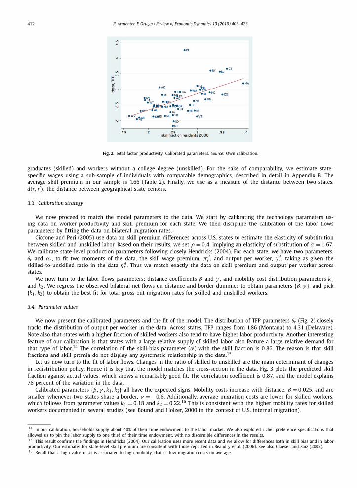
Fig. 2. Total factor productivity. Calibrated parameters. Source: Own calibration.

graduates (skilled) and workers without a college degree (unskilled). For the sake of comparability, we estimate state-specific wages using a sub-sample of individuals with comparable demographics, described in detail in Appendix B. Theaverage skill premium in our sample is 1.66 (Table 2). Finally, we use as a measure of the distance between two states,d(r, r′), the distance between geographical state centers.

3.3. Calibration strategy

We now proceed to match the model parameters to the data. We start by calibrating the technology parameters us-ing data on worker productivity and skill premium for each state. We then discipline the calibration of the labor flowsparameters by fitting the data on bilateral migration rates.

Ciccone and Peri (2005) use data on skill premium differences across U.S. states to estimate the elasticity of substitutionbetween skilled and unskilled labor. Based on their results, we set ρ = 0.4, implying an elasticity of substitution of σ = 1.67.We calibrate state-level production parameters following closely Hendricks (2004). For each state, we have two parameters,θr and αr , to fit two moments of the data, the skill wage premium, πd

r , and output per worker, ydr , taking as given the

skilled-to-unskilled ratio in the data ηdr . Thus we match exactly the data on skill premium and output per worker across

states.We now turn to the labor flows parameters: distance coefficients β and γ , and mobility cost distribution parameters k1

and k2. We regress the observed bilateral net flows on distance and border dummies to obtain parameters {β,γ }, and pick{k1,k2} to obtain the best fit for total gross out migration rates for skilled and unskilled workers.

3.4. Parameter values

We now present the calibrated parameters and the fit of the model. The distribution of TFP parameters θr (Fig. 2) closelytracks the distribution of output per worker in the data. Across states, TFP ranges from 1.86 (Montana) to 4.31 (Delaware).Note also that states with a higher fraction of skilled workers also tend to have higher labor productivity. Another interestingfeature of our calibration is that states with a large relative supply of skilled labor also feature a large relative demand forthat type of labor.14 The correlation of the skill-bias parameter (α) with the skill fraction is 0.86. The reason is that skillfractions and skill premia do not display any systematic relationship in the data.15

Let us now turn to the fit of labor flows. Changes in the ratio of skilled to unskilled are the main determinant of changesin redistribution policy. Hence it is key that the model matches the cross-section in the data. Fig. 3 plots the predicted skillfraction against actual values, which shows a remarkably good fit. The correlation coefficient is 0.87, and the model explains76 percent of the variation in the data.

Calibrated parameters {β,γ ,k1,k2} all have the expected signs. Mobility costs increase with distance, β = 0.025, and aresmaller whenever two states share a border, γ = −0.6. Additionally, average migration costs are lower for skilled workers,which follows from parameter values k1 = 0.18 and k2 = 0.22.16 This is consistent with the higher mobility rates for skilledworkers documented in several studies (see Bound and Holzer, 2000 in the context of U.S. internal migration).

14 In our calibration, households supply about 40% of their time endowment to the labor market. We also explored richer preference specifications thatallowed us to pin the labor supply to one third of their time endowment, with no discernible differences in the results.15 This result confirms the findings in Hendricks (2004). Our calibration uses more recent data and we allow for differences both in skill bias and in labor

productivity. Our estimates for state-level skill premium are consistent with those reported in Beaudry et al. (2006). See also Glaeser and Saiz (2003).16 Recall that a high value of ki is associated to high mobility, that is, low migration costs on average.


Fig. 3. Fraction of skilled workers in data (sorted by state of residence) and in the model. Note: Data from 2000 U.S. Census. 45-degree line included.

Fig. 4. Net bilateral migration flows, by skill level. Source: U.S. Census 2000, 5% sample. In total 1225 bilateral pairs, excluding two extreme observations(California–Nevada and Massachusetts–New Hampshire).

4. Model evaluation: Migration flows

We evaluate the performance of the model in accounting for data on bilateral migration flows across US states. Specif-ically, we focus on two equilibrium predictions: skilled workers migrate from one state to another if and only if unskilledworkers do so as well, and total net out-migration rates (for both types of workers) for a given state should be decreasingin the equilibrium level of utility of that state relative to the others (Proposition 4).

The first of the two predictions can be tested using the net bilateral migration matrices built with our data. Fig. 4plots the bilateral net out-migration rates of skilled and unskilled workers.17 Strikingly, the net out-migration rates for bothtypes of workers have the same sign in 83% of the cases: most pairs fall either in the top-right or bottom-left quadrants.Deviations from the pattern are not only few but also quantitatively very small. This finding is quite revealing. It shows thatthe internal migration decisions of skilled and unskilled workers are strongly aligned. This is highly informative regardingthe role of regional heterogeneity in the model. In particular, it shows that the large regional differences in TFP are whatdrives bilateral migration flows, with differences in the scarcity of skilled labor playing a much smaller role.

We now turn to the second prediction on migration flows. Namely, the negative relationship between total net out-migration rates (TNOR), for both skill types, and the state’s equilibrium utility. There is a very close relationship betweena state’s TFP level and its equilibrium level of utility thus we choose to examine total out-migration rates as a function of

17 To obtain a more informative scale in Fig. 4 we exclude two extreme observations: the bilateral flows between California and Nevada, and Massachusettsand New Hampshire. In both instances there are large flows of workers of both types in the same direction (toward Nevada and toward New Hampshire,respectively).


(a)

(b)

Fig. 5. Total net out-migration rates, by skill level and TFP: (a) unskilled workers; (b) skilled workers. Note: Total outflows minus total inflows over initialpopulation in the state. Linear fit included, not a 45-degree line. The regression has been estimated excluding four states: Connecticut, Delaware, NewJersey and New York.

the calibrated TFP parameter. Fig. 5 relates TFP levels and total net out-migration rates for unskilled and skilled workers,respectively. Two features stand out. First of all, we note the clear negative relation between TFP levels and total net out-migration rates for both skill types, as predicted by the model.18 Second, we also note that in both figures the top TFPstates display anomalous behavior (New Jersey, New York, Connecticut, Delaware).19 According to the model, these statesshould have attracted large inflows of workers. That is, they should have had very low TNOR. Instead these states lie wellabove the predicted line (based on all other states only). This anomaly is likely to reflect high housing prices and othercongestion costs. In Section 7 we present an extension of the model that includes amenities, which improves the fit of themodel.

Secondly, we note that the slope of the fitted line for TNOR as a function of TFP is substantially larger (in absolute value)for skilled workers than for unskilled. That is, as we move along the cross-section toward states with higher TFP, the modelpredicts lower outmigration rates for both workers. However, the drop is substantially larger for skilled workers. This is alsoa feature of our calibrated model, since migration costs for skilled workers are on average lower than for unskilled ones. Anobvious but important implication is that high-utility (TFP) states not only experience population inflows but, in addition,enjoy an increase in the share of skilled workers thanks to interstate migration. Conversely, low-TFP states lose populationand suffer a skill loss.

18 We can only prove this property for economies with regions with symmetric worker endowments and mobility costs. Fortunately, the differences insize and mobility in our calibrated model are not large enough to overturn Proposition 4.19 Arizona, Florida and, particularly, Nevada also appear as outliers.


Table 3Summary statistics of income redistribution at the state level in year 2000.

Mean St. dev. Min Max

Total personal current tax/state income 0.13 0.02 0.1 0.19State and local taxes plus property tax/state income 0.03 0.01 0 0.05Average income tax rate skilled family (Taxsim) 0.27 0.02 0.23 0.3Redistributive transfer (TANF + FS) $6099 $1608 $3879 $11,877

Source: For transfers, sources are U.S. Department of Health and Human Services, and the Department of Agriculture. For income tax rates, we use the NBERtax simulator (Taxsim). For aggregate tax measures, we use the BEA regional accounts 2000–2001.

Fig. 6. Total taxes over state income, data. Note: Personal current taxes at all levels plus property taxes divided by gross state product (BEA).

5. Model evaluation: Redistributive policies

The model has two key predictions regarding the cross-section of policies. First, states with a higher skill premiumshould redistribute income more aggressively. Secondly, states with higher consumption levels (say, because of relativelyhigh TFP) should provide larger transfers (in dollars). The reason is that the goal of transfers is to reduce the gap betweenthe consumption levels of skilled (rich) and unskilled (poor) workers. The goal of this section is to examine whether theserelationships are present in the data.

Building a comprehensive yet simple measure of redistribution at the state-level is not an easy task. In reality, incomeredistribution takes place both through taxes and through public spending. We focus here in measures of tax-based redis-tribution, and discuss redistribution through spending and transfers in Section 7. We also note that we did not target anyvariable related to taxes or transfers in the calibration. We shall thus evaluate the performance of the model in a qualitativefashion. It would be unreasonable to expect a tight quantitative fit between model and data along this dimension.

We choose to compare our model’s predictions to total personal taxes in the data, that is, including both federal, stateand local taxes. The main reason to include federal taxes is that in our model only equilibrium allocations are determined. Inthese allocations, the difference between, say, income and consumption is total net taxes (state and federal).20 Implicitly, weare assuming that the federal government sets taxes and transfers first. Then each state’s fiscal authority decides whetherto increase or decrease the amount of redistribution taking place within its borders.21

Let us start by comparing model and data regarding the size of total taxes relative to state income. The Bureau ofEconomic Analysis reports tax revenue by state annually. As summarized in Table 3, on average, total personal taxes (mainly,state plus federal income tax) in 2000 were 13.26% of state income. Differences across states are quite large, ranging from9.84% to 19.23%.22 In addition, Fig. 6 shows that there is a strong positive relationship between a state’s skill fraction andtotal personal taxes as a fraction of state income. We can now compute the analog measure in our calibrated economy. Thedistribution of tax revenue over state income predicted by the model turns out to be quite similar to the one in the data,with a mean of 11.03% and ranging from 7.22% to 16.14%. The model also generates the positive relationship found in thedata.

Next, we introduce a more direct measure of tax-based redistribution for which the model has a clear testable im-plication. A central prediction of the model is that states with a higher skill premium should redistribute income more

20 Local taxes can be safely ignored because they tend to be low with little progressivity. Thus their redistribution effects are negligible.21 The working paper version reports alternative measures excluding federal taxes; the results presented were not sensitive to the change in measures.22 Alaska, Florida, Nevada, South Dakota, Texas, Washington, and Wyoming have no state income tax. In addition, New Hampshire and Tennessee only tax

capital income.


Fig. 7. Comprehensive measure of tax-based redistribution (progressivity) and skill premium. Note: Progressivity measure uses income and property taxescombined. Data from BEA and U.S. Census. We include the best linear fit.

aggressively. In terms of taxation, this means that their tax schedules should be more progressive. In the model, redistribu-tion can be easily measured by the gap between skilled workers’ pre-tax income and their consumption. However, in thedata, individual after-tax income and consumption do not coincide (because of savings). As a result, it is more appropriateto measure tax-based redistribution by comparing incomes before and after taxes. Moreover, in reality, even relatively poorhouseholds pay taxes. Therefore the redistributive content of taxes depends on their progressivity. Keeping these points inmind, we introduce the following measures of income redistribution through taxation. The bulk of tax revenue at the statelevel comes from income taxes, property taxes, and sales taxes. The latter is close to a linear tax and, hence, displays little orno progressivity. Thus, our measure of tax-based redistribution is the sum of the progressivity of the income and propertytaxes.

To build our measure of progressivity of the tax system, we proceed in four steps. First, we use a 1% sample of theU.S. Census (with homogeneous age, gender, and race) to estimate state-level individual income, home values, and propertytaxes, by education level. Secondly, we use the NBER’s income tax simulator (Taxsim) to compute the income tax (state plusfederal) that the average skilled/unskilled worker in each state would have had to pay in year 2000.23 Third, we measureincome tax progressivity as the difference between the average income tax rate paid by the (average) skilled worker minusthe average income tax rate paid by the (average) unskilled worker. The average income tax rate of an individual is definedas the ratio of the income tax computed using the tax simulator to that individual’s total income. Fourth, we measureproperty tax progressivity by computing the ratio of property tax (in dollars) over the total income for that worker andthen take the difference across skill types.

Fig. 7 reports the sum of the two measures of progressivity against the college wage premium in each state. We finda strong, positive relationship between the two variables. The OLS estimated slope is 0.079 (with standard error 0.011). Inwords, states with a higher skill premium choose more progressive tax schedules. A closer look at the data reveals that thepositive association is driven by the progressivity of the income tax. This is because in most states total income taxes aremuch higher than property taxes.24

6. The effect of worker mobility on redistribution policies

Finally we turn to the main goal of this paper. We ask how worker mobility across U.S. states has affected state-levelredistribution policies. In particular, we would like to know whether labor mobility has impaired income redistribution or,more generally, whether it is a force of convergence or divergence in policies. We focus on two dimensions of redistribution:the average tax rate borne by skilled workers and the size of the transfer received by each unskilled worker.

The exercise we perform is the following. We compare the cross-sections of policies in equilibrium and in a coun-terfactual scenario where migration costs are prohibitively high and no worker finds it profitable to migrate. Equilibriumallocations can be computed in a straightforward manner for both scenarios. In the autarky (no-mobility) scenario, we com-pute the allocation taking the distribution of workers by state of birth from the data. We keep the technology parametersconstant across the two scenarios.

23 We consider actual differences in the taxation of labor (wage) income and capital income. We also deduct the property tax. Thus, differences acrossstates in the income tax of the average skilled worker reflect both differences in tax rates and in factor prices across states.24 On average, across all states, skilled (unskilled) workers pay $9600 ($3700) in income tax and only $1425 ($846) in property tax.


(a)

(b)

Fig. 8. Policy convergence due to labor mobility. Model without amenities. (a) Tax rates: autarky versus equilibrium. (b) Transfers: autarky versus equilib-rium. Notes: (a) Autarky means that we use data on individuals sorted by state of birth. A linear regression has intercept 0.06 (0.01) and slope 0.75 (0.05)with standard errors in parentheses. R-squared is 0.82 and correlation coefficient 0.90. 45-degree line included. (b) A linear regression has intercept 0.006(0.001) and slope 0.93 (0.01) with standard errors in parentheses. R-squared is 0.99 and correlation coefficient 0.99. 45-degree line included.

6.1. Tax rates

Our first important result is that worker mobility has induced convergence in tax rates. Fig. 8(a) reports income tax ratesunder autarky (horizontal axis) and in equilibrium (vertical axis). If all points lined up in a horizontal line, we would havefull convergence. If they lied on the 45 degree line then there would be a complete absence of convergence. A simple wayto measure the degree of policy convergence is by estimating the slope of a linear regression (with an intercept), wherethe dependent variable is the tax rate in equilibrium and the explanatory variable is the tax rate in autarky. If the slopecoefficient is one then we shall say that there is no policy convergence at all. If the slope coefficient is zero we shall saythat there is complete convergence.

The points on the scatter plot reveal some convergence in tax rates (slope 0.75) as a result of interstate worker migration.The states with the highest autarky tax rates have experienced a reduction in tax rates as a result of migration, for instance,Virginia (VA) and Georgia (GA). The converse is true for most states with the lowest autarky tax rates, such as North Dakota(ND) and West Virginia (WV). It is also worth noting that we do not find downward pressure on tax rates: the averagetax rate is roughly constant around 23 percent in the two scenarios (Table 4). This finding suggests that the often-voicedconcerns that worker mobility triggers a “race to the bottom” in income redistribution policies seem misplaced.

These changes in policies are the result of changes in skill composition driven by migration. Some states (e.g. VA andGA), experienced a large inflow of workers from other states, which led to a reduction in skill premia and in redistributivetaxes. Recall that high-TFP states attracted both types of workers, skilled and unskilled. For VA and GA, the inflow of bothworker types induced an increase in the skilled–unskilled ratio: skilled workers make up a larger fraction of in-migrantsthan in the original population of the state. Both GA and VA have initial skill ratios below the national average, so migrationflows bring some reversion to the mean. Moreover, skilled workers are more mobile, so they are over-represented among


Table 4Equilibrium versus autarky. Cross-sections of redistributive policies.

Mean St. dev. Min Max

EquilibriumTax rate on skilled workers 0.23 0.04 0.12 0.30Transfer per recipient $6964 $2422 $3105 $12,208

AutarkyTax rate on skilled workers 0.23 0.05 0.13 0.32Transfer per recipient $6868 $2577 $2594 $12,398

Table 5Equilibrium versus autarky.

Winner statesa Loser statesb

Change in tax rate −0.02 0.05Perc. change in transfers −0.03 0.155Skill gain 0.015 −0.033TFP 3.16 2.12

a Winner states are the 5 states with the largest skill gain (AZ, DE, VA, WA, GA) according to the model.b Loser states are the 5 with the largest skill drain (ND, MS, LA, SD, WV).

migrants. In contrast, states like ND and WV suffered skill-biased outflows that raised the relative price of skilled labor andthe need for redistributive taxation.

Let us now quantify these changes. It is helpful to sort states from lower to higher skill gain, defined as the fraction ofskilled workers in the mobility equilibrium minus the fraction in autarky. Let us now focus on the top and bottom 5 statesby skill gain.25 Skill-winners have an average TFP that is 20 percent above the mean, while skill-losers’ TFP is 19 percentbelow the mean.

As displayed in Table 5, the average skill-winning state experienced an increase in the fraction of skilled workers of1.5 percentage points. This led to a reduction of 2 percentage points in the average tax rate. Conversely, on average, skill-losing states suffered a reduction in the share of skilled workers equal to 3.3 percentage points, causing the tax rate toincrease by 5 percentage points on average.

6.2. The size of transfers

Let us now turn to the effect of worker mobility on the cross-section of redistributive transfers. The results are displayedin Fig. 8(b), which reports equilibrium transfers in the two scenarios. The main finding is that there is some convergence butto a much more limited extent that in tax rates. In terms of the analogous convergence regression, the slope now is 0.93,rather close to one (no convergence). The relative insensitivity of transfers per recipient is due to an offsetting tax-baseeffect. The budget constraint of the regional government implies that for a given income tax τ , the transfer handed out tothe unskilled in the region has to be τη, that is, the product of the tax on skilled workers times the skilled-to-unskilledratio in the population. As a result, states experiencing an increase in η will have both a larger tax base and a lower skillpremium. The resulting lower wage inequality leads to a lower redistributive tax. The size of the transfer, τη, will fall by lessthan the tax and might even increase. The net effect depends on parameter values. In our calibration, the two effects almostbalance out. In response to an increase in skill fraction, the fiscal authority chooses to keep the size of the transfer relativelyunchanged, while vigorously reducing the tax on skilled workers.26 Table 5 reports the percentage change in the size oftransfers (per recipient) in skill-winning and in skill-losing states. While the former reduced their transfers by 3 percent onaverage, the latter increased them by 15.5 percent.

7. Robustness

7.1. Model with amenities

As we noted earlier, the calibrated model fails to account for the high out-migration rates from the states with thehighest levels of TFP. This section extends the model by introducing exogenous region-specific factors that influence thelocation decisions of both types of workers but are not related to income. We refer to these factors as amenities. Weatherconditions are a good example of a possible determinant of migration decisions which is not directly related to wages.

25 The top 5 skill-winning states in the data were Arizona, Georgia, Maryland, Virginia and Colorado and the 5 suffering the largest skill drain were NorthDakota, Wyoming, Iowa, South Dakota, and Wisconsin. According to our model the top states are Arizona, Delaware, Virginia, Washington and Georgia andthe bottom ones are North Dakota, Mississippi, Iowa, South Dakota and West Virginia.26 Recall that TFP differences also affect the size of transfers.


We introduce amenities as follows. Total welfare for a worker of type i in region r is given now by

U(xr

i

) + Ar

where Ar is the utility flow of the amenities in region r. Separability implies that, given a skill ratio, the second best allo-cation with amenities coincides with the allocation in the baseline model. Thus amenities are simply additional parametersthat improve the fit of the model, but do not affect the mechanics of income redistribution.

We have to update the equilibrium condition for the mobility decisions. Now a national equilibrium requires that foreach r � R , all individually profitable moves from r to r′ have taken place. If δi(r, r′) < (R − 1)−1, we have that

U(xr′

i

) + Ar′ − U(xr

i

) − Ar � μi(r, r′),

with equality if δi(r, r′) > 0, for all r′ �= r and i = 1,2. If δi(r, r′) = (R − 1)−1 then

U(xr′

i

) + Ar′ − U(xr

i

) − Ar � μi(r, r′).

With the additional degrees of freedom granted by the vector of amenities parameters, {Ar}, we can improve the fitof migration flows. The correlation between observed and predicted skill ratios is 0.96 and the model explains close to90 percent of the variation in the data, compared to 0.87 and 0.76 in the model without amenities. The amenities do notoverthrow completely the welfare ranking given by TFP levels.27 However, the calibration assigns low amenities to the stateswith highest TFP in order to explain their relatively high out-migration rates.

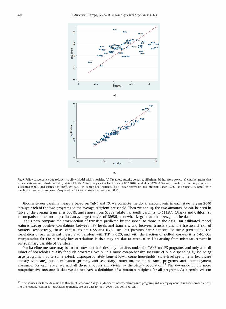
We now re-evaluate the impact of labor mobility in policies using the model with amenities. Figs. 9(a) and 9(b) comparetax rates and transfers, respectively, in autarky and in equilibrium. We largely confirm our findings from the previous sec-tion: significant convergence in tax rates and, to a lesser degree, in the size of transfers. In fact, the extended model displaysa larger degree of policy convergence, both in tax rates and in transfers. In terms of the policy convergence regressions in-troduced early, the corresponding slopes are 0.26 and 0.90 (for tax rates and transfers, respectively), compared to 0.75 and0.93 in the model without amenities.28 We also note that the changes in the share of skilled workers in skill-winning andskill-losing states is much larger than in the model without amenities, respectively, 5.7 and −4.7 on average. This accountsfor the larger changes in redistributive policies before and after migration.

An alternative, more sophisticated approach would be to introduce immobile factors (e.g. land) as in Roback (1982).Differences in TFP across locations would then be offset by higher land prices. This mechanism could explain the observedout-migration in the states with the highest TFP. However, introducing immobile factors greatly complicates the analysis inthe presence of mobility frictions and endogenous policies.

7.2. Alternative definitions of migration

We now experiment with two alternative empirical definitions of a migrant, in addition to our baseline (Definition I).Specifically, Definition II restricts the sample to individuals born between 1970 and 1975. Definition III maintains the birthcohorts of the baseline sample (1955–1975) but focuses on migration events that took place between 1995 and 2000 (seeAppendix B.1 for details). We examine whether the cross-sections of the share of skilled workers are sensitive to the specificempirical definition of migrant that we use. Recall that changes in the share of skilled workers in a state are the main driverof changes in redistribution policy.

We find very small changes in the cross-sectional distribution of skilled workers across states after migration accordingto each migrant definition. Under Definition II the skill ratio tends to be slightly below the skill ratio under the baselinedefinition, due to the lower overall average age. There are no significant changes when using Definition III either. Laborflows for both types of workers are highly correlated across definitions. We thus conclude that the skill composition ofmigrants and residents is robust to alternative definitions.

7.3. Redistribution via transfers

We now discuss measures of redistribution through transfers. Following Meyer (2000), we focus on data for the two mainincome-maintenance programs: Temporary Aid to Needy Families (TANF) and Food Stamps (FS). States enjoy a high degree ofdiscretion in deciding the size of these transfers. The U.S. Department of Health and Human Services, and the Department ofAgriculture, respectively, supply data on spending per recipient by state on these programs. With this measure we are takinga quite narrow view on transfers. The reason is that we want to be sure that we are obtaining a measure of redistribution.These programs are means-tested and, therefore, we are confident that higher spending in these programs unambiguouslycorresponds to greater redistribution. The trade-off is that we are leaving out several types of expenditure that are alsopartially redistributing income, and that recipients of the TANF and FS are not a representative sample of unskilled workersin our model. Below we build a broader measure of redistributive spending that includes public healthcare and education.

27 The working paper version contains details in the calibration and resulting parameter values for the model with amenities.28 These results are virtually unchanged if we use the actual skill ratios in the data rather than the predicted skill ratios.


(a)

(b)

Fig. 9. Policy convergence due to labor mobility. Model with amenities. (a) Tax rates: autarky versus equilibrium. (b) Transfers. Notes: (a) Autarky means thatwe use data on individuals sorted by state of birth. A linear regression has intercept 0.17 (0.02) and slope 0.26 (0.08) with standard errors in parentheses.R-squared is 0.19 and correlation coefficient 0.43. 45-degree line included. (b) A linear regression has intercept 0.009 (0.002) and slope 0.90 (0.03) withstandard errors in parentheses. R-squared is 0.95 and correlation coefficient 0.97.

Sticking to our baseline measure based on TANF and FS, we compute the dollar amount paid in each state in year 2000through each of the two programs to the average recipient household. Then we add up the two amounts. As can be seen inTable 3, the average transfer is $6099, and ranges from $3879 (Alabama, South Carolina) to $11,877 (Alaska and California).In comparison, the model predicts an average transfer of $8686, somewhat larger than the average in the data.

Let us now compare the cross-section of transfers predicted by the model to those in the data. Our calibrated modelfeatures strong positive correlations between TFP levels and transfers, and between transfers and the fraction of skilledworkers. Respectively, these correlations are 0.88 and 0.73. The data provides some support for these predictions. Thecorrelation of our empirical measure of transfers with TFP is 0.23, and with the fraction of skilled workers it is 0.40. Ourinterpretation for the relatively low correlations is that they are due to attenuation bias arising from mismeasurement inour summary variable of transfers.

Our baseline measure may be too narrow as it includes only transfers under the TANF and FS programs, and only a smallsubset of households qualify for such programs. We build a more comprehensive measure of public spending by includinglarge programs that, to some extent, disproportionately benefit low-income households: state-level spending in healthcare(mostly Medicare), public education (primary and secondary), other income-maintenance programs, and unemploymentinsurance. For each state, we add all these amounts and divide by the state’s population.29 The downside of the morecomprehensive measure is that we do not have a definition of a common recipient for all programs. As a result, we can

29 The sources for these data are the Bureau of Economic Analysis (Medicare, income-maintenance programs and unemployment insurance compensation),and the National Center for Education Spending. We use data for year 2000 from both sources.


only report data per capita and not per recipient. Moreover, skilled households are likely to benefit significantly from someof these programs as well. Thus only a fraction of this spending is truly redistributive.

Transfers under TANF and FS were $6099 per recipient. In per-capita terms (that is, dividing total spending in TANF andFood Stamps over state population), the average value of TANF and FS is very low, $243. Obviously, our more comprehensivemeasure leads to a much higher average amount, equal to $3622 per capita. Education accounts for almost two thirds ofthis value, with healthcare being responsible for most of the remaining amount.

We now examine the relationship between our more comprehensive measure of transfers, TFP and the share of skilledworkers. Specifically, we estimate two simple linear regression models where the dependent variable is the amount ofspending per capita in each state and the explanatory variable is, in one case, our calibrated measure of TFP, and in theother, the share of skilled in the state. In both cases the slope coefficient is positive and highly significant.30

In conclusion, the predictions of the model are in line with the main qualitative features of the cross-section data onincome redistribution, both when redistribution takes place through taxes and through spending.

8. Conclusions

Our main goal was to study the effect of worker mobility on redistributive policies in U.S. states. Our main finding is thatworker mobility has induced substantial convergence, but no downward pressure, in tax rates. We also find some evidenceof migration-induced convergence in transfer levels, but to a much lesser degree due to an offsetting tax-base effect.

Our analysis makes clear that differences in TFP are the key determinant of income, labor flows, and transfers per recip-ient. This is very much in line with recent findings in the international migration literature—see for example Rosenzweig(2007), Grogger and Hanson (2008), and Ortega and Peri (2009).

We hope the model presented here can be the basis for further quantitative work on the study of regional tax compe-tition in a context of realistic labor mobility. Our model has made a number of assumptions, which should be relaxed infuture work. In particular, it would be interesting to incorporate immobile factors, such as land, to explore the dynamics ofthe model, and to endogenize the link between skills and TFP.

Appendix A. Proofs

Proof of Proposition 1. It is straightforward to show that a competitive equilibrium allocation given τ is pinned down by

MRS(c1, l1) = F1(l1, ηl2),

MRS(c2, l2) = F2(l1, ηl2),

c1 + ηc2 = F (l1, ηl2),

c2 = F2(l2, ηl2)l2 − τ .

It is clear that the skilled (unskilled) welfare is decreasing (increasing) with τ . Hence there is a value of τ such that theincentive compatibility constraint (IC) binds. The resulting competitive equilibrium allocations are second-best. �Proof of Proposition 2. Necessary first order conditions from (2) are then

u′(c1) = u′(c2),

MRSi(ci, li) = Fi(l1, ηl2) for i = 1,2,

where MRSi = v ′(li)/u′(ci). Hence c1 = c2. If l2 > l1, the incentive compatibility constraint (IC) would be violated. If l1 � l2,then

F1

(1,

ηl2l1

)< F2

(1,

ηl2l1

)

as skilled labor is the scarce factor. First order conditions imply then v ′(l1) < v ′(l2) but this contradicts l1 � l2. This provesproperty 1.

For property 2, assume that second-best allocation x has

F1

(1, η

l2l1

)� F2

(1, η

l2l1

).

The properties of F and η < η, imply l2 > l1. The incentive compatibility constraint implies then that c2 > c1. Strict concavityof U implies that if c2 > c1, l2 > l1, then − Ul(c2,l2)

Uc(c2,l2)> − Ul(c1,l1)

Uc(c1,l1). But then x is incompatible with the necessary first order

conditions of problem (2) since MRS2 > MRS1 implies that F2 > F1, contradicting our initial hypothesis.

30 The output of these regressions and two supporting figures are available upon request.


Now we prove the third property. By first order conditions for second-best allocation, MRS(c2, l2) > MRS(c1, l1). SinceU (c1, l1) = U (c2, l2) and indifference curves are strictly convex, we have that (c2, l2) � (c1, l1).

Property 4 also follows. Assume τ � 0. Because skilled workers are scarce, they will be strictly better off, contradictingproperty 1. �Proof of Proposition 3. We first prove that for any η < η, second-best allocations x satisfy c2 < F2(l1, ηl2)l2. Considerthe set A = {(c, l): c � F2(l1, ηl2)(l − l2) + c2}. Since MRS(c2, l2) = F2(l1, ηl2) and preferences are strictly concave, for any(c, l) ∈ A, U (c, l) � U (c2, l2), with equality sign iff c = c2 and l = l2. Therefore (c1, l1) /∈ A since the incentive compatibilityconstraint is binding and l1 �= l2 as Proposition 2 indicates. This implies

c1 > c2 + F2(l1, ηl2)(l1 − l2)

and since F1(l1, ηl2) < F2(l1, ηl2),

c1 − F1(l1, ηl2)l1 > c2 − F2(l1, ηl2)l2.

Using constant returns to scale, the resource constraint can be written as(c1 − F1(l1, ηl2)l1

) + η(c2 − F2(l1, ηl2)l2

) = 0

therefore c2 < F2(l1, ηl2)l2.We next show that second-best allocation x is feasible at η′ . Note that

F(l1, η

′l2) − F (l1, ηl2) = F2(l1, ηl2)l2

(η′ − η

),

where η ∈ [η,η′] by the Taylor theorem. Using the concavity of F ,

F(l1, η

′l2) − F (l1, ηl2) > F2

(l1, η

′l2)l2

(η′ − η

).

Since the resource constraint is binding we have

F(l1, η

′l2) − c1 − η′c2 >

(F2

(l1, η

′l2)l2 − c2

)(η′ − η

).

Since we proved that F2(l1, η′l2)l2 − c2 > 0, allocation x satisfies the resource constraint with strict inequality sign whenη′ > η.

By continuity, there exists c2 > c2 such that F (l1, η′l2) > c1 + η′c2. It is clear then that x = {c1, c2, l1, l2} is feasible andincentive compatible with U (c1, l1)+ηU (c2, l2) < U (c1, l1)+ηU (c2, l2). Since allocations x′ cannot do worse than x, and theincentive constraint is binding for η′ , the result follows. �Appendix B. Data

B.1. U.S. Census 2000

Our data is a 5% public-use sample of the 2000 U.S. Census extracted using IPUMS. We define an individual as skilled ifhe had a college degree and unskilled otherwise. We build three alternative definitions of internal migrant.

Definition I (Baseline). Consider the sample of individuals born in the United States between 1955 and 1975 (age 25–45in year 2000). Define a migrant as an individual whose state of residence in 2000 differed from his state of birth. Webuild the labor endowments in each state by sorting individuals according to their state of birth. Likewise, we build theafter-migration worker distribution by sorting individuals by their residence in year 2000.

Definition II. We consider a more homogeneous sample in terms of year of birth, namely, individuals born between 1965and 1970 (age 30–35 in year 2000). As in the baseline case, we define a migrant as an individual whose state of birth differsfrom his state of residence in year 2000. Note that state of birth now coincides with state of residence around 1967.

Definition III. We now employ a definition that exactly determines the year of migration. As in the baseline case, weconsider individuals born between 1955 and 1975 (age 25–45 in year 2000). But now we define a migrant as an individualwhose state of residence in 1995 differs from his/her state of residence in year 2000.

Skill premia (skilled-to-unskilled ratios of hourly wages) are also obtained from the sample Census sample. To enhancecomparability of skill premia across states, we estimate state-level hourly wages restricting to a highly homogeneous sub-sample. In particular, we restrict to white males, age 25–45, that are part of the workforce.

B.2. Bureau of Economic Analysis, Regional Accounts

We compute output per worker by dividing state personal income in year 2001 by total employment in the state inthe same year. Our data on tax revenue is also from the BEA. We average over the period 2000–2002. Our main aggregatemeasure of taxes is personal current taxes (federal, state, and local) over state income. This is mainly the income tax.


B.3. NBER’s Taxsim

To compute average income tax rates, for skilled workers, we use NBER’s income tax simulator (Taxsim) to compute thetax that a typical skilled family would have to pay in each of the U.S. states, keeping family income constant. We thencompute the average tax income tax rate of a skilled worker dividing by pre-tax income. In particular, we assume that atypical family is a two-person household with a joint income of $200,000. The exact figure does not matter much, only thefact that it is kept constant across all states. Leigh (2005) also uses Taxsim in an interesting application.

B.4. U.S. Department of Health and Human Services

Following Meyer (2000), we consider two types of redistributive transfers: Temporary Aid to Needy Families (TANF) andFood Stamps (FS). States have had considerable autonomy in deciding the size of TANF and FS transfers particularly since1996 when Aid for Families with Dependent Children (AFDC) was replaced by TANF. Using data from the U.S. Departmentof Health and Human Services, we define each state’s transfer as the sum of TANF (and similar state programs) and FoodStamps for a family of 3 with no income in each state in year 2000. The average transfer across all states was 6101 U.S.Dper household. The same family would have received 3879 U.S.D in Alabama, the state with the lowest transfers. At theother end of the spectrum, this family would have received 11,877 U.S.D in Alaska or 10,278 U.S.D in California, the stateswith the highest transfers.

References

Aghion, P., Boustan, L., Hoxby, C., Vandenbussche, J., 2005. Exploiting states’ mistakes to identify the causal impact of higher education on growth. Mimeo.Albouy, D., 2009. The unequal geographic burden of federal taxation. Journal of Political Economy 117 (4), 635–667.Armenter, R., Ortega, F., 2009. Credible redistribution policy and skilled migration. Universitat Pompeu Fabra. Mimeo.Beaudry, P., Doms, M., Lewis, E., 2006. Endogenous skill bias in technology adoption: city-level evidence from the IT revolution. NBER working paper 12521.Bewley, T., 1981. A critique of Tiebout’s theory of local public expenditures. Econometrica 49, 713–740.Blanchard, O., Katz, L., 1992. Regional evolutions. Brooking Papers on Economic Activity 23, 1–75.Bound, J., Holzer, H.J., 2000. Demand shifts, population adjustments, and labor market outcomes during the 1980s. Journal of Labor Economics 18 (1),

20–54.Ciccone, A., Peri, G., 2005. Long-run substitutability between more and less educated workers: Evidence from U.S. states, 1950–1990. The Review of Eco-

nomics and Statistics 87 (4), 652–663.Coen-Pirani, D., 2006. Understanding gross workers flows across U.S. states. Tepper School of Business. Mimeo.Cremer, H., Pestieau, P., 1998. Social insurance, majority voting, and labor mobility. Journal of Public Economics 68 (3), 397–420.Dahl, G., 2002. Mobility and the return to education: Testing a Roy model with multiple markets. Econometrica 70 (6), 2367–2420.Epple, D., Romer, T., 1991. Mobility and redistribution. Journal of Political Economy 99 (4), 828–858.Glaeser, E., Saiz, A., 2003. The rise of the skilled city. NBER working paper 10191.Greenstone, M., Hornbeck, R., Moretti, E., 2008. Identifying agglomeration spillovers: Evidence from million dollar plants. NBER working paper 13833.Greenwood, M.J., 1969. An analysis of the determinants of geographic labor mobility in the United States. Review of Economics and Statistics 51, 189–194.Grogger, J., Hanson, G.H., 2008. Income maximization and the selection and sorting of international migrants. NBER working paper 13821.Hassler, J., Rodriguez-Mora, J.V., Storesletten, K., Zilibotti, F., 2005. A positive theory of geographic mobility and social insurance. International Economic

Review 46, 263–303.Hendricks, L., 2004. Why does educational attainment differ across U.S. states? Iowa State University. Mimeo.Kennan, J., Walker, J., 2006. The effect of expected income on individual migration decisions. Working paper, University of Wisconsin–Madison.Leigh, A., 2005. Can redistributive state taxes reduce inequality? Australian National University Centre for Economic Policy Research discussion paper 490.Lkhagvasuren, D., 2005. Large locational differences in unemployment despite high labor mobility. Mimeo.Meyer, B., 2000. Do the poor move to receive higher welfare benefits? Mimeo.Mirrlees, J., 1971. An exploration in the theory of optimal income taxation. The Review of Economic Studies 38 (2), 175–208.Morelli, M., Yang, H., Ye, L., 2008. Competitive nonlinear taxation and constitutional choice. Mimeo.Moretti, E., 2004. Workers’ education, spillovers and productivity: Evidence from plant-level production functions. American Economic Review 94, 656–690.Oates, W.E., 1972. Fiscal Federalism. Harcourt Brace Jovanovich, New York.Ortega, F., Peri, G., 2009. The causes and effects of international migrations: Evidence from OECD countries 1980–2005. NBER working paper 14833.Roback, Jennifer, 1982. Wages, rents, and the quality of life. Journal of Political Economy 90, 1257–1278.Rosen, Sherwin, 1979. Wage-based indexes of urban quality of life. In: Mieszkowski, P., Strasz-heim, M. (Eds.), Current Issues in Urban Economics. Johns

Hopkins Univ. Press, Baltimore.Rosenzweig, Mark, 2007. Education and migration: A global perspective. Yale. Mimeo.Schmidheiny, K., 2005. Income segregation and local progressive taxation: Empirical evidence from Switzerland. Journal of Public Economics 90 (3), 429–

458.Tiebout, C., 1956. A pure theory of local expenditures. Journal of Political Economy 64 (5), 416–424.Wilson, J., Wildasin, D., 2004. Capital tax competition: Bane or Boom? Journal of Public Economics 88 (6), 1065–1091.Zodrow, G., Mieszkowski, P., 1986. Pigou, Tiebout, property taxation, and the underprovision of local public goods. Journal of Urban Economics 19 (3),

356–370.

Documents

Credible redistributive policies and migration across U.S ...qcpages.qc.cuny.edu/~fortega/research/armenter_ortega_red2010.pdf · 404 R. Armenter, F. Ortega / Review of Economic Dynamics