Credal Networks for Military IdentificationProblems⋆

aIDSIA, Galleria 2, CH-6928 Manno (Lugano), SwitzerlandbArmasuisse (W+T), Feuerwerkerstrasse 39, CH-3600 Thun, Switzerland

Alessandro Antonuccia, Ralph Bruhlmannb , Alberto Piattia,∗,Marco Zaffalona

Abstract

Credal networks are imprecise probabilistic graphical models generalizing Bayesian net-works to convex sets of probability mass functions. This makes credal networks particu-larly suited to model expert knowledge under very general conditions, including states ofqualitative and incomplete knowledge. In this paper, we present a credal network for riskevaluation in case of intrusion of civil aircrafts into a restricted flight area. The differentfactors relevant for this evaluation, together with an independence structure over them, areinitially identified. These factors are observed by sensors, whose reliabilities can be af-fected by variable external factors, and even by the behaviour of the intruder. A model ofthese observation processes, and the necessary fusion scheme for the information returnedby the sensors measuring the same factor, are both completely embedded into the structureof the credal network. A pool of experts, facilitated in their task by specific techniques toconvert qualitative judgements into imprecise probabilistic assessments, has made possi-ble the quantification of the network. We show the capabilities of the proposed model bymeans of some preliminary tests referred to simulated scenarios. Overall, we can regardthis application as a useful tool to support military experts in their decision, but also as aquite general imprecise-probability paradigm for information fusion.

Keywords: Credal Networks, Information Fusion, Sensor Management, Tracking Sys-tems.

⋆ This research was supported by Armasuisse, and partially bythe Swiss NSF grantsn. 200020-116674/1 and n. 200020-121785/1.∗ Corresponding author.

Email addresses:alessandro@idsia.ch (Alessandro Antonucci),ralph.bruehlmann@ar.admin.ch (Ralph Bruhlmann),alberto.piatti@idsia.ch (Alberto Piatti),zaffalon@idsia.ch (MarcoZaffalon).

Preprint submitted to Elsevier Science March 2, 2009

1 Introduction

In the recent times, the establishment of a restricted or prohibited flight area aroundimportant potential targets surveyed by the Armed Forces has become usual prac-tice, also in neutral states like Switzerland, because of the potential danger of terrorthreats coming from the sky. A prohibited flight area is an airspace of definite di-mensions within which the flight of aircrafts is prohibited.A restricted flight areais an airspace of definite dimensions within which the flight of aircrafts is restrictedin accordance with certain specified conditions [17].

Once a restricted flight area is established for the protection of a single strategicobject, all the aircrafts flying in this region without the required permissions areconsideredintruders. The restricted flight area can be imagined as divided in twoconcentric regions: an external area, devoted to the identification of the intruder,where the intruder is observed by many sensors of the civil and military Air TrafficControl and by the interceptors, and an internal area, whichis a small region con-taining the object to protect and the military units, where fire is eventually releasedif the intruder is presumed to have bad aims.

Clearly, not all the intruders have the same intentions: there are intruders with badaims, calledrenegades, intruders with provocative aims, erroneous intruders, andeven aircrafts that are incurring an emergency situation. Since only renegades rep-resent a danger for the protected object, the recognition ofthe intruder’s aim plays acrucial role in the following decision. This is the identification problem we addressin this paper.

The problem is complex for many reasons: (i) the risk evaluation usually relies onqualitative expert judgements; (ii) it requires the fusionof information coming fromdifferent sensors, and this information can be incomplete or partially contradictory;(iii) different sensors can have different levels of reliability, and the reliability ofeach sensor can be affected by exogenous factors, as geographical and meteoro-logical conditions, and also by the behaviour of the intruder. A short review of theproblem and some details about these difficulties are reported in Sect. 2.

In this paper, we proposecredal networks[7] (Sect. 3) as a mathematical paradigmfor the modeling of military identification problems. Credal networks are impre-cise probabilistic graphical models representing expert knowledge by means ofsets of probability mass functions associated to the nodes of a directed acyclicgraph. These models are particularly suited for modeling and doing inference withqualitative, incomplete, and also conflicting information. All these features appearparticularly important for the military problem under consideration.

More specifically, we have developed a credal network that evaluates the level ofrisk associated to an intrusion. This is achieved by a numberof sequential steps:determination of the factors relevant for the risk evaluation and identification of

2

a dependency structure between them (Sect. 4.1); quantification of this qualita-tive structure by imprecise probabilistic assessments (Sect. 5.1); determination ofa qualitative model of the observation process associated to each sensor, togetherwith the necessaryfusion schemeof the information collected by the different sen-sors (Sect. 4.2); quantification of this model by probability intervals (Sect. 5.2). Ananalysis of the main features of our imprecise-probabilityapproach to informationfusion is indeed reported in Sect. 6.

The credal network is finally employed to evaluate the level of risk, which is simplythe probability of the risk factor conditional on the information collected by thesensors in the considered scenario. A description of the procedure used to updatethe network, together with the results of some simulations,is reported in Sect. 7.

Summarizing, we can regard this model as a practical tool to support military ex-perts in their decisions for this particular problem.1 But, at the same time, ourcredal network can be regarded as a prototypical modeling framework for generalidentification problems requiring information fusion.

2 Military Aspects

This section focuses on the main military aspects of the identification problem ad-dressed by this paper. Let us first report the four possible values of the RISK FAC-TOR 2 by which we model the possible intentions of the intruder.

(i) Renegade. The intruder intends to use his aircraft as a weapon to damagethe strategic target defended by the restricted flight area.3

(ii) Agent provocateur. The aim is to provoke or demonstrate. The intruderknows exactly what he is doing and does not want to die, therefore he isexpected to react positively to radio communication at a certain moment.

(iii) Erroneous. The intruder is entering the restricted flight area becauseofan error in the flight path due to bad preparation of the flight or insufficienttraining level.

(iv) Damaged. This is an intruder without bad aims that is incurring an emer-gency situation due to a technical problem. The pilot does not necessarily

1 The support we provide is represented by the probabilistic information about the actuallevel of risk associated to an intrusion. Decisions about possible interventions can be basedon this information, but are still taken by military experts. A model of such decision process,to be embedded into the network structure, could be explored(e.g., by considering the ideasin [1] and their development in [10]), but is beyond the scopeof this paper.2 The following typographical convention is used: the variables considered in our proba-bilistic model are written in SMALL CAPITALS and their possible states intypewriter.3 There are also some subcategories of terrorists (e.g., poison sprayers), which will beconsidered only in a future work.

3

knows what he is doing because of a possible situation of panic. A damagedintruder can react negatively to radio communications, as their instrumentscould be switched off because of electrical failures. A proper identification ofdamaged intruders is very important because they can be easily confused withrenegades.

In order to decide which one among these four categories reflects the real aim ofthe intruder an appropriate identification architecture should be set up. Fig. 1 dis-plays the structure typically employed in Switzerland. When a restricted flight areais set up for the protection of an important object, theAir Defence Direction Center(ADDC) is in charge of the identification of possible intruders. The ADDC collectsthe information provided by three main sources: (i) the sensors of the civilAir Traf-fic Control (ATC), (ii) the sensors of the military ATC, (iii) the interceptors of theSwiss Air Force devoted to Air Police missions. Once this evidential informationhas been collected, the ADDC performs the identification of the aim of the intruder.

No

n-c

oo

per

ativ

e

iden

tifica

tion

Co

op

erat

ive

iden

tifica

tion

Iden

tif.b

y

inte

rven

tion

Iden

tifica

tion

by

tech

nic

alin

stru

men

ts

CIVIL ATCSSRs and radio communications

MILITARY ATCPrimary radars ADDC

AIR POLICEInterception

Figure 1. The identification architecture.

The civil ATC sensors are based on a collaborative communication between theATC and the intruder. In fact, the detection of the intruder by the ATC is possibleonly if the intruder is equipped and operates with atransponder. Transpondersare electronic devices that, if interrogated by the civil ATC radar, emit a signalenabling a three-dimensional localization. Radars based on this principle are calledSecondary Surveillance Radars(SSRs). Transponders emit also an identificationcode. We consider the identification codeMode 3/A, which, in certain cases, doesnot allow the exact identification of the intruder to be realized (e.g., all the aircraftsflying according to the visual flight rules emit the same code). 4 It should be alsopointed out that, if the transponder is switched off, the intruder remains invisible tothe civil ATC because the SSR is unable to detect it.

4 The most informative identification codeMode Sis not considered here, because it hasnot yet been implemented extensively in practice.

4

Overall, we summarize the information relevant for the identification gathered bythe civil ATC in terms of two distinct factors: the TRANSPONDER MODE 3/A,indicating if and possibly what type of identification code has been detected bythe SSR; and the ATC REACTION, describing the response of the intruder to theinstructions that civil ATCs report to aircrafts flying in the direction of the restrictedarea in order to deviate them from their current flight route.

Unlike civil ATC sensors, sensors managed by the military ATC and military AirPolice units are based on a non-collaborative observation of the intruder. The mainmilitary ATC sensors are radar stations detecting the echoes reflected by the in-truder of radio pulses emitted by the radar. These radars provide a continuousthree-dimensional localization of the intruder. The othermilitary sensors, whichare particularly suited for the identification of intrudersflying at relatively lowheight, are the pointing devices of anti-air firing units (two-dimensional and track-ing radars, cameras) and theGround Observer Corps(GOCs), which are militaryunits equipped with optical instruments to observe the intruder from the ground.

The information gathered by these sensors which is relevantfor the identificationof the intentions of the intruder can be summarized by the following factors: AIR-CRAFT HEIGHT, HEIGHT CHANGES, ABSOLUTE SPEED, FLIGHT PATH, A IR-CRAFT TYPE, and also REACTION TO ADDC, which is the analogous of REAC-TION TO ATC, but referred to the case of detection by the military ATC.

Finally, regarding the information gathered by the interceptors of the Air Force,which is reported to the ADDC, the possible identification missions of the inter-ceptors are divided into three categories according to the International Civil Avia-tion Organization:surveillance, identificationand intervention. In the first type ofmission, the interceptor does not establish a visual contact with the intruder butobserves its behaviour using sensors; the interceptor is therefore considered as asensor observing the same factors as the other sensors of thecivil and militaryATC. In the second and in the third type of missions, the interceptor establishes avisual contact with the intruder with the intention of observing it (identification),or giving it instructions in order to deviate the aircraft from the current flight route,or also to land it (intervention). The reaction of the intruder to interception is veryinformative about its intentions. We model this reaction tothe latter two types ofmission by the factor REACTION TO INTERCEPTION.

The intruder is assumed to be observed during a sufficiently long time windowcalled observation period. All the factors we have defined inorder to describethe behaviour of the intruder during this observation period are discrete variables,whose (mutually exclusive and exhaustive) possible valuesare defined with respectto the dynamic component of the identification process, in order to eliminate thedependency of the model on local issues. To explain how theseaspects are takeninto account, we detail the definitions of the factors FLIGHT PATH and HEIGHT

CHANGES. The first factor describes the route followed by the intruder during the

5

observation period from an intentional point of view and notfrom a physical orgeographical perspective. Accordingly, their possible values are defined as follows.

(i) Suspicious route. The intruder follows a suspicious flight route in thedirection of the protected objects.

(ii) Provocative route. The intruder flights in the restricted area withoutapproaching significantly the protected objects in an apparently planned way.

(iii) Positive reaction route. The intruder corrects its flying route ac-cording to the instructions of the ATC or of the interceptorsor spontaneously.

(iv) Chaotic route. The intruder follows an apparently chaotic flight path.

The definition of these possible states is independent of thespecific geographicalsituation. In practice, we assume that a route observed on the radar or on othersensors by the ADDC is interpreted from an intentional point. Similarly, the fac-tor HEIGHT CHANGES describes the behaviour of the intruder with respect to itsheight, by the following possible values.

(i) Climb. The intruder is climbing, i.e., increasing its height.(ii) Descent. The intruder is descending. i.e., decreasing its height.

(iii) Stationary. The intruder maintains roughly the same height.(iv) Unstable. The intruder climbs and descends in an alternate way.

These values reflect an observation of the dynamic behaviourof the intruder duringthe observation period.

Another important issue of our model is the distinction between the number of sen-sors available in the identification architecture and the evaluation of their efficiency,for a characterization of the quality of the observations. Note, for instance, that thequality of the observation of the FLIGHT PATH provided by a low number of GOCswould be scarce, exactly as the observation provided by a high number of GOCs,working under bad meteorological conditions.

By this example, we intend to point out that a proper description of the identifica-tion architecture can be obtained by distinguishing between the presence and thereliability of each sensor. The presence depends on the specific identification ar-chitecture, on the technical limits of the sensors, and alsoon the behaviour of theintruder itself, being in particular affected by the AIRCRAFT HEIGHT (e.g., somesensors can observe the intruder only if it is flying at low heights). The reliabilitydepends on the meteorological and geographical conditions, on specific technicallimits of the sensors (e.g., radars have low quality in the identification of the AIR-CRAFT TYPE, independently of its presence) and on the AIRCRAFT HEIGHT. Allthese aspects are implicitly considered during the specification of the presence andthe reliability of the different sensors. This model of the identification architectureis detailed in Sect. 4 and Sect. 5.

6

3 Mathematical Aspects

In this section, we briefly recall the definitions ofcredal setandcredal network[7],which are the mathematical objects we use to model expert knowledge and fusedifferent kinds of information in a single coherent framework.

3.1 Credal Sets

Given a variableX, we denote byΩX the possibility space ofX, with x a genericelement ofΩX . Denote byP (X) a mass function forX and byP (x) the probabilityof x.

We denote byK(X) a closed convex set of probability mass functions overX.K(X) is said to be acredal setoverX. For anyx ∈ ΩX , the lower probability forx according to the credal setK(X) is P (x) = minP (X)∈K(X) P (x). Similar defini-tions can be provided for upper probabilities, and more generally lower and upperexpectations. A set of mass functions, its convex hull, and its set ofvertices(i.e.,extreme points) produce the same lower and upper expectations and probabilities.Accordingly, a credal set can be defined by an explicit enumeration of its vertices.

A set ofprobability intervalsoverΩX , sayIX = Ix : Ix = [lx, ux], 0 ≤ lx ≤ ux ≤1, x ∈ ΩX induces the specification of a credal setK(X) = P (X) : P (x) ∈Ix, x ∈ ΩX ,

∑

x∈ΩXP (x) = 1. IX is said toavoid sure lossif the corresponding

credal set is not empty, and to bereachable(or coherent) if ux′ +∑

x∈ΩX ,x 6=x′ lx ≤1 ≤ lx′ +

∑

x∈ΩX ,x 6=x′ ux, for all x′ ∈ ΩX . IX is reachable if and only if the intervalsare tight, i.e., for each lower or upper bound inIX there is a mass function in thecredal set at which the bound is attained [19]. A non-reachable set of probabilityintervals avoiding sure loss can be always refined in order tobecome reachable [5].The vertices of a credal set defined by a reachable set of probability intervals can beefficiently computed using standardreverse search enumerationtechniques [3,5].

Here, we focus on credal sets defined through reachable probability intervals, asthey appear as a very natural way to capture the kind of human expertize we wantto reproduce by our model (see Sect. 5). Nevertheless, apartfrom the case of binaryvariables, it is possible to consider credal sets that cannot be obtained by probabilityintervals.

Dealing with credal sets instead of single probability massfunctions needs alsoa more general concept of independence. The most commonly adopted conceptis strong independence. Two generic variablesX andY are strongly independentwhen every vertex of the underlying credal setK(X, Y ) satisfies standard stochas-tic independence ofX and Y . Finally, regarding conditioning with credal sets,we can compute the posterior credal setK(X|Y = y) as the union, obtained

7

by element-wise application of Bayes’ rule, of all the posterior mass functionsP (X|Y =y) (the lower probability of the conditioning event is assumedpositive).5

3.2 Credal Networks

Let X be a vector of variables and assume a one-to-one correspondence betweenthe elements ofX and the nodes of adirected acyclic graphG. Accordingly, inthe following we will usenodeandvariable interchangeably. For eachXi ∈ X,Πi denotes the set of theparentsof X, i.e., the variables corresponding to theimmediate predecessors ofX according toG.

The specification of acredal networkoverX, given the graphG, consists in theassessment of a conditional credal setK(Xi|πi) for each possible valueπi ∈ ΩΠi

of the parents ofXi, for each variableXi ∈ X. 6

The graphG is assumed to code strong independencies among the variables in X

by the so-called strongMarkov condition: every variable is strongly independentof its nondescendant non-parents given its parents. Accordingly, it is therefore pos-sible to regard a credal network as a specification of a credalsetK(X) over thejoint variableX, with K(X) the convex hull of the set of joint mass functionsP (X) = P (X1, ..., Xn) over then variables of the net, that factorize accordingto P (x1, . . . , xn) =

∏ni=1 P (xi|πi). Hereπi is the assignment to the parents ofXi

consistent with(x1, . . . , xn); and the conditional mass functionsP (Xi|πi) are cho-sen in all the possible ways from the extreme points of the respective credal sets.K(X) is called thestrong extensionof the credal network. Observe that the ver-tices ofK(X) are joint mass functionsP (X). Each of them can be identified withaBayesian network[13], which is a precise probabilistic graphical model. In otherwords, a credal network is equivalent to a set of Bayesian networks.

3.3 Computing with Credal Networks

Credal networks can be naturally regarded as expert systems. We query a credalnetwork to gather probabilistic information about a variable given evidence aboutsome other variables. This task is calledupdatingand consists in the computa-

5 If only the upper probability is positive, conditioning canbe still obtained byregularextension[20, App. J]. The stronger condition assumed here is required by the inferencealgorithms we adopt, and it is always satisfied in our tests (see Section 7).6 This definition assumes the credal sets in the network to beseparately specified, i.e.,selecting a mass function from a credal set does not influencethe possible choices in others.Other possible specifications can be considered. We point the reader to [1] for a generalunified graphical language that allows for these specifications.

8

tion, with respect to the network strong extensionK(X), of P (Xq|XE = xE) andP (Xq|XE = xe), whereXE is the vector of variables of the network in a knownstatexE (the evidence), andXq is the node we query. Credal network updating is anNP-hard task (also for polytrees) [9], for which a number of exact and approximatealgorithms have been proposed (e.g., [8] for an overview).

4 Qualitative Assessment of the Network

We are now in the condition to describe the credal network developed for our appli-cation. According to the discussion in the previous section, this task first requiresthe qualitative identification of the conditional dependencies between the variablesinvolved in the model, which can be coded by a corresponding directed graph.

As detailed in Sect. 2, the variables we consider in our approach are: (i) the RISK

FACTOR, (ii) the nine variables used to assess the intention of the intruder, (iii)the variables representing the observations returned by the sensors, and (iv) foreach observation two additional variables representing the level of PRESENCEandRELIABILITY of the relative sensor. In the following, we refer to the variables inthe categories (i) and (ii) ascore variables.

4.1 Risk Evaluation

Fig. 2 depicts the conditional dependencies between the core variables according tothe military and technical considerations of the Expert.7 The specification of thispart of the network has required a considerable amount of military and technicalexpertise that, due to confidentiality reasons, cannot be explained in more detailhere.

4.2 Observation and Fusion Mechanism

In this paper, we follow the general definition oflatentandmanifest variablesgivenby [18]: alatent variableis a variable whose realizations are unobservable (hidden),while amanifest variableis a variable whose realizations can be directly observed.According to [4], there may be different interpretations oflatent variables. In ourmodel, we consider a latent variable as an unobservable variable that exists indepen-dent of the observation. Thecore variablesin Fig. 2 are regarded as latent variables

7 In this paper we briefly callExperta pool of military experts, we have consulted duringthe development of the model.

9

A IRCRAFT

TYPE

HEIGHT

CHANGES

TRANSPONDER

MODE 3/A

A IRCRAFT

HEIGHT

RISK

FACTOR

REACTION TO

ATC

ABSOLUTE

SPEED

REACTION TO

ADDC

REACTION TO

INTERCEPTION

FLIGHT

PATH

Figure 2. The core of the network. Dark gray nodes are observed by single sensors, whilelight gray nodes are observed by sets of sensors for which an information fusion scheme(see Sect. 4.2) is required.

that, to be determined, usually require the fusion of information coming from dif-ferent sensors, with different levels of reliability. The observations of the differentsensors are considered manifest variables.8 Nevertheless, in the case of the identi-fication code emitted by the intruder (TRANSPONDERMODE 3/A), the REACTION

TO INTERCEPTIONobserved by the pilot, and the REACTION TO ATC observed bythe controllers through SSR, the observation process is immediate; thus we simplyidentify the latent with the corresponding manifest variable. Clearly, if the RISK

FACTOR was the only latent variable, the network in Fig. 2 would be the completenetwork needed to model the risk evaluation. But, because weare dealing with la-tent variables observed by many sensors, a model of the observation process and afusion mechanism have to be added to the current structure.

Observation Mechanism We begin by considering observations by single sen-sors, and then we explain the fusion scheme for several sensors. Consider the fol-lowing example: suppose that an intruder is flying at low height and is observedby ground-based observation units in order to evaluate its FLIGHT PATH. For thisevaluation, the intruder should be observed by many units. If our identification ar-chitecture is characterized by too a low number of observation units, it is probablethat the observation would be incomplete or even absent, although the meteorolog-ical and geographical conditions are optimal. In this case,the poor quality of theobservation is due to the scarce presence of the sensor. Suppose now that the archi-tecture is characterized by a very large number of observation units but the weatheris characterized by a complete cloud cover with low clouds, then the quality of theobservation is very poor although the presence of units is optimal. In this case thepoor quality of the observation is due to the scarce reliability of the sensor underthis meteorological condition.

8 The manifest variables we consider are therefore referred to the observations of corre-sponding latent variables. Thus, ifX is a latent variable, the possibility spaceΩO of thecorresponding manifest variableO takes values in the setΩX augmented by the supple-mentary possible valuemissing (we denote this value by ‘∗’).

10

This example motivates our choice to define two different factors in order to modelthe quality of an observation by a sensor. Fig. 3 illustrates, in general, how theevidence provided by a sensor about a latent variable is assessed. The manifestvariable depends on the relative latent variable, on the PRESENCE of the sensor(with possible valuespresent, partially present andabsent), and itsRELIABILITY (with possible valueshigh, medium andscarce).

According to the military principles outlined in Sect. 2, the RELIABILITY of asensor can be affected by the meteorological and geographical situation and alsoby the AIRCRAFT HEIGHT, while, regarding the PRESENCE, only the AIRCRAFT

HEIGHT and the identification architecture affect the quality of the observations.The influence of the latent variable AIRCRAFT HEIGHT is related to the technicallimits of the sensors: there are sensors that are specific of the low and very lowheights, like tracking radars and cameras; other sensors, like the primary surveil-lance radars, are always present at high and very high heights, but are not alwayspresent at low and very low heights.

Meteorological and geographical conditions do not affect the PRESENCEof a sen-sor, but only its RELIABILITY . It is worthy to point out that these exogenous factorsare always observed and we will not display them explicitly as network variables,being considered by the Expert during his quantification of the RELIABILITY . 9

A IRCRAFT

HEIGHT

EXOGENOUS

FACTORS

SENSOR

PRESENCE

SENSOR

RELIABILITY

MANIFEST

VARIABLE

LATENT

VARIABLE

Figure 3. Observation by a single sensor. Thelatent variableis the variable to be observedby the sensor, while themanifest variableis the value returned by the sensor itself.

Sensors Fusion At this point we can explain how the information collected bythe different observations of a single latent variable returned by different sensorscan be fused together. Consider, for example, the determination of the latent vari-able AIRCRAFT TYPE. This variable can be observed by four types of sensors: TVcameras, IR cameras, ground-based observation units and air-based interceptors.

9 As noted in Section 5.2, the Expert is not required to quantify these nodes for each pos-sible configuration of the exogenous factors, but only for the specific conditions observedat the moment of the quantification. For this reason, these factors are not included amongthe variables of the model.

11

For each sensor, we model the observation using a structure like the network inFig. 3: there is a node representing the PRESENCEof the sensor and a node rep-resenting the RELIABILITY , while the variable AIRCRAFT HEIGHT influences allthese nodes. Accordingly, for each combination of PRESENCEand RELIABILITY ,a different model of the relation between the manifest and the latent variable (i.e.,a model of the sensor performances) should be specified.10 Overall, we obtain astructure like in Fig. 4, which permits the fusion of the evidence about the latentvariables coming from the different sensors, taking into account the reliability ofthe different observations and without the need of any external specification of ex-plicit fusion procedures. This is obtained by simply assuming the conditional inde-pendence among the different sensors given the value of the ideal variable. Sect. 6reports a note on the main features of this approach, which has been inspired bysimilar techniques adopted for Bayesian networks [11].

A IRCRAFT

HEIGHT

RELIABILITY

SENSOR 1RELIABILITY

SENSOR 2RELIABILITY

SENSOR3RELIABILITY

SENSOR4

PRESENCE

SENSOR 1PRESENCE

SENSOR 2PRESENCE

SENSOR3PRESENCE

SENSOR4

SENSOR 1(TV)

SENSOR 2(IR)

SENSOR3(GROUND)

SENSOR4(AIR)

A IRCRAFT

TYPE

Figure 4. The determination of the latent variabletype of aircraftby four sensors.

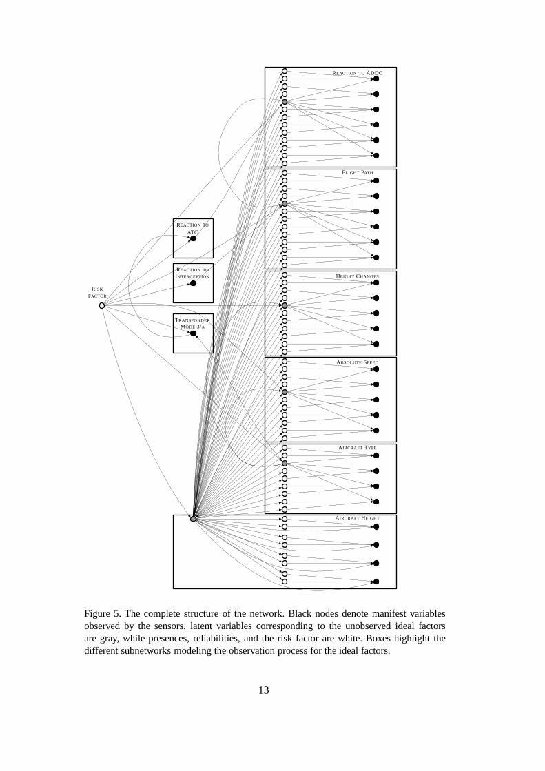
Whole Network The procedure considered in the previous paragraph for thenode AIRCRAFT TYPE is applied to every latent variable requiring informationfusion from many sensors. This practically means that we adda subnetwork simi-lar to the one reported in Fig. 4 to each light gray node of the network core in Fig. 2.The resulting directed graph, which is still acyclic, is shown in Fig. 5. A more com-pact specification could be obtained by extending the formalism ofobject-orientedBayesian networks[12] to credal networks. Accordingly, we can regard the boxedsubnetworks in Fig. 5, modeling the observations of the ideal factors, as differ-ent instances of a given class, for which appropriate specifications of the attributes(possible values, number of sensors, etc.) have been provided.

10 Here the RELIABILITY is intended as a global descriptor of the sensor performances.The quality of a particular observation can be clearly affected by the value of the idealvariable, but this is modeled in the relation between the latent and the ideal variable.

12

A IRCRAFT HEIGHT

A IRCRAFT TYPE

ABSOLUTE SPEED

HEIGHT CHANGES

FLIGHT PATH

REACTION TO ADDC

TRANSPONDER

MODE 3/A

REACTION TO

ATC

REACTION TO

INTERCEPTION

RISK

FACTOR

Figure 5. The complete structure of the network. Black nodesdenote manifest variablesobserved by the sensors, latent variables corresponding tothe unobserved ideal factorsare gray, while presences, reliabilities, and the risk factor are white. Boxes highlight thedifferent subnetworks modeling the observation process for the ideal factors.

13

5 Quantitative Assessment of the Network

As outlined in Sect. 3, the specification of a credal network over the variables as-sociated to the directed acyclic graph in Fig. 5 requires thespecification of a con-ditional credal set for each variable and each possible configuration of its parents.Specific procedures for the quantification of these credal sets based on Expert’squalitative judgements have been developed for the core variables (Sect. 5.1) andfor the nodes modeling the observation process (Sect. 5.2).

5.1 Quantification of the Network Core

Because of the scarcity of historical cases, the quantification of the conditionalcredal sets for the core variables in Fig. 2 is mainly based upon military and tech-nical considerations. The Expert provided a number of qualitative judgements like“erroneous intruders are light aircrafts with good chance”and“erroneous intrud-ers are business jets with little chance”, later translated into the following specifi-cations for the bounds of the probability intervals:

P (light aircraft|erroneous) ≥ .65,

P (business jet|erroneous) ≤ .20.

This kind of elicitation has been obtained following Walley’s guidelines for thetranslation of natural language judgements [21, p. 48]. Clearly, there is a degree ofarbitrariness in choosing single numbers for the bounds of the probability intervals,but much less than in similar approaches based on precise probabilities.

In some situations, the Expert was also able to identify logical constraint amongthe variables. As an example, the fact that“balloons cannot maintain high levels ofheight” represents a constraint between the possible values of the variables AIR-CRAFT TYPE and AIRCRAFT HEIGHT, that can be embedded into the structure ofthe network by means of the following zero probability assessment:

P (very high|balloon) = 0.

Overall, the conditional credal sets corresponding to elicited probability intervalshave been computed according to the procedure outlined in Sect. 3.1 and a well-defined credal network over the graphical structure in Fig. 2has been concluded.

14

5.2 Observations, Presence and Reliability

To complete the quantification of the credal network over thewhole graphical struc-ture in Fig. 5, we should discuss, for each sensor, the quantification of the variablesmodeling the observation process.

We begin by explaining how PRESENCEand RELIABILITY are specified. Considerthe network in Fig. 3. The Expert should quantify, for each ofthe four possiblevalues of AIRCRAFT HEIGHT, two credal sets, one for the PRESENCEand one forthe RELIABILITY . For the first, he takes into consideration only the structure of theidentification architecture; while for the second, also theactual meteorological andgeographical situation should be considered.

In principle, this quantification task would require that the Expert answer ques-tions like,“what is the probability (interval) that the ground-based observers havescarce (or medium, or high) reliability in observing an aircraft flying at low height,if the meteorological condition is characterized by dense low clouds and we are inthe plateau?”. Clearly, it can be extremely difficult and time-consuming to answerdozens of questions of this kind in a coherent and realistic way. For this reason, wesimply ask the Expert to providecharacteristic levelsof PRESENCEand RELIABIL -ITY . That can be obtained by questions like the following,“what is the reliabilitylevel that you expect from ground-based observations of an aircraft flying at lowheight, if the meteorological condition is characterized by dense low clouds and weare in the plateau?”. The latter question is much simpler, because one is requiredto specify something more qualitative than probabilities.Together with the charac-teristic levels, the Expert also indicates whether or not heis uncertain about thesevalues. Finally, for each combination of expected levels and relative uncertainty, afixed credal set is defined together with the Expert. That substantially simplifies thequantification task, while maintaining a large flexibility in the specification of themodel. As an example, assuming that Expert’s expected levelof reliability is highwith no uncertainty, a degenerate (precise) specification is adopted, i.e.,

P (RELIABILITY = high|A IRCRAFT HEIGHT = low) = 1;

while, in case of uncertainty about such expected level, an interval [.9, 1] is con-sidered instead, and a corresponding non-zero probabilityfor the medium level ofreliability should be assumed. Analogous procedures have been employed for thequantification of the PRESENCE.

Regarding the observations, a conditional credal set for each possible value of thecorresponding latent variable and each possible level of RELIABILITY and PRES-ENCE should be assessed.

Let X be a latent variable denoting an ideal factor andO the manifest variablecorresponding to the observation ofX as returned by a given sensor. For each

15

possible joint value of RELIABILITY and PRESENCE, say(r, p), we should assesslower and upper bounds forP (O = o|X = x, r, p), for eachx ∈ ΩX ando ∈ ΩO =ΩX ∪ ∗, and then compute the corresponding credal sets.

This quantification step can be simplified by defining a symmetric non-transitiverelation ofsimilarity among the elements ofΩX . The similarities between the pos-sible values of a latent variable according to a specific sensor can be naturally repre-sented by an undirected graph as in the example of Fig. 6. In general, given a latentvariableX, we ask the Expert to determine, for each possible outcomex ∈ ΩX , theoutcomes ofX that are similar tox and those that are not similar tox.

jet airliner helicopter

lightaircraft

glider balloon

Figure 6. An undirected graph depicting similarity relations about the possible values ofthe variable AIRCRAFT TYPE according to the observation of a TV camera. Edges connectsimilar states. The sensor can mix up alight aircraftwith aglider or ajet, butnot with aballoon or ahelicopter or anairliner.

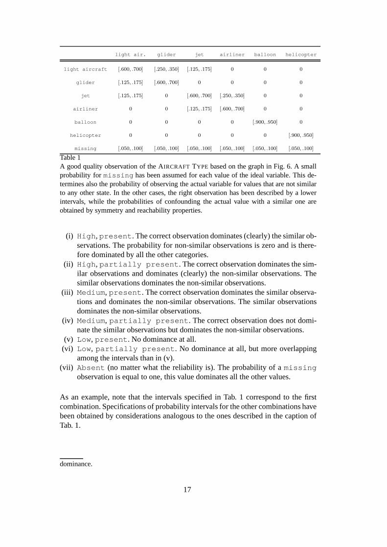
Having defined, for each latent variable and each corresponding sensor, the similar-ities between its possible outcomes, we can then divide the possible observations infour categories: (i) observing the actual value ofX; (ii) confounding the real valueof X with a similar one; (iii) confounding the actual value ofX with a value that isnot similar; (iv) the observation ismissing. The idea is to quantify, instead of aprobability interval forP (O = o|X = x, p, r) for eachx ∈ ΩX and eacho ∈ ΩO,only four probability intervals, corresponding to the fourcategories of observationsdescribed above. As an example, Tab. 1 reports an interval-valued quantificationof the conditional probability tableP (O|X, p, r) for the ideal variable AIRCRAFT

TYPE, for a combination(p, r) of the values of PRESENCEand RELIABILITY thatmodels a good (although not perfect) observation process.

Let us finally explain how the four probability intervals arequantified in our net-work for each combination of RELIABILITY and PRESENCEand each sensor. Theprobability interval assigned to the case where the observation is missing de-pends uniquely on the PRESENCE. In particular, the valueabsent, makes theprobability of having amissing observation equal to one and therefore the prob-ability assigned to all the other cases are equal to zero. It follows that we have onlyseven combinations of RELIABILITY and PRESENCEto quantify. To this extent, weuse constraints based on the concept ofinterval dominanceto characterize the dif-ferent combinations.11 In order of accuracy of the observation, the combinationsare the following:

11 Given a credal setK(X) over a variableX, and two possible valuesx, x′ ∈ ΩX , we saythat thex dominatesx′ if P (X = x′) < P (X = x) for eachP ∈ K(X). It is easy toshow that interval dominance, i.e.,P (X = x′) < P (X = x), is a sufficient condition for

16

light air. glider jet airliner balloon helicopter

light aircraft [.600, .700] [.250, .350] [.125, .175] 0 0 0

glider [.125, .175] [.600, .700] 0 0 0 0

jet [.125, .175] 0 [.600, .700] [.250, .350] 0 0

airliner 0 0 [.125, .175] [.600, .700] 0 0

balloon 0 0 0 0 [.900, .950] 0

helicopter 0 0 0 0 0 [.900, .950]

missing [.050, .100] [.050, .100] [.050, .100] [.050, .100] [.050, .100] [.050, .100]

Table 1A good quality observation of the AIRCRAFT TYPE based on the graph in Fig. 6. A smallprobability formissing has been assumed for each value of the ideal variable. This de-termines also the probability of observing the actual variable for values that are not similarto any other state. In the other cases, the right observationhas been described by a lowerintervals, while the probabilities of confounding the actual value with a similar one areobtained by symmetry and reachability properties.

(i) High,present. The correct observation dominates (clearly) the similar ob-servations. The probability for non-similar observationsis zero and is there-fore dominated by all the other categories.

(ii) High, partially present. The correct observation dominates the sim-ilar observations and dominates (clearly) the non-similarobservations. Thesimilar observations dominates the non-similar observations.

(iii) Medium, present. The correct observation dominates the similar observa-tions and dominates the non-similar observations. The similar observationsdominates the non-similar observations.

(iv) Medium, partially present. The correct observation does not domi-nate the similar observations but dominates the non-similar observations.

(v) Low, present. No dominance at all.(vi) Low, partially present. No dominance at all, but more overlapping

among the intervals than in (v).(vii) Absent (no matter what the reliability is). The probability of amissing

observation is equal to one, this value dominates all the other values.

As an example, note that the intervals specified in Tab. 1 correspond to the firstcombination. Specifications of probability intervals for the other combinations havebeen obtained by considerations analogous to the ones described in the caption ofTab. 1.

dominance.

17

6 Information Fusion by Imprecise Probabilities

The procedure described in Sect. 4.2 and 5.2 in order to mergethe observationsgathered by different sensors can be regarded as a possible imprecise-probabilityapproach to the generalinformation fusionproblem. In this section, we take a shortdetour from the military aspects to illustrate some key features of such an approachby simple examples.

Let us first formulate the general problem. Given a latent variableX, and the man-ifest variablesO1, . . . , On corresponding to the observations ofX returned bynsensors, we want to update our beliefs aboutX, given the valueso1, . . . , on re-turned by the sensors.

The most common way to solve this problem is to assess a (precise) probabilisticmodel over these variables, from which the conditional probability mass functionP (X|o1, . . . , on) can be computed. That may be suited to model situations of rel-ative consensusamong the different sensors. The precise models tend to assignhigher probabilities to the values ofX returned by the majority of the sensors,which may be a satisfactory mathematical description of these scenarios.

The problem is more complex in case ofdisagreementamong the different sen-sors. In these situations, precise models assign similar posterior probabilities to thedifferent values ofX. But a uniform posterior probability mass function seems tomodel a condition ofindifference(i.e., we trust the different observed values withthe same probability), while sensors disagreement reflectsinstead a condition ofignorance(i.e., we do not know which is the most likely value among the observedones).

Imprecise-probability models are more suited for these situations. Posterior igno-rance aboutX can be represented by the impossibility of a precise specificationof the conditional mass functionP (X|o1, . . . , on). The more disagreement we ob-serve among the sensors, the wider we expect the posterior intervals to be, for thedifferent values ofX.

The case where the bounds of a conditional probability strictly contain those of thecorresponding unconditional probability, and that happens for all the conditionalevents of a partition, is known in literature asdilation [16], and is relatively com-mon with coherent imprecise probabilities.

The following small example, despite its simplicity, is sufficient to outline howthese particular features are obtained by our approach.

Example 1Consider a credal network over a latent variableX, and two manifestvariablesO1 and O2 denoting the observations ofX returned by two identicalsensors. Assume to be given the strong independencies codedby the graph in Fig. 7.

18

Let all the variables be Boolean. AssumeP (X) uniform and bothP (Oi = 1|X =1) andP (Oi = 0|X = 0) to take values in the interval[1−γ, 1−ǫ], for each i=1,2,where the two parameters0 < ǫ < γ < .5 model a (small) error in the observationprocess. Since the network in Fig. 7 can be regarded as anaive credal classifier,where the latent variableX plays the role of the class node and the observationscorrespond to the class attributes, we can exploit the algorithm presented in [22,Sect. 3.1] to compute the following posterior intervals:

P (X = 1|O1 = 1, O2 = 1) ∈

1

1 + ( γ

1−γ)2

,1

1 + ( ǫ1−ǫ

)2

≃ [.941, .988],

P (X = 1|O1 = 1, O2 = 0) ∈

1

1 + γ(1−ǫ)ǫ(1−γ)

,1

1 + ǫ(1−γ)γ(1−ǫ)

≃ [.308, .692],

where the numerical values have been computed forǫ = .1, γ = .2. Note thatfor these specific values, as well as in the general case, the first interval is strictlygreater than.5, a value that represents the middle point of the second interval.Thus, we can conclude that: (i) consensus between the sensors increases the pos-terior probability for X; (ii) disagreement increases our ignorance aboutX (theprobability dilates).12

X

O1 O2

Figure 7. The credal network for Example 1.

These calculi can be easily generalized to the case ofn sensors. As an example,Fig. 8 depicts the posterior intervals for the observation of a Boolean latent variableby nine identical sensors for different levels of consensusamong them. Note thatour approach based on credal networks reproduces the cautious behaviour we wantto model, while a Bayesian network would abruptly change itsestimates with thenumber of correct observations passing from four to five. Unlike the imprecise case,precise conditional probabilities might therefore produce unreliable extreme valuesin the posterior beliefs because of high sensitivity to small changes in the error rate.

It should be also pointed out that the only assumption required by this approach isthe conditional independence between the manifest variables (observations) given

12 The valueǫ = 0 has been excluded, as it models a situation where both the sensors can beperfectly reliable. Clearly, such a scenario is not compatible with a disagreement betweenthe observations.

19

m

0 1 2 3 4 5 6 7 8 9

00.5

1

Figure 8. Posterior intervals forP (X = 1|O1 = 1, . . . , Om = 1, Om+1 = 0, . . . O9 = 0)as a function ofm, assuming bothP (Oj = 1|X = 1) andP (Oj = 0|X = 0) ∈ [.8, .9], foreachj = 1, . . . , 9, and a uniformP (X). Black dots denote precise posterior probabilitiescomputed assuming the precise value.85 for the conditional probabilities.

the latent variable (actual value of the quantity to be measured). A condition whichseems to be verified in many concrete cases, as for example that of the militaryproblem we address in this paper.

In fact, assuming fixed levels of AIRCRAFT HEIGHT, RELIABILITY and PRES-ENCE, Fig. 4 reproduces the same structure of the prototypical example in Fig. 7,with four sensors instead of two. The same holds for any subnetwork modeling therelations between a latent variable and the relative manifest variables.

7 Algorithmic Issues and Simulations

The discussion in Sect. 4 and Sect. 5 led us to the specification of a credal network,associated to the graph in Fig. 5, defined over the whole set ofconsidered variables,i.e., core variables, observations collected by the different sensors, reliability andpresence levels.

At this point, we can evaluate the risk associated to an intrusion, by simply updatingthe probabilities for the four possible values of the risk factor, conditional on thevalues of the observations returned by the sensors.

20

The size of our credal network prevents an exact computationof the posterior prob-ability intervals.13 Approximate procedures should be therefore employed, unlesswe do not want to restrict our analysis to the core of the network by assumingperfectly reliable observations for all the ideal factors.

The high computational complexity of the updating problem on the whole networkshould be regarded as the mathematical counterpart of the difficulties experiencedby the military experts during the identification of the intruder. On the other side,when all the factors are observed in a perfectly reliable way, the goal of the intrudercan be easily detected, exactly as the mathematical task of updating the core of thenetwork is equivalent to computing class probabilities in anaive credal classifier,a task efficiently solved by the algorithm in [22].

Thus, we have first performed extensive simulations on the core of the network. Ex-pert has considered several combinations of values for the ideal factors and checkedwhether or not the set of undominated classes returned by thecore of the networkwas including his personal evaluation of the goal of an intruder for that scenario.Every time a mismatch between the human and the artificial expert was detected,the quantification of the probability for the network was updated. Remarkably, atthe end of this validation task, we have obtained a network core able to simulatethe Expert’s evaluation in almost every considered scenario.

Then, as a test for the whole network, we have considered a simulated restrictedflight area for the protection of a single object in the Swiss Alps, surveyed by anidentification architecture characterized by absence of interceptors and relativelygood coverage of all the other sensors. We assumed as meteorological conditionsdiscontinuous low clouds and daylight. The simulated scenario reproduces a situa-tion where a provocateur is flying very low with a helicopter and without emittingany identification code. The corresponding evidences are reported in Tab. 2.

In order to compute the posterior intervals we have considered an approximate al-gorithm calledgeneralized loopy 2U[2], whose performances in terms of accuracyand scalability seems to be quite good. The posterior intervals were computed infew seconds on a 2.8 GHz Pentium 4 machine.

For this simulation we have assumed uniform prior beliefs about the four classesof risk.14 Fig. 9.a depicts the posterior probability intervals for this simulated sce-nario. The upper probability for the outcomerenegade is zero, and we can there-fore exclude a terrorist attack. Similarly, the lower probability for the outcomesagent provocateur anddamaged are strictly greater than the upper proba-

13 The existing algorithms for exact updating of credal networks (e.g., [6,15]) are typicallytoo slow for models with dense topologies and more than 50 nodes.14 Any credal set can be used to model decision maker’s prior beliefs about the risk fac-tor. Nevertheless, as noted in [14], avacuousprior (i.e., a credal set equal to the wholeprobability simplex) would make vacuous also the posteriorinferences.

21

VARIABLE SENSOR1 SENSOR2 SENSOR3 SENSOR4 SENSOR5 SENSOR6

(SSR) (3D) (2D) (TV) (GROUND) (TRACK)

A IRCRAFT HEIGHT very low very low - - low very low / low

TYPE OFA IRCRAFT - - - helicopter helicopter -

FLIGHT PATH U-path U-path U-path U-path missing U-path

HEIGHT CHANGES descent descent descent - missing descent

ABSOLUTESPEED slow slow slow - slow slow

REACTION TO ADDC positive positive positive positive positive positive

Table 2Sensors observations for the simulations in Fig. 9. The AIRCRAFT HEIGHT according tothe tracking radar (SENSOR6) isvery low in (a) and (b), andlow in (c).

bility for the stateerroneous, and we can reject as less credible also this lattervalue because of interval dominance.

The ambiguity betweenagent provocateur anddamaged is due, in thiscase, to the bad observation of the AIRCRAFT HEIGHT. In fact, a damaged heli-copter is expected to land as soon as possible. While, in the modeled scenario, aprovocateur is not expected to land. With a bad observation of the height, we areunable to understand if the helicopter has landed or not and therefore the ambiguitybetween the two risk categories is reasonable.

Indecision betweenagent provocateur anddamaged disappears if we as-sume higher expected levels of RELIABILITY and PRESENCEfor the sensors de-voted to the observation of the AIRCRAFT HEIGHT. The results in Fig. 9.b statethat the intruder is anagent provocateur, as we have assumed in the designof this simulation.

In Fig. 9.c we still consider a high quality observation, butmore disagreementbetween the sensors (see Tab. 2). This produces, also in thiscase, indecision be-tween two classes. Remarkably, as we expect from our model ofthe informationfusion in case of disagreement, the intervals we observe seem to reproduce theunion of the intervals computed on the network core assumingrespectivelyverylow (Fig. 9.d) andlow (Fig. 9.e) AIRCRAFT HEIGHT.

Remarkably, these results have been recognized by the Expert as reasonable esti-mates for the considered scenarios. Yet, an extensive validation process, consist-ing in analyses of this kind by different military experts onmany other scenarios,should be regarded as a necessary future work.

22

prov

err

dam

0

1

1

2

1

4

3

4

(a)

prov

err

dam

(b)

prov

err

dam

(c)

prov

dam

(d)

prov dam

(e)

Figure 9. Posterior probability intervals for the risk factor, corresponding to the evidencesreported in Tab. 2. The histogram bounds denote lower and upper probabilities. The qualityof the observation of the AIRCRAFT HEIGHT is assumed to be higher in (b) than in (a).The histograms in (c) refers to a situation of increased disagreement between the sensorsobserving the AIRCRAFT HEIGHT. Finally, (d) and (e) report respectively the exact poste-rior intervals in a situation where the observation of the factors is assumed to be perfectlyreliable and corresponds to the value returned by the majority of the sensors.

8 Conclusions and Future Work

A model for determining the risk of intrusion of a civil aircraft into restricted flightareas has been presented. The model embeds in a single coherent mathematicalframework human expertise expressed by imprecise-probability assessments, and astructure reproducing complex observation processes and corresponding informa-tion fusion schemes.

The risk evaluation corresponds to the updating of the probabilities for the riskfactor conditional on the observations of the sensors and the estimated levels ofpresence and reliability. Preliminary tests considered for a simulated scenario areconsistent with the judgements of an expert domain for the same situation.

As future work we intend to test the model for other historical cases and simulatedscenarios. The approximate updating procedure consideredin the present work, aswell as other algorithmic approaches will be considered, inorder to determine themost suited for this specific problem.

In any case, it seems already possible to offer a practical support to the militaryexperts in their evaluations. They can use the network to decide the risk level corre-sponding to a real scenario, but it is also possible to simulate situations and verifythe effectiveness of the different sensors in order to design an optimal identificationarchitecture.

23

Finally, we regard our approach to the fusion of the information collected by thedifferent sensors as a sound and flexible approach to this kind of problems, able towork also in situations of contrasting observations between the sensors.

Acknowledgments

We are very grateful to the experts of Armasuisse and the Swiss Air Force for theirhelp and support and for the interesting discussions.

A Python/C++ software implementation of the generalized loopy 2U algorithm(http://www.idsia.ch/∼yi/gl2u.html) developed by Sun Yi has been used to updatethe credal networks. The software toollrs (http://cgm.cs.mcgill.ca/∼avis/C/lrs.htm)has been used to compute the vertices of the conditional credal sets correspondingto the probability intervals provided by the Expert. The authors of these publicsoftware tools are gratefully acknowledged.

References

[1] A. Antonucci and M. Zaffalon. Decision-theoretic specification of credal networks: Aunified language for uncertain modeling with sets of Bayesian networks.InternationalJournal of Approximate Reasoning, 49(2):345–361, 2008.

[2] A. Antonucci, M. Zaffalon, Y. Sun, and C.P. de Campos. Generalized loopy 2U: A newalgorithm for approximate inference credal networks. In M.Jaeger and T.D. Nielsen,editors,Proceedings of the Fourth European Workshop on Probabilistic GraphicalModels, pages 17–24, Hirtshals (Denmark), 2008.

[3] D. Avis and K. Fukuda. A pivoting algorithm for convex hulls and vertex enumerationof arrangements and polyhedra.Discrete and Computational Geometry, 8(3):295–313,1992.

[4] D. Boorsbom, G.J. Mellenbergh, and J. van Heerden. The theoretical status of latentvariables.Psychological Review, 110(2):203–219, 2002.

[5] L. Campos, J. Huete, and S. Moral. Probability intervals: a tool for uncertainreasoning. International Journal of Uncertainty, Fuzziness and Knowledge-BasedSystems, 2(2):167–196, 1994.

[6] A. Cano, M. Gomez, S. Moral, and J. Abellan. Hill-climbing and branch-and-boundalgorithms for exact and approximate inference in credal networks. InternationalJournal of Approximate Reasoning, 44(3):261–280, 2007.

[7] F.G. Cozman. Credal networks.Artificial Intelligence, 120:199–233, 2000.

24

[8] F.G Cozman. Graphical models for imprecise probabilities. International Journal ofApproximate Reasoning, 39(2-3):167–184, 2005.

[9] C.P. de Campos and F.G. Cozman. The inferential complexity of Bayesian and credalnetworks. InProceedings of the 19th International Joint Conference on ArtificialIntelligence, pages 1313–1318, Edinburgh, 2005.

[10] C.P. de Campos and Q. Ji. Strategy selection in influencediagrams using impreciseprobabilities. InProceedings of the 24th Conference on Uncertainty in ArtificialIntelligence, pages 121–128. AUAI Press, 2008.

[11] E. Demircioglu and L. Osadciw. A Bayesian network sensors manager forheterogeneous radar suites. InIEEE Radar Conference, Verona, NY, 2006.

[12] D. Koller and A. Pfeffer. Object-oriented Bayesian networks. InProceedings of the13th Conference on Uncertainty in Artificial Intelligence, pages 302–313, 1997.

[13] J. Pearl. Probabilistic Reasoning in Intelligent Systems: Networksof PlausibleInference. Morgan Kaufmann, San Mateo, 1988.

[14] A. Piatti, M. Zaffalon, F. Trojani, and M. Hutter. Learning about a categorical latentvariable under prior near-ignorance. In G. de Cooman, J. Vejnarova, and M. Zaffalon,editors,Proceedings of the 5th International Symposium on Imprecise Probability:Theories and Applications, pages 357–364, Prague, 2007. Action M.

[15] J.C. Rocha and Cozman F.G. Inference in credal networks: branch-and-bound methodsand the A/R+ algorithm.International Journal of Approximate Reasoning, 39:279–296, 2005.

[16] T. Seidenfeld and L. Wasserman. Dilation for sets of probabilities.Annals of Statistics,21(3):1139–1154, 1993.

[17] AIP Services.Aeronautical Information Publication Switzerland. Skyguide, 2007.

[18] A. Skrondal and S. Rabe-Hasketh.Generalized latent variable modeling: multilevel,longitudinal, and structural equation models. Chapman and Hall/CRC, Boca Raton,2004.

[19] B. Tessem. Interval probability propagation.International Journal of ApproximateReasoning, 7(3):95–120, 1992.

[20] P. Walley.Statistical Reasoning with Imprecise Probabilities. Chapman and Hall, NewYork, 1991.

[21] P. Walley. Measures of uncertainty in expert systems.Artificial Intelligence, 83(1):1–58, 1996.

[22] M. Zaffalon. The naive credal classifier.Journal of Statistical Planning and Inference,105(1):5–21, 2002.

25