Embed Size (px)
Citation preview

TECHNISCHE UNIVERSITAT MUNCHEN
Fachgebiet Organische Chemie
Creation of Novel Pulses forMagnetic Resonance by
Optimal Control
Manoj Manohar Nimbalkar
Vollstandiger Abdruck der von der Fakultat fur Chemie der Technischen UniversitatMunchen zur Erlangung des akademischen Grades eines
Doktors der Naturwissenschaften
genehmigten Dissertation.
Vorsitzender: Univ.-Prof. Dr. Bernd Reif
Prufer der Dissertation: 1. Univ.-Prof. Dr. Steffen J. Glaser
2. Univ.-Prof. Dr. Axel Haase
Die Dissertation wurde am 27.10.2011 bei der Technischen Universitat Munchen eingereichtund durch die Fakultat fur Chemie am 01.12.2011 angenommen.


i
!" к$% &' a($) a*+к$%। -.-$/$ 0)1$ш" &' %к$%।к13 a($)$43 4*56$%। &' !" % 76839.॥ 27॥
0;;.к04*+<
। a$и &" / >$?$ !" %।
The first letter “!" ” (Gu) of “!" %”, (Guru) Teacher, represents the darkness ofilliteracy, ignorance, unawareness. The second letter “%” (Ru) stands for theeradication of that darkness. Therefore, who brings/helps you from the darknessof ignorance towards the path of enlightenment is a true “!" %”.
Viveksindhu
My Mother has always guided me through the difficult situations and showedme the ways towards the right directions. Therefore, she is and will be my true“!" %”, who showed me the path toward the enlightenment.
1

ii

iii
!" #$ %&'( a$)" ,a*$ a$+, a$)-&$ .$'/$ 0!+123 к53-.
I dedicate this Thesis to my grandparents Aaji and Anna, and Aajoba.

iv

Declaration
I hereby declare that parts of this Thesis are already published/submitted or plannedto be submitted in scientific journals:
List of Publications
Linear phase slope in pulse design: Application to coherence transfer;Naum I. Gershenzon, Thomas E. Skinner, Bernhard Brutscher, Navin Khaneja,Manoj Nimbalkar, Burkhard Luy, Steffen J. Glaser, J. Magn. Reson., 192,
235-243 (2008).
Broadband 180◦ universal rotation pulses for NMR spectroscopy de-
signed by optimal control;Thomas E. Skinner, Naum I. Gershenzon, Manoj Nimbalkar, Wolfgang Bermel,Burkhard Luy, Steffen J. Glaser, arXiv: 1111.6647, J. Magn. Reson., in press,2011.
Optimal control design of band-selective excitation pulses that accom-
modate relaxation and RF inhomogeneity;Thomas E. Skinner, Naum I. Gershenzon, Manoj Nimbalkar, Steffen J. Glaser,arXiv: 1111.6650, J. Magn. Reson., submitted, 2011.
Multiple-spin coherence transfer in linear Ising spin chains and beyond:
numerically-optimized pulses and experiments;Manoj Nimbalkar, Robert Zeier, Jorge L. Neves, S. Begam Elavarasi, HaidongYuan, Navin Khaneja, Kavita Dorai, and Steffen J. Glaser, arXiv: 1110.5262,Phys. Rev. A, in press, 2011.
The Fantastic Four: A plug ‘n’ play set of optimal control pulses for
enhancing nmr spectroscopy;Manoj Nimbalkar, Burkhard Luy, Thomas E. Skinner, Jorge L. Neves, Naum I.Gershenzon, Kyryl Kobzar, Wolfgang Bermel, Steffen J. Glaser, in preparation.
v

vi
Eidesstattliche Versicherung
Ich versichere, dass ich die von mir vorgelegte Dissertation selbstandig angefertigt, diebenutzten Quellen und Hilfsmittel vollstandig angegeben und die Stellen der Arbeit, dieanderen Werken im Wortlaut oder dem Sinn nach entnommen sind, in jedem Einzelfallals Entlehnung kenntlich gemacht habe; dass diese Dissertation noch keiner anderenFakultat oder Universitat zur Prufung vorgelegen hat; dass sie abgesehen von untenangegebenen Teilpublikationen noch nicht veroffentlicht worden ist sowie, dass ich einesolche Veroffentlichung vor Abschluss des Promotionsverfahrens nicht vornehmen werde.Die Bestimmungen dieser Promotionsordnung sind mir bekannt. Die von mir vorgelegteDissertation ist von Herrn Prof. Dr. S. J. Glaser betreut worden.
Publikationsliste
Linear phase slope in pulse design: Application to coherence transfer;Naum I. Gershenzon, Thomas E. Skinner, Bernhard Brutscher, Navin Khaneja,Manoj Nimbalkar, Burkhard Luy, Steffen J. Glaser, J. Magn. Reson., 192,
235-243 (2008).
Broadband 180◦ universal rotation pulses for NMR spectroscopy de-
signed by optimal control;Thomas E. Skinner, Naum I. Gershenzon, Manoj Nimbalkar, Wolfgang Bermel,Burkhard Luy, Steffen J. Glaser, arXiv: 1111.6647, J. Magn. Reson., in press,2011.
Optimal control design of band-selective excitation pulses that accom-
modate relaxation and RF inhomogeneity;Thomas E. Skinner, Naum I. Gershenzon, Manoj Nimbalkar, Steffen J. Glaser,arXiv: 1111.6650, J. Magn. Reson., submitted, 2011.
Multiple-spin coherence transfer in linear Ising spin chains and beyond:
numerically-optimized pulses and experiments;Manoj Nimbalkar, Robert Zeier, Jorge L. Neves, S. Begam Elavarasi, HaidongYuan, Navin Khaneja, Kavita Dorai, and Steffen J. Glaser, arXiv: 1110.5262,Phys. Rev. A, in press, 2011.
The Fantastic Four: A plug ‘n’ play set of optimal control pulses for
enhancing nmr spectroscopy;Manoj Nimbalkar, Burkhard Luy, Thomas E. Skinner, Jorge L. Neves, Naum I.Gershenzon, Kyryl Kobzar, Wolfgang Bermel, Steffen J. Glaser, in preparation.
vii

viii

Abstract
This thesis is concerned with developing, optimizing, and implementing shaped pulsesand pulse sequences using the principles of optimal control theory (Chapter 2). It helpsto solve some of the most basic yet important problems in nuclear magnetic resonance(NMR) spectroscopy and magnetic resonance imaging (MRI), such as inhomogeneity inthe radio frequency (RF) fields delivered to the sample, the need for large chemical shiftbandwidth, and loss of signal intensity due to relaxation.
Considering the specific application for high-field NMR spectroscopy Chapter 3presents robust broadband excitation pulses optimized using optimal control methodswith a defined linear phase dispersion. This makes it possible to create pulses that areequivalent to ideal hard pulses followed by an effective evolution period. Chapter 4introduces new modifications of the optimal control algorithm that incorporate sym-metry principles and relax conservative limits on peak RF pulse amplitude for shorttime periods to generate a set of broadband universal rotation pulses. They are suitablefor widespread use in carbon spectroscopy on the majority of available probes.
Chapter 5 puts forth relaxation-compensated and RF-inhomogeneity robust selectiveexcitation pulses for short longitudinal (T1) and transverse (T2) relaxation equal to thepulse length, which reduces signal loss significantly while achieving nearly ideal frequencyselectivity. Improvements in performance are the result of allowing residual unrefocusedmagnetization after applying relaxation-compensated selective excitation by optimizedpulses (RC-SEBOP).
Chapter 6 presents numerical approaches to create multiple (3-6) spin coherence forspins-1/2 in multi-dimensional NMR experiments for Ising coupled three to six spins-1/2 with equal and unequal couplings. These pulses are significantly shorter in dur-ation compared to conventional pulse sequences. Utilizing the DANTE approach theshaped pulses were made broadband and implemented experimentally and comparedwith conventional pulse sequences to create the desired coherence order for three andfour spins-1/2 systems.
The last Chapter 7 is about “Fantastic Four” (Fanta4) pulses, a set of highly robust,optimal control-based shaped pulses that are able to replace all hard pulses (in one-to-one fashion) in pulse sequences consisting of 90◦ and 180◦ pulses for better performance.The set of four pulses for each nucleus consists of point-to-point (PP) 90◦ and 180◦, anduniversal rotation (UR) 90◦ and 180◦ pulses of identical duration (1 ms).
ix

x

Zusammenfassung
Diese Arbeit befasst sich mit der Entwicklung, Optimierung und Implementierung vongeformten Pulsen und Pulssequenzen, die Prinzipien aus der optimalen Steuerungsthe-orie verwenden (Kapitel 2). Sie tragt dazu bei, einige der grundlegendsten und zugleichwichtigsten Probleme der NMR-Spektroskopie und der MR-Bildgebung zu losen, wiezum Beispiel Inhomogenitat der auf die Probe eingestrahlten Radiofrequenz-Felder, derBedarf fur große chemische Verschiebungsbandbreite und relaxationsbedingter Verlustder Signalintensitat.
Unter Beachtung spezifischer Anwendungen fur die Hochfeld-NMR-Spektroskopiewerden in Kapitel 3 robuste und breitbandige Anregungspulse vorgestellt, die unterVerwendung von Methoden der optimalen Steuerungstheorie optimiert wurden und einelineare Phasendispersion aufweisen. Dies ermoglicht die Erzeugung von Pulsen, die sichaquivalent verhalten, wie ein idealer harter Puls gefolgt von einem effektiven Evolu-tionsdelay. In Kapitel 4 werden neue Modifikationen des optimalen Steuerungsalgorith-mus vorgestellt, die Symmetrieprinzipien berucksichtigen und konservative Beschrankun-gen der hochstmoglichen RF-Pulsamplitude fur kurze Zeitabschnitte lockern, um eineGruppe von breitbandigen universellen Rotationspulsen zu erzeugen. Sie sind fur vielfal-tige Anwendungen in der Kohlenstoffspektroskopie und fur die Mehrzahl der gangigenProbenkopfe geeignet.
In Kapitel 5 werden relaxationskompensierte und RF-Inhomogenitats-robuste selekti-ve Anregungspulse vorgestellt deren Pulsdauer gleich der longitudinalen T1 und trans-versalen T2 Relaxationszeiten sind. Dadurch wird der Signalverlust singifikant reduziertund gleichzeitig eine nahezu ideale Frequenzselektivitat erreicht. Verbesserte Ergebnissekonnen dadurch erzielt werden, dass nicht refokussierte Magnetisierung nach Anwendungeines relaxationskompensierten selektiven Anregungspulses (relaxation-compensated se-lective excitation by optimized pulses, RC-SEBOP) zugelassen wird.
In Kapitel 6 werden numerische Verfahren zur Erzeugung von mehrfachen (3-6)Spinkoharenzen fur Spin-1/2-Systeme in mehrdimensionalen NMR-Experimenten furdrei und sechs Ising-Spins 1/2 mit gleichen und unterschiedlichen Kopplungen vorge-stellt. Diese Pulse weisen im Vergleich zu konventionellen Pulsequenzen deutlich kurzerePulsdauern auf. Unter Verwendung des DANTE-Verfahrens wird die Breitbandigkeitdieser Pulse erhoht. Sie werden experimentell implementiert und mit einer konventio-nellen Pulssequenz verglichen, die die gewunschte Koharenzordnung fur ein drei- undein vier-Spin-1/2-System erzeugt.
Das letzte Kapitel 7 behandelt “Fantastic Four” (Fanta4) Pulse, eine Gruppe vonbesonders robusten und auf optimaler Steuerungstheorie basierenden Pulsen, die (”eins-zu-eins”) alle harten 90◦ und 180◦ Pulse in Pulssequenzen ersetzen konnen, um einebessere Leistung zu erzielen. Die Gruppe von vier Pulsen fur jeden Kern besteht ausPunkt-zu-Punkt (PP) 90◦ und 180◦ Pulsen und aus universellen 90◦ und 180◦ Rotation-spulsen (UR) gleicher Dauer (1 ms).
xi

xii

Acknowledgements
I would like to thank all with whom I worked during my thesis. I would like to givespecial thanks to Burkhard Luy, Jorge L. Neves, Kyryl Kobzar and Nikolas Pomplumfor their initial help and also to Raimond Marx, Andreas Sporl, Robert Fischer, UweSander, Grit Kummerlowe, Jochen Klages, Arnaud Ngongang Djintchui, Xiaodong Yang,Michael Braun, Martin Janich, Dr. Rainer Haeßner, Dr. Gerd Gemmecker, AdelinePalisse, Ariane Garon, Mirjam Holbach, Martha Fill, and rest of Glaser group; Kesselergroup; Luy group. I would like to thank my theoretical collaborators, Robert Zeier,Navin Khaneja, Naum I. Gershenzone, and special thank to Thomas E. Skinner for hisadvice. I would like to thank Dr. Wolfgang Eisenreich for allowing to use spectrometerat their facility in Department of Chemie, TUM. I would like to thank Bayerisches NMRZentrum. I would like to thank TUM Graduate school. I am very greatful to all myfriends, teachers and others whom I did not mentioned here.
Without saying I am very grateful to my family (Aai, Pappa, Dada and Vaini,Vashutai and bhauji, and Balutai and jiju, mothe Mama and Mami, Mama and Mami,and all other) and for their moral support, motivation, and encouragement.
Finally, I would like to thank Prof. Steffen J. Glaser for his exceptional supervision.
xiii

xiv

Contents
1 Prologue 1
1.1 Prospect . . . . . . . . . . . . . . . . . . . . . . . . . . . . . . . . . . . . . 11.2 Lay out of thesis . . . . . . . . . . . . . . . . . . . . . . . . . . . . . . . . 11.3 Synopsis of Chapters . . . . . . . . . . . . . . . . . . . . . . . . . . . . . . 2
2 Optimal control methodologies 5
2.1 Introduction . . . . . . . . . . . . . . . . . . . . . . . . . . . . . . . . . . . 52.2 Optimal control using Bloch equation . . . . . . . . . . . . . . . . . . . . 5
2.2.1 Classical Euler-Lagrange formalism . . . . . . . . . . . . . . . . . . 62.2.2 Optimal control algorithm without relaxation . . . . . . . . . . . . 62.2.3 Optimal control algorithm with relaxation . . . . . . . . . . . . . . 7
2.3 Optimal control using Liouville-von Neuman equation . . . . . . . . . . . 8
3 Linear phase slope in pulse design 11
3.1 Introduction . . . . . . . . . . . . . . . . . . . . . . . . . . . . . . . . . . . 113.2 Phase Slope . . . . . . . . . . . . . . . . . . . . . . . . . . . . . . . . . . . 123.3 Optimal control algorithm . . . . . . . . . . . . . . . . . . . . . . . . . . . 123.4 Applications . . . . . . . . . . . . . . . . . . . . . . . . . . . . . . . . . . . 13
3.4.1 Shorter broadband excitation . . . . . . . . . . . . . . . . . . . . . 133.4.2 Coherence transfer . . . . . . . . . . . . . . . . . . . . . . . . . . . 133.4.3 Experimental . . . . . . . . . . . . . . . . . . . . . . . . . . . . . . 14
3.5 Conclusion . . . . . . . . . . . . . . . . . . . . . . . . . . . . . . . . . . . 15
4 Broadband 180◦ universal rotation pulses 21
4.1 Introduction . . . . . . . . . . . . . . . . . . . . . . . . . . . . . . . . . . . 214.2 Optimal control algorithm for 180◦UR pulses . . . . . . . . . . . . . . . . . 22
4.2.1 Flavor I (basic vanilla) . . . . . . . . . . . . . . . . . . . . . . . . . 224.2.2 Flavor II (symmetry principle) . . . . . . . . . . . . . . . . . . . . 234.2.3 Flavor III (time-dependent RF limit) . . . . . . . . . . . . . . . . . 23
4.3 BURBOP compared to refocusing with PP pulses . . . . . . . . . . . . . . 234.3.1 Algorithms AT and AS,T . . . . . . . . . . . . . . . . . . . . . . . 24
4.4 Experiment . . . . . . . . . . . . . . . . . . . . . . . . . . . . . . . . . . . 274.5 Conclusion . . . . . . . . . . . . . . . . . . . . . . . . . . . . . . . . . . . 27
5 Band-selective excitation pulses
that accommodate relaxation and RF inhomogeneity 35
5.1 Introduction . . . . . . . . . . . . . . . . . . . . . . . . . . . . . . . . . . . 355.2 Selective pulse design . . . . . . . . . . . . . . . . . . . . . . . . . . . . . . 36
5.2.1 Phase slope . . . . . . . . . . . . . . . . . . . . . . . . . . . . . . . 36
xv

xvi CONTENTS
5.2.2 Selective pulses as digital filters . . . . . . . . . . . . . . . . . . . . 375.2.3 Optimal control . . . . . . . . . . . . . . . . . . . . . . . . . . . . . 37
5.3 Results and Discussion . . . . . . . . . . . . . . . . . . . . . . . . . . . . . 385.3.1 Tolerance to RF inhomogeneity . . . . . . . . . . . . . . . . . . . . 395.3.2 Compensation for relaxation and RF inhomogeneity . . . . . . . . 39
5.4 Experimental . . . . . . . . . . . . . . . . . . . . . . . . . . . . . . . . . . 445.5 Conclusion . . . . . . . . . . . . . . . . . . . . . . . . . . . . . . . . . . . 48
6 Time optimal pulses for multiple-spin coherence transfer 49
6.1 Introduction . . . . . . . . . . . . . . . . . . . . . . . . . . . . . . . . . . . 496.2 Coherence transfer in linear Ising spin chains . . . . . . . . . . . . . . . . 516.3 Linear three-spin chains: analytic and numerical approaches . . . . . . . . 52
6.3.1 Analytic approach . . . . . . . . . . . . . . . . . . . . . . . . . . . 526.3.2 Numerical approach . . . . . . . . . . . . . . . . . . . . . . . . . . 53
6.4 Linear four-spin chains: analytic and numerical approaches . . . . . . . . 556.4.1 Analytic approach . . . . . . . . . . . . . . . . . . . . . . . . . . . 556.4.2 Numerical approach . . . . . . . . . . . . . . . . . . . . . . . . . . 56
6.5 More generally-coupled spin systems of three and four spins . . . . . . . . 576.5.1 Three-spin system . . . . . . . . . . . . . . . . . . . . . . . . . . . 586.5.2 Four-spin system . . . . . . . . . . . . . . . . . . . . . . . . . . . . 58
6.6 Experimental results . . . . . . . . . . . . . . . . . . . . . . . . . . . . . . 586.6.1 Conventional pulse sequences . . . . . . . . . . . . . . . . . . . . . 64
6.7 Linear spin chains with more than four spins . . . . . . . . . . . . . . . . 646.8 Conclusion . . . . . . . . . . . . . . . . . . . . . . . . . . . . . . . . . . . 65
7 The Fantastic Four: A plug ‘n’ play set of optimal control pulses 67
7.1 Introduction . . . . . . . . . . . . . . . . . . . . . . . . . . . . . . . . . . . 677.2 Optimization . . . . . . . . . . . . . . . . . . . . . . . . . . . . . . . . . . 697.3 Experiments . . . . . . . . . . . . . . . . . . . . . . . . . . . . . . . . . . . 707.4 Results . . . . . . . . . . . . . . . . . . . . . . . . . . . . . . . . . . . . . . 70
7.4.1 HSQC: Testing with Sodium Formate . . . . . . . . . . . . . . . . 707.4.2 HSQC: Testing with Hydroxycitronellal . . . . . . . . . . . . . . . 707.4.3 HMBC: Testing on Real molecule . . . . . . . . . . . . . . . . . . . 73
7.5 Discussion . . . . . . . . . . . . . . . . . . . . . . . . . . . . . . . . . . . . 737.6 Conclusion . . . . . . . . . . . . . . . . . . . . . . . . . . . . . . . . . . . 787.7 Appendix . . . . . . . . . . . . . . . . . . . . . . . . . . . . . . . . . . . . 78
7.7.1 Optimization of pulse pairs for two coupled heteronuclear spins-1/2 787.7.2 Fanta4 pulse selection . . . . . . . . . . . . . . . . . . . . . . . . . 797.7.3 Fanta4 pulse shapes and excitation profiles . . . . . . . . . . . . . 82

Abbreviations
• NMR: Nuclear Magnetic Resonance
• MRI: Magnetic Resonance Imaging
• RF: Radio Frequency
• B01 : Nominal RF amplitude
• T1: Longitudinal relaxation time
• T2: Transverse relaxation time
• RC-SEBOP: Relaxation-Compensated Selective Excitation by Optimized Pulse
• DANTE: Delays Alternating with Nutations for Tailored Excitation
• Fanta4: Flavored rf and offset robust Alike-duration Numerically-optimized Trouble-free Applicable 4 pulses
• PP: Point to point pulse
• UR: Universal Rotation pulse
• B0: The Static magnetic field
• ICEBERG: Inherent Coherence Evolution optimized Broadband Excitation Res-ulting in constant phase Gradients
• BURBOP: Broadband Universal Rotation by Optimized Pulses
• EPR: Electron Spin Resonance
• DNP: Dynamic Nuclear Polarization
• HMQC: Heteronulcear Multiple Quantum Coherence
• RFmax: Maximum RF amplitude
• Tp or tp: Total pulse duration
• FIR: Finite Impulse Response
• BW: Band Width
• SLR: Shinnar-LeRoux algorithm
• COSY: Correlation Spectroscopy
xvii

xviii CONTENTS
• INEPT: Insensitive Nuclei Enhanced by Polarization Transfer
• GRAPE: Gradient Ascent Pulse Engineering
• TOP: Time Optimal Pulse curve
• HSQC: Heteronuclear Single Quantum Coherence
• HMBC: Heteronuclear Multiple-Bond Coherence
• INADEQUATE: Incredible Natural Abundance Double Quantum Transfer Exper-iment
• NOESY: Nuclear Overhauser Enhancement Spectroscopy

List of Figures
2.1 Optimization scheme. . . . . . . . . . . . . . . . . . . . . . . . . . . . . . 8
3.1 Performance of a 16.7 µs hard pulse. . . . . . . . . . . . . . . . . . . . . . 143.2 Amplitude-modulated pulse of length 39 µs and peak RF amplitude = 15
kHz, optimized to excite transverse magnetization Mxy with linear phaseslope R = 1/2 over resonance offsets of 50 kHz. . . . . . . . . . . . . . . . 15
3.3 The use of a linear phase slope pulse to reduce the delay τ in selectivecoherence transfer in the case where Tp is relatively long. . . . . . . . . . 16
3.4 The RF amplitude and Phase are plotted for ICEBERG pulses of R =-0.5 to 0.95. . . . . . . . . . . . . . . . . . . . . . . . . . . . . . . . . . . 17
3.5 Excitation profile of ICEBERG pulses with different R compared withhard pulse (Tp = 16.7 µs) . . . . . . . . . . . . . . . . . . . . . . . . . . . 18
3.6 Creation of ICEBERG-HMQC from conventional HMQC. . . . . . . . . . 193.7 Experimental comparison of ICEBERG-HMQC and hard pulse HMQC . . 20
4.1 The amplitude and phase of adiabatic Chirp80 pulse from Bruker pulselibrary. . . . . . . . . . . . . . . . . . . . . . . . . . . . . . . . . . . . . . 25
4.2 The amplitude and phase of 180◦UR pulse 4 from Table 1 obtained usingalgorithm AS,T . . . . . . . . . . . . . . . . . . . . . . . . . . . . . . . . . . 25
4.3 Theoretical performance of four 180◦UR pulses for inversion of magnetiza-tion about the y-axis, designed using different algorithms. . . . . . . . . . 26
4.4 Theoretical performance of pulse 1 and pulse 4 of Table, and compositeadiabatic pulse for inversion of magnetization about the y-axis. . . . . . . 28
4.5 Simulations: Further quantitative detail for the Mx → −Mx transforma-tion from Fig. 4.4b for pulse 4 of Table 1 and Fig. 4.4c for Chirp80. . . . . 29
4.6 Experimental measurements of the inversion profile and phase deviationfor pulse 4 of Table 1 and adiabatic Chirp80. . . . . . . . . . . . . . . . . 30
4.7 Experimental lineshapes (black) comparing optimal control 180◦UR pulse4 of Table 1 and adiabatic Chirp80. . . . . . . . . . . . . . . . . . . . . . . 31
4.8 Simulations: Further quantitative detail for theMy → My transformationfrom Fig. 4.4b for pulse 4 of Table 1 and Fig. 4.4c for Chirp80. . . . . . . 32
4.9 Experimental measurements of the My → My and phase deviation forpulse 4 of Table 1 and adiabatic Chirp80. . . . . . . . . . . . . . . . . . . 33
4.10 Simulations and experimental detail for the Mz → −Mz transformationfrom Fig. 4.4b for pulse 4 of Table 1 and Fig. 4.4c for Chirp80. . . . . . . 34
5.1 The ideal rectangular frequency response for a finite length selective pulse. 385.2 Simulations: Selectivity comparison of SLR and SEBOP pulse. . . . . . . 405.3 Simulations: Excitation profile comparison for SLURP-1 and RC-SEBOP. 42
xix

xx LIST OF FIGURES
5.4 Simulations: Excitation profile comparison for eSNOB and RC-SEBOP. . 435.5 The sequences are designed to eliminate residual y-magnetization. . . . . 455.6 Experimental selectivity profiles of RC-BEBOP and eSNOB for T1 =
T2 = Tp = 1 ms. . . . . . . . . . . . . . . . . . . . . . . . . . . . . . . . . 465.7 Experimental selectivity profiles of RC-BEBOP and eSNOB for short T1
and T2 than Tp. . . . . . . . . . . . . . . . . . . . . . . . . . . . . . . . . . 47
6.1 A linear three-spin chain. . . . . . . . . . . . . . . . . . . . . . . . . . . . 526.2 Analytic pulses for linear three-spin chains. . . . . . . . . . . . . . . . . . 526.3 The schematic coupling topology of the three-spin systems. . . . . . . . . 536.4 A linear four-spin chain. . . . . . . . . . . . . . . . . . . . . . . . . . . . . 556.5 Analytic pulses for linear four-spin chains. . . . . . . . . . . . . . . . . . . 566.6 The topology of a four-spin system. . . . . . . . . . . . . . . . . . . . . . . 566.7 Comparison numerically-optimized TOP curves for three-spin systems
with one and six RF controls keeping J12 = J23 = 88.05 Hz constantwhile varying J13. . . . . . . . . . . . . . . . . . . . . . . . . . . . . . . . . 59
6.8 In the DANTE approach an on-resonance shaped pulse is converted to aseries of short hard pulses and delays ∆i. . . . . . . . . . . . . . . . . . . 60
6.9 Simulation and experimental profile comparison of conventional and broad-band version of k = 1 analytic pulse for linear three spin system. . . . . . 60
6.10 Simulation and experimental profile comparison of conventional and broad-band version of k = 1.59 analytic pulse for linear three spin system. . . . 62
6.11 Simulation and experimental comparison of conventional pulse sequence,analytical, and numerical shaped pulses for four spin system. . . . . . . . 63
6.12 The RF controls for numerically-optimized pulse shapes for linear spinchains of length five and six. . . . . . . . . . . . . . . . . . . . . . . . . . . 64
7.1 This schematic demonstrates a simple block of hard pulses. . . . . . . . . 687.2 Creation of Fanta4-HSQC from conventional-HSQC. . . . . . . . . . . . . 717.3 Creation of Fanta4-HMBC from conventional-HMBC. . . . . . . . . . . . 727.4 The structure of molecules used for comparison of conventional pulse se-
quences and Fanta4 pulse sequences. . . . . . . . . . . . . . . . . . . . . . 737.5 1D-HSQC: Chemical shift (∆v) excitation profile comparison of Fanta4
and conventional -HSQC. . . . . . . . . . . . . . . . . . . . . . . . . . . . 747.6 Fanta4-HSQC projection compared with conventional-HSQC. . . . . . . . 757.7 2D Fanta4-HMBC compared with conventional-HSQC. . . . . . . . . . . . 767.8 Traces of 2D HMBC. . . . . . . . . . . . . . . . . . . . . . . . . . . . . . . 777.9 The amplitude and phase of 1H and 13C pulses optimized simultaneously. 807.10 Simulation of 1H and 13C pulses optimized simultaneously. . . . . . . . . 817.11 A product operator analysis for the combinations of PPH 90◦ pulse with
rest of 13C pulses. . . . . . . . . . . . . . . . . . . . . . . . . . . . . . . . 837.12 A product operator analysis for the combinations of PPH 180◦ pulse with
rest of 13C pulses. . . . . . . . . . . . . . . . . . . . . . . . . . . . . . . . 847.13 A product operator analysis for the combinations of URH 90◦ pulse with
rest of 13C pulses. . . . . . . . . . . . . . . . . . . . . . . . . . . . . . . . 857.14 A product operator analysis for the combinations of URH 180◦ pulse with
rest of 13C pulses. . . . . . . . . . . . . . . . . . . . . . . . . . . . . . . . 867.15 Figure depicts the combinatorial approach to select the best set of pulses. 877.16 The amplitude and phase of 1H Fanta4 pulses. . . . . . . . . . . . . . . . 887.17 Experimental performance of 1H Fanta4 pulses as function of the offset
for single spin. . . . . . . . . . . . . . . . . . . . . . . . . . . . . . . . . . 89

LIST OF FIGURES xxi
7.18 The amplitude and phase of 13C Fanta4 pulses. . . . . . . . . . . . . . . . 907.19 Experimental performance of 13C Fanta4 pulses as function of the offset
for single spin. . . . . . . . . . . . . . . . . . . . . . . . . . . . . . . . . . 91

xxii LIST OF FIGURES
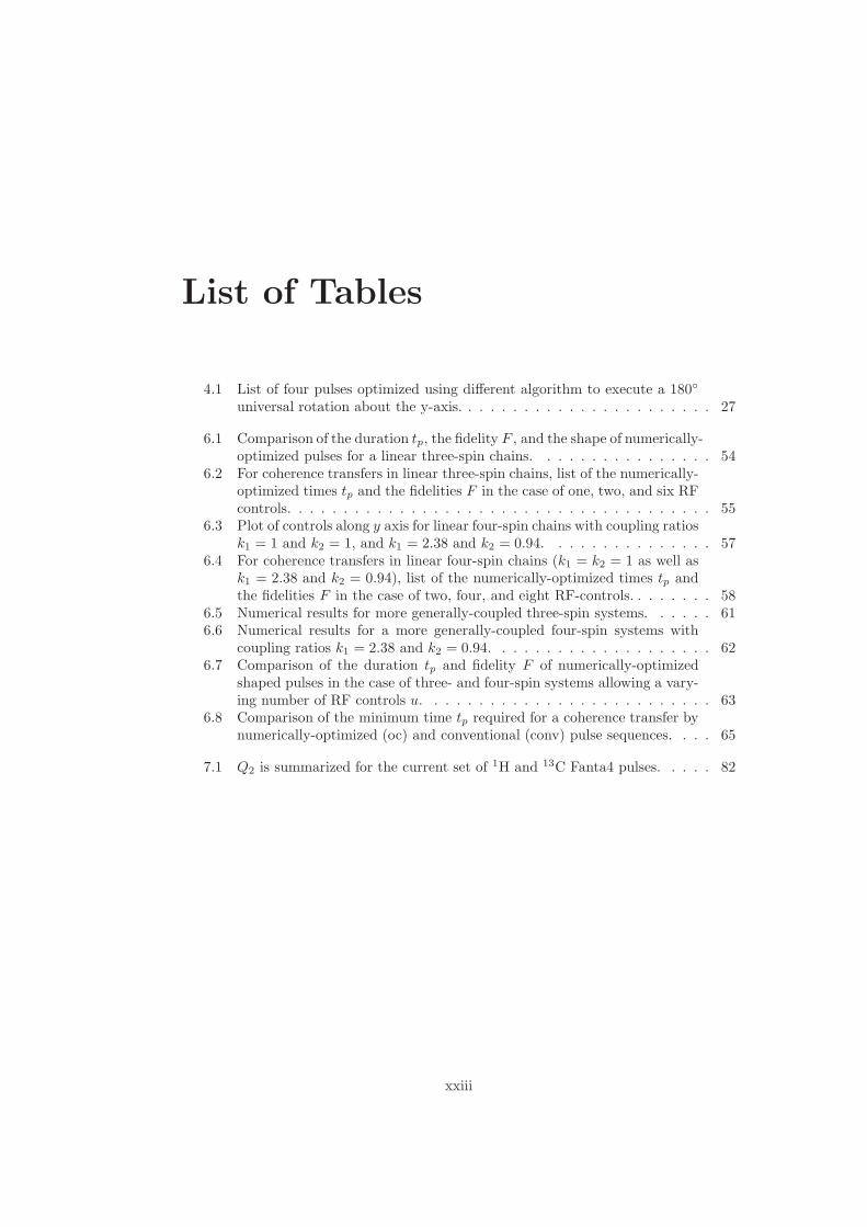
List of Tables
4.1 List of four pulses optimized using different algorithm to execute a 180◦
universal rotation about the y-axis. . . . . . . . . . . . . . . . . . . . . . . 27
6.1 Comparison of the duration tp, the fidelity F , and the shape of numerically-optimized pulses for a linear three-spin chains. . . . . . . . . . . . . . . . 54
6.2 For coherence transfers in linear three-spin chains, list of the numerically-optimized times tp and the fidelities F in the case of one, two, and six RFcontrols. . . . . . . . . . . . . . . . . . . . . . . . . . . . . . . . . . . . . . 55
6.3 Plot of controls along y axis for linear four-spin chains with coupling ratiosk1 = 1 and k2 = 1, and k1 = 2.38 and k2 = 0.94. . . . . . . . . . . . . . . 57
6.4 For coherence transfers in linear four-spin chains (k1 = k2 = 1 as well ask1 = 2.38 and k2 = 0.94), list of the numerically-optimized times tp andthe fidelities F in the case of two, four, and eight RF-controls. . . . . . . . 58
6.5 Numerical results for more generally-coupled three-spin systems. . . . . . 616.6 Numerical results for a more generally-coupled four-spin systems with
coupling ratios k1 = 2.38 and k2 = 0.94. . . . . . . . . . . . . . . . . . . . 626.7 Comparison of the duration tp and fidelity F of numerically-optimized
shaped pulses in the case of three- and four-spin systems allowing a vary-ing number of RF controls u. . . . . . . . . . . . . . . . . . . . . . . . . . 63
6.8 Comparison of the minimum time tp required for a coherence transfer bynumerically-optimized (oc) and conventional (conv) pulse sequences. . . . 65
7.1 Q2 is summarized for the current set of 1H and 13C Fanta4 pulses. . . . . 82
xxiii

xxiv LIST OF TABLES

Chapter 1
Prologue
1.1 Prospect
Nuclear Magnetic Resonance (NMR) is an interesting, important and an indispensabletechnique in a very wide variety of fields. In organic chemistry and structural bio-logy NMR is one of the most important tools for the elucidation and determination ofthree-dimensional structures for small molecules, proteins and other macromolecules. Itgives us information on internal mobility and overall molecular motion in both largeand small molecules. Magnetic Resonance Imaging (MRI) has become one of the bestmethods for obtaining anatomical images of human subjects and animals and for ex-ploring physiological processes. Materials science uses NMR spectroscopy and imagingto describe the structure, motion, and electronic properties of heterogeneous and tech-nologically important substances. NMR is widely used in the food industry to measuremoisture content and to assess the quality of certain foodstuffs. Moreover, NMR is usedto measure the flow of liquids in pipes in industrial processes and to observe the flow ofblood in human beings and is used in the exploration for petroleum.
However, the static magnetic field (B0) and radio frequency (RF) pulses, whichgovern the individual nucleus in a molecule or human tissue during NMR or MRI meas-urements, are associated with intrinsic problems such as inhomogeneous B0 and RFfields delivered to the sample, increase in chemical shift bandwidth due to increase inB0 field strength e.g., for 13C and 31P nuclei, and loss of signal intensity due to relax-ation effects. This thesis focuses on developing, optimizing, and implementing shapedpulses and pulse sequences using principles of optimal control theory which are robustto RF inhomogeneity, large chemical shift bandwidth, and relaxation effects. This helpsto solve some of the most basic yet important problems in NMR spectroscopy and MRimaging.
1.2 Lay out of thesis
Every chapter in general is arranged in the following way,
• Introduction,
• Theory,
• Experiment(s),
1

2 CHAPTER 1. PROLOGUE
• Conclusion
• Appendix (if necessary)
and at the end is a Bibliography of all chapters.
1.3 Synopsis of Chapters
• Chapter 2
Chapter 2 gives the overview of the basic optimal control methodologies, which arealready developed for non-interacting and coupled spin systems. These methodo-logies were used a as basis to develop further control schemes that respects givenconstrains in the rest of the chapters.
• Chapter 3
Using optimal control methods, robust broadband excitation pulses can be de-signed with a defined linear phase dispersion. This makes it possible to createpulses that are equivalent to ideal hard pulses followed by an effective evolutionperiod. For example, in applications, where the excitation pulse is followed bya constant delay, e.g., for the evolution of heteronuclear couplings, part of thepulse duration can be absorbed in existing delays, significantly reducing the timeoverhead of long, highly robust pulses. We refer to the class of such excitationpulses with a defined linear phase dispersion as ICEBERG pulses (Inherent Co-herence Evolution optimized Broadband Excitation Resulting in constant phaseGradients). A systematic study of the dependence of the excitation efficiency onthe phase dispersion of the excitation pulses is presented, which reveals surprisingopportunities for improved pulse sequence performance.
• Chapter 4
Broadband inversion pulses that rotate all magnetization components 180◦ abouta given fixed axis are necessary for refocusing and mixing in high-resolution NMRspectroscopy. The relative merits of various methodologies for generating pulsessuitable for broadband refocusing are considered. The de novo design of 180◦
universal rotation pulses (180◦UR) using optimal control can provide improved per-formance compared to schemes which construct refocusing pulses as compositesof existing pulses. The advantages of broadband universal rotation by optimizedpulses (BURBOP) are most evident for pulse design that includes tolerance to RFinhomogeneity or miscalibration. We present new modifications of the optimalcontrol algorithm that incorporate symmetry principles and relax conservativelimits on peak RF pulse amplitude for short time periods that pose no threat tothe probe. We apply them to generate a set of 180◦BURBOP pulses suitable forwidespread use in 13C spectroscopy on the majority of available probes.
• Chapter 5
Existing optimal control protocols for mitigating the effects of relaxation and/orRF inhomogeneity on broadband pulse performance are extended to the more dif-ficult problem of designing robust, refocused, frequency selective excitation pulses.For the demanding case of short T1 and T2 equal to the pulse length, anticipatedsignal losses can be significantly reduced while achieving nearly ideal frequencyselectivity. Improvements in performance are the result of allowing residual unre-focused magnetization after applying relaxation-compensated selective excitation

1.3. SYNOPSIS OF CHAPTERS 3
by optimized pulses (RC-SEBOP). This unwanted residual signal is easily elim-inated in a single-acquisition sequence or using the two-scan acquisition sequencethat achieves the calculated theoretical performance for the refocused component.
• Chapter 6
We study multiple-spin coherence transfers in linear Ising spin chains with nearestneighbor couplings. These constitute a model for efficient information transfers infuture quantum computing devices and for many multi-dimensional experimentsfor the assignment of complex spectra in nuclear magnetic resonance spectroscopy.We complement prior analytic techniques for multiple-spin coherence transferswith a systematic numerical study where we obtain strong evidence that a certainanalytically-motivated family of restricted controls is sufficient for time-optimality.In the case of a linear three-spin system, additional evidence suggests that prioranalytic pulse sequences using this family of restricted controls are time-optimaleven for arbitrary local controls. In addition, we compare the pulse sequences forlinear Ising spin chains to more realistic spin systems with additional long-rangecouplings between non-adjacent spins. We implement the derived pulse sequencesin three and four spin systems and demonstrate that they are applicable in real-istic settings under relaxation and experimental imperfections—in particular—byderiving broadband pulse sequences which are robust with respect to frequencyoffsets.
• Chapter 7
We present “Fantastic Four” (Fanta4: Flavored rf and offset robust Alike-durationNumerically-optimized Trouble-free Applicable 4) pulses, a set of highly robust,optimal control-based shaped pulses that are able to replace all hard pulses, in aone-to-one fashion, in pulse sequences consisting of 90◦ and 180◦ pulses for betterperformance. The set of four pulses for each nucleus consists of point-to-point(PP) 90◦ and 180◦, and universal rotation (UR) 90◦ and 180◦ pulses of identicalduration (1 ms). These pulses are robust to a range of frequency offsets (20 kHzfor 1H and 35 kHz for 13C) and tolerate reasonably large radio frequency (RF)inhomogeneity/miscalibration (±15% for 1H and ±10% for 13C). We compare theexperimental performance of conventional pulse sequences to the correspondingFanta4-pulse sequence.

4 CHAPTER 1. PROLOGUE

Chapter 2
Optimal control methodologies
2.1 Introduction
Optimal control theory originally was introduced for optimizations in engineering andeconomy. In recent years, optimal control theory is considered as a methodology for pulsesequence design in liquid state NMR, solid state NMR, EPR, DNP, quantum computing,and being used in MR imagining [1]. It provides systematically imposing desirableconstraints on a spin system evolution and therefor has a wealth of applications. Inapplications of NMR spectroscopy and MRI, it is desirable to have optimized pulses andpulse sequences tailored to specific applications, such as, pulses which are robust to radiofrequency (RF) miscalibration/inhomogeneity, which excites spins at large chemical shiftranges and robust to relaxation effects of the individual nucleus. It helps to maximizethe coherence transfer between coupled spins in multi-dimensional NMR pulse sequencesand improves the overall signal to noise ratio.
From an engineering perspective all these problems are challenges in optimal controlwhere one is interested in tailoring the excitation of a dynamical system to maximizea given performance criterion. This chapter introduces a basic overview of the use ofprinciples of optimal control theory to develop algorithms to design robust broadbandexcitation pulses (Chapter 3), universal rotation pulses (Chapter 4), relaxation and RFinhomogeneity optimized selective excitation pulses (Chapter 5), and pulses for effectivemultiple coherence transfer for more than two spin system (Chapter 6).
2.2 Optimal control using Bloch equation
In 1946 Felix Bloch formulated a set of equations that describe the behavior of a non-interacting nuclear spins in a magnetic field under the influence of RF pulses. Blochassumed that nuclear spins relax following the application of RF pulses along z-axisand in the x-y plane at different rates following a first -order kinetics. These ratesare designated 1/T1 and 1/T2 for z-axis and x-y plane, respectively. T1 is called spin-lattice (longitudinal) relaxation and T2 is called spin-spin (transverse) relaxation. Inthe following, we will use Bloch equations without and with relaxation to calculate thetrajectories of the non-interacting spins.
5
6 CHAPTER 2. OPTIMAL CONTROL METHODOLOGIES
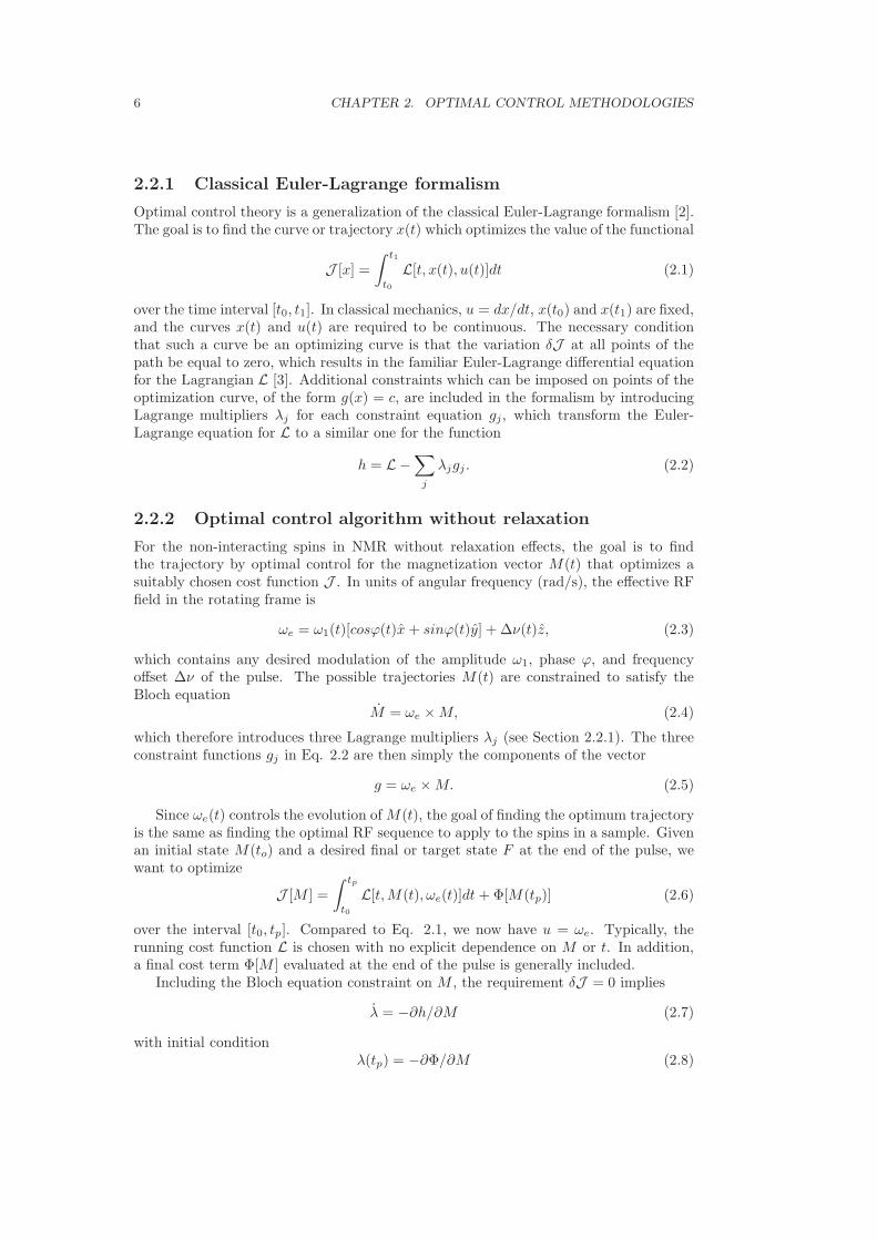
2.2.1 Classical Euler-Lagrange formalism
Optimal control theory is a generalization of the classical Euler-Lagrange formalism [2].The goal is to find the curve or trajectory x(t) which optimizes the value of the functional
J [x] =
∫ t1
t0
L[t, x(t), u(t)]dt (2.1)
over the time interval [t0, t1]. In classical mechanics, u = dx/dt, x(t0) and x(t1) are fixed,and the curves x(t) and u(t) are required to be continuous. The necessary conditionthat such a curve be an optimizing curve is that the variation δJ at all points of thepath be equal to zero, which results in the familiar Euler-Lagrange differential equationfor the Lagrangian L [3]. Additional constraints which can be imposed on points of theoptimization curve, of the form g(x) = c, are included in the formalism by introducingLagrange multipliers λj for each constraint equation gj, which transform the Euler-Lagrange equation for L to a similar one for the function
h = L −∑
j
λjgj . (2.2)
2.2.2 Optimal control algorithm without relaxation
For the non-interacting spins in NMR without relaxation effects, the goal is to findthe trajectory by optimal control for the magnetization vector M(t) that optimizes asuitably chosen cost function J . In units of angular frequency (rad/s), the effective RFfield in the rotating frame is
ωe = ω1(t)[cosϕ(t)x + sinϕ(t)y] + ∆ν(t)z, (2.3)
which contains any desired modulation of the amplitude ω1, phase ϕ, and frequencyoffset ∆ν of the pulse. The possible trajectories M(t) are constrained to satisfy theBloch equation
M = ωe ×M, (2.4)
which therefore introduces three Lagrange multipliers λj (see Section 2.2.1). The threeconstraint functions gj in Eq. 2.2 are then simply the components of the vector
g = ωe ×M. (2.5)
Since ωe(t) controls the evolution of M(t), the goal of finding the optimum trajectoryis the same as finding the optimal RF sequence to apply to the spins in a sample. Givenan initial state M(to) and a desired final or target state F at the end of the pulse, wewant to optimize
J [M ] =
∫ tp
t0
L[t,M(t), ωe(t)]dt +Φ[M(tp)] (2.6)
over the interval [t0, tp]. Compared to Eq. 2.1, we now have u = ωe. Typically, therunning cost function L is chosen with no explicit dependence on M or t. In addition,a final cost term Φ[M ] evaluated at the end of the pulse is generally included.
Including the Bloch equation constraint on M , the requirement δJ = 0 implies
λ = −∂h/∂M (2.7)
with initial conditionλ(tp) = −∂Φ/∂M (2.8)

2.2. OPTIMAL CONTROL USING BLOCH EQUATION 7
for the time evolution of λ, and
∂h(t)/∂ωe(t) = 0, (2.9)
at all points on the optimal trajectory, which provides a means for adjusting the RFcontrols. By analogy with the Hamiltonian formalism of classical mechanics, M and λare conjugate variables, since
M = ωe ×M = ∂h/∂λ. (2.10)
according to Eqs. 2.2 and 2.5.
2.2.3 Optimal control algorithm with relaxation
Following section 2.2.2, the Bloch equation for the non-interacting spins with relaxationT1 and T2 will be
M(t) = ωe(t)×M(t) +D[M0 −M(t)], (2.11)
where M0 = z is the unit equilibrium polarization for appropriately normalized units,the effective field ωe in rad/s is given in terms of the time-dependent RF amplitude ω1
and phase ϕ in Eq. 2.3 and the relaxation matrix is
D =
1/T2 0 00 1/T2 00 0 1/T1
. (2.12)
Including relaxation a time-dependent hamiltonian h can be redefined in terms of aLagrange multiplier λ as
h(t) = λ(t) · M(t) = λ · [ωe ×M +D(M0 −M)], (2.13)
which returns the Bloch equation as
M = ∂h/∂λ, (2.14)
with the known value M(t0) at the beginning of the pulse. For a given cost functionΦ chosen to measure the pulse performance, the optimization formalism results in theconjugate or adjoint equation
λ(t) = −∂h/∂M (2.15)
λ(t) = ωe(t)× λ(t) +Dλ(t), (2.16)
with the value λ(tp) = ∂Φ/∂M required at the end of the pulse, giving λ(tp) = F forthe cost
Φ = M(tp) · F, (2.17)
for example.The final necessary condition that must be satisfied by a pulse that optimizes the
cost function is∂h(t)/∂ωe(t) = 0 = M(t)× λ(t), (2.18)
at each time. For a non-optimal pulse, Eq. 2.18 is not fulfilled . It then represents agradient giving the proportional adjustment to make in the controls ωe(t) for the nextiteration towards an optional solution. For more details and applications refer to Ref. [4]and Chapter 5.
This numerical algorithm can be generalized for desired applications in NMR such asexcitation and inversion of a given spin system with defined constraints. The followingsteps explain how the optimizing the cost (Φ) /desired target (F ) can be incorporatedin an algorithm:

8 CHAPTER 2. OPTIMAL CONTROL METHODOLOGIES
1. Choose initial RF controls/sequence ω0e.
2. Evolve M forward in time from the initial state M(t0).
3. Evolve λ backwards in time from the target state F (see Figure 2.1).
4. ωk+1e (t) → ωk
e(t) + ǫ[M(t)× λ(t)], where ǫ is a suitable step size.
5. With these as the new controls, go to step 2 until a desired convergence of Φ isreached.
More details can be found in Ref [5].
t0 tp
M( )t0
M( )t
l( ) = Ftpl( )t
M ( )opt t l ( )opt t<=>
t
Figure 2.1: (Figure adapted from Ref. [5]) Optimization scheme. For a given RF sequence ωe(t), theinitial state M(t0) evolves to some final state M(tp) through a sequence of intermediate states, shownschematically as the solid line connecting M(t0) and M(tp). Similarly, the desired final target state F ,which equal to the Lagrange multiplier term λ(tp) according to Eqs. 2.8 and 2.17, evolves backwards intime to some initial state λ(t0). The separate paths for M(t) and λ(t) becomes equal for the optimizedRF sequence ωopt(t) and drives M(t0) to λ(tp) = F . At each time, a comparison of the two paths viaM(t) × λ(t) gives the proportional adjustment ǫ to make in each component of the control field ωe(t)to bring the two paths closer together.
2.3 Optimal control using Liouville-von Neuman equa-tion
The Bloch equation is unable to treat coupled spin systems and hence we have to changeto Liouville-von Neuman equation where the state of the spin system is defined bythe density operator ρ(t). The Liouville-von Neuman equation for transfer betweenHermitian operators in absence of relaxation is
ρ(t) = −i[(H0 +
m∑
k=1
uk(t)Hk), ρ(t)], (2.19)
where H0 is the free evolution Hamiltonian, Hk are the RF Hamiltonians correspond-ing to available control fields and u(t) = (u1(t), u2(t), ..., um(t)) represents the vector ofamplitudes that can be changed and which is referred to as control vector. The prob-lem is to find the optimal control amplitudes uk(t) of the RF fields that steer a giveninitial density operator ρ(0) = ρ0 in a specified time T to a density operator ρ(T ) with

2.3. OPTIMAL CONTROL USING LIOUVILLE-VON NEUMAN EQUATION 9
maximum overlap to some desired target operator F . For Hermitian operator ρ0 and F ,this overlap can be measured by the standard inner product
〈F |ρ(T )〉 = Tr{F † ρ(T )}. (2.20)
Hence, the performance index Φ of the transfer process can be defined as
Φ = 〈F |ρ(T )〉. (2.21)
In the following, we will assume for simplicity that the chosen transfer time T is discret-ized in N equal steps of duration ∆t = T/N and during each step, the control amplitudesuk are constant, i.e. during the jth step the amplitude uk(t) of the kth control Hamilto-nian is given by uk(j). The time-evolution of the spin system during a time step j isgiven by the propagator
Uj = exp{−i∆t(H0 +
m∑
k=1
uk(t)Hk)}. (2.22)
The final density operator at time t = T is
ρ(T ) = Un....U1ρ0U†1 ....U
†N , (2.23)
and the performance function Φ to be maximized can be expressed as
Φ = 〈F |Un....U1ρ0U†1 ....U
†N 〉. (2.24)
Using the definition of the inner product (Eq. 2.21) and the fact that the trace of aproduct is invariant under cyclic permutations of the factors, this can be rewritten as
Φ = 〈U †j+1....U
†NFUN ....Uj+1
︸ ︷︷ ︸
λi
|Uj ....U1ρ0U†1 ....U
†j
︸ ︷︷ ︸
ρj
〉. (2.25)
where ρj is the density operator ρ(t) at time t = j∆t and λj is the backward propagatedtarget operator F at the same time t = j∆t. Let us see how the performance Φ changeswhen we perturb the control amplitude uk(j) at time step j to uk(j) + δ uk(j). FromEq. 2.22, the change in Uj to first order in δ uk(j) is given by
δUj = −i∆tδuk(j)HkUj (2.26)
with
Hk∆t =
∫ ∆t
0
Uj(τ)HkUj(−τ)dτ (2.27)
and
Uj(τ) = exp{− iτ
(H0 +
m∑
k=1
uk(j)Hk
)}. (2.28)
This follows from the standard formula
d
dxeA+xB|x=0 = eA
∫ 1
0
eAτBe−Aτdτ. (2.29)
For small ∆t (when ∆t ≪‖ H0 +∑m
k=1 uk(j)Hk ‖ −1), Hk ≈ Hk and using Eqs. 2.25and 2.26 we find to first order in ∆t

10 CHAPTER 2. OPTIMAL CONTROL METHODOLOGIES
Gj =δΦ
δuk(j)= −〈λj |i∆t[Hk, ρj ]〉. (2.30)
Observe we increase the performance function Φ if we choose
uk(j) → uk(j) + ǫδΦ
δuk(j), (2.31)
where ǫ is a small step size. This forms the basis of the following algorithm, which isknown as the gradient ascent pulse engineering (GRAPE) to distinguish it from conven-tional gradient approaches used in NMR based on difference methods.
Basic GRAPE algorithm
1. Guess initial controls uk(j).
2. Starting from ρ0, calculate ρj = Uj ...U1ρoU†1 ...U
†j for all j ≤ N .
3. Starting from λN = F , calculate λj = U †j+1...U
†NFUN ...Uj+1 for all j ≤ N .
4. Evaluate δΦδuk(j)
and update the m x N control amplitudes uk(j) according to
Eq.2.31.
5. With these as the new controls, go to step 2.
The algorithm is terminated if the change in the performance index Φ is smaller thana chosen threshold value.
For treatment of non-Hermitian operators and for relaxation-optimized coherencetransfer refer to Refs. [6, 7].

Chapter 3
Linear phase slope in pulsedesign: Application tocoherence transfer
3.1 Introduction
This chapter is a part of an article [8] and it focuses on applications and experimentalimplementations of ICEBERG ( Inherent Coherence Evolution optimized BroadbandExcitation Resulting in constant phase Gradients) pulses. The fundamental goal ofpulse sequence design is to control spin trajectories. Although the ideal final state of thesample magnetization just prior to acquisition may be obvious for a given application,how to achieve this state can be less obvious. Optimal control theory [9] is a powerfulmethod which can be applied to this problem. It has been used, for example, to deriveultra-broadband excitation pulses, BEBOP [10–14], which are tolerant to RF inhomo-geneity/ miscalibration and require no phase correction. This imposes a rather stringentrequirement on the optimal control algorithm for a range of possible RF calibrations, itmust drive all spins within the desired range of resonance offsets to the same final state.Yet, a linear phase dispersion in the final magnetization as a function of offset is readilycorrected in many practical applications utilizing, for example, hard pulses or Gaussianpulses [15].
We have formerly compared BEBOP performance (no phase correction required)to a phase-corrected hard pulse, since this is an excellent benchmark for broadbandexcitation. BEBOP pulses are exceptional by this standard, but a fairer comparisonwould entail optimized pulses that can be phase-corrected, also. We therefore considerthe advantages of allowing this increased flexibility in pulse design.
The slope of the phase as a function of offset appears to be an important parameterfor pulse design. Applications include increased bandwidth for a given pulse lengthcompared to equivalent pulses requiring no phase correction (or, shorter pulses for thesame bandwidth), selective pulses, and pulses that mitigate the effects of relaxation [16].In particular, we consider pulses for coherence transfer that make it possible to absorbsome of the evolution time for heteronuclear couplings into the excitation pulse. Onecan then utilize specific performance benefits of relatively long pulses without addingsignificantly to the experiment time.
11
12 CHAPTER 3. LINEAR PHASE SLOPE IN PULSE DESIGN
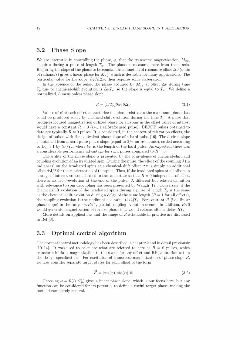
3.2 Phase Slope
We are interested in controlling the phase, ϕ, that the transverse magnetization, Mxy,acquires during a pulse of length Tp. The phase is measured here from the x-axis.Requiring the slope of the phase to be constant as a function of resonance offset ∆ν (unitsof radians/s) gives a linear phase for Mxy, which is desirable for many applications. Theparticular value for the slope, ∂ϕ/∂∆ν, then requires some elaboration.
In the absence of the pulse, the phase acquired by Mxy at offset ∆ν during timeTp due to chemical-shift evolution is ∆νTp, so the slope is equal to Tp. We define anormalized, dimensionless phase slope
R = (1/Tp)∂ϕ/∂∆ν (3.1)
Values of R at each offset characterize the phase relative to the maximum phase thatcould be produced solely by chemical-shift evolution during the time Tp. A pulse thatproduces focused magnetization of fixed phase for all spins in the offset range of interestwould have a constant R = 0 (i.e., a self-refocused pulse). BEBOP pulses obtained todate are typically R ≈ 0 pulses. It is considered, in the context of relaxation effects, thedesign of pulses with the equivalent phase slope of a hard pulse [16]. The desired slopeis obtained from a hard pulse phase slope (equal to 2/π on resonance), scaled accordingto Eq. 3.1 by t90/Tp, where t90 is the length of the hard pulse. As expected, there wasa considerable performance advantage for such pulses compared to R = 0.
The utility of the phase slope is presented by the equivalence of chemical-shift andcoupling evolution of an irradiated spin. During the pulse, the effect of the coupling J (inradians/s) on the irradiated spins at a chemical-shift offset ∆ν is simply an additionaloffset ±J/2 for the ± orientation of the spins. Thus, if the irradiated spins at all offsets ina range of interest are transformed to the same state so that R = 0 independent of offset,there is no net J-evolution at the end of the pulse. A different but related definitionwith relevance to spin decoupling has been presented by Waugh [17]. Conversely, if thechemicalshift evolution of the irradiated spins during a pulse of length Tp is the sameas the chemical-shift evolution during a delay of the same length (R = 1 for all offsets),the coupling evolution is the undiminished value (J/2)Tp. For constant R (i.e., linearphase slope) in the range 0<R<1, partial coupling evolution occurs. In addition, R<0would generate magnetization of reverse phase that would refocus after a delay RTp.
More details on applications and the range of R attainable in practice are discussedin Ref [8].
3.3 Optimal control algorithm
The optimal control methodology has been described in chapter 2 and in detail previously[10–14]. It was used to calculate what are referred to here as R = 0 pulses, whichtransform initial z magnetization to the x-axis for any offset and RF calibration withinthe design specifications. For excitation of transverse magnetization of phase slope R,we now consider separate target states for each offset of the form
−→F = [cos(ϕ), sin(ϕ), 0] (3.2)
Choosing ϕ = R(∆νTp) gives a linear phase slope, which is our focus here, but anyfunction can be considered for its potential to define a useful target phase, making themethod completely general.
3.4. APPLICATIONS 13
We have previously input random noise for the initial RF used to start the algorithm.Characterizing the performance of various modifications and additions to the algorithmwas an important goal, and we wanted to avoid imposing any bias on what mightconstitute the best final solution. Inputting noise also served to demonstrate the powerand efficiency of optimal control, showing that it is not necessary to guess an approximatesolution in order for the algorithm to either converge or converge in a useable timeframe, which is often the case in standard optimization routines. Some of the resultingpulses look very much like noise themselves, although their outstanding performancedemonstrates they are not at all random.
Now that the algorithm is well-established, we turn to the derivation of smooth pulseshapes. We start the algorithm with an initial RF pulse of constant small amplitude(approximately zero) and constant phase (π/4). This results in a class of sinc-like pulseshapes that is reminiscent of, and appears to include, polychromatic pulses [18] as asubset. In addition to being easy to implement on a wide range of spectrometers, theshape of the new pulses depends in a very regular fashion on R for values in the range0 ≤ R ≤ 1.
3.4 Applications
3.4.1 Shorter broadband excitation
A hard pulse excites transverse magnetization Mxy with an approximately linear phaseslope (R = 2/π on resonance) that can be corrected in many useful applications. Al-though a hard pulse is probably the workhorse of NMR spectroscopy, the excitationprofile is not uniform as a function of resonance offset, nor is the phase slope. At fieldstrengths approaching 1 GHz and typical 13C probe limits on peak RF amplitude of∼15 kHz (Tp = 16.7 µs), there is room for improvement, as shown in Fig. 3.1. Anideally calibrated pulse excites 95% of the attainable transverse magnetization over anoffset range of ±17 kHz, and excites less than 90% over ±25 kHz. The phase is linear towithin ±2◦ over the entire offset range of 50 kHz, but can be 3◦ − 4◦ over large parts ofthe spectrum, depending on RF inhomogeneity or miscalibration. Accumulated signallosses can be significant when large pulse trains are applied.
Previously, we derived a relatively short 125 µs pulse requiring no phase correction(R = 0) that uniformly excites 99% magnetization over 50 kHz bandwidth with toleranceto RF inhomogeneity of ±10% [13]. If the pulse is no longer required to be self-refocused,we find the 39 µs, R = 1/2 pulse shown in Fig. 3.2. The excited Mxy is greater than 0.99over the entire 50 kHz bandwidth used in the optimization, and also provides toleranceto RF miscalibration of ±7% (> 98% for ±10% miscalibration). Deviations in phaselinearity (absolute value) are less than 1◦ over most of the optimization window of ±25kHz offset and ±10% RF inhomogeneity, rising to 3◦ − 4◦ only at the extreme edges ofthe window.
3.4.2 Coherence transfer
Consider the basic element of a coherence transfer experiment shown in Fig. 3.3A, a 90◦
pulse followed by a delay of length τ .
For a pulse that produces a linear phase slope in the transverse magnetization, theparameter R can be interpreted as the fraction of the pulse length in which the netchemical-shift (or coupling) evolution occurs, as discussed in Section 3.2. Hence, a pulse

14 CHAPTER 3. LINEAR PHASE SLOPE IN PULSE DESIGN
0.9
0.9
0.9
0.9
0.95
0.95
0.95
0.95
0.95
0.95
0.98
0.98
0.98
0.98
0.98
0.98
0.99
0.99
0.99
0.99
0.99
0.99
B1/B
10
Offset [kHz]−20 −10 0 10 20
0.9
0.95
1
1.05
1.1
1
1
11
1
1
11
1
1
1
1
2
2
2
2
2
2
2
2
2
2
3
3
3
3
3
3
4
4
4
4
Offset [kHz]−20 −10 0 10 20
Mxy
Phase deviation
Figure 3.1: (Color online) Performance of a 16.7 µs hard pulse, peak RF amplitude = 15 kHz.Transverse magnetization Mxy (left panel) and absolute value of the phase deviation from linearity(right panel) are plotted as functions of resonance offset and RF miscalibration/inhomogeneity B1/B◦
1.
B1 is the variable RF amplitude and B◦
1is the nominal RF amplitude.
of phase slope R and duration Tp produces the same phase evolution that would occurfor transverse magnetization during a time-delay interval
Tevol = RTp, (3.3)
as illustrated in Fig. 3.3B. The remaining fraction of the pulse can be represented by a90◦ excitation pulse of length
Texc = Tp − Tevol = (1 −R)Tp, (3.4)
in which no phase evolution occurs. Thus, the total time for the 90◦ − τ element ofthe sequence can be reduced by the time Tevol. The performance advantages of certainkinds of longer pulses, such as BEBOP or selective pulses, can then be more fullyexploited if they are designed with large R to avoid increasing the experiment time toan unsatisfactory degree. This interpretation of R also provides additional insight intorelaxation-compensated pulses, which can be idealized as excitation with no relaxationduring Texc followed by chemical-shift evolution and relaxation during Tevol [8].
3.4.3 Experimental
Comparison with hard pulse
Figure 3.4 shows the amplitude and phase of ICEBERG pulses with R from -0.5 to 0.95and Figure 3.5 shows their excitation profile compared to hard pulse. All experimentswere implemented on a Bruker 200 MHz AVANCE spectrometer equipped with SGUunits for RF control and linearized amplifiers, utilizing a double-resonance 5 mm SEIprobehead and gradients along the z-axis. Measurements are the residual HDO signal ina sample of 99.96% D2O doped with CuSO4 to a T1 relaxation time of 280 ms at 298◦K.Signals were obtained at offsets between −25 kHz to 25 kHz in steps of 100 Hz. To

3.5. CONCLUSION 15
0.990.99
0.99
0.99
0.99
B1 /
B10
Offset [kHz]
B1 /
B10
B1 /
B10
B1 /
B10
B1 /
B10
−20 −10 0 10 200.9
0.95
1
1.05
1.1
1
1 1
12
2 2
2
3
3 3
3
Offset [kHz]
−20 −10 0 10 20.9
.95
1
1.05
1.1
0 10 20 30−15
−10
−5
0
5
10
15
B1 [
kHz]
Time [ µs]
Phase Deviation [deg]MxyRF Pulse
Figure 3.2: (Color online) Amplitude-modulated pulse of length 39 µs and peak RF amplitude = 15kHz, optimized to excite transverse magnetization Mxy with linear phase slope R = 1/2 over resonanceoffsets of 50 kHz. The pulse serendipitously provides significant tolerance to RF miscalibration B1/B◦
1
with small phase deviations (absolute value) from linearity, as shown in the middle and right panels.The 50 kHz, ±10% RF miscalibration window used for the simulations shows Mxy>0.99 and phasedeviations less than 1◦ over most of these ranges, with deviations of 3◦ at the extreme offsets andmiscalibrations at the corners of the window.
reduce the effects of RF field inhomogeneity within the coil itself, approximately 40 µlof the sample solution was placed in a 5 mm Shigemi limited volume tube.
Coherence transfer in HMQC
The viability of employing relatively long ICEBERG pulses with improved excitationprofile compared to a hard pulse is illustrated in Figure 3.7, using a 13C excited anddetected HMQC experiment as an example (Fig. 3.6). Although this experiment wouldrealistically be performed using 1H excitation and detection, the large 13C chemicalshift serves as a proxy for similar correlation experiments based on 19F or 31P excitationwhich will benefit from the ICEBERG scheme.
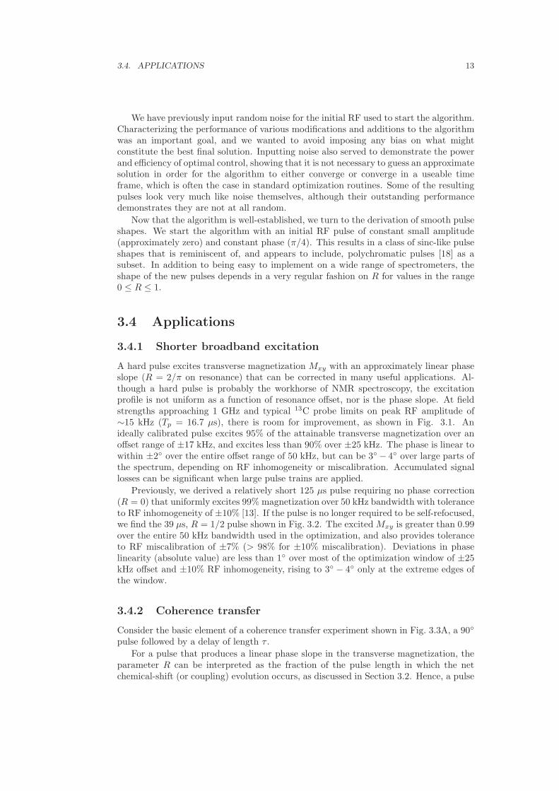
HMQC performance using a 1.428 ms ICEBERG pulse (R = 0.95), optimized toachieve uniform excitation over the full carbon chemical- shift range, is compared to thesame experiment using a 35.7 µs hard pulse (i.e., RF amplitude equal to the peak RFof the ICEBERG pulse). Embedding the ICEBERG pulse in the delay period resultsin an effective excitation pulse length Texc = 71.4 µs, according to Eq. 3.4. Thus, theduration of the entire experiment is practically identical in both cases. However, incontrast to the ICEBERG version, which provides uniform excitation across the entireoffset range, signal intensity in the hard pulse version is reduced by as much as 38% atthe edges of the carbon chemical-shift range. Further details are provided in Figure 3.7.The experiments were recorded on a Bruker AVANCE 750 MHz spectrometer using atriple resonance inverse detection room temperature probe head. 1024×128 data pointswere acquired with corresponding spectral widths of 200.8 ppm (13C) and 8.5 ppm (1H).Sixteen transients per increment gave an overall experiment time of 35 min for each ofthe two experiments.
3.5 Conclusion
The features of pulses which excite transverse magnetization with linear phase as afunction of offset have been presented. A pulse with phase slope R at resonance offset

16 CHAPTER 3. LINEAR PHASE SLOPE IN PULSE DESIGN
90o
90o
Tp
Texc Tevol
0 time
t
A
B
Figure 3.3: The use of a linear phase slope pulse to reduce the delay τ in selective coherence transferin the case where Tp is relatively long. (A) R = 0, requiring τ = 1/(2J). (B) R ≥ 0, with Tevol = RTp
resulting in chemical shift evolution ∆νTevol during the pulse and thus a coupling evolution (J/2)Tevol ,reducing the delay correspondingly. The pulse can be represented by excitation with no phase evolutionduring the time Texc followed by free precession during Tevol.
∆ν produces a net chemical-shift evolution R∆νTp during a pulse of length Tp. Thelinear phase evolution gives a J-coupling of RJ during the pulse. Large R then results insignificant coupling evolution during the pulse, enabling the use of what might otherwisebe prohibitively long pulses for coherence transfer.

3.5. CONCLUSION 17
0.95
0.75
0.5
0.25
0
-0.5
R Shaped pulse
Figure 3.4: The RF amplitude and Phase are plotted as a function of time for a series of 1 ms pulsesdesigned using different values of R and with RFlim of 10 kHz to excite a bandwidth of ∆ν = 50 kHz.

18 CHAPTER 3. LINEAR PHASE SLOPE IN PULSE DESIGN
-25 0 25
Dn ( )kHz
0.95
0.75
0.5
0.25
0
-0.5
R Excitation Profile
Square pulse: 0 and 1 order phase correctionst
Square pulse: with linear phase
0
2/p
Figure 3.5: Excitation profile of ICEBERG pulses with different R (Fig. 3.4) compared with hardpulse (Tp = 16.7 µs).

3.5. CONCLUSION 19
1H
13C
a
b
1H
13C
D
d DEC
DEC
d
d d
D
D
D
f1 f1 f2 f2
f1 f1 f2 f2
t1
t1
frec
frec
ICEBERG
D*
Figure 3.6: Carbon excited and detected HMQC experiment using a conventional 90◦ hard pulse(a) and an ICEBERG pulse for excitation (b). Filled rectangles correspond to 90◦ pulses while openrectangles indicate 180◦ pulses, with the wide box on 13C representing a refocussing pulse constructedout of two phase-modulated excitation pulses [14] using the principle described in Ref. [19]. Phases arex with the exception of φ1 = x, -x; φ2 = x, x, -x, -x; and φrec = x, -x, -x, x. Delays are ∆ = 1/(21JCH ),with ∆∗ reduced by the effective evolution period of the ICEBERG pulse, R·Tp. Both experiments havepractically identical overall sequence lengths but the offset-compensated ICEBERG HMQC provideshigher sensitivity especially at the edges of the carbon chemical shift range.
20 CHAPTER 3. LINEAR PHASE SLOPE IN PULSE DESIGN
a
100110 ppm 100110 ppm 20 10 5 ppm 20 10 ppm
b c
ppmd( C)13
ppm
d( H)1
hard
ICEBERG
160 120 80 40
2
4
6
8
0.0 -5.05.0 -10.010.0
Offset [kHz]
0.6
0.8
1.0
15.0 -15.0
d
Figure 3.7: (Color online) Experimental data acquired on hydroquinidine in CDCl3 are shown in (a),with the ICEBERG-HMQC cross peaks shown in black and the hard pulse version shown in gray witha slight shift in 1H. Slices of the encircled cross peaks near δ(13C)= 100 ppm are compared in (b) forICEBERG (left) and the hard-pulse version (right). A similar comparison showing the loss off signal inthe hard-pulse version is shown in (c) near δ(13C)= 12 ppm. The experiment was implemented usinga 1.428 ms ICEBERG pulse (R = 0.95, giving an effective contribution to the overall pulse sequencelength of 1.428 ms× 0.05 = 71.4 µs) and a hard pulse of 35.7 µs duration. The simulation of the offsetprofiles of the ICEBERG (dash-dotted line) and hard 90◦ pulse (solid line) are shown in (d) togetherwith the experimental signal intensities (ICEBERG-HMQC signal intensities normalized to 1.0).

Chapter 4
Broadband 180◦ universalrotation pulses
4.1 Introduction
This chapter is a part of an article [20] and it focuses on applications, and experimentalimplementation and comparison of BURBOP pulses with Chirp80 [21]. Many NMR ap-plications require refocusing of transverse magnetization, which is easily accomplished onresonance by any good inversion pulse sandwiched between delays, i.e., the standard ∆–180◦–∆ block. For broadband applications, a universal rotation (UR) pulse that rotatesany orientation of the initial magnetization 180◦ about a given fixed axis is required torefocus all transverse magnetization components. A simple hard pulse functions as a URpulse only over a limited range of resonance offsets that cannot be increased significantlydue to pulse power constraints.
Although a great deal of effort has been devoted to increasing the bandwidth ofinversion pulses, most broadband inversion pulses [22–37] execute only a point-to-point(PP) rotation for one specific initial state, magnetization Mz → −Mz, and are not URpulses. However, two PP inversion pulses with suitable inter-pulse delays can be used toconstruct a refocusing sequence [38,39], which is effectively a 360◦UR pulse. Alternatively,a 180◦UR refocusing pulse can be constructed from three adiabatic inversion pulses [40]with either pulse length or bandwidth of the adiabatic frequency sweep in the ratio 1:2:1.More generally, we have shown that one can construct a UR pulse of any flip angle froma PP pulse of half the flip angle preceded by its time- and phase-reversed waveform [41].Thus, a 180◦UR pulse can be constructed from two 90◦PP pulses.
The reliance on composites of PP pulses to construct UR pulses highlights the per-ceived difficulty of creating stand-alone UR pulses. The de novo design of UR pulses forNMR spectroscopy has received comparatively little attention [30, 42], so it is an openquestion whether the composite constructions using PP pulses achieve the best possibleperformance. Yet, the demonstrated capabilities of optimal control for designing PPpulses [43–56] are equally applicable to the design of UR pulses [57–59]. The requiredmodifications to the basic optimal control algorithm are fairly straightforward [57,60,61]and maintain the same flexibility for incorporating tolerance to variations in experiment-ally important parameters, such as RF homogeneity or relaxation.
In this chapter, we design broadband refocusing pulses by optimizing the propagatorfor the required UR transformation. We introduce new optimal control strategies tailoredto take advantage of specific opportunities available in the design of UR pulses. The
21

22 CHAPTER 4. BROADBAND 180◦ UNIVERSAL ROTATION PULSES
culmination of these efforts is a set of low-power, high-performance broadband refocusingpulses that satisfy the power constraints of widely available probeheads and complexmultipulse sequences.
4.2 Optimal control algorithm for 180◦UR pulses
A general procedure for creating a desired unitary propagator in an arbitrary (closed)quantum system is given in [57, 60–62]. Time evolution proceeds according to a matrixexponential of the system Hamiltonian. For two-level systems, as in many NMR applic-ations involving a single noninteracting spin-1/2 species, this evolution is well-known tobe equivalent to a rotation of the 3D vector representing the state of the system aboutthe effective applied field [63]. The relatively abstract general procedure for propagatoroptimization can be made considerably more transparent in this case.
4.2.1 Flavor I (basic vanilla)
The algorithm for generating UR pulses in the single-spin case is a straightforwardmodification of the PP algorithm. A 180◦UR pulse applied, for example, along the y-axis to magnetization M effects the transformation (Mx,My,Mz) → (−Mx,My,−Mz).This is simply three separate PP transformations of the initial states M1 = (1, 0, 0),M2 = (0, 1, 0), M3 = (0, 0, 1) to their respective target states F 1 = (−1, 0, 0), F 2 =(0, 1, 0), F 3 = (0, 0,−1). The cost function comparing the final states Mkf (k = 1, 2, 3)at the end of an RF pulse to the target states is
Φ = F 1 ·M 1f + F 2 ·M2f + F 3 ·M3f . (4.1)
The algorithm proceeds in the standard fashion using this cost function. We will referto this as algorithm A.
This simple intuitive modification to the cost is exactly equivalent to an analogousprocedure given in [57] for optimizing the unitary propagator, which can be seen asfollows. The rotation operator RF in 3D corresponding to the target propagator thatgenerates a 180◦ rotation about the y-axis is given by
RF =
−1 0 00 1 00 0 −1
=
......
...F 1 F 2 F 3
......
...
, (4.2)
i.e., the i th column is the corresponding PP target F i.The actual rotation operator at the end of a pulse of length Tp is
R(Tp) = R(Tp)
1 0 00 1 00 0 1
= R(Tp)
......
...M 1 M2 M 3
......
...
=
......
...M 1f M2f M 3f
......
...
, (4.3)

4.3. BURBOP COMPARED TO REFOCUSING WITH PP PULSES 23
with the rotation transforming each column to its associated final state for the individualPP transformations.
The cost is again given by the projection of the final state onto the target state, withthe inner product
ΦR = 〈RF |R(Tp) 〉 = Tr [RTF R(Tp)], (4.4)
where superscript T denotes the transpose, and the operator Tr returns the trace (sumof diagonal elements) of its argument. We then have
RTF R(Tp) =
· · ·F 1 · · ·· · ·F 2 · · ·· · ·F 3 · · ·
......
...M1f M2f M3f
......
...
. (4.5)
The sum over diagonal elements of this matrix product gives Eq. [ 4.1 ].
4.2.2 Flavor II (symmetry principle)
For applications requiring high phase fidelity which can afford modest loss of signalintensity, we therefore incorporate the symmetry principle of the construction procedureinto the optimal control algorithm. For RF pulse components ux and uy digitized inN time steps, the first half of the pulse is determined using the basic algorithm A.The second half of the pulse is then constructed using the time-and phase-reversedcomponents of the first half. Phase zero for ux leaves it unaffected, while uy is invertedto give
ui+N/2x = uN/2+1−i
x
ui+N/2y = −uN/2+1−i
y (4.6)
for i = 1, 2, 3, . . . , N/2. We refer to this algorithm incorporating the symmetry of theconstruction principle as AS . For more details refer to Ref. [20]
4.2.3 Flavor III (time-dependent RF limit)
Peak RF amplitude must remain below probe limits (e.g., available for 13C spectroscopy),but larger RF amplitudes result in improved broadband performance. For sufficientlyshort time periods, we note that probe RF limits can be higher than conservative limitsthat protect the probe from arcing under any conditions. Enforcing a lower probelimit for an entire pulse duration can sacrifice performance unnecessarily. We thereforeintroduce a time-dependent RF field limit to allow increased RF amplitude for shorttime intervals and achieve improved performance. Empirically, we find that low RFlimits force algorithm A to request higher RF amplitude in the middle of the pulse forimproved performance. We therefore allow a higher RF limit for a short time during themiddle of the pulse. We refer to this algorithm as AT , or, if it is also combined with thesymmetry principle, as AS,T .
4.3 BURBOP compared to refocusing with PP pulses
In this section we compare the performance of a set of 180◦BURBOP pulses that utilizethe higher RF power limits allowed for short time intervals to increase the maximum RFamplitude from 11 kHz to 15 kHz (16.7 µs hard pulse) in the middle of the pulse with thecomposite adiabatic pulse scheme [40] implemented as a smoothed Chirp pulse [21, 64]in standard Bruker software .

24 CHAPTER 4. BROADBAND 180◦ UNIVERSAL ROTATION PULSES
4.3.1 Algorithms AT and AS,T
Broadband refocusing bandwidths of ∼ 50 kHz, sufficient for high-field 13C spectroscopy,are readily achieved using any of the pulse schemes discussed so far. The peak RF powerrequired for the pulses is well-within hard-pulse power limits for modern high resolutionprobes. However, in multipulse sequences, repeated application of what might be deemeda modest power level for a single pulse can be a problem if the total energy deliveredto the sample (integrated power) is too high. There are also limits on the total energythat can safely be delivered to a given probe. For these reasons, the most generaland widespread applications impose peak power levels that are more conservative thanwhat might be necessary for broadband refocusing using a typical probe. We thereforeincorporate a time-dependent RF limit into the optimal control algorithms to keep peakpower low for most of the pulse, but allow short increases in this limit where it canhave the most benefit. We utilize algorithms AT and AS,T (defined in Section 4.2.3) toinvestigate the possibility of generic broadband refocusing pulses suitable for use withany standard probehead in any pulse sequence.
Three adiabatic inversion pulses
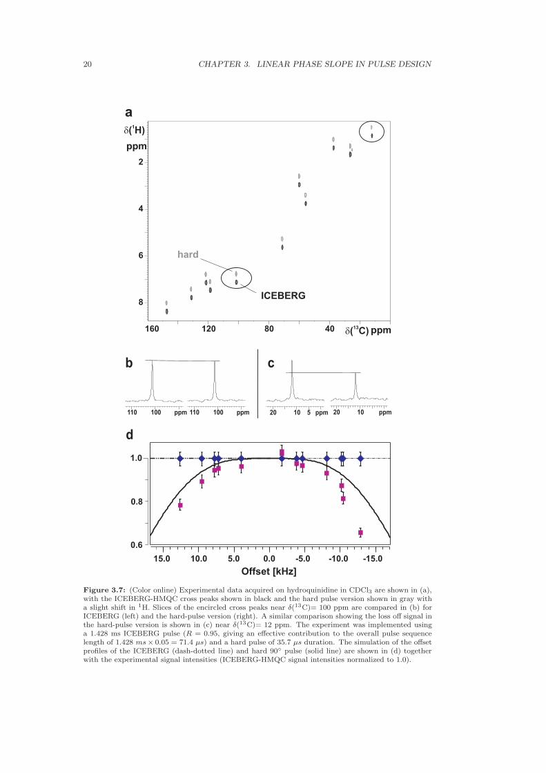
The best broadband refocusing performance available in the standard Bruker pulse lib-rary satisfying the required conservative pulse power limits is obtained using the pulsedesignated Chirp80 [21]. This pulse is constructed from three adiabatic inversion pulseswith pulse lengths in the ratio 1:2:1 [40]. It utilizes for its shortest element a 500 mssmoothed chirp pulse [64] with 80 kHz sweep. The first 20% of the pulse rises smoothlyto a maximum constant RF amplitude of 11.26 kHz according to a sine function beforedecreasing in the same fashion to zero during the final 20% of the pulse. The final pulseis thus 2 ms long (Fig. 4.1).
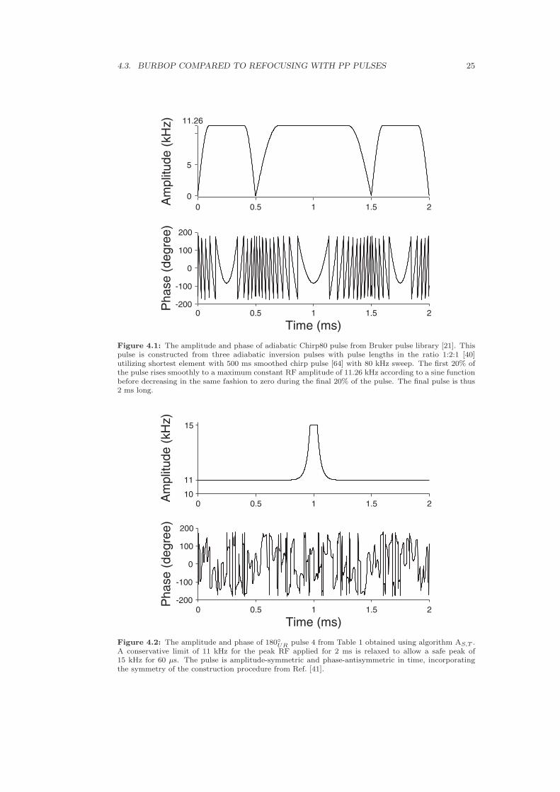
Maintaining this pulse length and mindful of the given conservative peak RF amp-litude, we designed the set of four pulses listed in Table 1. For most of the pulse,the nominal RF amplitude is a constant 10 or 11 kHz. A maximum RF amplitude of15 kHz is applied for 60 µs in the middle of the pulse, as illustrated in Fig. 4.2. Thisshort increase in pulse amplitude provides significant improvement in pulse performancecompared to Chirp80.
The amplitude profile shown in Fig. 4.2 is reminiscent of the hyperbolic secantpulse [27], which maintains a low amplitude for most of the pulse with a peak in themiddle. All four pulses show excellent performance over the listed ranges in offset andRF field inhomogeneity/miscalibration. Performance is comparable to the performanceshown in Fig. 4.3 for higher power, constant amplitude pulses with nominal peak RF of15 kHz. Pulse 4 provides the most relevant comparison, since it has a similar range oftolerance to RF inhomogeneity. As expected from the earlier results for algorithms Aand AS , the best amplitude performance is obtained by algorithm AT and the best phaseperformance by algorithm AS,T . Figure 4.4 compares theoretical performance of pulses1 and 4 from Table 1 to the Chirp80 pulse. The new pulses significantly improve phaseperformance over the targeted range of offsets and RF inhomgeneity/miscalibration.Additional quantitative comparison between pulse 4 and Chirp80 are provided in Figs.4.5 and 4.6, 4.8 and 4.9, and 4.10, which also show the excellent agreement betweensimulations and experimental pulse performance. Improvements in lineshape and phasethat are possible using the new pulses are shown in Fig. 4.7.
4.3. BURBOP COMPARED TO REFOCUSING WITH PP PULSES 25
0 0.5 1 1.5 2
0
5A
mp
litu
de
(kH
z)
0 0.5 1 1.5 2-200
-100
0
100
200
Time (ms)
Ph
ase
(d
eg
ree
)
11.26
Figure 4.1: The amplitude and phase of adiabatic Chirp80 pulse from Bruker pulse library [21]. Thispulse is constructed from three adiabatic inversion pulses with pulse lengths in the ratio 1:2:1 [40]utilizing shortest element with 500 ms smoothed chirp pulse [64] with 80 kHz sweep. The first 20% ofthe pulse rises smoothly to a maximum constant RF amplitude of 11.26 kHz according to a sine functionbefore decreasing in the same fashion to zero during the final 20% of the pulse. The final pulse is thus2 ms long.
0 0.5 1 1.5 210
11
Am
plit
ude (
kH
z)
0 0.5 1 1.5 2-200
-100
0
100
200
Time (ms)
Phase (
degre
e)
15
Figure 4.2: The amplitude and phase of 180◦UR pulse 4 from Table 1 obtained using algorithm AS,T .A conservative limit of 11 kHz for the peak RF applied for 2 ms is relaxed to allow a safe peak of15 kHz for 60 µs. The pulse is amplitude-symmetric and phase-antisymmetric in time, incorporatingthe symmetry of the construction procedure from Ref. [41].

26 CHAPTER 4. BROADBAND 180◦ UNIVERSAL ROTATION PULSES
Mz → − M
z
(Transfer Efficiency)
B1 /
B10
0.7
1
1.3
Mx → − M
x
(Transfer Efficiency)
Mx → − M
x
(Phase deviation)
B1 /
B10
0.7
1
1.3
B1 /
B10
0.7
1
1.3
B1 /
B10
Offset (kHz)−20 0 20
0.7
1
1.3
Offset (kHz)−20 0 20
Offset (kHz)−20 0 20
0.98
0.30
0.997
0.98
0.9830.983
0.98
0.50
3.50
80
0.998
0.98
a)
b)
c)
d)
Figure 4.3: (Color online) Theoretical performance of four 180◦UR
pulses for inversion of magnetizationabout the y-axis, designed using different algorithms. The first two columns show the transfer efficiencyfor the labeled transformations relative to ideal or complete transfer. The last column displays phasedeviation in degrees relative to the labeled target state. The nominal peak RF amplitude for all thepulses is B0
1= 15 kHz, optimized to perform over a resonance offset range of 50 kHz and variation in
RF homogeneity/calibration of ±33%. All pulses are constant amplitude with the exception of pulseb), which deviates from the maximum for less than 10% of the pulse. a) constructed from the 1 ms90◦
PPpulse of Ref. [51] preceded by its time- and phase-reversed waveform [41], pulse length Tp = 2 ms.
b) algorithm A, Tp = 2 ms. c) algorithm A, Tp = 1 ms. d) algorithm AS , which incorporates thesymmetry principle used in a), Tp = 2 ms. B1 is the variable RF amplitude.

4.4. EXPERIMENT 27
Pulse Algorithm RFnominal RFmax Inhomogeneity Transformation Error(kHz) (kHz) optimization (amplitude) (phase)
1 AT 11 15 ±10% < 0.2% < 2◦
2 AS,T 11 15 ±15% < 0.9% < 0.3◦
3 AS,T 10 15 ±15% < 1.5% < 0.5◦
4 AS,T 11 15 ±25% < 2% < 0.8◦
Table 4.1: Four pulses optimized to execute a 180◦ universal rotation about the y-axis over resonanceoffsets of 50 kHz and RF field inhomogeneity listed in column 5. All pulses are 2 ms long. For all but60 µs, pulse RF is constant at the value RFnominal, increasing to RFmax in the middle of the pulse(see Fig. 4.2). Amplitude errors in the transformation are the maximum deviation from the targetmagnetization over the optimized ranges of resonance offset and RF inhomogeneity, expressed as apercent. Similarly, phase errors represent the maximum deviation from the target phase. Performanceof pulses 1 and 4 are shown in more detail in Fig. 4.4.
4.4 Experiment
All experiments were implemented on a Bruker 750 MHz Avance III spectrometerequipped with SGU units for RF control and linearized amplifiers, utilizing a triple-resonance PATXI probehead and gradients along the z-axis. Measurements are theresidual HDO signal in a sample of 99.96% D2O doped with CuSO4 to a T1 relaxa-tion time of 100 ms at 298◦ K. Signals were obtained at offsets between −25 kHz to25 kHz in steps of 500 Hz. To demonstrate the tolerance of the pulses to RF inhomo-geneity/miscalibration, the experiments were repeated with RF amplitude incrementedby ±15% and ±25% relative to the nominal maximum RF amplitude for each pulse(15 kHz for pulse 4 of Table 1, 11.26 kHz for Chirp80). To reduce the effects of RFfield inhomogeneity within the coil itself, approximately 40 µl of the sample solutionwas placed in a 5 mm Shigemi limited volume tube.
4.5 Conclusion
We have presented three optimal control algorithms for the de novo design of universalrotation pulses, applied specifically to inversion. The most noteworthy innovations forNMR spectroscopy are inclusion of the construction principle discovered in [41] and atime-dependent or “floating” limit on the peak RF allowed during the pulse. The newalgorithms result in improved performance compared to existing UR pulses constructedas composites of point-to-point pulses. The methodology is very general, and furtherimprovements in the design of robust universal rotation pulses can be anticipated. Thenew pulses are implemented in the Bruker pulse library and will also be made availablefor downloading from the website
http://www.org.chemie.tu-muenchen.de/glaser/Downloads.html.

28 CHAPTER 4. BROADBAND 180◦ UNIVERSAL ROTATION PULSES
Figure 4.4: (Color online) Similar to Fig. 4.3, but the maximum RF amplitude is allowed to float for asufficiently short time period, giving the reduced-power pulse in Fig. 4.2. All three pulses are designedto operate over a resonance offset of 50 kHz and a range of variation in RF homogeneity/calibrationrelative to the ideal B0
1, as given in Table 1. a) pulse 1 of Table 1, RF tolerance ±10%. b) pulse 4
of Table 1, RF tolerance ±25%. c) composite adiabatic refocusing [40] using pulse Chirp80 from theBruker pulse library [21].
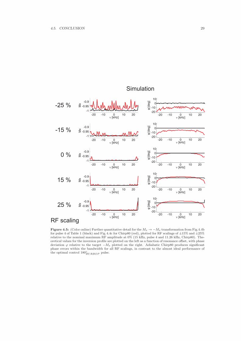
4.5. CONCLUSION 29
RF scaling
-25 %
-15 %
0 %
15 %
25 %
-20 -10 0 10 20
-1
-0.95
-0.9
n [kHz]
Mx
-20 -10 0 10 20-20
-10
0
10
n [kHz]
φ[d
eg]
-20 -10 0 10 20
-1
-0.95
-0.9
n [kHz]
Mx
-20 -10 0 10 20-20
-10
0
10
n [kHz]
φ[d
eg]
-20 -10 0 10 20
-1
-0.95
-0.9
n [kHz]
Mx
-20 -10 0 10 20-20
-10
0
10
n [kHz]
φ[d
eg]
-20 -10 0 10 20
-1
-0.95
-0.9
n [kHz]
Mx
-20 -10 0 10 20-20
-10
0
10
n [kHz]
φ[d
eg]
-20 -10 0 10 20
-1
-0.95
-0.9
n [kHz]
Mx
-20 -10 0 10 20-20
-10
0
10
n [kHz]
φ[d
eg]
Simulation
Figure 4.5: (Color online) Further quantitative detail for the Mx → −Mx transformation from Fig.4.4bfor pulse 4 of Table 1 (black) and Fig.4.4c for Chirp80 (red), plotted for RF scalings of ±15% and ±25%relative to the nominal maximum RF amplitude at 0% (15 kHz, pulse 4 and 11.26 kHz, Chirp80). The-oretical values for the inversion profile are plotted on the left as a function of resonance offset, with phasedeviation ϕ relative to the target −Mx plotted on the right. Adiabatic Chirp80 produces significantphase errors within the bandwidth for all RF scalings, in contrast to the almost ideal performance ofthe optimal control 180◦
BURBOPpulse.

30 CHAPTER 4. BROADBAND 180◦ UNIVERSAL ROTATION PULSES
RF scaling
-25 %
-15 %
0 %
15 %
25 %
-20 -10 0 10 20
-1
-0.95
-0.9
n [kHz]
Mx
-20 -10 0 10 20-20
-10
0
10
n [kHz]
φ[d
eg]
-20 -10 0 10 20
-1
-0.95
-0.9
n [kHz]
Mx
-20 -10 0 10 20-20
-10
0
10
n [kHz]
φ[d
eg]
-20 -10 0 10 20
-1
-0.95
-0.9
n [kHz]
Mx
-20 -10 0 10 20-20
-10
0
10
n [kHz]
φ[d
eg]
-20 -10 0 10 20
-1
-0.95
-0.9
n [kHz]
Mx
-20 -10 0 10 20-20
-10
0
10
n [kHz]
φ[d
eg]
-20 -10 0 10 20
-1
-0.95
-0.9
n [kHz]
Mx
-20 -10 0 10 20-20
-10
0
10
n [kHz]
φ[d
eg]
Experiment
Figure 4.6: (Color online) Experimental measurements of the inversion profile (left) and phase de-viation (right) corresponding to the simulations in Fig. 4.5, showing excellent agreement between theexperimental and theoretical performance of the pulses.

4.5.
CONCLUSIO
N31
Adiabatic
Optimal control
-25 % -15 % 0 % 15 % 25 %RF scalingFigure 4.7: Experimental lineshapes (black) comparing optimal control 180◦
URpulse 4 of Table 1 and adiabatic Chirp80 at a resonance offset of −25 kHz for RF
scalings of ±15% and ±25% relative to the nominal maximum RF amplitude of 15 kHz at 0%. Simulations (gray) are in excellent agreement with the experiments,as already shown in Figures 4.5 and 4.6. Chirp80 produces significant experimental phase errors of 20◦, 15◦, 9◦, 11◦, and 5◦(reading left-to-right across the RFscalings in the figure) in contrast to the experimental performance of 0.7◦, 0.7◦, 0.9◦, 2.6◦, 2.5◦ for the optimal control 180◦BURBOP pulse.

32 CHAPTER 4. BROADBAND 180◦ UNIVERSAL ROTATION PULSES
RF scaling
-25 %
-15 %
0 %
15 %
25 %
φφ
φφ
φ
Simulation
Figure 4.8: (Color online) Further quantitative detail for the My → My transformation for pulse 4 ofTable 1 (black) and Fig.4.4c for Chirp80 (red), plotted for RF scalings of ±15% and ±25% relative to thenominal maximum RF amplitude at 0% (15 kHz, pulse 4 and 11.26 kHz, Chirp80). Theoretical valuesfor the inversion profile are plotted on the left as a function of resonance offset, with phase deviationϕ relative to the target My plotted on the right. Adiabatic Chirp80 produces significant phase errorswithin the bandwidth for all RF scalings, in contrast to the almost ideal performance of the optimalcontrol.

4.5. CONCLUSION 33
RF scaling
-25 %
-15 %
0 %
15 %
25 %
φφ
φφ
φ
Experiment
Figure 4.9: (Color online) Experimental measurements of the inversion profile (left) and phase de-viation (right) corresponding to the simulations in Fig. 4.8, showing excellent agreement between theexperimental and theoretical performance of the pulses.

34 CHAPTER 4. BROADBAND 180◦ UNIVERSAL ROTATION PULSES
RF scaling
-25 %
-15 %
0 %
15 %
25 %
Simulation Experiment
Figure 4.10: (Color online) Further quantitative detail for the Mz → −Mz transformation fromFig. 4.4b for pulse 4 of Table 1 (black) and Fig. 4.4c for Chirp80 (red), plotted for RF scalings of ±15%and ±25% relative to the nominal maximum RF amplitude at 0% (15 kHz, pulse 4 and 11.26 kHz,Chirp80). Theoretical and experimental values for the inversion profile are plotted as a function ofresonance offset. Experimental measurements of the inversion profile corresponding to the simulations,showing excellent agreement between the experimental and theoretical performance of the pulses.

Chapter 5
Band-selective excitationpulsesthat accommodate relaxationand RF inhomogeneity
5.1 Introduction
This chapter is a part of an article [65] submitted to Journal of Magnetic Resonance.Frequency-selective pulses have widespread utility in magnetic resonance and have mo-tivated significant efforts towards their design [66–111]. In many useful cases, the res-ulting methodologies can achieve the best approximation to the ideal rectangular profilefor spin response as a function of frequency offset.
However, in all of these approaches to pulse design, performance criteria that can beincluded in the design protocol are restricted either by analytical procedures of highlyspecific scope or by numerical methods that are limited by the efficiency of the optimiz-ations employed. As a result, pulse response is typically optimized only for the nominalideal RF pulse values. In addition, although the length of pulses required for narrow-band applications can significantly reduce their effectiveness when relaxation times arecomparable to the pulse length [112, 113], the solution to the problem—selective pulseswhich are less sensitive to relaxation effects—can also be demanding for standard designmethods [97, 114–118].
To make these design challenges tractable, the space of possible pulse shapes is oftenreduced by forcing the solution to be a member of a particular family of functional forms(for example, finite Fourier series). Thus, potentially, there are important solutions thatare missed. Over the past decade, we have shown optimal control theory to be an efficientand powerful method that can be applied to a wide range of challenging NMR pulsedesign problems without restricting the space of possible solutions [48–53,56,57,119–129].It is capable of designing broadband pulses [52] and selective pulses [130, 131] that aresimultaneously tolerant to RF inhomogeneity and relaxation effects, which we developfurther in the present chapter.
35

36CHAPTER 5. BAND-SELECTIVE EXCITATION PULSES
THAT ACCOMMODATE RELAXATION AND RF INHOMOGENEITY
5.2 Selective pulse design
Optimal control (including similar, related optimization procedures) was originally in-troduced into magnetic resonance for the design of band-selective pulses, primarily forimaging [43,44,47,132–135]. It was quickly supplanted by the efficient Shinnar-LeRoux(SLR) algorithm [82–85, 136], which establishes a correspondence between frequency-selective pulse design and digital filter design. There are fast, non-iterative algorithmsfor the ideal filter and, hence, the ideal pulse. Unfortunately, the algorithm does notaccommodate additional criteria, such as tolerance to RF inhomogeneity (included insome of the earliest optimal control-related approaches [132, 134]) or relaxation effects.In addition, the most applicable and widely used form of the algorithm derives pulseswhich produce a specific linear phase dispersion in the spectral response. Pulses produ-cing no phase dispersion, suitable for spectroscopy, are more problematic for the SLRalgorithm.
We first provide an overview of well-known issues relevant to selective pulse design,since there is considerably less freedom in the choice of parameters compared to broad-band pulses. For example, in designing broadband pulses, we have shown [122] there isat best only a marginal relation between the maximum amplitude, RFmax, of a pulseand the achievable excitation or inversion bandwidth, as long as the pulse length, Tp,is allowed to increase sufficiently. Alternatively, increasing RFmax for a given Tp canimprove performance for a given bandwidth or increase the bandwidth. There can alsobe innumerable broadband pulses that provide approximately equal performance for agiven RFmax, Tp, and bandwidth.
Selective pulses are far more constrained, with a well-known relation between theselective bandwidth and Tp, and much tighter limits on the choice of RFmax for agiven product of bandwidth and Tp [136]. We provide only a simple overview of theoptimal control methodology, emphasizing the modifications necessary for the presentchapter. The basic algorithm for optimizing pulse performance over a range of resonanceoffsets and RF inhomogeneity is described fully in [48]. Details related to incorporatingrelaxation [52] and specific dispersion in the phase of the final magnetization [45,50,53],which we refer to as the phase slope, are provided in the associated references.
5.2.1 Phase slope
Following the Chapter 3, values of the phase slope, R, [53] at each offset characterizethe net phase dispersion that accumulates during a pulse of length Tp. The phaseslope is defined relative to the net precession of transverse magnetization that would beproduced solely by chemical-shift evolution during the same time interval, Tp. A pulsethat produces focused magnetization of fixed phase for all spins in the offset range ofinterest would have constant R = 0 (i.e., a self-refocused pulse). Many selective pulsesare symmetric, R = 1/2 pulses [43,72,91,93,94,136]. The symmetry of the resulting pulseprovides an advantage in the development of various algorithms used in selective pulsedesign, such as SLR, inverse scattering [86, 91], polychromatic [93], and stereographicprojection [94]. In fact, the standard form of the SLR algorithm [136] can only generatelinear phase of this value. Sophisticated algorithms allowing for more general phasein selective pulses are described in the literature [90, 137, 138], but they are specific tothis particular performance factor and cannot include tolerance to variations in otherexperimentally important parameters.
By contrast, including additional performance criteria, such as a general phase re-sponse, is straightforward for optimal control. Initial magnetization M (t0) is driven by

5.2. SELECTIVE PULSE DESIGN 37
the RF controls to a final magnetization ~F that is defined for each resonance offset in thedesired range. To excite transverse magnetization of linear phase slope R, we considertarget states for each offset ∆ν in the excitation bandwidth of the form [53]
~F = [ cos(ϕ), sin(ϕ), 0 ] (5.1)
Choosing ϕ = R∆νTp gives a linear phase slope, but any function can be considered todefine a useful target phase, such as quadratic or higher order.
Selective excitation most simply requires changing the target to ~F = [ 0, 0, 1 ] for off-sets outside the desired bandwidth. However, since the ideal rectangular offset responsecan not be excited by a finite-length pulse, there must be a transition connecting theexcitation frequencies to the nulled frequencies. This is typically defined in terms ofdesign parameters for finite impulse response (FIR) filters. An overview of the issuesrelevant to our optimal control implementation follows.
5.2.2 Selective pulses as digital filters
For design conditions employing ideal RF in the absence of relaxation, selective pulseperformance is completely determined by the desired passband width B, pulse length Tp,transition width W joining the passband and stopband, and residual signal fluctuationor ripple δ1 and δ2 about the ideal target amplitude for the passband and stopband,respectively.
The passband frequency νp and stopband frequency νs are defined where the mag-nitude of the magnetization response becomes less than the associated fluctuations 1−δ1and |δ2|, as illustrated in Fig. 5.1 (adopted from Ref. [136]). The frequency where theamplitude drops to one-half is approximately the average of these two frequencies. Thefull width of the filter is defined as twice this value, giving a bandwidth B = νs+ νp anda fractional transition width W = (νs − νp)/B.
More specifically (and again emphasizing the design conditions stated at the begin-ning of the section), selective pulse performance is constrained by relations for optimalFIR filters of the form [139]
WTpB = f(δ1, δ2), (5.2)
in terms of an empirically derived function f(δ1, δ2). For a given value of f = WTpB,smaller (larger) δ1 gives larger (smaller) δ2. Alternatively, for fixed δ1 or fixed δ2, valuesof f increase as δ2 or δ1, respectively, decrease. Flexibility in selective pulse designis thus purchased at the cost of trade-offs among bandwidth, pulse length, transitionwidth, and ripple amplitudes. Choosing any four of the set determines the fifth.
This relation appears to have been little used in the spectroscopic community. Al-though the precise form of the function f(δ1, δ2) holds only for R = 1/2 pulses, we havefound it to be a useful qualitative indicator for more general R. One important implica-tion is that pulse performance for a given absolute transition width BW = νs−νp can bemade independent of the passband width, B. Fixed Tp results in the same performancein terms of residual signal (ripple) for different B as long as BW is constant. This wasobserved empirically and noted in [111]. We thus use Eq. 5.2 to inform our optimalcontrol design.
5.2.3 Optimal control
The approximation to the ideal rectangular frequency response profile, as illustrated inFig. 5.1, can be readily obtained using a variety of methods—among them, the Parks-McClellan (PM) algorithm for linear-phase FIR digital filters [139]. After calculating the

38CHAPTER 5. BAND-SELECTIVE EXCITATION PULSES
THAT ACCOMMODATE RELAXATION AND RF INHOMOGENEITY
±δ2
νp
νs
1
0
δ1
Figure 5.1: (Color online, Adapted from Ref. [136]) A finite length selective pulse can only approximatethe ideal rectangular frequency response. Residual signal or ripple amplitude in the selected frequencyspectrum (passband) is denoted by δ1, with δ2 representing the ripple over the frequency range wherethe signal should be nulled (stopband). The positive frequencies νp and νs define the passband andstopband, respectively. The plotted response is symmetric about the zero frequency.
PM polynomial, the standard SLR algorithm effectively inverts the frequency responseto produce a linear phase (R = 1/2) RF pulse. The equivalent optimal control approachwould be to use the polynomial response function as the target response and efficientlymodify the RF controls to achieve the allowed performance.
However, as noted already, the target response derived using the PM algorithmapplies only to R = 1/2, using the ideal RF amplitudes, in the absence of relaxation.More significantly, optimal control does not need to know the polynomial response. Onecan simply define the ideal passband/stopband frequency response, and the algorithmwill find the response allowed by the particular choice of bandwidth, pulse length, andtransition width. Different functional forms can be defined for the response in thetransition region to provide additional flexibility. The response at each frequency canalso be given weights to fine-tune the final excitation profile.
We now proceed with the design of more robust selective excitation pulses. In whatfollows, we let the frequency response to the pulse (ie, the target function) be undefinedin the transition region. The pulse has the flexibility to do anything it wants there. Animportant addition to the algorithm is an adjustable weight function, which changes theweight for each particular offset depending on the deviation of intermediate results fromthe desired performance. During a given iteration, if the deviation of magnetizationfrom the target for a particular offset is larger than the allowed ripple amplitude, thenthe weight for this offset increases; otherwise it decreases.
5.3 Results and Discussion
We present several examples illustrating the advantages of selective excitation by op-timized pulses (SEBOP). As discussed, possible performance improvements include in-creased tolerance to RF inhomogeneity and compensation for relaxation effects.

5.3. RESULTS AND DISCUSSION 39
5.3.1 Tolerance to RF inhomogeneity
As a first example, consider a representative imaging pulse from Ref. [136], designedusing the SLR algorithm to selectively excite a bandwidth B = 2 kHz with a transitionwidth W = 0.18, pulse length Tp = 4 ms, and stopband ripple δ2 = 1%, resulting ina passband ripple δ1 = 1% from the relation referenced in Eq. 5.2. The amplitude-modulated pulse and its theoretical spectral response are shown in Fig. 5.2. RF inhomo-geneity in the range ±20% results in signal variations in the passband of ∼10–15%.
Tolerance to RF inhomogeneity is considerably more difficult to achieve for selectivecompared to broadband pulses, due to the much tighter constraints required for selectiv-ity. Nonetheless, allowing ±20% pulse miscalibration in the optimal control algorithmresults in the two-component amplitude- and phase-modulated SEBOP pulse shown onthe right in Fig. 5.2. For an average power equal to 95% of the SLR pulse average powerand the same phase slope R = 1/2, SEBOP reduces passband signal variation due to thespecified RF inhomogeneity to less than ∼5%. Stopband ripple, which corrupts imagefidelity due to signal outside the selected frequencies (out-of-slice signal), is also reducedconsiderably.
In contrast to imaging, selective pulses for high resolution NMR are of greatest utilityif they are refocused pulses, which produce no phase gradient in the spectrum (phaseslope R = 0 in our terminology). This will be the case for all the examples which follow.
5.3.2 Compensation for relaxation and RF inhomogeneity
The algorithm for generating relaxation compensated broadband pulses (RC-BEBOP)has already been developed [52]. It only needs inclusion of the modified target functionsdescribed in Section 5.2.1 for application to selective pulses (RC-SEBOP). The primaryresult of that work is that substantial signal gains are possible relative to expectedlosses from short T1, T2 by finding trajectories for the transformed magnetization thatminimize these losses, even if this requires a longer pulse length. Relaxation losses areminimized by keeping spins near the z-axis and orienting them so that all offsets can betransformed to the transverse plane in a very short time at the end of the pulse. Thissolution not only mitigates the effects of transverse relaxation, but short T1 becomesan advantage due to repolarization of z-magnetization during the relatively long timethe spins are aligned close to the longitudinal axis. The net affect is that almost allthe RF power is applied at the end of our relaxation compensated pulses [52]. This isfortunately also consistent with a particular family of solutions for broadband R = 0(refocused) pulses [53].
There are also solutions for refocused selective excitation pulses [111] that employsignificant RF power throughout the pulse and therefore do not lend themselves to relax-ation compensation. On the other hand, these pulses do an excellent job of minimizingthe residual off-axis magnetization in both the passband and stopband. Consistent withthis result, we find empirically that minimizing relaxation losses for selective pulsescompetes with minimizing residual off-axis magnetization. The trajectories that reducerelaxation effects are not compatible with those that achieve good refocusing. We there-fore consider a strategy that maximizes x-magnetization in the passband, minimizesit in the stopband, i.e., the standard procedure, but removes any explicit restrictionson residual y-magnetization. This allows the optimal control algorithm to emphasizerelaxation compensation and find solutions with considerably enhanced performancecompared to those that give highest priority to minimizing the y-component. As we willshow, this undesirable residual magnetization can be eliminated after the pulse withoutsignificantly affecting performance.

40CHAPTER 5. BAND-SELECTIVE EXCITATION PULSES
THAT ACCOMMODATE RELAXATION AND RF INHOMOGENEITY
0 1 2 3 4−0.2
0
0.2
0.4
0.6
RF
Am
plitu
de (
kHz)
Time (ms)0 1 2 3 4
−0.4
−0.2
0
0.2
0.4
0.6
−5 0 50
0.5
1
Tra
nsve
rse
Mag
netiz
atio
n −5 0 50
0.5
1
−5 −4 −3 −2 −1
0
0.05
0.1
−5 −4 −3 −2 −1
0
0.05
0.1
−1 −0.5 0 0.5 10.8
0.85
0.9
0.95
1
−1 −0.5 0 0.5 10.8
0.85
0.9
0.95
1
Frequency (kHz)
Figure 5.2: (Color online) Panels on the left show an amplitude modulated selective pulse producedby the SLR algorithm, which can not explicitly incorporate tolerance to RF inhomogeneity, followedbelow by its theoretical frequency response, a magnified view of the stopband, and a magnified view ofthe passband. Values of the simulated RF miscalibration/inhomogeneity are −20% (blue), 0% (green),and +20% (red). Similarly, panels on the right show the x-phase (blue) and y-phase (green) RFcomponents of an amplitude- and phase-modulated SEBOP pulse, followed by its frequency response.Design parameters and average power (see Section 5.3.1) are the same for both pulses.
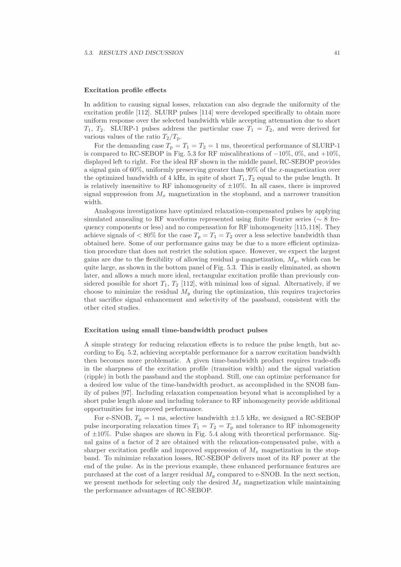
5.3. RESULTS AND DISCUSSION 41
Excitation profile effects
In addition to causing signal losses, relaxation can also degrade the uniformity of theexcitation profile [112]. SLURP pulses [114] were developed specifically to obtain moreuniform response over the selected bandwidth while accepting attenuation due to shortT1, T2. SLURP-1 pulses address the particular case T1 = T2, and were derived forvarious values of the ratio T2/Tp.
For the demanding case Tp = T1 = T2 = 1 ms, theoretical performance of SLURP-1is compared to RC-SEBOP in Fig. 5.3 for RF miscalibrations of −10%, 0%, and +10%,displayed left to right. For the ideal RF shown in the middle panel, RC-SEBOP providesa signal gain of 60%, uniformly preserving greater than 90% of the x-magnetization overthe optimized bandwidth of 4 kHz, in spite of short T1, T2 equal to the pulse length. Itis relatively insensitive to RF inhomogeneity of ±10%. In all cases, there is improvedsignal suppression from Mx magnetization in the stopband, and a narrower transitionwidth.
Analogous investigations have optimized relaxation-compensated pulses by applyingsimulated annealing to RF waveforms represented using finite Fourier series (∼ 8 fre-quency components or less) and no compensation for RF inhomogeneity [115,118]. Theyachieve signals of < 80% for the case Tp = T1 = T2 over a less selective bandwidth thanobtained here. Some of our performance gains may be due to a more efficient optimiza-tion procedure that does not restrict the solution space. However, we expect the largestgains are due to the flexibility of allowing residual y-magnetization, My, which can bequite large, as shown in the bottom panel of Fig. 5.3. This is easily eliminated, as shownlater, and allows a much more ideal, rectangular excitation profile than previously con-sidered possible for short T1, T2 [112], with minimal loss of signal. Alternatively, if wechoose to minimize the residual My during the optimization, this requires trajectoriesthat sacrifice signal enhancement and selectivity of the passband, consistent with theother cited studies.
Excitation using small time-bandwidth product pulses
A simple strategy for reducing relaxation effects is to reduce the pulse length, but ac-cording to Eq. 5.2, achieving acceptable performance for a narrow excitation bandwidththen becomes more problematic. A given time-bandwidth product requires trade-offsin the sharpness of the excitation profile (transition width) and the signal variation(ripple) in both the passband and the stopband. Still, one can optimize performance fora desired low value of the time-bandwidth product, as accomplished in the SNOB fam-ily of pulses [97]. Including relaxation compensation beyond what is accomplished by ashort pulse length alone and including tolerance to RF inhomogeneity provide additionalopportunities for improved performance.
For e-SNOB, Tp = 1 ms, selective bandwidth ±1.5 kHz, we designed a RC-SEBOPpulse incorporating relaxation times T1 = T2 = Tp and tolerance to RF inhomogeneityof ±10%. Pulse shapes are shown in Fig. 5.4 along with theoretical performance. Sig-nal gains of a factor of 2 are obtained with the relaxation-compensated pulse, with asharper excitation profile and improved suppression of Mx magnetization in the stop-band. To minimize relaxation losses, RC-SEBOP delivers most of its RF power at theend of the pulse. As in the previous example, these enhanced performance features arepurchased at the cost of a larger residual My compared to e-SNOB. In the next section,we present methods for selecting only the desired Mx magnetization while maintainingthe performance advantages of RC-SEBOP.

42
CHAPTER
5.
BAND-SELECTIV
EEXCIT
ATIO
NPULSES
THAT
ACCOMMODATE
RELAXATIO
NAND
RF
INHOMOGENEIT
Y
−15 −10 −5 0 5 10 15
0
0.2
0.4
0.6
0.8
1
Mx
−15 −10 −5 0 5 10 15
0
0.2
0.4
0.6
0.8
1
−15 −10 −5 0 5 10 15
0
0.2
0.4
0.6
0.8
1
−15 −10 −5 0 5 10 15−1
−0.5
0
0.5
1
My
−15 −10 −5 0 5 10 15−1
−0.5
0
0.5
1
Frequency (kHz)−15 −10 −5 0 5 10 15
−1
−0.5
0
0.5
1
B1/B
10=0.9 B
1/B
10=1 B
1/B
10=1.1
Figure 5.3: (Color online) Excited magnetization Mx (top panels) and My (bottom panels) is plotted as a function of resonance offset for SLURP-1 (green)and RC-SEBOP (blue) for Tp = T1 = T2 = 1 ms and RF inhomogeneity/miscalibration of −10%, 0%, +10% reading left to right. Despite these fast relaxationrates, RC-SEBOP preserves >90% of the desired Mx while achieving a nearly rectangular profile that is relatively insensitive to ±10% RF inhomogeneity over theoptimized excitation bandwidth of 3 kHz. The signal gain on resonance for the nominal ideal RF is a factor of 1.6. Minimal relaxation losses are achieved byallowing large residual My, particularly in the stopband. This unwanted signal can be subsequently eliminated without affecting performance, as described in thetext (see Fig. 5.5).
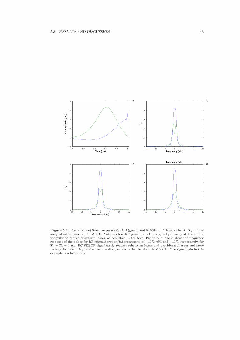
5.3. RESULTS AND DISCUSSION 43
0 0.2 0.4 0.6 0.8 1−0.5
0
0.5
1
1.5
2
RF
Am
plitu
de (
kHz)
Time (ms)−15 −10 −5 0 5 10 150
0.2
0.4
0.6
0.8
1
Mx
Frequency (kHz)
−15 −10 −5 0 5 10 150
0.2
0.4
0.6
0.8
1
Mx
Frequency (kHz)−15 −10 −5 0 5 10 150
0.2
0.4
0.6
0.8
1Frequency (kHz)
d
b
c
a
Figure 5.4: (Color online) Selective pulses eSNOB (green) and RC-SEBOP (blue) of length Tp = 1 msare plotted in panel a. RC-SEBOP utilizes less RF power, which is applied primarily at the end ofthe pulse to reduce relaxation losses, as described in the text. Panels b, c, and d show the frequencyresponse of the pulses for RF miscalibaration/inhomogeneity of −10%, 0%, and +10%, respectively, forT1 = T2 = 1 ms. RC-SEBOP significantly reduces relaxation losses and provides a sharper and morerectangular selectivity profile over the designed excitation bandwidth of 3 kHz. The signal gain in thisexample is a factor of 2.

44CHAPTER 5. BAND-SELECTIVE EXCITATION PULSES
THAT ACCOMMODATE RELAXATION AND RF INHOMOGENEITY
5.4 Experimental
All the selective pulses considered so far produce significant residual My magnetizationin the passband at non-ideal RF calibration. Methods for removing this unwanted signaltherefore have more general applicability.
To destroy undesired My after selective excitation in a single-acquistion experiment,a hard 90◦−y flip-back pulse can be applied to store Mx along the z-axis. A gradientpulse is then employed to dephase the My component, followed by a hard 90◦y pulse foracquisition of the signal due to Mx. This “crusher” sequence, implemented in Fig. 5.5aas a more general phase-cycled sequence (to be discussed below), was first tested forthe case of unlimited-bandwidth hard pulses by applying the hard pulses on resonance.The transmitter frequency was shifted only for the RC-SEBOP pulse to measure it’soff-resonance performance. This sequence is insensitive to the actual T2 of the sample,since there is minimal relaxation during the short hard pulses and no T2 relaxation ofmagnetization stored along the z-axis during the gradient pulse. In addition, for typicalsamples with T1 ≫ T2, there are minimal T1 effects as a result of the sequence. However,for very short T1, repolarization of stopband magnetization during the gradient pulsecan lead to slightly more Mx magnetization in the stopband than expected from thetheoretical selectivity profile of RC-BEBOP, previously illustrated in Fig. 5.4.
To eliminate extra stopband signal in cases where T1 is too short for ideal performanceof the original crusher sequence, it can be phase-cycled as shown in the figure. The twoacquisitions add constructively in the passband. Repolarization at stopband frequenciesleads to +z-magnetization after the first hard pulse in each cycle which is canceled byaddition of the two acquisitions after the second hard pulse. As a general strategy, thissequence works very well for the case of ideal hard pulses with no bandwidth limitations.It therefore also works well over a bandwidth of ∼ 8 kHz for a 25 kHz hard pulse, wherethe performance of the hard pulse is sufficiently ideal, and may be useful for applicationsthat require only a relatively narrow range of stopband frequencies compared to theavailable RF amplitude of the hard pulse.
More realistically, all pulses have to be applied at the same transmitter frequency tomeasure the performance of the sequence at larger resonance offsets. The effective fieldof the hard pulses will then have a significant z-component, and the y-magnetizationwill no longer remain untouched. However, the gradient still dephases the transversemagnetization remaining after the first hard pulse. To a first approximation, thereis only z-magnetization prior to the second hard pulse, and the phase cycle producestransverse components of opposite sign that cancel on addition.
Experimental off-resonance performance of RC-SEBOP and the phase-cycled crushersequence is demonstrated in Fig. 5.6 for the residual HDO signal in a sample of 99.96%D2O, doped with CuSO4 to relaxation times of T1 = 1.345 ms and T2 = 1.024 ms at298◦ K. Signals were obtained at offsets between −15 kHz to 15 kHz in steps of 200 Hz.The sequence was first implemented using 10 µs hard pulses, which resulted in stopbandsignal of 5% relative to the centerband. It was then fine-tuned by increasing the hard-pulse length to 10.68 µs in the first cycle. The resulting selectivity profile is in very goodagreement with the simulations for eSNOB and RC-BEBOP performance in Fig. 5.4. Weobtain a signal of 0.83 on resonance using the nominal ideal RF values for RC-SEBOPcompared to the theoretical value 0.89. All values are relative to an ideal signal of 1 forthe case of no relaxation. The small disagreement between experiment and simulationcan be attributed to RF inhomogeneity/miscalibration in the flip-back pulse, which willleave some small fraction of the desired passband signal in the transverse plane to bedestroyed by the gradient.
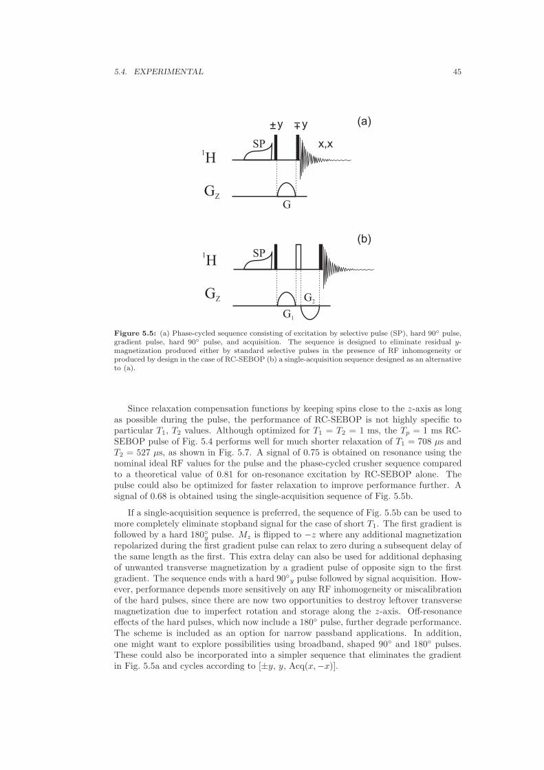
5.4. EXPERIMENTAL 45
1H
G1
G2GZ
SP
1H
GGZ
SP
±
±yy (a)
(b)
x,x
Figure 5.5: (a) Phase-cycled sequence consisting of excitation by selective pulse (SP), hard 90◦ pulse,gradient pulse, hard 90◦ pulse, and acquisition. The sequence is designed to eliminate residual y-magnetization produced either by standard selective pulses in the presence of RF inhomogeneity orproduced by design in the case of RC-SEBOP (b) a single-acquisition sequence designed as an alternativeto (a).
Since relaxation compensation functions by keeping spins close to the z-axis as longas possible during the pulse, the performance of RC-SEBOP is not highly specific toparticular T1, T2 values. Although optimized for T1 = T2 = 1 ms, the Tp = 1 ms RC-SEBOP pulse of Fig. 5.4 performs well for much shorter relaxation of T1 = 708 µs andT2 = 527 µs, as shown in Fig. 5.7. A signal of 0.75 is obtained on resonance using thenominal ideal RF values for the pulse and the phase-cycled crusher sequence comparedto a theoretical value of 0.81 for on-resonance excitation by RC-SEBOP alone. Thepulse could also be optimized for faster relaxation to improve performance further. Asignal of 0.68 is obtained using the single-acquisition sequence of Fig. 5.5b.
If a single-acquisition sequence is preferred, the sequence of Fig. 5.5b can be used tomore completely eliminate stopband signal for the case of short T1. The first gradient isfollowed by a hard 180◦y pulse. Mz is flipped to −z where any additional magnetizationrepolarized during the first gradient pulse can relax to zero during a subsequent delay ofthe same length as the first. This extra delay can also be used for additional dephasingof unwanted transverse magnetization by a gradient pulse of opposite sign to the firstgradient. The sequence ends with a hard 90◦y pulse followed by signal acquisition. How-ever, performance depends more sensitively on any RF inhomogeneity or miscalibrationof the hard pulses, since there are now two opportunities to destroy leftover transversemagnetization due to imperfect rotation and storage along the z-axis. Off-resonanceeffects of the hard pulses, which now include a 180◦ pulse, further degrade performance.The scheme is included as an option for narrow passband applications. In addition,one might want to explore possibilities using broadband, shaped 90◦ and 180◦ pulses.These could also be incorporated into a simpler sequence that eliminates the gradientin Fig. 5.5a and cycles according to [±y, y, Acq(x,−x)].
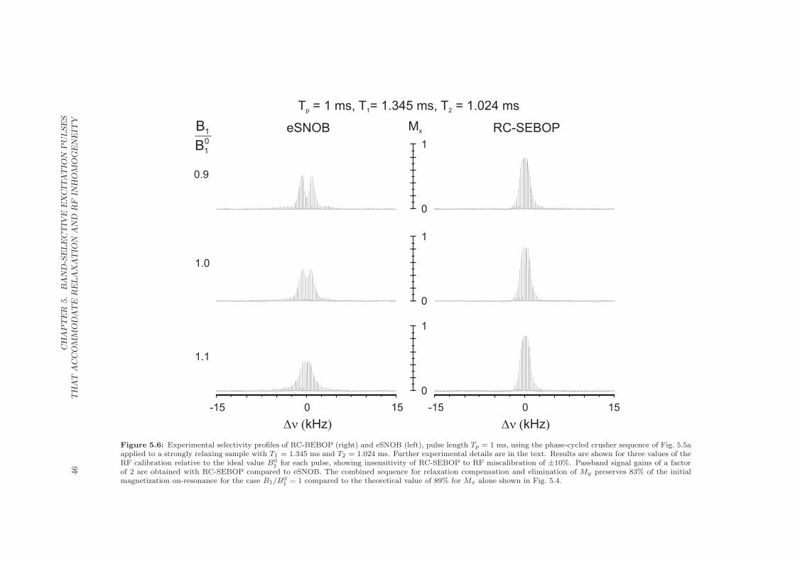
46
CHAPTER
5.
BAND-SELECTIV
EEXCIT
ATIO
NPULSES
THAT
ACCOMMODATE
RELAXATIO
NAND
RF
INHOMOGENEIT
Y
0.9
1.0
1.1
-15 0 15 -15 0 15
Dn ( )kHz Dn ( )kHz
0
1
0
1
0
1
Mx
0
1
1
B
B eSNOB RC-SEBOP
T = 1 ms, T = 1.345 ms, T = 1.024 msp 1 2
Figure 5.6: Experimental selectivity profiles of RC-BEBOP (right) and eSNOB (left), pulse length Tp = 1 ms, using the phase-cycled crusher sequence of Fig. 5.5aapplied to a strongly relaxing sample with T1 = 1.345 ms and T2 = 1.024 ms. Further experimental details are in the text. Results are shown for three values of theRF calibration relative to the ideal value B0
1for each pulse, showing insensitivity of RC-SEBOP to RF miscalibration of ±10%. Passband signal gains of a factor
of 2 are obtained with RC-SEBOP compared to eSNOB. The combined sequence for relaxation compensation and elimination of My preserves 83% of the initialmagnetization on-resonance for the case B1/B0
1= 1 compared to the theoretical value of 89% for Mx alone shown in Fig. 5.4.

5.4.
EXPERIM
ENTAL
47
0.9
1.0
1.1
-15 0 15 -15 0 15
Dn ( )kHz Dn ( )kHz
0
1
0
1
Mx
0
1
1
B
B eSNOB RC-SEBOP
T = 1ms, T = 0.708 ms, T = 0.527 msp 1 2
0
1
Figure 5.7: Same as Fig. 5.6, but applied to a faster-relaxing sample with T1 = 708 µs, T2 = 527 µs. Although RC-SEBOP was optimized for T1 = T2 = Tp = 1 ms,it provides excellent resistance to relaxation for much shorter values, preserving 75% of the initial magnetization on-resonance for the case B1/B0
1= 1.

48CHAPTER 5. BAND-SELECTIVE EXCITATION PULSES
THAT ACCOMMODATE RELAXATION AND RF INHOMOGENEITY
5.5 Conclusion
Pulses which provide robust and enhanced performance despite RF inhomogeneity ormiscalibration and relaxation effects are highly desirable. The optimal control approachto designing refocused selective excitation pulses with these compensatory mechanismshas been presented. The examples considered the standard selectivity profile comprisedof a passband, transition region, stopband, and variations (ripple) in signal uniformity,as illustrated in Fig. 5.1. Constraints and trade-offs in the performance among these fun-damental parameters were emphasized. In particular, we found relaxation compensationand null excitation of magnetization in the stopband to be competing goals. Considerableimprovements in selectivity and relaxation-compensation for short T1, T2 were obtainedby allowing residual unrefocused magnetization in both the passband and stopband.This residual magnetization can be readily eliminated without significantly diminishingperformance using additional pulse elements.

Chapter 6
Time optimal pulses formultiple-spin coherencetransfer
6.1 Introduction
This chapter is a part of an article [140]. The control of spin dynamics in chains ofcoupled spins-1/2 is a topic of both theoretical and practical interest [141–152]. On theone hand, the use of spin chains is considered for the efficient transfer of informationin future quantum computing devices [153, 154]. On the other hand, coherence trans-fer between remote spins is the basis of many multi-dimensional experiments for theassignment of complex spectra [155–157] in nuclear magnetic resonance (NMR) spectro-scopy. In addition to linear spin chains with only nearest neighbor couplings, in realisticsettings also long-range couplings between non-adjacent spins must be considered. Forexample in 13C and 15N labeled proteins, the nuclei in the protein backbone form achain of coupled spins-1/2 with dominant next neighbor 1J (single bond) couplings andsmaller 2J and 3J couplings (via two or three chemical bonds) between non-adjacentspins in the chain [157].
Here we focus on the efficient creation of multi-spin operators from a single-spinoperator in a spin chain, such as the creation of multiple-spin order from polarization ofthe first spin
I1z → 2n−1I1zI2z · · · I(n−1)zInz . (6.1)
The transfer shown in Eq. (6.1) is just a prototype example of a general transfer of theform
I1δ → 2n−1I1ǫ1 · · · Inǫn , (6.2)
where δ, ǫk ∈ {x, y, z} for k = 1, . . . , n. Note that the transformations in Eqs. (6.1) and(6.2) are identical up to local spin rotations. Hence, in the limit where the time forselective rotations of individual spins is negligible (compared to 1/(2Jmax), where Jmax
is the largest spin-spin coupling constant in the chain), the transformations in Eqs. (6.1)and (6.2) can be achieved in the same amount of time. (This situation is typical forheteronuclear NMR experiments in liquid state, where the control amplitudes for singlespin operators are orders of magnitude larger than the largest coupling constants.) InEq. (6.2), the initial single-spin state is not limited to longitudinal magnetization (po-larization I1z) but may also be transverse magnetization (in-phase coherence I1x or
49
50CHAPTER 6. TIME OPTIMAL PULSES FOR MULTIPLE-SPIN COHERENCE
TRANSFER
I1y) [157, 158]. Examples of multi-spin target operators in Eq. (6.2) containing one orseveral transverse operators include states of the form 2n−1I1zI2z · · · I(n−1)zInx (cor-responding to anti-phase coherence of spin n with respect to spins 1 to n − 1), and2n−1I1xI2x · · · I(n−1)xInx (corresponding to multi-quantum coherence), which are relev-ant in so-called “out and back” transfer schemes [157, 159, 160] and in the creation ofmultiple-quantum coherence [158, 161], respectively.
We consider the case of Ising-type spin chains [162, 163], corresponding to the weakcoupling limit [158]. In this limit, which is an excellent approximation for hetero-nuclearNMR experiments, the coupling Hamiltonian for a pair of spins k and l has the form
Hweakkl = 2πJklIkzIlz ,
where Jkl is the coupling constant in units of Hertz (Hz). In conventional experiments,the standard methods to achieve transfer in Eq. (6.2) are based on COSY- or RELAY-type transfer steps [157,158], which are realized in hetero-nuclear experiments by a seriesof INEPT building blocks [164] (see Sec. 6.2). The transfer time is determined by thesize of the coupling constants Jkl in a given spin system. For example, in a linear spinchain with only next-neighbor couplings, the total duration is given by
Tconv = (J−112 + J−1
23 + · · ·+ J−1(n−1)n)/2.
We are interested in finding the shortest possible time to achieve the transfer in Eq. (6.2)or conversely, the maximum transfer amplitude for any given time, which remains anopen question up to now.
For relatively simple spin systems, consisting of up to three spins, time-optimal[165–171] and relaxation-optimized [172–177] pulse sequences have been recently foundanalytically based on methods of optimal control theory [178–182], establishing rigor-ous physical limits of minimal transfer times or minimal relaxation losses, respectively.In addition to powerful analytical tools, optimal control theory also provides efficientnumerical algorithms for the optimization of pulse sequences, such as the gradient as-cent pulse engineering (GRAPE) algorithm, exploiting the known equation of motionfor the spin system [183–186]. With this algorithm it is possible to optimize tens ofthousands of pulse sequence parameters and the resulting pulse sequences are not lim-ited to previously known transfer schemes. However, in contrast to analytical methodsproving global optimality of a given pulse sequence, there is no guarantee that numer-ical optimal control algorithms like GRAPE will converge to the global optimum [187].Never-the-less, in cases where the theoretical limits are known, the GRAPE algorithmclosely approached these limits [183,188]. This motivated its use also in cases for whichanalytical results on the global optimum are presently unknown in order to explore thephysical limits of the maximum possible transfer efficiency as a function of transfer time,resulting in so-called TOP (time-optimal pulse) curves [127,181,189–192]. Furthermore,additional effects such as relaxation [193, 194], radiation damping [195], and experi-mental constraints and imperfections—such as limited control amplitudes and controlfield inhomogeneities [196–198]—can be taken into account to find highly robust pulsessuitable for practical applications under realistic conditions.
Assuming a restricted pulse structure (see Secs. 6.3.1 and 6.4.1) analytic pulses werederived in Refs. [151] and [152], respectively, for the case of equal and unequal couplings.This results in significantly shorter transfer times compared to conventional approaches,however it was not clear how closely the performance of the derived pulse sequencesconverges to the time-optimal performance.
In this chapter, we summarize the analytic approach of Refs. [151, 152] (see Sec-tions 6.3.1 and 6.4.1) and explore its time-optimality by conducting a systematic nu-

6.2. COHERENCE TRANSFER IN LINEAR ISING SPIN CHAINS 51
merical study of the considered coherence transfer (see Sections 6.3.2 and 6.4.2). Fo-cusing on the case of linear Ising spin chains with three and four qubits we comparethe duration of pulse sequences for arbitrary pulse structures with the restricted pulsestructure motivated by the analytic pulses. We also numerically analyze linear Ising spinchains for up to six spins (see Section 6.7). In addition, our numerical approach makesit also possible to investigate more realistic spins systems with more general couplingtopologies (see Section 6.5).
In Sec. 6.6, we show how to make the pulse sequences robust with respect to off-resonance effects using the DANTE (Delays Alternating with Nutations for TailoredExcitation) approach [169, 199, 200]. Finally, we present experimental results for modelspin chains consisting of three and four hetero-nuclear spins-1/2, demonstrating goodperformance of the new sequences under experimental conditions and comparing theresults to conventional pulse sequences.
6.2 Coherence transfer in linear Ising spin chains
Throughout this chapter we mostly consider linear Ising spin chains which have onlydirect couplings between neighboring spins [162,163]. (Later we will also allow additionalcouplings between non-neighboring spins.) Assume that a chain of n spins is placed ina static external magnetic field along the z-direction and that neighboring spins arecoupled by an Ising interaction where the coupling strengths Jℓ,ℓ+1 are fixed but maydepend on the position 1 ≤ ℓ ≤ n−1 in the chain. Without any control, the systemevolves freely under its drift Hamiltonian
Hd = 2 π
n−1∑
l=1
Jl,l+1IlzI(l+1)z .
The drift Hamiltonian is given in a suitably chosen multiple rotating frame, which ro-tates simultaneously at the resonance frequency of each spin. We use the product-operator basis Iℓν=
⊗
j Iajwhere aj=ν for j=ℓ and aj=0 otherwise (see Ref. [158]). The
matrices Ix:= ( 0 11 0 ) /2, Iy :=
(0 −ii 0
)/2, and Iz :=
(1 00 −1
)/2 are the Pauli spin matrices and
I0:= ( 1 00 1 ) is the (2 × 2)-dimensional identity matrix. In addition to the free evolution,
we assume that individual spins can be selectively excited using radio-frequency (RF)pulses, which is the case if the Larmor frequencies of the spins are well separated ascompared to the coupling strengths Jℓ,ℓ+1. Thus controls on individual spins can beapplied on a much faster time scale as compared to the free evolution w.r.t. the driftHamiltonian.
We derive explicit controls for the amplitude and phase of the external RF fieldsimplementing a unitary evolution which transforms an initial polarization I1x on the firstspin to a multiple-spin state 2n−1(
∏n−1ℓ=1 Iℓy)Inz while minimizing the pulse duration tp.
In the following, we often compare control pulses with the conventional strategy, whichconsists of n−1 steps of free evolution (1 ≤ m ≤ n−1)
2m−1I1y · · · Im−1,yImxHd−−→ 2mI1y · · · ImyIm+1,z
where each individual step—besides the final one—is followed by one hard π2 -pulse
on the (m+1)th spin along the y-direction. As each period of free evolution is oflength 1/(2Jℓ,ℓ+1) where Jℓ,ℓ+1 is given in Hz, the total evolution time is given by
tp =∑n−1
ℓ=1 1/(2Jℓ,ℓ+1).

52CHAPTER 6. TIME OPTIMAL PULSES FOR MULTIPLE-SPIN COHERENCE
TRANSFER
1 2 3
J12 J23
Figure 6.1: A linear three-spin chain has only direct couplings J12 and J23 between neighboring spins.
0 2 4 6 80
20
40
60
t (ms)
u(H
z)
9.8
(a)
0 5 10 15.50
20
40
60
t (ms)
u(H
z)
(b)
Figure 6.2: Analytic pulses for linear three-spin chains are given in the cases of (a) k = J23/J12 =88.05/88.05 = 1 and (b) k = 1.59 ≈ J23/J12 = 73.1/46.
6.3 Linear three-spin chains: analytic and numerical
approaches
6.3.1 Analytic approach
In this section, we consider the model of Sect. 6.2 in the case of linear three-spin chains(see Fig. 6.1). In the most general case, one could allow independent controls on each ofthe three spins along both the x- and y-direction. But in order to simplify the controlproblem we allow only one control on the second spin along the y-direction. This mightnot lead to time-optimal controls. But even using this restricted model, controls whichare shorter as compared to the conventional strategy were obtained in Ref. [152] (seealso [151]). In the following, we summarize the analytical approach of Ref. [152].
Starting from an initial state I1x and using only one control on the second spin alongthe y-direction, we can analyze the control problem on the subspace spanned by theoperators I1x, 2I1yI2z , 2I1yI2x, and 4I1yI2yI3z as compared to the full 63-dimensionalspace of operators. Using the notation 〈O〉 := Tr(Oρ) for the expectation value and Trfor the trace, we denote the corresponding expectation values by x1 = x1(t) = 〈I1x〉,x2 = x2(t) = 〈2I1yI2z〉, x3 = x3(t) = 〈2I1yI2x〉, and x4 = x4(t) = 〈4I1yI2yI3z〉. Weobtain the differential equation
x1
x2
x3
x4
= π
0 −1 0 01 0 −u 00 u 0 −k0 0 k 0
x1
x2
x3
x4
, (6.3)
where u = u(t) denotes the amplitude of the control on the second spin along they-direction and k = J23/J12. Using the coordinates (x1, x2, x3, x4)
T we aim to time-efficiently transfer (1, 0, 0, 0)T to (0, 0, 0, 1)T .

6.3. LINEAR THREE-SPIN CHAINS: ANALYTIC AND NUMERICAL APPROACHES 53
(a)
1H
19F
31P12
C
14N
4.1
Hz
46
Hz
2H
z
19.3 Hz73.1 Hz
10H
z
18.1 Hz 1.9 Hz
(b)
1H
15N
1H
C
O
CH3
88.0
5 H
z
88.05 Hz
2.9
4H
z
Figure 6.3: The schematic coupling topologies of (a) ethanamide and (b) diethyl-(dimethylcarbonyl)fluoromethylphosphonate (see [201, 202]) result in experimental three-spin systemswith coupling ratios (a) k = 1 = 88.05/88.05 and (b) k = 1.59 ≈ 73.1/46. Larger couplings are shownas solid-black lines, and smaller couplings are shown as dashed-black lines. Decoupled spins are givenin gray color.
Now, we change from the coordinates (x1, x2, x3, x4)T to the coordinates
(r1, r2, r3)T = (x1,
√
x22 + x2
3, x4)T
on the sphere where θ = θ(t) is given by tan θ = x3/x2. This transforms Eq. (6.3) to
r1r2r3
= π
0 − cos θ 0cos θ 0 −k sin θ0 k sin θ 0
r1r2r3
.
In the new coordinates, we want to time-efficiently transfer (1, 0, 0)T to (0, 0, 1)T .In order to find the time-optimal controls, Euler-Lagrange equations were set up and
solved in Ref. [152] leading to the differential equation
θ =k2 − 1
2sin 2θ (6.4)
for the variable θ. The differential Eq. (6.4) can be numerically integrated if the initialvalues θ(0) and θ(0) are known. Using the results of Ref [152] one can determine condi-tions on the initial values: In the case of (r1(0), r2(0), r3(0))
T = (1, 0, 0)T one can deducethat θ(0) = 0, but θ(0) is undetermined. In Ref. [152] combinations of one-dimensionalsearches were used to determine the optimal θopt(t) and the time-optimized control as
uopt(t) = J12θopt(t). Examples for the corresponding (semi-)analytic pulses are shownin Fig. 6.2. The values are motivated by the experimental systems given in Fig. 6.3.
6.3.2 Numerical approach
We numerically optimize pulse shapes by employing the GRAPE algorithm [183] whichwas developed by employing principles of optimal control theory. Using a gradient-basedoptimization we obtain RF controls which steer an initial state (or unitary transforma-tion) to a final state (or unitary transformation) while minimizing (e.g.) the duration ofthe pulse. Both the amplitude and the phase of the resulting pulse can be smoothly- ornoisy-shaped depending on e.g. the initial pulse or bounds on the control strength (see,e.g. [197]).

54CHAPTER 6. TIME OPTIMAL PULSES FOR MULTIPLE-SPIN COHERENCE
TRANSFER
Table 6.1: We compare the duration tp, the logarithmic fidelity F , and the shape of numerically-optimized pulses for a linear three-spin chain with coupling ratios (a) k = 1 and (b) k = 1.59. Thenumber of controls #u is given in the first column. In the third column we present the correspondinglogarithmic TOP curves. The second column shows an example of a shaped pulse, whose position isdenoted with an x in the logarithmic TOP curve. The RF control on the middle spin along the y-axisis plotted using a solid-black line. Other RF controls are plotted using dashed or solid-gray lines.
#u pulse shape logarithmic TOP curve
(a) k = 1:
10 3 7 9.8
0
60
t (ms)
u(H
z)
0 3 7 10-6
0
tp (ms)
log
(1
-)
F
60 3 7 9.8
0
60
t (ms)
u(H
z)
0 3 7 10-6
0
tp (ms)
log
(1
-)
F
(b) k = 1.59:
10 5 11 15.5
0
60
t (ms)
u(H
z)
0 5 12 17-6
0
tp (ms)
log
(1
-)
F
60 5 11 15.5
0
60
t (ms)
u(H
z)
0 5 12 17-6
0
tp (ms)
log
(1
-)
F
We treat three different levels of RF controls: First, we use only one RF controloperating on the second spin along the y-direction. Second, we use two different RFcontrols operating on the second spin along both the x- and y-direction. Third, weuse a total of six RF controls operating on each of the three spins along both the x-and y-direction. We remark that employing RF controls on one spin along both thex- and y-direction gives complete (local) control on that spin. Let k denote the ratiobetween the couplings J23 and J12. We determine the numerically-optimized pulses andplot the logarithmic fidelity F vs. the duration tp of different shaped pulses for thecoupling ratios k = 1 and k = 1.59 which are motivated by the experimental scenariosof Fig. 6.3. The numerical results are given in Table 6.1: We show examples of shapedpulses with short duration tp and high fidelity F ≥ 0.9999. In addition, we presentlogarithmic time-optimal (TOP) curves where we plot the logarithmic transfer efficiency(i.e. log(1−F ) where F is the fidelity) versus the optimal transfer time. Comparing thedifferent cases suggests that only one RF control on the second spin is sufficient for atime-optimal pulse. For high fidelities (F ≥ 0.9999), the durations of the analytic andnumerically-optimized pulses are identical (in the given accuracy) while the pulse formsdiffer. In Table 6.2, we compare the duration of pulses on linear three-spin systems for

6.4. LINEAR FOUR-SPIN CHAINS: ANALYTIC AND NUMERICAL APPROACHES 55
Table 6.2: For coherence transfers in linear three-spin chains (k = 1 and k = 1.59), we give thenumerically-optimized times tp and the fidelities F in the case of one, two, and six RF controls (seetext). The duration tp is independent of the number of controls which suggests that only one RF-controlon the middle spin is sufficient for the time-optimal coherence transfer.
k #u tp (s) F1 1 0.0098 0.99991 2 0.0098 0.99991 6 0.0098 0.9999
k #u tp (s) F1.59 1 0.0155 0.99991.59 2 0.0155 0.99991.59 6 0.0155 0.9999
1 2 3
J12 J23
4
J34
Figure 6.4: A linear four-spin chain has only direct couplings J12, J23, and J34 between neighboringspins. We split the corresponding four-spin chain control problem into two subproblems for three-spinchains.
different values of k.
Conjecture 1 Consider a linear three-spin chain with local controls on each spin. Onecan time-optimally transfer coherence from I1x to 4I1yI2yI3z using only one control onthe second spin along the y-direction. In addition, the analytical pulses of Refs. [151,152]are time-optimal in the case of linear three-spin chains even if one allows arbitrary localcontrols.
6.4 Linear four-spin chains: analytic and numerical
approaches
6.4.1 Analytic approach
In this section, we consider linear spin chains with four spins. We follow Sect. IV ofRef. [152] (see also [151]) and split the control problem for four spins into two subprob-lems for three spins (see Fig. 6.4): The first subproblem is given on the first three spinsby the time-optimal transfer from (1, 0, 0)T to (0, cosγ, sin γ)T , where we are again usingthe coordinates (r1, r2, r3)
T of Sect. 6.3.1. Then, we apply certain (arbitrarily fast) hardpulses which can be easily determined by numerical methods. The second subproblemis given on the last three spins by the time-optimal transfer from (cos γ, sin γ, 0)T to(0, 0, 1)T . In addition, we have to simultaneously search for the value of γ which min-imizes the pulse duration. This approach might not lead to time-optimal controls butsimplifies the control problem significantly.
The optimization of the considered subproblems can be reduced to time-optimaltransfers from (cosα, sinα, 0)T to (0, cosβ, sinβ)T for α, β ∈ [0, π/2] generalizing thetransfer of Sect. 6.3.1 from (1, 0, 0)T to (0, 0, 1)T . Using methods of Ref. [152] we can findthe optimal controls for the transfers using combined one-dimensional searches for theoptimal initial values θ(0) and θ(0) of Eq. (6.4). Both θ(0) and θ(0) are undetermined butrelated by θ(0) = sin[θ(0)] cotα for the case of (r1(0), r2(0), r3(0))
T = (cosα, sinα, 0)T .

56CHAPTER 6. TIME OPTIMAL PULSES FOR MULTIPLE-SPIN COHERENCE
TRANSFER
0 4 8 12 14.20
15
30
45
u(H
z)
t (ms)
(a))2(33.31 o
y
)3(33.31 o
y
0 20 400
10
20
30
40
u(H
z)
t (ms)
(b)
53.9
)2(19.20 o
y
)3(19.20 o
y
Figure 6.5: Analytic pulses for linear four-spin chains are given in the cases of (a) k1 = k2 = 1 aswell as (b) k1 = 2.38 and k2 = 0.94. The pulses on the second and third spin along the y-directionare given, respectively, as solid and dashed line. The corresponding two hard pulses on the second andthird spin are depicted by a vertical line where the flip angles are given above. The hard pulses in theleft figure can be implemented by applying a pulse of 5000 Hz for 17.40 microseconds. The hard pulsesin the right figure can be implemented by applying a pulse of 5000 Hz for 11.21 microseconds.
1H
19F
31P13
C
15N
4.1
Hz
46
Hz
2H
z
19.3 Hz73.1 Hz
10H
z
18.1 Hz 1.9 Hz
Figure 6.6: The topology of the 13CO-15N-diethyl(dimethylcarbonyl)fluoromethylphosphonate (see[201, 202]) results in coupling ratios k1 = 2.38 and k2 = 0.94. Compare to Fig. 6.3.
The corresponding (semi-)analytic pulses are shown in Fig. 6.5. The values are motivatedby the experimental system given in Fig. 6.6.
6.4.2 Numerical approach
Motivated by the analytical approach, we numerically treat the control problem on fourspins with two cases of coupling ratios (a) k1 = 1 and k2 = 1 (J12 = J23 = J34 =88.05 Hz), and (b) k1 = 2.38 ≈ J12/J23 and k2 = 0.94 ≈ J34/J23 (refer to Fig. 6.6 forthe coupling values). The coherence transfer is numerically optimized considering thefollowing three levels of RF controls: First, we use only two different RF controls (oneon each spin) operating on the second and third spin along the y-direction. Second, weuse a total of four different RF controls (two on each spin) operating on the second andthird spin along both the x- and y-direction. Third, we use a total of eight different RFcontrols (two on each spin) operating on each of the four spins along both the x- andy-direction. The pulse shapes and the logarithmic TOP curves corresponding to two

6.5. MORE GENERALLY-COUPLED SPIN SYSTEMS OF THREE AND FOUR SPINS 57
Table 6.3: For linear four-spin chains with coupling ratios (a) k1 = 1 and k2 = 1 as well as (b)k1 = 2.38 and k2 = 0.94, the RF controls on the second and third spin along the y-axis are plottedusing solid-black and solid-gray lines, respectively. Other RF controls are plotted using a dashed-blackline or in shades of gray. Compare to Table 6.1.
#u pulse shape logarithmic TOP curve
(a) k1 = 1 and k2 = 1:
20 5 9 13.8
0
60
t (ms)
u(H
z)
0 7 14 20-6
0
tp (ms)
log (
1-
)F
80 5 9 13.8
0
60
t (ms)
u(H
z)
0 7 14 20-6
0
tp (ms)
log
(1
-)
F(b) k1 = 2.38 and k2 = 0.94:
20 16 36 53.2
0
40
t (ms)
u(H
z)
0 20 45 70-6
0
tp (ms)
log (
1-
)F
80 16 36 53.3
0
40
t (ms)
u(H
z)
0 20 45 70-6
0
tp (ms)
log
(1
-)
F
and eight RF controls (see Table 6.3) indicate that we do not gain a higher fidelity or ashorter duration from using more than the two controls (Table 6.4). This is consistentwith the analytic results, but the numerically-optimized pulses appear to be a littleshorter than the analytical ones (cp. Fig. 6.5).
Conjecture 2 Consider a linear four-spin chain with local controls on each spin. Onecan time-optimally transfer coherence from I1x to 8I1yI2yI3yI4z using only two controlsalong the y-direction which operate on the second and third spin, respectively.
6.5 More generally-coupled spin systems of three and
four spins
In more generally-coupled spin systems, indirect couplings can strongly impede or en-hance the coherence transfer. In this section we present detailed numerical optimizationsand compare them to the case of linear spin chains.
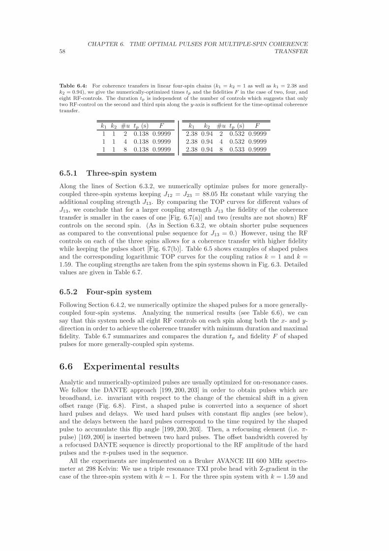
58CHAPTER 6. TIME OPTIMAL PULSES FOR MULTIPLE-SPIN COHERENCE
TRANSFER
Table 6.4: For coherence transfers in linear four-spin chains (k1 = k2 = 1 as well as k1 = 2.38 andk2 = 0.94), we give the numerically-optimized times tp and the fidelities F in the case of two, four, andeight RF-controls. The duration tp is independent of the number of controls which suggests that onlytwo RF-control on the second and third spin along the y-axis is sufficient for the time-optimal coherencetransfer.
k1 k2 #u tp (s) F1 1 2 0.138 0.99991 1 4 0.138 0.99991 1 8 0.138 0.9999
k1 k2 #u tp (s) F2.38 0.94 2 0.532 0.99992.38 0.94 4 0.532 0.99992.38 0.94 8 0.533 0.9999
6.5.1 Three-spin system
Along the lines of Section 6.3.2, we numerically optimize pulses for more generally-coupled three-spin systems keeping J12 = J23 = 88.05 Hz constant while varying theadditional coupling strength J13. By comparing the TOP curves for different values ofJ13, we conclude that for a larger coupling strength J13 the fidelity of the coherencetransfer is smaller in the cases of one [Fig. 6.7(a)] and two (results are not shown) RFcontrols on the second spin. (As in Section 6.3.2, we obtain shorter pulse sequencesas compared to the conventional pulse sequence for J13 = 0.) However, using the RFcontrols on each of the three spins allows for a coherence transfer with higher fidelitywhile keeping the pulses short [Fig. 6.7(b)]. Table 6.5 shows examples of shaped pulsesand the corresponding logarithmic TOP curves for the coupling ratios k = 1 and k =1.59. The coupling strengths are taken from the spin systems shown in Fig. 6.3. Detailedvalues are given in Table 6.7.
6.5.2 Four-spin system
Following Section 6.4.2, we numerically optimize the shaped pulses for a more generally-coupled four-spin systems. Analyzing the numerical results (see Table 6.6), we cansay that this system needs all eight RF controls on each spin along both the x- and y-direction in order to achieve the coherence transfer with minimum duration and maximalfidelity. Table 6.7 summarizes and compares the duration tp and fidelity F of shapedpulses for more generally-coupled spin systems.
6.6 Experimental results
Analytic and numerically-optimized pulses are usually optimized for on-resonance cases.We follow the DANTE approach [199, 200, 203] in order to obtain pulses which arebroadband, i.e. invariant with respect to the change of the chemical shift in a givenoffset range (Fig. 6.8). First, a shaped pulse is converted into a sequence of shorthard pulses and delays. We used hard pulses with constant flip angles (see below),and the delays between the hard pulses correspond to the time required by the shapedpulse to accumulate this flip angle [199, 200, 203]. Then, a refocusing element (i.e. π-pulse) [169, 200] is inserted between two hard pulses. The offset bandwidth covered bya refocused DANTE sequence is directly proportional to the RF amplitude of the hardpulses and the π-pulses used in the sequence.
All the experiments are implemented on a Bruker AVANCE III 600 MHz spectro-meter at 298 Kelvin: We use a triple resonance TXI probe head with Z-gradient in thecase of the three-spin system with k = 1. For the three spin system with k = 1.59 and
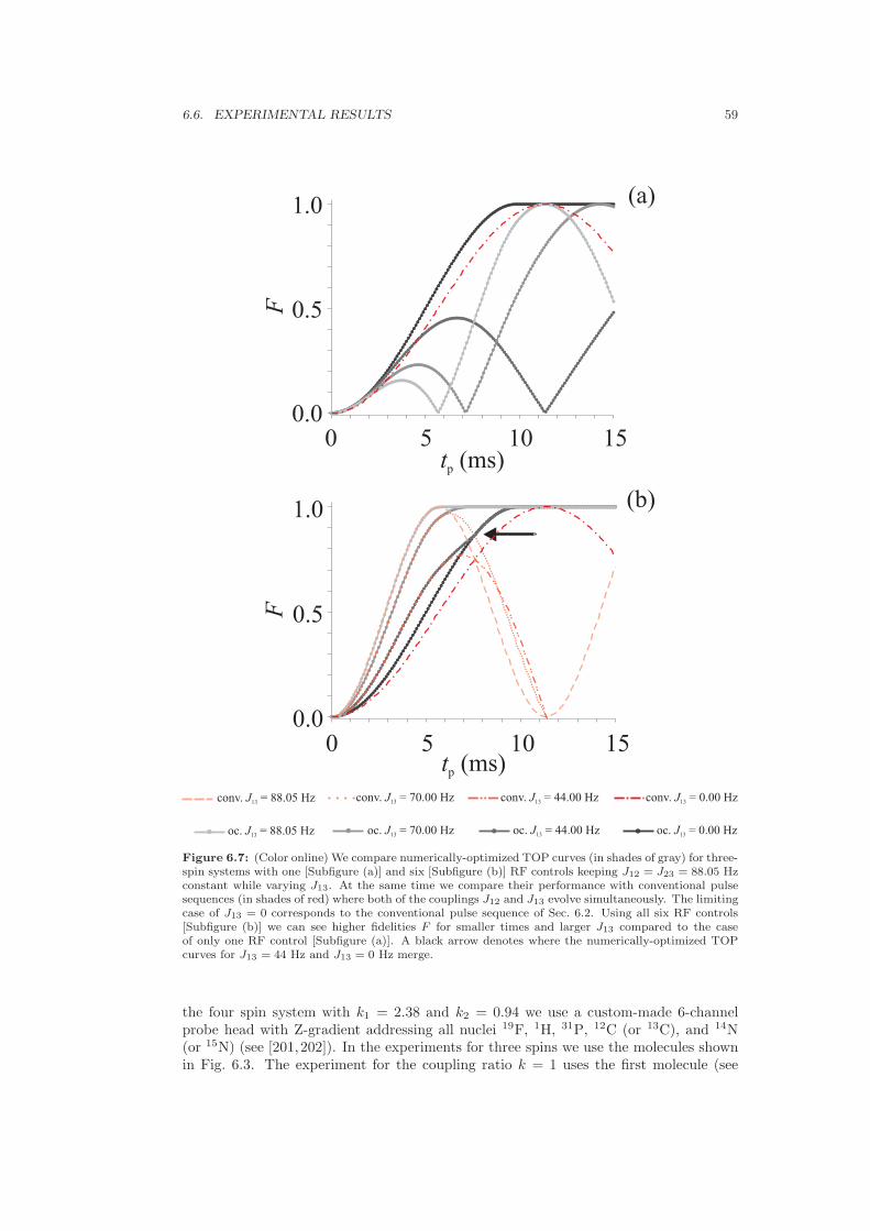
6.6. EXPERIMENTAL RESULTS 59
tp (ms)
F
0 5 10 150.0
0.5
1.0 (a)
tp (ms)
F
0 5 10 150.0
0.5
1.0 (b)
oc. = 0.00 HzJ13oc. = 44.00 HzJ13oc. = 70.00 HzJ13oc. = 88.05 HzJ13
conv. = 88.05 HzJ13conv. = 70.00 HzJ13 conv. = 44.00 HzJ13 conv. = 0.00 HzJ13
Figure 6.7: (Color online) We compare numerically-optimized TOP curves (in shades of gray) for three-spin systems with one [Subfigure (a)] and six [Subfigure (b)] RF controls keeping J12 = J23 = 88.05 Hzconstant while varying J13. At the same time we compare their performance with conventional pulsesequences (in shades of red) where both of the couplings J12 and J13 evolve simultaneously. The limitingcase of J13 = 0 corresponds to the conventional pulse sequence of Sec. 6.2. Using all six RF controls[Subfigure (b)] we can see higher fidelities F for smaller times and larger J13 compared to the caseof only one RF control [Subfigure (a)]. A black arrow denotes where the numerically-optimized TOPcurves for J13 = 44 Hz and J13 = 0 Hz merge.
the four spin system with k1 = 2.38 and k2 = 0.94 we use a custom-made 6-channelprobe head with Z-gradient addressing all nuclei 19F, 1H, 31P, 12C (or 13C), and 14N(or 15N) (see [201,202]). In the experiments for three spins we use the molecules shownin Fig. 6.3. The experiment for the coupling ratio k = 1 uses the first molecule (see

60CHAPTER 6. TIME OPTIMAL PULSES FOR MULTIPLE-SPIN COHERENCE
TRANSFER
D1 D2 D3 D4 D5 D6
(a)
(b)
(c)
21D
21D
22D
22D
2
3D2
3D2
4D2
4D2
5D2
5D2
6D2
6D
Figure 6.8: In the DANTE approach an on-resonance shaped pulse (see (a)) is converted to a seriesof short hard pulses and delays ∆i (see (b)). Then, the pulse can be converted to a broadband pulse byinserting a refocusing element (i.e. π-pulse) represented by solid bars between two hard pulses (see (c)).
Dv (kHz)
Experiment Simulation
-1 0 1Dv (kHz)
-1 0 1
(a)
(b) (b´)
(a )´
Figure 6.9: (Color online) We compare for a three-spin system the offset (∆v) profile for ±1 kHzof the anti-phase signal (see text) resulting from a conventional pulse sequence (tp = 11.4 ms) in thecase of experiment (see (a)) and simulation (see (a´) with broadband versions of the analytic pulses(tp = 9.8 ms, see (b) and (b´)) for the case of coupling ratio k = 1 of three spins.
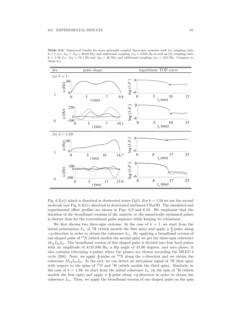
6.6. EXPERIMENTAL RESULTS 61
Table 6.5: Numerical results for more generally-coupled three-spin systems with (a) coupling ratiok = 1 (i.e. J12 = J23 = 88.05 Hz) and additional coupling J13 = 2.935 Hz as well as (b) coupling ratiok = 1.59 (i.e. J12 = 73.1 Hz and J23 = 46 Hz) and additional coupling J13 = 10.0 Hz. Compare toTable 6.1.
#u pulse shape logarithmic TOP curve
(a) k = 1:
10 3 7 9.8
0
60
t (ms)
u(H
z)
0 5 10 15-6
0
tp (ms)
log (
1-
)F
60 3 7 10.1
-1000
250
t (ms)
u(H
z)
0 5 10 15-6
0
tp (ms)lo
g (
1-
)F
(b) k = 1.59:
10 5 10 14.7
0
60
t (ms)
u(H
z)
0 8 17 25-6
0
tp (ms)
log (
1-
)F
60 5 11 15.8
-300
0100
t (ms)
u(H
z)
0 8 17 25-6
0
tp (ms)
log
(1
-)
F
Fig. 6.3(a)) which is dissolved in deuterated water D2O. For k = 1.59 we use the secondmolecule (see Fig. 6.3(b)) dissolved in deuterated methanol CD3OD. The simulated andexperimental offset profiles are shown in Figs. 6.9 and 6.10. We emphasize that theduration of the broadband versions of the analytic or the numerically-optimized pulsesis shorter than for the conventional pulse sequence while keeping its robustness.
We first discuss two three-spin systems: In the case of k = 1, we start from theinitial polarization I1z of 1H (which models the first spin) and apply a π
2 -pulse along+y-direction in order to obtain the coherence I1x. By applying a broadband version ofour shaped pulse of 15N (which models the second spin) we get the three-spin coherence4I1yI2yI3z . The broadband version of this shaped pulse is divided into four hard pulseswith an amplitude of 4145.936 Hz, a flip angle of 45.00 degrees, and zero phase; italso contains refocusing π-pulses where the phases are chosen according the MLEV-4cycle [204]. Next, we apply π
2 -pulse on 15N along the x-direction and we obtain thecoherence 4I1yI2zI3z . In the end, we can detect an anti-phase signal of 1H (first spin)with respect to the spins of 15N and 1H (which models the third spin). Similarly, inthe case of k = 1.59, we start from the initial coherence I1z on the spin of 1H (whichmodels the first spin) and apply a π
2 -pulse along +y-direction in order to obtain thecoherence I1x. Then, we apply the broadband version of our shaped pulse on the spin

62CHAPTER 6. TIME OPTIMAL PULSES FOR MULTIPLE-SPIN COHERENCE
TRANSFER
Table 6.6: Numerical results for a more generally-coupled four-spin systems with coupling ratiosk1 = 2.38 ≈ J12/J23 and k2 = 0.94 ≈ J34/J23 (i.e. J12 = 46 Hz, J23 = 19.3 Hz, and J34 = 18.1 Hz) aswell as additional couplings J13 = 4.1 Hz and J24 = 2 Hz. Compare to Table 6.3.
#u pulse shape logarithmic TOP curve
20 16 36 57.8
-400
0200
t (ms)
u(H
z)
0 20 45 70-6
0
tp (ms)
log (
1-
)F
80 16 36 54
-400
0200
t (ms)
u(H
z)
0 20 45 70-6
0
tp (ms)lo
g (
1-
)F
Dv (kHz)
Experiment Simulation
-2 -1 0 1 2Dv (kHz)
-2 -1 0 1 2
(a)
(b) (b´)
(a´)
Figure 6.10: (Color online) We compare for a three-spin system the offset (∆v) profile for ±2 kHzof the anti-phase signal (see text) resulting from a conventional pulse sequence (tp = 17.7 ms) in thecase of experiment (see (a)) and simulation (see (a´)) with broadband versions of the analytic pulses(tp = 15.5 ms, see (b) and (b´)) for the case of coupling ratio k = 1.59.
of 19F in order to produce the three-spin coherence 4I1yI2yI3z . The broadband versionof this shaped pulse is divided into four hard pulses with an amplitude of 10000 Hz, aflip angle of 45.03 degrees, and zero phase; it also contains refocusing π-pulses wherethe phases are chosen according the MLEV-4 cycle [204]. In the next step, we applya π
2 -pulse on the spin of 1H and we end up with the coherence 4I1zI2yI3z . Finally, wedetect an anti-phase signal on the spin of 19F with respect to the spins of 1H and 31P.
In the four-spin system, we show on-resonance simulations and experiments fornumerically-optimized shaped pulses comparing the conventional approach with analyt-ical and numerically-optimized pulses (see Fig. 6.11). The corresponding experimentsare implemented on the molecule of Fig. 6.6, which is dissolved in deuterated acetoni-trile. Figures 6.11(b) and (c) show a reduction in signal intensity for the simulation ifwe compare the effect of the pulse on the abstract linear spin chain (shown in gray) withthe effect on the more realistic and more generally-coupled spin system (shown in black)as the corresponding pulses were only optimized for the abstract linear spin chain. Weremark that the pulse of Fig. 6.11(d) is optimized for a more generally-coupled spinsystem while using RF-controls on all spins. Thus, we conclude—using also the data of

6.6. EXPERIMENTAL RESULTS 63
Table 6.7: We compare the duration tp and fidelity F of numerically-optimized shaped pulses in thecase of three- and four-spin systems allowing a varying number of RF controls u. Using only one RFcontrol we show the effect of indirect couplings—which are usually present in experiments—on thefidelity of optimized pulses. Hence more RF controls are necessary for higher fidelities. The J-valuesare taken from the actual spin systems shown in Figs. 6.3 and 6.6.
graph J13 (Hz) J24 (Hz) #u tp (ms) F
1 2 3
J12 J23
J13
k = 10.0 – 1 9.8 0.99992.9 – 1 9.8 0.99592.9 – 6 11.5 0.9999
k = 1.590.0 – 1 15.5 0.999910.0 – 1 15.5 0.883710.0 – 6 15.8 0.9999
1 2 3
J12 J23
4
J34
J13
J24
k1 = 2.38 and k2 = 0.940.0 0.0 2 53.2 0.99994.1 2.0 2 53.2 0.98594.1 2.0 8 54.0 0.9999
Simulation Experiment
(a)
(b)
(c)
(d)
Figure 6.11: We show the anti-phase signal of the spin of 19F with respect to the spins of 1H, 13C,and 15N of a four-spin system corresponding to the simulation (left) and experiment (right). We usethe conventional pulse sequence (a) (tp = 64.4 ms), an analytical pulse sequence (b) (tp = 53.9 ms),a pulse which was numerically-optimized for the abstract linear spin chain with RF controls on thesecond and third spin (c) (tp = 53.2 ms), and a pulse which was numerically-optimized for the moregenerally-coupled spin system with RF controls on all spins (d) (tp = 54.0 ms). The simulation for theabstract linear spin chain is given in gray color. All the other plots for the more realistic case of a moregenerally-coupled spin system are given in black color.

64CHAPTER 6. TIME OPTIMAL PULSES FOR MULTIPLE-SPIN COHERENCE
TRANSFER
0 6 12 17.550
70
t (ms)
u(H
z)
0 7 15 21.06-80
0
80
t (ms)
u(H
z)Figure 6.12: Using all ten (or twelve) RF controls we determined numerically-optimized pulse shapesfor linear spin chains of length five (or six) in the case of k = 1. We remark that most control strengthsare very small.
Table 6.7—that the pulse of Fig. 6.11(d) shows a higher fidelity when compared to thepulses of Figs. 6.11(b) and (c). Furthermore, the pulse corresponding to Fig. 6.11(d)is shorter (by 14%) than the conventional pulse sequence corresponding to Fig. 6.11(a)while maintaining its robustness to additional couplings (see also Table 6.8).
6.6.1 Conventional pulse sequences
For k = 1, the conventional pulse sequence implemented on the spectrometer is,
H1z +H2z
H90y−−−→ H1x +H2x
∆−→ H1x +H2y
90−y
−−−→ H1z +1H2y
Gz−−→ H1z (6.5)
H1z
H90y−−−→ H1x
∆1−−→ 2H1yNz
N90y−−−→ 2H1yNx
∆2−−→ 4H1yNyH1z
N90x−−−→ 4H1yNzH1z (6.6)
where, ∆ = 1/(v1 − v2), (v1 − v2) is the chemical shift difference between H1 (whichmodels the first spin) and H2 (which models the third spin), ∆1 = 1/(2JH1N ), and∆2 = 1/(2JH2N ). For k = 1.59, the conventional pulse sequence implemented on thespectrometer is,
Hz
H90y−−−→ Hx
∆1−−→ 2HyFz
H90x+F 90y
−−−−−−−→ 2HzFx∆2−−→ 4HzFyPz (6.7)
where, ∆1 = 1/(2JHF ) and ∆2 = 1/(2JFP ).
6.7 Linear spin chains with more than four spins
In this section, we generalize the numerical optimization of shaped pulses to linear spinchains of five and more spins. Figure 6.12 shows two examples of the optimized pulseshapes with coupling ratios kℓ = 1 and coupling strengths Jℓ,ℓ+1 = 88.05 Hz. Theseexamples suggest that time-optimal controls can be obtained on multiple spins evenwhile irradiating only on the spins two to ℓ − 1 along the y-direction (cp. Sec. IV ofRef. [152]). We obtain shorter pulses for the numerically-optimized pulses compared tothe conventional pulse sequences as summarized in Table 6.8.

6.8. CONCLUSION 65
Table 6.8: We compare the minimum time tp required for a coherence transfer by numerically-optimized (oc) and conventional (conv) pulse sequences for different number n of spins and couplingratios k. aFor n = 3 we have k = 1.59. And for n = 4 we have k1 = 2.38 and k2 = 0.94.
ntp (s)
k = 1 k 6= 1a
oc conv oc/conv oc conv oc/conv3 0.0098 0.0114 0.8596 0.0155 0.0177 0.87574 0.0138 0.0170 0.8118 0.0532 0.0644 0.82615 0.0177 0.0227 0.7797 – – –6 0.0216 0.0284 0.7605 – – –
6.8 Conclusion
In the case of linear three-spin chains we reproduced numerically the previous analyticalresults [151,152] obtaining the same family of restricted controls by applying pulses onlyon the second spin along the y-axis. The same holds for linear four-spin chains wherewe also obtain the analytical family of restricted controls by applying pulses only onthe second and third spin along the y-axis; but the numerically-optimized pulses appearto be a little shorter than the analytical ones. Both for three and four spins no gainin pulse duration is found if arbitrary pulse structures are allowed. These observationsare summarized in Conjectures 1 and 2. Even for longer spin chains (consisting of upto six coupled spin-1/2) there is some numerical evidence suggesting that the samerestricted controls motivated by Refs. [151,152] lead to time-optimal pulses (in the caseof unrestricted controls) for linear spin chains of arbitrary length.
Further numerical results are presented for more general and more realistic couplingtopologies, for which so far no analytical results are known. Compared to linear spinchains we obtain different pulse structures depending on the number of available controls.We hope that the presented results and conjectures will motivate further analytical workin order to develop a better understanding of time-optimal control sequences for thegeneration of multi-spin coherence.
Note that the minimum times for the transfers I1δ → 2n−1I1ǫ1 · · · Inǫn and 2n−1I1ǫ1 · · ·Inǫn → I1δ are identical (δ, ǫk ∈ {x, y, z} for k = 1, . . . , n), which is directly relevantfor “out and back” experiments and the reconversion of multiple-quantum coherence todetectable single quantum operators. In the experimental part, we demonstrated thatthe optimized pulse sequences work in realistic settings under relaxation and experi-mental imperfections (e.g. inhomogeneity of the control field, miscalibrations, and phasetransients). In addition, the pulses can be made broadband (i.e. robust with respect tofrequency offsets) using the DANTE approach.
Here we assumed for simplicity that each spin-1/2 can be selectively addressed, whichis directly relevant to heteronuclear spin systems but the optimal transfer scheme canalso be adapted to homonuclear spin systems. The presented sequences can be directlyapplied to small molecules and peptides, which is in particular true for the broadbandversions. The minimum pulse sequence durations for complete transfer are reduced byup to 24% compared to conventional approaches (see Table 6.8). Conversely, for a fixedtransfer time significantly improved transfer amplitudes are possible, e.g., for a linearthree-spin chain we gain approximately 23% in transfer efficiency when we allow only forhalf of the transfer time necessary for a complete transfer (cp. Fig. 6.7). For large pro-teins, further gains in efficiency are expected if relaxation-optimized pulse sequences canbe developed for the specific relaxation super operator given in the system. Although

66CHAPTER 6. TIME OPTIMAL PULSES FOR MULTIPLE-SPIN COHERENCE
TRANSFER
such sequences are beyond the scope of the present work, the results on time-optimalsequences presented here provide an important benchmark for relaxation-optimized se-quences.
Chapter 7
The Fantastic Four: A plug ‘n’play set of optimal controlpulses
7.1 Introduction
Hard rectangular pulses are the fundamental element of all multi-dimensional NMR pulsesequences. They are simple to use and extremely versatile. The transformations requiredfor multi-dimensional spectroscopy—excitation, flip-back, inversion, and refocusing—areall possible using this simplest of pulses. Moreover, the performance of a single hardpulse is approximately ideal over a reasonable range of resonance offsets (proportionalto the RF amplitude of the pulse) and variation in RF homogeneity (±10%) relevant forhigh resolution spectroscopy [205–217].
However, there is considerable room for improving pulse sequence performance. RFamplitude is limited in practice and cannot be increased to match the increased pulsebandwidth needed at higher field strengths. The problem of large chemical shift canbe solved by dividing the spectral region and performing multiple experiments. But,this is time consuming, and unstable samples can create problems. Even at lower fieldstrengths, relatively small errors produced by a single pulse can accumulate significantlyin multipulse sequences.
The use of shaped pulses that address particular limitations of hard pulses can im-prove performance [179], but complex multipulse sequences are masterpieces of timingand synchronized spin-state evolution. Replacing a given hard pulse in a sequence witha better performing, but longer, shaped pulse typically requires a nontrivial redesign ofthe pulse sequence. Additional pulses and delays are required to reestablish the timingand refocusing that achieve the goals of the original hard-pulse sequence (see Fig. 7.1).
The goal of the present work is to provide a fundamental set of better-performingpulses that can simply replace, in a one-to-one fashion, all the hard 90◦ and 180◦ pulsesin any existing NMR two-spin sequence. This includes important sequences such asHSQC, HMBC, HMQC, INADEQUATE, COSY, and NOESY, which are some of themost basic pulse sequences used for finding correlations between nuclei within a givenmolecule. Each hard pulse performs a universal rotation (UR), either 90◦ or 180◦, of allmagnetization components about a fixed axis, with an approximately ideal performanceover the bandwidth of the pulse. As a replacement for hard pulses, better-performing UR
67

68CHAPTER 7. THE FANTASTIC FOUR: A PLUG ‘N’ PLAY SET OF OPTIMAL
CONTROL PULSES
t1 t2
t1 t2
a
b
I
S
t1 t2
t1 t2
a
b
I
S
d1 d2
t1 t2
t1t2
a
b
I
S
(a)
(b)
c)(
Figure 7.1: This schematic demonstrates a simple block of hard pulses with flip angles α and β, anddelays τ1 and τ2 (Fig. (a)) in an any given pulse sequence. Hard pulses can be easily replaced byidentical duration Fanta4 pulses with corresponding flip angles (Fig. (c)) without altering the delays τ1and τ2. To accommodate long duration shaped pulses on 13C with respect to 1H hard pulses, delaysneed to be adjusted by δ1 and δ2 in order to account for the extra duration and possible J couplingevolution (Fig. (b)).

7.2. OPTIMIZATION 69
pulses therefore minimize the number of pulses needed. However, UR pulses are onlynecessary for refocusing or combined excitation/flip-back. Point-to-point (PP) pulsesare sufficient for excitation, flip-back, or inversion of a given initial state to a givenfinal state, and these can be designed more easily and with better performance for theirspecific task than UR pulses.
We used the optimal control based GRAPE algorithm [183] to design UR 90◦ and180◦, and PP 90◦ and 180◦ pulses with bandwidths and pulse length suitable for 1H and13C spectroscopy of small-to medium-sized molecules at 600 MHz, which is currentlya generally accessible and widely utilized spectrometer field strength. This results ina total of four pulses, which we whimsically refer to as Fanta4 due to the significantimprovement they provide in pulse sequence performance. All pulses are of the samelength, allowing each hard pulse in a sequence to be replaced by the corresponding URor PP pulse without any further modification of the sequence.
7.2 Optimization
For the first generation of Fanta4 pulses we consider applications to 13C and 1H ona 600 MHz spectrometer. In order to universally implement shaped pulses on anyavailable probe-head, we limit the maximum RF amplitude for 13C spins to 10 kHzand numerically optimize shaped pulses for 13C nuclei that cover 35 kHz (233.33 ppm)chemical shift bandwidth and are robust to ±10% RF inhomogeneity/miscalibration.For 1H nuclei, 18 kHz maximum RF amplitude was allowed and we optimized shapedpulses, which cover 20 kHz (33.33 ppm) chemical shift bandwidth and are robust to±15% RF inhomogeneity/miscalibration. The duration used in numerical optimizationof all shaped pulses is 1 ms. This is the minimum duration needed to optimize a UR180◦ 13C shaped pulse [189, 218] in the presence of the above mentioned constraints ofsufficient fidelity.
We know that R = 0 pulses [182] have no heteronuclear J coupling evolution duringa pulse when applied to a single spin. However, when applied simultaneously to 1Hand 13C, we have to account for J coupling evolution (e.g., Hartmann-Hahn transfer).This can be solved by optimizing shaped pulses for a coupled two spin-1/2 systemsimultaneously. However, optimization of shaped pulses for coupled two spin systemswith the mentioned constraints is computationally expensive. Details of coupled twospin-1/2 optimizations are provided in the appendix 7.7.1.
We simplify the coupled two spin-1/2 problem by approximating it as two independ-ent, non-interacting single spin-1/2 problems, each of which demands less computationpower by several orders of magnitude. We simulate their performance on a coupled twospin-1/2 system with a J coupling of 197 Hz.
For example, a PP 90◦ shaped pulse along x axis should bring magnetization alongz to -y axis. In the case of a coupled two spin system, a combination of PP 90◦ pulseon 1H and 13C should rotate e.g. initial zz magnetization to yy with a minimum ofunwanted terms, yz or zy, with maximum fidelity. The best shaped pulses which fellwithin the threshold value of fidelity were included in the Fanta4 pulse set. More detailsof Fanta4 pulse selection and simulation are given in appendix 7.7.2.
However, if only one pulse is applied to either of the spins, transverse magnetizationsof the other spin can evolve under the chemical shift Hamiltonian. This can be avoided bya “Do-Nothing” pulse, which create an effective rotation which is an arbitrary multipleof 360◦, which can be e.g. realized by two identical PP inversion pulses with a durationof 500 µs each.

70CHAPTER 7. THE FANTASTIC FOUR: A PLUG ‘N’ PLAY SET OF OPTIMAL
CONTROL PULSES
Numerical optimization were performed using the GRAPE (GRadient Ascent PulseEngineering) algorithm (Chapter 2).
7.3 Experiments
We chose the HSQC (Fig. 7.2) and HMBC (Fig. 7.3) experiments to demonstrate theimplementation of Fanta4 pulses. HSQC is widely used for recording one-bond cor-relation spectra between two heteronuclei and HMBC is mostly used for correlatingheteronuclei connected by multiple bonds, mostly 2-4 bonds. Hard pulses are replacedby corresponding Fanta4 pulses in these pulse sequences (Fig. 7.2 and Fig. 7.3). Sodiumformate and Hydroxycitronellal (Fig. 7.4 a and b) were used to test the performance ofFanta4-HSQC against conventional-HSQC and an intermediate molecule (Fig. 7.4c) froma reaction published in Ref. [219] is used to test Fanta4-HMBC against conventional-HMBC. All experiments were performed on Bruker AVANCE III 600 MHz spectrometerwith a triple resonance TXI probehead and Z-gradient at 298◦K.
7.4 Results
7.4.1 HSQC: Testing with Sodium Formate
13C-labeled Sodium formate (Fig. 7.4a), with one proton and one carbon spin, and a largeJ coupling (197 Hz), dissolved in D2O was used to check the performance of the Fanta4-HSQC sequence (Fig. 7.2 b) compared to the conventional-HSQC (Fig. 7.2a) at differentchemical shifts and RF miscalibrations. A proton excited and detected HSQC (coupledduring acquisition) gives doublet of a proton with respect to a carbon. We performed1D-HSQC experiments by changing the carrier frequency in the 13C dimension, a) withideal RF amplitude on 1H and 13C (Fig. 7.5a and b), and b) by miscalibrating the RFamplitude on 1H and 13C by -15% and -10% (Fig. 7.5c and d).
The conventional-HSQC (Fig. 7.2a) shows reduced signal intensity at a large offsetfrequencies (Fig. 7.5a). In addition to offset effect, RF inhomogeneity/miscalibration on1H and 13C pulses deteriorated the signal intensity (Fig. 7.5c). Small errors in the RFpulse accumulate during the pulse sequences are responsible for reduced signal intensitywith considerable phase errors. We performed similar experiments using Fanta4-HSQC(Fig. 7.2b). It shows consistent signal intensity over large chemical shift range with anideal RF amplitude (Fig. 7.5b) and with a miscalibrated RF amplitude (Fig. 7.5d) on 1Hand 13C compared to the relatively small robustness of conventional-HSQC. For moredetails see Figure 7.5.
7.4.2 HSQC: Testing with Hydroxycitronellal
We implemented the above sequences on a more complex molecule, Hydroxycitronellal(Fig. 7.4b). It consists of a long chain of hydrocarbons with a hydroxyl group on oneend and an aldehyde moiety at other end. Hydrocarbons resonate around 19 ppm anda carbon bonded to oxygen (aldehyde moiety) resonates at 202 ppm, which correspondsto total offset bandwidth of 27.3 kHz on a 600 MHz spectrometer. The conventional-HSQC experiment with an ideal RF amplitude is unable to excite the 13C nuclei at verylarge offsets and resulted in a poor signal to noise ratio (S/N)(Fig. 7.6a). This task iseven more difficult when the RF amplitude is miscalibrated on both nuclei (Fig. 7.6c).The Fanta4-HSQC showed better signal to noise ratios at large offsets both with ideal

7.4. RESULTS 71
1H
13C
G1 G2
GZ
y
f1
f2
f3
d
f3
y
f4
d1
frecD D D DD1 D1
t1
(a)
d1
d
Conventional-HSQC
UR 90o
PP 90o
UR 180o
PP 180o
Hard rectangle 90 pulseo
Hard rectangle 180 pulseo
1H
13C
G1
G2
GZ
y
f1
f2
f3
d
f3
y
f4
d1
frecD D D DD1D1
tr
tr
(b)
d1
dt1
Fanta4-HSQC
Figure 7.2: Proton excited and detected HSQC [220–222] experiment using conventional 90◦ and 180◦
hard pulses (conventional-HSQC, Fig. (a)) and Fanta4 pulses (Fanta4-HSQC, Fig. (b)). Phases are xwith the exception of Φ1 = x -x, Φ2 = x x -x -x, Φ3 = x x -x -x, Φ4 = y y -y -y, Φrec = x -x -x x.Delays are ∆ = 1/(4J) for CH groups and ∆1 = 1/(8J) for all multiplicities. δ and δ1 are delays forgradients (G1 and G2) including recovery time. ‘tr’ is a time reverse shaped pulse. Both pulse sequencesare practically of identical lengths but the offset-compensated and RF robust Fanta4-HSQC provideshigher sensitivity.

72CHAPTER 7. THE FANTASTIC FOUR: A PLUG ‘N’ PLAY SET OF OPTIMAL
CONTROL PULSES
1H
13C
G1 G2
GZ
f1
t1
f2
f3
dfrec
D
(a)
1H
13C
G1 G2
GZ
f1
t1
f2
f3
dfrec
D
(b)
Conventional-HMBC
Fanta4-HMBC
Figure 7.3: Proton excited and detected HMBC experiment [223] using conventional 90◦ and 180◦
hard pulse (conventional-HMBC (Fig. (a))) and Fanat4 pulses (Fanta4-HMBC (Fig. (b))). Phases arex with the exception of Φ1 = x -x, Φ2 = x x -x -x, Φ3 = x x x x -x -x -x -x, Φrec = x -x x -x -x x -x x.Delays are ∆ = 1/2J for evolution of long range couplings. δ is delay for gradients (G1 and G2) includingrecovery time. Both pulse sequences are practically of identical lengths but the offset-compensated andRF robust Fanta4-HMBC provides higher sensitivity.
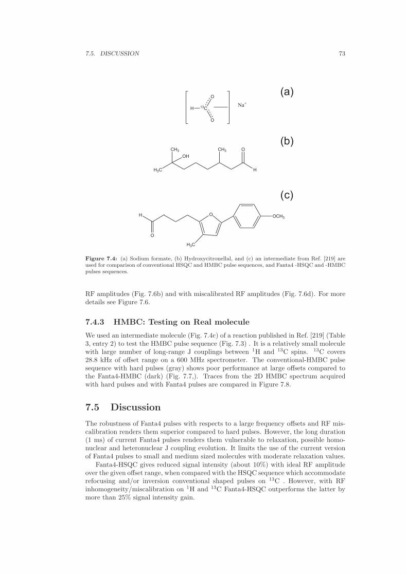
7.5. DISCUSSION 73
H
O
O OCH3
H3C
H3C H
CH3
OH
CH3 O
13C
O
O
HNa+
(a)
(b)
c)(
Figure 7.4: (a) Sodium formate, (b) Hydroxycitronellal, and (c) an intermediate from Ref. [219] areused for comparison of conventional HSQC and HMBC pulse sequences, and Fanta4 -HSQC and -HMBCpulses sequences.
RF amplitudes (Fig. 7.6b) and with miscalibrated RF amplitudes (Fig. 7.6d). For moredetails see Figure 7.6.
7.4.3 HMBC: Testing on Real molecule
We used an intermediate molecule (Fig. 7.4c) of a reaction published in Ref. [219] (Table3, entry 2) to test the HMBC pulse sequence (Fig. 7.3) . It is a relatively small moleculewith large number of long-range J couplings between 1H and 13C spins. 13C covers28.8 kHz of offset range on a 600 MHz spectrometer. The conventional-HMBC pulsesequence with hard pulses (gray) shows poor performance at large offsets compared tothe Fanta4-HMBC (dark) (Fig. 7.7,). Traces from the 2D HMBC spectrum acquiredwith hard pulses and with Fanta4 pulses are compared in Figure 7.8.
7.5 Discussion
The robustness of Fanta4 pulses with respects to a large frequency offsets and RF mis-calibration renders them superior compared to hard pulses. However, the long duration(1 ms) of current Fanta4 pulses renders them vulnerable to relaxation, possible homo-nuclear and heteronuclear J coupling evolution. It limits the use of the current versionof Fanta4 pulses to small and medium sized molecules with moderate relaxation values.
Fanta4-HSQC gives reduced signal intensity (about 10%) with ideal RF amplitudeover the given offset range, when compared with the HSQC sequence which accommodaterefocusing and/or inversion conventional shaped pulses on 13C . However, with RFinhomogeneity/miscalibration on 1H and 13C Fanta4-HSQC outperforms the latter bymore than 25% signal intensity gain.

74
CHAPTER
7.
THE
FANTASTIC
FOUR:A
PLUG
‘N’PLAY
SET
OF
OPTIM
AL
CONTROLPULSES
-17.5 -10.5 -3.5 3.5 10.5 17.5
Dn ( )kHz
-17.5 -10.5 -3.5 3.5 10.5 17.5
Dn ( )kHz
(a)
c)(
(b)
(d)
0.0
1.0
0.0
1.0
Figure 7.5: Chemical shift (∆v) excitation profile comparison of the conventional-HSQC (Fig. (a) and (c)) and the Fanta4-HSQC (Fig. (b) and (d)) acquired on a13C labeled Sodium formate dissolved in D2O. HSQC (coupled during acquisition) gives doublet of a proton with respect to a carbon. Figures (a) and (b) comparesignal intensity at different 13C resonance offsets with ideal RF amplitude, and Figures (c) and (d) show the effect of RF inhomogeneity/miscalibration for 1H(-15%) and 13C (-10%) pulses for different 13C offsets. In conventional-HSQC, the ideal RF amplitude on 1H pulses was 29.59 kHz and 13C pulses was 19.53 kHz.In case of Fanta4-HSQC, shaped pulses on 1H had a maximum amplitude of 18 kHz, while on 13C 10 kHz.

7.5.
DISCUSSIO
N75
d(1H) ppm 0.09.7
201.2
50.6
19.2
d(13
C) ppm(a) (b) (d)(c)
Figure 7.6: 2D HSQC projection acquired on 13C natural abundant Hydroxycitronellal, dissolved in deuterated tetrahydrofuran, using conventional (Fig. (a) and(c)) and Fanta4 (Fig. (b) and (d)) -HSQC. Figure (a) shows the loss in signal intensity at edge of the 13C dimension compared to Fig. (b) with ideal RF amplitude.It is worst in case of -15% RF miscalibration on 1H and -10% on 13C pulses (compare Fig. (c) and (d)). Amplitude on 1H pulses was 29 kHz and 13C pulses was19.53 kHz in conventional-HSQC. While Fanta4 pulses were with 18 kHz and 10 kHz on 1H and 13C respectively. Peaks in 1H and 13C dimension are shifted forclear distinction. Their lower and upper limits are mentioned in a plot. 1024 × 256 data points were acquired with corresponding spectral widths of 201.2 ppm(13C) and 9.7 ppm (1H). The carrier frequency on 1H was 4.5 ppm and on 13C was 100 ppm. Two transients per increment gave an overall experiment time of 25min for each of the two experiments.

76CHAPTER 7. THE FANTASTIC FOUR: A PLUG ‘N’ PLAY SET OF OPTIMAL
CONTROL PULSES
8 6 4 d ( H) ppm1
200
150
100
50
10
d ( C)ppm
13
Fanta4
hard
Figure 7.7: Amagnitude mode 2D HMBC acquired on an intermediate molecule in a reaction publishedin Ref [219], dissolved in CDCl3, is shown in the figure using conventional-HMBC (gray) and Fanta4-HMBC (black) with a slight shift in 13C dimension. The hard pulse version show loss in signal intensitycompare to Fanta4-HMBC near δ 13C = 10 to 30 ppm and at δ 13C = 202 ppm (encircled). 1024× 256data points were acquired with corresponding spectral widths of 201.2 ppm (13C) and 9.7 ppm (1H).The carrier frequency on 1H was 4.5 ppm and on 13C dimension was 100 ppm. Forty transients perincrement gave an overall experiment time of 6 hrs 25 min for each of the two experiments. For amplitudeof pulses compare Figure 7.6.

7.5. DISCUSSION 77
246810 d( H) ppm1
d( C) ppm13
202.2
21.2
106.6
Figure 7.8: (Color online) Traces through cross signals at 21.2, 106.6 and 202.2 ppm are comparedfor conventional-HMBC (red, top) and Fanta4-HMBC (black, bottom) (Fig. 7.7). The Fanta4-HMBCsequence gives improved S/N ratio compared to the conventional-HMBC sequence.

78CHAPTER 7. THE FANTASTIC FOUR: A PLUG ‘N’ PLAY SET OF OPTIMAL
CONTROL PULSES
7.6 Conclusion
We show that experimentally it is easy to replace each hard pulse with a correspond-ing Fanta4 shaped pulse without further modifying the sequence of an existing pulsesequence. The duration of the current version of Fanta4 shaped pulse is 1 ms, whichrenders them suitable for small and medium sized molecules. For Fanta4 pulses, thereis signal loss of about 10% compared to the conventional sequence on resonance dueto relaxation effects. However signal gains over large offset ranges and RF inhomogen-eity/miscalibration are substantial.
7.7 Appendix
7.7.1 Optimization of pulse pairs for two coupled heteronuclearspins-1/2
Transfer from single initial to single final state
For the optimal control problem considered here, which involves two coupled spins-1/2nuclei with defined J-coupling; with a given initial sets of product operators and finalstate, the goal is to find a RF pulse which steers the trajectory from the initial I(0)αS(0)βto the final state I(τ)γS(τ)δ . This is done by optimizing a suitably chosen cost functionΦ, where α, β, γ, and δ correspond to x, y, and z component of magnetization. The statefor the spin system is characterized by the density operator ρ(t) at time point t, andits equation of motion is the Liouville-von Neuman equation defined in Section 2.3 ofChapter 2.
Transfer from two initial to two final states
Now let us consider that the goal is to find a RF pulse which steers the trajectory of twoinitial I(0)αS(0)β and I(0)γS(0)δ to the two final states I(τ)ǫS(τ)ζ and I(τ)η S(τ)θ fora given spin system, α, β, γ, δ, ǫ, ζ, η, and θ correspond to x, y, and z components. Eachstate of the spin system is characterized by the density operator ρ1(t) and ρ2(t) at timepoint t. The Liouville-von Neuman equation for each state is given by
ρn(t) = −i[(H0 +m∑
k=1
uk(t)Hk), ρn(t)], (7.1)
where n = 1, 2, · · · , P , labels the states. The standard inner product to measure themaximum overlap of given initial states to corresponding final states is
〈Fn|ρn(T )〉 = tr{F †n ρn(T )}. (7.2)
Hence, the performance index Φn of the each transfer process can be defined as
Φn = 〈Fn|ρn(T )〉. (7.3)
and the overall performance index Φavg will be
Φavg =
P∑
n=1
Φn
P. (7.4)

7.7. APPENDIX 79
At time step j the density operators are ρ1j and ρ2j and its corresponding backwardpropagators are λ1j and λ2j . Following the steps 1. through 3. from algorithm ofSection 2.3 in Chapter 2, calculate the gradients Gnj by
Gnj =δΦn
δuk(j)= −〈λnj |i∆t[Hk, ρnj ]〉. (7.5)
and the overall gradient for all states at time j will be
Gavg(j) =
P∑
n=1
Gnj
P. (7.6)
Using Gavg(j) controls uk(j) at time step j can be improved
uk(j) → uk(j) + ǫ Gavg(j). (7.7)
Similarly we can calculate gradients for each time steps in a given control to get gradientvector over all n transfers, which later use to update the next control amplitudes.
The modified GRAPE algorithm for n number of states is
1. Guess initial controls uk(j)
2. Starting from ρn0, calculate ρnj = Uj · · ·U1 ρn0 U †1 · · ·U
†j for all j ≤ N and
n = 1, 2, · · ·P .
3. Starting from λnN = Fn, calculate λnj = U †j+1 · · ·U
†N Fn UN · · ·Uj+1 for all j ≤ N
and n = 1, 2, · · ·P .
4. Evaluate Gnj =δΦn
δuk(j)for n = 1, 2, · · ·P .
5. Evaluate Gavg(j) and update m×N control amplitudes uk(j) according to Eq. 7.7.
6. With these as the new controls, go to step 2.
The algorithm is terminated if the change in the performance index Φavg is smallerthan a chosen threshold value.
Figure 7.9 shows the shape of the pulses optimized simultaneously using above al-gorithm for 1H and 13C with J coupling of 197 Hz for the following transfers.
− IzSx → −IySx (7.8)
IzSy → −IySz (7.9)
Figure 7.10 shows the simulations for the corresponding transfers. For more details seeFigures 7.9 and 7.10.
7.7.2 Fanta4 pulse selection
A number of PP 90◦ and 180◦, and UR 90◦ and 180◦ shaped pulses are optimized for1H and 13C. Shaped pulses with fidelity ≥ 0.9999 are chosen for simulation on coupledtwo spins-1/2 system. By considering a pair of pulses in any given pulse sequence(Fig. 7.1c), we simulated the performance of all sixteen combinations of four types of 1Hwith four types of 13C shaped pulses. Simulations were performed at ideal RF amplitude
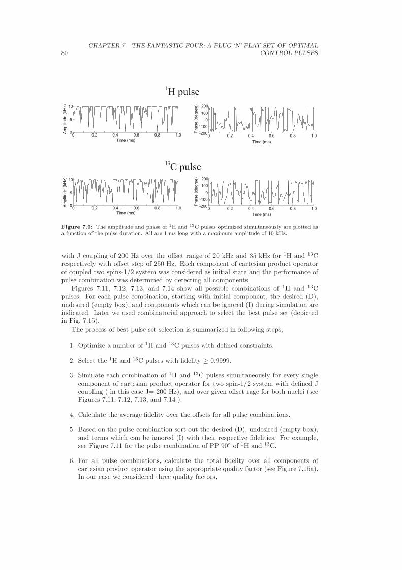
80CHAPTER 7. THE FANTASTIC FOUR: A PLUG ‘N’ PLAY SET OF OPTIMAL
CONTROL PULSES
-200
-100
0
100
200
0 0.2 0.4 0.6 0.8 1.00
5
10
0 0.2 0.4 0.6 0.8 1.0
13C pulse
0
5
10
0 0.2 0.4 0.6 0.8 1.0 -200
-100
0
100
200
0 0.2 0.4 0.6 0.8 1.0
1H pulse
Figure 7.9: The amplitude and phase of 1H and 13C pulses optimized simultaneously are plotted asa function of the pulse duration. All are 1 ms long with a maximum amplitude of 10 kHz.
with J coupling of 200 Hz over the offset range of 20 kHz and 35 kHz for 1H and 13Crespectively with offset step of 250 Hz. Each component of cartesian product operatorof coupled two spins-1/2 system was considered as initial state and the performance ofpulse combination was determined by detecting all components.
Figures 7.11, 7.12, 7.13, and 7.14 show all possible combinations of 1H and 13Cpulses. For each pulse combination, starting with initial component, the desired (D),undesired (empty box), and components which can be ignored (I) during simulation areindicated. Later we used combinatorial approach to select the best pulse set (depictedin Fig. 7.15).
The process of best pulse set selection is summarized in following steps,
1. Optimize a number of 1H and 13C pulses with defined constraints.
2. Select the 1H and 13C pulses with fidelity ≥ 0.9999.
3. Simulate each combination of 1H and 13C pulses simultaneously for every singlecomponent of cartesian product operator for two spin-1/2 system with defined Jcoupling ( in this case J= 200 Hz), and over given offset rage for both nuclei (seeFigures 7.11, 7.12, 7.13, and 7.14 ).
4. Calculate the average fidelity over the offsets for all pulse combinations.
5. Based on the pulse combination sort out the desired (D), undesired (empty box),and terms which can be ignored (I) with their respective fidelities. For example,see Figure 7.11 for the pulse combination of PP 90◦ of 1H and 13C.
6. For all pulse combinations, calculate the total fidelity over all components ofcartesian product operator using the appropriate quality factor (see Figure 7.15a).In our case we considered three quality factors,

7.7. APPENDIX 81
Figure 7.10: (Color online) Theoretical performances of 1H and 13C pulses optimized simultaneouslyfor a transfer −IzSx → −IySx and IzSy → −IySz are plotted as a function of 1H and 13C offsets.

82CHAPTER 7. THE FANTASTIC FOUR: A PLUG ‘N’ PLAY SET OF OPTIMAL
CONTROL PULSES
Q1(pc) = Min(Qd)−Max(Qud)
Q2(pc) = Min(Qd)−Max(Qud)
Q3(pc) = 1− (1−Qd2)− (0−Qud
2)
where, pc is indices for the pulse combination, Qd and Qud are the fidelities fordesired and undesired terms. Qd and Qud are averages of desired and undesiredterms. Min and Max are minimum and maximum of the values.
7. For the selected pulses with desired fidelity (Q1 or Q2 or Q3), we use the combin-atorial approach to find best set of pulses. (see Figure 7.15).
8. For every pulse set calculate fidelity Qfinal =∑
Qij , where i and j are indices forthe pulse combinations (see Figure 7.15b).
9. Choose the pulse set with highest Qfinal.
Based on this procedure the effect of heteronuclear J-coupling during shaped pulsescould be reduced by choosing appropriate pulse combination.
Q2 is summarized for the current set of 1H and 13C Fanta4 pulses in following table.
Table 7.1: Q2 is summarized for the current set of 1H and 13C Fanta4 pulses.
Q2 PPC 90◦ PPC 180◦ URC 90◦ URC 180◦
PPH 90◦ 0.4479 0.7916 0.8534 0.8497PPH 180◦ 0.8000 0.7914 0.8585 0.8606URH 90◦ 0.8831 0.8810 0.9311 0.9278URH 180◦ 0.8617 0.8716 0.9311 0.9400
7.7.3 Fanta4 pulse shapes and excitation profiles
All experiments were implemented on a Bruker 600 MHz AVANCE III spectromterequipped with SGU units for RF control and linearized amplifiers, utilizing a triple-resonance TXI probehead and gradients along the z-axis. Measurements are the residualHDO signal using a sample of 99.96% D2O doped with CuSO4 to a T1 relaxation time of100 ms at 298◦ K. For the 1H pulses shown in Figure 7.16, signals are obtained for offsetsbetween -11.1 kHz to 11.1 kHz in steps of 200 Hz at ideal RF amplitude with RFmax of 18kHz (Fig. 7.17). For the 13C pulses shown in Figure 7.18, signals are obtained at offsetsbetween -18.5 kHz to 18.5 kHz in steps of 200 Hz at ideal RF amplitude with RFmax of10 kHz (Fig. 7.17). To reduce the effects of RF field inhomogeneity, approximately 40 µlof sample solution was placed in a 5 mm Shigemi limited volume tube. The duration ofeach Fanta4 pulse is 1 ms.

7.7.
APPENDIX
83
x y z x y z xx xy xz yx yy yz zx zy zz
xyzxyzxxxyxzyxyyyzzxzyzz
I
PP 90 -H
OPP 90C
O
I D
I
I
I
I D
I
I
I
I
I
I
I
I
I
I
I
I
I
I
I
I
I
I
I
I
I
I
I
I
I
I D
x y z x y z xx xy xz yx yy yz zx zy zz
xyzxyzxxxyxzyxyyyzzxzyzz
I
PP 90 PP 180H C
O O-
I D
I
I
I
I
D
I
I
I
I
I
I
I
I
I
I
I
I
I
I
I
I
I
I
I
I
I
I
I
I
I
I
D
x y z x y z xx xy xz yx yy yz zx zy zz
xyzxyzxxxyxzyxyyyzzxzyzz
I
PP 90 90H C
O O- UR
I D
I
I
D
D
D
I
I
I
I
I
I
I
I
I
I
I
I
D
D
D
x y z x y z xx xy xz yx yy yz zx zy zz
xyzxyzxxxyxzyxyyyzzxzyzz
I
PP 90 180H C
O O- UR
I D
I
I
D
D
D
I
I
I
I
I
I
I
I
I
I
I
I
D
D
D
1H
13C
1 13H C
1H
13C
1 13H C
Final
Initial
Figure 7.11: (Color online) This figure shows the combinations of PPH 90◦ pulse with rest of 13C pulses. For simulation of pair of pulses on coupled two spins-1/2system, each component of cartesian product operator are considered as initial state and all components are detected. The desired(D, in red), undesired(emptybox), and terms which can be ignored (I) are indicated in each case.

84
CHAPTER
7.
THE
FANTASTIC
FOUR:A
PLUG
‘N’PLAY
SET
OF
OPTIM
AL
CONTROLPULSES
x y z x y z xx xy xz yx yy yz zx zy zz
xyzxyzxxxyxzyxyyyzzxzyzz
I
PP 180 PP 90H C
O O-
I
D
I
I
I
I D
I
I
I
I
I
I
I
I
I
I
I
I
I
I
I
I
I
I
I
I
I
I
I
I
I
I D
x y z x y z xx xy xz yx yy yz zx zy zz
xyzxyzxxxyxzyxyyyzzxzyzz
I
PP 180 PP 180H C
O O-
I
D
I
I
I
I
D
I
I
I
I
I
I
I
I
I
I
I
I
I
I
I
I
I
I
I
I
I
I
I
I
I
I
D
x y z x y z xx xy xz yx yy yz zx zy zz
xyzxyzxxxyxzyxyyyzzxzyzz
I
PP 180 90H C
O O- UR
I
D
I
I
D
D
D
I
I
I
I
I
I
I
I
I
I
I
I
D
D
D
x y z x y z xx xy xz yx yy yz zx zy zz
xyzxyzxxxyxzyxyyyzzxzyzz
I
PP 180 180H C
O O- UR
I
D
I
I
D
D
D
I
I
I
I
I
I
I
I
I
I
I
I
D
D
D
Figure 7.12: The combinations of PPH 180◦ pulse with rest of 13C pulses. Compare Figure 7.11.
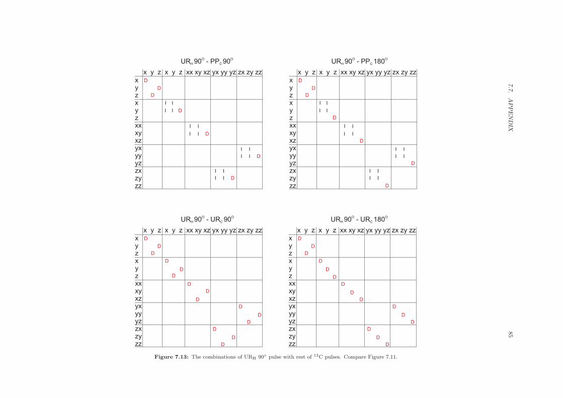
7.7.
APPENDIX
85
x y z x y z xx xy xz yx yy yz zx zy zz
xyzxyzxxxyxzyxyyyzzxzyzz
D
UR -H C90 PP 90O O
D
D
I
I D
I
I
I
I
I
I D
I
I
I
I D
I
I
I
I D
x y z x y z xx xy xz yx yy yz zx zy zz
xyzxyzxxxyxzyxyyyzzxzyzz
D
UR 90 - PP 180H C
O O
D
D
I
I
D
I
I
I
I
I
I
D
I
I
I
I
D
I
I
I
I
D
x y z x y z xx xy xz yx yy yz zx zy zz
xyzxyzxxxyxzyxyyyzzxzyzz
D
UR 90 - UR 90H C
O O
D
D
D
D
D
D
D
D
D
D
D
D
D
D
x y z x y z xx xy xz yx yy yz zx zy zz
xyzxyzxxxyxzyxyyyzzxzyzz
D
UR 90 - UR 180H C
O O
D
D
D
D
D
D
D
D
D
D
D
D
D
D
Figure 7.13: The combinations of URH 90◦ pulse with rest of 13C pulses. Compare Figure 7.11.

86
CHAPTER
7.
THE
FANTASTIC
FOUR:A
PLUG
‘N’PLAY
SET
OF
OPTIM
AL
CONTROLPULSES
x y z x y z xx xy xz yx yy yz zx zy zz
xyzxyzxxxyxzyxyyyzzxzyzz
D
UR 180 - PP 90H C
O O
D
D
I
I D
I
I
I
I
I
I D
I
I
I
I D
I
I
I
I D
x y z x y z xx xy xz yx yy yz zx zy zz
xyzxyzxxxyxzyxyyyzzxzyzz
D
UR 180 - PP 180H C
O O
D
D
I
I
D
I
I
I
I
I
I
D
I
I
I
I
D
I
I
I
I
D
x y z x y z xx xy xz yx yy yz zx zy zz
xyzxyzxxxyxzyxyyyzzxzyzz
D
UR 180 - UR 90H C
O O
D
D
D
D
D
D
D
D
D
D
D
D
D
D
x y z x y z xx xy xz yx yy yz zx zy zz
xyzxyzxxxyxzyxyyyzzxzyzz
D
UR 180 - UR 180H C
O O
D
D
D
D
D
D
D
D
D
D
D
D
D
D
Figure 7.14: The combinations of URH 180◦ pulse with rest of 13C pulses. Compare Figure 7.11.

7.7.
APPENDIX
87
PP 90H
O
PP 180H
O
UR 90H
O
UR 180H
O
PP 90C
OPP 180C
O UR 90C
OUR 180C
O
1 2 3 4 1 2 3 4 1 2 3 4 1 2 3 4
1
2
3
4
1
2
3
4
1
2
3
4
1
2
3
4
Q Q Q Q11 12 13 14
Q Q Q Q21 22 23 24
Q Q Q Q31 32 33 34
Q Q Q Q41 42 43 44
. . . .
. . . .
. . . .
. . . .
. . . .
. . . .
. . . .
. . . .
. . . .
. . . .
. . . .
. . . .
. . . .
. . . .
. . . .
. . . .
. . . .
. . . .
. . . .
. . . .
. . . .
. . . .
. . . .
. . . .
. . . .
. . . .
. . . .
. . . .
. . . .
. . . .
. . . .
. . . .
. . . .
. . . .
. . . .
. . . .
. . . .
. . . .
. . . .
. . . .
. . . .
. . . .
. . . .
. . . .
. . . .
. . . .
. . . .
. . . .
. . . .
. . . .
. . . .
. . . .
. . . .
. . . .
. . . .
. . . .
. . . .
. . . .
. . . .
. . . .
PP 90H
O
PP 180H
O
UR 90H
O
UR 180H
O
PP 90C
OPP 180C
O UR 90C
OUR 180C
O
1 1 1 11
1
1
1
. . . .
Q11Q11 Q11 Q11
Q11Q11 Q11 Q11
Q11Q11 Q11 Q11
Q11Q11 Q11 Q11
pulse set-1 pulse set-2 pulse set-3
(a)
(b)Combinatorial approach to find the best ‘pulse set’
Q (pulse set-1)final Q (pulse set-2)final Q (pulse set-3)final
. . . .
å=ijfinal
PP 90H
O
PP 180H
O
UR 90H
O
UR 180H
O
PP 90C
OPP 180C
O UR 90C
OUR 180C
O
1 1 1 21
1
1
1
Q11Q11 Q11 Q12
Q11Q11 Q11 Q12
Q11Q11 Q11 Q12
Q11Q11 Q11 Q12
PP 90H
O
PP 180H
O
UR 90H
O
UR 180H
O
PP 90C
OPP 180C
O UR 90C
OUR 180C
O
1 1 1 31
1
1
1
Q11Q11 Q11 Q13
Q11Q11 Q11 Q13
Q11Q11 Q11 Q13
Q11Q11 Q11 Q13
Figure 7.15: It depicts the combinatorial approach to select the best set of pulses. Figure (a) list the selected pulses with fidelity Qij , where i and i are indicesfor the pulse combination. Figure (b) shows the possible sets of pulses and calculation of the combined fidelity Qfinal for each pulse set.

88CHAPTER 7. THE FANTASTIC FOUR: A PLUG ‘N’ PLAY SET OF OPTIMAL
CONTROL PULSES
PP 90H
o
URH 90o
PP 18H 0o
UR 180H
o
Figure 7.16: The amplitude and phase of 1H pulses are plotted as a function of the pulse duration.All are 1 ms long with a maximum amplitude of 18 kHz.

7.7. APPENDIX 89
11.1-11.1 111 Dn ( )kHz points with 200 Hz difference
PP 90H
o
URH 90o
PP 180H
o
UR 180H
o
Figure 7.17: The experimental performance of 1H pulses is plotted as function of the offset ∆ν atideal RF amplitude with a RFmax of 18 kHz. Experiments were aquired on residual proton in HDOfor an offset range of 22.2 kHz in steps of 200 Hz. 1H pulses are optimized for 20 kHz of total offsetrange with RF miscalibration of ±5% but they are naturally robust for ±15% RF miscalibration. 1HPP 90◦ and UR 90◦ show the excitation profile for the z → −y and 1H PP 180◦ and UR 180◦ show aninversion profile from z → −z.

90CHAPTER 7. THE FANTASTIC FOUR: A PLUG ‘N’ PLAY SET OF OPTIMAL
CONTROL PULSES
PP 90C
o
URC 90o
PP 18C 0o
UR 180C
o
Figure 7.18: The amplitude and phase of 13C pulses are plotted as a function of the pulse duration.All are 1 ms long with a maximum amplitude of 10 kHz.
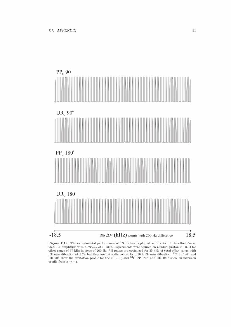
7.7. APPENDIX 91
18.5-18.5 186 Dn ( )kHz points with 200 Hz difference
PP 90C
o
URC 90o
PP 18C 0o
UR 180C
o
Figure 7.19: The experimental performance of 13C pulses is plotted as function of the offset ∆ν atideal RF amplitude with a RFmax of 10 kHz. Experiments were aquired on residual proton in HDO foroffset range of 37 kHz in steps of 200 Hz. 1H pulses are optimized for 35 kHz of total offset range withRF miscalibration of ±5% but they are naturally robust for ±10% RF miscalibration. 13C PP 90◦ andUR 90◦ show the excitation profile for the z → −y and 13C PP 180◦ and UR 180◦ show an inversionprofile from z → −z.

92CHAPTER 7. THE FANTASTIC FOUR: A PLUG ‘N’ PLAY SET OF OPTIMAL
CONTROL PULSES

Bibliography
[1] N. C. Nielsen, C. Kehlet, S. J. Glaser, and N. Khaneja. Optimal Control Methodsin NMR Spectroscopy. Encyclopedia of Nuclear Magnetic Resonance, 9:100, 2010.
[2] E. Pinch. Optimal Control and the Calculus of Variations. Oxford UniversityPress, Oxford, 1993.
[3] H. Goldstein. Classical Mechanics. Addison-Wesley, Reading, MA,, 1980.
[4] N. I. Gershenzon, K. Kobzar, B. Luy, S. J. Glaser, and T. E. Skinner. Optimal Con-trol Design of Excitation Pulses that Accomodate Relaxation. J. Magn. Reson.,188:330, 2007.
[5] T. E. Skinner, T. O. Reiss, B. Luy, N. Khaneja, and S. J. Glaser. Application ofOptimal Control Theory to the Design of Broadband Excitation Pulses for HighResolution NMR. J. Magn. Reson., 163:8, 2003.
[6] N. Khaneja, T. Reiss, C. Kehlet, T. Schulte-Herbruggen, and S. J. Glaser. OptimalControl of Coupled Spin Dynamics: Design of NMR Pulse Sequences by GradientAscent Algorithms. J. Magn. Reson., 172:296–305, 2005.
[7] N. Khaneja, T. Reiss, B. Luy, and S. J. Glaser. Optimal Control of Spin Dynamicsin the Presence of Relaxation. J. Magn. Reson., 162:311–319, 2003.
[8] N. I. Gershenzon, T. E. Skinner, B. Brutscher, N. Khaneja, M. Nimbalkar, B. Luy,and S. J. Glaser. Linear Phase Slope in Pulse Design: Application to CoherenceTransfer. J. Magn. Reson., 192:235, 2008.
[9] E. Pinch. Optimal Control and the Calculus of Variations. Oxford UniversityPress, Oxford, 1993.
[10] T. E. Skinner, T. O. Reiss, B. Luy, N. Khaneja, and S. J. Glaser. Application ofOptimal Control Theory to the Design of Broadband Excitation Pulses for HighResolution NMR. J. Magn. Reson., 163:8, 2003.
[11] T. E. Skinner, T. O. Reiss, B. Luy, N. Khaneja, and S. J. Glaser. Reducing theDuration of Broadband Excitation Pulses Using Optimal Control with LimitedRF Amplitude. J. Magn. Reson., 167:68–74, 2004.
[12] K. Kobzar, T. E. Skinner, N. Khaneja, S. J. Glaser, and B. Luy. Exploring theLimits of Broadband Excitation and Inversion Pulses. J. Magn. Reson., 170:236–243, 2004.
93

94 BIBLIOGRAPHY
[13] T. E. Skinner, T. O. Reiss, B. Luy, N. Khaneja, and S. J. Glaser. Tailoring theoptimal control cost function to a desired output: application to minimizing phaseerrors in short broadband excitation pulses. J. Magn. Reson., 172:17–23, 2005.
[14] T. E. Skinner, K. Kobzar, B. Luy, R. Bendall, W. Bermel, N. Khaneja, and S. J.Glaser. Optimal Control Design of Constant Amplitude Phase-Modulated Pulses:Application to Calibration-Free Broadband Excitation. J. Magn. Reson., 179:241,2006.
[15] Christopher Bauer, Ray Freeman, Tom Frenkiel, James Keeler, and A. J. Shaka.Gaussian pulses. J. Magn. Reson., 58:442, 1984.
[16] N. I. Gershenzon, K. Kobzar, B. Luy, S. J. Glaser, and T. E. Skinner. Optimal Con-trol Design of Excitation Pulses that Accomodate Relaxation. J. Magn. Reson.,188:330, 2007.
[17] J. S. Waugh. Theory of broadband spin decoupling. J. Magn. Reson., 50:30, 1982.
[18] E. Kupce and R. Freeman. Polychromatic selective pulses. J. Magn. Reson. Ser.A, 102:122, 1993.
[19] B. Luy, K. Kobzar, T. E. Skinner, N. Khaneja, and S. J. Glaser. Constructionof Universal Rotations from Point to Point Transformations. J. Magn. Reson.,176:179–186, 2005.
[20] Thomas E. Skinner, Naum I. Gershenzon, Manoj Nimbalkar, Wolfgang Bermel,Burkhard Luy, and Steffen J. Glaser. Broadband 180◦ universal rotation pulsesfor NMR spectroscopy designed by optimal control. J. Magn. Reson., in press,2011.
[21] M. Kock, R. Kerssebaum, and W. Bermel. A broadband ADEQUATE pulse se-quence using chirp pulses. Magn. Reson. Chem., 41:6569, 2003.
[22] M. H. Levitt and R. Freeman. NMR population inversion using a composite pulse.J. Magn. Reson., 33:473, 1979.
[23] A. J. Shaka, J. Keeler, T. Frenkiel, and R. Freeman. An improved sequence forbroadband decoupling:WALTZ-16. J. Magn. Reson., 52:335, 1983.
[24] A. J. Shaka, J. Keeler, and R. Freeman. Evaluation of a new broadband decouplingsequence: WALTZ-16. J. Magn. Reson., 53:313, 1983.
[25] J. Baum, R. Tycko, and A. Pines. Broadband population inversion by phasemodulated pulses. J. Chem. Phys., 79:4643, 1983.
[26] M. H. Levitt and R. R. Ernst. Composite pulses constructed by a recursive ex-pansion procedure. J. Magn. Reson., 55:247, 1983.
[27] M. S. Silver, R. I. Joseph, and D. I. Hoult. Selective spin inversion in nuclearmagnetic resonance and coherence optics through an exact solution of the Bloch-Riccati equation. Phys. Rev. A., 31:2753, 1985.
[28] J. Baum, R. Tycko, and A. Pines. Broadband and adiabatic inversion of a two-levelsystem by phase-modulated pulses. Phys. Rev. A., 32:3435, 1985.

BIBLIOGRAPHY 95
[29] A. J. Shaka. Composite pulses for ultra-broadband spin inversion. Phys. Lett.,120:201, 1985.
[30] M. H. Levitt. Composite pulses. Prog. Nucl. Magn. Reson. Spectrosc, 18:61122,1986.
[31] E. Kupce and R. Freeman. Adiabatic pulses for wideband inversion and broadbanddecoupling. J. Magn. Reson. Ser. A, 115:273–276, 1995.
[32] E. Kupce and R. Freeman. Optimized adiabatic pulses for wideband spin inversion.J. Magn. Reson. Ser. A, 118:299–303, 1996.
[33] A. Tannus and M. Garwood. Improved performance of frequency-swept pulsesusing offset-independent adiabaticity. J. Magn. Reson. Ser. A, 120:133–137, 1996.
[34] T. Hwang, P. van Zijl, and M. Garwood. Fast broadband inversion by adiabaticpulses. J. Magn. Reson., 133:200–203, 1998.
[35] M. A. Smith, H. Hu, and A. J. Shaka. Improved broadband inversion performancefor NMR in liquids. J. Magn. Reson., 151:269–283, 2001.
[36] K. Kobzar, T. E. Skinner, N. Khaneja, S. J. Glaser, and B. Luy. Exploring theLimits of Broadband Excitation and Inversion Pulses. J. Magn. Reson., 170:236–243, 2004.
[37] K. Kobzar, T. E. Skinner, N. Khaneja, S. J. Glaser, and B. Luy. Exploring thelimits of broadband excitation and inversion: II. Rf-power optimized pulses. J.Magn. Reson., 194:58–66, 2008.
[38] M. H. Levitt and R. Freeman. Compensation for pulse imperfections in NMRspin-echo experiments. J. Magn. Reson., 43:65–80, 1980.
[39] S. Conolly, G. Glover, D. Nishimura, and A. Macovski. A reduced power selectiveadiabatic spin-echo pulse sequence. Magn. Reson. Med., 18:28–38, 1991.
[40] T. L. Hwang, P. C. M. Van Zij, and M. Garwood. Broadband Adiabatic Refocusingwithout Phase Distortion. J. Magn. Reson., 124:250–254, 1997.
[41] B. Luy, K. Kobzar, T. E. Skinner, N. Khaneja, and S. J. Glaser. Constructionof Universal Rotations from Point to Point Transformations. J. Magn. Reson.,176:179–186, 2005.
[42] A. J. Shaka and A. J. Pines. Symmetric phase-alternating composite pulses. J.Magn. Reson., 71:495503, 1987.
[43] S. Conolly, D. Nishimura, and A. Macovski. Optimal control solutions to themagnetic resonance selective excitation problem. IEEE Trans. Med. Imaging, MI-5:106, 1986.
[44] J. Mao, T. H. Mareci, K. N. Scott, and E. R. Andrew. Selective inversion radi-ofrequency pulses by optimal control. J. Magn. Reson., 70:310318, 1986.
[45] V. Smith, J. Kurhanewicz, and T. L. James. Solvent-suppression pulses. I. Designusing optimal control theory. J. Magn. Reson., 95:4160, 1991.

96 BIBLIOGRAPHY
[46] V. Smith, J. Kurhanewicz, and T. L. James. Solvent-suppression pulses. II. In vitroand in vivo testing of optimal-control-theory pulses. J. Magn. Reson., 95:6170,1991.
[47] D. Rosenfeld and Y. Zur. Design of adiabatic selective pulses using optimal controltheory. Magn. Reson. Med., 36:401409, 1996.
[48] T. E. Skinner, T. O. Reiss, B. Luy, N. Khaneja, and S. J. Glaser. Application ofOptimal Control Theory to the Design of Broadband Excitation Pulses for HighResolution NMR. J. Magn. Reson., 163:8, 2003.
[49] T. E. Skinner, T. O. Reiss, B. Luy, N. Khaneja, and S. J. Glaser. Reducing theDuration of Broadband Excitation Pulses Using Optimal Control with LimitedRF Amplitude. J. Magn. Reson., 167:68–74, 2004.
[50] T. E. Skinner, T. O. Reiss, B. Luy, N. Khaneja, and S. J. Glaser. Tailoring theoptimal control cost function to a desired output: application to minimizing phaseerrors in short broadband excitation pulses. J. Magn. Reson., 172:17–23, 2005.
[51] T. E. Skinner, K. Kobzar, B. Luy, R. Bendall, W. Bermel, N. Khaneja, and S. J.Glaser. Optimal Control Design of Constant Amplitude Phase-Modulated Pulses:Application to Calibration-Free Broadband Excitation. J. Magn. Reson., 179:241,2006.
[52] N. I. Gershenzon, K. Kobzar, B. Luy, S. J. Glaser, and T. E. Skinner. Optimal Con-trol Design of Excitation Pulses that Accomodate Relaxation. J. Magn. Reson.,188:330, 2007.
[53] N. I. Gershenzon, T. E. Skinner, B. Brutscher, N. Khaneja, M. Nimbalkar, B. Luy,and S. J. Glaser. Linear Phase Slope in Pulse Design: Application to CoherenceTransfer. J. Magn. Reson., 192:235, 2008.
[54] N. I. Gershenzon, D. F. Miller, and T. E. Skinner. The design of excitationpulses for spin systems using optimal control theory:With application to NMRspectroscopy. Optim. Control Appl. Meth., 30:463475, 2009.
[55] N. I. Gershenzon and T. E. Skinner. Optimal control design of pulse shapes asanalytic functions. J. Magn. Reson., 204:248255, 2010.
[56] T. E. Skinner, M. Braun, K. Woelk, N. I. Gershenzon, and S. J. Glaser. Designand Application of Robust RF Pulses for Toroid Cavity NMR Spectroscopy. J.Magn. Reson., 209:282–290, 2011.
[57] N. Khaneja, T. Reiss, C. Kehlet, T. Schulte-Herbruggen, and S. J. Glaser. OptimalControl of Coupled Spin Dynamics: Design of NMR Pulse Sequences by GradientAscent Algorithms. J. Magn. Reson., 172:296–305, 2005.
[58] K. Kobzar. PhD thesis, Technische Universitat Munchen, 2007.
[59] T. W. Borneman, M. D. Hurlimann, and D. G. Cory. Application of optimalcontrol to CPMG refocusing pulse design. J. Magn. Reson., 207:220233, 2010.
[60] C. Rangan and P. H. Bucksbaum. Optimally shaped terahertz pulses for phaseretrieval in a Rydberg-atom data register. Phys. Rev. A, 64:033417–5, 2001.

BIBLIOGRAPHY 97
[61] J. P. Palao and R. Kosloff. Quantum computing by an optimal control algorithmfor unitary transformations. Phys. Rev. Lett., 89:188301–4, 2002.
[62] T. Schulte-Herbruggen, A. Sporl, and S. J. Glaser N. Khaneja. Optimal control-based efficient synthesis of building blocks of quantum algorithms seen in perspect-ive from network complexity towards time complexity. Phys. Rev. A, 72:042331–7,2005.
[63] R. P. Feynman, Jr. F. L. Vernon, and R. W. Hellwarth. Geometrical representationof the Schrodinger equation for solving maser problems. J. Appl. Phys., 28:49–52,1957.
[64] J. M. Boehlen and G. Bodenhausen. Experimental aspects of chirp NMR spectro-scopy. J. Magn. Reson. Series A, 102:293301, 1993.
[65] Thomas E. Skinner, Naum I. Gershenzon, Manoj Nimbalkar, and Steffen J. Glaser.Optimal control design of band-selective excitation pulses that accommodate re-laxation and RF inhomogeneity. J. Magn. Reson., submitted, 2011.
[66] Barrett L. Tomlinson and H. D. W. Hill. Fourier synthesized excitation of nuclearmagnetic resonance with application to homonuclear decoupling and solvent linesuppression. J. Chem. Phys., 59:17751785, 1973.
[67] Geoffrey Bodenhausen, Ray Freeman, and Gareth A. Morris. A simple pulsesequence for selective excitation in Fourier transform NMR. J. Magn. Reson.,23:171175, 1976.
[68] G. A. Morris and R. Freeman. Selective excitation in Fourier transform nuclearmagnetic resonance. J. Magn. Reson., 29:433, 1978.
[69] D. I. Hoult. The solution of the Bloch equations in the presence of a varying B1field: An approach to selective pulse analysis. J. Magn. Reson., 35:68–86, 1979.
[70] Lyndon Emsley and Geoffrey Bodenhausen. Self-refocusing effect of 270◦ Gaussianpulses. Applications to selective two-dimensional exchange spectroscopy. J. Magn.Reson., 82:211–221, 1989.
[71] P. Caravatti, G. Bodenhausen, and R. R. Ernst. Selective pulse experiments inhigh-resolution solid state NMR. J. Magn. Reson., 55:88–103, 1983.
[72] Christopher Bauer, Ray Freeman, Tom Frenkiel, James Keeler, and A. J. Shaka.Gaussian pulses. J. Magn. Reson., 58:442, 1984.
[73] D. I. Hoult M. S. Silver, R. I. Joseph. Highly selective π/2 and π pulse generation.J. Magn. Reson., 59:347–351, 1984.
[74] Jan Friedrich, Simon Davies, and Ray Freeman. Shaped selective pulses forcoherence-transfer experiments. J. Magn. Reson., 75:390–395, 1987.
[75] C. J. Hardy, P. A. Bottomley, M. O’Donnell, and P. Roemer. Optimization oftwo dimensional spatially selective NMR pulses by simulated annealing. J. Magn.Reson., 77:223–259, 1988.
[76] F. Loaiza, M. A. McCoy, S. L. Hammes, and W. S. Warren. Selective excitationwithout phase distortion using self-refocused amplitude- and amplitude/phase-modulated pulses. J. Magn. Reson., 77:175–181, 1988.

98 BIBLIOGRAPHY
[77] Piotr Tekely, Jean Brondeau, Karim Elbayed, Alain Retournard, and DanielCanet. A simple pulse train, using 90 hard pulses, for selective excitation inhigh-resolution solid-state NMR. J. Magn. Reson., 80:509–516, 1988.
[78] X.-L. Wu and R. Freeman. Darwin’s ideas applied to magnetic resonance. Themarriage broker. J. Magn. Reson., 85:414–420, 1989.
[79] H. Geen, S. Wimperis, and R. Freeman. Band-selective pulses without phasedistortion. A simulated annealing approach. J. Magn. Reson., 85:620–627, 1989.
[80] L. Emsley and G. Bodenhausen. Self-refocusing 270◦ gaussian pulses for sliceselection without gradient reversal in magnetic resonance imaging. Magn, Reson.Med., 10:273–281, 1989.
[81] A. E. Yagle. Inversion of the Bloch transform in magnetic resonance imagingusing asymmetric two-component inverse scattering. Inverse Problem, 6:133–151,1990.
[82] M. Shinnar, L. Bolinger, and J. S. Leigh. The synthesis of pulse sequences yieldingarbitrary magnetization vectors. Mag. Reson. Med., 12:74–80, 1989.
[83] M. Shinnar, L. Bolinger, and J. S. Leigh. The use of finite impulse response filtersin pulse design. Mag. Reson. Med., 12:81–87, 1989.
[84] M. Shinnar, L. Bolinger, and J. S. Leigh. The synthesis of pulse sequences yieldingarbitrary magnetization vectors. Mag. Reson. Med., 12:88–92, 1989.
[85] M. Shinnar, L. Bolinger, and J. S. Leigh. The application of spinors to pulsesynthesis and analysis. Mag. Reson. Med., 12:93–98, 1989.
[86] J. W. Carlson. Exact solution for selective-excitation pulses. Mag. Reson. Med.,94:376–386, 1991.
[87] H. Geen and R. Freeman. Band-selective radiofrequency pulses. J. Magn. Reson.,93:93–141, 1991.
[88] R. Freeman. Selective excitation in high-resolution NMR. Chem. Rev., 91-7:1397–1412, 1991.
[89] R. Freeman. High resolution NMR using selective excitation. J. Mol. Struct.,266:39–51, 1992.
[90] J. W. Carlson. Exact solution for selective-excitation pulses. II Excitation pulseswith phase control. J. Magn. Reson., 97:65, 1992.
[91] D. E. Rourke and P. G. Morris. The inverse scattering and its use in the exactinversion of the Bloch equation for noninteracting spins. J. Magn. Reson., 99:118,1992.
[92] L. Emsley and G. Bodenhausen. Optimization of shaped selective pulses for NMRusing a quaternion description of their overall propagators. J. Magn. Reson.,97:135–148, 1992.
[93] E. Kupce and R. Freeman. Polychromatic selective pulses. J. Magn. Reson. Ser.A, 102:122, 1993.

BIBLIOGRAPHY 99
[94] D. E. Rourke, M.J.W. Prior, P. G. Morris, and J. A. B. Lohman. Stereographicprojection method of exactly calculating selective pulses. J. Magn. Reson. Ser. A,107:203, 1994.
[95] L. Emsley. Selective pulses and their applications to assignment and structuredetermination in nuclear magnetic resonance. Methods Enzymol., 239:207–248,1992.
[96] E. Kupce and R. Freeman. Band-Selective Correlation Spectroscopy. J. Magn.Reson. Ser. A, 112:134–137, 1995.
[97] E. Kupce, J. Boyd, and I.D. Campbell. Short selective pulses for biochemicalapplications. J. Magn. Reson. Ser. A, 106:300–303, 1995.
[98] S. Caldarelli, A. Lesage, and L. Emsleyl. Pure-phase selective excitation in NMRby acquisition during the pulse. J. Magn. Reson. Ser. A, 116:129–132, 1995.
[99] C. Dalvit, S. Y. Ko, and J.-M. Bohlen. Single and multiple-selective excitationcombined with pulsed field gradients. J. Magn. Reson. Ser. B, 10:124–132, 1996.
[100] P. Borgnat, A. Lesage, S. Caldarelli, and L. Emsley. Narrowband linear selectivepulses for NMR. J. Magn. Reson. Ser. A, 119:289–294, 1996.
[101] E. Lunati, P. Cofrancesco, M. Villa, P. Marzola, and F. Osculati. EvolutionStrategy Optimization for Selective Pulses in NMR. J. Magn. Reson., 134:223–235,1998.
[102] A. Virgili T. Parella, F. Snchez-Ferrando. A simple approach for ultraclean multis-ite selective excitation using excitation sculpting. J. Magn. Reson., 135:50–53,1998.
[103] Ray Freeman. Shaped radiofrequency pulses in high resolution NMR. Prog. Nucl.Magn. Reson. Spectrosc., 32:59–106, 1998.
[104] P. Xu, X.-L. Wu, and R. Freeman. User-friendly selective pulses. J. Magn. Reson.,99:308–322, 1992.
[105] M. A. McCoy and L. Mueller. Nonresonant effects of frequency-selective pulses.J. Magn. Reson., 99:18–36, 1992.
[106] C. Roumestand, C. Delay, J. A. Gavid, and D. Canet. A practical approachto the implementation of selectivity in homonuclear multidimensional NMR withfrequency selective-filtering techniques. Application to the chemical structure elu-cidation of complex oligosaccharides. Magn. Reson. Chem., 37:451–478, 1999.
[107] C. Roumestand and D. Canet. Extending the excitation sculpting concept forselective excitation. J. Magn. Reson., 147:331–339, 2000.
[108] K. Zangger, M. Oberer, and H. Sterk. Pure-phase selective excitation in fast-relaxing systems. J. Magn. Reson., 152:48–56, 2001.
[109] P. Charmont, D. Sakellariou, and L. Emsley. Sample restriction using radiofre-quency field selective pulses in high-resolution solid-state NMR. J. Magn. Reson.,154:136–141, 2002.

100 BIBLIOGRAPHY
[110] K. E. Cano, M. A. Smith, and A. J. Shaka. Adjustable, broadband, selectiveexcitation with uniform phase. J. Magn. Reson., 155:131–139, 2002.
[111] M. Veshtort and R. Griffin. High-performance selective excitation pulses for solid-and liquid-state NMR spectroscopy. Chem. Phys. Chem., 5:834–850, 2004.
[112] P. J. Hajduk, D. A. Horita, and L. E. Lerner. Theoretical analysis of relaxationduring shaped pulses. The effects of short T1 and T2. J. Magn. Reson. Ser. A,103:40–52, 1993.
[113] A. Raddi and U. Klose. Relaxation effects on transverse magnetization using RFpulses long compared to T2. J. Magn. Reson., 144:108–114, 2008.
[114] J.-M. Nuzillard and R. Freeman. Band-selective pulse designed to accommodaterelaxation. J. Magn. Reson. Ser. A, 107:113–118, 1994.
[115] J. Shen and L. E. Lerner. Selective radiofrequency pulses minimizing relaxation.J. Magn. Reson. Ser. A, 112:265–1269, 1995.
[116] D. E. Rourke, L. Khodarinova, and A. A. Karabanov. Two-Level Systems withRelaxation. Phys. Rev. Letters, 92:163003–4, 2004.
[117] D. E. Rourke, A. A. Karabanov, G. H. Booth, and I. Frantsuzov. The Blochequation when T1 = T2. Inverse Problems, 23:609–623, 2007.
[118] B. Issa. Design of self-refocused pulses under short relaxation times. J. Magn.Reson., 198:151–159, 2009.
[119] Navin Khaneja, Roger Brockett, and Steffen J. Glaser. Time optimal control inspin systems. Phys. Rev. A, 63(3):032308, 2001.
[120] Timo O. Reiss, Navin Khaneja, and Steffen J. Glaser. Time-optimal coherence-order-selective transfer of in-phase coherence in heteronuclear is spin systems. J.Magn. Reson., 154(2):192–195, 2002.
[121] N. Khaneja, T. Reiss, B. Luy, and S. J. Glaser. Optimal Control of Spin Dynamicsin the Presence of Relaxation. J. Magn. Reson., 162:311–319, 2003.
[122] K. Kobzar, T. E. Skinner, N. Khaneja, S. J. Glaser, and B. Luy. Exploring theLimits of Broadband Excitation and Inversion Pulses. J. Magn. Reson., 170:236–243, 2004.
[123] K. Kobzar, B. Luy, N. Khaneja, and S. J. Glaser. Pattern Pulses: Design ofArbitrary Excitation Profiles as a Function of Pulse Amplitude and Offset. J.Magn. Reson., 173:229–235, 2005.
[124] J. L. Neves, B. Heitmann, T. O. Reiss, H. H. R. Schor, N. Khaneja, and S. J.Glaser. Exploring the Limits of Polarization Transfer Efficiency in HomonuclearThree Spin Systems. J. Magn. Reson., 181:126–134, 2006.
[125] K. Kobzar, T. E. Skinner, N. Khaneja, S. J. Glaser, and B. Luy. Exploring thelimits of broadband excitation and inversion: II. Rf-power optimized pulses. J.Magn. Reson., 194:58–66, 2008.
[126] J. L. Neves, B. Heitmann, N. Khaneja, and S. J. Glaser. Heteronuclear decouplingby optimal tracking. J. Magn. Reson., 201:7–17, 2009.

BIBLIOGRAPHY 101
[127] M. Braun and S. J. Glaser. Cooperative Pulses. J. Magn. Reson., 207:114–123,2010.
[128] N. Pomplun and S. J. Glaser. Exploring the Limits of Electron-Nuclear Polar-ization Transfer Efficiency in Three-Spin Systems. Phys. Chem. Chem. Phys.,12:5791–5798, 2010.
[129] Y. Zhang, M. Lapert, D. Sugny, M. Braun, and S. J. Glaser. Time-Optimal Controlof Spin 1/2 Particles in the Presence of Radiation Damping and Relaxation. J.Chem. Phys., 134:054103, 2011.
[130] T. E. Skinner, N. I. Gershenzon, B. Luy, and S. J. Glaser. Optimal control ofband-selective excitation pulses to accommodate relaxation, 48th ExperimentalNMR Conference (ENC) Daytona Beach, Florida, April, 2007.
[131] N. I. Gershenzon and S. J. Glaserand T. E. Skinner. Empirical relations for thedesign of band-selective pulses using optimal control theory, 48th ExperimentalNMR Conference (ENC) Daytona Beach, Florida, April, 2007.
[132] D. J. Lurie. A systematic design procedure for selective pulses in NMR imaging.Magn. Reson. Imaging, 3:235–243, 1985.
[133] M. O’Donnell and W. J. Adams. Selective time-reversal pulses for NMR imaging.Magn. Reson. Imaging, 3:377–382, 1985.
[134] J. B. Murdoch, A. H. Lent, and M. R. Kritzer. Computer-optimized narrowbandpulses for multi-slice imaging. J. Magn. Reson., 74:226–263, 1987.
[135] D. Rosenfeld and S. L. Panfil andY. Zur. Optimization of adiabatic selective pulses.J. Magn. Reson., 126:221–228, 1997.
[136] J. Pauly, P. Le Roux, D. Nishimur, and A. Macovski. Parameter relations for theShinnar-Le Roux selective excitation pulse design algorithm. IEEE Trans. Med.Imaging, 10:53, 1991.
[137] A. Hennig R. F. Schulte, J. Tsao, P. Boesiger, and K.P.Pruessmann. Design ofbroadband RF pulses with polynomial-phase response. J. Magn. Reson., 186:167–175, 2007.
[138] R. F. Schulte, P. Le Roux, M. W. Vogel, and H. Koenig. Design of phase-modulatedbroadband refocusing pulses. J. Magn. Reson., 190:271–279, 2008.
[139] T. W. Parks and C. S. Burrus. Digital Filter Design. John Wiley and Sons, NewYork, 1987.
[140] Manoj Nimbalkar, Robert Zeier, Jorge Neves, S. Begam Elavarasi, Kavita Dorai,Haidong Yuan, Navin Khaneja, and Steffen J. Glaser. Multiple-spin coherencetransfer in linear Ising spin chains and beyond: numerically-optimized pulses andexperiments. Phys. Rev. A, in press, 2011.
[141] E. Lieb, T. Schultz, and D. Mattis. Two Soluble Models of an AntiferromagneticChain. Ann. Phys., 18:407–466, 1961.
[142] H. M. Pastawski, G. Usaj, and P. R. Levstein. Quantum Interference Phenomenain the Local Polarization Dynamics of Mesoscopic Systems: an NMR Observation.Chem. Phys. Lett., 261:329–334, 1996.

102 BIBLIOGRAPHY
[143] S. J. Glaser and G. P. Drobny. Controlled Coherence Transfer by a Multiple-StepTailored TOCSY Experiment. Chem. Phys. Lett., 181:553–559, 1991.
[144] J. Listerud, S. J. Glaser, and G. P. Drobny. Symmetry and Isotropic CoherenceTransfer. II. Three Spin Calculations Using a Young Tableaux Formulation. Mol.Phys., 78:629–658, 1993.
[145] S. J. Glaser. Coupling Topology Dependence of Polarization-Transfer Efficiencyin TOCSY and TACSY Experiments. J. Magn. Reson. A, 104:283–301, 1993.
[146] S. J. Glaser and J. J. Quant. Homonuclear and Heteronuclear Hartman-HahnTransfer in Isotropic Liquids. In W. S. Warren, editor, Advances in Magnetic andOptical Resonance, volume 19, pages 59–252. Academic Press, San Diego, 1996.
[147] R. M. White. Quantum Theory of Magnetism. Springer, Berlin, 1983.
[148] D. C. Mattis. The Theory of Magnetism I, Statistics and Dynamics. Springer,Berlin, 1988.
[149] Z. L. Madi, B. Brutscher, T. Schulte-Herbruggen, R. Bruschweiler, and R. R.Ernst. Time-resolved Observation of Spin Waves in a Linear Chain of NuclearSpins. Chem. Phys. Lett., 268:300–305, 1997.
[150] N. Khaneja and S. J. Glaser. Efficient Transfer of Coherence through Ising SpinChains. Phys. Rev. A, 66:060301(R), 2002.
[151] Haidong Yuan, Steffen J. Glaser, and Navin Khaneja. Geodesics for efficient cre-ation and propagation of order along ising spin chains. Phys. Rev. A, 76(6):012316,2007.
[152] H. Yuan, R. Zeier, and N. Khaneja. Elliptic Functions and Efficient Control ofIsing Spin Chains with Unequal Couplings. Phys. Rev. A, 77:032340, 2008.
[153] F. Yamaguchi and Y. Yamamoto. Crystal Lattice Quantum Computer. Appl.Phys. A, 68:1–8, 1999.
[154] S. G. Schirmer and P. J. Pemberton-Ross. Fast High-Fidelity Information Trans-mission through Spin-Chain Quantum Wires. Phys. Rev. A, 80:030301(R), 2009.
[155] M. L. Remerowski, S. J. Glaser, and G. P. Drobny. A Theoretical Study of Co-herence Transfer by Isotropic Mixing: Calculation of Pulse Sequence Performancefor Systems of Biological Interest. Mol. Phys., 68:1191–1218, 1989.
[156] H. L. Eaton, S. W. Fesik, S. J. Glaser, and G. P. Drobny. Time Dependence of13C-13C Magnetization Transfer in Isotropic Mixing Experiments Involving AminoAcid Spin Systems. J. Magn. Reson., 90:452–463, 1990.
[157] J. Cavanagh, W. J. Fairbrother, A. G. Palmer, and N. J. Skelton. Protein NMRSpectroscopy: Principles and Practice. Academic Press, San Diego, 1996.
[158] Richard R. Ernst, Geoffrey Bodenhausen, and Alexander Wokaun. Principlesof Nuclear Magnetic Resonance in One and Two Dimensions. Clarendon Press,Oxford, 1997. reprinted with corrections.
[159] S. J. Archer, M. Ikura, D. A. Torchia, and A. Bax. An Alternative 3D NMRTechnique for Correlating Backbone 15N with Side Chain Hβ Resonances in LargerProteins. J. Magn. Reson., 95:636–641, 1991.

BIBLIOGRAPHY 103
[160] M. Sattler, J. Schleucher, and C. Griesinger. Heteronuclear multidimensionalNMR experiments for the structure determination of proteins in solution employ-ing pulsed field gradients. Prog. NMR Spec., 34:93–158, 1999.
[161] M. H. Levitt and R. R. Ernst. Multiple-quantum Excitation and Spin TopologyFiltration in High-resolution NMR. J. Chem. Phys., 83:3297–3310, 1985.
[162] E. Ising. Beitrag zur theorie des ferromagnetismus. Z. Physik, 31:253–258, 1925.
[163] Willem J. Caspers. Spin systems. World Scientific, Singapore, 1989.
[164] G. A. Morris and R. Freeman. Enhancement of Nuclear Magnetic ResonanceSignals by Polarization Transfer. J. Am. Chem. Soc., 101:760–762, 1979.
[165] Navin Khaneja, Roger Brockett, and Steffen J. Glaser. Time optimal control inspin systems. Phys. Rev. A, 63(3):032308, 2001.
[166] Timo O. Reiss, Navin Khaneja, and Steffen J. Glaser. Time-optimal coherence-order-selective transfer of in-phase coherence in heteronuclear is spin systems. J.Magn. Reson., 154(2):192–195, 2002.
[167] Navin Khaneja, Steffen J. Glaser, and Roger Brockett. Sub-riemannian geometryand time optimal control of three spin systems: quantum gates and coherencetransfer. Phys. Rev. A, 65(3):032301, 2002.
[168] Navin Khaneja, Frank Kramer, and Steffen J. Glaser. Optimal experimentsfor maximizing coherence transfer between coupled spins. J. Magn. Reson.,173(1):116–124, 2005.
[169] Navin Khaneja, Bjorn Heitmann, Andreas Sporl, Haidong Yuan, Thomas Schulte-Herbruggen, and Steffen J. Glaser. Shortest paths for efficient control of indirectlycoupled qubits. Phys. Rev. A, 75(1):012322, 2007.
[170] R. Fisher, H. Yuan, A. Sporl, and S. Glaser. Time-Optimal Generation of ClusterStates. Phys. Rev. A, 79:042304, 2009.
[171] E. Assemat, M. Lapert, Y. Zhang, M. Braun, S. J. Glaser, and D. Sugny. Simul-taneous Time-Optimal Control of the Inversion of Two Spin 1/2 Particles. Phys.Rev. A, 82:013415, 2010.
[172] N. Khaneja, T. Reiss, B. Luy, and S. J. Glaser. Optimal Control of Spin Dynamicsin the Presence of Relaxation. J. Magn. Reson., 162:311–319, 2003.
[173] N. Khaneja, B. Luy, and S. J. Glaser. Boundary of Quantum Evolution underDecoherence. Proc. Natl. Acad. Sci. USA, 100:13162–13166, 2003.
[174] D. Stefanatos, N. Khaneja, and S. J. Glaser. Optimal Control of Coupled Spinsin Presence of Longitudinal and Transverse Relaxation. Phys. Rev. A, 69:022319,2004.
[175] D. P. Fruh, T. Ito, Jr-Shin Li, G. Wagner, S. J. Glaser, and N. Khaneja. Sensitiv-ity Enhancement in NMR of Macromolecules by Application of Optimal ControlTheory. J. Biomol. NMR, 32:23–30, 2005.
[176] D. Stefanatos, N. Khaneja, and S. J. Glaser. Relaxation Optimized Transfer ofSpin Order in Ising Chains. Phys. Rev. A, 72:062320, 2005.

104 BIBLIOGRAPHY
[177] M. Lapert, Y. Zhang, M. Braun, S. J. Glaser, and D. Sugny. Singular Extremalsfor the Time-Optimal Control of Dissipative Spin 1/2 Particles. Phys. Rev. Lett.,104:083001, 2010.
[178] N. C. Nielsen, C. Kehlet, S. J. Glaser, and N. Khaneja. Optimal Control Methodsin NMR Spectroscopy. Encyclopedia of Nuclear Magnetic Resonance, 9:100, 2010.
[179] T. E. Skinner, T. O. Reiss, B. Luy, N. Khaneja, and S. J. Glaser. Application ofOptimal Control Theory to the Design of Broadband Excitation Pulses for HighResolution NMR. J. Magn. Reson., 163:8, 2003.
[180] K. Kobzar, B. Luy, N. Khaneja, and S.J. Glaser. Pattern Pulses: Design ofArbitrary Excitation Profiles as a Function of Pulse Amplitude and Offset. J.Magn. Reson., 173:229–235, 2005.
[181] K. Kobzar, T. E. Skinner, N. Khaneja, S. J. Glaser, and B. Luy. Exploring theLimits of Excitation and Inversion Pulses II: RF-Power Optimized Pulses. J.Magn. Reson., 194:58, 2008.
[182] N. I. Gershenzon, T. E. Skinner, B. Brutscher, N. Khaneja, M. Nimbalkar, B. Luy,and S. J. Glaser. Linear Phase Slope in Pulse Design: Application to CoherenceTransfer. J. Magn. Reson., 192:235, 2008.
[183] N. Khaneja, T. Reiss, C. Kehlet, T. Schulte-Herbruggen, and S. J. Glaser. OptimalControl of Coupled Spin Dynamics: Design of NMR Pulse Sequences by GradientAscent Algorithms. J. Magn. Reson., 172:296–305, 2005.
[184] Z. Tosner, T. Vosegaard, C. T. Kehlet, N. Khaneja, S. J. Glaser, and N. C. Nielsen.Optimal Control in NMR Spectroscopy: Numerical Implementation in SIMPSON.J. Magn. Reson., 197:120–134, 2009.
[185] S. Machnes, U. Sander, S. J. Glaser, P. de Fouquieres, A. Gruslys, S. Schirmer, andT. Schulte-Herbruggen. Comparing, Optimising and Benchmarking Quantum Con-trol Algorithms in a Unifying Programming Framework. Phys. Rev. A, 84:022305,2011.
[186] P. de Fouquieres, S. G. Schirmer, S. J. Glaser, and I. Kuprov. Second OrderGradient Ascent Pulse Engineering. J. Magn. Reson., 212:241–247, 2011.
[187] A. N. Pechen and D. J. Tannor. Are there Traps in Quantum Control Landscapes?Phys. Rev. Lett., 106:120402, 2011.
[188] M. Lapert, Y. Zhang, M. Braun, S. J. Glaser, and D. Sugny. Geometric VersusNumerical Optimal Control of a Dissipative Spin 1/2 Particle. Phys. Rev. A,82:063418, 2010.
[189] K. Kobzar, T. E. Skinner, N. Khaneja, S. J. Glaser, and B. Luy. Exploring theLimits of Broadband Excitation and Inversion Pulses. J. Magn. Reson., 170:236–243, 2004.
[190] J. L. Neves, B. Heitmann, T. O. Reiss, H. H. R. Schor, N. Khaneja, and S. J.Glaser. Exploring the Limits of Polarization Transfer Efficiency in HomonuclearThree Spin Systems. J. Magn. Reson., 181:126–134, 2006.

BIBLIOGRAPHY 105
[191] Nikolas Pomplun, Bjorn Heitmann, Navin Khaneja, and Steffen Glaser. Optim-ization of electron-nuclear polarization transfer. Appl. Magn. Reson., 34:331–346,2008.
[192] N. Pomplun and S. J. Glaser. Exploring the Limits of Electron-Nuclear Polar-ization Transfer Efficiency in Three-Spin Systems. Phys. Chem. Chem. Phys.,12:5791–5798, 2010.
[193] N. I. Gershenzon, K. Kobzar, B. Luy, S. J. Glaser, and T. E. Skinner. Optimal Con-trol Design of Excitation Pulses that Accomodate Relaxation. J. Magn. Reson.,188:330, 2007.
[194] M. Lapert, Y. Zhang, S. J. Glaser, and D. Sugny. Towards the Time-OptimalControl of Dissipative Spin 1/2 Particles in Nuclear Magnetic Resonance. J. Phys.B, 44:154014, 2011.
[195] Y. Zhang, M. Lapert, D. Sugny, M. Braun, and S. J. Glaser. Time-Optimal Controlof Spin 1/2 Particles in the Presence of Radiation Damping and Relaxation. J.Chem. Phys., 134:054103, 2011.
[196] T. E. Skinner, T. O. Reiss, B. Luy, N. Khaneja, and S. J. Glaser. Reducing theDuration of Broadband Excitation Pulses Using Optimal Control with LimitedRF Amplitude. J. Magn. Reson., 167:68–74, 2004.
[197] T. E. Skinner, K. Kobzar, B. Luy, R. Bendall, W. Bermel, N. Khaneja, and S. J.Glaser. Optimal Control Design of Constant Amplitude Phase-Modulated Pulses:Application to Calibration-Free Broadband Excitation. J. Magn. Reson., 179:241,2006.
[198] T. E. Skinner, M. Braun, K. Woelk, N. I. Gershenzon, and S. J. Glaser. Designand Application of Robust RF Pulses for Toroid Cavity NMR Spectroscopy. J.Magn. Reson., 209:282–290, 2011.
[199] G. A. Morris and R. Freeman. Selective excitation in Fourier transform nuclearmagnetic resonance. J. Magn. Reson., 29:433, 1978.
[200] N. Khaneja, J.-S. Li, C. Kehlet, B. Luy, and S. J. Glaser. Broadband relaxation-optimized polarization transfer in magnetic resonance. Proc. Natl. Acad. Sci. USA,101:14742, 2004.
[201] Nikolas Pomplun. PhD thesis, Technische Universitat Munchen, 2010.
[202] R. Marx, N. Pomplun, W. Bermel, H. Zeiger, F. Engelke, A. F. Fahmy, and S. J.Glaser. Engineering of an all-heteronuclear 5-qubit NMR quantum computer. inpreparation, 2011.
[203] D. Canet, J. Brondeau, and C. Roumestand. Analytical Expressions for theDANTE Pulse Sequence. J. Magn. Reson. A, 117:103, 1995.
[204] M. H. Levitt, R. Freeman, and T. Frenkiel. Broadband heteronuclear decoupling.J. Magn. Reson., 47:328–330, 1982.
[205] R. Freeman, S. P. Kempsell, and M. H. Levitt. Radiofrequency pulse sequenceswhich compensate their own imperfections. J. Magn. Reson., 38:453–479, 1980.

106 BIBLIOGRAPHY
[206] M. H. Levitt. Symmetrical composite pulse sequences for NMR population in-version. I. Compensation of radiofrequency field inhomogeneity. J. Magn. Reson.,48:234264, 1982.
[207] M. H. Levitta and R. R. Ernst. Composite pulses constructed by a recursiveexpansion procedure. J. Magn. Reson., 55:247254, 1983.
[208] R. Tycko, H.M. Cho, E. Schneider, and A. Pines. Composite pulses without phasedistortion. J. Magn. Reson., 61:9091, 1985.
[209] M. H. Levitt. Composite pulses. Prog. Nucl. Magn. Reson. Spectrosc, 18:61122,1986.
[210] A. J. Shaka and A. J. Pines. Symmetric phase-alternating composite pulses. J.Magn. Reson., 71:495503, 1987.
[211] J. M. Boehlen, M. Rey, and G. Bodenhausen. Refocusing with chirped pulses forbroadband excitation without phase dispersion. J. Magn. Reson., 84:191197, 1989.
[212] J. M. Boehlen and G. Bodenhausen. Experimental aspects of chirp NMR spectro-scopy. J. Magn. Reson. Series A, 102:293301, 1993.
[213] D. Abramovich and S. Vega. Derivation of broadband and narrowband excitationpulses using the Floquet Formalism. J. Magn. Reson. Series A, 105:30–48, 1993.
[214] E. Kupce and R. Freeman. Wideband excitation with polychromatic pulses. J.Magn. Reson. Series A, 108:268–273, 1994.
[215] K. Hallenga and G. M. Lippens. A constant-time 13C–1H HSQC with uniformexcitation over the complete 13C chemical shift range. J. Biomol. NMR, 5:59–66,1995.
[216] T. L. Hwang, P. C. M. van Zijl, and M. Garwood. Broadband adiabatic refocusingwithout phase distortion. J. Magn. Reson., 124:250–254, 1997.
[217] K. E. Cano, M. A. Smith, and A. J. Shaka. Adjustable, broadband, selectiveexcitation with uniform phase. J. Magn. Reson., 155:131–139, 2002.
[218] B. Luy, K. Kobzar, T. E. Skinner, N. Khaneja, and S. J. Glaser. Constructionof Universal Rotations from Point to Point Transformations. J. Magn. Reson.,176:179–186, 2005.
[219] Klaus-Daniel Umland, Adeline Palisse, Timm T. Haug, and Stefan F. Kirsch. Dom-ino Reactions Consisting of Heterocyclization and 1,2-MigrationRedox-Neutraland Oxidative Transition-Metal Catalysis. Angew. Chem. Int. Ed., 50:1–5, 2011.
[220] Arthur G. Palmer III, John Cavanagh, Peter E. Wright, and Mark Rance. Sens-itivity improvement in proton-detected two-dimensional heteronuclear correlationNMR spectroscopy. J. Magn. Reson., 93:151–170, 1991.
[221] J. Schleucher, M. Schwendinger, M. Sattler, P. Schmidt, O. Schedletzky, S. J.Glaser, O. W. Sørensen, and C. Griesinger. A general enhancement scheme inheteronuclear multidimensional NMR employing pulsed field gradients. J. Biomol.NMR, 4:301–306, 1994.

BIBLIOGRAPHY 107
[222] Lewis E. Kay, Paul Keifer, and Tim Saarinen. Pure absorption gradient enhancedheteronuclear single quantum correlation spectroscopy with improved sensitivity.J. Am. Chem. Soc., 114:10663–5, 1992.
[223] Daniel O. Cicero, Gaetano Barbato, and Renzo Bazzo. Sensitivity Enhancementof a Two-Dimensional Experiment for the Measurement of Heteronuclear Long-Range Coupling Constants, by a New Scheme of Coherence Selection by Gradients.J. Magn. Reson., 148:209–213, 2001.