Creating R Packages - A Tutorial

7/28/2019 Creating R Packages - A Tutorial

http://slidepdf.com/reader/full/creating-r-packages-a-tutorial 1/19

Creating R Packages: A Tutorial

Friedrich Leisch

Department of Statistics, Ludwig-Maximilians-Universitat Munchen, andR Development Core Team, [email protected]

September 14, 2009

This is a reprint of an article that has appeared in: Paula Brito, editor, Compstat 2008-Proceedings in Computational Statistics . Physica Verlag, Heidelberg, Germany, 2008.

Abstract

This tutorial gives a practical introduction to creating R packages. We discuss how object

oriented programming and S formulas can be used to give R code the usual look and feel,

how to start a package from a collection of R functions, and how to test the code once the

package has been created. As running example we use functions for standard linear regression

analysis which are developed from scratch.

Keywords: R packages, statistical computing, software, open source

1 Introduction

The R packaging system has been one of the key factors of the overall success of the R project (RDevelopment Core Team 2008). Packages allow for easy, transparent and cross-platform extensionof the R base system. An R package can be thought of as the software equivalent of a scientificarticle: Articles are the de facto standard to communicate scientific results, and readers expectthem to be in a certain format. In Statistics, there will typically be an introduction including aliterature review, a section with the main results, and finally some application or simulations.

But articles need not necessarily be the usual 10–40 pages communicating a novel scientific ideato the peer group, they may also serve other purposes. They may be a tutorial on a certain topic(like this paper), a survey, a review etc.. The overall format is always the same: text, formulasand figures on pages in a journal or book, or a PDF file on a web server. Contents and quality willvary immensely, as will the target audience. Some articles are intended for a world-wide audience,some only internally for a working group or institution, and some may only be for private use of a single person.

R packages are (after a short learning phase) a comfortable way to maintain collections of Rfunctions and data sets. As an article distributes scientific ideas to others, a package distributesstatistical methodology to others. Most users first see the packages of functions distributed withR or from CRAN. The package system allows many more people to contribute to R while stillenforcing some standards. But packages are also a convenient way to maintain private functionsand share them with your colleagues. I have a private package of utility function, my working grouphas several “experimental” packages where we try out new things. This provides a transparentway of sharing code with co-workers, and the final transition from “playground” to productioncode is much easier.

But packages are not only an easy way of sharing computational methods among peers, theyalso offer many advantages from a system administration point of view. Packages can be dy-namically loaded and unloaded on runtime and hence only occupy memory when actually used.Installations and updates are fully automated and can be executed from inside or outside R. And

1



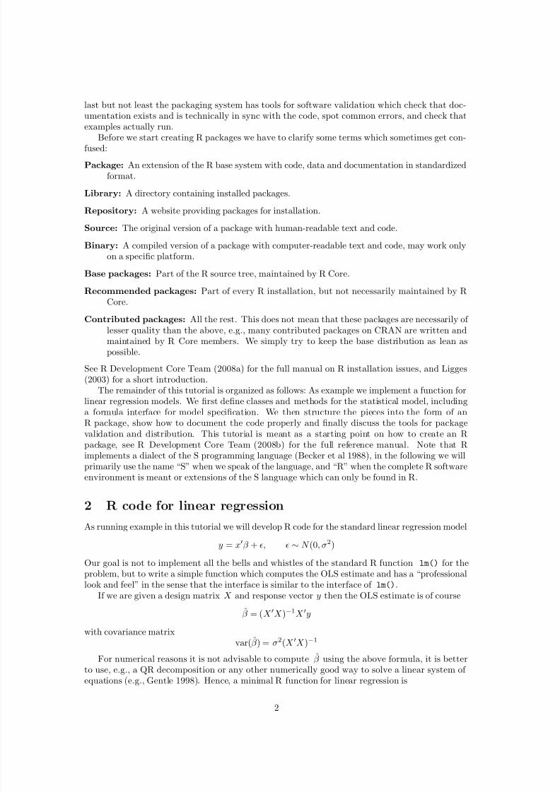
last but not least the packaging system has tools for software validation which check that doc-umentation exists and is technically in sync with the code, spot common errors, and check thatexamples actually run.

Before we start creating R packages we have to clarify some terms which sometimes get con-fused:

Package: An extension of the R base system with code, data and documentation in standardizedformat.

Library: A directory containing installed packages.

Repository: A website providing packages for installation.

Source: The original version of a package with human-readable text and code.

Binary: A compiled version of a package with computer-readable text and code, may work onlyon a specific platform.

Base packages: Part of the R source tree, maintained by R Core.Recommended packages: Part of every R installation, but not necessarily maintained by R

Core.

Contributed packages: All the rest. This does not mean that these packages are necessarily of lesser quality than the above, e.g., many contributed packages on CRAN are written andmaintained by R Core members. We simply try to keep the base distribution as lean aspossible.

See R Development Core Team (2008a) for the full manual on R installation issues, and Ligges(2003) for a short introduction.

The remainder of this tutorial is organized as follows: As example we implement a function forlinear regression models. We first define classes and methods for the statistical model, including

a formula interface for model specification. We then structure the pieces into the form of anR package, show how to document the code properly and finally discuss the tools for packagevalidation and distribution. This tutorial is meant as a starting point on how to create an Rpackage, see R Development Core Team (2008b) for the full reference manual. Note that Rimplements a dialect of the S programming language (Becker et al 1988), in the following we willprimarily use the name “S” when we speak of the language, and “R” when the complete R softwareenvironment is meant or extensions of the S language which can only be found in R.

2 R code for linear regression

As running example in this tutorial we will develop R code for the standard linear regression model

y = xβ + , ∼ N (0, σ2)

Our goal is not to implement all the bells and whistles of the standard R function lm() for theproblem, but to write a simple function which computes the OLS estimate and has a “professionallook and feel” in the sense that the interface is similar to the interface of lm().

If we are given a design matrix X and response vector y then the OLS estimate is of course

β = (X X )−1X y

with covariance matrixvar(β ) = σ2(X X )−1

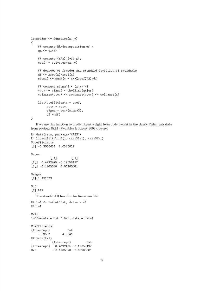
For numerical reasons it is not advisable to compute β using the above formula, it is betterto use, e.g., a QR decomposition or any other numerically good way to solve a linear system of equations (e.g., Gentle 1998). Hence, a minimal R function for linear regression is

2



linmodEst <- function(x, y)

{

## compute QR-decomposition of x

qx <- qr(x)

## compute (x’x)^(-1) x’y

coef <- solve.qr(qx, y)

## degrees of freedom and standard deviation of residuals

df <- nrow(x)-ncol(x)

sigma2 <- sum((y - x%*%coef)^2)/df

## compute sigma^2 * (x’x)^-1

vcov <- sigma2 * chol2inv(qx$qr)

colnames(vcov) <- rownames(vcov) <- colnames(x)

list(coefficients = coef,vcov = vcov,

sigma = sqrt(sigma2),

df = df)

}

If we use this function to predict heart weight from body weight in the classic Fisher cats datafrom package MASS (Venables & Ripley 2002), we get

R> data(cats, package="MASS")

R> linmodEst(cbind(1, cats$Bwt), cats$Hwt)

$coefficients

[1] -0.3566624 4.0340627

$vcov

[,1] [,2]

[1,] 0.4792475 -0.17058197

[2,] -0.1705820 0.06263081

$sigma

[1] 1.452373

$df

[1] 142

The standard R function for linear models:

R> lm1 <- lm(Hwt~Bwt, data=cats)

R> lm1

Call:

lm(formula = Hwt ~ Bwt, data = cats)

Coefficients:

(Intercept) Bwt

-0.3567 4.0341

R> vcov(lm1)

(Intercept) Bwt

(Intercept) 0.4792475 -0.17058197

Bwt -0.1705820 0.06263081

3



The numerical estimates are exactly the same, but our code lacks a convenient user interface:

1. Prettier formatting of results.

2. Add utilities for fitted model like a summary() function to test for significance of parameters.

3. Handle categorical predictors.

4. Use formulas for model specification.

Object oriented programming helps us with issues 1 and 2, formulas with 3 and 4.

3 Object oriented programming in R

3.1 S3 and S4

Our function linmodEst returns a list with four named elements, the parameter estimates andtheir covariance matrix, and the standard deviation and degrees of freedom of the residuals. From

the context it is clear to us that this is a linear model fit, however, nobody told the computer sofar. For the computer this is simply a list containing a vector, a matrix and two scalar values.Many programming languages, including S, use so-called

1. classes to define how objects of a certain type look like, and

2. methods to define special functions operating on objects of a certain class

A class defines how an object is represented in the program, while an object is an instance of theclass that exists at run time. In our case we will shortly define a class for linear model fits. Theclass is the abstract definition, while every time we actually use it to store the results for a givendata set, we create an object of the class.

Once the classes are defined we probably want to perform some computations on ob jects. Inmost cases we do not care how the object is stored internally, the computer should decide how to

perform the tasks. The S way of reaching this goal is to use generic functions and method dispatch :the same function performs different computations depending on the classes of its arguments.

S is rare because it is both interactive and has a system for ob ject-orientation. Designingclasses clearly is programming, yet to make S useful as an interactive data analysis environment,it makes sense that it is a functional language. In “real” object-oriented programming (OOP)languages like C++ or Java class and method definitions are tightly bound together, methodsare part of classes (and hence objects). We want incremental and interactive additions like user-defined methods for pre-defined classes. These additions can be made at any point in time, evenon the fly at the command line prompt while we analyze a data set. S tries to make a compromisebetween object orientation and interactive use, and although compromises are never optimal withrespect to all goals they try to reach, they often work surprisingly well in practice.

The S language has two object systems, known informally as S3 and S4.

S3 objects, classes and methods have been available in R from the beginning, they are informal,yet “very interactive”. S3 was first described in the “White Book” (Chambers & Hastie1992).

S4 objects, classes and methods are much more formal and rigorous, hence “less interactive”. S4was first described in the “Green Book” (Chambers 1998). In R it is available through the

methods package, attached by default since version 1.7.0.

S4 provides formal object oriented programming within an interactive environment. It can helpa lot to write clean and consistent code, checks automatically if objects conform to class definitions,and has much more features than S3, which in turn is more a set of naming conventions than atrue OOP system, but it is sufficient for most purposes (take almost all of R as proof). BecauseS3 is much easier to learn than S4 and sufficient for our purposes, we will use it throughout thistutorial.

4



3.2 The S3 system

If we look at the following R session we already see the S3 system of classes and methods at work:

R> x <- rep(0:1, c(10, 20))R> x

[1] 0 0 0 0 0 0 0 0 0 0 1 1 1 1 1 1 1 1 1 1 1 ...

R> class(x)

[1] "integer"

R> summary(x)

Min. 1st Qu. Median Mean 3rd Qu. Max.

0.0000 0.0000 1.0000 0.6667 1.0000 1.0000

R> y <- as.factor(x)

R> class(y)

[1] "factor"

R> summary(y)

0 1

10 20

Function summary() is a generic function which performs different operations on objects of differentclasses. In S3 only the class of the first argument to a generic function counts. For objects of class "integer" (or more generally "numeric") like x the five number summary plus the mean iscalculated, for objects of class "factor" like y a table of counts.

Classes are attached to objects as an attribute:

R> attributes(y)

$levels

[1] "0" "1"

$class

[1] "factor"

In S3 there is no formal definition of a class. To create an object from a new class, one simplysets the class attribute of an object to the name of the desired class:

R> myx <- x

R> class(myx) <- "myvector"

R> class(myx)

[1] "myvector"

Of course in most cases it is useless to define a class without defining any methods for theclass, i.e., functions which do special things for objects from the class. In the simplest case onedefines new methods for already existing generic functions like print(), summary() or plot().These are available for objects of many different classes and should do the following:

print(x, ...): this method is called, when the name of an object is typed at the prompt. Fordata objects it usually shows the complete data, for fitted models a short description of themodel (only a few lines).

summary(x, ...): for data objects summary statistics, for fitted models statistics on parameters,residuals and model fit (approx. one screen). The summary method should not directly createscreen output, but return an object which is then print()ed.

plot(x, y, ...): create a plot of the object in a graphics device.

Generic functions in S3 take a look at the class of their first argument and do method dispatchbased on a naming convention: foo() methods for objects of class "bar" are called foo.bar(),

5



e.g., summary.factor() or print.myvector(). If no bar method is found, S3 searches forfoo.default(). Inheritance can be emulated by using a class vector.

Let us return to our new class called "myvector". To define a new print() method for our

class, all we have to do is define a function called print.myvector():

print.myvector <- function(x, ...){

cat("This is my vector:\n")

cat(paste(x[1:5]), "...\n")

}

If we now have a look at x and myx they are printed differently:

R> x

[1] 0 0 0 0 0 0 0 0 0 0 1 1 1 1 1 1 1 1 1 1 1 1 1 1 1 1 1 1 1 1

R> myx

This is my vector:

0 0 0 0 0 0 0 0 0 0 ...

So we see that S3 is highly interactive, one can create new classes and change methods defini-tions on the fly, and it is easy to learn. Because everything is just solved by naming conventions(which are not checked by R at runtime1), it is easy to break the rules. A simple example: Func-tion lm() returns objects of class "lm". Methods for that class of course expect a certain formatfor the objects, e.g., that they contain regression coefficients etc as the following simple exampleshows:

R> nolm <- "This is not a linear model!"

R> class(nolm) <- "lm"

R> nolm

Call:

NULL

No coefficients

Warning messages:

1: In x$call : $ operator is invalid for

atomic vectors, returning NULL

2: In object$coefficients :

$ operator is invalid for atomic vectors,

returning NULL

The computer should detect the real problem: a character string is not an "lm" object. S4 providesfacilities for solving this problem, however at the expense of a steeper learning curve.

In addition to the simple naming convention on how to find objects, there are several more

conventions which make it easier to use methods in practice:• A method must have all the arguments of the generic, including ... if the generic does.

• A method must have arguments in exactly the same order as the generic.

• If the generic specifies defaults, all methods should use the same defaults.

The reason for the above rules is that they make it less necessary to read the documentation forall methods corresponding to the same generic. The user can rely on common rules, all methodsoperate “as similar” as possible. Unfortunately there are no rules without exceptions, as we willsee in one of the next sections . . .

1There is checking done as part of package quality control, see the section on R CMD check later in this tutorial.

6



3.3 Classes and methods for linear regression

We will now define classes and methods for our linear regression example. Because we want towrite a formula interface we make our main function linmod() generic, and write a default methodwhere the first argument is a design matrix (or something which can be converted to a matrix).Later-on we will add a second method where the first argument is a formula.

A generic function is a standard R function with a special body, usually containing only a callto UseMethod:

linmod <- function(x, ...) UseMethod("linmod")

To add a default method, we define a function called linmod.default():

linmod.default <- function(x, y, ...)

{

x <- as.matrix(x)

y <- as.numeric(y)

est <- linmodEst(x, y)

est$fitted.values <- as.vector(x %*% est$coefficients)

est$residuals <- y - est$fitted.values

est$call <- match.call()

class(est) <- "linmod"

est

}

This function tries to convert its first argument x to a matrix, as.matrix() will throw an error if the conversion is not successful2, similarly for the conversion of y to a numeric vector. We then

call our function for parameter estimation, and add fitted values, residuals and the function callto the results. Finally we set the class of the return object to "linmod".Defining the print() method for our class as

print.linmod <- function(x, ...)

{

cat("Call:\n")

print(x$call)

cat("\nCoefficients:\n")

print(x$coefficients)

}

makes it almost look like the real thing:

R> x = cbind(Const=1, Bwt=cats$Bwt)R> y = cats$Hw

R> mod1 <- linmod(x, y)

R> mod1

Call:

linmod.default(x = x, y = y)

Coefficients:

Const Bwt

-0.3566624 4.0340627

2What we do not catch here is conversion to a non-numeric matrix like character strings.

7



Note that we have used the standard names "coefficients", "fitted.values" and"residuals" for the elements of our class "linmod". As a bonus on the side we get methodsfor several standard generic functions for free, because their default methods work for our class:

R> coef(mod1)

Const Bwt

-0.3566624 4.0340627

R> fitted(mod1)

[1] 7.711463 7.711463 7.711463 8.114869 8.114869 8.114869 ...

R> resid(mod1)

[1] -0.7114630 -0.3114630 1.7885370 -0.9148692 -0.8148692 ...

The notion of functions returning an object of a certain class is used extensively by the mod-elling functions of S. In many statistical packages you have to specify a lot of options controllingwhat type of output you want/need. In S you first fit the model and then have a set of methodsto investigate the results (summary tables, plots, . . . ). The parameter estimates of a statisticalmodel are typically summarized using a matrix with 4 columns: estimate, standard deviation, z

(or t or ...) score and p-value. The summary method computes this matrix:

summary.linmod <- function(object, ...)

{

se <- sqrt(diag(object$vcov))

tval <- coef(object) / se

TAB <- cbind(Estimate = coef(object),

StdErr = se,

t.value = tval,

p.value = 2*pt(-abs(tval), df=object$df))

res <- list(call=object$call,

coefficients=TAB)

class(res) <- "summary.linmod"

res

}

The utility function printCoefmat() can be used to print the matrix with appropriate roundingand some decoration:

print.summary.linmod <- function(x, ...)

{

cat("Call:\n")

print(x$call)

cat("\n")

printCoefmat(x$coefficients, P.value=TRUE, has.Pvalue=TRUE)

}

The results is

R> summary(mod1)

Call:

linmod.default(x = x, y = y)

Estimate StdErr t.value p.value

Const -0.35666 0.69228 -0.5152 0.6072

8



Bwt 4.03406 0.25026 16.1194 <2e-16 ***

---

Signif. codes: 0 *** 0.001 ** 0.01 * 0.05 . 0.1 1

Separating computation and screen output has the advantage, that we can use all values if neededfor later computations. E.g., to obtain the p-values we can use

R> coef(summary(mod1))[,4]

Const Bwt

6.072131e-01 6.969045e-34

4 S Formulas

The unifying interface for selecting variables from a data frame for a plot, test or model are Sformulas. The most common formula is of type

y ~ x1+x2+x3The central object that is usually created first from a formula is the

model.frame, a data frame containing only the variables appearing in the formula, together withan interpretation of the formula in the

terms attribute. It tells us whether there is a response variable (always the first column of the model.frame), an intercept, . . .

The model.frame is then used to build the design matrix for the model and get the response.Our code shows the simplest handling of formulas, which however is already sufficient for manyapplications (and much better than no formula interface at all):

linmod.formula <- function(formula, data=list(), ...)

{ mf <- model.frame(formula=formula, data=data)

x <- model.matrix(attr(mf, "terms"), data=mf)

y <- model.response(mf)

est <- linmod.default(x, y, ...)

est$call <- match.call()

est$formula <- formula

est

}

The above function is an example for the most common exception to the rule that all methodsshould have the same arguments as the generic and in the same order. By convention formula

methods have arguments formula and data (rather than x and y), hence there is at least adifference in names of the first argument: x in the generic, formula in the formula method. Thisexception is hard-coded in the quality control tools of R CMD check described below.

The few lines of R code above give our model access to the wide variety of design matrices Sformulas allow us to specify. E.g., to fit a model with main effects and an interaction term forbody weight and sex we can use

R> summary(linmod(Hwt~Bwt*Sex, data=cats))

Call:

linmod.formula(formula = Hwt ~ Bwt * Sex, data = cats)

Estimate StdErr t.value p.value

(Intercept) 2.98131 1.84284 1.6178 0.1079605

9



Bwt 2.63641 0 .77590 3 .3979 0.0008846 ***

SexM -4.16540 2.06176 -2.0203 0.0452578 *

Bwt:SexM 1.67626 0.83733 2.0019 0.0472246 *

---Signif. codes: 0 *** 0.001 ** 0.01 * 0.05 . 0.1 1

The last missing methods most statistical models in S have are a plot() and predict()

method. For the latter a simple solution could be

predict.linmod <- function(object, newdata=NULL, ...)

{

if(is.null(newdata))

y <- fitted(object)

else{

if(!is.null(object$formula)){

## model has been fitted using formula interface

x <- model.matrix(object$formula, newdata)

}

else{

x <- newdata

}

y <- as.vector(x %*% coef(object))

}

y

}

which works for models fitted with either the default method (in which case newdata is assumedto be a matrix with the same columns as the original x matrix), or for models fitted using theformula method (in which case newdata will be a data frame). Note that model.matrix() canalso be used directly on a formula and a data frame rather than first creating a model.frame.

The formula handling in our small example is rather minimalistic, production code usuallyhandles much more cases. We did not bother to think about treatment of missing values, weights,offsets, subsetting etc. To get an idea of more elaborate code for handling formulas, one can lookat the beginning of function lm() in R.

5 R packages

Now that we have code that does useful things and has a nice user interface, we may want to shareour code with other people, or simply make it easier to use ourselves. There are two popular waysof starting a new package:

1. Load all functions and data sets you want in the package into a clean R session, and run

package.skeleton(). The objects are sorted into data and functions, skeleton help filesare created for them using prompt() and a DESCRIPTION file is created. The function thenprints out a list of things for you to do next.

2. Create it manually, which is usually faster for experienced developers.

5.1 Structure of a package

The extracted sources of an R package are simply a directory3 somewhere on your hard drive. Thedirectory has the same name as the package and the following contents (all of which are describedin more detail below):

3Directories are sometimes also called folders, especially on Windows.

10



• A file named DESCRIPTION with descriptions of the package, author, and license conditionsin a structured text format that is readable by computers and by people.

• A man/ subdirectory of documentation files.

• An R/ subdirectory of R code.

• A data/ subdirectory of datasets.

Less commonly it contains

• A src/ subdirectory of C, Fortran or C++ source.

• tests/ for validation tests.

• exec/ for other executables (eg Perl or Java).

• inst/ for miscellaneous other stuff. The contents of this directory are completely copied tothe installed version of a package.

• A configure script to check for other required software or handle differences between sys-tems.

All but the DESCRIPTION file are optional, though any useful package will have man/ and at leastone of R/ and data/. Note that capitalization of the names of files and directories is important,R is case-sensitive as are most operating systems (except Windows).

5.2 Starting a package for linear regression

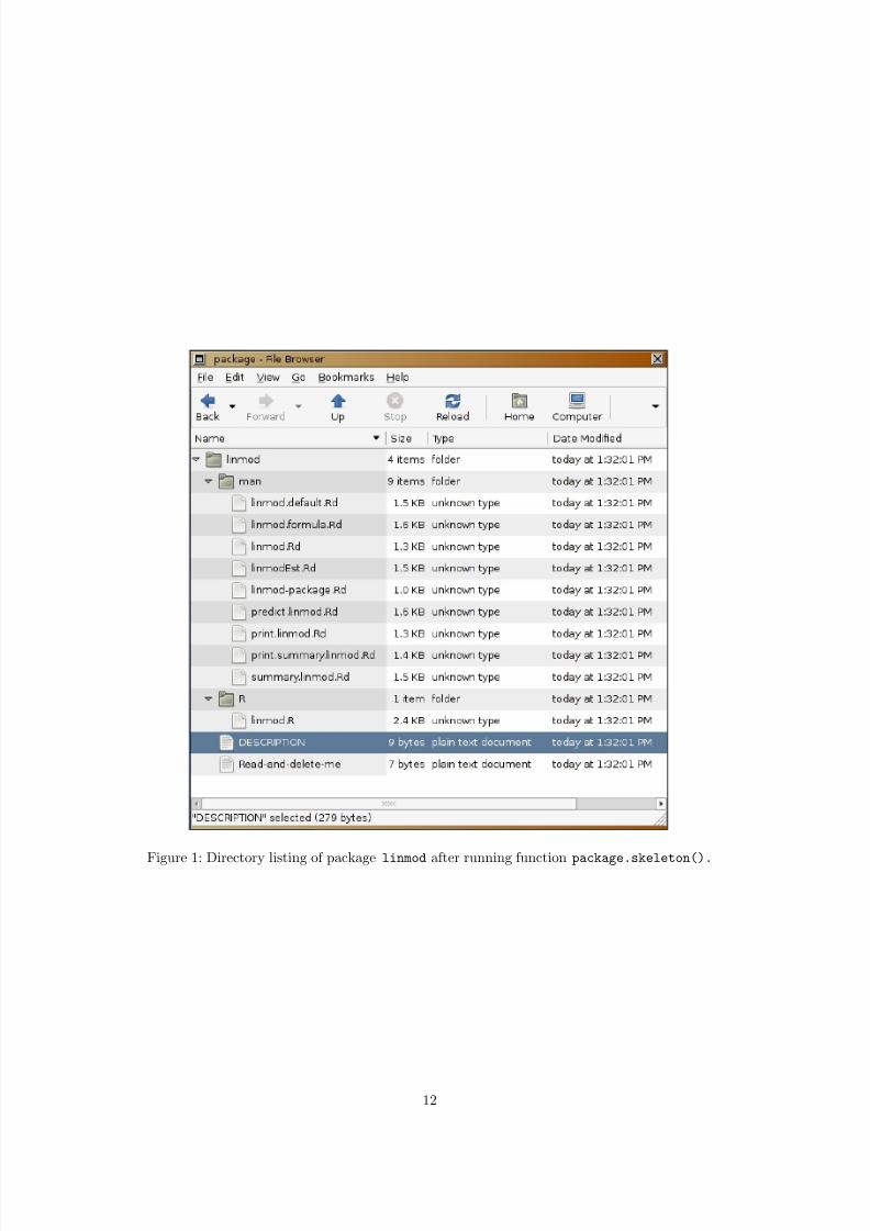
To start a package for our R code all we have to do is run function package.skeleton() andpass it the name of the package we want to create plus a list of all source code files. If no sourcefiles are given, the function will use all objects available in the user workspace. Assuming that allfunctions defined above are collected in a file called linmod.R, the corresponding call is

R> package.skeleton(name="linmod", code_files="linmod.R")Creating directories ...

Creating DESCRIPTION ...

Creating Read-and-delete-me ...

Copying code files ...

Making help files ...

Done.

Further steps are described in ’./linmod/Read-and-delete-me’.

which already tells us what to do next. It created a directory called "linmod" in the currentworking directory, a listing can be seen in Figure 1. R also created subdirectories man and R,copied the R code into subdirectory R and created stumps for help file for all functions in thecode.

File Read-and-delete-me contains further instructions:* Edit the help file skeletons in ’man’, possibly

combining help files for multiple functions.

* Put any C/C++/Fortran code in ’src’.

* If you have compiled code, add a .First.lib() function

in ’R’ to load the shared library.

* Run R CMD build to build the package tarball.

* Run R CMD check to check the package tarball.

Read "Writing R Extensions" for more information.

We do not have any C or Fortran code, so we can forget about items 2 and 3. The code is alreadyin place, so all we need to do is edit the DESCRIPTION file and write some help pages.

11



Figure 1: Directory listing of package linmod after running function package.skeleton().

12



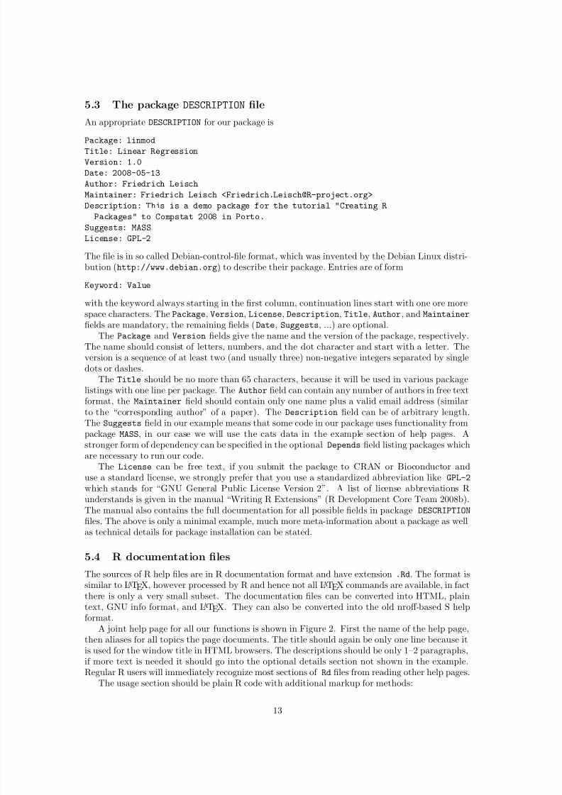
5.3 The package DESCRIPTION file

An appropriate DESCRIPTION for our package is

Package: linmodTitle: Linear Regression

Version: 1.0

Date: 2008-05-13

Author: Friedrich Leisch

Maintainer: Friedrich Leisch <[email protected]>

Description: This is a demo package for the tutorial "Creating R

Packages" to Compstat 2008 in Porto.

Suggests: MASS

License: GPL-2

The file is in so called Debian-control-file format, which was invented by the Debian Linux distri-bution (http://www.debian.org) to describe their package. Entries are of form

Keyword: Value

with the keyword always starting in the first column, continuation lines start with one ore morespace characters. The Package, Version, License, Description, Title, Author, and Maintainer

fields are mandatory, the remaining fields (Date, Suggests, ...) are optional.The Package and Version fields give the name and the version of the package, respectively.

The name should consist of letters, numbers, and the dot character and start with a letter. Theversion is a sequence of at least two (and usually three) non-negative integers separated by singledots or dashes.

The Title should be no more than 65 characters, because it will be used in various packagelistings with one line per package. The Author field can contain any number of authors in free textformat, the Maintainer field should contain only one name plus a valid email address (similarto the “corresponding author” of a paper). The Description field can be of arbitrary length.The Suggests field in our example means that some code in our package uses functionality frompackage MASS, in our case we will use the cats data in the example section of help pages. Astronger form of dependency can be specified in the optional Depends field listing packages whichare necessary to run our code.

The License can be free text, if you submit the package to CRAN or Bioconductor anduse a standard license, we strongly prefer that you use a standardized abbreviation like GPL-2

which stands for “GNU General Public License Version 2”. A list of license abbreviations Runderstands is given in the manual “Writing R Extensions” (R Development Core Team 2008b).The manual also contains the full documentation for all possible fields in package DESCRIPTION

files. The above is only a minimal example, much more meta-information about a package as wellas technical details for package installation can be stated.

5.4 R documentation filesThe sources of R help files are in R documentation format and have extension .Rd. The format issimilar to LATEX, however processed by R and hence not all LATEX commands are available, in factthere is only a very small subset. The documentation files can be converted into HTML, plaintext, GNU info format, and LATEX. They can also be converted into the old nroff-based S helpformat.

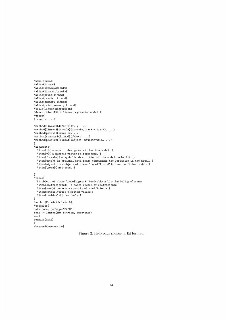
A joint help page for all our functions is shown in Figure 2. First the name of the help page,then aliases for all topics the page documents. The title should again be only one line because itis used for the window title in HTML browsers. The descriptions should be only 1–2 paragraphs,if more text is needed it should go into the optional details section not shown in the example.Regular R users will immediately recognize most sections of Rd files from reading other help pages.

The usage section should be plain R code with additional markup for methods:

13



\name{linmod}

\alias{linmod}

\alias{linmod.default}

\alias{linmod.formula}

\alias{print.linmod}

\alias{predict.linmod}

\alias{summary.linmod}

\alias{print.summary.linmod}

\title{Linear Regression}

\description{Fit a linear regression model.}\usage{

linmod(x, ...)

\method{linmod}{default}(x, y, ...)

\method{linmod}{formula}(formula, data = list(), ...)

\method{print}{linmod}(x, ...)

\method{summary}{linmod}(object, ...)

\method{predict}{linmod}(object, newdata=NULL, ...)

}

\arguments{

\item{x}{ a numeric design matrix for the model. }

\item{y}{ a numeric vector of responses. }

\item{formula}{ a symbolic description of the model to be fit. }

\item{data}{ an optional data frame containing the variables in the model. }

\item{object}{ an object of class \code{"linmod"}, i.e., a fitted model. }

\item{\dots}{ not used. }

}

\value{

An object of class \code{logreg}, basically a list including elements

\item{coefficients}{ a named vector of coefficients }

\item{vcov}{ covariance matrix of coefficients }

\item{fitted.values}{ fitted values }

\item{residuals}{ residuals }

}

\author{Friedrich Leisch}

\examples{

data(cats, package="MASS")

mod1 <- linmod(Hwt~Bwt*Sex, data=cats)

mod1

summary(mod1)

}\keyword{regression}

Figure 2: Help page source in Rd format.

14



• For regular functions it is the full header with all arguments and their default values: Copy& paste from the code and remove <- function.

• For S3 methods, use the special markup

\method{generic}{class}(arguments)

which will print as generic(arguments) but makes the true name and purpose available forchecking.

• For data sets it is typically simply data(name).

The examples section should contain executable R code, and automatically running the codeis part of checking a package. There are two special markup commands for the examples:

dontrun: Everything inside \dontrun{} is not executed by the tests or example(). This is useful,e.g., for interactive functions, functions accessing the Internet etc.. Do not misuse it to make

life easier for you by giving examples which cannot be executed.

dontshow: Everything inside \dontshow{} is executed by the tests, but not shown to the userin the help page. This is meant for additional tests of the functions documented.

There are other possible sections, and ways of specifying equations, URLs, links to other R doc-umentation, and more. The manual “Writing R Extensions” has the full list of all Rd commands.The packaging system can check that all objects are documented, that the usage corresponds tothe actual definition of the function, and that the examples will run. This enforces a minimallevel of accuracy on the documentation. There is an Emacs mode for editing R documentation(Rossini et al 2004), and a function prompt() to help produce it.

There are two “special” help files:

pkgname-package: it should be a short overview, to give a reader unfamiliar with the package

enough information to get started. More extensive documentation is better placed intoa package vignette (and referenced from this page), or into individual man pages for thefunctions, datasets, or classes. This file can be used to override the default contents of help(package="pkgname").

pkgname-internal: Popular name for a help file collecting functions which are not part of thepackage application programming interface (API), should not directly be used by the userand hence are not documented. Only there to make R CMD check happy, you really shoulduse a name space instead.

For our simple package it makes no sense to create linmod-package.Rd, because there is onlyone major function anyway. With linmodEst we do have one internal function in our code, whichis not intended to be used at the prompt. One way to document this fact is to create a file

linmod-internal.Rd, include an alias for linmodEst and say that this function is for internalusage only.

5.5 Data in packages

Using example data from recommended packages like MASS is no problem, because recommendedpackages are part of any R installation anyway. In case you want to use your own data, simplycreate a subdirectory data in your package, write the data to disk using function save() and copythe resulting files (with extension .rda or .RData) to the data subdirectory. Typing data("foo")

in R will look for files with name foo.rda or foo.RData in all attached packages and load() thefirst it finds. To get a help file skeleton for a data set, simply type prompt("foo") when foo isa data object present in your current R session. Data in packages can be in other formats (text,csv, S code, . . . ), see again “Writing R Extensions” for details.

15



5.6 Other package contents

The aim of this tutorial is to give an introduction to creating R packages, hence we have deliberatelyleft out several possibilities of things that can also go into a package. Many packages contain codein compilable languages like C or Fortran for number crunching. In addition to Rd files, packageauthors can write and include additional user guides, preferably as PDF files. If user guides arewritten using Sweave (Leisch 2002), they are called package vignettes (e.g., Leisch 2003), see alsohelp("vignette"). Name spaces (Tierney 2003) allow fine control over which functions a usershall be able to see and which are only internal. A CITATION file can be used to include referencesto literature connected to the package, the contents of the file can be accessed from within R usingcitation("pkgname"). See also Hornik (2004) for more details on R packages we have no spaceto cover in this tutorial.

6 Installation and Checking

In order to install a source package, several additional tools (on top of a working R installation)

are necessary, e.g., perl to process the Rd files.A Unix machine should have everything needed, but a regular Windows machine will not: Read

the section on packages in the “R Windows FAQ” on what to install. Currently, the easiest wayis to download and install RtoolsXX.exe from http://www.murdoch-sutherland.com/Rtools/.

Once all tools are in place, there are three commands of form

R CMD command packagename

available to process the package:

INSTALL: installs the package into a library and makes it available for usage in R.

check: runs a battery of tests on the package.

build:removes temporary files from the source tree of the package and packs everything into anarchive file.

All should be executed in the directory containing the source tree of the package. To installthe package open a shell and go to the directory containing the package tree (i.e., the directorycontaining linmod, not into linmod itself). The package can be installed using a command of form

shell$ R CMD INSTALL -l /path/to/library linmod

* Installing *source* package ’linmod’ ...

** R

** help

>>> Building/Updating help pages for package ’linmod’

Formats: text html latex example

linmod text html latex example** building package indices ...

* DONE (linmod)

R installs the source code, converts the help pages from Rd to text, HTML and latex, and extractsthe examples.

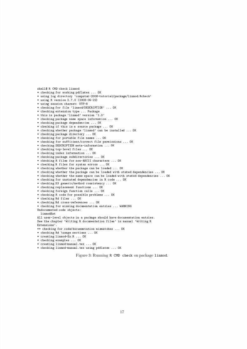
R CMD check helps you do quality assurance on packages:

• The directory structure and the format of DESCRIPTION are checked.

• The documentation is converted into text, HTML, and LATEX, and run through latex if available.

• The examples are run.

16



shell$ R CMD check linmod

* checking for working pdflatex ... OK

* using log directory ’compstat-2008-tutorial/package/linmod.Rcheck’

* using R version 2.7.0 (2008-04-22)

* using session charset: UTF-8

* checking for file ’linmod/DESCRIPTION’ ... OK

* checking extension type ... Package

* this is package ’linmod’ version ’1.0’

* checking package name space information ... OK

* checking package dependencies ... OK* checking if this is a source package ... OK

* checking whether package ’linmod’ can be installed ... OK

* checking package directory ... OK

* checking for portable file names ... OK

* checking for sufficient/correct file permissions ... OK

* checking DESCRIPTION meta-information ... OK

* checking top-level files ... OK

* checking index information ... OK

* checking package subdirectories ... OK

* checking R files for non-ASCII characters ... OK

* checking R files for syntax errors ... OK

* checking whether the package can be loaded ... OK

* checking whether the package can be loaded with stated dependencies ... OK

* checking whether the name space can be loaded with stated dependencies ... OK

* checking for unstated dependencies in R code ... OK

* checking S3 generic/method consistency ... OK* checking replacement functions ... OK

* checking foreign function calls ... OK

* checking R code for possible problems ... OK

* checking Rd files ... OK

* checking Rd cross-references ... OK

* checking for missing documentation entries ... WARNING

Undocumented code objects:

linmodEst

All user-level objects in a package should have documentation entries.

See the chapter ’Writing R documentation files’ in manual ’Writing R

Extensions’.

** checking for code/documentation mismatches ... OK

* checking Rd \usage sections ... OK

* creating linmod-Ex.R ... OK

* checking examples ... OK

* creating linmod-manual.tex ... OK* checking linmod-manual.tex using pdflatex ... OK

Figure 3: Running R CMD check on package linmod.

17



• Any tests in the tests/ subdirectory are run.

• Undocumented objects, and those whose usage and definition disagree are reported.

Figure 3 shows the output of R command check when run on package linmod. There is onewarning, because we have not documented function linmodEst.

R CMD build will create a compressed package file from your package directory. It does thisin a reasonably intelligent way, omitting object code, emacs backup files, and other junk. Theresulting file is easy to transport across systems and can be INSTALLed without decompressing. R

CMD build makes source packages by default. If you want to distribute a package that contains Cor Fortran for Windows users, they may well need a binary package, as compiling under Windowsrequires downloading exactly the right versions of quite a number of tools. Binary packages arecreated by

• INSTALLing the source package and then making a zip file of the installed version, or

• running R CMD build --binary.

For our package building a source package looks like

shell$ R CMD build linmod

* checking for file ’linmod/DESCRIPTION’ ... OK

* preparing ’linmod’:

* checking DESCRIPTION meta-information ... OK

* removing junk files

* checking for LF line-endings in source and make files

* checking for empty or unneeded directories

* building ’linmod_1.0.tar.gz’

and results in a file linmod_1.0.tar.gz which we can pass to other people.If you have a package that does something useful and is well-tested and documented, you might

want other people to use it, too. Contributed packages have been very important to the successof R (and before that of S). Packages can be submitted to CRAN by ftp. Make sure to run R CMD

check with the latest version of R before submission. The CRAN maintainers will make sure thatthe package passes CMD check (and will keep improving CMD check to find more things for youto fix in future versions). Submit only the package sources, binaries are built automatically bydesignated platform maintainers.

7 Summary

In this paper we have given step-by-step instructions on how to write code in R which conformsto standards for statistical models and hence is intuitive to use. Object oriented programmingallows the usage of common generic functions like summary() or predict() for a wide range of

different model classes. Using S formulas we can create design matrices with possibly complexinteraction and nesting structures. We then have turned a loose collection of functions into aregular R package, which can easily be documented, checked and distributed to other users. Thetutorial is meant as a starting point only. The R packaging system has much more features thanwe have covered, most of which are not necessary when first creating an R package.

Acknowledgements

R is a is the result of a collaborative effort and much of the software presented in this paper hasbeen implemented by other members of the R Development Core Team than the author of thisarticle. Parts of the text of this tutorial have been copied from the R documentation or othermaterial written by R Core.

18



References

BECKER, R. A., CHAMBERS, J. M. and WILKS, A. R. (1988): The New S Language .

Chapman & Hall, London, UK.CHAMBERS, J. M. (1998): Programming with data: A guide to the S language . SpringerVerlag, Berlin, Germany.

CHAMBERS, J. M. and HASTIE, T. J. (1992): Statistical Models in S . Chapman & Hall,London, UK.

GENTLE, J. E. (1998): Numerical Linear Algebra for Applications in Statistics . SpringerVerlag, New York, USA.

HORNIK, K. (2004): R: The next generation. In: J. Antoch (Ed.): Compstat 2004 — Proceed-ings in Computational Statistics . Physica Verlag, Heidelberg, 235–249. ISBN 3-7908-1554-3.

LEISCH, F. (2002): Sweave: Dynamic generation of statistical reports using literate data

analysis. In: W. Hardle and B. Ronz (Eds.): Compstat 2002 — Proceedings in Computational Statistics . Physica Verlag, Heidelberg, 575–580. ISBN 3-7908-1517-9.

LEISCH, F. (2003): Sweave, part II: Package vignettes. R News , 3(2), 21–24.

LIGGES, U. (2003): R help desk: Package management. R News , 3(3), 37–39 .

R Development Core Team (2008): R: A language and environment for statistical computing .R Foundation for Statistical Computing, Vienna, Austria. ISBN 3-900051-07-0.

R Development Core Team (2008a): R Installation and Administration . R Foundation forStatistical Computing, Vienna, Austria. ISBN 3-900051-09-7.

R Development Core Team (2008b): Writing R Extensions . R Foundation for Statistical

Computing, Vienna, Austria. ISBN 3-900051-11-9.

ROSSINI, A. J., HEIBERGER, R. M., SPARAPANI, R., MACHLER, M. and HORNIK, K.(2004): Emacs speaks statistics: A multiplatform, multipackage development environmentfor statistical analysis. Journal of Computational and Graphical Statistics , 13(1), 247–261.

TIERNEY, L. (2003): Name space management for R. R News , 3(1), 2–6 .

VENABLES, W. N. and RIPLEY, B. D. (2002): Modern Applied Statistics with S. Fourth Edition . Springer. ISBN 0-387-95457-0.

Documents

Creating R Packages - A Tutorial