CRB analysis of planar antenna arrays for optimizing near

Contents lists available at ScienceDirect

Signal Processing

Signal Processing 127 (2016) 117–134

http://d0165-16

E-mmarc.ca

journal homepage: www.elsevier.com/locate/sigpro

CRB analysis of planar antenna arrays for optimizing near-fieldsource localization

Jean Pierre Delmas a, Mohammed Nabil El Korso b, Houcem Gazzah c,Marc Castella a

a Telecom SudParis, CNRS UMR 5157, Université Paris Saclay, Evry, Franceb Université Paris Ouest Nanterre La Défense, LEME laboratory EA 4416, Francec Department of Electrical and Computer Engineering, University of Sharjah, 27272, UAE

a r t i c l e i n f o

Article history:Received 5 June 2015Received in revised form2 October 2015Accepted 24 February 2016Available online 7 March 2016

Keywords:Cramér Rao bound (CRB)Near-field source localizationAzimuthElevationRangePlanar antenna arraySensor's position optimization

x.doi.org/10.1016/j.sigpro.2016.02.02184/& 2016 Elsevier B.V. All rights reserved.

ail addresses: jean-pierre.delmas@[email protected] (M. Castella).

a b s t r a c t

This paper focuses on the Cramér Rao bound (CRB) of the azimuth, elevation and rangewith planar arrays for narrowband near-field source localization, using the exactexpression of the time delay. Specifically, the aim of this paper is twofold. First, we deriveexplicit non-matrix closed-form expressions of approximations of these three CRBs.Second, we use these expressions to optimize near-field source localization. For derivingthese expressions, we introduce conditions on the array geometry that allow us todecouple the azimuth, elevation and range parameters to a certain order in λ=r (in which λ

and r denote the wavelength and the range, respectively). A particular attention is given tothe popular array configurations which are the concentric uniform circular-based arrays,cross and square-based centro-symmetric arrays which satisfy these conditions. In orderto control directions of arrivals (DOA) ambiguity, we propose a new criterion, whichallows us to design non-uniform square [resp., cross]-based centro-symmetric arrayconfigurations with improved near-field range estimation capabilities without deterior-ating the DOA precisions w.r.t. uniform square [resp., cross]-based arrays. Finally, wespecify the accuracy of our proposed approximated CRBs'expressions and isotropy'sconditions w.r.t. the range and the number of sensors.

& 2016 Elsevier B.V. All rights reserved.

1. Introduction

Sensor placement is known to have a significant impact on the source localization capabilities of the antenna array, andthe topic starts to attract an increasing research effort [1–5]. Performance analysis based on the CRB is generally preferredbecause the latter is, at the same time, algorithm-independent and achievable by a number of popular algorithms.Dependence of the CRB on the array configuration has, first, been studied in relation to DOA estimation of far-field sources[6,7], assuming a planar wavefront is impinging on each sensor. The more challenging near-field case implies a curvature ofthe waves and a more complicated time delay model parameterized by the source DOA and range too. In the litterature, onecan find a plethora of near-field performance analysis based on an approximate propagation model applicable to the so-called Fresnel zone [8,9,10]. Only lately has the exact time delay formula been used for deriving more accurate closed-form

s.eu (J.P. Delmas), [email protected] (M.N. El Korso), [email protected] (H. Gazzah),

www.sciencedirect.com/science/journal/01651684

www.elsevier.com/locate/sigpro

http://dx.doi.org/10.1016/j.sigpro.2016.02.021



http://crossmark.crossref.org/dialog/?doi=10.1016/j.sigpro.2016.02.021&domain=pdf



mailto:[email protected]





J.P. Delmas et al. / Signal Processing 127 (2016) 117–134118

expressions of the CRB. This approach, applied to uniform linear arrays (ULA) [11], arbitrary linear arrays [12] and uniformcircular arrays (UCA) [13], is extended for the first time, here, to planar antenna arrays.

The aim of this paper is twofold: first, we tackle the problem of the derivation of explicit non-matrix closed-formexpressions of approximate CRB of the azimuth, elevation and range with for narrowband near-field source localization bymeans of planar arrays. Those derivations are based on the exact expression of the time delay parameter which is verychallenging due to the non-linearity of the exact propagation model. Concentrated on the azimuth, elevation and rangeparameters ðθ;ϕ; rÞ, the stochastic and deterministic CRBs, that are proportional (one to the other), are given by the inverseof a Fisher-like information matrix, whose terms are nonlinear expressions of θ, ϕ, r, and the coordinates of the sensors. Toobtain simple and interpretable expressions of the CRBs on θ, ϕ and r, we first specify conditions on the coordinates of thesensors that allow us to decouple θ, ϕ and r to a certain order in 1=r for near-field sources. Using Taylor expansions, weexplicit the expressions of the CRBs for three classes of planar arrays that satisfy these conditions: the concentric uniformcircular based-arrays, the square-based and cross-based centro-symmetric arrays. In particular, we study decoupling inrelationship with isotropy which is the array ability to exhibit the same accuracy in all azimuth look directions. In the far-field, estimation is decoupled if and only if it is isotropic. In contrast, we prove that, in the array near-field, the condition thatensures decoupling does not assure exact isotropy.

Second, we focus on the class of square and cross-based centro-symmetric arrays and highlight some of their attractivefeatures. In particular, we identify key geometric parameters that control the near-field array performance. Opportunisti-cally, these geometric parameters are used to design non-uniform square and cross-based centro-symmetric arrays thatachieve better near-field localization accuracy. More precisely, this design reduces (by as much as 60%) the CRB of the rangeparameter, with identical azumuth's and elevation's CRB as their corresponding uniform square and cross-based arrays.Finally, it should be noted that the proposed CRB-minimizing criterion incorporates some geometric constrains to accountfor the array ambiguity problem.

The paper is organized as follows. Section 2 specifies the data model, formulates the problem and gives the generalexpression of the CRB. In Section 3, we use Taylor expansions to derive the CRB for planar arrays. We focus on the followingthree classes which happen to exhibit decoupled estimation of the source parameters: the concentric uniform circularbased-arrays, the square-based and cross-based centro-symmetric arrays. An analysis of these CRBs is presented in Section 4while paying attention to isotropy and its dependency on the source range and the number of sensors. We also designoriginal non-uniform square and cross-based centro-symmetric arrays with improved near-field angle and range estimationcapabilities w.r.t. their uniform counter-parts. The paper is concluded in Section 5. Note that the part dedicated to the UCAwith a single circle has been partially presented in [13].

2. Data model and general expression of the CRB

2.1. Data model

A planar antenna array is made of P omni-directional sensors ðCpÞp ¼ 1;…;P placed in the ½O; x; yÞ plane, at coordinatesðxp; ypÞp ¼ 1;…;P . Without loss of generality, we assume the array centroid to be at the origin O of this plane. A source S locatedin the antenna array near-field has its position characterized by an azimuth angle θA ½0;2π�, an elevation angle ϕA ½0; π=2�and a range r (grouped in the vector α¼ ½θ;ϕ; r�T ), as illustrated in Fig. 1 for the concentric uniform circular based-arrays. Thesource is radiating a narrow-band signal, with wavelength λ, in the presence of an additive noise with complex envelope nk.The complex envelope xk of the signal collected by this array of sensors is modeled as

xk ¼ skaðαÞþnk; k¼ 1;…;K;

where sk is the source signal measured at the origin and aðαÞ ¼ ½eiτ1ðαÞ;…; eiτpðαÞ;…; eiτP ðαÞ�T is the so-called steering vector,where τpðαÞ is defined as τpðαÞ ¼ 2πðSO�SCpÞ=λ with SO¼r and ½SCp�2 ¼ ðxp�r sin ϕ cos θÞ2þðyp�r sin ϕ sin θÞ2þr2 cos 2ϕ (see Fig. 1 dedicated to the concentric uniform array) can be rewritten as

τp αð Þ ¼ 2πrλ

1�ffiffiffiffiffiβp

q� �ð1Þ

with

βp ¼def1�2 sin ϕxpr

cos θþypr

sin θ

� �þx2pþy2p

r2: ð2Þ

Based on K snapshots ðxkÞk ¼ 1;…;K , estimates of ðθ;ϕ; rÞ are obtained using a variety of algorithms, among which a few arecapable of achieving asymptotically the stochastic CRB [14] that we adopt as our performance measure of the array accuracy.

2.2. General expression of the CRB

Expressions of the CRB are available under the usual statistical properties about sk and nk: (i) sk and nk are independent,(ii) ðnkÞk ¼ 1;…;K are independent, zero-mean circular Gaussian distributed with covariance σ2nIP , (iii) ðskÞk ¼ 1;…;K are assumed

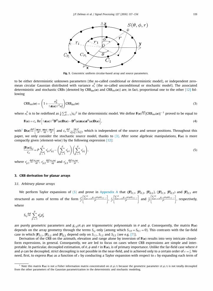
Fig. 1. Concentric uniform circular-based array and source parameters.

J.P. Delmas et al. / Signal Processing 127 (2016) 117–134 119

to be either deterministic unknown parameters (the so-called conditional or deterministic model), or independent zero-mean circular Gaussian distributed with variance σs

2(the so-called unconditional or stochastic model). The associated

deterministic and stochastic CRBs (denoted by CRBdetðαÞ and CRBstoðαÞ) are, in fact, proportional one to the other [12] fol-lowing

CRBsto αð Þ ¼ 1þ σ2nJaðαÞJ2σ2s

!CRBdet αð Þ ð3Þ

where σs2is to be redefined as 1

K

Pkk ¼ 1 skj2

�� in the deterministic model. We define FðαÞ ¼def ½CRBstoðαÞ��1 proved to be equal to

FðαÞ ¼ cσ Re JaðαÞJ2DHðαÞDðαÞ�DHðαÞaðαÞaHðαÞDðαÞh i

; ð4Þ

with1 D αð Þ ¼def ∂aðαÞ∂θ ; ∂aðαÞ∂ϕ ; ∂aðαÞ∂r

h iand cσ ¼def 2Kσ4s

σ2nðσ2n þPσ2s Þ, which is independent of the source and sensor positions. Throughout this

paper, we only consider the stochastic source model, thanks to (3). After some algebraic manipulations, FðαÞ is morecompactly given (element-wise) by the following expression [12]:

½FðαÞ�i;jcσ

¼ PXPp ¼ 1

τ0p;iτ0p;j�

XPp ¼ 1

τ0p;i

! XPp ¼ 1

τ0p;j

!; ð5Þ

where τ0p;1 ¼def ∂τpðαÞ

∂θ , τ0p;2 ¼def ∂τpðαÞ

∂ϕ and τ0p;3 ¼def ∂τpðαÞ

∂r .

3. CRB derivation for planar arrays

3.1. Arbitrary planar arrays

We perform Taylor expansions of (5) and prove in Appendix A that ð½F�1;1, ½F�1;2, ½F�2;2), (½F�1;3, ½F�2;3Þ and ½F�3;3 are

structured as sums of terms of the form r2

λ2

Pk

ℓ ¼ 0gℓ;kðθ;ϕÞSℓ;k� ℓ

rk

� , r

λ2

Pk


rk

� and 1

λ2

Pk


rk

� , respectively,

where

Si;j ¼defXPp ¼ 1

xipyjp

are purely geometric parameters and gℓ;kðθ;ϕÞ are trigonometric polynomials in θ and ϕ. Consequently, the matrix FðαÞdepends on the array geometry through the terms Si;j only (among which S1;0 ¼ S0;1 ¼ 0). This contrasts with the far-fieldcase in which ½F�1;1, ½F�1;2 and ½F�2;2 depend only on S1;1, S1;2 and S2;2 (see e.g. [7]).

Derivation of the CRB on the azimuth, elevation and range alone by inversion of FðαÞ results into very intricate closed-form expressions, in general. Consequently, we are led to focus on cases where CRB expressions are simple and inter-pretable. In particular, decoupled estimation, of θ, ϕ and r in FðαÞ, is of primary importance. Unlike the far-field case where θ

and ϕ can be decoupled, strict decoupling is not possible in the near-field, and is achieved only to a certain order of ϵ¼ λr. We

need, first, to express FðαÞ as a function of ϵ by conducting a Taylor expansion with respect to ϵ by expanding each term of

1 Note this matrix FðαÞ is not a Fisher information matrix concentrated on ðθ;ϕ; rÞ because the geometric parameter ðθ;ϕ; rÞ is not totally decoupledfrom the other parameters of the Gaussian parametrization in the deterministic and stochastic modeling.


FðαÞ as a weighted sum of unit-less terms

Sl;k� l

rk¼ Sl;k� l

λkλ

r

� �k

¼PP

p ¼ 1 xlpy

k� lp

λk

!ϵk;

in which ðxp; ypÞp ¼ 1;…;P and λ are fixed, but r can vary. For example, the unit-less term ½F�1;1 is structured asP2ℓ ¼ 0 gℓ;2ðθ;ϕÞSℓ;2�ℓ

λ2

!þ

P3ℓ ¼ 0 gℓ;3ðθ;ϕÞSℓ;3�ℓ

λ3

!ϵþ

P4ℓ ¼ 0 gℓ;4ðθ;ϕÞSℓ;4�ℓ

λ4

!ϵ2þo ϵ2

�;

where oðϵ2Þ gathers all the remaining term of ½F�1;1 with limϵ-0oðϵÞ=ϵ¼ 0. Focusing on the r dependence, ½F�1;1 is thusstructured as b1;10 þb1;11 ϵþb1;12 ϵ2þoðϵ2Þ. Applying this same expansion methodology to all the terms of FðαÞ ultimately, leadsto the expression

FðαÞ ¼b1;10 þb1;11 ϵþb1;12 ϵ2þoðϵ2Þ b1;20 þb1;21 ϵþb1;22 ϵ2þoðϵ2Þ b1;32 ϵ2þb1;33 ϵ3þoðϵ3Þb1;20 þb1;21 ϵþb1;22 ϵ2þoðϵ2Þ b2;20 þb2;21 ϵþb2;22 ϵ2þoðϵ2Þ b2;32 ϵ2þb2;33 ϵ3þoðϵ3Þ

b1;32 ϵ2þb1;33 ϵ3þoðϵ3Þ b2;32 ϵ2þb2;33 ϵ3þoðϵ3Þ ϵ4ðb3;34 þb3;35 ϵþb3;36 ϵ2þoðϵ2ÞÞ

2664

3775: ð6Þ

We first calculate off-diagonal terms in order to identify decoupling conditions. After tedious algebraic manipulations,they are found to be given by

cr2 sin ϕ cos ϕ

½F�1;2 ¼ PS0;2�S2;0

r2sin θ cos θþS1;1

r2cos 2θ

� �þo ϵ2 � ð7Þ

2cr sin ϕ

½F�1;3 ¼ PS0;3r3

cos θ 1� sin 2ϕ sin 2θ� �

�S3;0r3

sin θ 1� sin 2ϕ cos 2θ� ��

þS2;1r3

cos θ 1� sin 2ϕ cos 2θþ2 sin 2ϕ sin 2θ� �

�S1;2r3

sin θ 1� sin 2ϕ sin 2θþ2 sin 2ϕ cos 2θ� ��

þo ϵ3 �

ð8Þ

2cr cos ϕ

½F�2;3 ¼ PS0;3r3

sin θ 1� sin 2ϕ sin 2θ� �

þS3;0r3

cos θ 1� sin 2ϕ cos 2θ� ��

þS2;1r3

sin θ 1�3 sin 2ϕ cos 2θ� �

þS1;2r3

cos θ 1�3 sin 2ϕ sin 2θ� ��

þo ϵ3 �

; ð9Þ

where c¼def λ2

4π2cσ.

Second, we seek to decouple θ and ϕ to the zero order in ϵ (i.e., by imposing b1;20 ¼ 0) and to decouple ðθ;ϕÞ and r to thesecond order in ϵ (i.e., by imposing b1;32 ¼ b2;32 ¼ 0). Equalizing b1;20 to zero, i.e., the term S0;2 � S2;0

r2 sin θ cos θþS1;1r2 cos 2θ

� �of

(7) implies

S1;1 ¼ 0 and S2;0 ¼ S0;2; ð10Þwhich concurs with far-field conditions given in [7,16] for which θ and ϕ estimations are both decoupled and isotropic (w.r.t.the azimuth θ).

In the same way, both b1;32 of (8) and b2;32 of (9) are zero if S0;3 ¼ S1;2 ¼ S2;1 ¼ S3;0 ¼ 0. Careful examination of FðαÞ termsshows that these latter conditions also imply b1;11 ¼ b2;21 ¼ b1;21 ¼ 0. Ultimately, to ease the inversion of FðαÞ, we need b3;35 ¼ 0.The latter is satisfied under the additional conditions S0;5 ¼ S1;4 ¼ S2;3 ¼ S3;2 ¼ S4;1 ¼ 0. All these conditions are simulta-neously expressed by the following:

S1;1 ¼ 0; S0;2 ¼ S2;0 and Si;j ¼ 0 for iþ j¼ 3;5: ð11ÞWe note that these conditions (11) which include the far-field conditions (10) are much more severe. For example the V-shaped antenna array highlighted in [7] satisfies (10) but no longer satisfies (11).

Under the conditions (11), (6) simplifies to

FðαÞ ¼b1;10 þb1;12 ϵ2þoðϵ2Þ b1;22 ϵ2þoðϵ2Þ b1;33 ϵ3þoðϵ3Þ

b1;22 ϵ2þoðϵ2Þ b2;20 þb2;22 ϵ2þoðϵ2Þ b2;33 ϵ3þoðϵ3Þb1;33 ϵ3þoðϵ3Þ b2;33 ϵ3þoðϵ3Þ ϵ4ðb3;34 þb3;36 ϵ2þoðϵ2ÞÞ

2664

3775 ð12Þ

making it possible to obtain, after straightforward algebraic manipulations, the following expressions of the CRBs:

CRB θð Þ ¼ 1

b1;10

1�ϵ2b1;12

b1;10

� ðb1;33 Þ2b1;10 b3;34

! !þo ϵ2 � ð13Þ

CRB ϕð Þ ¼ 1

b2;20

1�ϵ2b2;22

b2;20

� ðb2;33 Þ2b2;20 b3;34

! !þo ϵ2 � ð14Þ


CRB rð Þ ¼ 1

b3;34 ϵ41�ϵ2

b3;36

b3;34

� ðb1;33 Þ2b1;10 b3;34

� ðb2;33 Þ2b2;20 b3;34

!þo ϵ2 � !

: ð15Þ

The fact that

limr-1

CRB θð Þ ¼ CRBFF θð Þ ¼ 1

b1;10

and limr-1

CRB ϕð Þ ¼ CRBFF ϕð Þ ¼ 1

b2;20

; ð16Þ

where CRBFFðθÞ and CRBFFðϕÞ denote the far-field CRBs, means that arrays satisfying conditions (11) do achieve the far-fieldCRBs when the source-to-array distance r tends to infinity. In contrast, arrays that do not satisfy conditions (11) do notnecessary satisfy (16) (see an example for linear arrays in [12]), an unexpected behavior due to a possible coupling (b1;32 a0,b2;32 a0) between ðθ;ϕÞ and r in FðαÞ to the second-order in ϵ. Finally, for a source in the plane (x,y), (15) reduces to

CRB rð Þ ¼ 1

b3;34 ϵ41�ϵ2

b3;36

b3;34

� ðb1;33 Þ2b1;10 b3;34

!þo ϵ2 � !

ϕ ¼ π=2

: ð17Þ

3.2. Special classes of arrays: expressions of FðαÞ

Conditions (11) are satisfied by many structured planar arrays. We study in details the following three classes of planararrays for which the expression of FðαÞ are derived, as well as expressions (13)–(15) of the CRBs.

3.2.1. Concentric uniform circular-based arraysThe P sensors are divided into I groups of respective sizes P1;…; PI where

PIi ¼ 1 Pi ¼ P. The i-th group of sensors is placed

uniformly along a circle of radius ri so that sensor pi, pi ¼ 1;…; Pi forms an angle θpi ;i ¼def

θiþθ�2πðpi �1ÞPi

with ½O; xÞ, θi being anarbitrarily selected offset angle.2 Parameter βp of the phase τp given in (1) can be expressed as

βp ¼ 1�2rir

cos θpi ;i sin ϕþr2ir2

ð18Þ

associated with a sensor on a circle of radius ri. Using the identity

XPi

pi ¼ 1

eikθpi ;i ¼ Pieikθ if k=PiAN

0 k otherwise

(; ð19Þ

we easily prove that conditions (11) are satisfied if each circle include more than 5 (Pi45, for all i) sensors.By using the sensors polar coordinates ðri; θpi ;iÞ, the following Taylor expansions of the terms of the matrix FðαÞ are proved

in Appendix B.1 for PiZ6:

2c

r2 sin 2ϕ½F�1;1 ¼ P

XIi ¼ 1

Pir2ir2�r4ir4

cos 2ϕ

� �þo ϵ4 � ð20Þ

2cr2 cos 2ϕ

½F�2;2 ¼ PXIi ¼ 1

Pir2ir2�r4ir4

1�3 sin 2ϕ� ��

�XIi ¼ 1

P2i

2r4ir4

sin 2ϕ�Xia j

PiPjr2i r

2j

r4sin 2ϕþo ϵ4

� ð21Þ

c

r2 sin 3ϕ cos ϕ½F�1;2 ¼ o ϵ4

� ð22Þ

c

r sin 4ϕ½F�1;3 ¼ o ϵ4

� ð23Þ

cr cos ϕ

½F�2;3 ¼ PXIi ¼ 1

Pi

4r4ir4

3�94sin 2ϕ

� �sin ϕ�

XIi ¼ 1

P2i

4r4ir4

1þ12sin 2ϕ

� �sin ϕ�1

4

Xia j

Pj

r2i r2j

r4Pj�

Pi

2sin 2ϕ

� �þo ϵ4 � ð24Þ

c½F�3;3 ¼ PXIi ¼ 1

Pir4ir4g1 sin 2ϕ� �

�XIi ¼ 1

P2ir4ir4g2 sin 2ϕ� �

þPXIi ¼ 1

Pir6ir6g3 sin 2ϕ� �

�XIi ¼ 1

P2ir6ir6g4 sin 2ϕ� �

�Xia j

PiPjr2i r

4j

r6g4 sin 2ϕ� �

þo ϵ4 �

; ð25Þ

where ϵ¼defmaxiðriÞr . Exact expressions of polynomials g1, g2, g3 and g4 are given in Appendix B.1.1.

2 These arrays are centro-symmetric, only if ðPiÞi ¼ 1,.., I are all even. They include as particular case, the so-called uniform concentric circular arrays [15]where θi ¼ 0 and the number Pi of sensors on each circle Ci is constant.


3.2.2. Cross-based and square-based centro-symmetric arraysFor cross-based centro-symmetric arrays, as shown in Fig. 2, sensors are placed along the x-axis and the y-axis, sym-

metrically around the origin, i.e., at coordinates ð7aq;0Þ and ð0; 7aqÞ, resulting in a total number of sensors P ¼ 2Q�1 orP ¼ 2Q depending on whether a sensor is placed at the origin or not, where Q is the number of sensors on each axis. Wehave Si;j ¼ 0 for arbitrary ia0 and ja0, hence satisfying conditions (11). Non-zero geometric parameters Si;j arePQ

q ¼ 1 a2q ¼ S2;0 ¼ S0;2 ¼defΣ2,

PQq ¼ 1 a

4q ¼ S4;0 ¼ S0;4 ¼defΣ4 and

PQq ¼ 1 a

6q ¼ S6;0 ¼ S0;6 ¼defΣ6.

Square-based centro-symmetric arrays shown in Fig. 3 are made of P ¼Q2 sensors at positions ðaq; aq0 Þq ¼ 1;…;Q ;q0 ¼ 1;…;Q

such that if a sensor is placed at some position ðxp; ypÞ, another one is placed in the coordinate ð�xp; �ypÞ. Si;j are found to

satisfy conditions (11). Non-zero ones reduce to S2;0 ¼ S0;2 ¼defQΣ2, S4;0 ¼ S0;4 ¼defQΣ4, S6;0 ¼ S0;6 ¼defQΣ6, S2;2 ¼ Σ22, and

S4;2 ¼ S2;4 ¼ Σ2Σ4, where Σ2, Σ4 and Σ6 have the same definition as for the cross-based arrays.For these two (cross and square based) classes of centro-symmetric arrays, we reach the following unified expression3 of

the Taylor expansion of the matrix FðαÞ, proved in Appendix C:

c

r2 sin 2ϕ½F�1;1 ¼

a1;12 Σ2

r2þa1;14 ðθ;ϕÞQΣ4þa1;1

22 ðθ;ϕÞΣ22

r4þo ϵ4 � ð26Þ

cr2 cos 2ϕ

½F�2;2 ¼a2;22 Σ2


22 ðθ;ϕÞΣ22


c

r2 sin 3ϕ cos ϕ½F�1;2 ¼

a1;24 ðθ;ϕÞQΣ4þa1;222

ðθ;ϕÞΣ22


c

r sin 4ϕ½F�1;3 ¼

a1;34 ðθ;ϕÞQΣ4þa1;322 ðθ;ϕÞΣ2

2


cr sin ϕ cos ϕ

½F�2;3 ¼a2;34 ðθ;ϕÞQΣ4þa2;3

22ðθ;ϕÞΣ2

2


c½F�3;3 ¼a3;34 ðθ;ϕÞQΣ4þa3;3

22 ðθ;ϕÞΣ22

r4þa3;36 ðθ;ϕÞQ2Σ6þa3;32;4ðθ;ϕÞQΣ2Σ4þa3;3

23 ðθ;ϕÞΣ32

r6þo ϵ6 �

; ð31Þ

where a1;12 ¼ a2;22 ¼ P [resp., PQ] for the cross-based [resp., square-based] centro-symmetric arrays. Expressions of ai;jk ðθ;ϕÞ,given in Appendix C, are functions of the number of sensors and ðθ;ϕÞ. Also, a1;1

22ðθ;ϕÞ ¼ a1;2

22ðθ;ϕÞ ¼ a1;3

22 ðθ;ϕÞ ¼ a3;323 ðθ;ϕÞ ¼ 0 for

the cross-based centro-symmetric arrays.

3.3. Special classes of arrays: Expressions of the CRBs

3.3.1. Concentric uniform circular-based arraysUsing (13) and the values of the parameters bi;jk of the matrix FðαÞ of (12) derived by identification with the expansion

(20)–(25), we deduce the following closed-form expression of the CRB on the azimuth:

CRBðθÞ ¼ CRBFF θð Þ 1þPI

i ¼ 1 Pir4i cos 2ϕ

r2PI

i ¼ 1 Pir2iþo ϵ2 � !

; ð32Þ

where we obtain the following original expression of the CRB on the azimuth under the far-field conditions:

CRBFF θð Þ ¼ 2c

sin 2ϕ

1

PPI

i ¼ 1 Pir2i: ð33Þ

For a single-ring UCA of radius r1, Eq. (32) simplifies to

CRB θð Þ ¼ CRBFF θð Þ 1þr21r2

cos 2ϕþor21r2

� �� ð34Þ

with CRBFF θð Þ ¼ 2csin 2ϕ

1P2r21

.Expressions of the CRB on the elevation and range deduced from (14) and (15) are much more intricate. Consequently, we

concentrate on the single-ring UCA for which we obtain the following closed-form expressions:

CRB ϕð Þ ¼ CRBFF ϕð Þ 1þr21r2h2 sin 2ϕ� �

þor21r2

� �� ð35Þ

3 Note that the number Q introduced in some terms will allow us to obtain the common expressions of the CRB (42), (43) and (44).

y

x

Fig. 3. Square-based centro-symmetric array.

x

y

Fig. 2. Cross-based centro-symmetric array.


CRB rð Þ ¼ 32c

sin 4ϕ

r4

r411þr21

r2h3 sin 2ϕ� �

þor21r2

� �� ; ð36Þ

with CRBFF ϕð Þ ¼ 2ccos 2ϕ

1P2r21

and

h2 sin 2ϕ� �

¼def 16

sin 2ϕþ39

4sin 2ϕ�27 and h3 sin 2ϕ

� �¼def5�21

4sin 2ϕ:

Further simplification are obtained for a single-ring UCA made of P48 sensors, for which (20), (22) and (23) become:

2c

r2 sin 2ϕ½F�1;1 ¼ P2 r21

r2�r41r4

cos 2ϕþr41r4g5 sin 2ϕ� �

þr61r6g6 sin 2ϕ� ��

þor71r7

� �ð37Þ

cr2 sin ϕ cos ϕ

½F�1;2 ¼ or71r7

� �ð38Þ

cr sin ϕ

½F�1;3 ¼ or71r7

� �; ð39Þ

with

g5ð sin 2ϕÞ ¼def1�3 sin 2ϕþ2 sin 4ϕ and g6ð sin 2ϕÞ ¼def �1þ6 sin 2ϕ�10 sin 4ϕþ5 sin 6ϕ:

This allows us to further develop the Taylor expansion in (34) to obtain the following more accurate closed-form expression:

CRB θð Þ ¼ CRBFF θð Þ 1þr21r2

cos 2ϕþr41r4

sin 2ϕ cos 2ϕþr61r6h1 sin 2ϕ� �

þor71r7

� �� ; ð40Þ

with h1ð sin 2ϕÞ ¼def � sin 2ϕþ3 sin 4ϕ�2 sin 6ϕ. Interestingly, for a source in the (x,y) plane (i.e., ϕ¼ π=2), we deduce from thematrix FðαÞ that (40) and (17) give

CRB θð Þ ¼ CRBFF θð Þ 1þor71r7

� ��

CRB rð Þ ¼ 32c

sin 4ϕ

r4

r411� r21

2r2þo

r21r2

� �� :

The validity of some approximate closed-form expressions of the CRB is illustrated for a source located with an azimuth θ¼ 701and elevation ϕ¼ 701. Figs. 4 and 5 compare the approximate ratios CRBðθÞ=CRBFFðθÞ and CRBðϕÞ=CRBFFðϕÞ given by (40) and (35)to the exact ones (i.e., derived from the numerical inversion of the matrix FðαÞ built on the exact model of the time delay 1). These


figures naturally show that CRB(θ) and CRB(ϕ) tend to CRBFFðθÞ and CRBFFðϕÞ, respectively, when the range increases. In addition, wecan notice that the far-field state is reached from the ratio r=r1 ¼ 10. We also see that the near-field CRB on the azimuth andelevation are smaller than the associated far-field CRB. We also consider Fig. 6 that compares the approximate CRBðrÞ (36) to theexact one as a function of r=r1. Figs. 4 and 6 show that the approximate values of CRB on the azimuth and range are very close to theexact ones for 10 sensors from r=r1 ¼ 2. This contrasts with elevation for which the approximate values of the CRB are close to theexact one only from r=r1 ¼ 4. For 7 sensors, we note that our proposed approximations of all CRBs are still accurate from r=r1 ¼ 4.

3.3.2. Cross-based and square-based centro-symmetric arraysFor such arrays, (13)–(15) give very intricate expressions. But hopefully, we can identify two geometric parameters κ and

η that determine the near-field accuracy of the antenna array. They are defined by the following two unit-less array geo-metric expressions:

κ¼def Σ22

QΣ4and η¼def Σ3

2

Q2Σ6: ð41Þ

We note that they verify 0oηrκr1 [12], and remain unchanged if a sensor is added/removed at/from the origin and ifsensor coordinates are scaled by some arbitrary constant. The interest of these two parameters is that they complement thegeometric parameter Σ2 to characterize the behavior of the three CRBs in the near-field condition, allowing us to derivesome optimizations. This contrasts with the far-field conditions for which Σ2 characterizes the behavior of the CRB on theazimuth and elevation in the near-field condition (see (41)).

After tedious algebraic manipulations, CRBs (13)–(15) can be rewritten in terms of these parameters, to obtain the fol-lowing expressions:

CRB θð Þ ¼ CRBFF θð Þ 1þaðθ;ϕ; κÞΣ2

r2þo ϵ2 ��

ð42Þ

CRB ϕð Þ ¼ CRBFF ϕð Þ 1þbðθ;ϕ; κÞΣ2

r2þo ϵ2 ��

ð43Þ

CRB rð Þ ¼ r4

dðθ;ϕ; κÞΣ22

1þeðθ;ϕ; κ; ηÞΣ2

r2þo ϵ2 ��

; ð44Þ

where the far-field CRB on θ and ϕ are given, respectively, by

CRBFF θð Þ ¼ c

a1;12 Σ2 sin 2ϕand CRBFF ϕð Þ ¼ c

a2;22 Σ2 cos 2ϕ; ð45Þ

in which a1;12 ¼ a2;22 ¼ P [resp., PQ] for the cross-based centro-symmetric arrays [resp., square-based centro-symmetricarrays] and

a θ;ϕ; κð Þ ¼a1;34 ðθ;ϕÞþκa1;3

22 ðθ;ϕÞ� �2

sin 6ϕ� a1;14 ðθ;ϕÞþκa1;122 ðθ;ϕÞ

� �a3;34 ðθ;ϕÞþκa3;3

22 ðθ;ϕÞ� �

κa1;12 a3;34 ðθ;ϕÞþκa3;322 ðθ;ϕÞ

� �

b θ;ϕ; κð Þ ¼a2;34 ðθ;ϕÞþκa2;3

22ðθ;ϕÞ

� �2sin 2ϕ� a2;24 ðθ;ϕÞþκa2;2

22ðθ;ϕÞ

� �a3;34 ðθ;ϕÞþκa3;3

22ðθ;ϕÞ

� �κa2;22 a3;34 ðθ;ϕÞþκa3;3

22ðθ;ϕÞ

� �d θ;ϕ; κð Þ ¼ 1

c1κa3;34 θ;ϕð Þþa3;3

22θ;ϕð Þ

� �

e θ;ϕ; κ; νð Þ ¼a1;34 ðθ;ϕÞþκa1;3

22ðθ;ϕÞ

� �2sin 6ϕ

κa1;12 a3;34 ðθ;ϕÞþκa3;322

ðθ;ϕÞ� �

þa2;34 ðθ;ϕÞþκa2;3

22 ðθ;ϕÞ� �2

sin 2ϕ

κa2;22 a3;34 ðθ;ϕÞþκa3;322

ðθ;ϕÞ� � �

η�1a3;36 ðθ;ϕÞþκ�1a3;32;4ðθ;ϕÞþa3;323 ðθ;ϕÞ

κ�1a3;34 ðθ;ϕÞþa3;322

ðθ;ϕÞ; ð46Þ

where the terms ai;jk ðθ;ϕÞ come from (26)–(31).The validity of some approximate closed-form expressions of the CRB for the square-based centro-symmetric arrays4 is

illustrated for a source located with an azimuth θ¼ 601 and elevation ϕ¼ 401 for the specific case of uniform square-basedarrays with half-wavelength inter-sensors spacing. As in the UCA case, Figs. 7 and 8 compare the approximate ratiosCRBðθÞ=CRBFFðθÞ and CRBðϕÞ=CRBFFðϕÞ given by (42) and (43) to the exact ones. Fig. 9 compares the approximate CRBðrÞ, given

4 The same behavior is noticed for the cross-based centro-symmetric arrays.

2 3 4 5 6 7 8 9 101

1.005

1.01

1.015

1.02

1.025

1.03

1.035

1.04

1.045

1.05

r/r1

P=7. Exact CRBP=7. Approx. CRBP=10. Exact CRBP=10. Approx. CRB

Fig. 4. Approximate and exact ratios CRBðθÞ=CRBFFðθÞ for the UCA.

2 3 4 5 6 7 8 9 100.9

0.95

1

1.05

1.1

1.15

r/r1

P=7. Exact CRBP=7. Approx. CRBP=10. Exact CRBP=10. Approx. CRB

Fig. 5. Approximate and exact ratios CRBðϕÞ=CRBFFðϕÞ for the UCA.

2 3 4 5 6 7 8 9 100.8

0.85

0.9

0.95

1

1.05

r/r1

P=7P=10

Fig. 6. Ratio of the approximate CRBðrÞ to the exact one for the UCA.


by (44), to the exact one as a function of r=r0 where r0 is the half aperture Q �12

λ2 (similarly as r=r1 for the UCA). The above

figures confirm the validity of the proposed approximations for a large enough Q and/or a large enough ratio r=r0.

2 4 6 8 10 12 14 16 18 200.9

1

1.1

1.2

1.3

1.4

1.5

1.6

r/r0

Q=4 Exact CRB

Q=2 Exact CRBQ=2 Approx. CRB

Q=4 Approx. CRB

Fig. 7. Approximate and exact ratios CRBðθÞ=CRBFFðθÞ for uniform square-based arrays.

2 4 6 8 10 12 14 16 18 20

0.5

1

1.5

2

2.5Q=2 Exact CRB

Q=4 Approx. CRBQ=4 Exact CRB

r/r0

Q=2 Approx. CRB

Fig. 8. Approximate and exact ratios CRBðϕÞ=CRBFFðϕÞ for uniform square-based arrays.

10 15 20 25 300.2

0.4

0.6

0.8

1

1.2

r/r

CR

B app

rox(.)

/CR

B tr

ue(.)

Q=6Q=4

Fig. 9. Ratio of the approximate CRBðrÞ to the exact one for uniform square-based arrays.



4. Analysis of the derived CRBs

4.1. Isotropy under the near-field

An antenna array appears to be isotropic to a source located in its far-field when sensors placed such that

S1;1 ¼ 0 and S0;2 ¼ S2;0:

This condition is weaker than conditions (11). Consequently, the isotropy property deteriorates if the source tends to be inthe antenna near-field. For example, for cross-based and square-based centro-symmetric arrays, the CRBs on azimuth (42)and elevation (43) depend on the azimuth angle to the second-order in ϵ, whereas for the CRB on the range (44), thedominant term is dependent on the azimuth. Furthermore, from expressions of ai;jk ðθ;ϕÞ in Appendix C, azimuth, elevationand range CRBs appear to be periodic in θ of period π=2, as one may expect. Due to the intricate expressions of these CRBs, itis difficult to learn more about the deterioration of isotropy when the source range r decreases or when the number ofsensors P decreases.

However, more can be learnt about single-ring UCA. First, thanks to (19), CRBs are periodic in θ of period 2π=P, as onemay predict. Also if we denote the radius by r1 and θp;1 by θp, Taylor expansion of the elements of FðαÞ w.r.t. ϵ (5), where onlythe θ dependence is retained, yields to

½F�i;j ¼X1k ¼ 0

XPp ¼ 1

gði;jÞk ð cos θp; sin θpÞ !

ϵk; ð47Þ

where gði;jÞk is a polynomial expression of cos θp and sin θp of degree kþ2, kþ1 or k for ði; j¼ 1;2Þ, ði¼ 1;2; j¼ 3Þ orði¼ j¼ 3Þ, respectively. By linearizing this polynomial, we have for example for i,j¼1,2:

gð1;2Þk ð cos θp; sin θpÞ ¼Xkþ2

ℓ ¼ 0

cð1;2Þℓ;k cos ðℓθpÞþXkþ2

ℓ ¼ 1

sð1;2Þℓ;k sin ðℓθpÞ

where cð1;2Þ0;k ¼ 0 for odd degrees of gð1;2Þk . Then, using (19), focusing on θ and carefully studying the first terms of the Taylorexpansion (47) in ϵ, we obtain

½F�i;j ¼XðP�3Þ=2b c

k ¼ 0

bi;j2kϵ2kþ

X1k ¼ P�2

bi;jk ðθÞϵk ð48Þ

½F�i;j ¼X1

k ¼ P�2


½F�2;3 ¼XP�1

k ¼ 3

bi;jk ϵkþ

X1k ¼ P


½F�3;3 ¼XðP�1Þ=2b c

k ¼ 2

bi;j2kϵ2kþ

X1k ¼ P

bi;jk ðθÞϵk; ð51Þ

for PZ4 and i¼ j¼ 1 or i¼ j¼ 2 (48), i¼ 1; j¼ 2;3 (49), where bi;jk and bi;j2k do not depend on θ. For example, 2c½F�1;1r20 sin

2ϕis given in

Table 1 for P ¼ 3;4;5;6.The following can be concluded about a single ring UCA of a fixed number P of sensors: From (48)–(51), matrix FðαÞ does

not depend on the azimuth up to the order P�3 in r1=r, and, from (49), θ and ðϕ; rÞ are decoupled up to the order P�1 inr1=r. Consequently, the azimuth's CRB does not depend on the azimuth up to the order P�1 in r1=r, in contrast to theelevation's and range's CRB for which this order is smaller or equal to P�3. Consequently, for fixed r (resp. P), isotropyincreases when P (resp. r) increases. Also, azimuth's CRB is much less sensitive to the azimuth angle than elevation andrange CRBs.

We introduce the following non-isotropy measurement, in which CRBðθÞ denotes the mean of CRBðθÞ w.r.t. θ,

ρ¼ supθ

jCRBðθÞ�CRBðθÞjCRBðθÞ

illustrated in Figs. 10 and 11 for single-ring UCAs and uniform square based arrays with half-wavelength inter-sensorsspacing, respectively. Fig. 10 shows that the isotropy is much more sensitive to P than to r, which increases very rapidly withr and P in contrast to Fig. 11 where the isotropy is less sensitive to Q and increases much less rapidly with r and Q. In otherwords, the UCAs are much more isotropic than the uniform square-based arrays for given half aperture and range, under thenear-field conditions.

Table 1

Second-order expansion of 2c½F�1;1r20 sin 2ϕ

for P ¼ 3;4;5;6.

P

3 1�ϵ2 sin ϕ cos 3θþoðϵ2Þ4 1�ϵ2ð cos 2ϕ� sin 2ϕ sin 4θÞþoðϵ2Þ5 1�ϵ2 cos 2ϕ�ϵ3 sin 3ϕ cos 5θþoðϵ3Þ6 1�ϵ2 cos 2ϕ�ϵ4ð1�3 sin 2ϕþ2 sin 4ϕ� sin 4ϕ cos 6θÞþoðϵ4Þ

2 3 4 5 6 7 8 9 1010

10

10

10

10

10

r/r

P=4P=6P=8P=10

Fig. 10. Non-isotropy criterion ρ w.r.t. r=r1 and P for UCAs.

2 3 4 5 6 7 8 9 1010

10

10

10

r/r0

ρ

Q=2Q=3Q=4Q=6

Fig. 11. Non-isotropy criterion ρ w.r.t. r=r0 and Q for uniform square-based arrays.


4.2. Optimization of cross-based and square-based centro-symmetric arrays

4.2.1. Optimization criterionFar-field (azimuth and elevation) performance is fully determined by the geometric parameter Σ2 and the number P of

sensors as expressed in (45), while near-field performance depends on geometric parameters κ and η for DOA and rangeestimation. In particular,the most significant term of the range CRB, as expressed in (44) and (46), is controlled by κ throughthe term5

r4

dðθ;ϕ; κÞΣ22

¼ cr4

Σ22

1κa3;34 θ;ϕð Þþa3;3

22θ;ϕð Þ

� �1

;

which is an increasing function of κ as a3;34 ðθ;ϕÞ40 for arbitrary θ and ϕ.

5 Here a3;34 ðθ;ϕÞ and a3;322 ðθ;ϕÞ are defined in (31).

0.3 0.35 0.4 0.45 0.5 0.55 0.6 0.650.2

0.4

0.6

0.8

1

1.2

1.4

1.6

1.8

κ

RQ

(κ)

P=36P=25P=16USA P=36USA P=25USA P=16

Fig. 12. RP ðκÞ as a function of κ for different square-based centro-symmetric arrays for θ¼ 601 and ϕ¼ 301.

0.3 0.35 0.4 0.45 0.5 0.55 0.6 0.65 0.70.2

0.4

0.6

0.8

1

1.2

1.4

1.6

1.8

κ

(θ0,φ

0)=(60°,30°)

(θ0,φ

1)=(60°,60°)

(θ0,φ

2)=(60°,75°)

(θ1,φ

0)=(30°,30°)

(θ2,φ

0)=(75°,30°)

Fig. 13. RPðκnuÞ as a function of κnu for square-based centro-symmetric arrays with P¼36 for different ðθ;ϕÞ.


Our array geometry optimization approach is inspired by the following rationale. For those arrays with predeterminedvalues of Σ2 and P (and so, ones with similar far-field performance), near-field range estimation depends mainly on Σ2 and κ.For comparison purposes, we refer to uniform cross (UCrA) and square-based (USA) arrays, for which κ is denoted κu. Weseek array geometries of nonuniform cross and square-based arrays, for which the κ-dependent criterion below is lowerthan one6:

RP κð Þ ¼ limr-1

CRBðrÞjnuCRBðrÞju

¼1κua3;34 θ;ϕð Þþa3;3

22 θ;ϕð Þ1κa

3;34 θ;ϕð Þþa3;3

22 θ;ϕð Þ: ð52Þ

While spanning 2Q;1h i

, extreme values of κ are to be avoided in order to preserve the DOA non-ambiguity of the cross-

based and square-based centro-symmetric arrays. More specifically, on the one hand, κ� 2Q corresponds to co-located

sensors at the centroid O, (except 4 sensors at ðxp; ypÞ ¼ ð7a;0Þ; ð0; 7aÞ for cross-based centro-symmetric arrays [resp.,ðxp; ypÞ ¼ ð7a; 7aÞ for square-based centro-symmetric arrays]). On the other hand, κ� 1 corresponds to aq � 7a (allsensors concentrated to the previous four positions). Consequently, we only seek values of κ in [0.3–0.7].

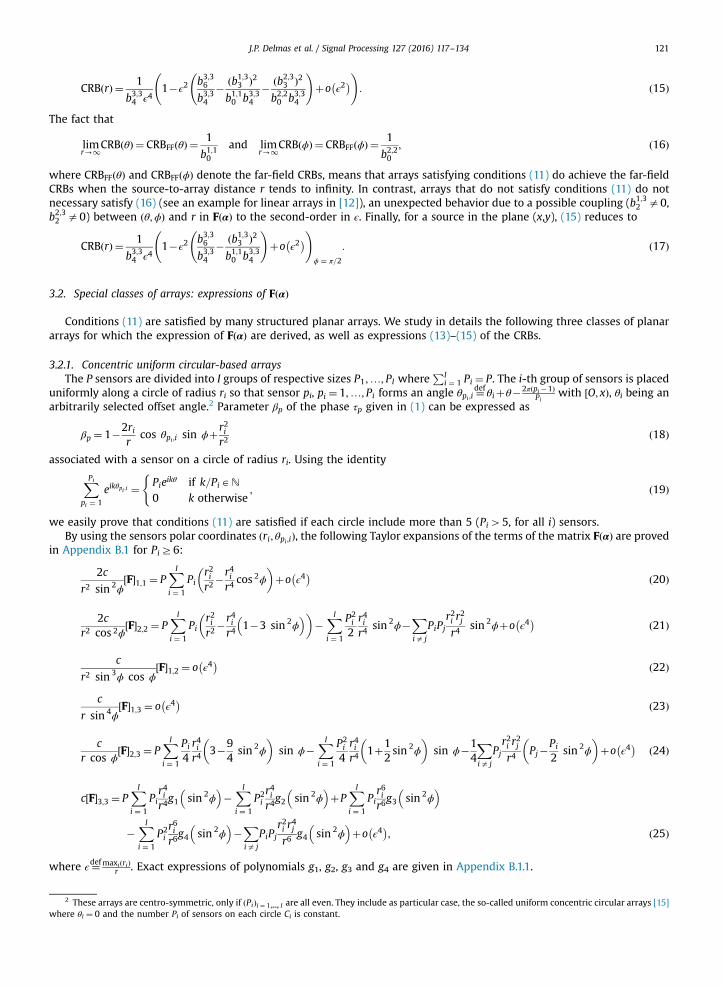
The ratio (52) illustrated in Fig. 12 shows that there exist non-uniform square or cross-based centro-symmetric arrayswith RPðκÞ significantly lower than 1, suggesting that there is an opportunity to achieve a great deal of improvement. This is,actually true regardless of the source DOA as confirmed by Fig. 13. This figure shows that RPðκÞ depends very loosely on θ

and ϕ. More precisely, it is not sensitive to θ due to the isotropy property, but little sensitive to ϕ. Furthermore the per-formance advantage increases for weak values of ϕ. The same behavior has been observed for cross-based centro-symmetricarrays.

6 Here CRBðrÞju and CRBðrÞjnu denote the CRB on r for, respectively, uniform and nonuniform cross and square-based arrays.

Table 3Values of κ, RPðκÞ, sensor positions, rCrCSPSL and rSCSPSL for Q¼7.

κ RPðκÞ Sensor positions rCrCSPSL rSCSPSLCriterion

0.5714 1 0; 70:1890; 70:3780; 70:5669 3.3400 16.6945 (54)0.5000 0.7571 0; 70:1674; 70:3348; 70:5999 2.6274 10.7527 (54)0.4500 0.6228 0; 70:1500; 70:3001; 70:6225 2.3674 6.7340 (54)0.4000 0.5098 0; 70:1288; 70:2577; 70:6458 2.5001 4.6751 (54)0.4000 0.5098 0; 70:1876; 70:2150; 70:6469 2.7278 (53)0.4000 0.5098 0; 70:1036; 70:2705; 70:6450 8.1699 (53)0.3500 0.4133 0; 70:1001; 70:2003; 70:6707 1.7784 3.4868 (54)0.3500 0.4133 0; 70:1278; 70:1828; 70:6709 1.8255 (53)0.3500 0.4133 0; 70:1376; 70:1753; 70:6710 3.7298 (53)

Table 2Values of κ, RP ðκÞ, sensor positions, rCrCSPSL and rSCSPSL for Q¼6.

κ RP ðκÞ Sensor positions rCrCSPSL rSCSPSLCriterion

0.5776 1 70:1195; 70:3586; 70:5976 2.9087 17.3310 (54)0.5000 0.7392 70:1012; 70:3036; 70:6305 2.8441 6.6667 (54)0.4500 0.6080 70:0866; 70:2599; 70:6519 2.3719 4.1762 (54)0.4000 0.4978 70:0674; 70:2022; 70:6742 1.7310 3.7037 (54)0.4000 0.4978 70:1335; 70:1640; 70:6748 1.8115 (53)0.4000 0.4978 70:0823; 70:1961; 70:6744 3.8124 (53)0.3500 0.4036 70:0349; 70:1047; 70:6984 1.1689 1.3889 (54)0.3500 0.4036 70:0332; 70:1052; 70:6984 1.1698 (53)0.3500 0.4036 70:0701; 70:0849; 70:6984 1.3952 (53)


4.2.2. Sensors placement

Having fixed Σ2, P and κA 2Q; κu� �

, based on desired near-field and far-field performance, there are ðQ=2Þ�2 for Q even,

[resp., ððQ�1Þ=2Þ�2 for Q odd] degrees of freedom for arbitrary cross or square-based centro-symmetric arrays to setpositions a1;…aQ of the sensors.7 They are used to tackle the array ambiguity problem, a crucial one for the nonuniformarray configurations.

Ambiguities occur when two steering vectors happen to be (very) close, despite referring to well-separated lookdirections [17]. One way to minimize ambiguities is to minimize the so-called relative peak sidelobe level (PSL) ratio [5]derived from the conventional array beampattern [18]; if

½aFFðθ;ϕÞ�p ¼def limr-1½aðαÞ�p ¼ e

i2πλ sin ϕ xp cos θþyp sin θð Þð Þ;

then

rPSL ¼def maxðu;vÞ outside the mainlobe region

jaHFFðu; vÞaFFðθ;ϕÞj2=P2:

Since

mina1 ;…aQ

rPSL ; ð53Þ

under the constraintsPQ

q ¼ 1 a2q ¼ Σ2,

PQq ¼ 1 a

4q ¼ Σ4 [with Σ4 ¼ Σ2

2=Qκ from (41)] and symmetric aq is a nonconvex mini-mization problem,8 we propose the following ad hoc criterion that ought to avoid concentrations of sensors in theneighborhood of the origin for weak values of κ:

maxa1 ;…aQ

min1rqaq0 rQ

jaq�aq0 j�

; ð54Þ

under the same constraints. Results of the exhaustive search, reported in Tables 2 and 3, for Q¼6 and 7, show that theproposed criterion (54) delivers very close values to those of the minimization (53).

To handle the max–min problem defined by (54) under the previous constraints, we introduce a new decision variable,denoted by z, in order to transform the aforementioned constrained optimization into a global polynomial maximizationunder, both, polynomial equalities and inequalities. This can be expressed as follows:

max z under the following constraints ð55Þ

7 Except for Q¼4 and 5, for which there remains no degree of freedom.8 Including for Q¼6 and 7, for which there is a single degree of freedom, but with several local minimum.


κ RPðκÞ Sensor positions rCrCSPSL rSCSPSL

0.5676 1 70:0772; 70:2315; 70:3858; 70:5401 3.0202 18.18180.5000 0.7685 70:0699; 70:2098; 70:3497; 70:5734 2.3964 12.50000.4500 0.6325 70:0641; 70:1922; 70:3203; 70:5969 2.1739 7.14290.4000 0.5176 70:0572; 70:1715; 70:2858; 70:6210 2.2727 6.28930.3500 0.4197 70:0484; 70:1452; 70:2421; 70:6465 2.1186 5.88240.3000 0.3352 70:0358; 70:1074; 70:1790; 70:6747 1.5362 2.5707



κ RPðκÞ Sensor positions rCrCSPSL rSCSPSL

0.5650 1 0; 70:1291; 70:2582; 70:3873; 70:5164 3.3344 19.45530.5000 0.7767 0; 70:1187; 70:2374; 70:3561; 70:5502 2.8571 10.96490.4500 0.6387 0; 70:1101; 70:2202; 70:3304; 70:5747 2.4190 9.47870.4000 0.5228 0; 70:1003; 70:2006; 70:3009; 70:5993 2.3759 8.59110.3500 0.4240 0; 70:0883; 70:1766; 70:2649; 70:6252 2.6247 6.21120.3000 0.3386 0; 70:0721; 70:1442; 70:2163; 70:6536 1.9231 4.4248

2 4 6 8 10 120.4

0.5

0.6

0.7

0.8

0.9

1

1.1

exact normalized CRB(θ)

0r/r

approximate normalized CRB(θ)exact normalized CRB(φ)approximate normalized CRB(φ)exact normalized CRB(r)approximate normalized CRB(r)

Fig. 14. Azimuth, elevation and range CRBs of a square-based centro-symmetric arrays with κnu ¼ 0:4000 normalized to that of the equivalent USA(κu ¼ 0:5776). Both arrays are made of P ¼Q2 ¼ 36 sensors.

zr2a1; zraqþ1�aq; q¼ 1; €;Q=2;XQ=2

q ¼ 1

a2q ¼Σ2

2;

XQ=2

q ¼ 1

a4q ¼Σ4

2and centro� symmetric aq for Q even

zra1; zraqþ1�aq; q¼ 1; €;⌊Q=2c;X⌊Q=2c

q ¼ 1

a2q ¼Σ2

2;

X⌊Q=2c

q ¼ 1

a4q ¼Σ4

2and centro� symmetric aq for Q odd:

This is a constrained non-convex but polynomial optimization problem. Following [19], it can be solved by a sequence ofsemidefinite positive (SDP) relaxations. The result comes with global convergence guarantees and often at finite relaxationorder. This method can be implemented using the matlab GloptiPoly utility [20]. By judiciously choosing the relaxationorders, we have solved our optimization problem with small relaxation order for Q ¼ 6;7;8 and 9 sensors.

Tables 2–5 assume a normalized Σ2 ¼ 1 and report for different values of κ the associatedRPðκÞ, optimal sensors positionsand the relative PSL for both cross-based (CrCS) and square-based (SCS) centro-symmetric arrays (denoted by rCrCSPSL and rSCSPSL ,respectively), for different values of the number Q of sensors, θ¼ 601 and ϕ¼ 301.

As seen in these tables, our objective of reducing the near-field range's CRB is achieved (up to 60%), while maintainingno-ambiguity of the cross-based and square-based centro-symmetric arrays. The reduction of the CRB increases with thenumber of sensors and robustness to ambiguity is much more better for square than for cross-based centro-symmetric


arrays due to a larger number of sensors for a given Q. A tradeoff should be sought between performance improvement andthe robustness to ambiguity.

We need to make sure that sensor positions that reduce the near-field range's CRB do not deteriorate the near-field DOA'sCRBs, comparatively to the UCrA or a USA. This is the case, as verified by extended numerical experiments, and illustrated inFig. 14 exhibiting the three ratios CRBðθÞjnu=CRBðθÞju, CRBðϕÞjnu=CRBðϕÞju and CRBðrÞjnu=CRBðrÞju for the square-based centro-symmetric array with sensors of P ¼Q2 ¼ 36 sensors placed at 70:0674, 70:2022 and 70:6742 with Σ2 ¼ 1, associatedwith κ¼ 0:4000 for θ¼ 601 and ϕ¼ 301. This figure shows that the near-field range's CRB is reduced by a much as 50%without deteriorating the near-field DOA's CRB w.r.t. those of the USA.

5. Conclusion

This paper has been dedicated to derivations and analysis of the azimuth, elevation and range CRBs for narrowband near-field source localization by means of planar arrays, where we have assumed the exact expression of the time delay para-meter. Conditions on the array geometry that allow us to decouple the azimuth, elevation and range to a certain order in 1=rhave been highlighted, using Taylor expansions w.r.t. 1=r. These conditions complement those found for a near-field sourcethat ensure the azimuth and elevation estimations are both exactly decoupled and isotropic. Explicit non-matrix closed-form expressions of these CRBs are derived for concentric uniform circular-based arrays, cross-based and square-basedcentro-symmetric arrays that satisfy these conditions. Using a new criterion that controls the direction of arrival (DOA)ambiguity, non-uniform square or cross-based centro-symmetric arrays are characterized with significantly lower range'sCRB (by as much as 60%) without deteriorating the DOA precisions w.r.t. uniform square or cross-based arrays.

Appendix A. Taylor expressions of the terms of FðαÞ

From (5) with τ0p;1 ¼ 2πrλsin ϕ � xp

r sin θþ ypr cos θ

�ffiffiffiffiβp

p , τ0p;2 ¼ 2πrλcos ϕ

xpr cos θþ yp

r sin θ �ffiffiffiffi

βpp and τ0p;3 ¼ 2π1λ 1þ�1þ sin ϕ

xpr cos θþ yp

r sin θ �ffiffiffiffi

βpp

� �,

we obtain

½F�1;1 ¼r2

λ24π2cσ sin 2ϕ P

XPp ¼ 1

�xpr

sin θþypr cos θ

� �2βp

�XPp ¼ 1

�xpr

sin θþypr

cos θ

� �ffiffiffiffiffiβp

p0BB@

1CCA

226664

37775; ð56Þ

½F�1;3 ¼rλ24π2cσ sin ϕ P

XPp ¼ 1

�xpr sin θþyp

r cos θ� �

ffiffiffiffiffiβp

p 1þ�1þ sin ϕ

xpr

cos θþypr

sin θ


p0BB@

1CCA

2664

�XPp ¼ 1

�xpr

sin θþypr cos θffiffiffiffiffi

βpp

0B@

1CA XP

p ¼ 1

1þ�1þ sin ϕ

xpr

cos θþypr

sin θ


p0BB@

1CCA3775; ð57Þ

½F�3;3 ¼1λ24π2cσ P

XPp ¼ 1

1þ�1þ sin ϕ

xpr

cos θþypr

sin θ


p0BB@

1CCA

2

�XPp ¼ 1

1þ�1þ sin ϕ

xpr

cos θþypr

sin θ


p0BB@

1CCA

226664

37775:

ð58Þ

Then we use the Taylor series expansions:

1=βp ¼Xþ1

k ¼ 0

ð�1Þkγkp and 1=ffiffiffiffiffiβp

q¼ 1þ

Xþ1

k ¼ 1

ð�1Þk1� 3�⋯ð2k�1Þγkp2kk!

where γp ¼ �2 sin ϕ xpr cos θþyp

r sin θ� �

þx2p þy2pr2 from the value of βp (2) in the expressions (56) and (57). This allows us to obtain

Taylor series expansions of ½F�1;1, ½F�1;3 and ½F�3;3 w.r.t. xp=r and yp=r. And thus, we can deduce the following structured Taylor

series expansions: ½F�1;1 ¼ r2

λ2

P1k ¼ 1

Pk

ℓ ¼ 0g1;1ℓ;k

ðθ;ϕÞSi;k� i

rk

� , ½F�1;3 ¼ r

λ2

P1k ¼ 1

Pk

ℓ ¼ 0g1;3ℓ;k

ðθ;ϕÞSi;k� i

rk

� and ½F�3;3 ¼ 1

λ2

P1k ¼ 1

Pk

ℓ ¼ 0g3;3ℓ;k

ðθ;ϕÞSi;k� i

rk

� , where

Si;j ¼defPP

p ¼ 1 xipy

jp are purely geometric parameters and gi;jℓ;kðθ;ϕÞ are trigonometric polynomial in θ and ϕ. ½F�1;2 and ½F�2;2 are

structured as ½F�1;1 and ½F�2;3 as ½F�1;3.


Appendix B. Concentric uniform circular-based arrays

B.1. Proof of (20)

From (5) and τ0p;1 ¼ �2πriλsin θp;i sin ϕffiffiffiffi

βpp for a sensor Ci on the circle of radius ri, we obtain

1cσ½F�1;1 ¼ P

XIi ¼ 1

2πriλ

� �2sin 2ϕ

XpACi

sin 2θp;iβp

!�

XIi ¼ 1

2πriλsin ϕ

XpACi

sin θp;iffiffiffiffiffiβp

p ! !2

: ð59Þ

Taylor series expansion of 1=βp and 1=ffiffiffiffiffiβp

pw.r.t. ri=r, where βp is given by (18), followed by elementary trigonometric

relations, show that ½F�1;1 depend on the azimuth θ only through the sumsPPi

pi ¼ 1 cos kθp;i andPPi

pi ¼ 1 sin kθp;i for k integerwhich can be easily simplified thanks to (19). This allows us to deduce (20) from (59) for Pi45 after cumbersome but simplealgebraic manipulations. The relations (21)–(25) are proved similarly.

B.1.1. Expressions of gið sin 2ϕÞ polynomialsThe polynomials gið sin 2ϕÞ; i¼ 1;2;3 and 4 are deduced from the Taylor expansion of ½F�3;3 after simple but cumbersome

derivations.

g1 sin 2ϕ� �

¼ 14 �1

4 sin 2ϕþ 332 sin 4ϕ

g2 sin 2ϕ� �

¼ 12 �1

4 sin 2ϕ� �2

g3;i sin 2ϕ� �

¼ �38 þ29

16 sin 2ϕ�14764 sin 4ϕþ115

128 sin 6ϕ 1þ 110 1Pi ¼ 6 cos 6θÞ

g4 sin 2ϕ� �

¼ 1�12 sin 2ϕ

� ��3

8 þ98 sin 2ϕ�45

64 sin 4ϕ� �

;

where 1Pi ¼ 6 ¼def1 if Pi¼6 and 0 otherwise.

Appendix C. Cross-based and square-based centro-symmetric arrays

Consider the term ½F�1;1 given by (56). Using the expansions

1=βp ¼ 1�γpþγ2p�γ3pþγ4pþo γ4p

� �and 1=

ffiffiffiffiffiβp

q¼ 1�1

2 γpþ38 γ

2pþo γ2p

� �with γp ¼ �2 sin ϕ xp

r cos θþypr sin θ

� �þx2p þy2p

r2 w.r.t. xpr and yp

r in

XPp ¼ 1

�xpr

sin θþypr

cos θ

� �2

βp¼XPp ¼ 1

x2pr2

sin 2θ

βpþXPp ¼ 1

y2pr2

cos 2θ

βp�XPp ¼ 1

xpypr2

sin 2θβp

and

�XPp ¼ 1

xprsin θffiffiffiffiffi

βpp þ

XPp ¼ 1

ypr

cos θffiffiffiffiffiβp

p !2

;

we obtain after simple algebraic manipulations:

c

r2 sin 2ϕ½F�1;1 ¼

PS2r2

þP S4ð2 sin 2ϕ sin 22θ�1ÞþS2;2ð4 sin 2ϕ sin 4θþ cos 4θ� sin 22θ

� ��1Þ

� �r4

þo ϵ4 �

;

where Si ¼defSi;0 ¼ S0;i for i¼2,4 and c¼def λ2

4π2cσ. Consequently, we derive the common expression for the cross and square-based

centro-symmetric arrays:

c

r2 sin 2ϕ½F�1;1 ¼

a1;12 Σ2


22ðθ;ϕÞΣ2

2

r4þo ϵ4 �

;

where a1;12 ¼ P, a1;14 θ;ϕð Þ ¼ PQ 2 sin 2ϕ sin 22θ�1� �

and a1;122

ðθ;ϕÞ ¼ 0 for the cross-based centro-symmetric arrays, and

a1;12 ¼ PQ , a1;14 ðθ;ϕÞ ¼ Pð2 sin 2ϕ sin 22θ�1Þ and a1;122 ðθ;ϕÞ ¼ P 4 sin 2ϕ sin 4θþ cos 4θ� sin 22θ

� ��1

� �for the square-based

centro-symmetric arrays.The other terms of the matrix FðαÞ are derived similarly. We obtain:

cr2 cos 2ϕ

½F�2;2 ¼PS2r2

þS4ð4 sin 2ϕð sin 4θþ cos 4θÞ�1ÞþS2;2ð6 sin 2ϕ sin 22θ�1Þ�S22 sin 2ϕ

r4þo ϵ4 �


c

r2 sin 3ϕ cos ϕ½F�1;2 ¼ P

ð3S2;2�S4Þr4

sin 4θþo ϵ4 � c

r sin 4ϕ½F�1;3 ¼ �P

3ð3S2;2�S4Þ8r4

sin 4θþo ϵ4 �

cr sin ϕ cos ϕ

½F�2;3 ¼P 3S2;2ð2�3 sin 2ϕ sin 22θÞþ8S4 1� sin 2ϕð sin 4θþ cos 4θÞ

� �� 2S22ð1þ cos 2ϕÞ

4r4þo ϵ4 �

c½F�3;3 ¼P S4ð2þ sin 22θ cos 2ϕþ cos 4ϕð2� sin 22θÞÞþS2;2ð3 sin 22θð1þ cos 4ϕÞþ2 cos 2ϕð3 cos 22θ�1ÞÞ� �

8r4

�2S22ð1þ cos 4ϕþ cos 2ϕÞ8r4

þPS6 �3þ29

4 sin 22θþ cos 2ϕ 50þ cos 2ϕ 2 cos 2ϕ�55 � �þ1

4 cos2ϕ sin 22θ �139þ2 cos 2ϕ 58�3 cos 2ϕ

� �� 8r6

þPS4;2 20þ cos 2ϕ 11�49 cos 2ϕ

��54sin 22θ 29þ11 cos 2ϕ�109 cos 4ϕþ69 cos 6ϕ

�� 8r6

�3S2S4 1þ cos 2ϕ �3þ cos 2ϕþ5 cos 4ϕ

�þ104

sin 22θ sin 2ϕ cos 4ϕ�1 ��

8r6

�6S2S2;2 �2þ15

4sin 22θ 1þ cos 6ϕ� cos 2ϕ 1þ cos 2ϕ

� �þ cos 2ϕ 1þ3 cos 2ϕ ��

8r6þo ϵ6 �

:

These expressions allow us to prove the structured expressions (26)– (31).

References

[1] X. Huang, J. Reilly, M. Wong, Optimal design of linear sensors, in: International Conference on Acoustics, Speech and Signal Processing (ICASSP 1991),Toronto, Canada, May 1991.

[2] E.J. Vertatschitsch, S. Haykin, Impact of linear array geometry on direction of arrival estimation for a single source, IEEE Trans. Antennas Propag. 39(May (5)) (1991) 576–584.

[3] H. Gazzah, K. Abed-Meraim, Optimum ambiguity free directional and omnidirectional planar antenna arrays for DOA estimation, IEEE Trans. SignalProcess. 57 (October (10)) (2009) 3942–3953.

[4] H. Gazzah, J.P. Delmas, Direction finding antennas arrays for the randomly located sources, IEEE Trans. Signal Process. 60 (November (11)) (2012)6063–6068.

[5] X. Wang, E. Aboutanios, M.G. Amin, Adaptive array thinning for enhanced DOA estimation, IEEE Signal Process. Lett. 22 (July (7)) (2014) 799–803.[6] Y. Hua, T. Sarkar, A note on the Cramer–Rao bound for 2-D direction finding based on 2-D array, IEEE Trans. Signal Process. 39 (May (5)) (1991)

1215–1218.[7] H. Gazzah, S. Marcos, Cramer–Rao bounds for antenna array design, IEEE Trans. Signal Process. 54 (January (1)) (2006) 336–345.[8] E. Grosicki, K. Abed-Meraim, Y. Hua, A weighted linear prediction method for near-field source localization, IEEE Trans. Signal Process. 53 (October

(10)) (2005) 3651–3660.[9] M.N. El Korso, R. Boyer, A. Renaux, S. Marcos, Conditional and unconditional Cramer Rao bounds for near-field Source localization, IEEE Trans. Signal

Process. 58 (May (5)) (2010) 2901–2906.[10] T. Bao, M.N. ElKorso, H. Ouslimani, Cramer-Rao bound and statistical resolution limit investigation for near-field source localization, Digital Signal

Processing, Elsevier, vol. 48, pp. 137–147, Jan. 2016.[11] Y. Begriche, M. Thameri, K. Abed-Meraim, Exact conditional and unconditional Cramer Rao bound for near-field localization, Digit. Signal Process. 31

(August) (2014) 45–58.[12] H. Gazzah, J.P. Delmas, CRB-based design of linear antenna arrays for near-field source localization, IEEE Trans. Antennas Propag. 62 (April (4)) (2014)

1965–1973.[13] J.P. Delmas, H. Gazzah, Analysis of near-field source localization using uniform circular arrays, in: International Conference on Acoustics, Speech and

Signal Processing (ICASSP 2013), Vancouver, Canada, May 2013.[14] H. Gazzah, J.P. Delmas, Spectral efficiency of beamforming-based parameter estimation in the single source case, in: Proceedings of the IEEE SSP, Nice,

2011, pp. 153–156.[15] B. Liao, K.M. Tsui, S.C. Chan, Frequency invariant uniform concentric circular arrays with directional elements, IEEE Trans. Aerosp. Electron Syst. 69

(April (2)) (2013) 871–884.[16] A. Mirkin, L.H. Sibul, Cramer–Rao bounds on angle estimation with a two-dimensional array, IEEE Trans. Signal Process. 39 (February (2)) (1991)

515–517.[17] M. Gavish, A. Weiss, Array geometry for ambiguity resolution in direction finding, IEEE Trans. Antennas Propag. 44 (June (6)) (1996) 889–895.[18] H. Messer, Source localization performance and the beam pattern, Signal Process. 28 (2) (1991) 163–181.[19] J.B. Lasserre, Global optimization with polynomials and the problem of moments, SIAM J. Optim. 11 (3) (2001) 796–817.[20] D. Henrion, J.B. Lasserre, GloptiPoly: Global optimization over polynomials with Matlab and SeDuMi, ACM Trans. Math. Softw. 29 (June (2)) (2003)

165–194.

http://refhub.elsevier.com/S0165-1684(16)00081-5/sbref0005











































Documents

CRB analysis of planar antenna arrays for optimizing near