CPU Interfacing with Peripherals

Tajana Simunic Rosing

Department of Computer Science and Engineering

University of California, San Diego.

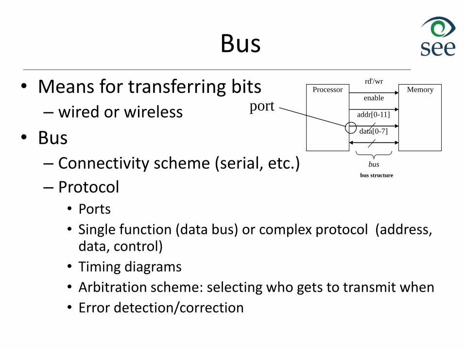
Bus

bus structure

Processor Memoryrd'/wr

enable

addr[0-11]

data[0-7]

bus

• Means for transferring bits– wired or wireless

• Bus– Connectivity scheme (serial, etc.)

– Protocol• Ports

• Single function (data bus) or complex protocol (address, data, control)

• Timing diagrams

• Arbitration scheme: selecting who gets to transmit when

• Error detection/correction

port

Error Detection & Correction

• Error detection: – Ability of receiver to detect errors during transmission

• Error correction: – Ability of receiver & transmitter to jointly correct the problem

• Parity: – Extra bit sent with word used for error detection

– Even/odd parity: data word plus parity bit transmitted

– Detects single bit errors, but not all burst bit errors

• Checksum: a count of the number of bits sent in transmission that can be used to check if all bits arrived

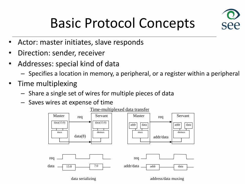
Basic Protocol Concepts• Actor: master initiates, slave responds

• Direction: sender, receiver

• Addresses: special kind of data– Specifies a location in memory, a peripheral, or a register within a peripheral

• Time multiplexing– Share a single set of wires for multiple pieces of data

– Saves wires at expense of time

data serializing address/data muxing

Master Servantreq

data(8)

data(15:0) data(15:0)

mux demux

Master Servantreq

addr/data

req

addr/data

addr data

mux demux

addr data

req

data 15:8 7:0 addr data

Time-multiplexed data transfer

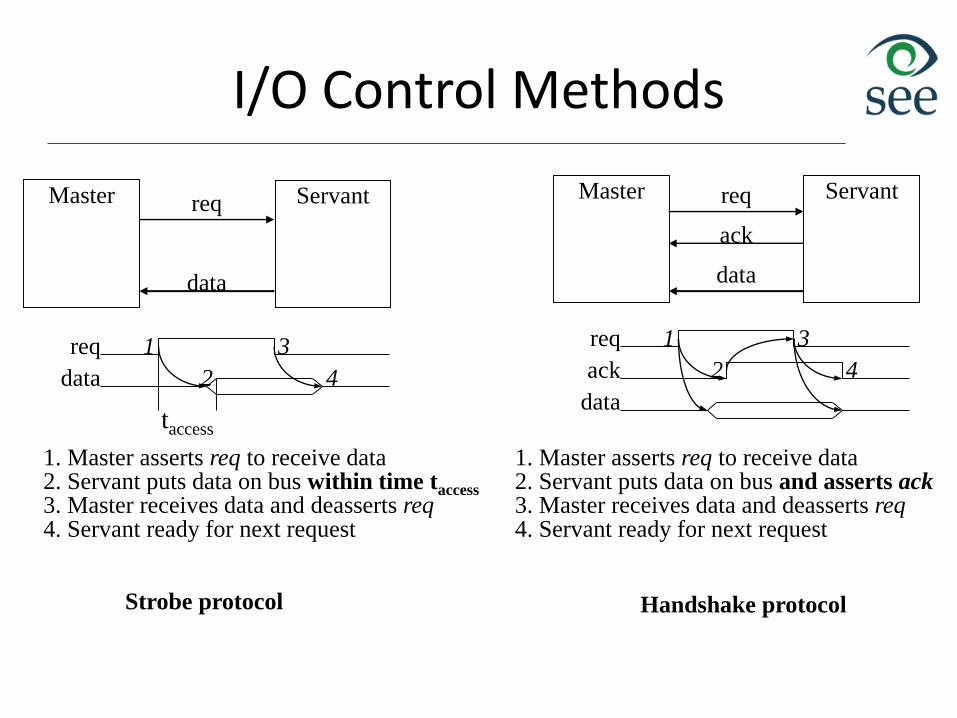
I/O Control Methods

Strobe protocol Handshake protocol

Master Servantreq

ack

req

data

Master Servant

data

req

data

taccess

req

data

ack

1. Master asserts req to receive data2. Servant puts data on bus within time taccess

1

2

3

4

3. Master receives data and deasserts req4. Servant ready for next request

1

2

3

4

1. Master asserts req to receive data2. Servant puts data on bus and asserts ack3. Master receives data and deasserts req4. Servant ready for next request

CPU Interface Methods

• Port-based I/O (parallel I/O)

– Processor has one or more N-bit ports

– Processor’s software reads and writes a port just like a register

• Bus-based I/O

– Processor has address, data and control ports that form a single bus

– Communication protocol is built into the processor

– A single instruction carries out the read or write protocol on the bus

Types of IO

• Two ways to talk to peripherals– Memory-mapped I/O

• Peripheral registers occupy addresses in the same address space as memory

• To access I/O use load/store instructions

– Standard I/O (I/O-mapped I/O)• Additional pin (M/IO) on bus indicates whether a

memory or peripheral access

• Special purpose instructions to access – e.g. Intel x86 provides in & out instructions

• Most CPUs use memory-mapped I/O

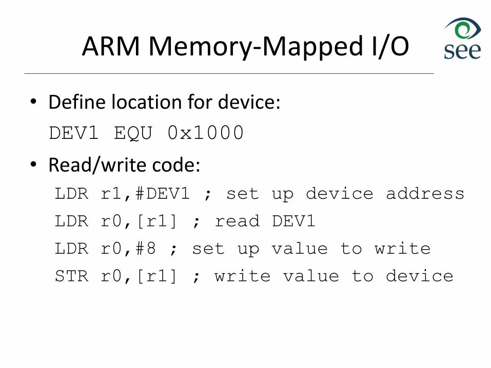
ARM Memory-Mapped I/O

• Define location for device:

DEV1 EQU 0x1000

• Read/write code:LDR r1,#DEV1 ; set up device address

LDR r0,[r1] ; read DEV1

LDR r0,#8 ; set up value to write

STR r0,[r1] ; write value to device

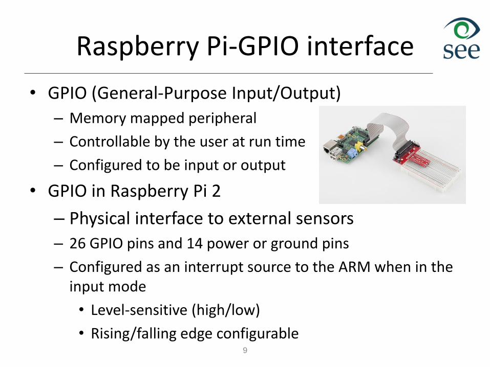
Raspberry Pi-GPIO interface

• GPIO (General-Purpose Input/Output)

– Memory mapped peripheral

– Controllable by the user at run time

– Configured to be input or output

• GPIO in Raspberry Pi 2

– Physical interface to external sensors

– 26 GPIO pins and 14 power or ground pins

– Configured as an interrupt source to the ARM when in the input mode

• Level-sensitive (high/low)

• Rising/falling edge configurable9

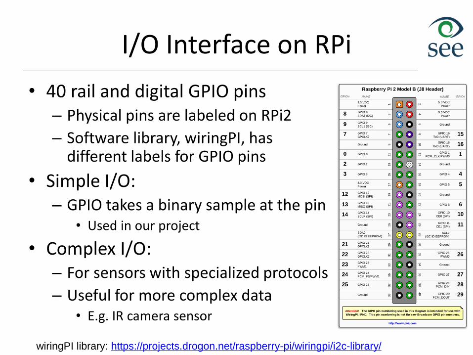
I/O Interface on RPi

• 40 rail and digital GPIO pins– Physical pins are labeled on RPi2

– Software library, wiringPI, has different labels for GPIO pins

• Simple I/O:– GPIO takes a binary sample at the pin

• Used in our project

• Complex I/O:– For sensors with specialized protocols

– Useful for more complex data • E.g. IR camera sensor

wiringPI library: https://projects.drogon.net/raspberry-pi/wiringpi/i2c-library/

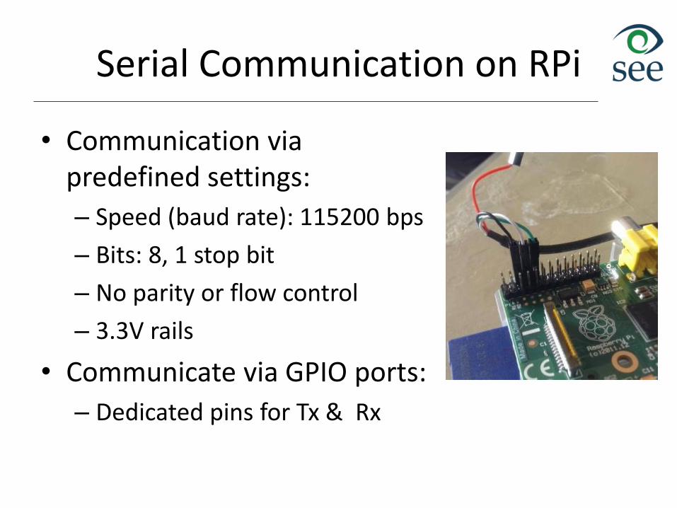
Serial Communication on RPi

• Communication via predefined settings:

– Speed (baud rate): 115200 bps

– Bits: 8, 1 stop bit

– No parity or flow control

– 3.3V rails

• Communicate via GPIO ports:

– Dedicated pins for Tx & Rx

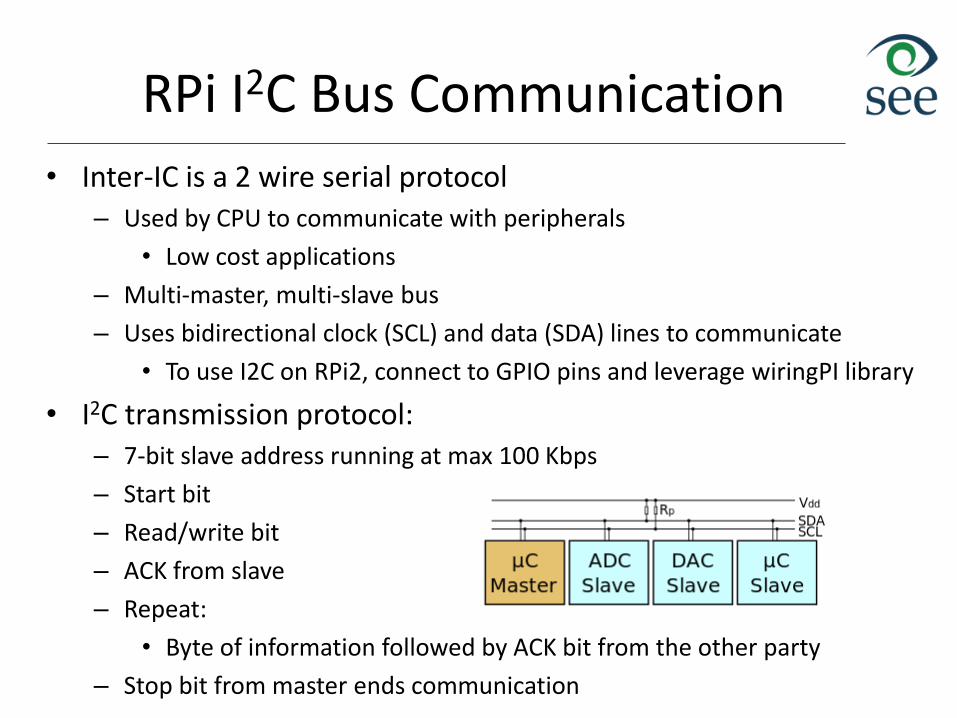
RPi I2C Bus Communication

• Inter-IC is a 2 wire serial protocol – Used by CPU to communicate with peripherals

• Low cost applications

– Multi-master, multi-slave bus

– Uses bidirectional clock (SCL) and data (SDA) lines to communicate

• To use I2C on RPi2, connect to GPIO pins and leverage wiringPI library

• I2C transmission protocol:– 7-bit slave address running at max 100 Kbps

– Start bit

– Read/write bit

– ACK from slave

– Repeat:

• Byte of information followed by ACK bit from the other party

– Stop bit from master ends communication

Polling vs Interrupts

• Polling– Peripheral intermittently receives data which must be

serviced by the processor

– CPU polls to check for data• It is very inefficient

• Hard to do simultaneous I/O

• Interrupt-driven I/O– Extra pin: if is 1, CPU jumps to ISR

– “polling” of the interrupt pin is built-into the hardware, so no extra time taken!

Priorities and vectors

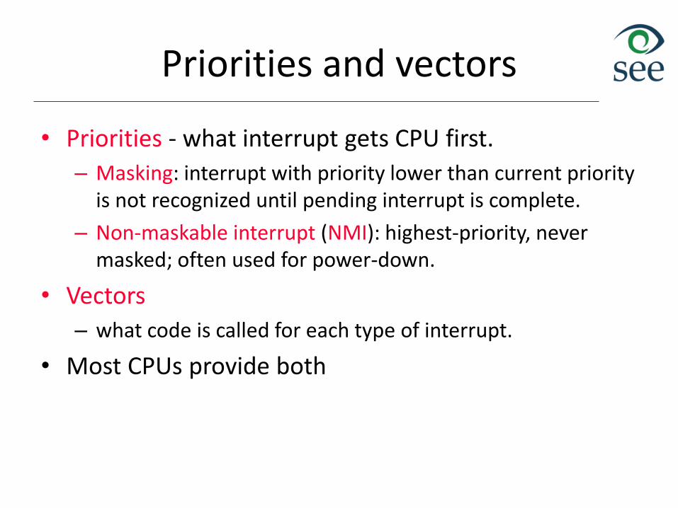
• Priorities - what interrupt gets CPU first.

– Masking: interrupt with priority lower than current priority is not recognized until pending interrupt is complete.

– Non-maskable interrupt (NMI): highest-priority, never masked; often used for power-down.

• Vectors

– what code is called for each type of interrupt.

• Most CPUs provide both

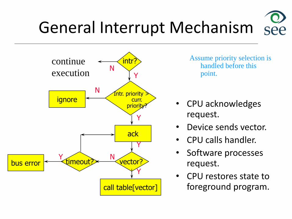
General Interrupt Mechanism

intr?N

Y

Assume priority selection is handled before this point.

N

ignore

Y

ack

vector?

Y

Y

Ntimeout?

Ybus error

call table[vector]

Intr. priority > curr.

priority?

continue

execution

• CPU acknowledges request.

• Device sends vector.

• CPU calls handler.

• Software processes request.

• CPU restores state to foreground program.

Sources of interrupt overhead

• Handler execution time.

• Interrupt mechanism overhead.

• Register save/restore.

• Pipeline-related penalties.

• Cache-related penalties.

Direct Memory Access

• Buffering– Temporarily storing data in memory before processing

• Microprocessor could handle this with ISR– Storing and restoring microprocessor state inefficient

– Regular program must wait

• DMA controller more efficient– Separate single-purpose processor

– Microprocessor relinquishes control of system bus to DMA controller

– Microprocessor can meanwhile execute its regular program

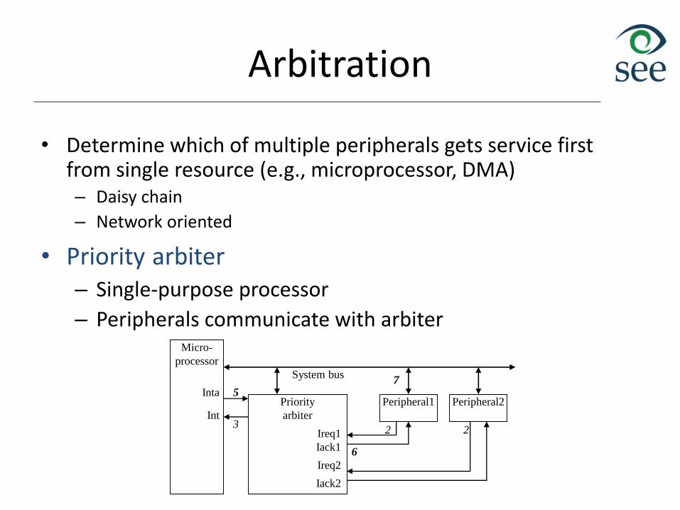
Arbitration

• Determine which of multiple peripherals gets service first from single resource (e.g., microprocessor, DMA)– Daisy chain

– Network oriented

• Priority arbiter– Single-purpose processor

– Peripherals communicate with arbiterMicro-

processor

Priority

arbiter

Peripheral1

System bus

Int3

57

IntaPeripheral2

Ireq1

Iack2

Iack1

Ireq2

2 2

6

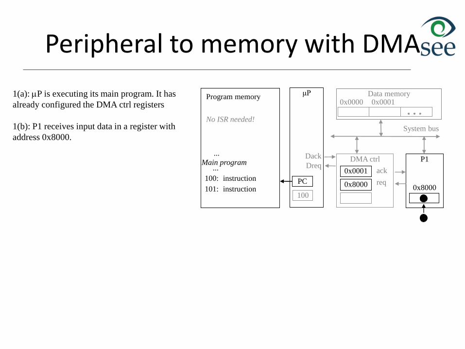
Peripheral to memory with DMA

1(a): P is executing its main program. It has

already configured the DMA ctrl registers

1(b): P1 receives input data in a register with

address 0x8000.

Data memoryμP

DMA ctrl P1

System bus

0x8000101:

instruction

instruction

...

Main program...

Program memory

PC

100

Dreq

Dack

0x0000 0x0001

100:

No ISR needed!

0x0001

0x8000

ack

req

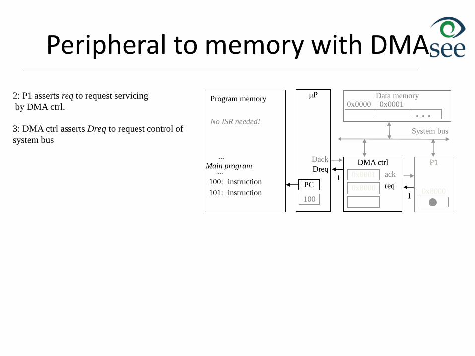
Peripheral to memory with DMA

2: P1 asserts req to request servicing

by DMA ctrl.

3: DMA ctrl asserts Dreq to request control of

system bus

Data memoryμP

DMA ctrl P1

System bus

0x8000101:

instruction

instruction

...

Main program...

Program memory

PC

100

Dreq

Dack

0x0000 0x0001

100:

No ISR needed!

0x0001

0x8000

ack

reqreq

1

P1Dreq

1

DMA ctrl P1

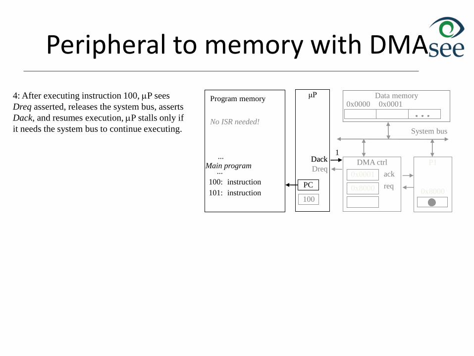
Peripheral to memory with DMA

4: After executing instruction 100, P sees

Dreq asserted, releases the system bus, asserts

Dack, and resumes execution, P stalls only if

it needs the system bus to continue executing.

Data memoryμP

DMA ctrl P1

System bus

0x8000101:

instruction

instruction

...

Main program...

Program memory

PC

100

Dreq

Dack

0x0000 0x0001

100:

No ISR needed!

0x0001

0x8000

ack

req

Dack1

Data memoryμP

DMA ctrl P1

System bus

0x8000101:

instruction

instruction

...

Main program...

Program memory

PC

100

Dreq

Dack

0x0000 0x0001

100:

No ISR needed!

0x0001

0x8000

ack

req

Data memory

DMA ctrl P1

System bus

0x8000

0x0000 0x0001

0x0001

0x8000

ack

req

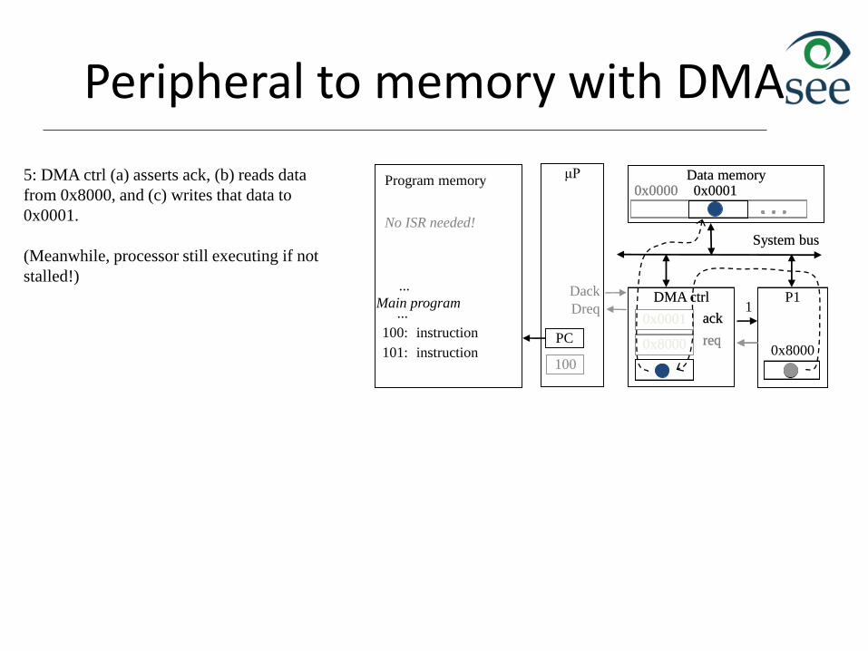
Peripheral to memory with DMA

5: DMA ctrl (a) asserts ack, (b) reads data

from 0x8000, and (c) writes that data to

0x0001.

(Meanwhile, processor still executing if not

stalled!)

ack1

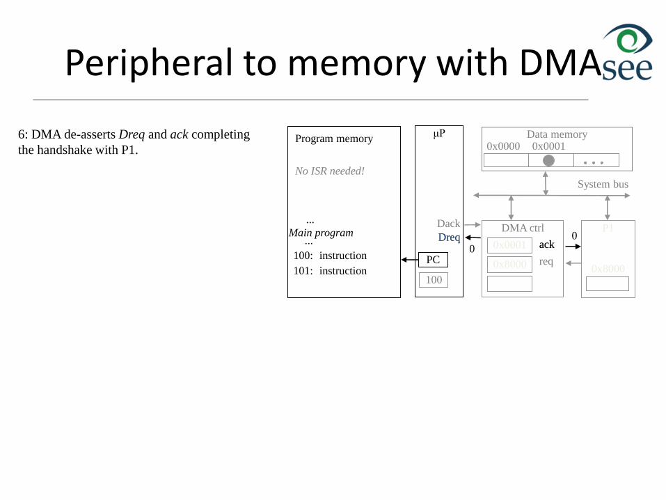
Peripheral to memory with DMA

6: DMA de-asserts Dreq and ack completing

the handshake with P1.

Data memoryμP

DMA ctrl P1

System bus

0x8000101:

instruction

instruction

...

Main program...

Program memory

PC

100

Dreq

Dack

0x0000 0x0001

100:

No ISR needed!

0x0001

0x8000

ack

req

ack0Dreq

0

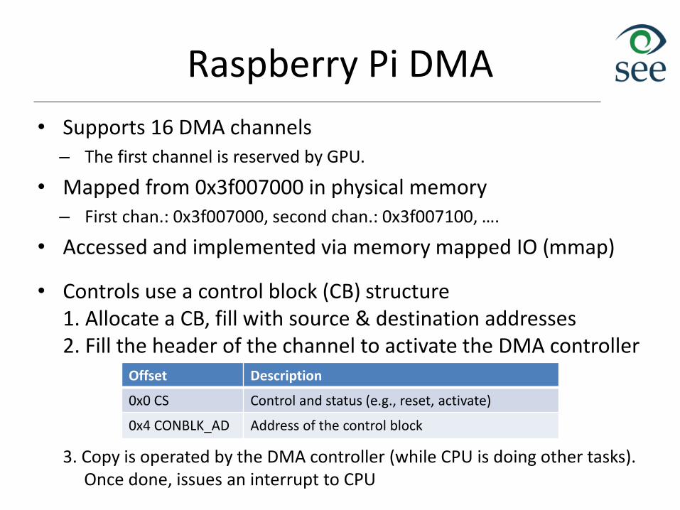
Raspberry Pi DMA

• Supports 16 DMA channels– The first channel is reserved by GPU.

• Mapped from 0x3f007000 in physical memory– First chan.: 0x3f007000, second chan.: 0x3f007100, ….

• Accessed and implemented via memory mapped IO (mmap)

• Controls use a control block (CB) structure1. Allocate a CB, fill with source & destination addresses2. Fill the header of the channel to activate the DMA controller

3. Copy is operated by the DMA controller (while CPU is doing other tasks).Once done, issues an interrupt to CPU

Offset Description

0x0 CS Control and status (e.g., reset, activate)

0x4 CONBLK_AD Address of the control block

ADC & DAC

Tajana Simunic Rosing

Department of Computer Science and Engineering

University of California, San Diego.

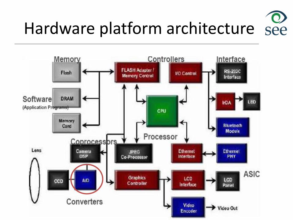
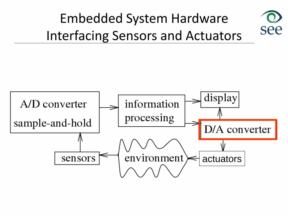
Hardware platform architecture

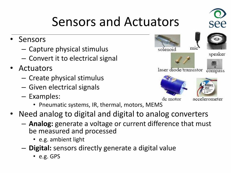
Sensors and Actuators• Sensors

– Capture physical stimulus– Convert it to electrical signal

• Actuators– Create physical stimulus – Given electrical signals– Examples:

• Pneumatic systems, IR, thermal, motors, MEMS

• Need analog to digital and digital to analog converters– Analog: generate a voltage or current difference that must

be measured and processed• e.g. ambient light

– Digital: sensors directly generate a digital value• e.g. GPS

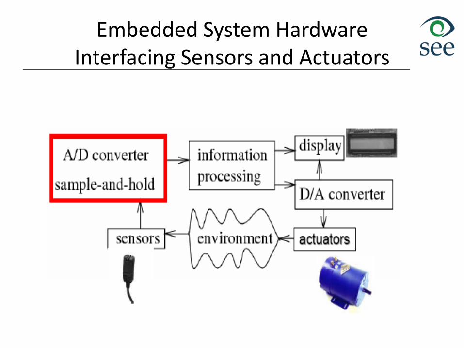
Embedded System HardwareInterfacing Sensors and Actuators

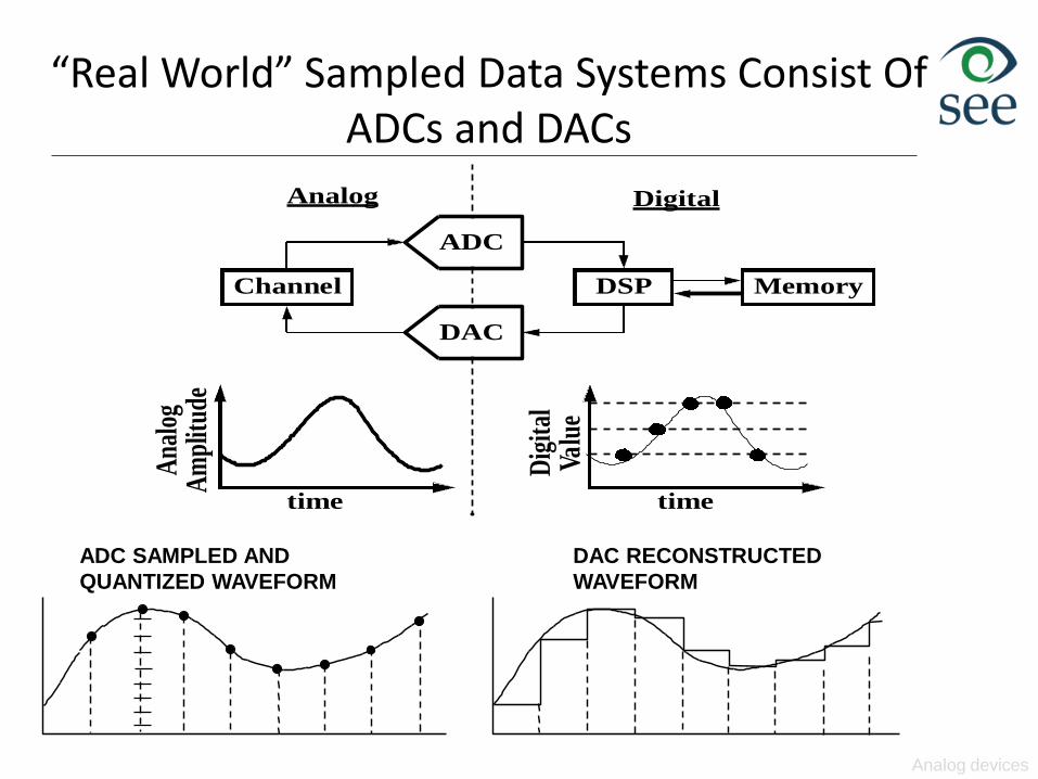
ADC SAMPLED AND

QUANTIZED WAVEFORM

DAC RECONSTRUCTED

WAVEFORM

ADC

DAC

DSP MemoryChannel

Analog Digital

timetime

Ana

log

Dig

ital

Am

plit

ude

Valu

e

“Real World” Sampled Data Systems Consist Of ADCs and DACs

Analog devices

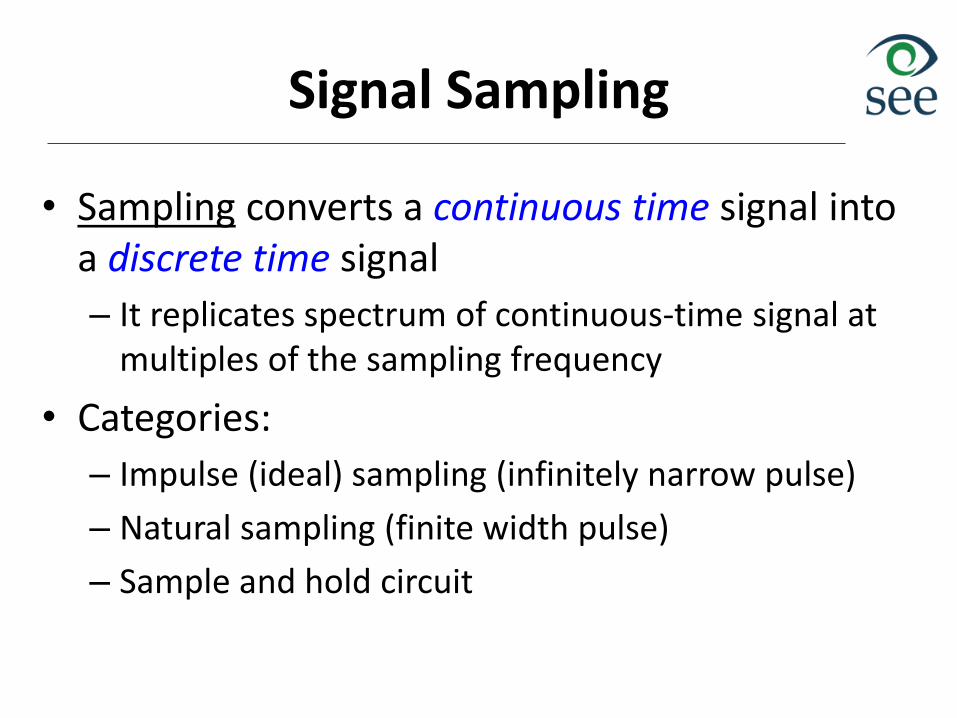
Signal Sampling

• Sampling converts a continuous time signal into a discrete time signal

– It replicates spectrum of continuous-time signal at multiples of the sampling frequency

• Categories:

– Impulse (ideal) sampling (infinitely narrow pulse)

– Natural sampling (finite width pulse)

– Sample and hold circuit

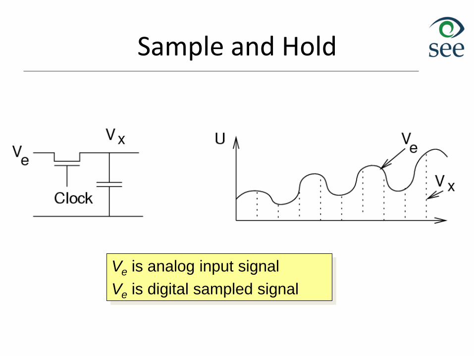
Sample and Hold

Ve is analog input signal

Ve is digital sampled signal

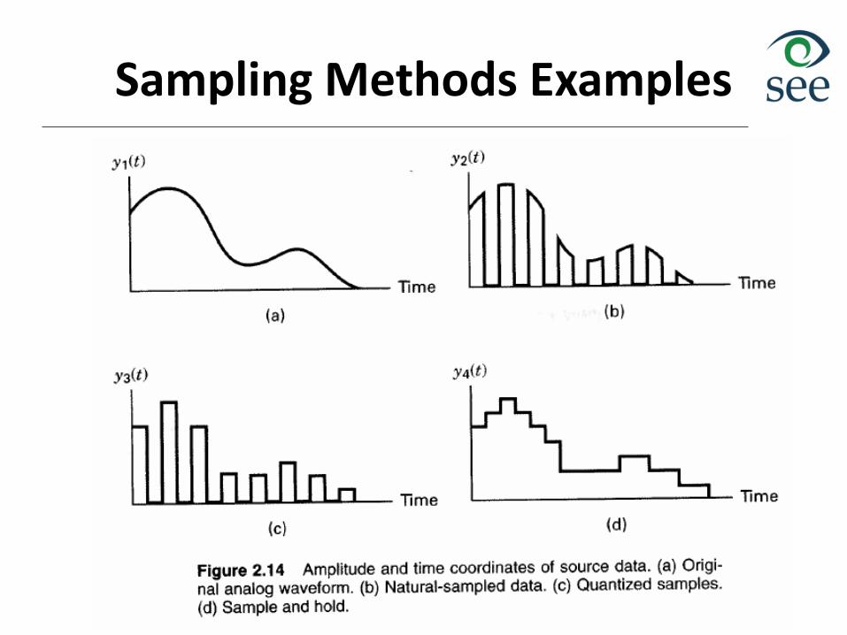
Sampling Methods Examples

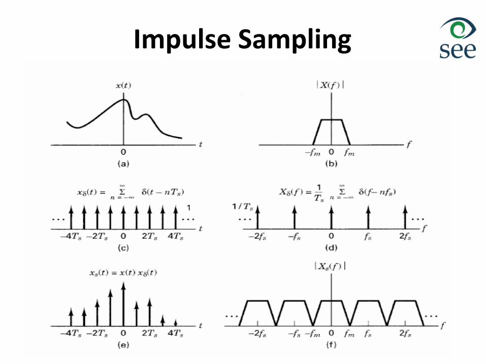
Impulse Sampling

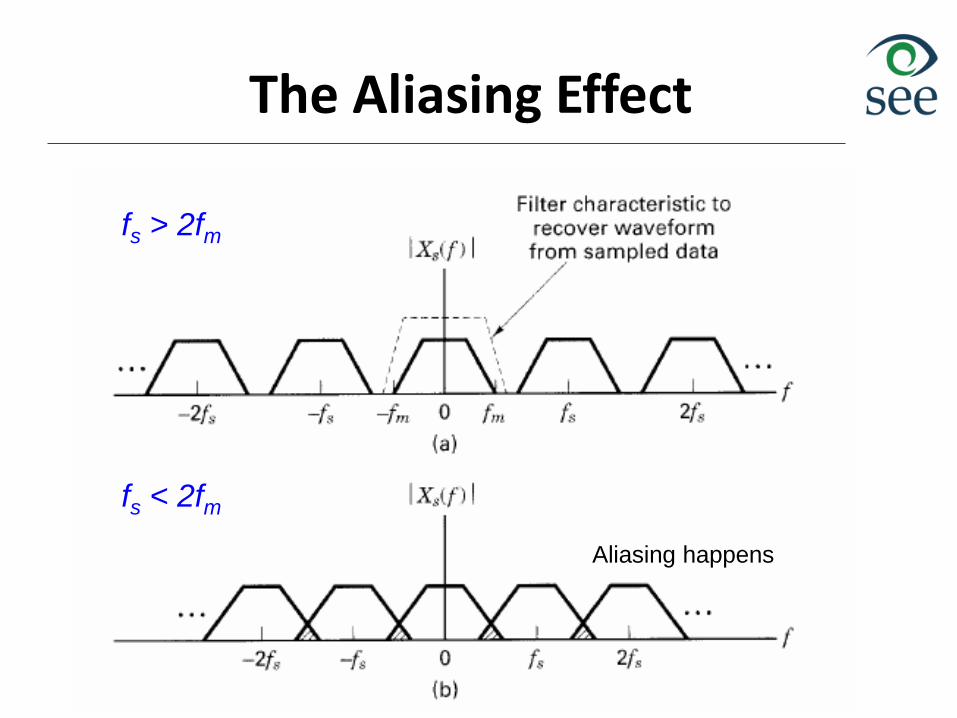
The Aliasing Effect

fs > 2fm

fs < 2fm

Aliasing happens

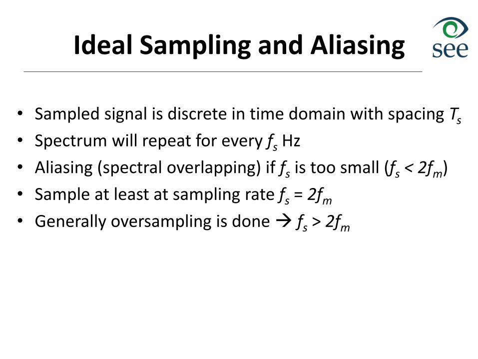
Ideal Sampling and Aliasing

• Sampled signal is discrete in time domain with spacing Ts

• Spectrum will repeat for every fs Hz

• Aliasing (spectral overlapping) if fs is too small (fs < 2fm)

• Sample at least at sampling rate fs = 2fm

• Generally oversampling is done fs > 2fm

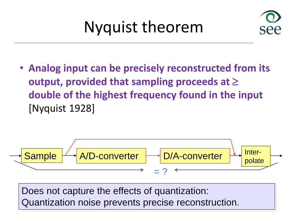
Nyquist theorem

• Analog input can be precisely reconstructed from its output, provided that sampling proceeds at double of the highest frequency found in the input [Nyquist 1928]

Sample A/D-converter D/A-converter

= ?

Inter-

polate

Does not capture the effects of quantization:

Quantization noise prevents precise reconstruction.

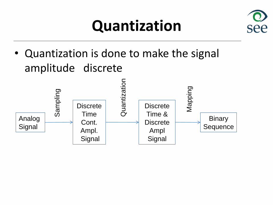
Quantization

• Quantization is done to make the signal amplitude discrete

Analog

Signal

Sam

plin

g

Discrete

Time

Cont.

Ampl.

Signal

Qu

antization

Discrete

Time &

Discrete

Ampl

Signal

Mappin

g

Binary

Sequence

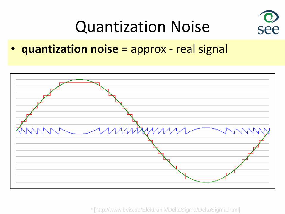
Quantization Noise• quantization noise = approx - real signal

* [http://www.beis.de/Elektronik/DeltaSigma/DeltaSigma.html]

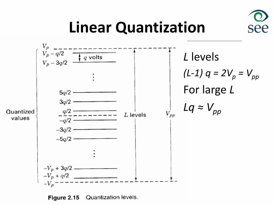
Linear Quantization

L levels

(L-1) q = 2Vp = Vpp

For large L

Lq ≈ Vpp

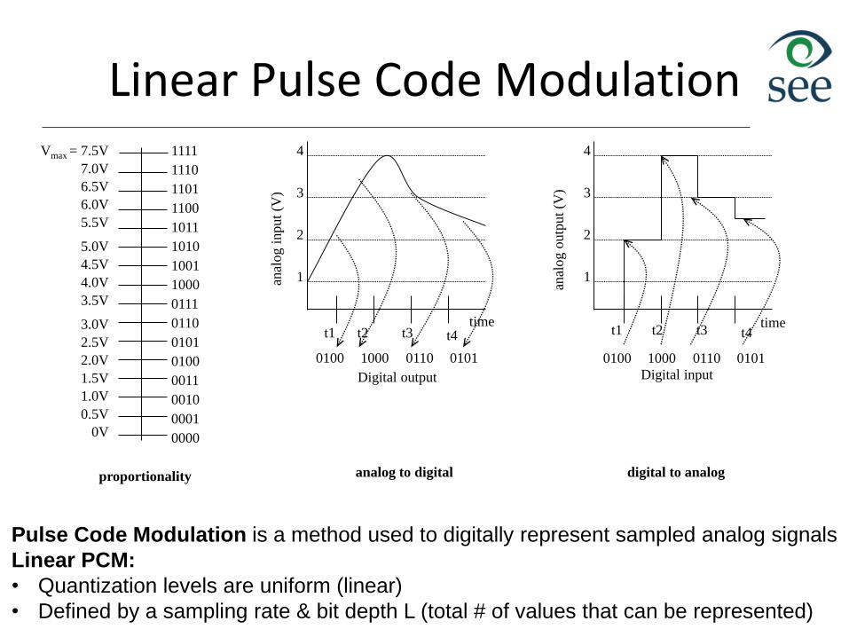
Linear Pulse Code Modulation

proportionality

Vmax = 7.5V

0V

1111

1110

0000

0010

0100

0110

1000

1010

1100

0001

0011

0101

0111

1001

1011

1101

0.5V

1.0V

1.5V

2.0V

2.5V

3.0V

3.5V

4.0V

4.5V

5.0V

5.5V

6.0V

6.5V

7.0V

analog to digital

4

3

2

1

t1 t2 t3 t4

0100 1000 0110 0101

time

anal

og i

nput

(V)

Digital output

digital to analog

4

3

2

1

0100 1000 0110 0101

t1 t2 t3 t4time

anal

og o

utp

ut

(V)

Digital input

Pulse Code Modulation is a method used to digitally represent sampled analog signals

Linear PCM:

• Quantization levels are uniform (linear)

• Defined by a sampling rate & bit depth L (total # of values that can be represented)

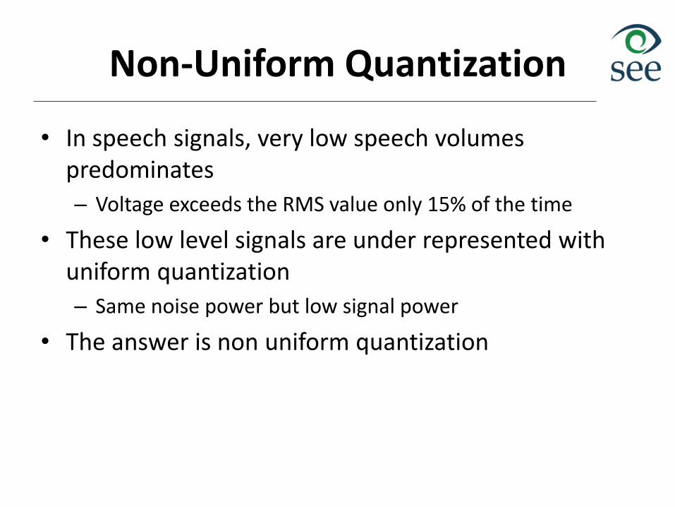
Non-Uniform Quantization

• In speech signals, very low speech volumes predominates

– Voltage exceeds the RMS value only 15% of the time

• These low level signals are under represented with uniform quantization

– Same noise power but low signal power

• The answer is non uniform quantization

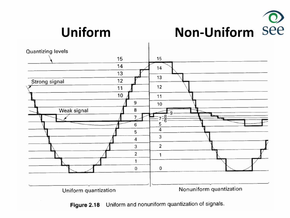
Uniform Non-Uniform

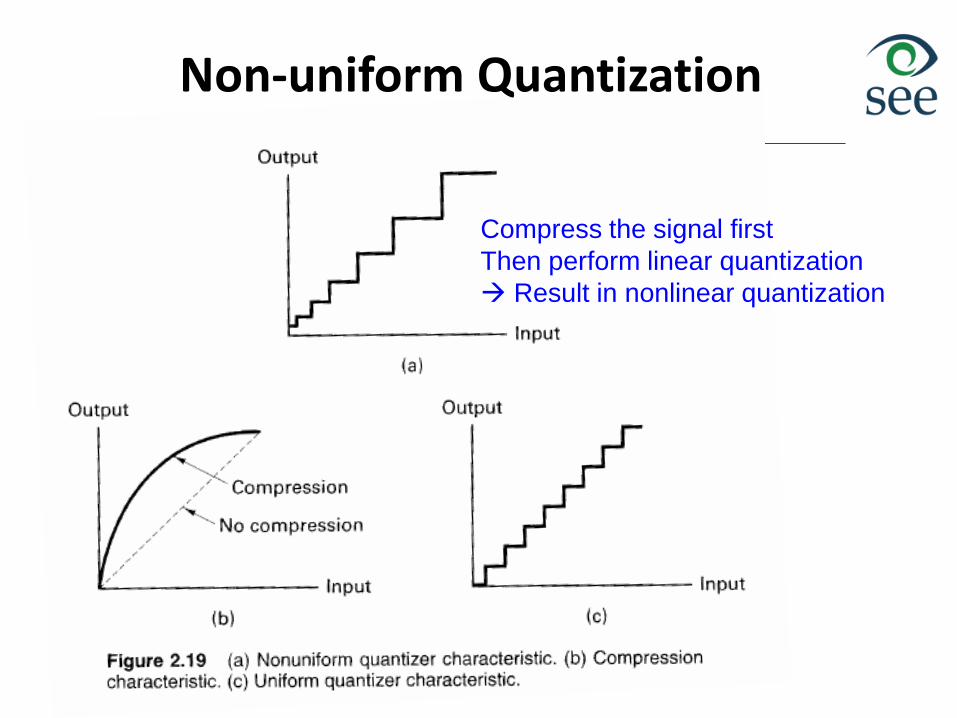
Non-uniform Quantization

Compress the signal first

Then perform linear quantization

Result in nonlinear quantization

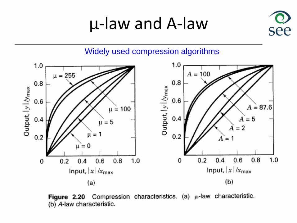
µ-law and A-law

Widely used compression algorithms

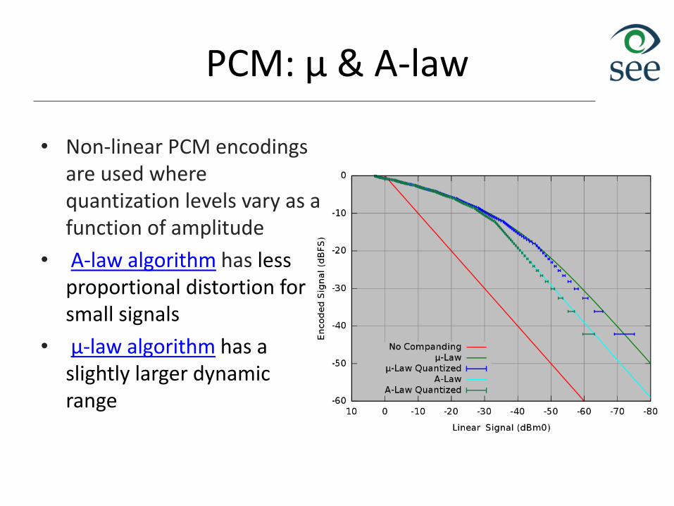
PCM: µ & A-law

• Non-linear PCM encodings are used where quantization levels vary as a function of amplitude

• A-law algorithm has less proportional distortion for small signals

• μ-law algorithm has a slightly larger dynamic range

actuators

Embedded System HardwareInterfacing Sensors and Actuators

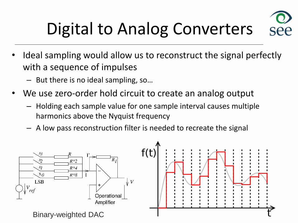
Digital to Analog Converters

• Ideal sampling would allow us to reconstruct the signal perfectly with a sequence of impulses– But there is no ideal sampling, so…

• We use zero-order hold circuit to create an analog output – Holding each sample value for one sample interval causes multiple

harmonics above the Nyquist frequency

– A low pass reconstruction filter is needed to recreate the signal

Binary-weighted DAC

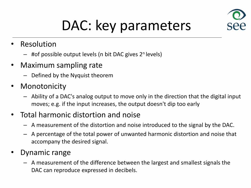
DAC: key parameters• Resolution

– #of possible output levels (n bit DAC gives 2n levels)

• Maximum sampling rate– Defined by the Nyquist theorem

• Monotonicity– Ability of a DAC's analog output to move only in the direction that the digital input

moves; e.g. if the input increases, the output doesn't dip too early

• Total harmonic distortion and noise – A measurement of the distortion and noise introduced to the signal by the DAC.

– A percentage of the total power of unwanted harmonic distortion and noise that accompany the desired signal.

• Dynamic range– A measurement of the difference between the largest and smallest signals the

DAC can reproduce expressed in decibels.

System Energy Efficiency Lab

seelab.ucsd.edu

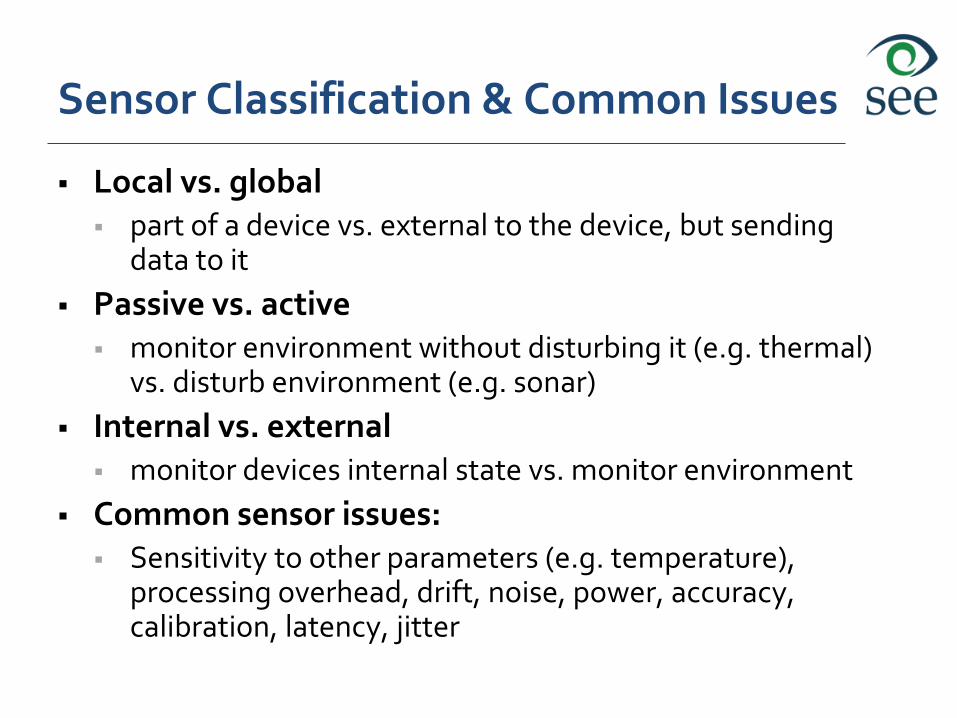
Sensor Classification & Common Issues

Local vs. global part of a device vs. external to the device, but sending

data to it

Passive vs. active monitor environment without disturbing it (e.g. thermal)

vs. disturb environment (e.g. sonar)

Internal vs. external monitor devices internal state vs. monitor environment

Common sensor issues: Sensitivity to other parameters (e.g. temperature),

processing overhead, drift, noise, power, accuracy, calibration, latency, jitter

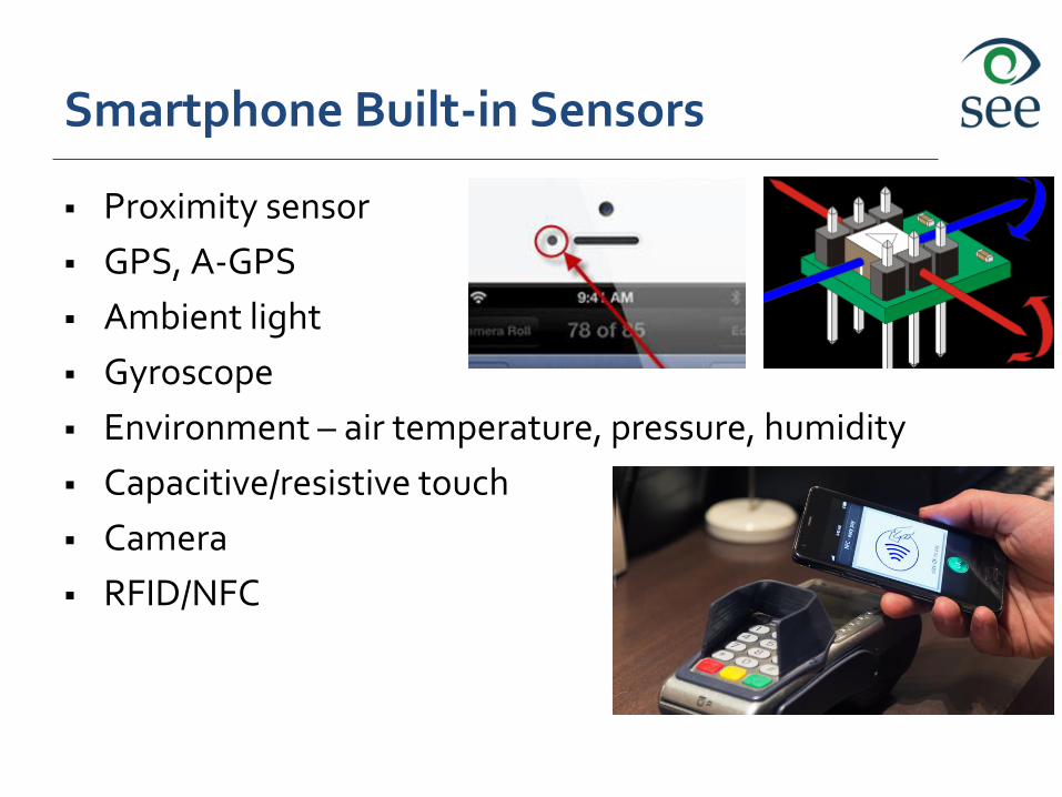
Smartphone Built-in Sensors

Proximity sensor

GPS, A-GPS

Ambient light

Gyroscope

Environment – air temperature, pressure, humidity

Capacitive/resistive touch

Camera

RFID/NFC

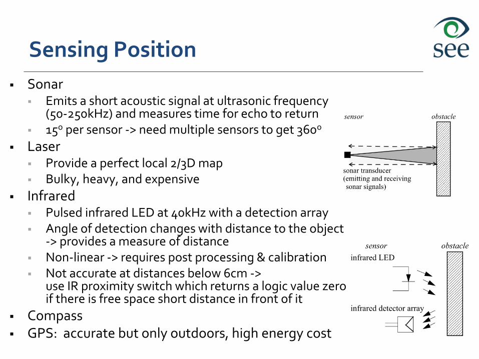
Sensing Position

Sonar Emits a short acoustic signal at ultrasonic frequency

(50-250kHz) and measures time for echo to return 15o per sensor -> need multiple sensors to get 360o

Laser Provide a perfect local 2/3D map Bulky, heavy, and expensive

Infrared Pulsed infrared LED at 40kHz with a detection array Angle of detection changes with distance to the object

-> provides a measure of distance Non-linear -> requires post processing & calibration Not accurate at distances below 6cm ->

use IR proximity switch which returns a logic value zero if there is free space short distance in front of it

Compass GPS: accurate but only outdoors, high energy cost

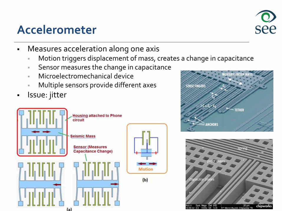
Accelerometer

Measures acceleration along one axis Motion triggers displacement of mass, creates a change in capacitance Sensor measures the change in capacitance Microelectromechanical device Multiple sensors provide different axes

Issue: jitter

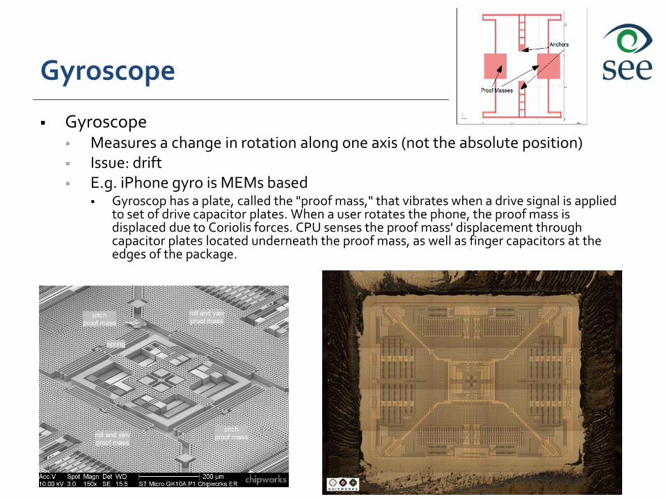
Gyroscope

Gyroscope Measures a change in rotation along one axis (not the absolute position) Issue: drift E.g. iPhone gyro is MEMs based

Gyroscop has a plate, called the "proof mass," that vibrates when a drive signal is applied to set of drive capacitor plates. When a user rotates the phone, the proof mass is displaced due to Coriolis forces. CPU senses the proof mass' displacement through capacitor plates located underneath the proof mass, as well as finger capacitors at the edges of the package.

Inclinometer

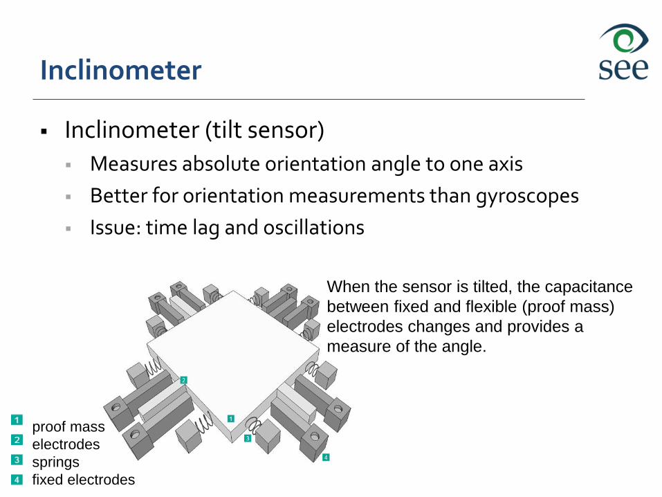
Inclinometer (tilt sensor)

Measures absolute orientation angle to one axis

Better for orientation measurements than gyroscopes

Issue: time lag and oscillations

When the sensor is tilted, the capacitance

between fixed and flexible (proof mass)

electrodes changes and provides a

measure of the angle.

proof mass

electrodes

springs

fixed electrodes

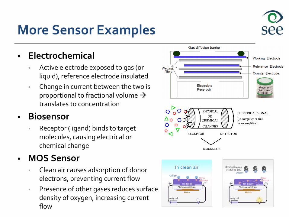
More Sensor Examples

Electrochemical Active electrode exposed to gas (or

liquid), reference electrode insulated

Change in current between the two is proportional to fractional volume translates to concentration

Biosensor Receptor (ligand) binds to target

molecules, causing electrical or chemical change

MOS Sensor Clean air causes adsorption of donor

electrons, preventing current flow

Presence of other gases reduces surface density of oxygen, increasing current flow

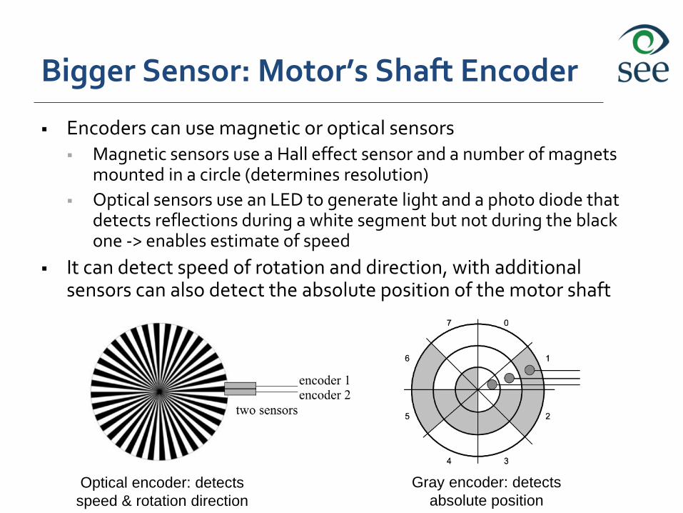
Bigger Sensor: Motor’s Shaft Encoder

Encoders can use magnetic or optical sensors Magnetic sensors use a Hall effect sensor and a number of magnets

mounted in a circle (determines resolution)

Optical sensors use an LED to generate light and a photo diode that detects reflections during a white segment but not during the black one -> enables estimate of speed

It can detect speed of rotation and direction, with additional sensors can also detect the absolute position of the motor shaft

Optical encoder: detects

speed & rotation direction

Gray encoder: detects

absolute position

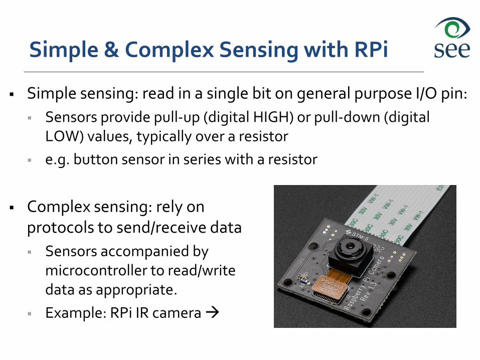
Simple & Complex Sensing with RPi

Simple sensing: read in a single bit on general purpose I/O pin:

Sensors provide pull-up (digital HIGH) or pull-down (digital LOW) values, typically over a resistor

e.g. button sensor in series with a resistor

Complex sensing: rely on protocols to send/receive data

Sensors accompanied by microcontroller to read/write data as appropriate.

Example: RPi IR camera

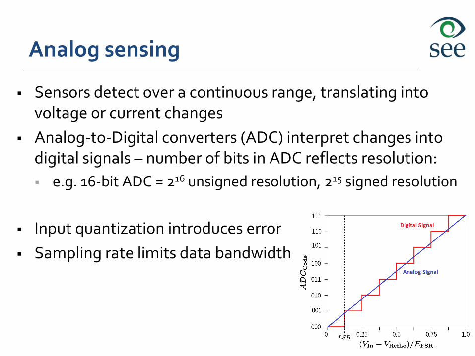
Analog sensing

Sensors detect over a continuous range, translating into voltage or current changes

Analog-to-Digital converters (ADC) interpret changes into digital signals – number of bits in ADC reflects resolution:

e.g. 16-bit ADC = 216 unsigned resolution, 215 signed resolution

Input quantization introduces error

Sampling rate limits data bandwidth

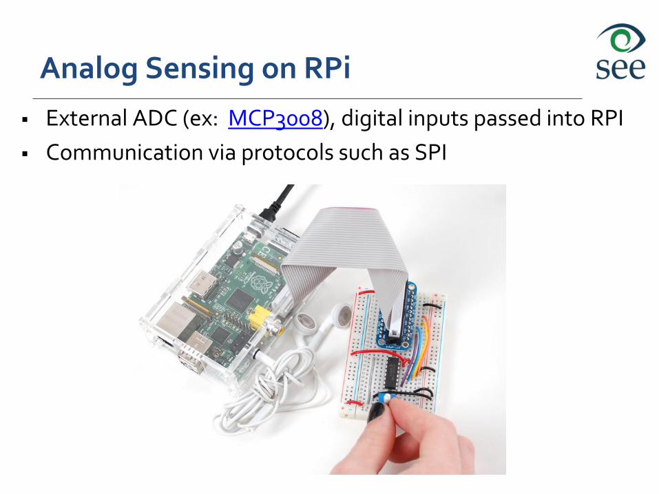
Analog Sensing on RPi

External ADC (ex: MCP3008), digital inputs passed into RPI

Communication via protocols such as SPI

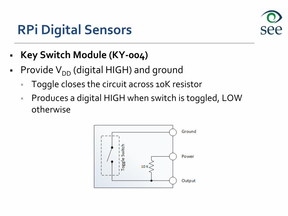
RPi Digital Sensors

Key Switch Module (KY-004)

Provide VDD (digital HIGH) and ground

Toggle closes the circuit across 10K resistor

Produces a digital HIGH when switch is toggled, LOW otherwise

RPi Digital Sensors

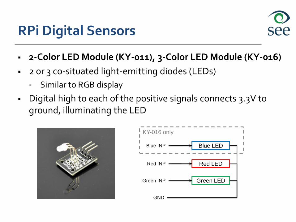
2-Color LED Module (KY-011), 3-Color LED Module (KY-016)

2 or 3 co-situated light-emitting diodes (LEDs)

Similar to RGB display

Digital high to each of the positive signals connects 3.3V to ground, illuminating the LED

Blue LED

Red LED

Green LED

Red INP

Green INP

GND

Blue INP

KY-016 only

RPi Digital Sensors

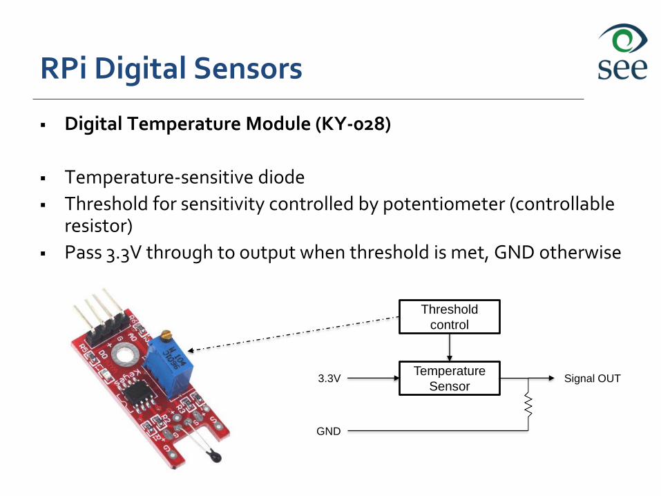
Digital Temperature Module (KY-028)

Temperature-sensitive diode

Threshold for sensitivity controlled by potentiometer (controllable resistor)

Pass 3.3V through to output when threshold is met, GND otherwise

Temperature

Sensor3.3V

GND

Threshold

control

Signal OUT

RPi Digital Sensors

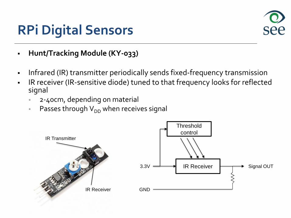
Hunt/Tracking Module (KY-033)

Infrared (IR) transmitter periodically sends fixed-frequency transmission IR receiver (IR-sensitive diode) tuned to that frequency looks for reflected

signal 2-40cm, depending on material Passes through VDD when receives signal

IR Transmitter

IR Receiver

IR Receiver3.3V

GND

Threshold

control

Signal OUT

RPi Digital Sensors

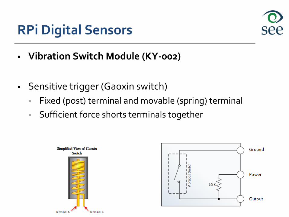
Vibration Switch Module (KY-002)

Sensitive trigger (Gaoxin switch)

Fixed (post) terminal and movable (spring) terminal

Sufficient force shorts terminals together

RPi Digital Sensors

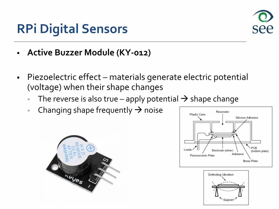
Active Buzzer Module (KY-012)

Piezoelectric effect – materials generate electric potential (voltage) when their shape changes The reverse is also true – apply potential shape change

Changing shape frequently noise

TCN75A:Analog Sensor with a built-in ADC

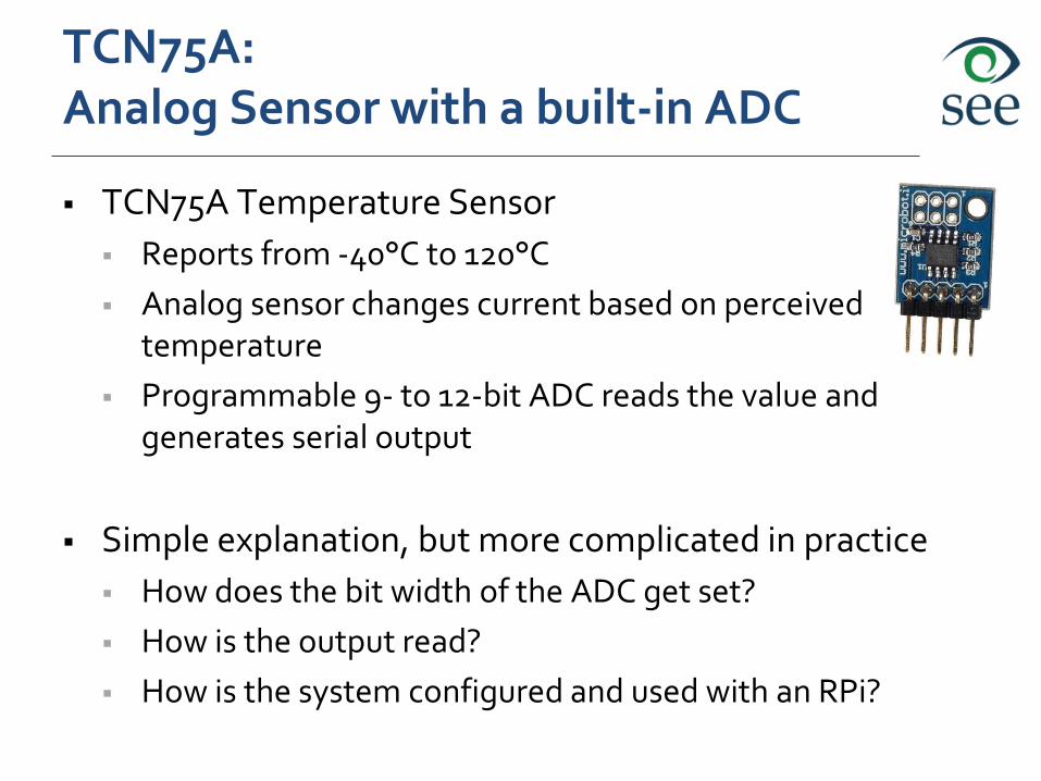
TCN75A Temperature Sensor

Reports from -40°C to 120°C

Analog sensor changes current based on perceivedtemperature

Programmable 9- to 12-bit ADC reads the value and generates serial output

Simple explanation, but more complicated in practice

How does the bit width of the ADC get set?

How is the output read?

How is the system configured and used with an RPi?

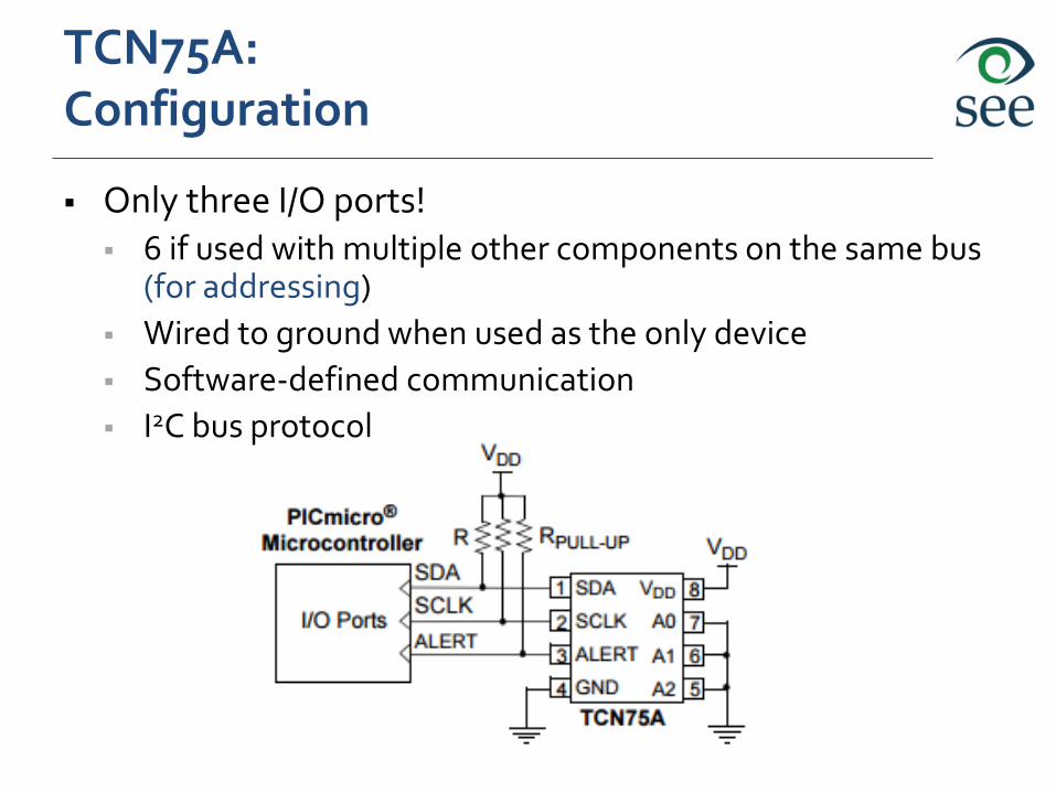
TCN75A: Configuration

Only three I/O ports! 6 if used with multiple other components on the same bus

(for addressing)

Wired to ground when used as the only device

Software-defined communication

I2C bus protocol

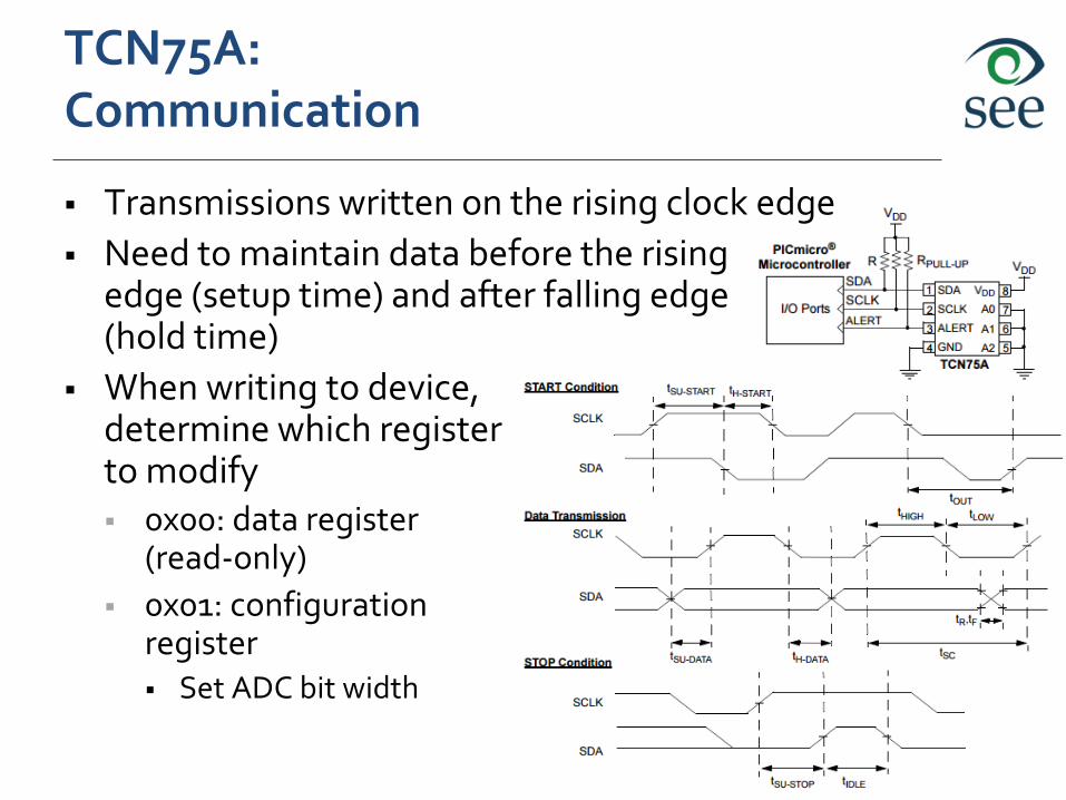
TCN75A: Communication

Transmissions written on the rising clock edge

Need to maintain data before the risingedge (setup time) and after falling edge (hold time)

When writing to device,determine which registerto modify 0x00: data register

(read-only)

0x01: configurationregister Set ADC bit width

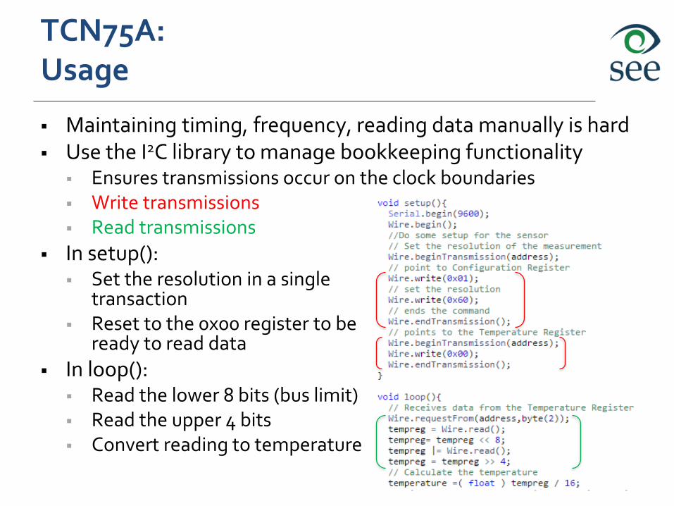
TCN75A: Usage

Maintaining timing, frequency, reading data manually is hard Use the I2C library to manage bookkeeping functionality

Ensures transmissions occur on the clock boundaries Write transmissions Read transmissions

In setup(): Set the resolution in a single

transaction Reset to the 0x00 register to be

ready to read data

In loop(): Read the lower 8 bits (bus limit) Read the upper 4 bits Convert reading to temperature

Actuators

Cause changes to the physical world

Can be as passive as changing screen elements, or keeping an aerial system aloft

Ensure stability/safety/reliability of the embedded system itself

Typically feedback loop (e.g. flight stability via PID controller)

MoC transitions/states can also trigger actuation

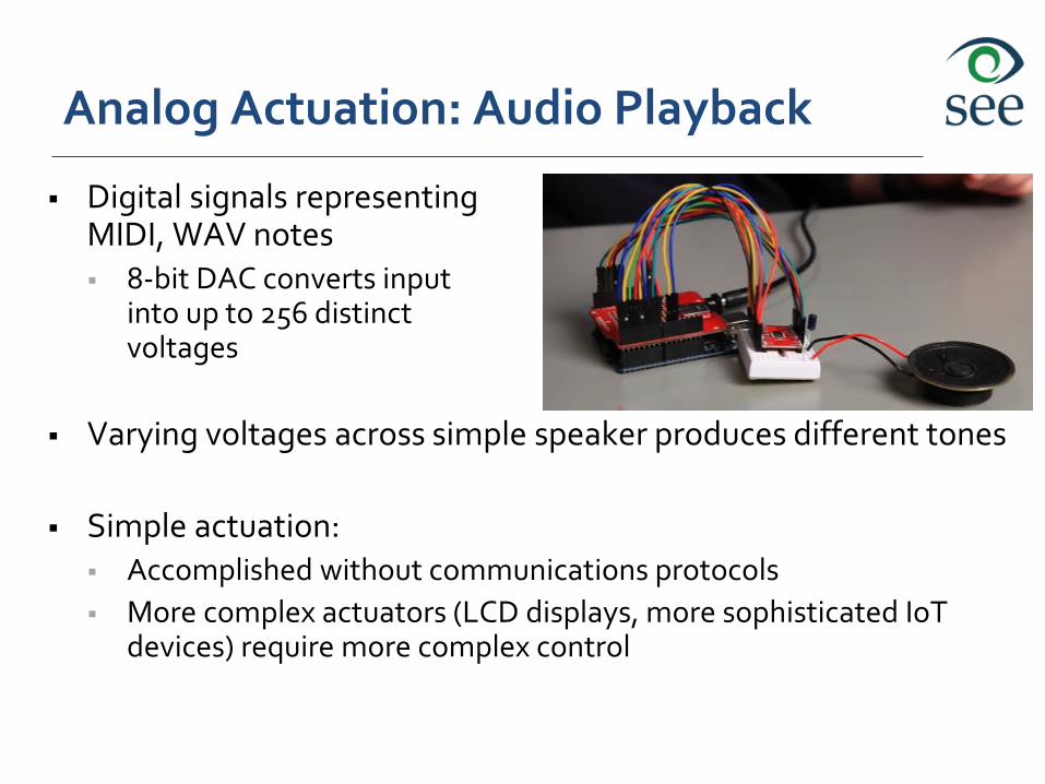
Analog Actuation: Audio Playback

Digital signals representing MIDI, WAV notes 8-bit DAC converts input

into up to 256 distinctvoltages

Varying voltages across simple speaker produces different tones

Simple actuation: Accomplished without communications protocols

More complex actuators (LCD displays, more sophisticated IoT devices) require more complex control

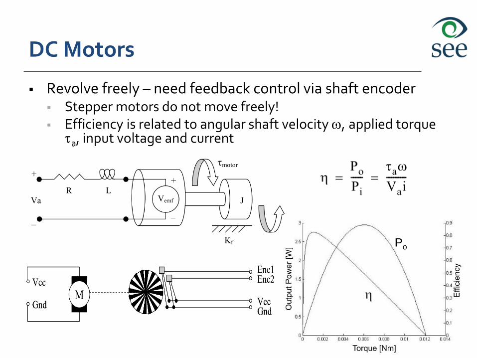
DC Motors

Revolve freely – need feedback control via shaft encoder Stepper motors do not move freely! Efficiency is related to angular shaft velocity w, applied torque

ta, input voltage and current

Po

h

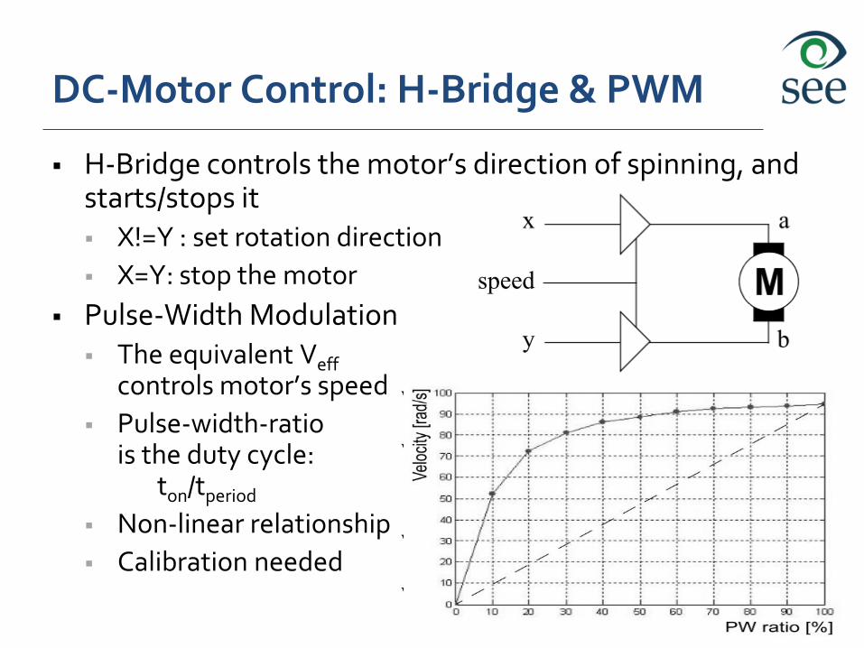
DC-Motor Control: H-Bridge & PWM

H-Bridge controls the motor’s direction of spinning, and starts/stops it X!=Y : set rotation direction

X=Y: stop the motor

Pulse-Width Modulation The equivalent Veff

controls motor’s speed

Pulse-width-ratiois the duty cycle:

ton/tperiod

Non-linear relationship

Calibration needed

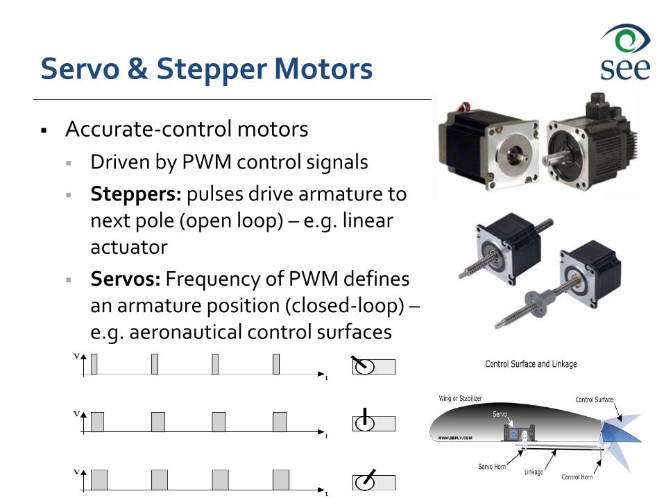
Servo & Stepper Motors

Accurate-control motors

Driven by PWM control signals

Steppers: pulses drive armature to next pole (open loop) – e.g. linear actuator

Servos: Frequency of PWM defines an armature position (closed-loop) –e.g. aeronautical control surfaces

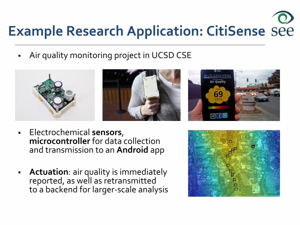
Example Research Application: CitiSense

Air quality monitoring project in UCSD CSE

Electrochemical sensors,microcontroller for data collectionand transmission to an Android app

Actuation: air quality is immediatelyreported, as well as retransmitted to a backend for larger-scale analysis

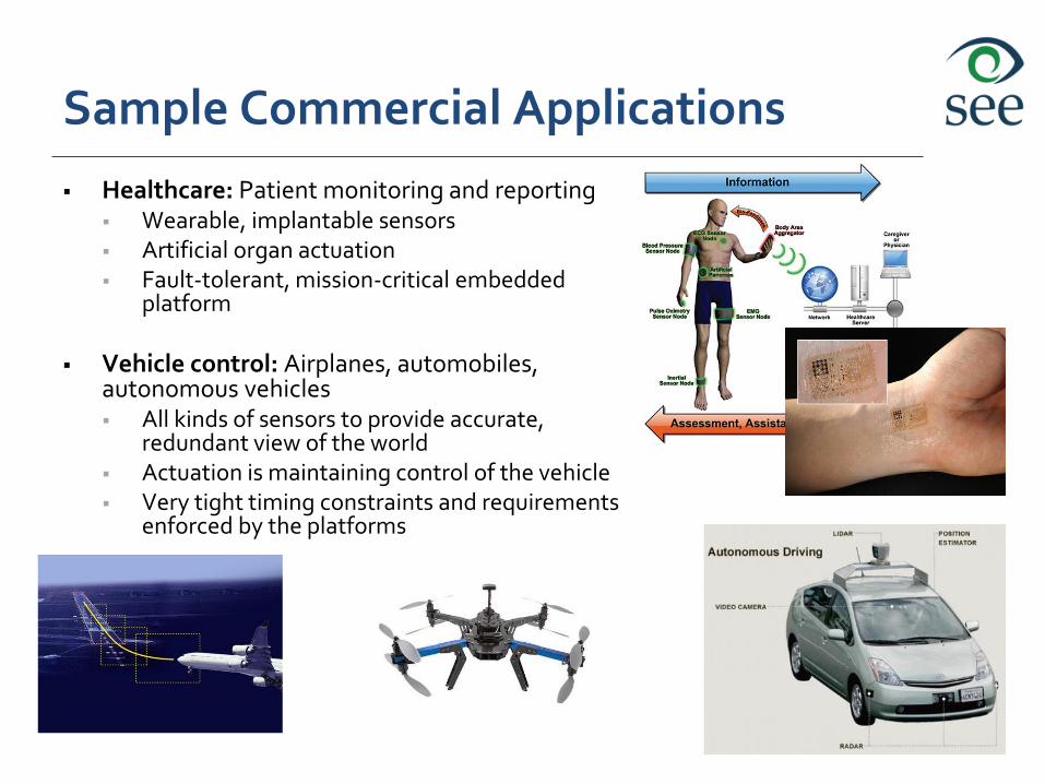
Sample Commercial Applications

Healthcare: Patient monitoring and reporting Wearable, implantable sensors Artificial organ actuation Fault-tolerant, mission-critical embedded

platform

Vehicle control: Airplanes, automobiles, autonomous vehicles All kinds of sensors to provide accurate,

redundant view of the world Actuation is maintaining control of the vehicle Very tight timing constraints and requirements

enforced by the platforms

Basics of Control

Tajana Simunic Rosing

Department of Computer Science and Engineering

University of California, San Diego.

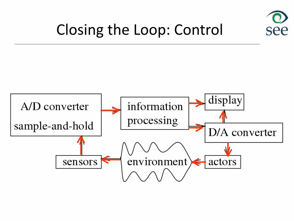
Closing the Loop: Control

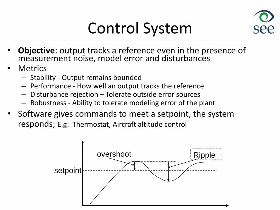
Control System• Objective: output tracks a reference even in the presence of

measurement noise, model error and disturbances• Metrics

– Stability - Output remains bounded– Performance - How well an output tracks the reference– Disturbance rejection – Tolerate outside error sources– Robustness - Ability to tolerate modeling error of the plant

• Software gives commands to meet a setpoint, the system responds; E.g: Thermostat, Aircraft altitude control

setpoint

overshoot Ripple

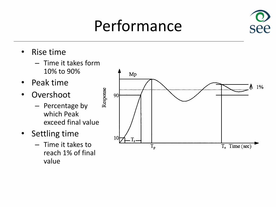
Performance

• Rise time– Time it takes form

10% to 90%

• Peak time

• Overshoot– Percentage by

which Peak exceed final value

• Settling time– Time it takes to

reach 1% of final value

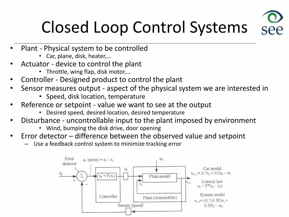
Closed Loop Control Systems• Plant - Physical system to be controlled

• Car, plane, disk, heater,…

• Actuator - device to control the plant• Throttle, wing flap, disk motor,…

• Controller - Designed product to control the plant• Sensor measures output - aspect of the physical system we are interested in

• Speed, disk location, temperature• Reference or setpoint - value we want to see at the output

• Desired speed, desired location, desired temperature

• Disturbance - uncontrollable input to the plant imposed by environment• Wind, bumping the disk drive, door opening

• Error detector – difference between the observed value and setpoint– Use a feedback control system to minimize tracking error

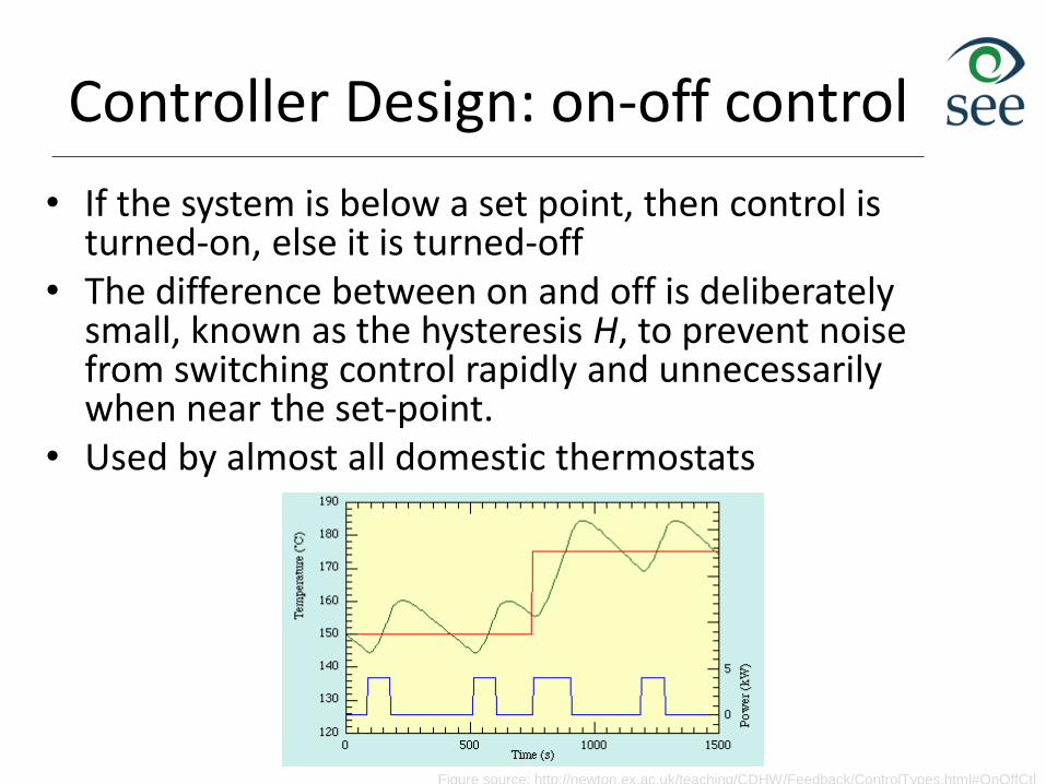
Controller Design: on-off control

• If the system is below a set point, then control is turned-on, else it is turned-off

• The difference between on and off is deliberately small, known as the hysteresis H, to prevent noise from switching control rapidly and unnecessarily when near the set-point.

• Used by almost all domestic thermostats

Figure source: http://newton.ex.ac.uk/teaching/CDHW/Feedback/ControlTypes.html#OnOffCtl

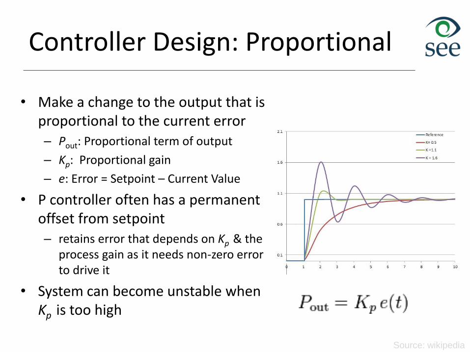
Controller Design: Proportional

• Make a change to the output that is proportional to the current error – Pout: Proportional term of output

– Kp: Proportional gain

– e: Error = Setpoint – Current Value

• P controller often has a permanent offset from setpoint– retains error that depends on Kp & the

process gain as it needs non-zero error to drive it

• System can become unstable when Kp is too high

Source: wikipedia

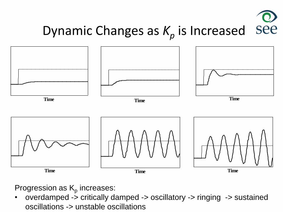
Dynamic Changes as Kp is Increased

Time Time Time

Time Time Time

Progression as Kp increases:

• overdamped -> critically damped -> oscillatory -> ringing -> sustained

oscillations -> unstable oscillations

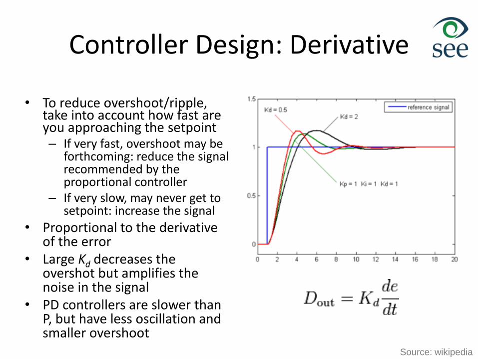
Controller Design: Derivative

• To reduce overshoot/ripple, take into account how fast are you approaching the setpoint– If very fast, overshoot may be

forthcoming: reduce the signal recommended by the proportional controller

– If very slow, may never get to setpoint: increase the signal

• Proportional to the derivative of the error

• Large Kd decreases the overshot but amplifies the noise in the signal

• PD controllers are slower than P, but have less oscillation and smaller overshoot

Source: wikipedia

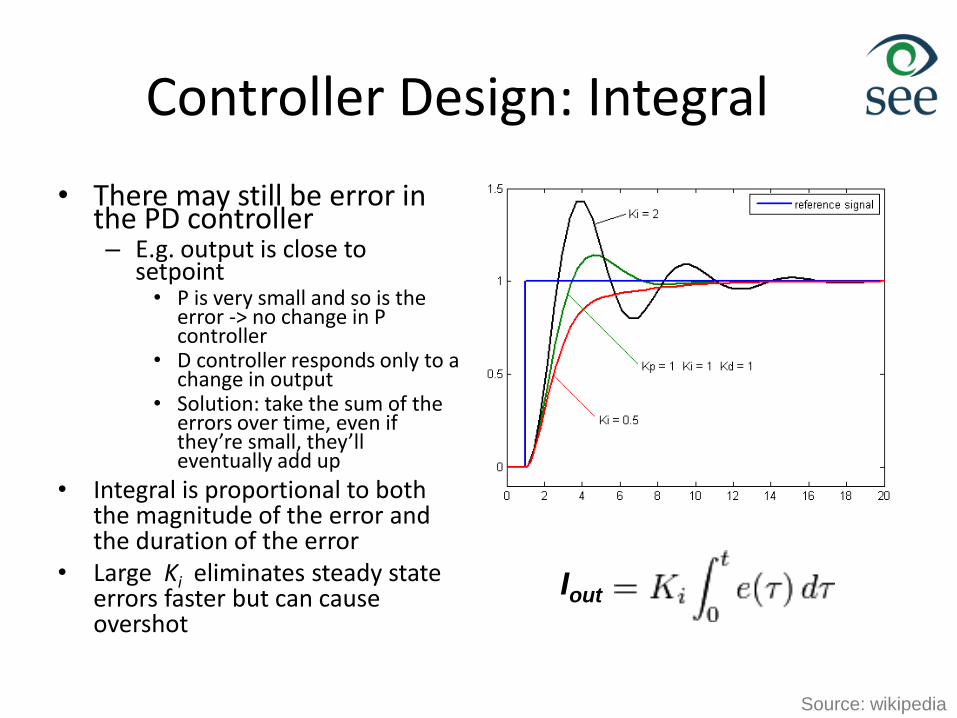
Controller Design: Integral

• There may still be error in the PD controller– E.g. output is close to

setpoint• P is very small and so is the

error -> no change in P controller

• D controller responds only to a change in output

• Solution: take the sum of the errors over time, even if they’re small, they’ll eventually add up

• Integral is proportional to both the magnitude of the error and the duration of the error

• Large Ki eliminates steady state errors faster but can cause overshot

Iout

Source: wikipedia

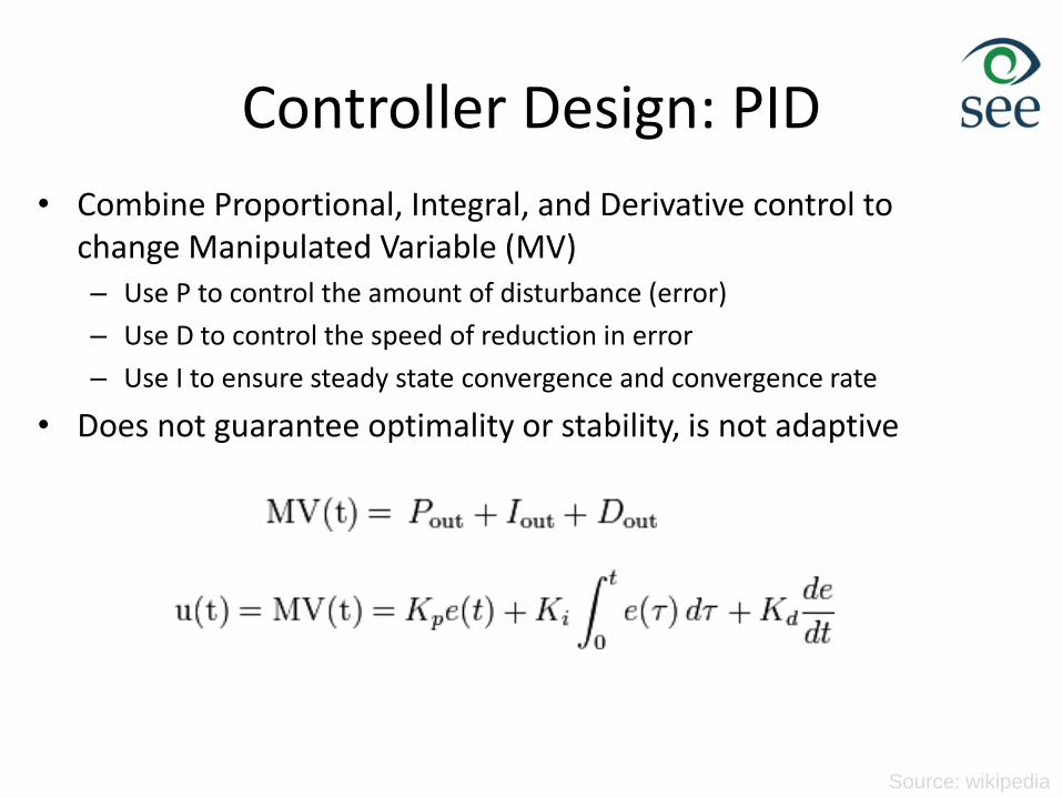
Controller Design: PID

• Combine Proportional, Integral, and Derivative control to change Manipulated Variable (MV)– Use P to control the amount of disturbance (error)

– Use D to control the speed of reduction in error

– Use I to ensure steady state convergence and convergence rate

• Does not guarantee optimality or stability, is not adaptive

Source: wikipedia

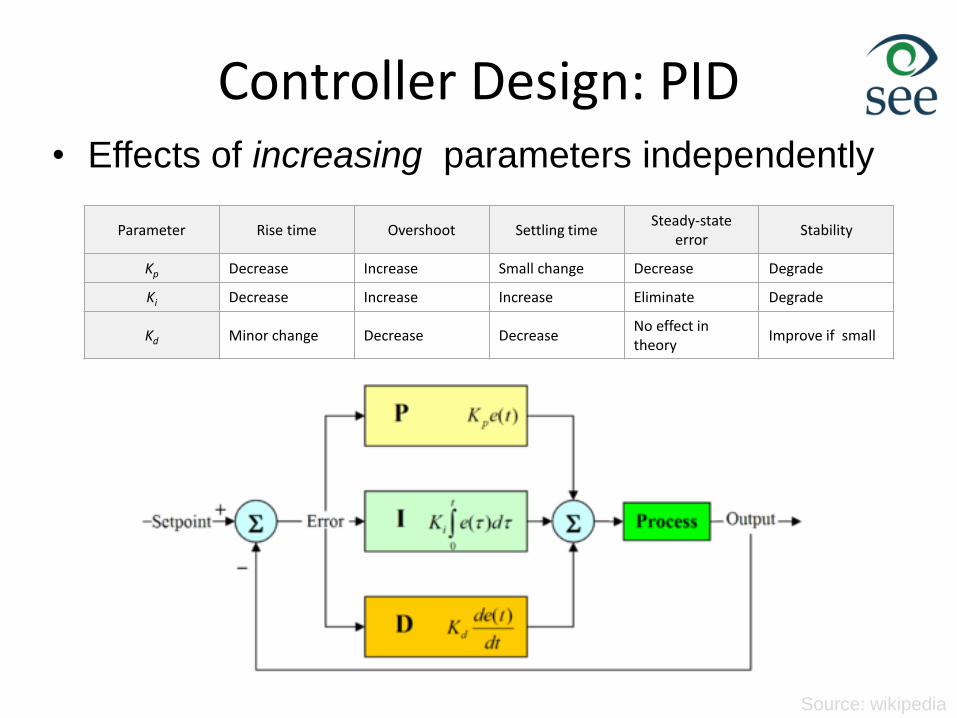
Controller Design: PID

Parameter Rise time Overshoot Settling timeSteady-state

errorStability

Kp Decrease Increase Small change Decrease Degrade

Ki Decrease Increase Increase Eliminate Degrade

Kd Minor change Decrease DecreaseNo effect in theory

Improve if small

• Effects of increasing parameters independently

Source: wikipedia

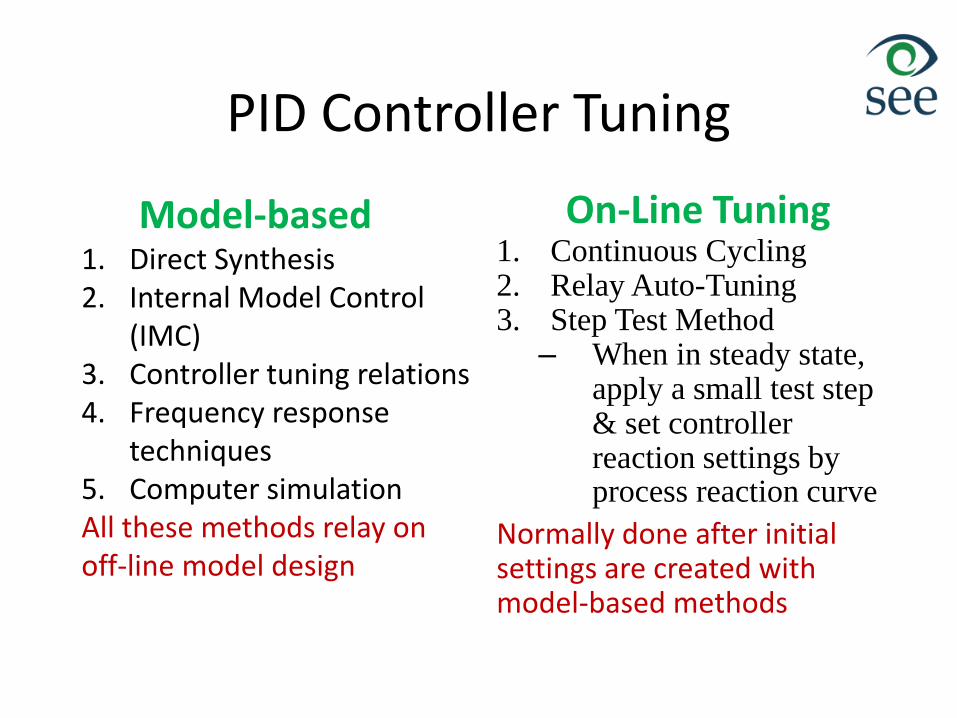
PID Controller Tuning

Model-based1. Direct Synthesis2. Internal Model Control

(IMC)3. Controller tuning relations4. Frequency response

techniques5. Computer simulationAll these methods relay on off-line model design

On-Line Tuning1. Continuous Cycling2. Relay Auto-Tuning3. Step Test Method

– When in steady state, apply a small test step & set controller reaction settings by process reaction curve

Normally done after initial settings are created with model-based methods

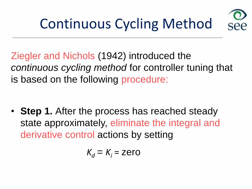
Continuous Cycling Method

Ziegler and Nichols (1942) introduced the

continuous cycling method for controller tuning that

is based on the following procedure:

• Step 1. After the process has reached steady

state approximately, eliminate the integral and

derivative control actions by setting

Kd = Ki = zero

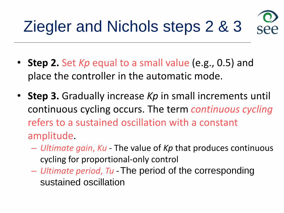
Ziegler and Nichols steps 2 & 3

• Step 2. Set Kp equal to a small value (e.g., 0.5) and place the controller in the automatic mode.

• Step 3. Gradually increase Kp in small increments until continuous cycling occurs. The term continuous cyclingrefers to a sustained oscillation with a constant amplitude. – Ultimate gain, Ku - The value of Kp that produces continuous

cycling for proportional-only control– Ultimate period, Tu - The period of the corresponding

sustained oscillation

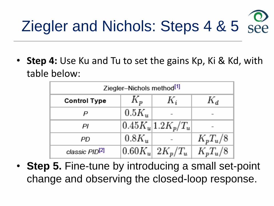
Ziegler and Nichols: Steps 4 & 5

• Step 4: Use Ku and Tu to set the gains Kp, Ki & Kd, with table below:

• Step 5. Fine-tune by introducing a small set-point

change and observing the closed-loop response.

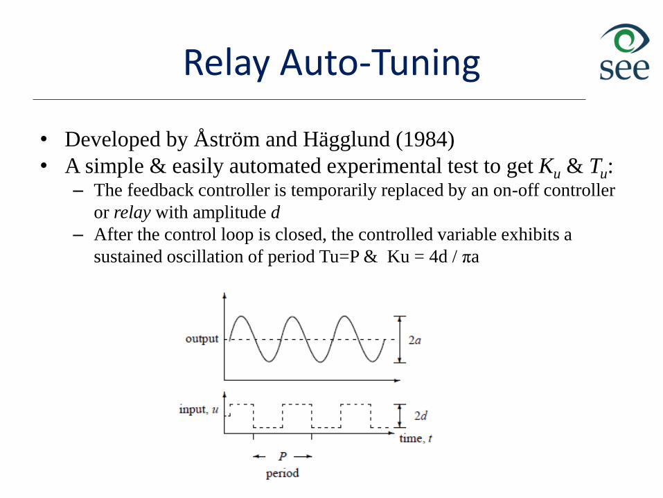
Relay Auto-Tuning

• Developed by Åström and Hägglund (1984)

• A simple & easily automated experimental test to get Ku & Tu: – The feedback controller is temporarily replaced by an on-off controller

or relay with amplitude d

– After the control loop is closed, the controlled variable exhibits a

sustained oscillation of period Tu=P & Ku = 4d / πa

Sources

• Peter Marwedel, “Embedded Systems Design,” 2004.

• Real-time DSP Lab, Prof. Brian Evans, UTA

• Ryerson Communications Lab, X. Fernando

• Daniel Mosse & David Willson

• Charles Williams; http://newton.ex.ac.uk/teaching/CDHW/Feedback/