Contemporary Engineering Sciences, Vol. 10, 2017, no. 9, 423 - 438

HIKARI Ltd, www.m-hikari.com https://doi.org/10.12988/ces.2017.612191

CPU and GPU Behaviour Modelling Versus

Sequential and Parallel Bias Field Correction

Fuzzy C-means Algorithm Implementations

Bouchaib Cherradi

STICE team, CRMEF-El Jadida, Morocco

LaROSERI laboratory, Chouaib Doukkali University, FS-El Jadida, Morocco

SSDIA laboratory, Hassan II University, ENSET-Mohammedia, Morocco

Noureddine Ait Ali

SSDIA laboratory, ENSET-Mohammedia, Hassan II University, Morocco

Ahmed El Abbassi

EPIM laboratory, My Ismail University, FST-Errachidia, Morocco

Omar Bouattane and Mohamed Youssfi

SSDIA laboratory, ENSET-Mohammedia, Hassan II University, Morocco

Copyright © 2017 Bouchaib Cherradi et al. This article is distributed under the Creative

Commons Attribution License, which permits unrestricted use, distribution, and reproduction in

any medium, provided the original work is properly cited.

Abstract

The correction of images corrupted by bias field artefact is still challenging

task both at accuracy level as on the computational plane. The work in this paper

focus on the second constraint by giving mathematical models of experimental

execution time per iteration ETPI(s) on GPU and CPU implementations and

speed-ups GPU/CPU(x) of the iterative Bias Field Correction Fuzzy C-means

clustering Algorithm (Both sequential BCFCM and parallel PBCFCM versions)

against the variable cluster number. In this study we characterize the behaviour of

these devices against the proposed implementations to show the optimal situation

that offers the best performance. The modelling results of cluster number variation

show interesting behaviours and are in good accordance to experimental ones.

424 Bouchaib Cherradi et al.

Keywords: BCFCM, image segmentation, parallel computing, GPU

1 Introduction

Image segmentation is fundamental step for computer vision, pattern

recognition, and medical image processing [1]. The main objective of image

segmentation is to divide an image automatically or semi-automatically into

non-overlapping regions, in such a way each region is homogeneous with respect

to some characteristics such as intensity or texture [2]. MRI image segmentation

has been studied for decades and many efforts have been devoted in the literature

to propose effective segmentation methods [3]. However, the existence of image

artifacts, such as intensity inhomogeneity, noise and partial volume in magnetic

resonance images (MRIs), affect the quantitative image analysis. The authors in [4]

reviewed, summarized and categorized the commonly used MRI images

segmentation algorithms with an emphasis on their characteristics, advantages and

disadvantages of these techniques.

A bias field is an artefact that is presented in the form of a low frequency signal

that corrupts MRI images because of the inhomogeneities in the magnetic fields of

the MRI machine. In the literature, there are two approaches to deal with bias field

artefact. The first approach can be used as a pre-processing step where the

corrupted MRI image is restored by dividing it by an estimated bias field signal

using a surface fitting approach [5]. The second approach shows how to modify an

algorithm such as the fuzzy c-means clustering algorithm [6] so that it can be used

to correct and segment an MRI image corrupted by a bias field signal [7]. The

correction of images corrupted by bias field artefact is still challenging task both

at accuracy level as on the computational plane [8].

Graphic processing units (GPUs) that were originally created for rendering

graphics, has emerged in the last decade as co-processing units for Central

Processing Units (CPU) and has become popular for General Purpose Graphical

Processing Units (GP-GPU) used for high performance computing, to accelerate

various digital signal processing applications, including medical image processing

[9-12].

Among the images segmentation algorithms dealing with intensity

in-homogeneities correction on GPU architecture, authors in [13] proposed an

extended mask-based version of the level set method with bias field, recently

proposed by Li et al. [14]. They propose CUDA implementations for the original

full domain and the extended mask-based versions, and compare the methods in

terms of speed, efficiency, and performance.

In our earlier work [15, 16], aiming a contribution to enhance the execution

time, we have proposed a parallel implementation of bias field correction fuzzy

CPU and GPU behaviour modelling versus sequential and… 425

c-means [7] on GPU architecture, this algorithm was experimented on three

different GPU devices. We have reached a speedup of 52x on GTX 580, 21x on

GTX 760 and 12x on GT 740 for image of size about 7 Megapixels on windows

32-bits platform. In the same context, the authors in [17] have proposed massively

parallel version of spatial fuzzy c-means SFCM clustering algorithm [18] that is a

modified version of Fuzzy c-means that relies with noise artefact by including

neighbour spatial function in the process of membership matrix updating. In

addition they proposed mathematical models for the evolution of execution time

related to one iteration and speed up of the GPU version compared to the CPU

version [19].

In this paper, our contribution is mainly focused to study and model the

behaviour of the used devices CPU and GPU against our both implementations

parallel (PBCFCM) and sequential (BCFCM) with respect to an important

variable that is the number of cluster that we want extract from the image. fitting

of experimental results leads to interesting statistical models that will guide users

of this algorithms to the optimal situation that offer the best performances.

The rest of this paper is organized as follows. In Section 2, we gave a review of

GPU Computing and CUDA programming model (NVidia GPU). Section 3

presents a review of the sequential version entitled bias field correction fuzzy

c-means clustering algorithm BCFCM [7] and our parallel version PBCFM. In

section 4 we present and discus our findings and results. Section 5, concludes the

paper and gives some perspectives for this work.

2 GPU Computing and CUDA Programming Model

Single instruction, multiple data (SIMD) architecture is one of the frameworks

that are used to accomplish data-parallelism. In this architecture, multiple

processors execute the same instructions on different data. Graphical processing

Units (GPUs) use this type of architecture. Methods and algorithms for image

processing are ideal computational tasks in a SIMD framework.

The NVidia’s GPU architecture contains a great number of elementary

processors that are composed of a large number of cores called streaming

processors (SP) clustered into multiprocessor (MP) units. Each SP involves an

arithmetic logical unit holding up integer and floating point operations. To adapt

the GPUs to the processing, we need to write parallel functions called kernels with

Compute Unified Device Architecture CUDA SDK [17].

The following figure explains the Nvidia GPU architecture and the interactions

possibilities with CPU (Host).

426 Bouchaib Cherradi et al.

Fig.1: Nvidia GPU architecture.

NVidia developed CUDA (Compute Unified Development Architecture) that

is a C library extension to provide a programming interface for users of his GPU

devices. The main program is managed by the CPU (host) that is responsible for

starting the program and executing serial code, while delegating parallel execution

of compute-intensive tasks to the GPU device. To have a massively parallel

version of a given algorithm with CUDA programming, we need to define C

functions (kernels), which are executed in parallel by multiple GPU threads.

Fig. 2: Execution model of a CUDA program on Nvidia GPU: Hierarchy Grid, Blocks

and Thread.

CPU and GPU behaviour modelling versus sequential and… 427

The CUDA program execution model is based on the fact that all threads run

the same kernel concurrently, and each one is associated with a unique thread ID.

Threads are arranged into three-dimensional thread blocks. Threads belonging to

the same block cooperate by sharing data through a very interesting component

that is shared memory and by synchronizing their execution through extremely

fast barriers. In contrast, threads belonging to different blocks cannot perform

barrier synchronizations with each other. Figure 2 shows an execution model of a

CUDA program based on the hierarchy grids, blocks and threads.

3 Sequential and Parallel Bias Field Correction Fuzzy C-means

Algorithm

The standard Fuzzy c-means (FCM) algorithm [6] objective function used for

partitioning an image containing {x1,…,xN} pixels into C clusters is given by:

(1)

Where,

ui,k: The degree of membership of data xk to the cluster vi,

vi: The prototypes (or centroid) of the cluster i,

N: The total number of pixels in the image

p: A weighting exponent parameter on each fuzzy membership value, it

determines the amount of fuzziness of the resulting classification according to:

(2)

In most works in the literature, the observed MRI signal is modelled as a

product of the true signal generated by the underlying anatomy, and a spatially

varying factor called the gain field.

(3)

Where Xk and Yk are the true and observed intensities at the kth pixel,

respectively, Gk is the gain field at the kth voxel. The application of a logarithmic

transformation to the intensities allows the artefact to be modelled as an additive

bias field.

(4)

Where xk and yk are the true and observed log-transformed intensities at the

kth pixel, respectively, and βk is the bias field at the kth pixel.

Ahmed et al [7] proposed a modification to (1) by introducing a term that

allows the labelling of a pixel (Voxel) to be influenced by the labels of its

immediate neighbourhood. The modified objective function is given by:

2

1 1

ik

C

i

N

k

p

ik vxuJ

C

i

N

k

ikikik iNukuuU1 1

,0,1,1,0

kkk GXY

kkk xy

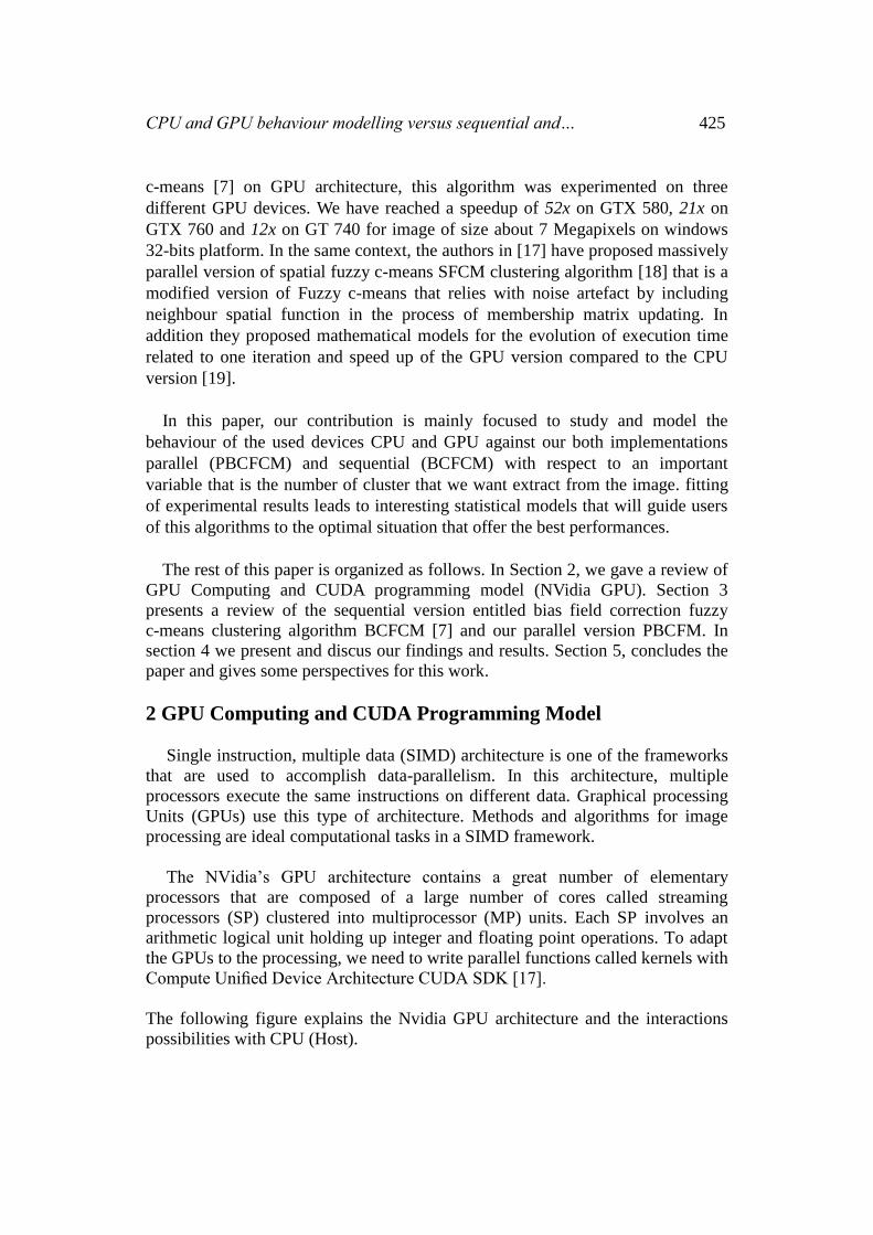
428 Bouchaib Cherradi et al.

(5)

Where:

Nk: Set of neighbour’s pixels that exist in a window around xk.

Nr: Cardinal of Nk.

α: Neighbours effect.

The new membership function is then given by:

(6)

Where:

(7)

And

(8)

The cluster prototype (centroid) updating is done by the expression:

(9)

The estimated bias field is given by the expression:

(10)

kr Ny

irr

C

i

N

k

p

ik

r

ikk

C

i

N

k

p

ikm vyuN

vyuJ2

1 1

2

1 1

C

j

p

j

r

jk

i

r

ik

ik

ND

ND

u

1

11

1

kr Ny

irri vy2

2

ikkik vyD

N

k

p

ik

N

k Ny

rr

r

kk

p

ik

i

u

yN

yu

Vkr

1

1

1

C

i

p

ik

C

i

i

p

ik

kk

u

vu

y

1

1

CPU and GPU behaviour modelling versus sequential and… 429

Algorithm 1 explains the main steps of this sequential algorithm.

Algorithm 1: Bias field Correction fuzzy C-Means Algorithm (BCFCM)

1: Set the parameters C, p, Nr, and α.

2. Choose the stopping criterion: Error,

3: Initialize the centroids vector V and estimated bias field.

4: repeat

5: Update the membership value U using Eq. (6)

6: Update the cluster centre vector V using Eq. (9)

7: Update the bias field estimated matrix β using Eq. (10)

8: until ErrorVV oldnew

We have implemented this sequential version on massively parallel

architecture that is a graphical processing unit, widely used actually in GPGPU.

The following flowchart shows the main stages of this algorithm implementation.

Fig. 3: PBCFCM flowchart.

For this algorithm we start with initializing the centroids vector and the

others parameters, then allocate and transfer data from CPU to GPU before the

loop iteration (stage 4 to stage 9 in figure 3). We have used two main CUDA

kernels, one to compute the membership matrix U by the expression (6) and the

430 Bouchaib Cherradi et al.

expressions needed for updating centroids in expression (9), the second to

compute the estimated bias field using the expression (10).

The loop starts (stage 4) by the call of the first kernel that computes both the

membership function and the expressions for updating centroids. In next stage, we

update the cluster centres vector in CPU with the expression (9) then we transfer

the new computed centroids vector to the GPU in order to compute the new

estimated bias field, and finally we verify the criterion termination based on final

cluster variation. In stage 9, if the stopping criterion is reached (algorithm

convergence) we show the results and exit; otherwise we loop to the stage 4. Note

that our strategy is based on the principle that the stages putting negligible

execution time are executed in Host (CPU). Only the 2 kernels execution time is

taken into consideration in our experiments, this is made by the CUDA instruction

cudaEventElapsedTime() used two times.

For the sequential version (BCFCM) implementation, the execution time is

observed only for portions of code equivalent to the 2 kernels to make a

significant comparison. The parallel implementation relies on the strategy

explained in the figure 4. This strategy consists on the execution of the potions

that consume time on GPU as CUDA kernels and the rest of the code is executed

on CPU that manages the global application code.

Fig. 4: Code Flow in GPU acceleration

The strengths of our parallel implementation for PBCFCM algorithm are:

(1) The exploitation of the shared memory for data to be clustered and

constant memory for centroids.

(2) The use of local thread registers and new functionalities of CUDA SDK.

This gave rise to more interesting results in terms of speed up as we will explain

in the following section.

CPU and GPU behaviour modelling versus sequential and… 431

4 Results and discussion

Before presenting the main results of this work, we present in the following tow

sub-sections, the hardware and software specifications in addition to the used

database for validation and experiments.

4.1 Software and Hardware specifications

Algorithm on CPU (sequential version) was implemented using Microsoft VC++

Toolkit and executed on Intel(R) Core(TM) i7-4770 8 cores 3.5GHz CPU to obtain

reference runtimes.

Parallelized portions of PBCFCM were implemented using CUDA SDK 6.5 and

executed on GTX 580 GPU device, execution times results were carried out to give

comparison.

In the following table we summarize the principal specifications of the used

devices.

TABLE 1: HARDWARE SPECIFICATIONS OF CPU AND GPU DEVICES, USED IN EXPERIMENTS

Device Property Value

CPU

Processor Intel Core i7-4770K

Clock speed 3.5 GHz

No. of Cores 4

No. of Threads… 8

RAM 16 GB

Operating system Windows 7, 64 bits

GPU

Chipset NVIDIA Geforce GTX 580

Processor clock 1544 Mhz (GF110)

Cuda cores 512

Total MP 16

Max Thread per Block 1024

Shared Memory 64 KB

Global Memory 1536 MB

Memory bus width 384 bits

Memory Bandwidth 192.4 GB/sec

Both sequential and parallel codes are compiled within Microsoft Visual Studio

2013 under Windows 7 (64-bit) operating system.

4.2 Images database

Since our main objective in this study is the evaluation and modelling of the

behaviour of the experimented material (CPU and GPU) against our

implementations parallel and sequential, we have chosen to build a database of

images from a test image often used as a reference in the field of digital image

processing that is Lena image.

To evaluate the behaviour of the GPU device when executing PBCFCM

algorithm against cluster number with different image sizes, we construct a bank of

432 Bouchaib Cherradi et al.

Lena images but with different densities that varies from 1024 pixels to about 10.2

million pixels (Mpixels).

Our experiments are done on the following images: 128x128 (img128), 512x512

(img512), 1024x1024 (img1024), 2048x2048 (img2048), 2708x2704 (img2708),

3000x3000 (img3000) and 3200x3200 (img3200).

The parameters set to validate and test the performances of our implementation

on segmentation of Lena image are as follow: 2<=C<=20, p=2, Nr=8 and α =0.85

(α represents the neighbors effect as mentioned in [7] for low-SNR images).

Note that the effectiveness and accuracy of the proposed PBCFCM algorithm has

been widely validated on T1-weighted and T2-weighted MRI images with different

densities and values of additional bias field.

4.3 Notations and definitions

In this paper, we will focus only on the number of cluster that we want to extract

from images (Cluster number), this variable is noted c.

In the goal to have magnitudes that can perfectly reflect the behaviour of the

experimented devices against the studied iterative clustering BCFCM and

PBCFCM algorithms, evaluate and compare the performances of the used devices

(CPU and GPU) against the execution of this algorithms, we define and consider

the following 2 magnitudes:

• The first one postpones the execution time reported to a single iteration, we

call it “Execution time per iteration in seconds” and we note it ETPI(s). This

magnitude will allow us to make an evaluation of the algorithms by

disregarding the number of iteration needed for convergence that depends on

the initial conditions and the size of the images. Indeed, the convergence of the

algorithm whatsoever for sequential or massively parallel implementation

depend of these variable.

• The second magnitude frequently used to evaluate the quality of a parallel

implementation of an image processing algorithms compared to its sequential

one is the ratio between the total execution time required for the convergence

on CPU and the total execution time needed for convergence on GPU taking

into account the same initial conditions. This ratio is called speed up

GPU/CPU(x) and noted SU(x).

4.4 Execution time per iteration behaviour modelling

In this subsection, we present some interesting results and finding relative to one

of the main ideas of this paper that is mathematically modelling of the variation of

the ETPI (s) magnitude, a function of the variation of cluster number for both

implementations (sequential and parallel). This will tell us about the behaviour of

the used devices overlooked this variable.

CPU and GPU behaviour modelling versus sequential and… 433

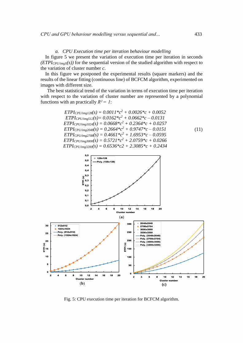
a. CPU Execution time per iteration behaviour modelling

In figure 5 we present the variation of execution time per iteration in seconds

(ETPICPU/imgX(s)) for the sequential version of the studied algorithm with respect to

the variation of cluster number c.

In this figure we postponed the experimental results (square markers) and the

results of the linear fitting (continuous line) of BCFCM algorithm, experimented on

images with different size.

The best statistical trend of the variation in terms of execution time per iteration

with respect to the variation of cluster number are represented by a polynomial

functions with an practically R² = 1:

ETPICPU/img128(s) = 0.0011*c2 + 0.0026*c + 0.0052

ETPICPU/img512(s)= 0.0162*c2 + 0.0662*c – 0.0131

ETPICPU/img1024(s) = 0.0668*c2 + 0.2364*c + 0.0257

ETPICPU/img2048(s) = 0.2664*c2 + 0.9747*c – 0.0151

ETPICPU/img2708(s) = 0.4661*c2 + 1.6953*c – 0.0595

ETPICPU/img3000(s) = 0.5721*c2 + 2.0759*c + 0.0266

ETPICPU/img3200(s) = 0.6536*c2 + 2.3085*c + 0.2434

(11)

(a)

(b) (c)

Fig. 5: CPU execution time per iteration for BCFCM algorithm.

434 Bouchaib Cherradi et al.

All these functions are polynomials of second order, which shows that the

increase in execution time reported to a single iteration follows a growing law and

this growth is even more pronounced as the number of cluster is more important.

These statistical models are in good concordance with the experimental results

and are only limited by the computational characteristics of the CPU and the

amount of memory in our setup.

b. GPU Execution time per iteration behaviour modelling

In this subsection, we intend to give from experimental executions of PBCFCM

algorithm on GTX580 device, mathematical models that reflect as closely as

possible the behaviour of this circuit when the number of clusters c that we want to

extract from the image varies, keeping constant the variable size of the image.

As in the previous subsection, we present in figure 6 the experimental results

(square markers) and the results of the fitting (continuous line) for PBCFCM

algorithm on GTX580 with 7 test images.

(a)

(b)

(c)

Fig. 6: GPU execution time per iteration for PBCFCM algorithm.

In the following, we will present the results relative to mathematically modelling of

the variation of the ETPI (s) a function of cluster number c. This will tell us about

CPU and GPU behaviour modelling versus sequential and… 435

the behaviour of the used GPU device overlooked the variation of the cluster

number c when executing PBCFCM with respect to the image data size parameter.

The best statistical trend of the variation in terms of execution time per iteration

with respect to the variation of cluster number c is represented also by a polynomial

functions with an practically R² = 1:

ETPIGTX580/img128(s) = 0.00002*c2 + 0.0002*c + 0.0006

ETPIGTX760/img512(s) = 0.0001*c2 + 0.0012*c + 0.0023

ETPIGTX760/img1024(s) = 0.0006*c2 + 0.0039*c + 0.0086

ETPIGTX760/img2048(s) = 0.0023*c2 + 0.015*c + 0.0303

ETPIGTX760/img2708(s) = 0.0042*c2 + 0.0221*c + 0.062

ETPIGTX760/img3000(s) = 0.0049*c2 + 0.0299*c + 0.0621

ETPIGTX760/img3200(s) = 0.0048*c2 + 0.0435*c + 0.0486

(12)

These models are in very good concordance with the experimental results and are

only limited by the computational characteristics of the GPU.

The limitation problem is observed at the test image img2708 for c=17, at the test

image img3000 for c=14 and at the test image img3200 for c=11. This is due to

insufficiency in terms of memory on the GPU device.

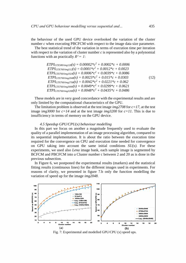
4.5 Speedup GPU/CPU(x) behaviour modelling

In this part we focus on another a magnitude frequently used to evaluate the

quality of a parallel implementation of an image processing algorithm, compared to

its sequential implementation. It is about the ratio between the execution time

required for the convergence on CPU and execution time needed for convergence

on GPU taking into account the same initial conditions SU(x). For these

experiments, we used also Lena image bank, each sample image is segmented by

BCFCM and PBCFCM into a Cluster number c between 2 and 20 as is done in the

previous subsection.

In Figure 6, we postponed the experimental results (markers) and the statistical

fitting results (continuous lines) for the different images used in experiments. For

reasons of clarity, we presented in figure 7.b only the function modelling the

variation of speed up for the image img2048.

(a)

(b)

Fig. 7: Experimental and modelled GPU/CPU (x) speed ups.

436 Bouchaib Cherradi et al.

Theoretical statistical fitting models show a perfect logarithmic behaviour of the

variation in speed-up versus cluster number c with an R² varying between 0.9668

and 0.9988.

img128

img512

img1024

img2048

img2708

img3000

img3200

SUGTX580/CPU(x) = 11.039ln(c) + 9.0877

SUGTX580/CPU(x) = 26.405ln(c) + 18.982

SUGTX580/CPU(x) = 26.046ln(c) + 26.30

SUGTX580/CPU(x) = 25.968ln(c) + 28.477

SUGTX580/CPU(x) = 26.028ln(c) + 29.597

SUGTX580/CPU(x) = 25.46ln(c) + 31.86

SUGTX580/CPU(x) = 26.877ln(c) + 29.692

(13)

All these functions present logarithmic behaviour, which shows that the increase

in speed up GPU/CPU (x) follows a growing law and this growth is even more

pronounced as the number of cluster is more important. This confirms that the use

of the parallel version of the algorithm is more desirable when the number of cluster

is greater to benefit from the computational capability of the GPU. But as is

mentioned in the previous section for the study on execution time per iteration

variable, the problem of limitation is observed from the test image img2708.

5 Conclusion

Bias field artefact correction is still a challenging problem in image processing

both at accuracy level as on the speed level; this is justified by the amount of recent

work in the literature on this subject. After proposing massively parallel algorithm

implementing one of the most popular technics (PCFCM) to correct and segment

images exploiting the performance offered by the modern Graphical Processing

Units (GPU), we are focused in this work on the characterization and modelling of

the behaviour of some devices against our implementations (parallel and

sequential) to provide information that could guide researchers and users of this

algorithms to the optimal situation that offer the best performances.

References

[1] Y. Wu, C. He, A convex variational level set model for image segmentation,

Signal Processing, 106 (2015), 123–133. https://doi.org/10.1016/j.sigpro.2014.07.013

[2] D.E. Ilea, P.F. Whelan, Image segmentation based on the integration of

colour-texture descriptors—a review, Pattern Recognition, 44 (2011), no. 10, 2479–2501. https://doi.org/10.1016/j.patcog.2011.03.005

[3] M.A. Balafar, A.R. Ramli, M.I. Saripan, S. Mashohor, Review of brain MRI

image segmentation methods, Artif. Intell. Rev., 33 (2010), no. 3, 261–274. https://doi.org/10.1007/s10462-010-9155-0

CPU and GPU behaviour modelling versus sequential and… 437

[4] Sepideh Yazdani, Rubiyah Yusof, Alireza Karimian, Mohsen Pashna &

Amirshahram Hematian, Image Segmentation Methods and Applications in

MRI Brain Images, IETE Technical Review, 32 (2015), no. 6, 413-427. https://doi.org/10.1080/02564602.2015.1027307

[5] M. Styner, C. Brechbuhler, G. Szckely, G. Gerig, Parametric estimate of

intensity inhomogeneities applied to MRI, IEEE Trans. on Medical Imaging, 19 (2000), no. 3, 153–165. https://doi.org/10.1109/42.845174

[6] J. C. Bezdek, R. Ehrlich, & W. Full, FCM: The fuzzy c-means clustering

algorithm, Computers & Geosciences, 10 (1984), no. 2-3, 191-203. https://doi.org/10.1016/0098-3004(84)90020-7

[7] M.N. Ahmed, N.A. Mohamed, A.A. Farag, T. Moriarty, A modified fuzzy

c-means algorithm for bias field estimation and segmentation of MRI data,

IEEE Trans. Med. Imaging, 21 (2002), 193–199.

https://doi.org/10.1109/42.996338

[8] Yin Kui-Ying, Sun Fa-Long, Zhou Sheng-Hua & Zhang Changchun, PAR

Model SAR Image Interpolation Algorithm on GPU with CUDA, IETE

Technical Review, 31 (2014), no. 4, 297-306.

https://doi.org/10.1080/02564602.2014.892736

[9] C. Feng, D. Zhao, M. Huang, Image segmentation using CUDA accelerated

non-local means denoising and bias correction embedded fuzzy c-means

(BCEFCM), Signal Processing, 122 (2016), 164–189.

https://doi.org/10.1016/j.sigpro.2015.12.007

[10] A. Eklund, P. Dufort, D. Forsberg, & S. M. LaConte, Medical image

processing on the GPU–Past, present and future, Medical Image Analysis, 17 (2013), no. 8, 1073-1094. https://doi.org/10.1016/j.media.2013.05.008

[11] G. Pratx, & L. Xing, GPU computing in medical physics: A review, Medical Physics, 38 (2011), no. 5, 2685-2697. https://doi.org/10.1118/1.3578605

[12] Erik Smistad, Thomas L Falch, Mohammadmehdi Bozorgi, Anne C Elster,

Frank Lindseth. Medical image segmentation on GPUs–A comprehensive

review, Medical Image Analysis, 20 (2015), no. 1, 1-18.

https://doi.org/10.1016/j.media.2014.10.012

[13] T. Ivanovska, R. Laqua, L. Wang, H. Volzke and K. Hegenscheid, Fast

Implementations of the Levelset Segmentation Method with Bias Field

Correction in MR Images: Full Domain and Mask-Based Versions, Chapter

in Pattern Recognition and Image Analysis, Vol. 7887, Springer Berlin:

Heidelberg, 2013, 674-681. https://doi.org/10.1007/978-3-642-38628-2_80

438 Bouchaib Cherradi et al.

[14] Chunming Li, Rui Huang, Zhaohua Ding, J C Gatenby, D N Metaxas, J C

Gore, A level set method for image segmentation in the presence of intensity

inhomogeneities with application to MRI, IEEE Transactions on Image Processing, 20 (2011), 2007–2016. https://doi.org/10.1109/tip.2011.2146190

[15] N. Aitali, B. Cherradi, A. El abbassi, O. Bouattane and M. Youssfi, Parallel

Implementation of Bias Field Correction Fuzzy C-Means Algorithm for

Image Segmentation, International Journal of Advanced Computer Science

and Applications (IJACSA), 7 (2016), no. 3, 367-374.

https://doi.org/10.14569/ijacsa.2016.070352

[16] N. Aitali, B. Cherradi, O. Bouattane, M. Youssfi, & A. Raihani, New

fine-grained clustering algorithm on GPU architecture for bias field

correction and MRI image segmentation, Procceding of the 27th IEEE

International Conference on Microelectronics (ICM2015), (2015), 118-121.

https://doi.org/10.1109/icm.2015.7438002

[17] N. Aitali, B. Cherradi, A. El Abbassi, O. Bouattane and M. Youssfi, GPU

based Implementation of Spatial Fuzzy C-means Algorithm for Image

Segmentation, 2016 4th IEEE International Conference on Information

Science and Technology (CiSt’16), (2016).

https://doi.org/10.1109/cist.2016.7805092

[18] Keh-Shih Chuang, Hong-Long Tzeng, Sharon Chen, Jay Wu, Tzong-Jer

Chen, Fuzzy c-means clustering with spatial information for image

segmentation. Computerized Medical Imaging and Graphics, 30 (2006), no.

1, 9-15. https://doi.org/10.1016/j.compmedimag.2005.10.001

[19] N. Aitali, B. Cherradi, A. El abbassi, O. Bouattane and M. Youssfi, Fuzzy

Spatial Clustering Algorithm on GPU: Characterization and Behavior

Modeling, 2nd Edition of the IEEE International Conference on Electrical

Sciences and Technologies in Maghreb (CISTEM’16), (2016).

[20] https://developer.nvidia.com/cuda-zone, 2015.

Received: December 31, 2016; Published: May 12, 2017