Embed Size (px)
Citation preview

1
CPSC 304 Introduction to Database Systems
Data Warehousing & OLAP
Textbook Reference Database Management Systems Sect. 25.1-25.5, 25.7-25.10
Other References: Database Systems: The Complete Book, 2nd edition
The Data Warehouse Toolkit, 3rd edition, by Kimball & Ross
Hassan Khosravi Based on slides from Ed, George, Laks, Jennifer Widom (Stanford),
and Jiawei Han (Illinois)

2
Learning Goals v Compare and contrast OLAP and OLTP processing (e.g., focus,
clients, amount of data, abstraction levels, concurrency, and accuracy).
v Explain the ETL tasks (i.e., extract, transform, load) for data warehouses.
v Explain the differences between a star schema design and a snowflake design for a data warehouse, including potential tradeoffs in performance.
v Argue for the value of a data cube in terms of: the type of data in the cube (numeric, categorical, counts, sums) and the goals of OLAP (e.g., summarization, abstractions).
v Estimate the complexity of a data cube in terms of the number of views that a given fact table and set of dimensions could generate, and provide some ways of managing this complexity.
3
Learning Goals (cont.) v Given a multidimensional cube, write regular SQL queries that
perform roll-up, drill-down, slicing, dicing, and pivoting operations on the cube.
v Use the SQL:1999 standards for aggregation (e.g., GROUP BY CUBE) to efficiently generate the results for multiple views.
v Explain why having materialized views is important for a data warehouse.
v Determine which set of views are most beneficial to materialize.
v Given an OLAP query and a set of materialized views, determine which views could be used to answer the query more efficiently than the fact table (base view).
v Define and contrast the various methods and policies for materialized view maintenance.

4
What We Have Focused on So Far ❖ OLTP (On-Line Transaction Processing)
– class of information systems that facilitate and manage transaction-oriented applications, typically for data entry and retrieval transaction processing.
– the system responds immediately to user requests.
– high throughput and insert- or update-intensive database management. These applications are used concurrently by hundreds of users.
❖ The key goals of OLTP applications are availability, speed, concurrency and recoverability.
source: Wikipedia

5
On-Line Transaction Processing v OLTP Systems are
used to “run” a business.
❖ Examples: Answering
queries from a Web interface, sales at cash registers, selling airline tickets, transactions at an ATM.
OLTP
Typical User Basically Everyone (Many Concurrent Users)
Type of Data Current, Operational, Frequent Updates
Type of Query Short, Often Predictable
# of Queries Many concurrent queries
Access Many reads, writes and updates
DB Design Application oriented
Schema E-R model
Normal Form Often 3NF
Typical Size MB to GB
Protection Concurrency Control, Crash Recovery
Function Day to day operations

6
Can We Do More?
❖ Increasingly, organizations are analyzing current and historical data to identify useful patterns and support business strategies. – “Decision Support”, “Business Intelligence”
❖ The emphasis is on complex, interactive, exploratory analysis of very large datasets created by integrating data from across all parts of an enterprise.

7
A Producer Wants to Know …
Who are our lowest/highest margin
customers ?
Who are my customers, and what products are they buying?
Which customers are most likely to go to the competition ?
What impact will new products/services
have on revenue and margins?
What product promo- -tions have the biggest
impact on revenue?
What is the most effective distribution
channel?

8
Data, Data, Everywhere, yet ... ❖ I can’t find the data I need
– Data is scattered over the network – Many versions, many sources, subtle
differences, incompatible formats, missing values
❖ I can’t get the data I need – Need an expert to get the data from
various sources ❖ I can’t understand the data I found
– Poorly documented ❖ I can’t use the data I found
– Results are unexpected – Not sure what I’m looking for – Data needs to be transformed

9
What is Data Warehouse? ❖ “A data warehouse is a subject-
oriented, integrated, time-variant,
and nonvolatile collection of data
in support of management’s
decision-making process.”
—W. H. Inmon
Recognized by many as the father of the data warehouse

10
Data Warehouse—Subject-Oriented
❖ Subject-Oriented: Data that gives information about a particular subject area such as customer, product, and sales instead of about a company's ongoing operations. 1. Focusing on the modeling and analysis of data for
decision makers, not on daily operations or transaction processing
2. Provides a simple and concise view around particular
subject issues by excluding data that are not useful in the decision support process

11
Application-Oriented
Members ID Name Level StartDate
111 Joe A 01/01/2008
222 Sue B 01/01/2008
333 Pat A 01/01/2008
ID Type Fee
A Gold $100
B Basic $50
Membership levels Visit Level ID Type Fee
YP Pool $15
NP No pool $10
Non-member Visits ID VID VisitDate
1 YP 01/01/2008
2 YP 01/01/2008
3 NP 01/01/2008
….
Subject-Oriented Revenue
R-ID Date By Amount
….
7235 01/01/2008 Non-Member $15
7236 01/01/2008 Member $100
7237 01/01/2008 Member $50
7238 01/01/2008 Member $100
7239 01/01/2008 Non-Member $10
7240 01/01/2008 Non-Member $15
…

12
Data Warehouse—Integrated
❖ Constructed by integrating multiple, heterogeneous data sources. – relational databases, XML, flat files, on-line transaction
records
❖ Data cleaning and data integration techniques are applied. – Ensure consistency in naming conventions, encoding
structures, attribute measures, etc. among different data sources. ◆ e.g., Hotel price depends on: currency, various room taxes,
whether breakfast or Internet is included, etc.
– When data from different sources is moved to the warehouse, it is cleaned and converted into a common format.

13
Extract, Transform, and Load (ETL) ❖ ETL refers to the processes used to:
– Extract data from homogeneous or heterogeneous data sources ◆ Common data-source formats include relational
databases, XML, Excel, and flat files.
– Transform the data and store it in a common, standardized format or structure, suitable for querying and analysis. ◆ An important function of transformation is data cleaning.
This operation may take 80% or more of the effort!
– Load the data into the data warehouse

14
A Typical Data Integration Scenario Part 1 of 2
❖ Consider Canada Safeway’s data sources: – Operational data from daily purchase transactions, in each store – Data about item placement on shelves – Supplier data – Data about employees, their compensation, etc. – Sales/promotion plans – Product categories and sub-categories; brands, types; customer
demographics; time and date of sale
❖ Each of the above is essentially an autonomous OLTP database (or set of tables) – Local queries; no queries cutting across multiple databases – Data must be current at all times – Support for concurrency, recovery, and transaction management are a
must.

15
A Typical Data Integration Scenario, Part 2 of 2
❖ Consider the following use-case queries:
❖ How does the sale of hamburgers for Feb. 2015 compare with that for Feb. 2014?
❖ What were the sales of ketchup like last week (when hamburgers and ketchup were placed next to each other) compared to the previous week (when they were far apart)?
❖ What was the effect of the promotion on ground beef on the sales of hamburger buns and condiments?
❖ How has the reorganization of the store(s) impacted sales? ❖ Be specific here to try to see cause-and-effect—especially
with respect to prior periods’ sales. ❖ What was the total sales volume on all frozen food items (not
just one item or a small set of items)?

16
Data Warehouse Integration Challenges
❖ When getting data from multiple sources, we must eliminate mismatches (e.g., different currencies, units/scales, schemas)
❖ e.g., Shell Canada (Calgary), Shell Oil (Houston), Royal Dutch Shell (Netherlands), etc. may need to deal with data mismatches throughout the multinational organization: – Exercise: Provide some examples of mismatches that
might occur in this example. Here are a few to start: ◆ Different countries have different currencies (USD, CAD, EUR,
etc.), so how should we handle this? – What exchange rate should we use?
◆ Gallons vs. litres vs. barrels ◆ Different grades of crude oil ◆ Add some examples of your own

17
DW Integration Challenges (cont.)
❖ e.g., Shell may need to deal with data mismatches throughout the multinational organization: – Multiple cu rrencies and dynamic exchange rates – Gallons vs. litres; thousands of cubic feet (of gas) vs. cubic
metres vs. British Thermal Units (BTUs) – Different suppliers, contractors, unions, and business
partner relationships – Different legal, tax, and royalty structures – Local, provincial, federal, and international regulations – Different statutory holidays (when reporting holiday sales) – Light Sweet Crude (Nigeria) vs. Western Canada Select
(Alberta, heavier crude oil) – Joint ownership of resources (partners) – Retail promotions in its stores; different products

18
DW—Time Variant
❖ Time-Variant: All data in the data warehouse is associated with a particular time period.
❖ The time horizon for a DW is significantly longer than for operational systems.
– Operational DB: all data is current, and subject to change
– DW: contains lots of historical data that may never change, but may have utility to the business when determining trends, outliers, profitability; effect of business decisions or changes to policy; pre-compute aggregations; record monthly balances or inventory; etc. ◆ DW data is tagged with date and time, explicitly or implicitly

19
DW—Non-volatile
❖ Non-volatile: Data is stable in a data warehouse. More data is added, but data is not removed. This enables management to gain a consistent picture of the business.
❖ Real-time updates of operational data typically does not
occur in the DW environment, but can be done in bulk later (e.g., overnight, weekly, monthly).
– DW does not require transaction processing, recovery,
and concurrency control mechanisms.
– DW focuses on two major operations:
◆ loading of data and accessing of data

20
Operational DBMS vs. Data Warehouse ❖ Operational DBMS
– Day-to-day operations: purchasing, inventory, banking, payroll, manufacturing, registration, accounting, etc.
– Used to run a business
❖ Data Warehouse – Data analysis and
decision making – Integrated data spanning
long time periods, often augmented with summary information
– helps to “optimize” the business

21
Why a Separate Data Warehouse? ❖ High performance for both systems
– DBMS— tuned for OLTP: access methods, indexing, concurrency control, recovery
– Warehouse—tuned for complex queries, multidimensional views, consolidation
❖ Different types of queries – Extensive use of statistical functions which are poorly
supported in DBMS
– Running queries that involve conditions over time or aggregations over a time period, which are poorly supported in a DBMS
– Running related queries that are generally written as a collection of independent queries in a DBMS

22
On-Line Analytical Processing
❖ Technology used to perform complex analysis of the data in a data warehouse. – OLAP is a category of software technology that enables
analysts, managers, and executives to gain insight into data through fast, consistent, interactive access to a wide variety of possible views of information.
– The data has been transformed from raw data to reflect the dimensionality of the enterprise as understood by the user.
❖ OLAP queries are, typically: – Full of grouping and aggregation – Few, but complex queries -- may run for hours

23
OLTP vs. OLAP OLTP OLAP
Typical User Basically Everyone (Many Concurrent Users)
Managers, Decision Support Staff (Few)
Type of Data Current, Operational, Frequent Updates
Historical, Mostly read-only
Type of Query Short, Often Predictable Long, Complex
# query Many concurrent queries Few queries
Access Many reads, writes and updates Mostly reads
DB design Application oriented Subject oriented
Schema E-R model, RDBMS Star or snowflake schema
Normal Form Often 3NF Unnormalized
Typical Size MB to GB GB to TB
Protection Concurrency Control, Crash Recovery
Not really needed
Function Day to day operation Decision support

24
Actionable Business Intelligence ❖ Business Intelligence involves analyzing data and
making actionable decisions based on that information, such as: – Deciding what products to stock – Deciding what products to put on sale, or what promotions
to offer – Deciding which product lines to focus on, or discontinue – If several items are frequently purchased together, or within
a close period of time, consider putting one of them on special, so that even if someone wasn’t planning on buying them, the person is now tempted to do so. ◆ e.g., hamburger and ketchup – usually co-purchased; put one on sale
and examine effect on the other

25
❖ Business Intelligence involves analyzing data and making actionable decisions based on that information, such as: – Estimating the lift provided by a promotion, that is,
comparing the total sales of related products and services during a period of time vs. the total sales normally. ◆ e.g., Suppose Honda Civics go on sale for $3000 off in late
Fall, and more people wind up buying them because of that promotion.
◆ But, if the sales for regularly-priced Honda Accords go down during the same period, or if Christmas sales of Honda Civics go down, there may be no lift … or it may be negative.
Actionable Business Intelligence

26
❖ In essence, the goal of business intelligence is to make strategic business decisions that improve sales, profits, response times, customer satisfaction, customer relationships, etc.
Actionable Business Intelligence

27
Data Warehousing
❖ The process of constructing
and using data warehouses
is called data warehousing.
EXTERNAL DATA SOURCES
EXTRACT TRANSFORM LOAD REFRESH
DATA WAREHOUSE Metadata
Repository
SUPPORTS
OLAP DATA MINING

28
Business Intelligence: 3 Major Areas 1. Data Warehousing
– Consolidate and integrate operational OLTP databases from many sources into one large, well-organized repository ◆ e.g., acquire data from k different stores or branches ◆ Must handle conflicts in schemas, semantics, platforms, integrity
constraints, etc. ◆ May need to perform data cleaning
– Load data through periodic updates ◆ Synchronization and currency considerations
– Maintain an archive of potentially useful historical data including data that is an aggregation or summary, but has been pre-processed.
❖ Data Warehouses are then used to perform OLAP and Data Mining (DM).

29
Business Intelligence: 3 Major Areas 2. OLAP
– Perform complex SQL queries and views, including trend analysis, drilling down for more details, and rolling up to provide more easily understood summaries.
– Perform interactive, exploratory data analysis – Queries are based on spreadsheet-style operations, albeit
on a “multidimensional” scale/view of data. – Queries are normally performed by domain (business)
experts rather than database experts. 3. Data Mining
– Exploratory search for interesting trends (patterns) and anomalies (e.g., outliers, deviations) using more sophisticated algorithms (as opposed to queries).

30
That is all great, but what are the challenges with data warehousing?
❖ Semantic Integration: Extract, Transform, Load challenges. We already talked about the Shell example.
❖ Heterogeneous Sources: Must access data from a variety of source formats and repositories
– DB2, Oracle, SQL Server, Excel, Word, text-based files – Hundreds of COTS (commercial off-the-shelf software)
packages, with export facilities.
❖ Load, Refresh, and Purge Activities: Must load data, periodically refresh it, and purge old data
– How often?

31
Data Warehousing Challenges
❖ Metadata Management: Must keep track of source, load time, and other information for all data in the data warehouse.
❖ Answering Queries Quickly: Approximate answers are often OK. – Better to give an approximate answer quickly, than an
exact answer n minutes later – Sampling – Snapshot (if the data keeps changing or we want an
easily accessible point-in-time result (e.g., end-of-month sales figures)

32
Data Warehousing Challenges (Answering Queries Quickly)
❖ Pre-compute and store (materialize) some answers – Use a Data Cube to store summarized/aggregated data to
answer queries, instead of having to go through a much bigger table to find the same answer.
– The computation is similar in spirit to relational query optimization which is studied in detail in CPSC 404.
– Use disk-resident algorithms because there is simply too
much data to fit into memory all at once. – This trend is changing: industry is moving to memory-
resident OLAP.

33
OLAP Queries
❖ OLAP queries are full of groupings and aggregations.
❖ The natural way to think about such queries is in terms of a multidimensional model, which is an extension of the table model in regular relational databases.
❖ This model focuses on: – a set of numerical measures: quantities that are
important for business analysis, like sales, etc. – a set of dimensions: entities on which the measures
depend on, like location, date, etc.

34
Multidimensional Data Model ❖ The main relation, which relates dimensions to a
measure via foreign keys, is called the fact table. – Recall that a FK in one table refers to a candidate key (and most
of the time, the primary key) in another table. – The fact table has FKs to the dimension tables. – These mappings are essential.
❖ Each dimension can have additional attributes and an associated dimension table. – Attributes can be numeric, categorical, temporal, counts, sums
❖ Fact tables are much larger than dimensional tables. – Why?
❖ There can be multiple fact tables. – You may wish to have many measures in the same fact table.

35
Design Issues v The schema that is very common in OLAP
applications, is called a star schema: § one table for the fact, and § one table per dimension
v The fact table is in BCNF. v The dimension tables are not normalized. They are
small; updates/inserts/deletes are relatively less frequent. So, redundancy is less important than good query performance.

36
Running Example
Sales(storeID, itemID, custID, price)
Store(storeID, city, county, state)
Item(itemID, category, color)
Customer(custID, cname, gender, age)
storeID itemID custID price
storeID city county state
itemID category color
custID cname gender age
❖ Star Schema – fact table references dimension tables – Join → Filter → Group → Aggregate

37
Dimension Hierarchies
❖ For each dimension, the set of values can be organized in a hierarchy:
Customer Item Store
County
City Category
State
Color Gender Age

38
Running Example (cont.)
Customer Item
Store
County
City Category
State
Color Gender Age
Sales(storeID, itemID, custID, price)
Store(storeID, city, county, state)
Item(itemID, category, color)
Customer(custID, cname, gender, age)
M F
20 21 22 25 T-shirt
Jacket Red Blue
CA WA
Santa Clara Santa Mateo King
Palo Alto Mountain View Menlo Park Belmont Seattle Redmond

39
Full Star Join ❖ An example of how to find the full star join (or complete star
join) among 4 tables (i.e., fact table + all 3 of its dimensions) in a Star Schema: – Join on the foreign keys
❖ If we join fewer than all dimensions, then we have a star join. ❖ In general, OLAP queries can be answered by computing
some or all of the star join, then by filtering, and then by aggregating.
SELECT * FROM Sales F, Store S, Item I, Customer C WHERE F.storeID = S.storeID and F.itemID = I.itemID and F.custID = C.custID;

40
Full Star Join Summarized
SELECT storeID, itemID, custID, SUM(price) FROM Sales F GROUP BY storeID, itemID, custID;
Cus
tom
ers
65 10 Store1
Store2 Store3
Store5 Store4
Cust3
Cust2
Cust1
Item4 Item3 Item2 Item1 Items
❖ Find total sales by store, item, and customer.
storeID itemID custID Sum (price) store1 item1 cust1 10 store1 item3 cust2 65 … … … …

41
OLAP Queries – Roll-up ❖ Roll-up allows you to summarize data by:
– changing the level of granularity of a particular dimension
– dimension reduction

42
Roll-up Example 1 (Hierarchy) C
usto
mer
s
Store1 Store2
Store3
Store5 Store4
Cust3
Cust2
Cust1
Item4 Item3 Item2 Item1 Items
Cus
tom
ers Cust3
Cust2
Cust1
Item4 Item3 Item2 Item1 Items
King San Mateo
Santa Clara
SELECT county, itemID, custID, SUM(price) FROM Sales F, Store S WHERE F.storeID = S.storeID GROUP BY county, itemID, custID;
❖ Use Roll-up on total sales by store, item, and customer to find total sales by item and customer for each county.
SELECT storeID, itemID, custID, SUM(price) FROM Sales F GROUP BY storeID, itemID, custID;
43
Roll-up Example 2 (Hierarchy) ❖ Use Roll-up on total sales by item, customer,
and county to find total sales by item, gender and county.
Cus
tom
ers Cust3
Cust2
Cust1
Item4 Item3 Item2 Item1 Items
King San Mateo
Santa Clara
SELECT county, itemID, custID, SUM(price) FROM Sales F, Store S WHERE F.storeID = S.storeID GROUP BY county, itemID, custID;
Cus
otm
ers
female
male
Item4 Item3 Item2 Item1 Items
King San Mateo
Santa Clara
SELECT county, itemID, gender, SUM(price) FROM Sales F, Store S, Customer C WHERE F.storeID = S.storeID and F.custID = C.custID GROUP BY county, itemID, gender;

44
Roll-up Example 3 (Dimension) ❖ Use Roll-up on total sales by item, gender and
county to find total sales by item for each county.
Cus
tom
ers
female
male
Item4 Item3 Item2 Item1 Items
King San Mateo
Santa Clara
SELECT county, itemID, gender, SUM(price) FROM Sales F, Store S, Customer C WHERE F.storeID = S.storeID AND F.custID = C.custID GROUP BY county, itemID, gender;
Item4 Item3 Item2 Item1 Items
King San Mateo
Santa Clara SELECT county, itemID, SUM(price) FROM Sales F, Store S WHERE F.storeID = S.storeID GROUP BY county, itemID;

45
OLAP Queries – Drill-down ❖ Drill-down: reverse of roll-up
– From higher level summary to lower level summary (i.e., we want more detailed data)
– Introducing new dimensions
46
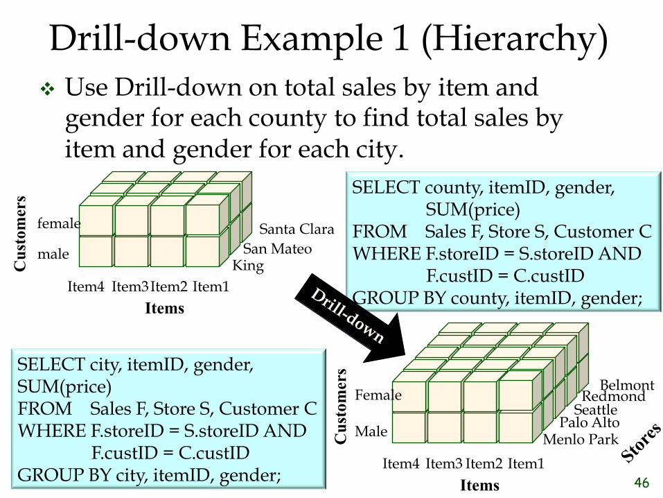
Drill-down Example 1 (Hierarchy) ❖ Use Drill-down on total sales by item and
gender for each county to find total sales by item and gender for each city.
Cus
tom
ers
female
male
Item4 Item3 Item2 Item1 Items
King San Mateo
Santa Clara
SELECT county, itemID, gender, SUM(price) FROM Sales F, Store S, Customer C WHERE F.storeID = S.storeID AND F.custID = C.custID GROUP BY county, itemID, gender;
SELECT city, itemID, gender, SUM(price) FROM Sales F, Store S, Customer C WHERE F.storeID = S.storeID AND F.custID = C.custID GROUP BY city, itemID, gender;
Cus
tom
ers
Menlo Park Palo Alto
Seattle
Belmont Redmond Female
Male
Item4 Item3 Item2 Item1 Items

47
Drill-down Example 2 (Dimension) ❖ Use Drill-down on total sales by item and
county to find total sales by item and gender for each county.
Cus
tom
ers
female
male
Item4 Item3 Item2 Item1 Items
King San Mateo
Santa Clara
SELECT county, itemID, gender, SUM(price) FROM Sales F, Store S, Customer C WHERE F.storeID = S.storeID AND F.custID = C.custID GROUP BY county, itemID, gender;
Item4 Item3 Item2 Item1 Items
King San Mateo
Santa Clara SELECT county, itemID, SUM(price) FROM Sales F, Store S WHERE F.storeID = S.storeID GROUP BY county, itemID;
48
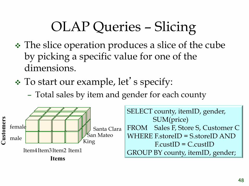
OLAP Queries – Slicing ❖ The slice operation produces a slice of the cube
by picking a specific value for one of the dimensions.
❖ To start our example, let’s specify: – Total sales by item and gender for each county
SELECT county, itemID, gender, SUM(price) FROM Sales F, Store S, Customer C WHERE F.storeID = S.storeID AND F.custID = C.custID GROUP BY county, itemID, gender;
Cus
tom
ers
female
male
Item4 Item3 Item2 Item1 Items
King San Mateo
Santa Clara

49
Slicing Example 1 ❖ Use Slicing on total sales by item and gender for each
county to find total sales by item and gender for Santa Clara.
SELECT county, itemID, gender, SUM(price) FROM Sales F, Store S, Customer C WHERE F.storeID = S.storeID AND F.custID = C.custID GROUP BY county, itemID, gender;
Cus
tom
ers
Female
Male
Item4 Item3 Item2 Item1 Items
Santa Clara
SELECT itemID, gender, SUM(price) FROM Sales F, Store S, Customer C WHERE F.storeID = S.storeID AND F.custID = C.custID AND S.county = 'Santa Clara' GROUP BY itemID, gender;
Cus
tom
ers
female
male
Item4 Item3 Item2 Item1 Items
King San Mateo
Santa Clara

50
Slicing Example 2 ❖ Use Slicing on total sales by item and gender for
each county to find total sales by gender and county for T-shirts.
SELECT county, itemID, gender, SUM(price) FROM Sales F, Store S, Customer C WHERE F.storeID = S.storeID AND F.custID = C.custID GROUP BY county, itemID, gender;
SELECT county, gender, SUM(price) FROM Sales F, Store S, Customer C, Item I WHERE F.storeID = S.storeID AND F.custID = C.custID AND F.itemID = I.itemID AND category = 'Tshirt' GROUP BY county, gender;
Cus
tom
ers
Female
Male
T-shirt Items
King San Mateo
Santa Clara
Cus
tom
ers
female
male
Item4 Item3 Item2 Item1 Items
King San Mateo
Santa Clara

51
OLAP Queries – Dicing ❖ The dice operation produces a sub-cube by
picking specific values for multiple dimensions.
❖ To start our example, let’s specify: – Total sales by gender, item, and city
SELECT city, itemID, gender, SUM(price) FROM Sales F, Store S, Customer C WHERE F.storeID = S.storeID AND F.custID = C.custID GROUP BY city, itemID, gender;
Cus
tom
ers
Menlo Park Palo Alto
Seattle
Belmont Redmond Female
Male
Item4 Item3 Item2 Item1 Items

52
Dicing Example 1 ❖ Use Dicing on total sales by gender, item, and
city to find total sales by gender, category, and city for red items in the state of California (CA).
Cus
tom
ers
Female
Male
T-shirt Jacket
Items
Menlo Park Palo Alto
Belmont
SELECT category, city, gender, SUM(price) FROM Sales F, Store S, Customer C, Item I WHERE F.storeID = S.storeID AND F.custID = C.custID AND F.itemID = I.itemID AND color = 'red' AND state = 'CA' GROUP BY category, city, gender;
SELECT city, itemID, gender, SUM(price) FROM Sales F, Store S, Customer C WHERE F.storeID = S.storeID AND F.custID = C.custID GROUP BY city, itemID, gender;
Cus
tom
ers
Menlo Park Palo Alto
Seattle
Belmont Redmond Female
Male
Item4 Item3 Item2 Item1 Items

53
Clicker Question ❖ Consider a fact table Sales(saleID, itemID, color, size, qty,
unitPrice), and the following three queries:
❖ Q1: SELECT itemID, color, size, Sum(qty*unitPrice) FROM Sales GROUP BY itemID, color, size
❖ Q2: SELECT itemID, size, Sum(qty*unitPrice) FROM Sales GROUP BY itemID, size
❖ Q3: SELECT itemID, size, Sum(qty*unitPrice) FROM Sales WHERE size < 10 GROUP BY itemID, size
❖ Which of the following statements is correct? A: Going from Q2 to Q3 is an example of roll-up. B: Going from Q2 to Q1 is an example of drill-down. C: Going from Q3 to Q2 is an example of roll-up. D: Going from Q1 to Q2 is an example of drill-down.

54
Clicker Question ❖ Consider a fact table Sales(saleID, itemID, color, size, qty,
unitPrice), and the following three queries:
❖ Q1: SELECT itemID, color, size, Sum(qty*unitPrice) FROM Sales GROUP BY itemID, color, size
❖ Q2: SELECT itemID, size, Sum(qty*unitPrice) FROM Sales GROUP BY itemID, size
❖ Q3: SELECT itemID, size, Sum(qty*unitPrice) FROM Sales WHERE size < 10 GROUP BY itemID, size
❖ Which of the following statements is correct? A: Going from Q2 to Q3 is an example of roll-up. B: Going from Q2 to Q1 is an example of drill-down. C: Going from Q3 to Q2 is an example of roll-up. D: Going from Q1 to Q2 is an example of drill-down.
Slicing Correct
Roll-up Filtering
55
OLAP Queries – Pivoting ❖ Pivoting is a visualization operation that allows
an analyst to rotate the cube in space in order to provide an alternative presentation of the data.

56
Pivoting Example 1 ❖ From total sales by store and customer pivot to
find total sales by item and store.
SELECT storeID, custID, sum(price) FROM Sales GROUP BY storeID, custID;
Store1 Store2
Store3
Store5 Store4
Cust3
Cust2
Cust1 Cus
tom
ers
Store1 Store2
Store3
Store5 Store4
Item4 Item3 Item2 Item1 Items
SELECT storeID, itemID, sum(price) FROM Sales GROUP BY storeID, itemID;

57
Aggregating over Multiple Fact Tables
Cus
tom
ers Cust3
Cust2
Cust1
Item4 Item3 Item2 Item1 Items
SELECT itemID, sum(price) FROM Sales GROUP BY itemID;
SELECT custID, sum(price) FROM Sales GROUP BY custID;
SELECT storeID, sum(price) FROM Sales GROUP BY storeID;
SELECT sum(price) FROM Sales
Store1 Store2
Store3
Store5 Store4
Cus
tom
ers
Store1 Store2
Store3
Store5 Store4
Cust3
Cust2
Cust1
Item4 Item3 Item2 Item1 Items

58
v A data cube is a k-dimensional object containing both fact data and dimensions.
v A cube contains pre-calculated, aggregated, summary information to yield fast queries.
Cus
tom
ers
Store1 Store2
Store3 Store5
Store4
Cust3
Cust2
Cust1
Item4 Item3 Item2 Item1 Items
Data Cube

59
Data Cube (cont.) ❖ The small, individual blocks in the multidimensional cube
are called cells, and each cell is uniquely identified by the members from each dimension.
❖ The cells contain a measure group, which consists of one or more numeric measures. These are facts (or aggregated facts). An example of a measure is the dollar value in sales for a particular product
Cus
tom
ers
Store1 Store2
Store3
Store5 Store4
Cust3
Cust2
Cust1
Item4 Item3 Item2 Item1 Items

60
The CUBE Operator ❖ Roll-up, Drill-down, Slicing, Dicing, and Pivoting
operations are expensive.
❖ SQL:1999 extended GROUP BY to support CUBE (and ROLLUP)
❖ GROUP BY CUBE provides efficient computation of
multiple granularity aggregates by sharing work (e.g., passes over fact table, previously computed aggregates)

61
Clicker Question
❖ If we have 2 stores, 5 items, and 10 customers, how many potential "entries" are there in the data cube? (The cube diagram is just an arbitrary example.)
❖ A: 17 ❖ B: 100 ❖ C: 117 ❖ D: 198 ❖ E: none of the above

62
Clicker Question
❖ If we have 2 stores, 5 items, and 10 customers, how many potential "entries" are there in the data cube? (The cube diagram is just an arbitrary example.)
❖ A: 17 ❖ B: 100 ❖ C: 117 ❖ D: 198 ❖ E: none of the above ❖ One way: 2*5*10 + 2*5 + 2*10 + 5*10 +2 + 5 + 10 +1 ❖ Another way: (2+1) * (5+1) * (10+1) = 3 * 6 * 11

63
Clicker Question ❖ How many standard SQL queries are required
for computing all of the cells of the cube?
❖ A: 2 ❖ B: 4 ❖ C: 6 ❖ D: 8 ❖ E: 10

64
Clicker Question ❖ How many standard SQL queries are required for
computing all of the cells of the cube?
A k-D cube can be represented as a series of (k-1)-D cubes. § The cube is exponential in the number of cells.
D: 8
{S, T, C}
{S, T} {S, C} {T, C}
{S} {T} {C}
{}
65
The CUBE Operator (cont.)
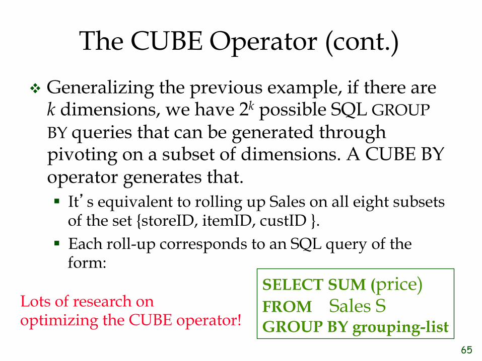
v Generalizing the previous example, if there are k dimensions, we have 2k possible SQL GROUP BY queries that can be generated through pivoting on a subset of dimensions. A CUBE BY operator generates that. § It’s equivalent to rolling up Sales on all eight subsets
of the set {storeID, itemID, custID }. § Each roll-up corresponds to an SQL query of the
form: SELECT SUM (price) FROM Sales S GROUP BY grouping-list
Lots of research on optimizing the CUBE operator!

66
Representing a Cube in a Two-Dimensional Table
storeID itemID custID Sum store1 item1 cust1 10 store1 item1 Null 70 store1 Null cust1 145 store1 Null Null 325 Null item1 cust1 10 Null item1 Null 135 Null Null cust1 670 Null Null Null 3350
Cus
tom
ers
Store1 Store2
Store3 Store5
Store4
Cust3
Cust2
Cust1
Item4 Item3 Item2 Item1 Items
❖ Add to the original cube: faces, edges, and corners … which are represented in the 2-D table using NULLs.
……..
67
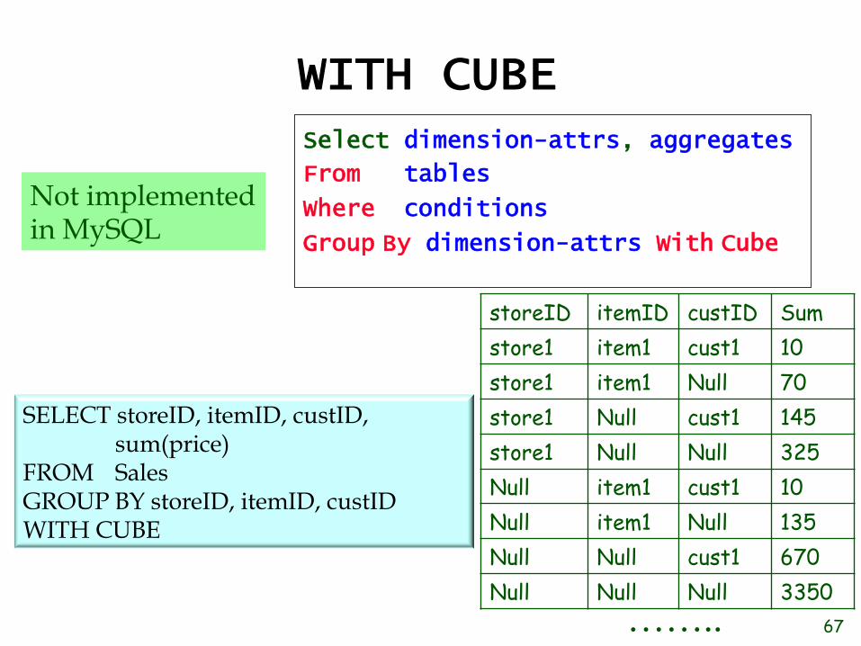
WITH CUBE Select dimension-attrs, aggregates
From tables
Where conditions
Group By dimension-attrs With Cube
storeID itemID custID Sum store1 item1 cust1 10 store1 item1 Null 70 store1 Null cust1 145 store1 Null Null 325 Null item1 cust1 10 Null item1 Null 135 Null Null cust1 670 Null Null Null 3350
SELECT storeID, itemID, custID, sum(price)
FROM Sales GROUP BY storeID, itemID, custID WITH CUBE
……..
Not implemented in MySQL

68
WITH ROLLUP
❖ Can be used in dimensions that are organized in a hierarchy:
State County city Sum CA Santa Clara Palo Alto 325 CA Santa Clara Mountain view 805 CA Santa Clara Null 1130 CA Null Null 1980 Null Null Null 3350
Select dimension-attrs, aggregates
From tables
Where conditions
Group By dimension-attrs With Rollup
County
City
State
SELECT state, county, city, sum(price) FROM Sales F, Store S WHERE F.storeID = S.storeID GROUP BY state, county, city WITH ROLLUP
……..

69
WITH CUBE Example Implemented WITH ROLLUP
❖ Implement the WITH CUBE operator using the WITH ROLLUP operator
SELECT storeID, itemID, custID, sum(price) FROM Sales GROUP BY storeID, itemID, custID with rollup UNION SELECT storeID, itemID, custID, sum(price) FROM Sales GROUP BY itemID, custID, storeID with rollup UNION SELECT storeID, itemID, custID, sum(price) FROM Sales GROUP BY custID, storeID, itemID with rollup;

70
Clicker Question ❖ Consider a fact table Facts(D1,D2,D3,x), and the following three
queries:
❖ Suppose attributes D1, D2, and D3 have n1, n2, and n3 different values respectively, and assume that each possible combination of values appears at least once in table Facts. Pick the one tuple (a,b,c,d,e,f) in the list below such that when n1=a, n2=b, and n3=c, then the result sizes of queries Q1, Q2, and Q3 are d, e, and f respectively.
❖ A: (2, 2, 2, 8, 64, 15) ❖ B: (5, 4, 3, 60, 64, 80) ❖ C: (5, 10, 10, 500, 726, 556) ❖ D: (4, 7, 3, 84, 160, 84)
Q1: Select D1,D2,D3,Sum(x) From Facts Group By D1,D2,D3 Q2: Select D1,D2,D3,Sum(x) From Facts Group By D1,D2,D3 with cube Q3: Select D1,D2,D3,Sum(x) From Facts Group By D1,D2,D3 with rollup
Hint: It may be helpful to first write formulas describing how d, e, and f depend on a, b, and c.

71
Clicker Question ❖ Consider a fact table Facts(D1,D2,D3,x), and the following three
queries:
❖ Suppose attributes D1, D2, and D3 have n1, n2, and n3 different values respectively, and assume that each possible combination of values appears at least once in table Facts. Pick the one tuple (a,b,c,d,e,f) in the list below such that when n1=a, n2=b, and n3=c, then the result sizes of queries Q1, Q2, and Q3 are d, e, and f respectively.
❖ A: (2, 2, 2, 8, 64, 15) ❖ B: (5, 4, 3, 60, 64, 80) ❖ C: (5, 10, 10, 500, 726, 556) ❖ D: (4, 7, 3, 84, 160, 84)
Q1: Select D1,D2,D3,Sum(x) From Facts Group By D1,D2,D3 Q2: Select D1,D2,D3,Sum(x) From Facts Group By D1,D2,D3 with cube Q3: Select D1,D2,D3,Sum(x) From Facts Group By D1,D2,D3 with rollup
d = a*b*c e = a*b*c + a*b + a*c + b*c + a + b +c +1 e = (a+1)*(b+1)*(c+1) f = a*b*c + a*b + a + 1

72
“Date” or “Time” Dimension ❖ Date or Time is a special kind of
dimension.
❖ It has some special and useful OLAP functions.
◆ e.g., durations or time spans, fiscal years, calendar years, and holidays
◆ Business intelligence reports often deal with time-related queries such as comparing the profits from this quarter to the previous quarter … or to the same quarter in the previous year.
TIMES
week month
date
year
quarter
73
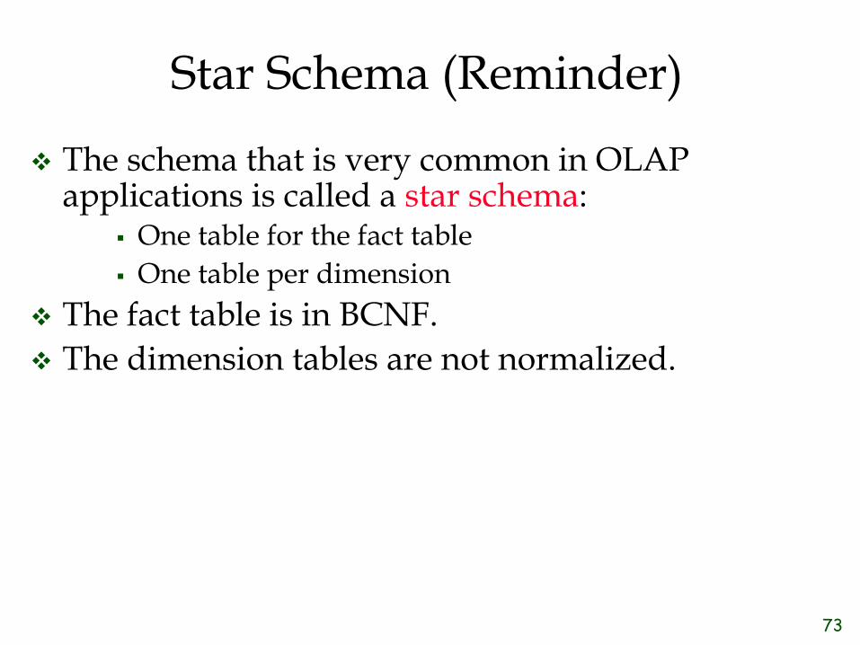
Star Schema (Reminder)
v The schema that is very common in OLAP applications is called a star schema:
§ One table for the fact table § One table per dimension
v The fact table is in BCNF. v The dimension tables are not normalized.

74
Snowflake Schema v The alternative organization is a snowflake schema:
§ each dimension is normalized into a set of tables
§ usually, one table per level of hierarchy, per dimension v Example: TIMES table would be split into:
§ TIMES(timeid, date) § DWEEK(date, week) § DMONTH(date, month)
v Snowflake schema features: § Query formulation is inherently more complex (possibly many joins
per dimension).
v Neither schema is fully satisfactory for OLAP applications. v The star schema is more popular, and is gaining interest.

75
Snowflake Schema example
Source: http://en.wikipedia.org/wiki/Snowflake_schema

76
Star vs. Snowflake Star Snowflake
Ease of maintenance
Has redundant data and hence is less easy to maintain/change
No redundancy, schemas are easier to maintain and change.
Ease of Use Lower complex query writing; easier to understand
More complex queries and hence less easy to understand
Query Performance
Fewer foreign keys and hence shorter query execution time (faster)
More foreign keys and hence longer query execution time (slower)
Joins Fewer Joins More Joins
Dimension table A single dimension table for each dimension
May have more than one dimension table for each dimension
When to use Star schema is the default choice When dimension table is relatively big in size, or we expect a lot of updates
Normalization Dimension Tables are not Normalized
Dimension Tables are Normalized

77
Measures in Fact Tables ❖ Additive facts are measurements in a fact table that
can be added across all the dimensions. e.g., Price ❖ Semi-additive facts are numeric facts that can be
added along some dimensions in a fact table but not others. – balance amounts are common semi-additive facts
because they are additive across all dimensions except time.
❖ Non-additive facts cannot logically be added between rows. – Ratios and percentages – A good approach for non-additive facts is to store the
fully additive components and later compute the final non-additive fact.
78
Factless Fact Tables ❖ Factless fact table: A fact table that has no facts but
captures certain many-to-many relationships between the dimension keys. It’s most often used to represent events or to provide coverage information that does not appear in other fact tables.

79
Factless Fact Table Example
Source: The Data Warehouse Toolkit textbook

80
Multidimensional Data Model
❖ Multidimensional data can be stored in one of 3 ways (modes): – ROLAP (relational online analytical processing)
◆ We access the data in a relational database and generate SQL queries to calculate information at the appropriate level when an end user requests it.
– MOLAP (multidimensional online analytical processing) ◆ Requires the pre-computation and storage of
information in the cube — the operation known as processing. Most MOLAP solutions store such data in an optimized multidimensional array storage, rather than in a relational database.

81
MOLAP vs. ROLAP
MOLAP ROLAP
Data Compression
Can require up to 50% less disk space. A special technique is used for storing sparse cubes.
Requires more disk space
Query Performance
Fast query performance due to optimized storage, multidimensional indexing and caching
Not suitable when the model is heavy on calculations; this doesn’t translate well into SQL.
Data latency Data loading can be quite lengthy for large data volumes. This is usually remedied by doing only incremental processing.
As data always gets fetched from a relational source, data latency is small or none.
handling non-aggregatable facts
Tends to suffer from slow performance when dealing with textual descriptions
Better at handling textual descriptions

82
Which Storage Mode is Recommended? ❖ Almost always, choose MOLAP. ❖ Choose ROLAP if one or more of these are true:
– There is a very large number of members in a dimension—typically hundreds of millions of members.
– The dimension data is frequently changing. – You need real-time access to current data (as opposed to
historical data). – You don’t want to duplicate data.
◆ Reference: [Harinath, et al., 2009]
❖ HOLAP (hybrid online analytical processing) is a combination of ROLAP and MOLAP, which allows storing part of the data in a MOLAP store and another part of the data in a ROLAP store, allowing us to exploit the advantages of each.

83
Finding Answers Quickly
❖ Large datasets and complex queries mean that we’ll need improved querying capabilities – Materializing views – Finding Top N Queries – Using Online aggregation

84
Queries over Views
Create view TshirtSales AS SELECT category, county, gender, price FROM Sales F, Store S, Customer C, Item I WHERE F.storeID = S.storeID AND F.custID = C.custID AND F.itemID = I.itemID ANDcategory = 'Tshirt'
SELECT category, county, gender, SUM(price) From TshirtSales GROUP BY category, county, gender; SELECT category, county, gender, SUM(price) FROM ( SELECT category, county, gender, price FROM Sales F, Store S, Customer C, Item I WHERE F.storeID = S.storeID AND F.custID = C.custID AND F.itemID = I.itemID AND category = 'Tshirt') AS R GROUP BY category, county, gender;
View
Query
Modified Query
❖ How does using a view work?

85
Materializing Views ❖ We can answer a query on a view by using the query
modification technique. – Decision support activities require queries against complex
view definitions to be computed quickly. – Sophisticated optimization and evaluation techniques are
not enough since OLAP queries are typically aggregate queries that require joining huge tables.
❖ Pre-computation is essential for interactive response times.
❖ A view whose tuples are stored in the database is said to be materialized.

86
Issues in View Materialization (1) ❖ Which views should we materialize? ❖ Based on size estimates for the views, suppose we
figure out there is space for k views to be materialized. Which ones should we materialize?
– The goal is to selectively and strategically materialize a small set of carefully chosen views to answer most of the queries quickly.
❖ Fact: Selecting k views to materialize such that the average time taken to evaluate all views of a lattice is minimized is a NP-hard problem.

87
Maximum Coverage Problem Example ❖ Given 9 ground facts/elements, 6 subsets, and a value
for k, find the k subsets (e.g., k = 3) that between them cover as many ground elements as possible.
❖ Maximum Coverage problem has a structure similar to finding the top k views. We can find approximately optimal solutions quickly for both.
Difference between a NP-hard problem and a problem that you solve efficiently (polynomial time) is like the difference between solving a Sudoku puzzle vs. checking whether a given solution is valid.

88
HRU Algorithm
❖ The number associated with each node represents the number of rows in that view (in millions)
❖ Initial state has only the top most view materialized
{S, T, C} 6M
{S, T} 0.8 M {S, C} 6M {T, C} 6M
{S} 0.01M {T} 0.2M {C} 0.1M
{} 1
❖ HRU [Harinarayan, Rajaraman, and Ullman, 1996]—SIGMOD Best Paper award—is a greedy algorithm that does not guarantee an optimal solution, though it usually produces a good solution. This solution is a good trade-off in terms of the space used and the average time to answer an OLAP query.

89
Benefit of Materializing a View
❖ The number associated with each node represents the number of rows in that view (in millions)
❖ Initial state has only the top most view materialized
{S, T, C} 6M
{S, T} 0.8 M {S, C} 6M {T, C} 6M
{S} 0.01M {T} 0.2M {C} 0.1M
{} 1
❖ Define the benefit (savings) of view v relative to S as B(v,S). B(v, S) = 0
For each w ≦ v u = view of least cost in S such that w ≦ u if C(v) < C(u) then Bw = C(v) – C(u) else Bw = 0 B(v,S) = B(v,S) + Bw end
S = set of views selected for materialization b ≦ a means b is a descendant of a (including itself)
C(v) = cost of view v, which we’re approximating by its size

90
Benefit of Materializing a View
❖ The number associated with each node represents the number of rows in that view (in millions)
❖ Initial state has only the top most view materialized
❖ Define the benefit (savings) of view v relative to S as B(v,S). B(v, S) = 0
For each w ≦ v u = view of least cost in S such that w ≦ u if C(v) < C(u) then Bw = C(v) – C(u) else Bw = 0 B(v,S) = B(v,S) + Bw end
Example S = {S, T, C}, v = {S, T} B{S, T} = 5.2 M B{S} = 5.2 M B{T} = 5.2 M B{} = 5.2 M B(v,S) = 5.2M *4
{S, T, C} 6M
{S, T} 0.8 M {S, C} 6M {T, C} 6M
{S} 0.01M {T} 0.2M {C} 0.1M
{} 1

91
Finding the Best k Views to Materialize
❖ The number associated with each node represents the number of rows in that view (in millions)
❖ Initial state has only the top most view materialized
❖ A greedy algorithm for finding the best k views to materialize S = {top view}
for i=1 to k do begin select v ⊄ S such that B(v,S) is maximized S = S union {v} end
{S, T, C} 6M
{S, T} 0.8 M {S, C} 6M {T, C} 6M
{S} 0.01M {T} 0.2M {C} 0.1M
{} 1

92
HRU Algorithm Example
❖ For k=2, other than {S, T, C}, {S, T} and {C} will be materialized.
{S, T, C} 6M
{S, T} 0.8 M {S, C} 6M {T, C} 6M
{S} 0.01M {T} 0.2M {C} 0.1M
{} 1
View 1st choice 2nd choice {S, T} (6-0.8)M *4 = 20.8M
{S, C} (6-6) *4 = 0 (6-6) *2 = 0
{T, C} (6-6) *4 = 0 (6-6) *2 = 0
{S} (6-0.01) M*2 = 11.98M (0.8-0.01)M*2 = 1.58M
{T} (6-0.2) M*2 = 11.6M (0.8-0.2)M*2 = 1.2M
{C} (6-0.1) M*2 = 11.8M (6-0.1)M + (0.8–0.1)M = 6.6M
{} 6M – 1 0.8M – 1

93
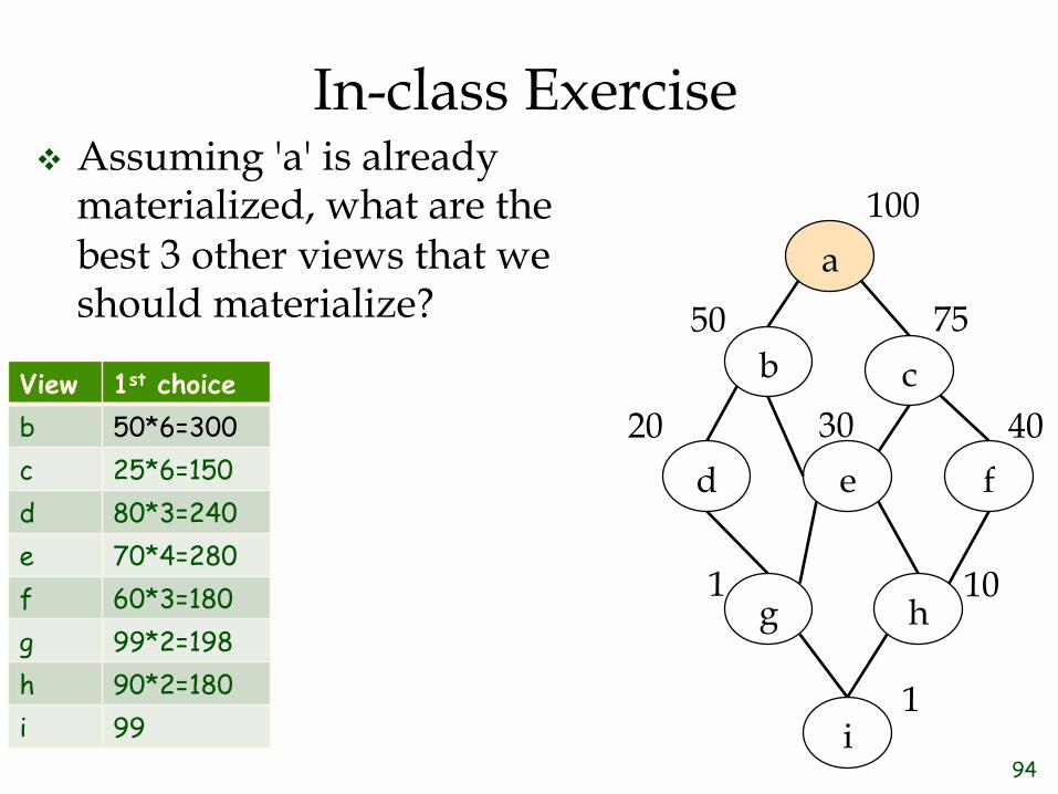
In-class Exercise ❖ Assuming 'a' is already
materialized, what are the best 3 other views that we should materialize?
a
b c
d e f
g h
i
100
75
40
10
1
50
20 30
1
94
In-class Exercise ❖ Assuming 'a' is already
materialized, what are the best 3 other views that we should materialize?
View 1st choice b 50*6=300 c 25*6=150 d 80*3=240 e 70*4=280 f 60*3=180 g 99*2=198 h 90*2=180 i 99
a
b c
d e f
g h
i
100
75
40
10
1
50
20 30
1

95
In-class Exercise ❖ Assuming 'a' is already
materialized, what are the best 3 other views that we should materialize?
View 1st choice b 50*6=300 c 25*6=150 d 80*3=240 e 70*4=280 f 60*3=180 g 99*2=198 h 90*2=180 i 99
a
b c
d e f
g h
i
100
75
40
10
1
50
20 30
1

96
In-class Exercise ❖ Assuming 'a' is already
materialized, what are the best 3 other views that we should materialize?
View 1st choice 2nd choice b 50*6=300 c 25*6=150 25*2=50 d 80*3=240 30*3=90 e 70*4=280 20*4=80 f 60*3=180 60+10*2=80 g 99*2=198 49*2=98 h 90*2=180 40*2=80 i 99 49
a
b c
d e f
g h
i
100
75
40
10
1
50
20 30
1

97
In-class Exercise ❖ Assuming 'a' is already
materialized, what are the best 3 other views that we should materialize?
View 1st choice 2nd choice b 50*6=300 c 25*6=150 25*2=50 d 80*3=240 30*3=90 e 70*4=280 20*4=80 f 60*3=180 60+10*2=80 g 99*2=198 49*2=98 h 90*2=180 40*2=80 i 99 49
a
b c
d e f
g h
i
100
75
40
10
1
50
20 30
1

98
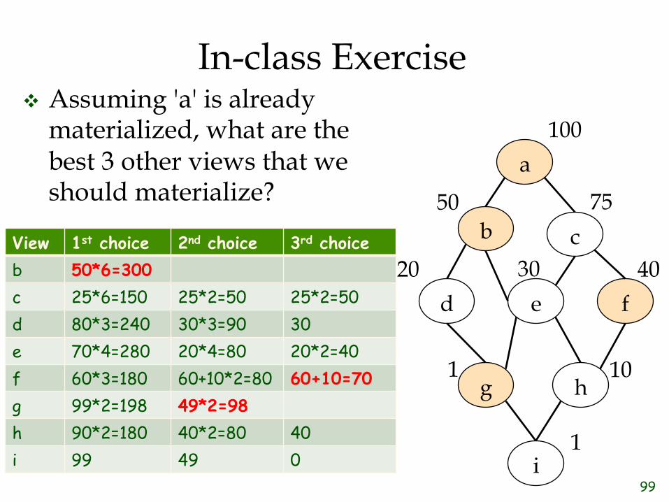
In-class Exercise ❖ Assuming 'a' is already
materialized, what are the best 3 other views that we should materialize?
View 1st choice 2nd choice 3rd choice b 50*6=300 c 25*6=150 25*2=50 25*2=50 d 80*3=240 30*3=90 30 e 70*4=280 20*4=80 20*2=40 f 60*3=180 60+10*2=80 60+10=70 g 99*2=198 49*2=98 h 90*2=180 40*2=80 40 i 99 49 0
a
b c
d e f
g h
i
100
75
40
10
1
50
20 30
1
99
In-class Exercise ❖ Assuming 'a' is already
materialized, what are the best 3 other views that we should materialize?
View 1st choice 2nd choice 3rd choice b 50*6=300 c 25*6=150 25*2=50 25*2=50 d 80*3=240 30*3=90 30 e 70*4=280 20*4=80 20*2=40 f 60*3=180 60+10*2=80 60+10=70 g 99*2=198 49*2=98 h 90*2=180 40*2=80 40 i 99 49 0
a
b c
d e f
g h
i
100
75
40
10
1
50
20 30
1

100
Using the Materialized Views ❖ Once we have chosen a set
of views, we need to consider how they can be used to answer queries on other views.
❖ What is the best way to answer queries on view ‘h’?
a
b c
d e f
g h
i
100
75
40
10
1
50
20 30
1
101
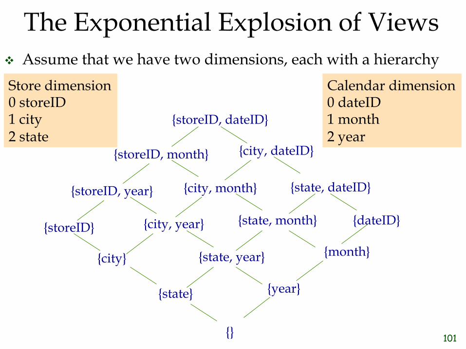
Calendar dimension 0 dateID 1 month 2 year
The Exponential Explosion of Views ❖ Assume that we have two dimensions, each with a hierarchy
Store dimension 0 storeID 1 city 2 state
{}
{year}
{month}
{storeID}
{state}
{city}
{dateID}
{storeID, dateID}
{storeID, month}
{storeID, year}
{city, dateID}
{city, month}
{city, year}
{state, dateID}
{state, month}
{state, year}

102
Issues in View Materialization (2) ❖ What indexes should we build on the materialized
views? – No index is good for all queries.
❖ Consider the ItemCustSales view, which involves a join of Item, Customer, and Sales. Let’s assume that we use (category, gender, price) as our index.
SELECT gender, sum(price) FROM Sales F, Customer C, Item I Where F.custID = C.custID AND F.itemID = I.itemID AND category = 'T-shirt' GROUP BY gender
SELECT category, sum(price) FROM Sales F, Customer C, Item I Where F.custID = C.custID AND F.itemID = I.itemID AND gender = 'M' GROUP BY category
Index on pre-computed view is a good idea
Index is less useful (must scan entire index)

103
Issues in View Materialization (3) ❖ How do we maintain views incrementally without
re-computing them from scratch? v Two steps:
§ Identify the changes to the view when the data changes.
§ Apply only those changes to the materialized view.
§ There may be challenges in refreshing, especially if the base tables are distributed across multiple locations.

104
Issues in View Materialization (4)
❖ How should we refresh and maintain a materialized view when an underlying table is modified?
❖ Maintenance policy: Controls when we refresh § Immediate: As part of the transaction that modifies the
underlying data tables + Materialized view is always consistent - Updates are slow
§ Deferred: Some time later, in a separate transaction - View is inconsistent for a while + Can scale to maintain many views without slowing updates

105
Deferred Maintenance
❖ Three flavors: – Lazy: Delay refresh until next query on view; then refresh
before answering the query. ◆ This approach slows down queries rather than
updates, in contrast to immediate maintenance.
– Periodic (Snapshot): Refresh periodically. Queries possibly answered using outdated version of view tuples. Also widely used in asynchronous replication in distributed databases
– Event-based (Forced): e.g., Refresh after a fixed number of updates to underlying data tables

106
Top N Queries ❖ For complex queries, users like to get an approximate
answer quickly and keep refining their query.
❖ Top N Queries: If you want to find the 10 (or so) cheapest items, it would be nice if the DBMS could avoid computing the costs of all items before sorting to determine the 10 cheapest. – Idea: Guess a cost c such that the 10 cheapest items all
cost less than c, and that not too many more cost less; then, add the selection “cost < c” and evaluate the query. ◆ If the guess is right, great; we avoid computation for
items that cost more than c. ◆ If the guess is wrong, then we need to reset the
selection and re-compute the query.

107
Top N Queries
❖ “OPTIMIZE FOR” construct is not in SQL:1999, but supported in DB2 or Oracle 9i
❖ Cut-off value c is chosen by the optimizer
SELECT P.pid, P.pname, S.sales FROM Sales S, Products P WHERE S.pid=P.pid AND S.locid=1 AND S.timeid=3 ORDER BY S.sales DESC OPTIMIZE FOR 10 ROWS;
SELECT P.pid, P.pname, S.sales FROM Sales S, Products P WHERE S.pid=P.pid AND S.locid=1 AND S.timeid=3
AND S.sales > c ORDER BY S.sales DESC;
v Some DBMSs (e.g., DB2) offer special features for this.
108
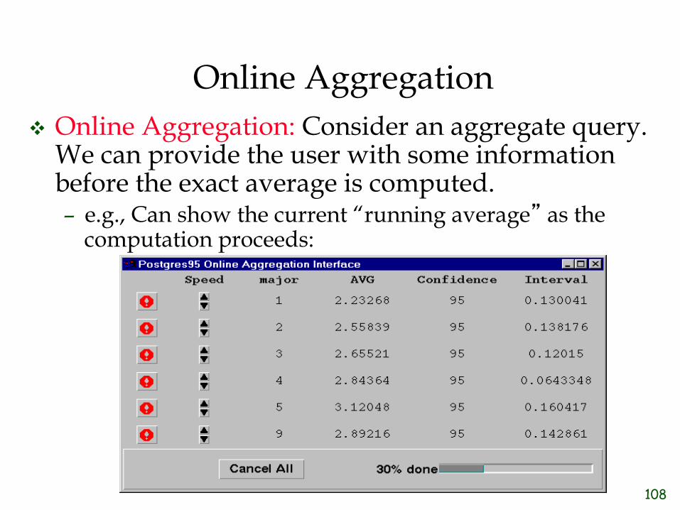
Online Aggregation ❖ Online Aggregation: Consider an aggregate query.
We can provide the user with some information before the exact average is computed. – e.g., Can show the current “running average” as the
computation proceeds:

109
Multidimensional Expressions (MDX) ❖ Multidimensional Expressions (MDX) is a query
language for OLAP databases, much like SQL is a query language for relational databases.
v Like SQL, MDX has SELECT, FROM, and WHERE clauses (and others).
v Sample MDX syntax:
v You will be running MDX queries in the tutorial.
SELECT <content> ON COLUMNS, <content> ON ROWS, <content> ON PAGES
FROM <name_of_cube> WHERE
110
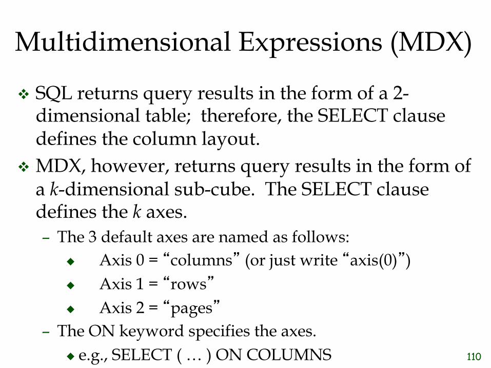
Multidimensional Expressions (MDX)
v SQL returns query results in the form of a 2-dimensional table; therefore, the SELECT clause defines the column layout.
v MDX, however, returns query results in the form of a k-dimensional sub-cube. The SELECT clause defines the k axes. – The 3 default axes are named as follows:
◆ Axis 0 = “columns” (or just write “axis(0)”) ◆ Axis 1 = “rows” ◆ Axis 2 = “pages”
– The ON keyword specifies the axes. ◆ e.g., SELECT ( … ) ON COLUMNS

111
Multidimensional Expressions (MDX)
❖ The queries can be simple or complex.
❖ MDX allows you to restrict analysis/calculations to a particular sub-cube of the overall data cube. This is useful for slice and dice operations. – e.g., You may wish to focus only the set of T-shirts that
were sold to Males.
❖ MDX queries can be optimized, similar in spirit to the way SQL queries are optimized; but, the process is more complex.

112
Learning Goals Revisited v Compare and contrast OLAP and OLTP processing (e.g., focus,
clients, amount of data, abstraction levels, concurrency, and accuracy).
v Explain the ETL tasks (i.e., extract, transform, load) for data warehouses.
v Explain the differences between a star schema design and a snowflake design for a data warehouse, including potential tradeoffs in performance.
v Argue for the value of a data cube in terms of: the type of data in the cube (numeric, categorical, counts, sums) and the goals of OLAP (e.g., summarization, abstractions).
v Estimate the complexity of a data cube in terms of the number of views that a given fact table and set of dimensions could generate, and provide some ways of managing this complexity.

113
Learning Goals Revisited (cont.) v Given a multidimensional cube, write regular SQL queries that
perform roll-up, drill-down, slicing, dicing, and pivoting operations on the cube.
v Use the SQL:1999 standards for aggregation (e.g., GROUP BY CUBE) to efficiently generate the results for multiple views.
v Explain why having materialized views is important for a data warehouse.
v Determine which set of views are most beneficial to materialize.
v Given an OLAP query and a set of materialized views, determine which views could be used to answer the query more efficiently than the fact table (base view).
v Define and contrast the various methods and policies for materialized view maintenance.