CPS 270: Artificial Intelligencehttp://www.cs.duke.edu/courses/fall08/cps270/

Markov processes and Hidden Markov Models (HMMs)

Instructor: Vincent Conitzer

Motivation• The Bayes nets we considered so far were

static: they referred to a single point in time

– E.g., medical diagnosis

• Agent needs to model how the world evolves

– Speech recognition software needs to process

speech over time

– Artificially intelligent software assistant needs to

keep track of user’s intentions over time

– … … …

Markov processes• We have time periods t = 0, 1, 2, …

• In each period t, the world is in a certain state St

• The Markov assumption: given St, St+1 is independent of all

Si with i < t

– P(St+1 | S1, S2, …, St) = P(St+1 | St)

– Given the current state, history tells us nothing more about the

future

S1 S2 S3 … St …• Typically, all the CPTs are the same:

• For all t, P(St+1 = j | St = i) = aij (stationarity assumption)

Weather example• St is one of {s, c, r} (sun, cloudy, rain)

• Transition probabilities:

s

c r

.1

.2

.6

.3.4

.3

.3

.5

.3

not a Bayes net!

• Also need to specify an initial distribution P(S0)

• Throughout, assume P(S0 = s) = 1

Weather example…

s

c r

.1

.2

.6

.3.4

.3

.3

.5

.3

• What is the probability that it rains two days from now? P(S2 = r)

• P(S2 = r) = P(S2 = r, S1 = r) + P(S2 = r, S1 = s) + P(S2 = r, S1 = c) = .1*.3 + .6*.1 + .3*.3 = .18

Weather example…

s

c r

.1

.2

.6

.3.4

.3

.3

.5

.3

• What is the probability that it rains three days from now?

• Computationally inefficient way: P(S3 = r) = P(S3 = r, S2 = r, S1 = r) + P(S3 = r, S2 = r, S1 = s) + …

• For n periods into the future, need to sum over 3n-1 paths

Weather example…

s

c r

.1

.2

.6

.3.4

.3

.3

.5

.3

• More efficient:

• P(S3 = r) = P(S3 = r, S2 = r) + P(S3 = r, S2 = s) + P(S3 = r, S2 = c) = P(S3 = r | S2 = r)P(S2 = r) + P(S3 = r | S2 = s)P(S2 = s) + P(S3 = r | S2 = c)P(S2 = c)

• Only hard part: figure out P(S2)

• Main idea: compute distribution P(S1), then P(S2), then P(S3)

• Linear in number of periods!

example on board

Stationary distributions• As t goes to infinity, “generally,” the distribution

P(St) will converge to a stationary distribution

• A distribution given by probabilitiesπi (where i is a

state) is stationary if:

P(St = i) =πi means that P(St+1 = i) =πi

• Of course,

P(St+1 = i) = Σj P(St+1 = i, St = j) = Σj P(St = j) aji

• So, stationary distribution is defined by

πi = Σj πj aji

Computing the stationary distribution

• πs = .6πs + .4πc + .2πr

• πc = .3πs + .3πc + .5πr

• πr = .1πs + .3πc + .3πr

s

c r

.1

.2

.6

.3.4

.3

.3

.5

.3

Restrictiveness of Markov models• Are past and future really independent given current state?

• E.g., suppose that when it rains, it rains for at most 2 days

S1 S2 S3 S4 …• Second-order Markov process

• Workaround: change meaning of “state” to events of last 2 days

S1, S2 …S2, S3 S3, S4 S4, S5

• Another approach: add more information to the state

• E.g., the full state of the world would include whether the sky is full of water– Additional information may not be observable

– Blowup of number of states…

Hidden Markov models (HMMs)• Same as Markov model, except we cannot see the

state

• Instead, we only see an observation each period,

which depends on the current state

S1 S2 S3 … St …

• Still need a transition model: P(St+1 = j | St = i) = aij

• Also need an observation model: P(Ot = k | St = i) = bik

O1 O2 O3 … Ot …

Weather example extended to HMM • Transition probabilities:

s

c r

.1

.2

.6

.3.4

.3

.3

.5

.3

• Observation: labmate wet or dry

• bsw = .1, bcw = .3, brw = .8

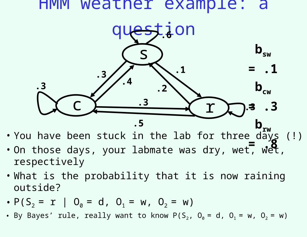
HMM weather example: a question

s

c r

.1

.2

.6

.3.4

.3

.3

.5

.3

• You have been stuck in the lab for three days (!)• On those days, your labmate was dry, wet, wet,

respectively• What is the probability that it is now raining outside?

• P(S2 = r | O0 = d, O1 = w, O2 = w)• By Bayes’ rule, really want to know P(S2, O0 = d, O1 = w, O2 = w)

bsw = .1

bcw = .3

brw = .8

Solving the question

s

c r

.1

.2

.6

.3.4

.3

.3

.5

.3

• Computationally efficient approach: first compute

P(S1 = i, O0 = d, O1 = w) for all states i

• General case: solve for P(St, O0 = o0, O1 = o1, …, Ot = ot) for t=1, then t=2, … This is called monitoring

• P(St, O0 = o0, O1 = o1, …, Ot = ot) = Σst-1 P(St-1 = st-1, O0 =

o0, O1 = o1, …, Ot-1 = ot-1) P(St | St-1 = st-1) P(Ot = ot | St)

bsw = .1

bcw = .3

brw = .8

Predicting further out

s

c r

.1

.2

.6

.3.4

.3

.3

.5

.3

• You have been stuck in the lab for three days• On those days, your labmate was dry, wet, wet,

respectively• What is the probability that two days from now it

will be raining outside?

• P(S4 = r | O0 = d, O1 = w, O2 = w)

bsw = .1

bcw = .3

brw = .8

Predicting further out, continued…

s

c r

.1

.2

.6

.3.4

.3

.3

.5

.3

• Want to know: P(S4 = r | O0 = d, O1 = w, O2 = w)

• Already know how to get: P(S2 | O0 = d, O1 = w, O2 = w)

• P(S3 = r | O0 = d, O1 = w, O2 = w) =

Σs2 P(S3 = r, S2 = s2 | O0 = d, O1 = w, O2 = w)

Σs2 P(S3 = r | S2 = s2)P(S2 = s2 | O0 = d, O1 = w, O2 = w)

• Etc. for S4

• So: monitoring first, then straightforward Markov process updates

bsw = .1

bcw = .3

brw = .8

Integrating newer information

s

c r

.1

.2

.6

.3.4

.3

.3

.5

.3

• You have been stuck in the lab for four days (!)• On those days, your labmate was dry, wet, wet, dry

respectively• What is the probability that two days ago it was

raining outside? P(S1 = r | O0 = d, O1 = w, O2 = w, O3 = d)– Smoothing or hindsight problem

bsw = .1

bcw = .3

brw = .8

Hindsight problem continued…

s

c r

.1

.2

.6

.3.4

.3

.3

.5

.3

• Want: P(S1 = r | O0 = d, O1 = w, O2 = w, O3 = d)

• “Partial” application of Bayes’ rule:

P(S1 = r | O0 = d, O1 = w, O2 = w, O3 = d) =

P(S1 = r, O2 = w, O3 = d | O0 = d, O1 = w) /

P(O2 = w, O3 = d | O0 = d, O1 = w)

• So really want to know P(S1, O2 = w, O3 = d | O0 = d, O1 = w)

bsw = .1

bcw = .3

brw = .8

Hindsight problem continued…

s

c r

.1

.2

.6

.3.4

.3

.3

.5

.3

• Want to know P(S1 = r, O2 = w, O3 = d | O0 = d, O1 = w)

• P(S1 = r, O2 = w, O3 = d | O0 = d, O1 = w) =

P(S1 = r | O0 = d, O1 = w) P(O2 = w, O3 = d | S1 = r)

• Already know how to compute P(S1 = r | O0 = d, O1 = w)

• Just need to compute P(O2 = w, O3 = d | S1 = r)

bsw = .1

bcw = .3

brw = .8

Hindsight problem continued…

s

c r

.1

.2

.6

.3.4

.3

.3

.5.3

• Just need to compute P(O2 = w, O3 = d | S1 = r)

• P(O2 = w, O3 = d | S1 = r) =

Σs2 P(S2 = s2, O2 = w, O3 = d | S1 = r) =

Σs2 P(S2 = s2 | S1 = r) P(O2 = w | S2 = s2) P(O3 = d | S2 = s2)

• First two factors directly in the model; last factor is a “smaller” problem of the same kind

• Use dynamic programming, backwards from the future– Similar to forwards approach from the past

bsw = .1

bcw = .3

brw = .8

Backwards reasoning in general• Want to know P(Ok+1 = ok+1, …, Ot = ot | Sk)

• First compute

P(Ot = ot | St-1) =Σst P(St = st | St-1)P(Ot = ot | St = st)

• Then compute

P(Ot = ot, Ot-1 = ot-1 | St-2) =Σst-1 P(St-1 = st-1 | St-2)P(Ot-1 = ot-1 | St-1 = st-1)

P(Ot = ot | St-1 = st-1)

• Etc.

Dynamic Bayes Nets• Everything so far is just doing inference on a special

kind of Bayes net!• So far assumed that each period has one variable

for state, one variable for observation• Often better to divide state and observation up into

multiple variables

NC wind, 1

weather in Durham, 1

weather in Beaufort, 1

NC wind, 2

weather in Durham, 2

weather in Beaufort, 2

…

edges both within a period, and from one period to the next…

Some interesting things we skipped• Finding the most likely sequence of states,

given observations–Not necessary equal to the sequence of most

likely states! (example?)–Viterbi algorithm

• Key idea: for each period t, for every state, keep track of most likely sequence to that state at that period, given evidence up to that period

• Continuous variables• Approximate inference methods

–Particle filtering