CP3 REVISION LECTURE ON - University of Oxford · PDF fileCP3 REVISION LECTURE ON Ordinary diﬀerential equations 1 First order linear equations 2 First order nonlinear equations

CP3 REVISION LECTURE ON

Ordinary differential equations

1 First order linear equations

2 First order nonlinear equations

3 Second order linear equations with constant coefficients

4 Systems of linear ordinary differential equations

BASIC CONCEPTS

• Every differential equation involves a differential operator.Order of a differential operator: order of highest derivative contained in it

• Linearity: differential operator L is linear if

for any two functions f and g

L(αf + βg) = αLf + βLg

with α and β any constants.

• Linearity ⇒ superposition principle:

If f1 and f2 are solutions of Lf = 0, then anylinear combination αf1 + βf2 is also solution.

Lf = 0 homogeneous differential equation

Lf = h(x) 6= 0 inhomogeneous differential equation

• General solution of linear inhomogeneous ODE Lf = h is sum

of a particular solution f0 (the “particular integral”, PI) and the general

solution f1 of the associated homogeneous equation (the

“complementary function”, CF):

f = f0 + f1 ,

i.e., GS = PI + CF .

• Initial conditions:

n initial conditions needed to specify solutionof linear ODE of order n

!"#$%&'#()#&*"+),#&)-.,/'+$&

dGeneral form : ( ) ( )

d

fq x f h x

x+ = .

Look for a function I(x) such that I(x)

df

dx+ I(x)q(x) f !

dIf

dx= I(x)h(x)

0+%)1#,/+1&2,3%'#&

Solution : f (x) =1

I(x)I(x ')h(x ')dx '

x0

x

!

4,$5&%'&$'*6)&

I(x) = eq(x ') dx '

x

!

June 2006

2. Find the general solution of the differential equation

1

x

dy

dx−

y

x2= sinx

[Answ.: x(c− cosx)]

June 2008

4. Solve the differential equation

x(x+ 1)dy

dx+ y = x(x+ 1)2e−x2

[Answ.: (c− e−x2

/2)(x+ 1)/x]

September 2009


xdy

dx+ 2y = cosx

[Answ.: (cosx+ x sinx+ c)/x2]

!"#$%&'#()#&*'*+"*),#&)-.,/'*$&

0+%1'.21&*'&2)*)#,+&3)%1'(&4'#&$'+./'*&"$&,5,"+,6+)7&%1)#)&,#)&$)5)#,+&8,$)$&'4&&

91:$"8,++:&#)+)5,*%&*'*+"*),#&)-.,/'*$&;1"81&8,*&6)&$'+5)(&,*,+:/8,++:&<&

=)9,#,6+)&)-.,/'*$&d ( )

d ( )

y f x

x g y= ( ) ( )g y dy f x dx=! !='+./'*&<&

d( )

d

yf ax by

x= +

0+3'$%&$)9,#,6+)&)-.,/'*$&

z ax by= +>1,*2)&5,#",6+)$&<& z ax by= +

dz

dx= a + bf (z) Separable

d( )

d

yf y x

x= / .?'3'2)*)'.$&)-.,/'*$&

y = vx>1,*2)&5,#",6+)$&<&

dv

dx=

1

x( f (v) ! v) Separable

!"#"$%&%"'()*'+),"-)."&(+/&+()2 1

2

dy x y

dx x y

+ +=

+ +

Change variables : x = x '+ a, y = y '+ b

dy '

dx '=

x '+ 2y '+1+ a + 2b

x '+ y '+ 2 + a + b=

x '+ 2y '

x '+ y ', a = !3, b = 1 Homogeneous

d( ) ( ) , 1

d

nyP x y Q x y n

x+ = !01%)2%-&"'334)%5'/6"&)

Change variables : z = y1!n

dz

dx+ (1! n)P(x)z = (1! n)Q(x), First order linear

Exact equations :dy

dx= −

∂φ/∂x

∂φ/∂y

for a given function φ(x, y)

• Then solution is determined by

φ(x, y) = constant .

June 2005


2dy

dx=

y(x+ y)

x2“homogeneous”

[Answ.: y = x/(1− c√x)]

June 2007

8. Find the general solution to the differential equation

ydy

dx=

x

4x+ 3“separable”

[Answ.: y2 = c+ x/2− (3/8) ln(4x+3)]

September 2009


dy

dx=

x+ y

1− x− y“almost separable”

[Answ.: y− (x+ y)2/2 = c]


dy

dx+ xy = xy2 “Bernoulli”

[Answ.: y = 1/(1 + cex2/2)]


(2y − x cos y)dy

dx= x+ sin y “exact”

[Answ.: x sin y − y2 + x2/2 = c]

GEOMETRICAL INTERPRETATION OF SOLUTIONS

• General solution of a first-order ODE y′ = f(x, y)

contains an arbitrary constant: y = (x, c)

⊲ one curve in x, y plane for each value of c ⇒ family of curves

Example: y′ = −x/y.

separable equation ⇒∫

y dy = −∫

x dx ⇒ y2/2 = −x2/2 + c

i.e., x2 + y2 = constant : family of circles centered at origin

Fig.1

x

y

Orthogonal family of curves : y′ = −1/f(x, y)

Example : y′ = y/x ⇒ y = cx

SUMMARY ON NONLINEAR FIRST-ORDER ODEs

• No general method of solution for 1st-order ODEs beyond linear case;rather, a variety of techniques that work on a case-by-case basis.

Examples:

i) Bring equation to separated-variables form, that is, y′ = α(x)/β(y);

then equation can be integrated.

Cases covered by this include y′ = ϕ(ax+ by); y′ = ϕ(y/x).

ii) Reduce to linear equation by transformation of variables.

Examples of this include Bernoulli’s equation.

iii) Bring equation to exact-differential form, that is

dy/dx = −M(x, y)/N(x, y) such that M = ∂φ/∂x, N = ∂φ/∂y.

Then solution determined from φ(x, y) = const.

SECOND-ORDER LINEAR ODEs

f ′′ + p(x)f ′ + q(x)f = h(x)

• General solution = PI + CF

• CF = c1u1 + c2u2u1 and u2 linearly independent solutions

of the homogeneous equation

• 2nd-order linear ODEs with constant coefficients:a2f

′′ + a1f′ + a0f = h(x)

⊲ Complementary function CF by solving auxiliary equation

⊲ Particular integral PI by trial function with functional formof the inhomogeneous term

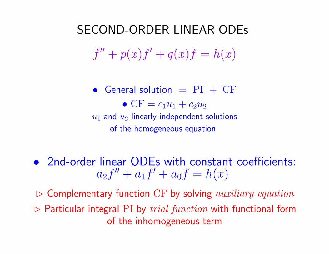
2

2 1 02

d d( )

d d

f fLf a a a f h x

x x= + + = .

!"#$%&'$(&"(')*%"+('",-+.$%'/*01'#$%20+%0'#$"3#*"%02'

4$56)"5"%0+(7'8-%#.$%'

Lf

0= a

2

d2 f

0

dx2+ a

1

df0

dx+ a

0f

0= 0.

Try f

0= e

mx 2

2 1 00a m a m a+ + = .

2

1 1 2 0

2

4

2

a a a am

a±

! ± !" ,

f

0= A

+em+x+ A

!em!x.

9:-;*)*+(7<'",-+.$%'

4$56)"5"%0+(7'8-%#.$%'

=/$'#$%20+%02'$8'*%0">(+.$%'

2

1 2 04 ,0,a a a +! " !

2

2 1 02

d d( )

d d

f fLf a a a f h x

x x= + + = .

!"#$%&'$(&"(')*%"+('",-+.$%'/*01'#$%20+%0'#$"3#*"%02'

4$56)"5"%0+(7'8-%#.$%'

Lf

0= a

2

d2 f

0

dx2+ a

1

df0

dx+ a

0f

0= 0.

Try f

0= e

mx 2

2 1 00a m a m a+ + = .

2

1 1 2 0

2

4

2

a a a am

a±

! ± !" , 9:-;*)*+(7<'",-+.$%'

4$56)"5"%0+(7'8-%#.$%'

2

1 2 04 ,0,a a a +! " !

f

0= Ae

mx+ Bxe

mx

="6"+0"&'($$02'

2

2 1 02

d d( )

d d

f fLf a a a f h x

x x= + + = .

!"#$%&'$(&"(')*%"+('",-+.$%'/*01'#$%20+%0'#$"3#*"%02'

4+(.#-)+('*%0"5(+)'

Lf

1= a

2

d2 f

1

dx2+ a

1

df1

dx+ a

0f1= h.

0 1General solution : f f+

6$78)"7"%0+(9':-%#.$%'

Lf0= a

2

d2 f0

dx2+ a

1

df0

dx+ a

0f0= 0.

June 2006


3d2y

dx2+

dy

dx− 4y = 0

with initial conditions y(0) = 0 and dy/dx(0) = 7.

[Answ.: 3(ex − e−4x/3)]

September 2007


d2y

dt2+ 7

dy

dt+ 12y = 3 exp(2t)

[Answ.: c1e−4t + c2e−3t + e2t/10]

June 2008


d2y

dx2+ 3

dy

dx+ 2y = e−x

[Answ.: c1e−x + c2e−2x + xe−x]

September 2009

10. A mass m is suspended on a spring. Its displacement y as a function of time t isdescribed by the equation

d2y

dt2+ 2γ

dy

dt+ ω2

0y =F0

meiωt ,

where γ, ω0 and F0 are constants. Initially no driving force is present (F0 = 0). De-termine the solution to the equation when γ2 < ω2

0, subject to the initial conditions

y = y0 and dydt

= 0 at t = 0.

The driving force is now applied. Find the time dependence of y at sufficiently longtimes such that all transients have died away. Sketch as a function of ω the amplitudeof y and its phase φ relative to the driving force.

When ω = ω0, show that the average power supplied by the driving force is

Pav =F 2

0

4mγ.

CPSC 4296 4

y′′ + 2γy′ + ω20y = (F0/m) eiωt .

CF (F0 = 0):

Characteristic eq. λ2 + 2γλ+ ω20 = 0 ⇒ λ± = − γ ±

√

γ2 − ω20

γ2 < ω20 : λ± = − γ ± i

√

ω20 − γ2

︸︷︷︸

ω′

So CF = e−γt[A cosω′t+ B sinω′t] .

Initial conditions y(0) = y0, y′(0) = 0

⇒ A = y0, Bω′ − Aγ = 0 ⇒ B = y0γ/ω

′

Thus y(t) = y0e−γt[cosω′t+ (γ/ω′) sinω′t] .

PI (F switched on):

Trial function y = Ceiωt ⇒ C(−ω2 + 2γiω + ω20) = F0/m

So C =F0/m

ω20 − ω2 + 2γiω

= |C|eiφ

where |C| =F0/m

√

(ω20 − ω2)2 + 4γ2ω2

(amplitude)

tanφ =2γω

ω2 − ω20

(phase)

•Power P supplied by the driving force F : P = Fdy

dt

where F = F0eiωt , y(t) = |C|ei(ωt+φ) ,

dy

dt= |C|iωei(ωt+φ) .

• Using the explicit expressions determined previously

for amplitude |C| and phase φ we get

P =ωF 2

0 /m√

(ω20 − ω2)2 + 4γ2ω2

sin(2ωt+ φ) + sinφ

2

where sinφ =tanφ

√

1 + tan2 φ=

2γω√

(ω20 − ω2)2 + 4γ2ω2

• Taking the average power 〈P 〉 (〈sin(2ωt+ φ)〉 = 0)

⇒ 〈P 〉 =γω2F 2

0 /m

(ω20 − ω2)2 + 4γ2ω2

Thus 〈P 〉 =F 20

4mγfor ω2 = ω2

0 .

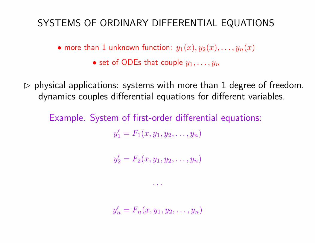
SYSTEMS OF ORDINARY DIFFERENTIAL EQUATIONS

• more than 1 unknown function: y1(x), y2(x), . . . , yn(x)

• set of ODEs that couple y1, . . . , yn

⊲ physical applications: systems with more than 1 degree of freedom.dynamics couples differential equations for different variables.

Example. System of first-order differential equations:

y′1 = F1(x, y1, y2, . . . , yn)

y′2 = F2(x, y1, y2, . . . , yn)

· · ·

y′n = Fn(x, y1, y2, . . . , yn)

♦ Systems of linear ODEs with constant coefficients can be solvedby a generalization of the method seen for single ODE:

General solution = PI + CF

⊲ Complementary function CF by solvingsystem of auxiliary equations

⊲ Particular integral PI from a

set of trial functions

with functional form as the inhomogeneous terms

June 2007

The variables ψ(z) and φ(z) obey thesimultaneous differential equations

3dφ

dz+ 5ψ = 2z

3dψ

dz+ 5φ = 0.

Find the general solution for ψ.

• Differentiating 2nd equation wrt z gives

0 = 3d2ψ

dz2+ 5

dφ

dz= 3

d2ψ

dz2+

5

3(2z − 5ψ)

i.e.d2ψ

dz2−

25

9ψ = −

10

9z

• Solve this 2nd-order linear ODE with constant coefficients:

CF: Auxiliary equation m2 − 25/9 = 0 ⇒ m± = ±5/3.So CF = Ae5z/3 +Be−5z/3.

PI: Trial function ψ0 = C1z + C0 ⇒

−(25/9)C1z − (25/9)C0 = −10/9z⇒ C1 = 2/5 , C0 = 0 ⇒ PI = 2z/5.

General solution for ψ :

ψ(z) = CF + PI = A e5z/3 + B e−5z/3 +2

5z .

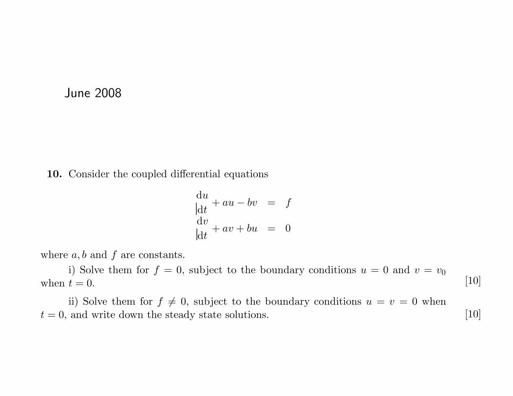
June 2008

10. Consider the coupled differential equations

du

dt+ au − bv = f

dv

dt+ av + bu = 0

where a, b and f are constants.

i) Solve them for f = 0, subject to the boundary conditions u = 0 and v = v0

when t = 0. [10]

ii) Solve them for f "= 0, subject to the boundary conditions u = v = 0 whent = 0, and write down the steady state solutions. [10]

• Using notation D = d/dt,

(D + a)u− bv = f

bu+ (D + a)v = 0

• Apply D + a on 1st eq. and multiply 2nd eq. by b:

(D + a)2u− b(D + a)v = (D + a)f

b2u+ b(D + a)v = 0

• Add the two equations:

[(D + a)2 + b2]u = af

which is 2nd-order ODE with constant coefficients

u′′ + 2au′ + (b2 + a2)u = af .

General solution

CF: Auxiliary equation λ2 + 2aλ+ (b2 + a2) = 0 ⇒ λ± = −a± ib.

So CF = e−at[A cos bt+B sin bt].

PI: Trial function: constant u0 = C ⇒ C = af/(a2 + b2).

General solution for u :

u(t) = CF + PI = e−at[A cos bt+ B sin bt] + af/(a2 + b2) .

General solution for v :

v(t) = b−1[(D + a)u− f ] = e−at[−A sin bt+B cos bt]− bf/(a2 + b2) .

i) f = 0, u(0) = 0 and v(0) = v0 ⇒ A = 0, B = v0

Therefore u(t) = v0e−at sin bt ,

v(t) = v0e−at cos bt .

ii) f 6= 0, u(0) = v(0) = 0 ⇒ A = −af/(a2 + b2), B = bf/(a2 + b2)

Therefore u(t) = f/(a2 + b2)[e−at(−a cos bt+ b sin bt) + a] ,

v(t) = f/(a2 + b2)[e−at(a sin bt+ b cos bt)− b] .

Steady state solutions t→∞:

u = af/(a2 + b2) , v = −bf/(a2 + b2) .

Documents

CP3 REVISION LECTURE ON - University of Oxford · PDF fileCP3 REVISION LECTURE ON Ordinary diﬀerential equations 1 First order linear equations 2 First order nonlinear equations