Embed Size (px)
Citation preview

WELL LOGGING LABORATORY
TECHNICAL REPORT NO. 32
October 2011
Department of Electrical Engineering
Cullen College of Engineering
University of Houston

Technical Report N
o. 32 University of H
ouston 2011

i
WELL LOGGING TECHNICAL REPORT NO. 32
October 2011
All rights reserved
Well Logging Laboratory Department of Electrical and Computer Engineering
University of Houston Houston, Texas 77204-4005
U. S. A.

ii
Research Staff Faculty Dr. Qiming Li, Adjunct Professor
Dr. Kurt M. Strack, Adjunct Professor
Dr. Donald Wilton, Professor
Dr. Richard Liu, Professor
Dr. Ning Yuan, Research Assistant Professor
Post Doctors
Dr. Xiaochun Nie
Research Assistants
Jing Li (Ph. D. Candidate)
Min Wu (Ph.D. Candidate)
Zhijuan Zhang (Ph.D. Candidate)
Fouad Shehab (Master Candidate)
Yajun Kong (M. S. Candidate)
Chang Ming Lin (M. S. Candidate)
Boyuan Yu (Ph.D. Candidate)
Ziting Liu (M. S. Candidate)
Bo Gong (Ph.D. Candidate)
Yinxi Zhang (Ph.D. Candidate)
Jing Wang (Ph.D. Candidate)
Azizuddin Abdul Aziz (Ph.D. Candidate)

iii
Acknowledgment
The authors would like to acknowledge gratefully the financial support and the technical assistance which they have received from the following companies: BP
Chevron E & P Technology Company
ExxonMobil Upstream Research Company
Great Wall Drilling Company
Halliburton Energy Services
Pathfinder Energy Services
Saudi Aramco
Schlumberger Oilfield Services
Statoil
Weatherford
iv
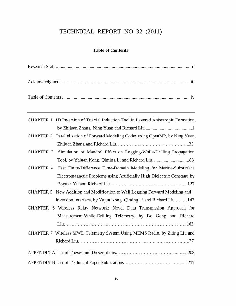
TECHNICAL REPORT NO. 32 (2011)
Table of Contents
Research Staff ..................................................................................................................... ii
Acknowledgment ............................................................................................................... iii
Table of Contents ............................................................................................................... iv
CHAPTER 1 1D Inversion of Triaxial Induction Tool in Layered Anisotropic Formation,
by Zhijuan Zhang, Ning Yuan and Richard Liu.........................................1
CHAPTER 2 Parallelization of Forward Modeling Codes using OpenMP, by Ning Yuan,
Zhijuan Zhang and Richard Liu……………...…..………..….………...32
CHAPTER 3 Simulation of Mandrel Effect on Logging-While-Drilling Propagation
Tool, by Yajuan Kong, Qiming Li and Richard Liu…............................83
CHAPTER 4 Fast Finite-Difference Time-Domain Modeling for Marine-Subsurface
Electromagnetic Problems using Artificially High Dielectric Constant, by
Boyuan Yu and Richard Liu….……………..………...…………….…127
CHAPTER 5 New Addition and Modification to Well Logging Forward Modeling and
Inversion Interface, by Yajun Kong, Qiming Li and Richard Liu.…..…147
CHAPTER 6 Wireless Relay Network: Novel Data Transmission Approach for
Measurement-While-Drilling Telemetry, by Bo Gong and Richard
Liu……………………………………………………………………..162
CHAPTER 7 Wireless MWD Telemetry System Using MEMS Radio, by Ziting Liu and
Richard Liu….…………….…………………………...…………….…177
APPENDIX A List of Theses and Dissertations…………………………………...…...208
APPENDIX B List of Technical Paper Publications…………………………...………217

1D Inversion of Triaxial Induction Tool in Layered Anisotropic Formation
1
CHAPTER 1
1D Inversion of Triaxial Induction Tool in Layered Anisotropic
Formation
Abstract
In this paper, we present a one-dimensional (1-D) inversion algorithm for triaxial
induction logging tools in multi-layered transverse isotropic (TI) formation. A non-linear
least-square model based on Gauss-Newton algorithm is used in the inversion. Zero-D
inversion is conducted at the center of each layer to provide a reasonable initial guess for
best efficiency of the inversion procedure. Cross components are used to provide
sufficient information for determining the boundaries in the initial guess. It will be
illustrated that using all the nine components of the conductivity/resistivity yield more
reliable inversion results and faster convergence than using only the diagonal
components. The resultant algorithm can be used to obtain various geophysical
parameters such as layer boundaries, horizontal and vertical resistivity, dipping angle and
rotation angle etc. from triaxial logging data automatically without any priori
information. Several synthetic examples are presented to demonstrate the capability and
reliability of the inversion algorithm. Finally, the present algorithm is applied to a
traditional induction field log which is fitted from a published paper to further
demonstrate its capability.
1. Introduction
Electrical anisotropy has been recognized as one potential source of error in traditional
induction logging analysis [1]. A common case is a thinly laminated sand-shale sequence
where the horizontal resistivity is much smaller than the vertical resistivity. When the

1D Inversion of Triaxial Induction Tool in Layered Anisotropic Formation
2
well is drilled perpendicular to the bedding planes, conventional induction logging only
measures the horizontal resistivity since the tool contain only co-axial transmitter and
receiver coils. Thus, the interpretation based on the measured data will either miss the
pay-zone or overestimate the water saturation [2]. The emerging triaxial induction tool
comprises three mutually perpendicular transmitters and three mutually perpendicular
receivers along the x, y and z direction. By collecting sufficient information from
multiple directions, the triaxial induction tool is capable of detecting formation
anisotropy.
For accurate interpretation of the measured data, an efficient inversion procedure is
crucial. Via inversion, we can retrieve various geophysical parameters of the formation,
such as location of the boundaries, resistivity of each layer, the dipping angle etc. Then
petrophysicists are able to evaluate the hydrocarbon content and water saturation based
on these parameters. Nowadays, most inversion algorithms are based on one-dimensional
(1-D) modeling for best efficiency since the inversion process requires carrying out the
forward modeling repeatedly and thus is usually time consuming [3]. Yu et. al. developed
an 1-D inversion algorithm based on turbo boosting proposed by Hakvoort [4]. This
method describes layered formation using equally thick thin layers with known relative
dipping angle and azimuthal angle. In order to stabilize the process, dual frequency data
were used. Lu et. al. [5] performed a new 1-D inversion algorithm using the method of
singular value decomposition (SDV) without calculating the sensitivity matrix. However,
robust layer position must be known as priori information. Later, Zhang et. al. presented
three analytical methods for the determination of the relative dipping angle and azimuthal
angle [6]. Wang et al introduced an 1-D inversion algorithm by applying Gauss-Newton
to retrieve the transverse isotropic formation parameters [7]. But in this algorithm, initial
guess must be determined with some prior information. Recently, Abubakar et. al.
developed a three-dimensional (3-D) inversion for triaxial induction logging based on a

1D Inversion of Triaxial Induction Tool in Layered Anisotropic Formation
3
fully anisotropic 3-D finite-difference forward modeling [8,9]. The inversion is based on
a constrained, regularized Gauss-Newton minimization scheme proposed by Habashy
[10]. This inversion algorithm is very robust in extracting formation and invasion
anisotropic resistivities, invasion radii, bed boundary locations, relative dip, and azimuth
angle from logging data. However, as a full 3-D inversion, the CPU time is still the
bottleneck although a dual grid approach was used to speed up the inversion procedure to
some extent.
In this paper, we present a 1-D inversion algorithm based on the nonlinear least-
square algorithm and Gauss-Newton algorithm. Zero-D inversion is conducted at the
center of each layer to provide a reliable initial model since the efficiency of the entire
inversion procedure can be significantly improved by using good initial guess. In the
inversion, our previously developed 1-D analytical forward modeling [11] is used as the
embedded forward engine. The developed algorithm can simultaneously determine the
horizontal resistivity, vertical resistivity, formation dip, and azimuthal angle and bed
boundary position from the triaxial induction logging data. The biggest advantage of the
present algorithm is that no priori information is required. Synthetic examples will be
presented to illustrate the robustness of the algorithm. We will also show that the
algorithm can yield reliable inversion results even for field log data.
2. Methodology
2.1 The Triaxial Tool Configuration
A basic triaxial induction tool comprises three pairs of transmitters and receivers
oriented at the x, y, and z direction, respectively, as shown in Fig. 1(a). Since the
transmitter and receiver coils are infinitely small, we can treat them as magnetic dipoles.
The equivalent dipole model is shown in Fig. 1(b). Thus, the magnetic source excitation

1D Inversion of Triaxial Induction Tool in Layered Anisotropic Formation
4
of the triaxial tool can be expressed as )(),,( rM δzyx MMM= .
The tool is moving along the axis in the borehole and for every logging point, a 3×3
apparent conductivity tensor aσ is measured at each pair of transmitter-receiver spacing,
i.e. x y zax ax axx y z
a ay ay ayx z zaz az az
σ σ σσ σ σ σ
σ σ σ
⎡ ⎤⎢ ⎥= ⎢ ⎥⎢ ⎥⎣ ⎦
, (1)
where jaiσ is the apparent conductivity measured at the j-directed receiver from the
i-directed transmitter.
2.2 Inversion Theory
1) Gauss-Newton Algorithm
Assume the vector M denote the measured conductivity at NR logging points, M will be
Z
y
y x
Rx
Tx
Rz
Tz Ty
Ry
L
Receivers
Transmitters
Rz Ry
Rx
Tz
Tx
Ty x
x x
Z
y
y
(a) The original model (b) The equivalent model Fig. 1 Basic structure of a triaxial induction tool
L
1D Inversion of Triaxial Induction Tool in Layered Anisotropic Formation
5
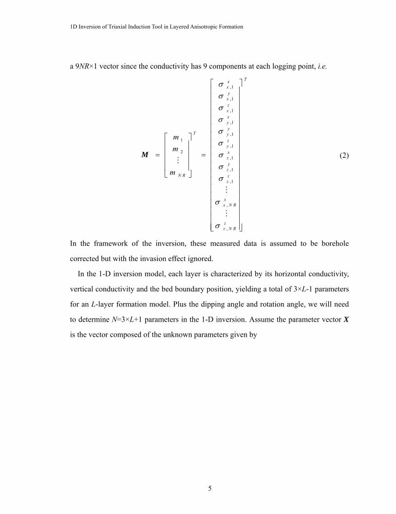
a 9NR×1 vector since the conductivity has 9 components at each logging point, i.e.
,1
,1
,1
,1
,11
,12
,1
,1
,1
,
,
Txxy
xzxxyy
T yzyxzy
zN R z
z
xx N R
zz N R
mm
m
σσσσσσσσσ
σ
σ
⎡ ⎤⎢ ⎥⎢ ⎥⎢ ⎥⎢ ⎥⎢ ⎥⎢ ⎥⎢ ⎥⎡ ⎤⎢ ⎥⎢ ⎥⎢ ⎥⎢ ⎥= = ⎢ ⎥⎢ ⎥⎢ ⎥⎢ ⎥⎢ ⎥⎣ ⎦⎢ ⎥⎢ ⎥⎢ ⎥⎢ ⎥⎢ ⎥⎢ ⎥⎢ ⎥⎣ ⎦
M (2)
In the framework of the inversion, these measured data is assumed to be borehole
corrected but with the invasion effect ignored.
In the 1-D inversion model, each layer is characterized by its horizontal conductivity,
vertical conductivity and the bed boundary position, yielding a total of 3×L-1 parameters
for an L-layer formation model. Plus the dipping angle and rotation angle, we will need
to determine N=3×L+1 parameters in the 1-D inversion. Assume the parameter vector X
is the vector composed of the unknown parameters given by

1D Inversion of Triaxial Induction Tool in Layered Anisotropic Formation
6
1
1
/32
,1
,1
, /3
, /3
log( )log( )log( )
log( )log( )log( )
log( )log( )
T
T
L
h
vN
h L
v L
Zx
ZxX
x
αγ
σσ
σσ
⎡ ⎤⎢ ⎥⎢ ⎥⎢ ⎥⎢ ⎥
⎡ ⎤ ⎢ ⎥⎢ ⎥ ⎢ ⎥⎢ ⎥ ⎢ ⎥= =⎢ ⎥ ⎢ ⎥⎢ ⎥ ⎢ ⎥⎣ ⎦ ⎢ ⎥
⎢ ⎥⎢ ⎥⎢ ⎥⎢ ⎥⎣ ⎦
(3)
All parameters within the proper magnitude range are rescaled due to the application
of logarithm. Then we use the parameter vector X to construct the following objective
function (cost function) 1( ) ( ) ( )2
= TC X R X R X (4)
where R(X) is the residual function defined by ( ) ( )= −R X S X M , ( )S X is the
simulated tool response corresponding to a particular model in terms of the vector X.
As we can see, the cost function measures the error between the calculated log and the
input log. The smaller the cost function is, the more reliable inversion results we may
obtain. Hence the most critical procedure in the inversion is to reduce the cost function.
We choose the classical nonlinear inversion approach, Gauss-Newton minimization
algorithm in our 1-D inversion. According to Taylor expansion, we can approximate the
cost function C(X) with a local quadratic model as follows [12] 1 1( ) ( ) ( ) ( )( ( ( )(2 2
≈ + +T T Tc c c c c c cC X R X R X g X X-X ) X-X ) H X X-X ) (5)
where ( ) ( ) ( ) ( )=∇ = Tg X C X J X R X is the gradient of the cost function C(X) and
( ) ( )=∇∇H X C X is the Hessian of the cost function C(X) which is given by

1D Inversion of Triaxial Induction Tool in Layered Anisotropic Formation
7
( ) ( ) ( ) ( ) ( ) ( ) μ= + ≈ +T TH X J X J X S X J X J X I . (6)
where 9
2
1( ) ( ) ( )
×
=
= ∇∑NR
i ii
S X r X r X denotes the second-order information in ( )H X . In (6),
we apply the Cholesky factorization algorithm to update μ . By determining 0μ > ,
( ) ( ) ( ) μ≈ +TH X J X J X I is positive definite, which guarantees the minimum of the cost
function to be found. Then (5) can be rewritten as 1 1( ) ( ) ( ) ( ) ( )( ) ( ) ( ( ) ( ) )( )2 2
μ≈ + − + − + −T T T Tc c c c c c c c cC X R X R X R X J X X X X X J X J X I X X (7)
Then the solution of (7) is given by
1( ( ) ( ) ) ( ) ( )μ −+ ≈ − +T T
c c c c cX X J X J X I J X R X (8)
The details of the Cholesky factorization algorithm can be referred to [13] and is omitted
here.
2) Line Search Technique
Equation (8) provides us the Newton direction +≈ − cP X X . Usually this step can not
guarantee the minimum value of the cost function because of the poor match between the
cost function and the quadratic form. Therefore, we incorporate a line search along the
Gauss-Newton direction to guarantee a reduced cost function in each iteration until the
cost function satisfies:
1( ) ( )λ αλ δ ++ ≤ +k k k k kC X P C X C (9)
where { }0,1α ∈ , kλ is the kth line search step. In practice, α is a very small value
and we choose 410α −= in this paper. Starting from 1 κλ+ = +k k kX X P , the cost function C(X)
can be expressed as a quadratic form of the step length λ
22( ) ( ) a b cλ λ λ λ= + ≈ + +k kC C X P (10)

1D Inversion of Triaxial Induction Tool in Layered Anisotropic Formation
8
where a, b and c are constants determined from the current cost function C(λ),
( 0) ( )a λ= = = kC C X (11)
0
( ) ( )bλ
λλ =
= = Tk k
dC g X pd
(12)
{ }( ) ( )
12( )
1 ( ) ( )c λ λ δλ
+⎡ ⎤= + − −⎣ ⎦m m
k k k k k kmk
C X P C X C (13)
Thus, ( 1)mkλ
+ , which is the minimum of C(λ), for m=0, 1, 2….. is given by
{ }2( )1( 1)
( ) ( )12 2 ( ) ( )
mk km
k m mk k k k k k
bc
λ δλ
λ λ δ++
+
= − =⎡ ⎤+ − −⎣ ⎦
C
C X P C X C (14)
Then, we start with (0) 1λ =k and proceed with the backtracking procedure of (10) until (9)
is satisfied. In order to take advantage of the newly acquired information of the cost
function beyond the first backtrack and improve the accuracy, we replace the quadratic
model of Equation (10) with the following cubic form
2 32( ) ( ) a b c dλ λ λ λ λ= + ≈ + +k kC C X P + (15)
where
2 22 21 2 2 1
2 21 12 1 2 1
( ) (x )/ /1( ) (x )1/ 1/
k
k
C b CcC b Cdλ λλ λ λ λλ λλ λ λ λ
− −⎡ ⎤− ⎡ ⎤⎡ ⎤= ⎢ ⎥ ⎢ ⎥⎢ ⎥ − −− −⎣ ⎦ ⎣ ⎦⎣ ⎦
i (16)
1 2,λ λ are two previous subsequent search steps. Then the final solution to ( 1)mkλ
+ is given
by
2( 1) 3
3k
m c c dbd
λ + − + −= (17)
3) The Jacobian Matrix
In (8), the Jacobian matrix is given by

1D Inversion of Triaxial Induction Tool in Layered Anisotropic Formation
9
1 1 1 1
1
9 1 9 9
/ / /
( ) / / /
/ / /
i N
j j i j N
NR NR i NR N
s x s x s x
s x s x s x
s x s x s x× × ×
∂ ∂ ∂ ∂ ∂ ∂⎡ ⎤⎢ ⎥⎢ ⎥⎢ ⎥= ∂ ∂ ∂ ∂ ∂ ∂⎢ ⎥⎢ ⎥⎢ ⎥∂ ∂ ∂ ∂ ∂ ∂⎣ ⎦
J X (18)
Every entry of the Jacobian matrix can be estimated through a finite-difference
computation,
[ ]( ) (1 ) ( )j j i j i
i i
s x s x s xx x
∂ +Δ −≈
∂ Δ (19)
In our implementation, Δ is chosen to be 410− . The computation of the Jacobian
matrix is the most time-consuming part in the entire inversion procedure since in each
Gauss-Newton step we need to solve 9 NR N× × forward problems to construct the
Jacobian matrix.
4) The Constrain Algorithm
For better efficiency, it is necessary to impose a priori maximum and minimum bounds
for the unknown parameters. For this purpose, we introduce a nonlinear transformation
given by max min max min
x sin( )2 2
i i i ii i
x x x x c+ −= + , - <ci∞ <+∞ (20)
where max min,i ix x are the upper and lower bounds on the physical model parameter ix . It is
clear that
min , sin( ) 1i i ix x as c→ →− (21)
max, sin( ) 1i i ix x as c→ →+ (22)
Theoretically, by using this nonlinear transformation we should update the artificial
unknown parameters ic instead of the physical model parameters ix . However, it is
1D Inversion of Triaxial Induction Tool in Layered Anisotropic Formation
10
straightforward to show that
max min( )( )j j jii i i i
j j i i
s s sdx x x x xc xc x x∂ ∂ ∂
= = − −∂ ∂ ∂
(23)
The two successive iterates , 1i kx + and ,i kx of ix are related by
max min max min
, 1 , 1
max min max min
, ,
x sin( )2 2
sin( )2 2
i i i ii k i k
i i i ii k i k
x x x x c
x x x x c q
+ +
+ −= +
+ −= + +
(24)
where
max min,
max min
2c arcsin( )i k i i
ii i
x x xx x− −
=−
(25)
and , , 1 ,i k i k i kq c c+= − is the Gauss-Newton search step in ic towards the minimum of the
cost functional in (10). This Gauss-Newton direction in ix is related to the
Gauss-Newton direction in ic through the following relation
p ii i
i
dxqdc
= (26)
Therefore, by applying the relationship in (26) to (24), we obtain the following
relationship between the two successive iterates , 1i kx + and ,i kx of ix (the step-length kγ
along the search direction ix is assumed to be adjustable):
max min max min, ,
, 1 ,x cos sin2 2
k i k k i ki i i ii k i k k
k k
p px x x xxν ν
γγ γ+
⎛ ⎞ ⎛ ⎞⎛ ⎞+ += + − +⎜ ⎟ ⎜ ⎟⎜ ⎟
⎝ ⎠ ⎝ ⎠ ⎝ ⎠ (27)
where
max min, ,( )( )k i i k i k ix x x xγ = − − (28)
Thus, in the inversion process there is no need to compute either ic or iq explicitly.
This will reduce the round-off errors caused by the introduction of the nonlinear function.
1D Inversion of Triaxial Induction Tool in Layered Anisotropic Formation
11
5) Zero-D Inversion
Next, we will describe the choice of the initial model in the inversion procedure since
good initial model can significantly improve the efficiency of the inversion. In practical,
we do not know the exact number of the layers, therefore we employ a whole space
inversion (also called Zero-D inversion) to get the initial model. Zero-D inversion is
receiving increasing interest in the study of inversion [14]. The biggest difference
between Zero-D inversion and 1-D inversion is that Zero-D inversion inverts parameters
based on each logging point. In Zero-D inversion, at each logging point, we should invert
four parameters (the dipping angle, rotation angle, horizontal conductivity and vertical
conductivity). In order to be distinguished from the 1-D inversion, the initial guess of the
Zero-D inversion is called as starting values. Next, we will explain the choice of the
starting values in the zero-D inversion.
Starting Values
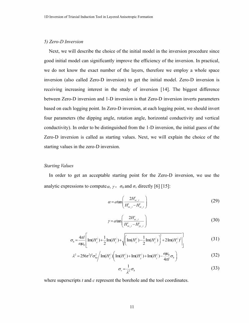
In order to get an acceptable starting point for the Zero-D inversion, we use the
analytic expressions to compute , α γ,σh and σv directly [6] [15]:
_
_ _
2tan
txz i
t txx i zz i
Ha
H Hα
⎛ ⎞= ⎜ ⎟⎜ ⎟−⎝ ⎠
(29)
_
_ _
2tan
cxy i
c cxx i yy i
Ha
H Hγ
⎛ ⎞= ⎜ ⎟⎜ ⎟−⎝ ⎠
(30)
' ' ' ' '
' ' ' ' '
22
0
4 1 1Im( ) Im( ) Im( ) Im( ) 2Im( )2 2
x z x z xh x z x z z
l H H H H Hπσωμ
⎡ ⎤⎛ ⎞⎢ ⎥= + + − +⎜ ⎟⎢ ⎥⎝ ⎠⎣ ⎦
(31)
' ' ' '
' ' ' '2 2 2 2 0256 Im( ) Im( ) Im( ) Im( )
4z x y z
ha hz x y zl H H H H
lωμλ π σ σπ
⎛ ⎞= + + −⎜ ⎟⎝ ⎠
(32)
2
1v hσ σ
λ= (33)
where superscripts t and c represent the borehole and the tool coordinates.

1D Inversion of Triaxial Induction Tool in Layered Anisotropic Formation
12
With the aid of the Zero-D inversion, the average values of α, γ are assumed as the initial
dipping and rotation angle.
Initial Boundary
After the initial dipping and rotation angle are determined, we need to determine the
initial boundary. We employ two methods together to determine the initial boundary:
(1) Variance based method of 2 v hσ σ−
(2) Horn effect of the cross components ,xz zxσ σ
The disadvantage of the first method is its instability. As we know, Zero-D inversion
results sometimes have large error. In this case, we can not completely rely on the
variance based method. As a good supplement, we use the horn effect of the cross
components ,xz zxσ σ to determine boundary since ,xz zxσ σ have obvious horn effect
when crossing the boundary. By combining the two methods, we can assure that no
boundary is missed.
The next important issue is how to detect and merge the redundant initial boundaries
during the 1-D inversion. In this paper, we employ the golden section search to merge
redundant layers.
6) Noise Analysis
According to Anderson [16], we incorporate two types of noises: coherent noise and
incoherent noise to simulate borehole noise, which is the main source of the noise. For
coherent noise, since the triaxial array is assumed to be co-located, the borehole noise
will be correlated in all the measurements. In this case, all coils should have the same
noise level. On the other hand, if the x, y, and z coils are not co-located, or if the tool is
moving at an irregular speed, the noise will be incoherent. In order to simulate incoherent

1D Inversion of Triaxial Induction Tool in Layered Anisotropic Formation
13
noise, an array of different random numbers will be generated for each measure channel
and then scaled and added as above [16].
7) Flow Chart of the Inversion
Fig. 2 shows the flow chart of the 1-D inversion. One can load the initial guess either
from Zero-D inversion or from a predetermined initial files.
Fig 2. Flow chart of 1-D inversion
3. Examples
Based on the above theory, we develop an 1-D inversion code. In this section, we will
demonstrate the capability and robustness of the code by synthetic data and a field log
data. If without specific illustration, in all the examples, initial models are provided by
Y
Raw Log Data
Stop?
Inversion results
Line search
Forward model
Zero-D inversion
Calculate Jacobian Matrix
Initial files
Initial parameters
Constraints
N

1D Inversion of Triaxial Induction Tool in Layered Anisotropic Formation
14
Zero-D inversion. No priori information is required in our inversion procedure. The
conductivity σ, dipping angle α, rotation angle γ, and the bed-boundary parameters Zi are
enforced to be within the following range:
1 1
0 1 2
2 1
0.0005 50.0001 890.0001 180
(2 2)i i i
L L N
Z Z Z i LD Z ZZ Z D
σαγ
− +
− −
< << < °< < °
< < ≤ ≤ −< << <
It should be noted that limits on boundary are dynamic. Do and DN are the depth of the
first and last measured data, respectively. Hence each layer can shift maximum between
the adjacent boundaries. The examples were run on a 2-core 2.61 GHz, 1.87 GB PC.
Example 1
In the first example, the formation model is a simple three-layer anisotropic model, as
shown in Fig. 3. The formation is characterized by a high-resistivity pay zone surrounded
by two symmetric isotropic zones.
The synthetic data used in this example are sampled from 10 ft to 50 ft with a 0.25 ft step.
We use the triaxial array as shown in Fig 1 to collect data. The distance between the
transmitter and receiver is 40 inches. The working frequency is 20 KHz. In this example,
the dipping angle is 30° and the rotation angle is 60°.
We apply the full matrix as well as the diagonal terms of the apparent conductivity
tensor as the input log data, respectively. By comparing the inversion results from these
two input data, we want to investigate whether reducing input data can still guarantee the
accuracy of the 1-D inversion.

1D Inversion of Triaxial Induction Tool in Layered Anisotropic Formation
15
Fig 3. A three-layer anisotropic model
Validation I— raw data
We first apply the raw data without noise to do inversion. The initial guess is provided
by the Zero-D inversion with the full matrix. Fig. 4 shows the initial guess and inverted
conductivity profile. The maximum relative error of the inverted horizontal and vertical
conductivities is less than 0.1%.
Tabel 1 presents the initial guess and inversion results of the dipping angle, rotation
angle obtained from the full matrix and the diagonal terms, respectively. We can see that
the inversion results from the full matrix and the diagonal terms match well with the true
parameters except the rotation angle given by the diagonal terms is different from the
true value. The inverted rotation angle (120°) becomes the coangle of the true rotation
angle (60°), which is caused by the elimination of all the cross components.
In Fig.5, we compare the raw data and the calculated responses from the inverted
formations. As can be seen, the components , , , , and xx yy zz yz zyσ σ σ σ σ from the inverted
formation obtained both the full matrix and diagonal terms coincide with the raw data.
Since the inverted rotation angle from the diagonal terms is the coangle of the true value,
The cross components , , and xz xz yz zyσ σ σ σ obtained from the diagonal term inversion
model are exactly in the reverse direction of the raw log since the inverted rotation angle
σh = 0.05 S/m, σv = 0.025 S/m
σh = 1 S/m, σv = 1 S/m
σh = 1 S/m, σv = 1 S/m 26’
34’

1D Inversion of Triaxial Induction Tool in Layered Anisotropic Formation
16
is the coangle of the true one. Thus we can conclude that neglecting the cross
components in inversion will introduce uncertainty when determining the rotation angle.
Table 2 shows the total CPU time cost by the inversions using the full conductivity
matrix and the diagonal terms, respectively. We can see that the when using the full
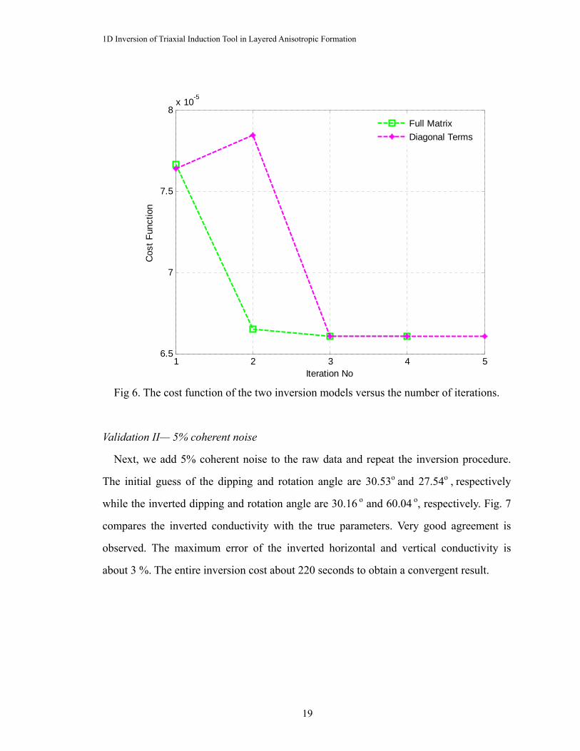
matrix to do the inversion, the procedure converges faster and cost less time. In Fig 6 we
compare the cost functions of the two inversion models versus the iteration numbers.
Compared with the full-matrix model, the diagonal-term model requires more iteration to
converge although each iteration cost less computation time, yielding slower behavior
than the full-matrix model. Due to the slower behavior and the uncertain effect on the
rotation angle of the diagonal-term model, we prefer to do the inversion using the full
conductivity matrix.
Table 1. The inverted dipping angle and rotation angle Validation I
Validation I Initial Guess Full Matrix Diagonal Term
α(°) 32.29 30.00 30.00
γ(°) 34.63 60.00 120.00
Table 2. The CPU time cost in Validation I
Inversion model Full Matrix Diagonal Term
Time (s) 92 106

1D Inversion of Triaxial Induction Tool in Layered Anisotropic Formation
17
10 15 20 25 30 35 40 45 50-0.5
0
0.5
1
1.5
Depth (ft)
σh (o
hm-m
)True σh
Initial σhFull MatrixDiagnal terms
10 15 20 25 30 35 40 45 50-0.5
0
0.5
1
1.5
Depth (ft)
σv (o
hm-m
)
True σv
Initial σvFull MatrixDiagnal Terms
Fig 4. Inverted conductivity profile with the synthetic raw data for the model in Fig. 3.
The true dipping angle and rotation angle are 30° and 60°, respectively. The solid
black line represents true anisotropic resistivity. The initial guess is shown by the gray
dotted line. The green dashed line with square mark represents the inverted results using
the full resistivity matrix. The purple dashed line with star mark represents the inverted
result using the diagonal terms.

1D Inversion of Triaxial Induction Tool in Layered Anisotropic Formation
18
20 40-1
0
1
Depth (ft)
σaxx
(s/m
)
20 40-0.05
0
0.05
Depth (ft)
σaxy
(s/m
)
20 40-0.5
0
0.5
Depth (ft)
σaxz
(s/m
)
20 40-0.05
0
0.05
Depth (ft)
σayx
(s/m
)
20 40-1
0
1
Depth (ft)σ
ayy (s
/m)
20 40-1
0
1
Depth (ft)
σayz
(s/m
)
20 40-0.5
0
0.5
Depth (ft)
σazx
(s/m
)
20 40-1
0
1
Depth (ft)
σazy
(s/m
)
20 400
0.5
1
Depth (ft)
σazz
(s/m
)Raw data Full Matrix Diagnal Terms
Fig 5. Comparison of the apparent conductivity simulated from the two
inverted model and the raw data.
1D Inversion of Triaxial Induction Tool in Layered Anisotropic Formation
19
1 2 3 4 56.5
7
7.5
8x 10⁻⁵
Iteration No
Cos
t Fun
ctio
n
Full MatrixDiagonal Terms
Fig 6. The cost function of the two inversion models versus the number of iterations.
Validation II— 5% coherent noise
Next, we add 5% coherent noise to the raw data and repeat the inversion procedure.
The initial guess of the dipping and rotation angle are 30.53o and 27.54o , respectively
while the inverted dipping and rotation angle are 30.16 o and 60.04 o, respectively. Fig. 7
compares the inverted conductivity with the true parameters. Very good agreement is
observed. The maximum error of the inverted horizontal and vertical conductivity is
about 3 %. The entire inversion cost about 220 seconds to obtain a convergent result.

1D Inversion of Triaxial Induction Tool in Layered Anisotropic Formation
20
10 15 20 25 30 35 40 45 50-0.5
0
0.5
1
1.5
Depth (ft)
σh (o
hm-m
)
10 15 20 25 30 35 40 45 50-0.5
0
0.5
1
1.5
Depth (ft)
σv (o
hm-m
)
True σh
Initial σh
Full Matrix
True σv
Initial σv
Full Matrix
Fig 7. Inverted conductivity obtained from the synthetic data for the model in Fig. 3 with the
input log contaminated by 5% coherent noise.
Validation III— 5% incoherent noise
Next, we add 5% incoherent noise to the input log data and repeat the inversion. The
inverted dipping and rotation angle are 30.5 o and 59.33 o, respectively, with a relative
error of 1.7 % and 1.2 % respectively. Fig.8 presents the inveted horizontal and vertical
conductivities. The maximum relative error of the inverted horizontal and vertical
conductivities is about 8%. From Fig.8, we can see that the presence of the incoherent
noise cause a stronger negative impact on the Zero-D inversion than the coherent noise
and more layers are generated in the initial guess. However, the inversion still yields
satisfactory results despite the bad initial guess. It cost about 508 seconds to obtain the
final inversion result.

1D Inversion of Triaxial Induction Tool in Layered Anisotropic Formation
21
10 15 20 25 30 35 40 45 50-0.5
0
0.5
1
1.5
Depth (ft)
σh (o
hm-m
)
10 15 20 25 30 35 40 45 50-0.5
0
0.5
1
1.5
Depth (ft)
σv (o
hm-m
)True σh
Initial σhFull Matrix
True σv
Initial σvFull Matrix
Fig 8. Inverted conductivity obtained from the synthetic data for the model in Fig. 3 with the
input log contaminated by 5% incoherent noise.
Example 2
Next, we will further validate our inversion algorithm using the Oklahoma benchmark
model [17]. The formation has 23 layers. The distance between the transmitter and the
receiver is 20 inches and the operating frequency is 20 KHz. The dipping angle is 60°
and the rotation angle is 0°.
Fig. 9 shows the real conductivity and the inverted conductivity obtained from the
contaminated data with 5% coherent noise and 5% incoherent noise. Table 3 gives the
initial guess of the dipping angle, rotation angle and the inverted dipping and rotation
angle for each case. The initial guess is modified from the Zero-D inversion results when
applying the raw data. Although redundant initial layers are given, our inversion code

1D Inversion of Triaxial Induction Tool in Layered Anisotropic Formation
22
successfully converged and provides reliable inversion results in all the three cases.In
Fig.10 we show the convergence property of the three cases. It is observed that the cost
function with the 5% coherent noise is a slightly higher than the other two cases due to
the misfit between the eighth and ninth layer. The inversion with 5% incoherent noise
consumes the most time. For this multilayer model, the inversion code took about 590,
491 and 650 minutes to obtain the final result under the three cases: uncontaminated raw
data, 5% coherent noise and 5% incoherent noise. It is found that the third case cost the
most time. Furthermore, we can see from Fig. 9 that the error becomes larger for high
resistive layers (the resistivity is larger than 100 ohm-m). This is reasonable since the
induction logging tool has a better sensitivity to the conductive layer than the resistive
layer. When the formation resistivity is larger than 100 ohm-m, the resolution of the
induction logging tool significantly decreased.
0 20 40 60 80 100 120 14010-4
10-2
100
102
Depth (ft)
σh (o
hm-m
)
0 20 40 60 80 100 120 14010-4
10-2
100
102
Depth (ft)
σv (o
hm-m
)
True σv
Initial σv
Raw Full Matrix5% Coherent Noise5% Incoherent Noise
Fig 9. Inverted conductivity with the synthetic raw data for the Oklahoma benchmark model.

1D Inversion of Triaxial Induction Tool in Layered Anisotropic Formation
23
Table.3 Inverted dipping angle, rotation angle with different input data
Initial Guess Raw Full Matrix Coherent Noise Incoherent Noise
α(°) 60.99 59.99 59.93 59.95
γ(°) 0.005 0.005 0.005 0.005
1 2 3 4 5 6 7 8 9 10 11 12 130
0.5
1
1.5
2
2.5
3x 10⁻³
Iteration No
Cos
t Fun
ctio
n
Full Matrix5% coherent5% incoherent
Fig 10. The cost functions versus the iteration number for the three inversion cases.
Example 3
As the final example, we apply the present inversion algorithm to an induction field
log taken from Well No 36-6, East Newkirk, Oklahoma [18], as shown in Fig. 11. The
induction tool is 6FF40. We use this example to investigate the capability of our 1-D

1D Inversion of Triaxial Induction Tool in Layered Anisotropic Formation
24
inversion model in the field exploration.
In Fig. 11, the solid line represents the field log from 6FF40. The dashed line
represents the inverted log from Ref. [18]. The polynomial expansion is used to fit the
field log and plot it in Fig. 12. Fig. 13 shows the inversion results from our 1-D inversion
code. For this example, we only need to invert the horizontal conductivity since it is
traditional induction logging. Both the dipping angle and rotation angle are 0°. In Fig. 14
we plot the calculated response from the inverted parameters and compare it with the
field log. By comparing Fig. 11 and Fig. 14, we can see that our calculated log is much
smoother compared with the inverted log from the published paper. In the beginning 20 ft,
our calculated log is much closer to the raw field data.
Fig 11. Field log measured by 6FF40 from Well No 36-6, East Newkirk, Oklahoma [19]. The
solid line represents the field log and the dashed line represents the inversion values in Ref. [18].

1D Inversion of Triaxial Induction Tool in Layered Anisotropic Formation
25
0 10 20 30 40 50 60 70 80 90100
101
102
Depth (ft)
Res
istiv
ity (o
hm-m
)
Fitted Field Log
Fig 12. Fitted field log as shown in Fig. 11

1D Inversion of Triaxial Induction Tool in Layered Anisotropic Formation
26
0 10 20 30 40 50 60 70 80 900
0.05
0.1
0.15
0.2
0.25
0.3
0.35
0.4
Depth (ft)
σh (S
/m)
Inversion results of fitted field log
Initial Guess1-D Inversion
Fig 13. Inverted resistivity of the fitted field log in Fig. 12 by applying the 1-D inversion
algorithm.

1D Inversion of Triaxial Induction Tool in Layered Anisotropic Formation
27
0 10 20 30 40 50 60 70 80 90100
101
102
Depth (ft)
Res
istiv
ity (o
hm-m
)
Fitted Field Log VS Calculated Log
Fitted Field LogCalculated Log
Fig 14. Comparison between the fitted field log from the Ref.[18] and the calculated log from the
inverted formation. The blue line is the fitted field log and the red line is the calculated log from
the 1-D inversion.
4. Summary
In this paper, we presented an inversion algorithm for triaxial induction logging in 1-D
layered transverse isotropic formation. The Gauss-Newton algorithm is employed to
modify Newton step from Gauss-Newton algorithm and thus reduces the cost function. In
order to improve the effectiveness of the Gauss-Newton algorithm, Gill and Murray
Cholesky factorization is used to calculate the Hessian matrix in the Quadratic model of
the cost function. Zero-D inversion is used to generate the initial guess. In order to obtain

1D Inversion of Triaxial Induction Tool in Layered Anisotropic Formation
28
good initial guess, both the variance-based method and the horn effect of the cross
components are used to determine the initial boundary. Then golden section search is
applied to merge redundant initial boundaries during the inversion. The resultant
inversion algorithm was validated by synthetic data from our forward modeling and other
different forward modeling. Satisfactory inversion results can be obtained in various
cases despite of the noise. We also demonstrate the capability of our code in the
application of the real field log inversion.

1D Inversion of Triaxial Induction Tool in Layered Anisotropic Formation
29
References
[1] C. J. Weiss and G. A. Newman, “Electromagnetic induction in a fully 3-D anisotropic
earth”, Geophysics, vol. 67, issue. 4, pp.1104–1114, July 2002.
[2] A. Abubakar, T. M. Habashy, V. Druskin, L. Knizhnerman, and S. Davydycheva, “A
3D parametric inversion algorithm for tri-axial induction data”, Geophysics, Vol. 71,
No. 1, pp. G1–G9, January 2006.
[3] A. B. Cheryauka and M. S. Zhdanov, “Fast modeling of a tensor induction logging
response in a horizontal well in inhomogeneous anisotropic formations”, SPWLA
42nd Annual Logging Symposium, June 2001.
[4] L. Yu, B. Kriegshauser, O. Fanini, and J. Xiao, “A fast inversion method for
multicomponent induction log data”, 71st Annual International Meeting, SEG,
Expanded Abstracts, pp. 361–364, 2001
[5] X. Lu, and D.Alumbaugh, “One-dimensional inversion of three component induction
logging in anisotropic media”, 71st Annual International Meeting, SEG, Expanded
Abstracts, pp. 376–380, 2001.
[6] Z. Zhang, L. Yu, B. Kriegshauser, and L. Tabarovsky, “Determination of relative
angles and anisotropic resistivity using multicomponent induction logging data”,
Geophysics, vol. 69, 898–908, July 2004.
[7] H. Wang, T. Barber, R. Rosthal, J. Tabanou, B. Anderson, and T. M. Habashy, “Fast
and rigorous inversion of triaxial induction logging data to determine formation
resistivity anisotropy, bed boundary position, relative dip and azimuth angles”, 73rd
Annual International Meeting, SEG, Expanded Abstracts, pp. 514–517, 2003.
[8] A. Abubakar, P. M. van den Berg, and S.Y. Semenov, “Two- and three-dimensional
algorithms for microwave imaging and inverse scattering,” Journal of
Electromagnetic Waves and Applications, vol.17, pp. 209-231, 2003.

1D Inversion of Triaxial Induction Tool in Layered Anisotropic Formation
30
[9] Davydycheva, V. Druskin, and T. M. Habashy, “An efficient finite-difference
scheme for electromagnetic logging in 3D anisotropic inhomogeneous media,”
Geophysics, vol. 68, pp. 1525–1536, September 2003.
[10] T. M. abashy, and A. Abubakar, “A general framework for constraint minimization
for the inversion of electromagnetic measurements,” Progress in Electromagnetic
Research, vol. 46, pp. 265-312, 2004.
[11] L. L. Zhong, J. Ling, A. Bhardwaj, S. C. Liang and R. C. Liu, “Computation of
Triaxial Induction Logging Tools in Layered Anisotropic Dipping Formations,”
IEEE Trans. Geosci. Remote Sens., vol.46, no.4, pp. 1148–1163, March 2008.
[12] J. E. Dennis, Jr. and R. B. Schnabel, “Numerical Methods for Unconstrained
Optimization and Nonlinear Equations”, in Prentice Hall series in computational
mathematics, 1983, pp.1-378.
[13] P. E. Gill and W. Murray, “Newton-type methods for unconstrained and linearly
constrained optimization,” Mathematical Programming, no. 28, pp.311-350, July
1974.
[14] P. Wu, G. L. Wang, and T. Barber, “Efficient Hierarchical Processing and
Interpretation of Triaxial Induction Data in Formations With Changing Dip,” SPE
Annual Technical Conference and Exhibition, September 2010
[15] M. Zhdanov, D. Kennedy, and E. Peksen, “Foundations of tensor induction
well-logging”, Petrophysics, vol. 42, pp. 588-610, 2001.
[16] B. I. Anderson, T. D. Barber, and T. M. Habashy, “The interpretation and inversion
of fully triaxial induction data; a sensitivity study”, SPWLA 43rd Annual Logging
Symposium, 2002.
[17] R. Rosthal, T. Barber, S. Bonner, “Field test results of an experimental fully-triaxial
induction tool”, SPWLA 44th Annual Logging Symposium, 2003.
1D Inversion of Triaxial Induction Tool in Layered Anisotropic Formation
31
[18] B. I. Anderson, T. D. Barber, and T. M. Habashy, “The interpretation and inversion
of fully triaxial induction data; a sensitivity study”, SPWLA 43rd Annual Logging
Symposium, 2002.
[19] R. Freedman, and G. N. Ninerbo, “Maximum entropy inversion of induction-log
data”, SPE formation evaluation, June 1991.
[20] N. Yuan, X. Chun Nie and R. Liu, “Improvement of 1-D simulation codes for
induction, MWD and triaxial tools in Multi-layered dipping beds”, Well Logging
Laboratory Technical Report, pp.32-71, October 2010.
[21] M. J. Wilt, D. L. Alumbaugh, H. F. Morrison, A. Becker, K. H. Lee, and M.
Deszcz-Pan, “Crosswell electromagnetic tomography: System design considerations
and field results”, Geophysics, vol. 60,no. 871-885, May 1995.
[22] Wang, and L. C. Shen, “IND2D users’ guide”, Well Logging Laboratory Technical
Report, pp.32-71, 1996.
[23] Y. Zhang, L. C. Shen, and C. Liu, “Inversion of induction logs based on maximum
flatness, maximum oil, and minimum oil algorithms”, Geophysics, vol. 59, no.9, pp.
1320-1326, September 1994.

Parallelization of Forward Modeling Codes using OpenMP
32
CHAPTER 2
Parallelization of Forward Modeling Codes using OpenMP
Abstract
Efficiency of a forward modeling code is very important for both efficient evaluation
of tool responses and log data interpretation in real time/post processing. With the
advancement of various high performance computing techniques such as Message
Passing Interface (MPI), Open Multi-Processing (OpenMP). OpenMP and computer
hardware technology such as graphics processing units (GPU), it is possible to
significantly improve the efficiency of the forward modeling by using these techniques.
In this paper, we apply OpenMP to parallelize several previously developed codes: 1. The
simulation codes for wireline induction and LWD triaxial tools in one-dimensional (1-D)
multilayered anisotropic formation 2. The three-dimensional (3-D) simulation code for
triaxial induction logging tools in arbitrarily anisotropic formations. The parallel process
is explained in detail and numerical examples are presented to demonstrate the capability
of the parallel codes. Comparison of the original code and the parallel code shows that
the latter is much faster without loss of accuracy. Then the codes are used to do some
investigations about directional electromagnetic (EM) propagation measurements.
1. Introduction
Efficiency of a computing code is always an important issue for users. In well logging
area, on one hand, an efficient forward modeling code can simulate the tool responses
fast and save CPU time for users. On the other hand, since the inversion process requires
a repeated computation of the forward modeling, efficient forward modeling is crucial to
faithful interpretation of log data acquired. Nowadays, the development of high
performance computing techniques provides us various choices to improve the speed of
the forward modeling without loss of accuracy. A graphics processing unit or GPU is a
specialized circuit designed to rapidly manipulate and alter memory in such a way so as
to accelerate the building of images in a frame buffer intended for output to a display.

Parallelization of Forward Modeling Codes using OpenMP
33
Modern GPUs are very efficient at manipulating computer graphics, and their highly
parallel structure makes them more effective than general-purpose CPUs for algorithms
where processing of large blocks of data is done in parallel. The most popular CPU-based
parallel techniques are Message Passing Interface (MPI) and Open Multi-Processing
(OpenMP). MPI was first implemented in 1992 [1] and remains the dominant method
used in high-performance computing today [2-4]. MPI is language-independent and can
be run on either symmetric multiprocessor (SMP), distributed shared memory (DSM)
processor or clusters, and supercomputers. However, MPI is relatively difficult to
implement in programming. On the contrary, the latest developed OpenMP is easy to
implement and therefore becomes an appropriate choice for less complicated algorithms.
OpenMP is an application programming interface that supports multi-platform shared
memory multiprocessing programming in Fortran, C, and C++ [5-8]. In this paper, we
apply OpenMP to parallelize the following forward modeling codes: 1. the forward
modeling code for wireline induction and LWD triaxial tools in 1-D layered anisotropic
formation; 2. the simulation code for induction triaxial logging tools in three-dimensional
(3-D) arbitrarily anisotropic formation. The principals of the forward modeling are briefly
explained and the parallel implementation of the codes is described in details. In the
numerical result section, we compare the total CPU time as well as the simulation results
of several examples between the original code and the parallelized code. After
parallelization, the computation speed is significantly on a multi-core computer and the
speed can be further improved as the number of the processor cores increases. The codes
are also used to do some interesting investigations and discussions will be presented in
the numerical result section.
2. Theory
2.1 Parallelization of the 1-D Simulation Codes for Wireline Induction and LWD
Triaxial Tools in Anisotropic Formations

Parallelization of Forward Modeling Codes using OpenMP
34
In this section, we will explain how to use OpenMP to parallel the simulation code for
wireline or LWD triaxial tools in 1-D layered anisotropic formation. This section is
arranged as follows. First, for the completeness of the paper, we briefly present the theory
on which the forward modeling of wireline and LWD triaxial logging is based. Then, we
will explain the parallel implementation of the codes using OpenMP for the 1-D Fortran
codes.
A. Forward Modeling of Wireline/LWD Triaxial Logging
Triaxial tool is an emerging logging tool to detect formation anisotropy and delineate
low resistivity reservoirs. A triaxial tool usually comprises one coaxial transmitter-
receiver pair and two coplanar transmitter-receiver pairs [9-15]. The transmitter/receiver
coils are perpendicular to each other. The formation anisotropy responds to different
components in tool transmitter–receiver combinations, thus providing additional
information for better formation evaluation. Our 1-D simulation for the response of
triaxial tools in anisotropic formations is based on an analytical method which solves the
Maxwell’s equations in the presence of magnetic dipole excitation analytically (both the
transmitter and receivers are modeled as magnetic dipoles since they are infinitely small)
[16-18]. The generalized upward and downward reflection coefficients are obtained from
the equivalent transmission line theory [19].
Consider a triaxial tool which includes three orthogonal transmitters and three
orthogonal receivers oriented at x, y and z direction, respectively, as shown in Fig.1. The
coils are assumed to be sufficiently small and can be replaced by point magnetic dipoles
in the modeling. Thus, the magnetic source excitation of the triaxial tool can be expressed
as )(),,( rM δzyx MMM= . If the transmitter/receiver is oriented at arbitrary directions,
the magnetic dipole will be projected to the x, y, z direction first and follow the same
analysis procedure.
For each component of the transmitter moments yx MM , and zM , there are in
general three components of the induced field at each point in the medium. Thus there are

Parallelization of Forward Modeling Codes using OpenMP
35
nine field components at each receiver location. These field components can be expressed
by a matrix representation of a dyadic H as:
⎥⎥⎥⎥
⎦
⎤
⎢⎢⎢⎢
⎣
⎡
=
zzzyzx
yzyyyx
xzxyxx
HHH
HHH
HHH
H (2)
where the first subscript corresponds to the transmitter index and the second subscript
corresponds to the receiver index, i.e. ijH denotes the magnetic field received by the j-
directed receiver coil excited by the i-directed transmitter coil. Next, we will derive the
expressions for the nine magnetic field components in 1-D multiple layered transverse
isotropic formation. A sketch showing a general geometry of a multi-component
induction logging tool in a layered anisotropic formation is given in Fig.2.
X
Y
z
T
X
Y
L1
R1 L2
Y
X
R2Main receiver
Bucking coils
Transmitter
X
Y
z
T
X
Y
L1
R1 L2
Y
X
R2Main receiver
Bucking coils
TransmitterMT
x
MT
MTz
y
Fig.1. Basic structure of a triaxial tool and the equivalent dipole model

Parallelization of Forward Modeling Codes using OpenMP
36
x
Y
z
z1
z2
z3
zi
zi+1
zN
zN-1
ε 1h ,μ0 , σ 1h , σ 1v
Transmitter
Receiver
Bucking coils
ε1v ,
ε 2h ,μ0 , σ 2h , σ 2vε2v ,
ε 3h ,μ0 , σ 3h , σ 3vε3v ,
εNh ,μ0 , σ Nh , σ NvεNv ,
Fig. 2 A triaxial tool in a 1-D layered anisotropic formation
The electromagnetic fields in a homogeneous transverse isotropic medium satisfy the
following Maxwell’s equation:
ˆˆ ˆ( ) ( ) ( ) ( )iσ ωε σ ′∇ × = − =H r E r E r (3a)
( ) ( ) ( )si iωμ ωμ∇× = +E r H r M r . (3b)
A harmonic time dependence tie ω− is used and suppressed throughout the paper. The
complex conductivity tensor σ ′ is
0 0
ˆ 0 00 0
h
h
v
σ
σ σσ
⎡ ⎤′⎢ ⎥⎢ ⎥′′ =⎢ ⎥
′⎢ ⎥⎣ ⎦
(4)
where h h hiσ σ ωε′ = − and v v viσ σ ωε′ = − .
Parallelization of Forward Modeling Codes using OpenMP
37
First, we will solve the Maxwell’s equation (3a) and (3b) in homogeneous transverse
isotropic medium. Following the procedure in [20], we introduce the Hertz vector
potential π and scalar potential Φ to represent the electric and magnetic field:
1ˆ( ) hiωμσ σ π−′= ⋅∇×E r (5)
and
ˆ( )( ) ( )hv
i σ πωμσ πσ
′∇ ⋅ ⋅′= + ∇′
H r (6)
For a x-directed magnetic dipole ( ,0,0)TxM=M , the Hertz vector potential has both x
and y components, i.e.
ˆ ˆx zx zπ π π= + (7)
where
,4
vik sx
xM e
sπ
πλ= (8)
2 ,4
v hik s ik rx
zM x e ez z
s rπ λ
πρ⎛ ⎞
= −⎜ ⎟⎝ ⎠
(9)
where 2 /h vλ σ σ′ ′= is the anisotropy ratio. 2h hk iωμσ ′= is the complex wave number in
the horizontal direction and 2v vk iωμσ ′= is the complex wave number in the vertical
direction. The distance ρ, r and S are given by 22 yx +=ρ , 222 zyxr ++= , and
2222 zyxs λ++= , respectively.
For a y-directed magnetic dipole (0, ,0)TyM=M , the Hertz vector potential has both y
and z components and for a z-directed magnetic dipole (0,0, )TzM=M , the Hertz vector
potential has only z component.
Parallelization of Forward Modeling Codes using OpenMP
38
Substituting the expressions of the Hertz vector potential into Eq. (6), we can obtain all
the nine components of the magnetic field generated by a magnetic dipole
)(),,( rM δzyx MMM= in a homogeneous TI medium,
2 2 2 2 2
2 4 22
4 4
v hik s ik rh h h v h h h
xxk ik s k k x ik x ik r k xe eH
s s rπ λ πρ ρ ρ⎡ ⎤ ⎡− −
= + − −⎢ ⎥ ⎢⎣ ⎦ ⎣
( )2 22 2 2
4 2 3 4 5
12 3 3hh h hk xik x ik ik x x
r r r rρ
⎤+⎥− − + + −⎥⎦
(10)
2 2
2 2 2 4 3 4 52 2 3 3 ,
44
v hik s ik rh v h h h h h
yx xyk k ik k ik k ike e xyH H xy
s r r r rππρ ρ ρ ρ⎡ ⎤⎡ ⎤
= = − − − − − + + −⎢ ⎥⎢ ⎥⎣ ⎦ ⎣ ⎦
(11)
23 2
3 3 ,4
hik rh
zx xz hikeH H xz krr rπ
⎡ ⎤= = − + −⎢ ⎥⎣ ⎦
(12)
2 2 2 2 2
2 4 2
24 4
v hik s ik rh h h v h h h
yyk ik s k k y ik y ik r k ye eH
s s rπ λ πρ ρ ρ⎡ ⎤ ⎡− −
= + − −⎢ ⎥ ⎢⎣ ⎦ ⎣
( )2 22 2 2
4 2 3 4 5
12 3 3 ,hh h h
k yik y ik ik y yr r r rρ
⎤+⎥− − + + −⎥⎦
(13)
23 2
3 3 ,4
hik rh
zy yz hikeH H yz krr rπ
⎡ ⎤= = − + −⎢ ⎥⎣ ⎦
(14)
( )2 2 2 22
2 3 4
1 3 34
hik r hh hzz h
k zik ik ze zH kr r r r rπ
⎡ ⎤+⎢ ⎥= + − − +⎢ ⎥⎢ ⎥⎣ ⎦
(15)
By solving the Maxwell’s equation (3) in multi-layered TI medium, we can obtain the
magnetic field response of multi-component induction tools in the formation. For a z-
directed magnetic dipole (0,0, )TzM=M , the Hertz vector potential and the magnetic
field in the ith layer are given by

Parallelization of Forward Modeling Codes using OpenMP
39
000( )
4hi hi hiz z z ziz
zi i ihi
Me F e G e J dξ ξ ξβ
π α αρ απ ξ
∞ − − −⎛ ⎞= + +⎜ ⎟
⎝ ⎠∫ (16)
)00 210
0
cos ( )4
hi hi hiz z z zizxzi hi i i
hi
z zMH e Fe G e J dz z
ξ ξ ξβφ ξ α αρ απ ξ
∞ − − −⎛ −= + −⎜ −⎝
∫ (17)
)00 210
0
sin ( )4
hi hi hiz z z zizyzi hi i i
hi
z zMH e Fe G e J dz z
ξ ξ ξβφ ξ α αρ απ ξ
∞ − − −⎛ −= + −⎜ −⎝
∫ (18)
0 300
= ( )4
hi hi hiz z z zizzzi i i
hi
MH e Fe G e J dξ ξ ξβ α αρ απ ξ
∞ − − −⎛ ⎞+ +⎜ ⎟
⎝ ⎠∫ (19)
where )(xJ n is the nth order Bessel function, and
( ) ,2/122hihi k−= αξ
1, if is in the th layer0, if is not in the th layer
zi
z
M iM i
β⎧
= ⎨⎩
The term with zhie ξ− represents the wave traveling in the +z direction and the term with zhie ξ+ represents the wave traveling in the –z direction. The ± sign is chosen to assure the
fields decay as z increases.
The generalized upward and downward reflection coefficients iF and iG can be derived
by enforcing the boundary conditions at the horizontal boundary iz z= based on the
equivalent transmission line theory [16-18]. The detailed derivation and expression are
omitted here.
For a x-directed magnetic dipole ( ,0,0)TxM=M , the Hertz vector potential and the
magnetic field in the ith layer are given by
000 ( )
4vi i vi i vi iz z z zx i
xi i ii vi
Me Pe Q e J dξ λ ξ λ ξ λβ
π α αρ απλ ξ
− −∞ −⎛ ⎞= + +∫ ⎜ ⎟
⎝ ⎠ (20)
( ) 10cos ( )4
hi hi vi i vi iz z z zxzi i i vi i vi i
MS e T e Pe Q e J dξ ξ ξ λ ξ λπ φ ξ ξ αρ α
π∞ − −= + − +∫

Parallelization of Forward Modeling Codes using OpenMP
40
( )0 0 010
0
cos ( )4
hi vi iz z z zxi
z zMe e J d
z zξ ξ λφ β αρ α
π∞ − − − − −
+ −−∫ , (21)
After tedious derivation, we can obtain the expression for the magnetic field components:
0 02 2 2 2 20
2 2 2 20
( sin cos sin4
sin cos cos ) ( )
vi i hi vi i
vi i hi hi
z z z z zx i ixxi hi i hi hi
i vi i
z z zihi i hi i hi
i
M PH k e e k e
Qk e S e T e J d
ξ λ ξ ξ λ
ξ λ ξ ξ
βφ β φξ φ
π λ ξ λ
φ φξ φξ α αρ αλ
∞ − − − − −
−
= − +∫
+ − +
0 02 2 20
1
cos 2 (4
) ( )
vi i hi vi i vi i
hi hi
z z z z z zx ii vi i hi i i vi i i vi
vi
z zi hi i hi
Mk e e P k e Q k e
S e T e J d
ξ λ ξ ξ λ ξ λ
ξ ξ
βφ λ β ξ λ λ
πρ ξ
ξ ξ αρ α
∞ − − − − −
−
+ + + +∫
+ −
(22)
0 02 20
20
sin cos (4
) ( )
vi i hi vi i
vi i hi hi
z z z z zx i iyxi hi i hi hi
i vi i
z z zihi i hi i hi
i
M PH k e e k e
Qk e S e T e J d
ξ λ ξ ξ λ
ξ λ ξ ξ
βφ φ β ξ
π λ ξ λ
ξ ξ α αρ αλ
∞ − − − − −
−
= − − −∫
− − +
0 02 20
21
sin 2 (4
) ( )
vi i hi vi i
vi i hi hi
z z z z zx ii vi i hi i i vi
viz z z
i i vi i hi i hi
Mk e e P k e
Q k e S e T e J d
ξ λ ξ ξ λ
ξ λ ξ ξ
βφ λ β ξ λ
πρ ξ
λ ξ ξ αρ α
∞ − − − − −
−
+ + +∫
+ + − (23)
00 210
0
cos ( ) ( )4
hi hi hiz z z zxzxi i i i
z zMH e S e T e J d
z zξ ξ ξφ β α αρ α
π∞ − − −−
= + +∫− (24)
where
( )1/ 22 2vi vikξ α= −
The generalized upward and downward coefficients , ,i i iP Q S and iT can be obtained by
matching the boundary conditions at the interface of the ith and (i+1)th layer [16-18].
For a y-directed magnetic dipole (0, ,0)TyM=M , the Hertz vector potential and the
magnetic field in the ith layer are given by

Parallelization of Forward Modeling Codes using OpenMP
41
000( )
4vi i vi i vi iz zy z zi
yi i ii vi
Me Pe Q e J dξ λ ξ λ ξ λβπ α αρ α
πλ ξ∞ − − −⎛ ⎞
= + +⎜ ⎟⎝ ⎠
∫ (25)
( ) 10sin ( )
4hi hi vi i vi iy z z z z
zi i i vi i vi i
MS e T e Pe Q e J dξ ξ ξ λ ξ λπ φ ξ ξ αρ α
π∞ − −= + − +∫
( )0 0 010
0
sin ( )4
hii vi iz z z zyi
M z ze e J d
z zξ ξ λφ β αρ α
π∞ − − − − −
+ −−∫ (26)
0 02 20
20
sin cos (4
) ( )
vi i hi vi i
vi i hi hi
z z z zy zi ixyi hi i hi hi
i vi i
z z zihi i hi i hi
i
M PH k e e k e
Q k e S e T e J d
ξ λ ξ ξ λ
ξ λ ξ ξ
βφ φ β ξπ λ ξ λ
ξ ξ α αρ αλ
∞ − − − − −
−
= − − −
− − +
∫
0 02 20
21
sin 2 (4
) ( )
vi i hi vi i
vi i hi hi
z z z zy zi ii vi i hi hi
vi i
z z zihi i hi i hi
i
M Pk e e k e
Q k e S e T e J d
ξ λ ξ ξ λ
ξ λ ξ ξ
βφ λ β ξπρ ξ λ
ξ ξ αρ αλ
∞ − − − − −
−
+ + +
+ + −
∫ (27)
0 02 2 2 2 20
2 2 2 20
( cos sin cos4
cos sin sin ) ( )
vi i hi vi i
vi i hi hi
z z z zy zi iyyi hi i hi hi
i vi i
z z zihi i hi i hi
i
M PH k e e k e
Q k e S e T e J d
ξ λ ξ ξ λ
ξ λ ξ ξ
β φ β φξ φπ λ ξ λ
φ φξ φξ α αρ αλ
∞ − − − − −
−
= − +
+ − +
∫
0 02 20
21
cos 2 (4
) ( )
vi i hi vi i
vi i hi hi
z z z zy zii vi i hi i i vi
viz z z
i i vi i hi i hi
Mk e e P k e
Q k e S e T e J d
ξ λ ξ ξ λ
ξ λ ξ ξ
βφ λ β ξ λπρ ξ
λ ξ ξ αρ α
∞ − − − − −
−
+ − − −
− − +
∫ (28)
00 210
0
sin ( )4
hi hi hiz zy z zzyi i i i
M z zH e S e T e J d
z zξ ξ ξφ β α αρ α
π∞ − − −⎛ − ⎞
= + +∫ ⎜ ⎟−⎝ ⎠ (29)
Again, the generalized upward and downward reflection coefficients , ,i i iP Q S and iT
can be obtained by matching the boundary conditions at the interface of the ith and
(i+1)th layer [16-18].
In the present work, both the errors in the equations and the code for the Hertz potential
and magnetic fields in [16,17] are corrected.

Parallelization of Forward Modeling Codes using OpenMP
42
For convenience of explanation of the parallelization procedure, we plot the flow chart
of the forward modeling code in Fig.3. From the flow chart, we can see that the dominant
part of the computation including the calculation of the generalized upward and
downward reflection coefficients and the Hankel transforms of the highly oscillating
integrals of the Bessel functions is repeated for every logging point. This code is
programmed in serial and only one core is used even the code is run on a multi-core
computer. To fully explore the resources of the multi-core computer, we parallel the
forward modeling code using OpenMP.

Parallelization of Forward Modeling Codes using OpenMP
43
Fig. 3 Flow chart of the forward modeling code for simulation of triaxial tool responses
Start
Read tool and formation parameters
Calculate the effective dielectric constant and the converting table for the given tool
Loop for each pair of transmitter and receiver
Loop for each logging point
Sum of the above field and Convert to apparent resistivity
Output the magnetic field and apparent resistivity
End
Calculate the magnetic field in homogeneous media
Calculate the magnetic field in layered TI media (Hankel transform and reflection coefficients calculation)

Parallelization of Forward Modeling Codes using OpenMP
44
In the forward modeling code for LWD triaxial tools, we use the effective dielectric
constant in the tool response simulation and apparent resistivity/conductivity conversion.
We use the effective dielectric constant model shown in Table 1 for different service
companies.
Table 1 Dielectric Constant Model
Company Dielectric constant model APS Technology 0.42210r tRε −= × (for 2MHz)
0.49480 8r tRε −= × + (for 400KHz) Baker Hughes INTEQ 26.4 4.5255 1 1 (2275 / )r tRε = + + + (for
2MHZ) 26.4 4.5255 1 1 (11375 / )r tRε = + + + (for
400KHz) GE Energy 0.35108.5 5r tRε −= × + Halliburton Sperry-Sun 10rε = Pathfinder 0.35108.5 5r tRε −= × + (AWR)
10rε = (CWR) Schlumberger Anadrill 0.35108.5 5r tRε −= × + (for 2MHz)
0.46279.7 5r tRε −= × + (for 400KHz) Weatherford 0.42210r tRε −= × (for 2MHz)
0.49480 8r tRε −= × + (for 400KHz)
B. Parallelization of the 1-D Forward Modeling Codes
We choose OpenMP to improve the performance of the code, and at the same time,
keeping the clarity of the original serial code. Thus, OpenMP emerge as reliable
alternative as it is just a set of compiler directives with library routines for parallel
application that greatly simplifies writing multi-threaded programs. We choose Intel
Fortran as the complier since it supports the OpenMP interface. The main loop shown in
Fig.3 repeated for every logging point dominants the entire computation time. Since the
calculation for each logging point is completely independent with each other, we can

Parallelization of Forward Modeling Codes using OpenMP
45
threat the whole repeated calculation as a master thread and run the calculations for
different logging points through several slave threads. The number of threads is
determined by the number of computer cores. Consequently, more than one logging point
is computed simultaneously but just consuming a single point’s time. We apply
PARALLEL DO to realize the parallel implementation and the programming structure of
the parallel code is shown in Fig. 4. The basic directive of PARALLEL DO is
semantically equivalent to:
!$OMP PARALLEL DO
DO I = 1, Nlog
…..
END DO
$OMP END PARALLEL DO
Then we implement PARALLEL DO to realize parallelization, as shown in Fig. 5.
Fig. 4 Programming structure of parallel 1-D simulation codes for wireline/LWD triaxial tools
In the programming, we should pay attention to the common block/variables in the
code. Since OpenMP is based on a shared-memory structure, all the threads are allowed
Read tool and formation information
DO Loop
Response of Single Logging Point
Output
Depth_end
Depth_start?
PARALLEL

Parallelization of Forward Modeling Codes using OpenMP
46
to access the common block or variables. However, some common blocks are not
supposed to be shared among different threads. The command THREADPRIVATE
allows us to specify named common blocks and variables as private to other threads but
global within their own thread. Once we declare a common block or variable as
THREADPRIVATE, each thread in the team maintains a separate copy of that common
block or variable. Data written to a THREADPRIVATE common block or variable
remain private to that thread and is not available to other threads in the team. Use the
clause COPYIN after the directive PARALLEL DO to specify that upon entry into a
parallel region, data of a named common block or named variable in the master thread are
copied to the common block or variable of each thread. Fig. 5 shows the comparison of
the structure of the serial and the parallel codes. Assume the code need to calculate 1000
logging point on a 4-core computer. In the serial code, the computer handles one logging
point at one time with only one processor active. On the contrary, in the parallel code, the
computer divides all the 1000 points into 4 groups (we assume the division is even
without loss of generality). As a result, 4 threads synchronously run the calculation and
the total computation time is significantly reduced.
Fig. 5 Comparison of the structure of the serial code and the parallel code
Serial code
1 2 3 4 5
998 999 1000
1~250
751~1000
251~500
501~750
Thread 1
Thread 3
Thread 2
Thread 4 Parallel code

Parallelization of Forward Modeling Codes using OpenMP
47
2.2 Parallelization of the 3-D Simulation Code for Triaxial Tools in Arbitrarily
Anisotropic Formations
A. Forward Modeling of Triaxial Tools in 3-D Arbitrarily Anisotropic Formations
In this part, we will use the finite difference method (FDM) to simulate the response of
a triaxial tool in 3-D arbitrarily anisotropic formation. x
Yz
z1
z2
z3
zi
zi+1
zN
ε1 σ1 ,
ε2 σ2 ,
εΝ σΝ ,
Transmitter
Receiver
Bucking coils
Fig. 6 A triaxial tool in a 3-D arbitrarily anisotropic formation
Consider a triaxial tool in a 3-D formation as shown in Fig.6. The governing equations
for EM induction in the 3-D geometry are Faraday’s law and Ampere’s law
BE ωi−=×∇ (30a)
DJJH ωisi ++=×∇ (30b)
where sJ is the source current density and iJ is the induced current density. In the above
equations, a time-harmonic dependence of i te ω is assumed and suppressed. The induced
current density iJ is related to the electric field by
EJ σ=i (31)

Parallelization of Forward Modeling Codes using OpenMP
48
The total electric field E can be expressed as the sum of a primary field 0E from sJ
embedded in a background reference medium and a scattered field E ′ arising from the
conductivity and permittivity variations which deviate from the background medium. In
geophysical applications, we usually prefer a scattered-field formulation instead of a
total-field one since the former computations are more robust and accurate, particularly
when the measurements are made very close to the source. A total-field solution usually
requires very fine meshes, resulting in large demands of computational resources. In
addition, it is impossible to obtain accurate in-phase responses from the total-field
solution since the direct-coupled field is dominant in the total field.
Setting ′=E E in (30) and combining (30)-(31) yield a single, second order partial-
differential equation (PDE) in terms of the scattered electric field:
( ) 000 JEE ωμωεσωμ jii −=′++′×∇×∇ (32)
The term 0J is the effective source current density for the scattered fields,
( )( ) ( )( )[ ] 0000 EIrIrJ εεωσσ −+−= j (33)
where I is the 3×3 identity matrix. It is noted that both the conductivity and permittivity
are position-dependant and can be fully anisotropic, i.e.:
( )xx xy xz
yx yy yz
zx zy zz
σ σ σσ σ σ σ
σ σ σ
⎡ ⎤⎢ ⎥
= ⎢ ⎥⎢ ⎥⎣ ⎦
r , ( )xx xy xz
yx yy yz
zx zy zz
ε ε εε ε ε ε
ε ε ε
⎡ ⎤⎢ ⎥
= ⎢ ⎥⎢ ⎥⎣ ⎦
r (34)
Next, we use the finite-difference method based on the staggered Yee grid [21] to solve
(32). The solution domain is discretized into Cartesian cells and the scattered electric
field components xE , yE and zE are defined on the edges of the cells. The magnetic-
field component xH is staggered in y and z, yH in x and z, and zH in x and y, as shown in
Fig. 7.
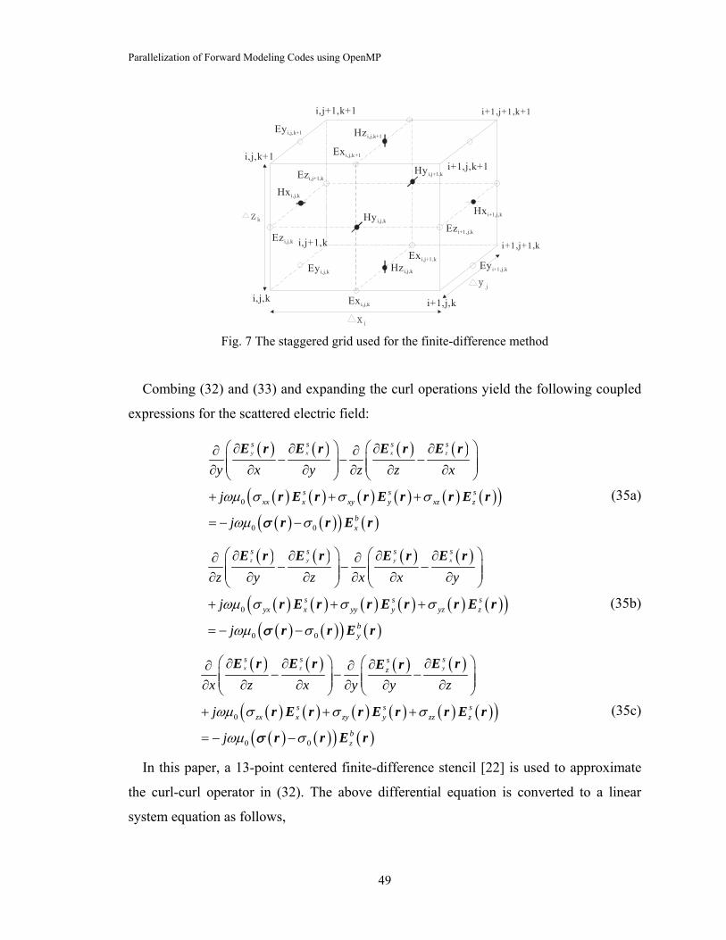
Parallelization of Forward Modeling Codes using OpenMP
49
zk
xi
yj
Eyi,j,k+1
Exi,j,k+1
Ezi,j,k
Eyi,j,k
i,j,k+1
Exi,j,k
Exi,j+1,kEyi+1,j,k
Ezi,j+1,k
Hxi,j,k
Hzi,j,k+1
Hyi,j,k
Hzi,j,k
Hyi,j+1,k
Hxi+1,j,k
Ezi+1,j,k
i+1,j+1,k
i+1,j+1,k+1
i,j,k
i,j+1,k+1
i+1,j,k
i+1,j,k+1
i,j+1,k
Fig. 7 The staggered grid used for the finite-difference method
Combing (32) and (33) and expanding the curl operations yield the following coupled
expressions for the scattered electric field:
( ) ( ) ( ) ( )
( ) ( ) ( ) ( ) ( ) ( )( )( ) ( )( ) ( )
0
0 0
y x x zs s s s
s s sxx x xy y xz z
bx
y x y z z x
j
j
ωμ σ σ σ
ωμ σ
⎛ ⎞ ⎛ ⎞∂ ∂ ∂ ∂∂ ∂− − −⎜ ⎟ ⎜ ⎟⎜ ⎟ ⎜ ⎟∂ ∂ ∂ ∂ ∂ ∂⎝ ⎠ ⎝ ⎠
+ + +
= − −
E r E r E r E r
r E r r E r r E r
r r E rσ
(35a)
( ) ( ) ( ) ( )
( ) ( ) ( ) ( ) ( ) ( )( )( ) ( )( ) ( )
0
0 0
z y y xs s s s
s s syx x yy y yz z
by
z y z x x y
j
j
ωμ σ σ σ
ωμ σ
⎛ ⎞ ⎛ ⎞∂ ∂ ∂ ∂∂ ∂− − −⎜ ⎟ ⎜ ⎟⎜ ⎟ ⎜ ⎟∂ ∂ ∂ ∂ ∂ ∂⎝ ⎠ ⎝ ⎠
+ + +
= − −
E r E r E r E r
r E r r E r r E r
r r E rσ
(35b)
( ) ( ) ( ) ( )
( ) ( ) ( ) ( ) ( ) ( )( )( ) ( )( ) ( )
0
0 0
x z ys s ss
z
s s szx x zy y zz z
bz
x z x y y z
j
j
ωμ σ σ σ
ωμ σ
⎛ ⎞ ⎛ ⎞∂ ∂ ∂∂∂ ∂− − −⎜ ⎟ ⎜ ⎟⎜ ⎟ ⎜ ⎟∂ ∂ ∂ ∂ ∂ ∂⎝ ⎠ ⎝ ⎠
+ + +
= − −
E r E r E rE r
r E r r E r r E r
r r E rσ
(35c)
In this paper, a 13-point centered finite-difference stencil [22] is used to approximate
the curl-curl operator in (32). The above differential equation is converted to a linear
system equation as follows,

Parallelization of Forward Modeling Codes using OpenMP
50
KE = S (36)
where the matrix K is the system matrix of dimension 3 3x y z x y zN N N N N N× for a
model with 3 x y zN N N cells. E is a vector of length 3 x y zN N N containing the secondary
electric filed values sxE , s
yE , szE for all nodes. S (length 3 x y zN N N ) is the secondary-
source vector given by the right-hand side of (35). The system matrix K is a sparse
matrix with up to 13 nonzero entries per line. The entries depend on the grid spacing and
the frequency-dependent properties of the media.
In the derivation of the linear equations, a conductivity averaging scheme is used to
obtain the conductivity at the center of the cell edge (where the electric field is defined).
Following the scheme in [22], the conductivity at the center of the edge is expressed as a
weighted sum of the conductivities of the four adjoining cells. The Dirichlet condition is
applied to the scattered electric field components on the outmost boundary of the finite-
difference mesh. The detailed expression of the matrices can be found in the Appendix. It
should be noted that the system equation is non-symmetric originally. By multiplying (A-
1) by Δxi+1/2ΔyjΔzk, (A-2) by ΔxiΔyj+1/2Δzk, and (A-3) by ΔxiΔyjΔzk+1/2, we can obtain the
symmetric form of the system equation, where Δxi, Δyj, Δzk are the length of grid cells i, j,
and k; Δxi+1/2, Δyj+1/2 and Δzk+1/2 are the distances between the centers of cells i+1 and i ,
j+1 and j , and k+1 and k, respectively.
The linear system in (36) is solved efficiently using a generalized minimal residual
(GMRES) algorithm [23] and the incomplete LU preconditioner (ILU) [24] is used to
improve the convergence of the matrix equation. Once the electric field is obtained from
equation (36), the magnetic field can be calculated from Faraday’s law.
Since the formation we considered is inhomogeneous and anisotropic, a fine mesh is
necessary to model the complicated structures and interfaces between different media.
However, a fine mesh yields large computer resource. A feasible way to alleviate this
difficulty is to use reasonably coarse mesh to model the geometry and use the averaged
conductivity for each cell to model the electrical property of the media. This is a good
compromise between accuracy and computational complexity. So in most cases, the grid

Parallelization of Forward Modeling Codes using OpenMP
51
used in the finite-difference method is independent on the electrical property of the
formation and different media can be included in a single rectangular cell by using the
averaged conductivity. In this paper, a technique similar to the one described in [22] is
used to calculate the average conductivity tensor. After a series of derivation, we can
write out the average conductivity entry xxσ as,
( )( )( ), ,1 1
10
1
y z
x
N Nx
Ni j kj k
xxi
xx xy z
N
J V xN N
σσ
′= =
′=
⎛ ⎞⎜ ⎟⎜ ⎟⎜ ⎟⎜ ⎟⎝ ⎠= Δ =
∑∑∑
(37)
Equation (37) implies that the averaged conductivity xxσ is obtained by first combining in series the xN subcells with the same superscript i in a line and then combining in parallel the yx NN × lines of subcells.
The average conductivity yxσ can be derived as,
( )
( )
( ), ,
( , , ) ( , , )1 1 1
10
1yx z
x
NN N i j kNyx i j k i j ki j k
xx xxi
yx yy z
J V xN N
σσ σ
σ
′= = =
′=
⎛ ⎞⎜ ⎟
∑ ∑ ∑ ⎜ ⎟∑⎜ ⎟
⎝ ⎠= Δ = (38)
The other average conductivity entries yyσ , zzσ , xzσ and yzσ can be derived out following a similar derivation procedure and written in a similar form. To preserve the symmetric character of the average conductivity tensor, we set the average conductivity entries αβσ to be the average of the calculated αβσ and βασ , that is
( ) βαβασσσσ βααββααβ ≠==+== ,, ,, 21 zyxzyx (39)
The details of the derivation are omitted and can be referred to Ref. [25].
Based on the above theory, we developed a forward modeling code to simulate the
responses of triaxial induction tools in 3-D arbitrarily anisotropic formation. Fig. 8 shows
the flow chart of the code. It is known that in the FDM, the mesh should be denser in the
vicinity of the tool in order to obtain good accuracy, and coarser in the region far away
from the tool to keep the overall grid size in a reasonable level. As can be seen in the
flow chart, there two options: 1) the mesh can be adjusted for different observation point;

Parallelization of Forward Modeling Codes using OpenMP
52
2) a fixed mesh is used for all observation points. If the mesh is adjusted according to the
observation points, the computation of the average conductivity tensor, the filling of the
matrix equation and the computation of the preconditioner must be repeated once the
mesh is changed. In this paper, we use a fixed mesh for all the observation points so that
the above time consuming computation is performed only once. This will yield some
scarification in the accuracy, particularly for points at the formation boundary.
Fortunately, via the use of the averaged conductivity technique mentioned previously, the
problem is greatly alleviated. Again, besides the calculation of the ILU preconditioner,
the most time consuming of the 3-D code is the repeated calculation for large number of
logging points. We use the OpenMP to parallel this part of the code. If users prefer an
adjustable mesh for different logging point, both the coefficient matrix and the
preconditioner matrix must be calculated repeatedly. Then this part also needs to be
implemented in parallel, as shown in Fig.8.

Parallelization of Forward Modeling Codes using OpenMP
53
Fig.8 The flow chart of the 3-D FDM forward modeling code
Implement in parallel for a fixed mesh
Implement in parallel for an adjustable mesh

Parallelization of Forward Modeling Codes using OpenMP
54
2. Numerical Results
In this section, we will present examples to demonstrate the performance of the
parallelized 1-D and 3-D forward modeling code respectively.
A). 1-D Forward Modeling Code
First, we compare the performance of the original serial 1-D forward modeling code
and the parallel code.
The first example is a 7-layer anisotropic model as shown in Fig.9. The parameters are
given in the figure. The dipping angle (the angle between the tool axis and the normal to
the layer boundaries) is 30o and the spacing between the transmitter and receiver is 1.8m.
L1
L2
L3
L4
L5
L6
L7
R =1 -m, R =10 -mh vΩ Ω
R =1 -m, R =10 -mh vΩ Ω
R =1 -m, R =10 -mh vΩ Ω
R=80 -mΩ
R=10 -mΩ
R=0.3 -mΩ
R =1 -m, R =10 -mh vΩ Ω
z
xy
o
α
0m
1.6m
3.8m
7.75m
8.75m
Dep
th(m
)
6.0m
Fig. 9 A Seven-layer anisotropic model
Fig. 10 shows the magnetic field responses at 25KHz, 50KHz and 100KHz obtained
from the serial code and the parallel code. We can see that the results from the two codes
coincide perfectly with each other, implying that the parallelization does not introduce
any error. Fig. 11 shows the computation time of the two codes as a function of the
number of logging points. It can be seen that as the number of logging points increases,
the total CPU time of both codes increase. But the increase of the parallel code is much
slower than that of the serial code. For the same number of logging point, the parallel

Parallelization of Forward Modeling Codes using OpenMP
55
code cost only 1/3 time that of the serial code when the code is run on a 4-core 2.33GHz
PC.
0 2 4 6 8 10-0.006
-0.004
-0.002
0.000
0.002
0.004
0.006
0.008
0.010
0.012
Im(H
xx) (
A/m
)
Depth(m)
25KHz,serial code 50KHz,serial code 100KHz,serial code 25KHz,parallel code 50KHz,parallel code 100KHz,parallel code
(a) Hxx
0 2 4 6 8 10-0.008
-0.006
-0.004
-0.002
0.000
0.002
0.004
0.006
0.008
Im(H
yy) (
A/m
)
Depth (m)
25KHz,serial code 50KHz,serial code 100KHz,serial code 25KHz,parallel code 50KHz,parallel code 100KHz,parallel code
(b) Hyy

Parallelization of Forward Modeling Codes using OpenMP
56
0 2 4 6 8 10-0.020
-0.015
-0.010
-0.005
0.000
Im(H
zz) (
A/m
)
Depth (m)
25KHz, serial code 50KHz, serial code 100KHz, serial code 25KHz, parallel code 50KHz, parallel code 100KHz, parallel code
(b) Hzz
Fig.10 The magnetic field response of the 7-layer model obtained from the serial code and the parallel code
0 1000 2000 3000 4000 5000
0
50
100
150
200
250
300
CPU
tim
e (S
econ
ds)
Number of logging points
Serial code Parallel code
Fig. 11 The CPU time cost by the serial code and the parallel code
as a function of the number of logging points
Parallelization of Forward Modeling Codes using OpenMP
57
Next, we consider the 28-layer benchmark Oklahoma model as shown in Fig. 12. The
boundary and horizontal resistivity of each layer is shown in the figure. The anisotropy
contrast is 2.0 namely Rv/Rh=2.0. A two-coil triaxial tool spaced by 40 inches is used in
the example and the working frequency is 20 KHz. Fig. 13 shows the calculated magnetic
field response from the original serial code and the parallel code. Again, perfect
agreement is observed between the two results. In Fig. 14, we compare the computation
time of the serial code and the parallel code for different number of logging points. In this
figure, 4 threads are used. We can see that the parallel code is about 3.8 times faster than
the serial code. Comparison of the above two examples, we can conclude that when the
layer number of the formation increases, the comparison is in favor of the parallel code.
Finally, we change the number of threads to investigate the performance of the parallel
code. In Fig.15, we compare the CPU time when different number of threads are used. It
can be seen that for a given number of logging points, the more threads are used, the less
time is consumed by the code. Therefore, we can expect that the speed of the forward
modeling to be further improved as multi-core computers are used.

Parallelization of Forward Modeling Codes using OpenMP
58
Rh =10 ohm-m 46’
63’
71’
75’
78’
85’
89’ 95’
98’
110’
128’
136’
143’
153’
157’
162’
173’
182’ 185’ 187’
203’
103’
165’
Rh =100 ohm-m
Rh =4 ohm-m
Rh =30 ohm-m
Rh =9 ohm-m
Rh =200 ohm-m
Rh =7 ohm-m
Rh =909 ohm-m
Rh =60 ohm-m
Rh =1250 ohm-m
Rh =40 ohm-m
Rh =1416 ohm-m
Rh =400 ohm-m
Rh =15 ohm-m
Rh =1000 ohm-m
Rh =179 ohm-m Rh =1000 ohm-m Rh =15 ohm-m Rh =75 ohm-m Rh =9 ohm-m
Rh =20 ohm-m
Rh =100 ohm-m Rh =18 ohm-m Rh =200 ohm-m Rh =75 ohm-m Rh =149 ohm-m
Rh =7 ohm-m
Rh =11 ohm-m
177’
169’
189’ 191’
Fig. 12 A 28-layer Oklahoma model

Parallelization of Forward Modeling Codes using OpenMP
59
20 40 60 80 100 120 140 160 180 200 220-0.0006
-0.0004
-0.0002
0.0000
0.0002
0.0004
Im(H
xx)(
A/m
)
Depth(Feet)
Serial code Parallel code
(a) Hxx
20 40 60 80 100 120 140 160 180 200 220
-0.0025
-0.0020
-0.0015
-0.0010
-0.0005
0.0000
Serial code Parallel code
Im(H
zz) (
A/m
)
Depth(feet)
(b) Hzz
Fig.13 The magnetic field response of the 28-layer Oklahoma model

Parallelization of Forward Modeling Codes using OpenMP
60
0 500 1000 1500 2000 2500 3000 3500 4000 45000
1000
2000
3000
4000
5000
CPU
tim
e (S
econ
ds)
Numer of logging points
Serial code Parallel code
Fig. 14 The total computation time of the serial code and the parallel code
for the 28-layer Oklahoma model
0 500 1000 1500 2000 2500 3000 3500 4000 45000
1000
2000
3000
CP
U ti
me
(Sec
onds
)
Numer of logging points
2 threads 4 threads 8 threads
Fig. 15 Comparison of the time cost for different number of threads

Parallelization of Forward Modeling Codes using OpenMP
61
After investigating the performance of the parallel code, we use it to study the
directional propagation measurements. Geosteering is the technique to actively guide the
horizontal wells based on real-time formation evaluation data. A key industry need is
having the ability to geosteer wells with respect to reservoir boundaries, even when the
wellbore does not intersect the boundary. New directional LWD tools incorporates tilted
and transverse antennas in the drilling collar, thus are able to detect and resolve
anisotropy in wells and indicate whether a nearby boundary is approaching from above or
below [26]. As a basis of the directional LWD tool study, in this paper, we use the
developed code to study the sensitivity and detection range of a single directional
transmitter-receiver pair.
Consider a single transmitter-receiver pair directional tool moves across a 20-ft thick,
20 Ohm-m bed in a horizontal well (i.e. the relative dip is 90o). As shown in Fig .16, the
transmitter is oriented along the axis of the tool while the receiver is tilted 45o with
respect to the tool axis. The transmitter and receiver are spaced 96 in. The upper and
lower layer has a resistivity of 2 and 5 ohm-m, respectively. Fig. 17 shows the amplitude
attenuation and phase shift of the response (the ratio of the received signal when the
receiver is pointed 45o and -45o degree) as a function of the true vertical depth at 100KHz
and 400KHz. We can observe the following fact from Fig.17. First, the peak values of
both the amplitude ratio and phase shift appear at the boundaries, determining the
boundaries of different media. Second, the peak values increase as the frequency
increases. Furthermore, when the tool approaches a more conductive layer from below,
the directional phase shift and attenuation are positive. On the contrary, when the tool
approaches a more conductive layer from above, the directional phase shift and
attenuation are negative. This is a very important application in geosteering. The polarity
can be used while drilling as a simple indicator to determine whether the directional
driller should steer up or down.

Parallelization of Forward Modeling Codes using OpenMP
62
z’TR
2 ohm-m
5 ohm-m
20 ohm-m
0 m
6.096 m
Fig. 16 A tilted transmitter-receiver pair in a 20 Ohm-m bed sandwiched
between 2 and 5 Ohm-m shoulders
980 990 1000 1010 1020 1030 1040
-2
0
2
4
6
8
Att(
dB)
TVD (feet)
100KHz 400KHz
(a) Attenuation
Horizontal well

Parallelization of Forward Modeling Codes using OpenMP
63
980 990 1000 1010 1020 1030 1040
-40
-20
0
20
40
PS (d
egre
es)
TVD(feet)
100KHz 400KHz
(b) Phase-shift
Fig. 17 Response of a 96-in directional propagation measurement
Next, we study the depth of investigation (DOI) of the tool as a function of the TR
spacing. Fig. 18-20 shows the attenuation of the magnetic field at 20KHz, 100KHz and
400KHz, respectively, as a function of the distance to boundary (DTB) for TR spacing
varying from 1ft to 10ft. From these figures, we observed that the attenuation signal
increases as the TR spacing increases and decreases as the distance to boundary increases.

Parallelization of Forward Modeling Codes using OpenMP
64
0 20 40 60 80 1001E-7
1E-6
1E-5
1E-4
1E-3
0.01
0.1
1
10
f=20KHz
Att (
dB)
Distance to boundary (ft)
L=1ft L=2ft L=3ft L=4ft L=5ft L=6ft L=7ft L=8ft L=9ft L=10ft
Fig. 18 Amplitude attenuation versus distance to boundary at 20KHz
0 10 20 30 40 50 60 701E-6
1E-5
1E-4
1E-3
0.01
0.1
1
10
f=100KHz
Att
(dB
)
Distance to boundary (ft)
L=1ft L=2ft L=3ft L=4ft L=5ft L=6ft L=7ft L=8ft L=9ft L=10ft
Fig. 19 Amplitude attenuation versus distance to boundary at 100KHz

Parallelization of Forward Modeling Codes using OpenMP
65
0 5 10 15 20 25 30 35 401E-7
1E-6
1E-5
1E-4
1E-3
0.01
0.1
1
10
100
f=400KHz
Att
(dB
)
Distance to boundary (ft)
L=1ft L=2ft L=3ft L=4ft L=5ft L=6ft L=7ft L=8ft L=9ft L=10ft
Fig. 20 Amplitude attenuation versus distance to boundary at 400 KHz
From the above figures, we can plot the depth of investigation (DOI) as a function of
TR spacing at the three frequencies, as shown in Fig. 21-23. In these figures, the solid
line is corresponding to a detection threshold of 0.001dB and the dashed line
corresponding to 0.01dB. We can see that as the TR spacing increases, the depth of
investigation increases.

Parallelization of Forward Modeling Codes using OpenMP
66
2 4 6 8 10
0
10
20
30
40
50
60
f=20 KHz
Dep
th o
f Inv
estig
atio
n (ft
)
Spacing between the transmitter and receiver (ft)
0.001 0.01
Fig. 21 Depth of investigation (DOI) versus TR spacing at 20KHz
0 2 4 6 8 10
0
10
20
30
40
50
60
Dep
th o
f Inv
estig
atio
n (ft
)
Spacing between the transmitter and receiver (ft)
0.001 0.01
Fig. 22 Depth of investigation (DOI) versus TR spacing at 100KHz

Parallelization of Forward Modeling Codes using OpenMP
67
2 4 6 8 10
0
10
20
30
40
50
Dep
th o
f Inv
estig
atio
n (ft
)
Spacing between the transmitter and receiver (ft)
0.001 0.01
Fig. 23 Depth of investigation (DOI) versus TR spacing at 400KHz
Next, we study the sensitivity of the amplitude of the magnetic field. Fig. 24 shows the
amplitude of the magnetic field versus the DTB for different TR spacing at 20KHz. Fig.
25 and Fig. 26 are the corresponding figures for 100 KHz and 400KHz, respectively. Fig.
27 shows the depth of investigation as a function of the TR spacing for different
frequencies when the detection threshold is 60dB. It can be seen that the DOI does not
increase monotonically with the TR spacing. For 20 KHz, the maximum DOI is reached
when the transmitter and receiver is spaced around 3-4 ft. For 100 KHz and 400 KHz,
when the TR spacing is about 6 ft, the tool obtains maximum investigation depth.

Parallelization of Forward Modeling Codes using OpenMP
68
0 2 4 6 8 10
-120
-100
-80
-60
-40
-20
f=20KHz
Am
plitu
de o
f Hxz
(dB
)
Distance to Boundary (ft)
L=0.2ft L=0.5ft L=1ft L=2ft L=3ft L=4ft L=5ft L=6ft L=7ft L=8ft L=9ft L=10ft L=15ft L=20ft L=30ft L=40ft
Fig. 24 Amplitude of magnetic field versus DTB at 20 KHz
0 2 4 6 8 10-120
-100
-80
-60
-40
-20
0
f=100KHz
Am
plitu
de o
f Hxz
(dB
)
Distance to Boundary (ft)
L=0.2ft L=0.5ft L=1ft L=2ft L=3ft L=4ft L=5ft L=6ft L=7ft L=8ft L=9ft L=10ft L=15ft L=20ft L=30ft L=40ft
Fig. 25 Amplitude of magnetic field versus DTB at 100 KHz

Parallelization of Forward Modeling Codes using OpenMP
69
0 2 4 6 8 10-120
-100
-80
-60
-40
-20
0
f=400KHz
Am
plitu
de o
f Hxz
(dB
)
Distance to Boundary (ft)
L=0.2ft L=0.5ft L=1ft L=2ft L=3ft L=4ft L=5ft L=6ft L=7ft L=8ft L=9ft L=10ft L=15ft L=20ft L=30ft L=40ft
Fig. 26 Amplitude of magnetic field versus DTB at 400 KHz
-2 0 2 4 6 8 10 12 14 16 18-2
0
2
4
6
f=20KHz f=100KHz f=400KHz
Dep
th o
f Inv
estig
atio
n (ft
)
Spacing between the transmitter and receiver (ft)
Fig. 27 Depth of Investigation at 60dB
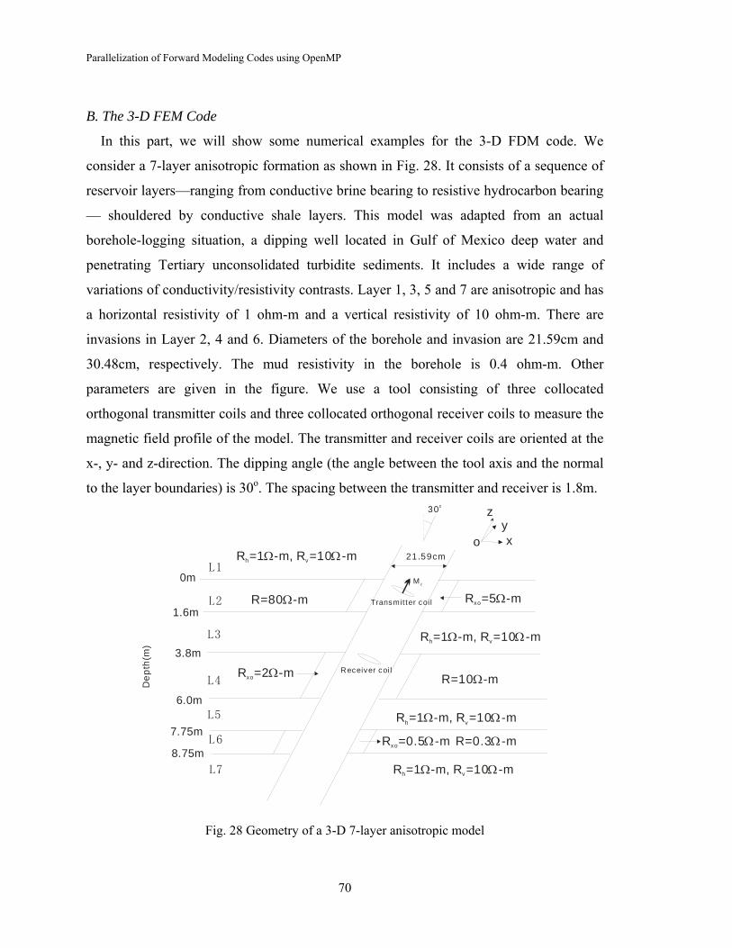
Parallelization of Forward Modeling Codes using OpenMP
70
B. The 3-D FEM Code
In this part, we will show some numerical examples for the 3-D FDM code. We
consider a 7-layer anisotropic formation as shown in Fig. 28. It consists of a sequence of
reservoir layers—ranging from conductive brine bearing to resistive hydrocarbon bearing
— shouldered by conductive shale layers. This model was adapted from an actual
borehole-logging situation, a dipping well located in Gulf of Mexico deep water and
penetrating Tertiary unconsolidated turbidite sediments. It includes a wide range of
variations of conductivity/resistivity contrasts. Layer 1, 3, 5 and 7 are anisotropic and has
a horizontal resistivity of 1 ohm-m and a vertical resistivity of 10 ohm-m. There are
invasions in Layer 2, 4 and 6. Diameters of the borehole and invasion are 21.59cm and
30.48cm, respectively. The mud resistivity in the borehole is 0.4 ohm-m. Other
parameters are given in the figure. We use a tool consisting of three collocated
orthogonal transmitter coils and three collocated orthogonal receiver coils to measure the
magnetic field profile of the model. The transmitter and receiver coils are oriented at the
x-, y- and z-direction. The dipping angle (the angle between the tool axis and the normal
to the layer boundaries) is 30o. The spacing between the transmitter and receiver is 1.8m.
L1
L2
L3
L4
L5
L6
L7
R =1 -m, R =10 -mh vΩ Ω
R =1 -m, R =10 -mh vΩ Ω
R =1 -m, R =10 -mh vΩ Ω
R=80 -mΩ
R=10 -mΩ
R=0.3 -mΩ
R =1 -m, R =10 -mh vΩ Ω
R =5 -mxo Ω
R =2 -mxo Ω
R =0.5 -mxo Ω
21.59cm
Mz
z
xy
o
Transmit ter coi l
Receiver coi l
30o
0m
1.6m
3.8m
7.75m
8.75m
Dep
th(m
)
6.0m
Fig. 28 Geometry of a 3-D 7-layer anisotropic model

Parallelization of Forward Modeling Codes using OpenMP
71
A mesh consisting 28x28x92 cells in the x-, y- and z- directions is used to model the
solution domain. For 79 observation points, Table 2 compares the CPU time cost by the
serial code and the parallel code on a 4-core computer. It can be seen that the speed of the
parallel code increase significantly as the number of core increases.
Table 2. Comparison of the CPU time cost by the serial code and parallel code
Number of cores 1 2 4 8
CPU time cost by
The serial code (mins) 192 192 192 192
CPU time cost by
The parallel code (mins) 198 132 87 56
Speedup (%) -3.1% 30.8% 54.5% 60.7%
Fig. 29 shows the calculated imaginary part of the Hxx, Hyy and Hzz responses at
100KHz using the parallel code. The results from [27] are also presented in the figure for
comparison. Good agreements are observed, validating the present parallel 3-D FDM
code. In these figures, we also present the 1-D result calculated by the 1-D analytical
method with the borehole and invasion neglected. It can be seen that the in the layers
where there are no invasions, the 1-D and 3-D results are very close to each other since
the borehole effect is not obvious in this case. However, in Layers 2, 4 and 6 where
invasions exist, the 1-D and 3-D results have discrepancy, implying that 3-D simulation
is necessary to get accurate results and more information of surrounding media.

Parallelization of Forward Modeling Codes using OpenMP
72
-1 0 1 2 3 4 5 6 7 8 9 10
-0.004
-0.002
0.000
0.002
0.004
0.006
0.008
0.010
Im(H
xx) (
A/m
)
Depth (m)
3D, present method 3D, Ref. [15] 1D, analytical method
(a) Hxx
-1 0 1 2 3 4 5 6 7 8 9 10-0.006
-0.004
-0.002
0.000
0.002
0.004
0.006
0.008
0.010
Im(H
yy) (
A/m
)
Depth (m)
3D, present method 3D, Ref. [15] 1D, analytical method
(b) Hyy
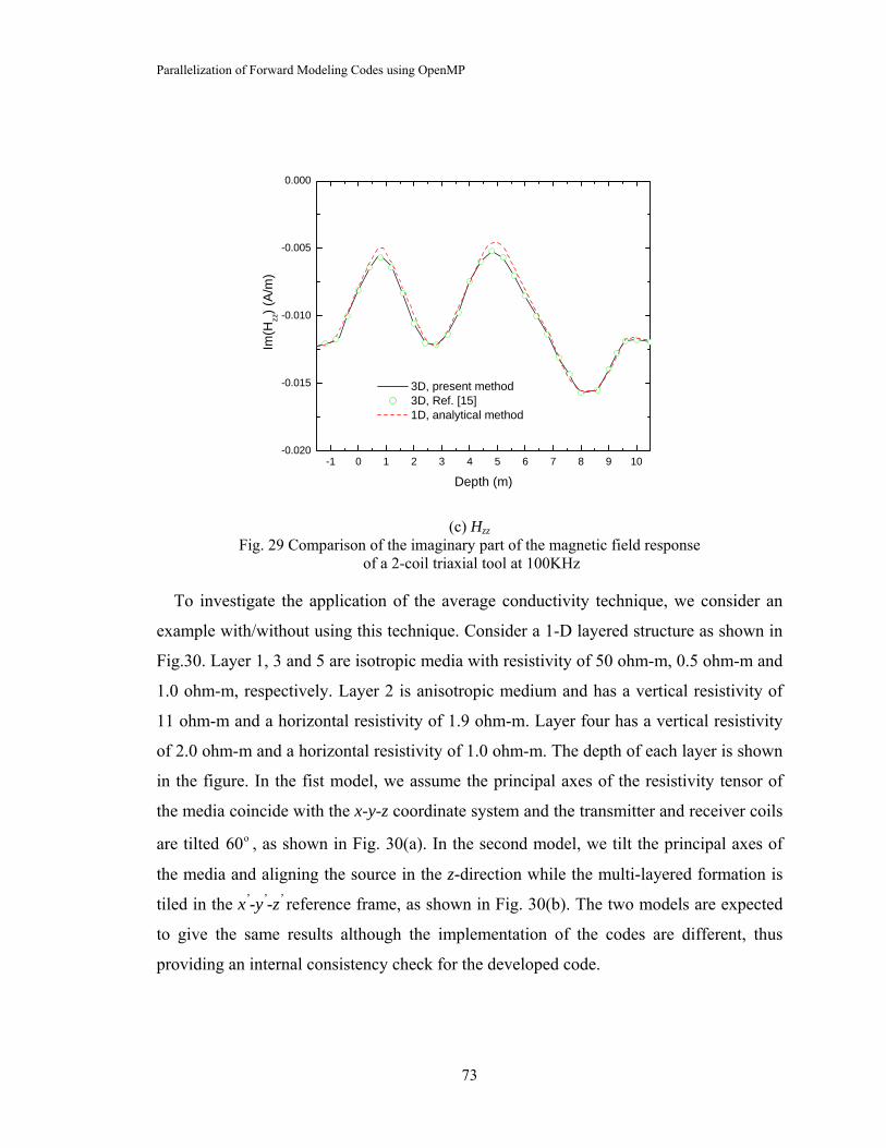
Parallelization of Forward Modeling Codes using OpenMP
73
-1 0 1 2 3 4 5 6 7 8 9 10-0.020
-0.015
-0.010
-0.005
0.000
Im(H
zz) (
A/m
)
Depth (m)
3D, present method 3D, Ref. [15] 1D, analytical method
(c) Hzz
Fig. 29 Comparison of the imaginary part of the magnetic field response of a 2-coil triaxial tool at 100KHz
To investigate the application of the average conductivity technique, we consider an
example with/without using this technique. Consider a 1-D layered structure as shown in
Fig.30. Layer 1, 3 and 5 are isotropic media with resistivity of 50 ohm-m, 0.5 ohm-m and
1.0 ohm-m, respectively. Layer 2 is anisotropic medium and has a vertical resistivity of
11 ohm-m and a horizontal resistivity of 1.9 ohm-m. Layer four has a vertical resistivity
of 2.0 ohm-m and a horizontal resistivity of 1.0 ohm-m. The depth of each layer is shown
in the figure. In the fist model, we assume the principal axes of the resistivity tensor of
the media coincide with the x-y-z coordinate system and the transmitter and receiver coils
are tilted o60 , as shown in Fig. 30(a). In the second model, we tilt the principal axes of
the media and aligning the source in the z-direction while the multi-layered formation is
tiled in the x’-y’-z’ reference frame, as shown in Fig. 30(b). The two models are expected
to give the same results although the implementation of the codes are different, thus
providing an internal consistency check for the developed code.

Parallelization of Forward Modeling Codes using OpenMP
74
In the first model, there is no need to simulate the averaged conductivity tensor since
the meshes coincide with the boundaries of the layers. But the axial component of the
magnetic field is a combination of the field generated by an x-directed source and a z-
directed source. In the second model, the meshes do not coincide with the formation
boundaries any more, so we need to calculate the averaged conductivity tensor for all the
cells. It should be noted that the conductivity tensors for each cell in the original principle
coordinate system x-y-z should be transformed to the new coordinate system x’-y’-z’
before they are used to get the averaged conductivity tensors. The transformation can be
performed by multiplying the original conductivity tensor with a rotation matrix R,
( ), ,Txx yy zzdiagσ σ σ σ′ = R R (40)
The rotation matrix R can be expressed by
⎥⎥⎥
⎦
⎤
⎢⎢⎢
⎣
⎡=
θθφθφφθφθφφθ
cos0sin-sinsincossincoscossinsin-coscos
R (41)
where θ and φ are the two Euler angles corresponding to the dip and strike angles of the
laminations. After rotation, the conductivity tensor will be a full tensor in the coordinate
system x’-y’-z’ in stead of a diagonal tensor in the original coordinate system x-y-z. Fig.
31 shows the calculated magnetic field Hxx (both the transmitter coil and receiver coils
are in the x direction) and Hzz (both the transmitter and receiver coils are in the y
direction) at different vertical depth for a pair of transmitter and receiver spaced by
1.016m and working at 20KHz. Perfect agreement is observed between the results from
the two different models, verifying the implementation of finite-difference method and
the averaged conductivity tensor calculation.
In Fig. 31, besides the results for the anisotropic case, we also present the Hxx and Hzz
for the isotropic case, namely, Layer 2 and Layer 4 are also isotropic with resistivity
being 1.0ohm-m and 1.9 ohm-m, respectively. From Fig. 31(c) and (d), we can see that
the z-directed coupling Hzz are the same in the isotropic and anisotropic cases, implying
that Hzz has no sensitivity to the vertical resistivity. On the contrary, Fig. 31 (a) and (b)
shows that the x-directed coupling Hxx can detect the anisotropy property of the media.

Parallelization of Forward Modeling Codes using OpenMP
75
TZ0.61m
-1.83m
4.88m
8.53m
Rh=Rv=0.5ohm-m
Rh=1ohm-mRv=2ohm-m
Rh=Rv=1.0ohm-m
Rh=1.9ohm-mRv=11ohm-m
Rh=Rv=50ohm-m
RZ
1.016
m
x
z
θ
Grid
x’
z’
TX
RX
(a) Model 1
RZ
Rh=Rv=0.5ohm-m
Rh=Rv=1ohm-m
Rh=Rv=50ohm-m
xz’
Grid
x’
z
1.016m
θ
TZ
TX
RX
Rh=1ohm-m, Rv=2ohm-m
Rh=1.9ohm-m, Rv=11ohm-m
(b) Model 2
Fig. 30 Two models constructed for an internal consistency check of the average conductivity technique

Parallelization of Forward Modeling Codes using OpenMP
76
-5 0 5 10 15
-0.0795
-0.0790
-0.0785
-0.0780
-0.0775
-0.0770
-0.0765
-0.0760
-0.0755
Rea
l(Hxx
) (A
/m)
Depth (Meter)
Anisotropic, Model 1 Isotropic, Model 1 Anisotropic, Model 2 Isotropic, Model 2
(a) Real (Hxx)
-5 0 5 10 15
-0.002
0.000
0.002
0.004
0.006
Imag
(Hxx
) (A
/m)
Depth (Meter)
Anisotropic, Model 1 Isotropic, Model 1 Anisotropic, Model 2 Isotropic, Model 2
(b) Imag (Hxx)

Parallelization of Forward Modeling Codes using OpenMP
77
-5 0 5 10 15
0.147
0.148
0.149
0.150
0.151
0.152
Anisotropic, Model 1 Isotropic, Model 1 Anisotropic, Model 2 Isotropic, Model 2
Rea
l(Hzz
) (A
/m)
Depth (Meter)
(c) Real (Hzx)
-5 0 5 10 15-0.002
0.000
0.002
0.004
0.006
0.008
0.010
0.012
0.014
0.016
0.018
0.020
Anisotropic, Model 1 Isotropic, Model 1 Anisotropic, Model 2 Isotropic, Model 2
Imag
(Hzz
) (A
/m)
Depth (Meter)
(d) Imag (Hzz)
Fig. 31The calculated magnetic field from the two models

Parallelization of Forward Modeling Codes using OpenMP
78
The 3-D FDM code can also be used to study the response of arbitrarily oriented
transmitter-receiver pairs which are usually used in geosteering. We consider the example
shown in Fig.16 again. In Fig.32, we also present the results of an anisotropic case for
comparison, in which the center layer has a horizontal resistivity of 4 ohm-m and a
vertical resistivity of 20 ohm-m. From the figure, we can see that the existing of the
anisotropy in the center layer changes the polarity of the phase shift and attenuation, as
shown by the dotted curves between 4-8 m.
-8 -4 0 4 8 12
-2
0
2
4
6
8
Anisotropic:Rh=4 ohm-mRv=20 ohm-m
5 ohm-m
Isotropic: 20 ohm-m
2 ohm-m
Am
plitu
de A
ttenu
atio
n (d
B)
True Vertical Depth (meter)
100KHz,Isotropic 400KHz,Isotropic 100KHZ, Anisotropic 400kHZ, Anisotropic
(a) Amplitude Attenuation

Parallelization of Forward Modeling Codes using OpenMP
79
-8 -4 0 4 8 12-40
-20
0
20
40
Anisotropic:Rh=4 ohm-mRv=20 ohm-m
5 ohm-mIsotropic: 20 ohm-m2 ohm-m
Pha
se S
hift
(deg
rees
)
True Vertical Depth (meter)
100KHz, Isotropic 400KHz, Isotropic 100KHz, Anisotropic 400KHz, Anisotropic
(b) Phase shift
Fig. 32 The response of a tilted transmitter-receiver pair in a 3-layer isotropic/anisotropic media
4. Conclusions
In this report, we use OpenMP to parallel the 1-D analytical forward modeling code
and 3-D FDM code for the simulation of wireline induction/LWD triaxial tools in
anisotropic formation. The implementation of the parallelization was described.
Numerical examples were presented to demonstrate the efficiency of the parallel code.
Then the codes were used to investigate some interesting problems. The parallelization of
the forward modeling codes significantly increases the efficiency of the original codes
and renders future real-time inversion possible.

Parallelization of Forward Modeling Codes using OpenMP
80
References
[1] W. Gropp and E. Lusk, A Test Implementation of the MPI Data Message-Passing
Standard, Technical Report ANL-92/47, December 1992.
[2] W. Gropp, E. Lusk, N. Doss and A. Skjellum, “A high-Performance, portable
implementation of the MPI Message-Passing Interface standard,” Parallel
Computing, vol. 22, pp. 789–828, 1996.
[3] G. Krawezik, F. Cappello, “Performance comparison of MPI and OpenMP on shared
memory multiprocessors,” Concurrency and Computation: Practice & Experience,
vol.18, issue. 1, pp.29-61, 2003.
[4] I. Dorta, C. Leon, C. Rodriguez, “A comparison between MPI and OpenMP branch-
and-bound skeletons,” Proceedings of the International Parallel and Distributed
Processing Symposium, 2003.
[5] R. Chandra, R. Menon, L. Dagum, D. Kohr, D. Maydan, J. McDonald, Parallel
Programming in OpenMP, Morgan Kaufmann, San Francisco, 2000.
[6] B. Chapman, G. Jost, R. van der Pas, D.J. Kuck, Using OpenMP: Portable Shared
Memory Parallel Programming, The MIT Press, Massachusetts, 2007.
[7] M. Hermanns, “Parallel Programming in Fortran 95 using OpenMP,”
http://www.openmp.org/presentations/miguel/F95-OpenMPv1-v2.pdf, 2002.
[8] C. Bischof, M. Bucker, P. Gibbon, G. Joubert, T. Lippert, Parallelizing a Real-Time
Steering Simulation for Computer Games with OpenMP, IOS Press, Netherlands,
2008.
[9] B. Kriegshäuser, O. Fanini, S. Forgang, G. Itskovich, M. Rabinovich, L. Tabarovsy, L.
Yu, M. Epov, P. Gupta, and J. V. D. Horst, “A new multicomponent induction logging
tool to resolve anisotropic formations,” Trans. SPWLA 41st Annual Logging Symp.,
Paper D Dallas, TX, 2000.
[10] M. Zhdanov, D. Kennedy, and E. Peksen, “Foundations of tensor induction well-
logging,” Petrophysics, vol. 42, no. 6, pp. 588–610, Nov./Dec. 2001.

Parallelization of Forward Modeling Codes using OpenMP
81
[11] B. Anderson, T. Barber, and T. M. Habashy, “The interpretation and inversion of
fully triaxial induction data: a sensitivity study,” 36th Annual Logging Symposium
Transactions, Society of Professional Well Log Analyst, Paper O, 2002.
[12] R. Rosthal, T. Barber, S. Bonner, K. C. Chen, S. Davydycheva, G. Hazen, D. Homan,
C. Kibbe, G. Minerbo, R. Schlein, L. Villegas, H. Wang, and F. Zhou, “Field test
result of an experimentally fully-triaxial induction tool,” Trans. SPWLA 44th Annual
Logging Symposium, Paper QQ, Galveston, TX, 2003.
[13] M. Rabinovich, L. Tabarovsky, B. Corley, J. van der Horst, and M. Epov,
“Processing multi-component induction data for formation dips and anisotropy,”
Petrophysics, vol.47, no.6, pp.506–526, 2006.
[14] M. Rabinovich, M. Gonfalini, T. Rocque, B. Corley, D. Georgi, L. Tabarovsky, and
M. Epov, “Multi-component induction logging: 10 years after,” 48th Annual Logging
Symposium, Society of Professional Well Log Analysts, 2007.
[15] Z.Y. Zhang, L.M. Yu, B. Kriegshaauser, and R. Chunduru, “Simultaneous
determination of relative angles and anisotropic resistivity using multicomponent
induction logging data,” SPWLA 42th Annual Logging Symposium, Paper Q, June 17-
20, 2001.
[16] L. L. Zhong, “”, Ph D Dissertation, University of Houston, 2004
[17] L. L. Zhong, J. Li, L.C. Shen, and R. C. Liu, “Computation of triaxial induction
logging tools in layered anisotropic dipping formations,” IEEE Trans. on Geoscience
and Remote Sensing, vol.46, no.4, pp.1148-1163, 2008.
[18] N. Yuan, X.C. Nie and R. Liu, “Responses of Triaxial Induction Tools in 1-D Multi-
Layered Transverse Isotropic Formations,” Well Logging Lab Technical Report,
Chapter 2, 2009, University of Houston
[19] M. Huang and L. C. Shen, “Computation of induction logs in multiplelayer dipping
formation,” IEEE Trans. Geosci. Remote Sens., vol. 27, no. 3, pp. 259–267, May 1989.
[20] J. H. Moran and S. Gianzero, “Effects of formation anisotropy on resistivity logging
measurement," Geophysics, vol. 44, pp.1266-1286, 1979.

Parallelization of Forward Modeling Codes using OpenMP
82
[21] K. S. Yee, “Numerical solution of initial boundary value problems involving
Maxwell’s equations in isotropic media,” IEEE Trans. Antennas Propagat., vol. 14,
no. 3, p.302-307, Jan. 1984.
[22] T. Wang and S. Fang, “3-D electromagnetic anisotropic modeling using finite
difference,” Geophysics, vol.66, no.5, p. 1386-1398, Sept-Oct 2001.
[23] Y. Saad and Schultz M. H., “GMRES: A generalized minimal residual algorithm for
solving nonsymmetric linear systems,” SIAM Journal of Sci. STAT. Comput., vol.7,
no.3, p.856-869, 1986.
[24] Y. Saad, “ILUT: A dual threshold incomplete LU factorization,” Numer. Linear
Algebra Appl., vol. 1, no. 4, p. 387–402, 1994.
[25] X. C. Nie, N. Yuan and R. Liu, “Finite-Difference Modeling of Triaxial Induction
Tools in 3D Anisotropic Media,” Well Logging Lab Technical Report, Chapter 1,
2010, University of Houston.
[26] Q. M. Li, D. Omeragic, L. Chou, L.B. Yang, K. Duong, J. Smits, J. Yang, T. Lau, C.
B. Liu, R. Dworak, V. Dreuillault, and H. Ye, “New Directional electromagnetic tool
for proactive geosteering and accurate formation evaluation while drilling,” SPWLA
46th Annual Logging Symposium, June 26-29, 2005.
[27] J. S. Hou, R. K. Mallan and C. Torres-Verdin, “Finite-difference simulation of
borehole EM measurements in 3D anisotropic media using coupled scalar-vector
potentials,” Geophysics, vol.71, no.5, p. G225-G233, Sept-Oct 2006.

Simulation of Mandrel Effect on Logging-While-Drilling Propagation Tools
83
CHAPTER 3
Simulation of Mandrel Effect on Logging-While-Drilling
Propagation Tools Abstract
We investigate the impact of the presence of collar in Logging-while-drilling (LWD)
propagation resistivity tools by simulating the tool response in various types of media
such as homogeneous isotropic formation, isotropic layered media and anisotropic
layered dipping beds. Both the transmitters and the receivers can be oriented parallel to
the tool body or perpendicular to it, thus both the z-directed and x-directed coils are
studied. The study will be focused on the effect caused by the conductive metallic drilling
collar (from now on referred to as mandrel) of LWD tool which is different from wireline
induction tools. For all the examples, two models will be studied: one treats antenna as
point-magnetic dipole without the presence of mandrel, the other models the antenna as
finite-size coils around a metallic mandrel. Simulations of both dipole model and finite
size loop coil with mandrel in one-dimensional (1-D) and two dimensional formations are
performed by the Wellog Inversion Package developed at the Well Logging Laboratory.
All the three dimensional (3-D) simulations are carried out using COMSOL RF module.
Results indicate that the presence of mandrel produces a significant (~ 0.5db) downward
shift in attenuation but has very little effect on phase-difference. By using proper
conversion charts, the Ra and Rp readings in isotropic layered dipping beds only show
differences between dipole model and model with mandrel near the bed boundary.
However, for the Ra and Rp readings in anisotropic layered dipping beds, differences
would show up even at the depths far away from the bed boundary.
1. Introduction
LWD propagation resistivity tool uses high conductive steel as mandrel due to the
high stress drilling environment. This is quite different from some wireline resistivity
tools whose mandrel is non-magnetic and non-conductive. Early studies suggest that the
Simulation of Mandrel Effect on Logging-While-Drilling Propagation Tools
84
presence of mandrel can be ignored when simulating the tool response because very little
electromagnetic field and eddy current penetrate inside the mandrel at the MHz high
operating frequency of LWD tools [1]. Hence point-magnetic dipole model is used to
simulate the tool response of the LWD resistivity tool, similar to what is done for
wireline induction tools. Study of the impact of mandrel profile on LWD tool resistivity
transform in homogeneous formation [2] indicated the attenuation is more influenced by
that presence of metallic mandrel than the phase-shift measurement. Recent work
characterized the effects of the metallic mandrel on tilted coils in homogeneous medium
[3]. Another study in isotropic layered formation pointed out that the effect of the
mandrel is large near the bed boundary but it would not affect the result of inversion [4].
It would be very interesting to perform a comprehensive study of the mandrel effect in
layered formation for conventional and directional LWD propagation resistivity tools.
In this project, point-magnetic dipole model and the model with mandrel and finite size
antennas will be analyzed to study the effects caused by the presence of a metallic
mandrel. This study will be carried out in both homogeneous isotropic medium and
layered anisotropic media, including one-dimensional (1-D), two-dimensional (2-D) and
three-dimensional (3-D) calculations. The antennas can be conventional axial coils and
also new directional coils. The primary goal of this project is to ascertain how significant
the mandrel effect is in different cases, and then decide whether and how the effect can
be corrected in interpretation.
The simulation of point-magnetic dipole models can be easily accomplished by
running existing WLL layered 1-D code for homogeneous isotropic formation and
layered anisotropic dipping beds. The model with mandrel can be simulated in radial 1-D
calculation for homogeneous or radial-layered formation. For the model with mandrel,
we use 2-D calculation to simulation tool responses in horizontal-layered formation. All
the calculations mentioned above are carried out with the WLL Wellog Inversion
software. If the model with mandrel is in layered-dipping beds, the problem becomes
three-dimensional in nature. The commercial software COMSOL RF module is used to
carry out all the 3-D calculations in this project.

Simulation of Mandrel Effect on Logging-While-Drilling Propagation Tools
85
2. Theory and Models
2.1 Principle of LWD propagation resistivity tool
The principle of LWD propagation resistivity tool has been described in many
literatures. A good introduction can be found in Ref. [1-2]. Figure 1 is a basic
configuration of a LWD resistivity tool. It consists of one transmitter and two receivers.
Since LWD resistivity tools usually operate at frequencies in the range of 100 kHz to
2MHz, typically 2 MHz, 500 kHz and 400 kHz, the skin effect at these frequencies in
rock formations is sufficiently high for us to detect the phase shift and attenuation
directly. Also because of the high frequency, the effect of dielectric constant no longer
can be ignored. We measure the signals at the two receivers, and then convert the phase
shift and amplitude ratio of these two signals to phase-shift resistivity (Rp) and
attenuation resistivity (Ra), respectively, using a chart built from homogeneous
formations and some simple dielectric relations between dielectric constant and the
formation resistivity
Figure 1 Wave Propagation Resistivity Operating Principle (from TRACS International, Ltd [5])
In the simulations, we start from Maxwell's equations to derive voltage responses on
each receiver and further obtain the phase-shift and amplitude ratio by taking the ratio of
complex voltages on the two receivers. Utilizing a pre-built converting chart, we can
convert tool response (phase-shift and amplitude ratio) in multi-layered formation into

Simulation of Mandrel Effect on Logging-While-Drilling Propagation Tools
86
apparent phase-shift and attenuation conductivity. The main steps of our approach are
shown in Figure 2. The corresponding relationship between tool response (phase-shift
and amplitude ratio) in the homogeneous medium and the conductivity of the
homogeneous medium is referred to as "Conversion Chart" or “resistivity transform”.
Figure 2 Steps of the simulation of LWD propagation resistivity tool response
For LWD propagation resistivity tools, dielectric properties of the surrounding
formation play an important role in the response, especially when the conductivity of
formation is relatively low. So we can not ignore the dielectric effect in LWD
propagation resistivity tool simulation. Moreover, in order to derive a resistivity curve
from phase-shift and attenuation separately for LWD propagation tool, the dielectric
constant of formation is assumed to depend on the formation conductivity in a specific
way. This is known as dielectric assumptions. Different assumptions are used by different
service providers. The specific relationship between conductivity and dielectric constant
can be found in Ref. [6]. Figure 3 shows the Schlumberger arcVision resistivity tool
configuration. For Schlumberger 2 MHz propagation resistivity measurement, dielectric
constant is assumed to be related to the conductivity by the following formula: 0.35108.5 5rε σ= ∗ + .

Simulation of Mandrel Effect on Logging-While-Drilling Propagation Tools
87
Figure 3 ARC475 from Schlumberger [6]
2.2 1-D Point-Magnetic-Dipole Model
The geometrical configuration of 1D horizontal-layered formation is depicted in Figure
4. In this model, we do not consider the presence of mandrel, and the transmitter is
treated as an infinitesimally small magnetic dipole, i.e., point magnetic dipole. In this
model, two orthogonal coils are set to be transmitters, one with magnetic moment pointed
in vertical z-direction and the other in horizontal x-direction. To simulate tool response in
this model, we need to calculate the magnetic fields produced by a z-directed magnetic
dipole and an x-directed magnetic dipole.
Figure 4 Profile of the 1-D point-magnetic dipole model
Simulation of Mandrel Effect on Logging-While-Drilling Propagation Tools
88
Note the receivers are also treated as point-magnetic-dipole and can be either z- or x-
directed.
Assuming the harmonic time dependence to be j te ω− , Maxwell’s equations for the
electric and magnetic fields are
jω∇× = − +H D J , (1a)
jω∇× =E B . (1b)
Assume no anisotropy in magnetic properties, then we can get
sμ μ= +B H M , (2a)
ˆ sσ= + JJ E , (2b)
and
ε=D E , (2c)
where sM represents the dipole-source distribution and sJ is the source distribution of
current.
Placing equations (2) into equations (1), we can get
ˆˆ( ) sjσ ωε∇× = − +H E J , (3a)
sj jωμ ωμ∇× =E H + M . (3b)
Define a complex conductivity tensor σ ′ as follows
0 0 0 0ˆ 0 0 0 0
0 0 0 0
h h h
h h h
v v v
jj
j
σ σ ωεσ σ σ ωε
σ σ ωε
′ −⎡ ⎤ ⎡ ⎤⎢ ⎥ ⎢ ⎥′ ′= = −⎢ ⎥ ⎢ ⎥
′⎢ ⎥ ⎢ ⎥−⎣ ⎦ ⎣ ⎦
, (4)
then equation (3a) will become
ˆ sσ ′∇× = +H E J . (5)

Simulation of Mandrel Effect on Logging-While-Drilling Propagation Tools
89
For LWD propagation tools, we set 0s =J . From equation (5), we can get
ˆ 0σ ′∇ • =E . (6)
This allows to introduce the hertz vector Π and a scalar potential Φ [6], such that
ˆ hjσ ωμσ= ∇×E Π , (7)
hjωμσ= +∇ΦH Π . (8)
Adopting a gauge condition
ˆ( ) vσ σ′ ′∇• •Π = Φ , (9)
we will have 1ˆhjωμσ σ −= •∇×E Π , (10)
ˆ( )( )hv
j σωμσσ′∇ • •
= +∇′ΠH Π . (11)
Substituting equation (10), (11) into equation (3b), we obtain
2 22
1x v x xk Mλ λ
∇ Π + Π = − (12)
2 22
1y v y yk Mλ λ
∇ Π + Π = − (13)
( )2 2 21 yxz h z zk M
z x yλ λ∂Π⎛ ⎞∂Π∂
∇ Π + Π = − + − +⎜ ⎟∂ ∂ ∂⎝ ⎠ (14)
where ⎟⎟⎠
⎞⎜⎜⎝
⎛∂∂
+∂∂
+∂∂
=∇ 2
2
22
2
2
22 1
zyx λλ , 2h hk iωμσ ′= , 2
v vk iωμσ ′= and /h vλ σ σ′ ′= .
2.2.1. Magnetic Field Response of Dipoles in Homogeneous Medium
For a z-directed magnetic dipole with moment (0,0, )Ts zM=M , the hertz vector is
given by [5]
ˆ4
hjk rz
zM ez
rπΠ = Π = , (15)
where 2 2 2r x y z= + + .
Simulation of Mandrel Effect on Logging-While-Drilling Propagation Tools
90
For an x-directed magnetic dipole ( ,0,0)Ts xM=M , the hertz vector is given by
ˆ ˆx zx z= Π +ΠΠ , (16)
where
4
vjk sx
xM e
sπλΠ = , (17)
24
v hjk s jk rx
zM x e ez
s rλ
πρ⎛ ⎞
Π = −⎜ ⎟⎝ ⎠
, (18)
2 2 2 2s x y zλ= + + , (19)
and
2 2x yρ = + . (20)
Placing equation (15)-(20) into (11), we can get the magnetic field response of the
magnetic dipole with moment in x-directed and z-directed ( , , ) ( )s x y zM M M δ=M r in a
homogeneous transverse isotropic medium as follows
2 2 2
2 4
24
vjk sh h h v h
xxk jk s k k x jk xeH
s sπ λ ρ ρ⎡ ⎤−
= + −⎢ ⎥⎣ ⎦
( )2 22 2 2 2 2
2 4 2 3 4 5
12 3 34
hjk rhh h h h h
k xjk r k x jk x jk jk xe xr r r r rπ ρ ρ
⎡ ⎤+−⎢ ⎥− − − + + −⎢ ⎥⎣ ⎦
, (21)
23 2
3 34
hjk rh
xz zx hjkeH H xz k
r r rπ⎡ ⎤= = − + −⎢ ⎥⎣ ⎦
, (22)
and
( )2 2 2 22
2 3 4
1 3 34
hjk rhh h
zz h
k zjk jk ze zH kr r r r rπ
⎡ ⎤+⎢ ⎥= + − − +⎢ ⎥⎣ ⎦
. (23)
Here ijH represents i-directed component of the magnetic field due to j-directed dipole
moment of the source sM .

Simulation of Mandrel Effect on Logging-While-Drilling Propagation Tools
91
To generate conversion charts, we need first to calculate tool response in isotropic
medium. Then equation (21)-(23) can be simplified to
2 2 2 2 2
2 3 4 5
1 3 34
jkr
xxe k jk k x jkx xH
r r r r rπ⎡ ⎤+
= + − − +⎢ ⎥⎣ ⎦
, (24)
23 2
3 3 ,4
jkr
zx xzxze jkH H k
r r rπ− ⎡ ⎤= = + −⎢ ⎥⎣ ⎦
(25)
and 2 2 2 2
22 3 4
1 3 34
jkr
zzk ze jk jkz zH k
r r r r rπ⎡ ⎤+
= + − − +⎢ ⎥⎣ ⎦
. (26)
These equations can be used to calculate the coupling between point-dipole transmitters
and receivers in homogeneous isotropic media which is then used as conversion chart.
2.2.2. Magnetic Field Response of Dipoles in Multi-layered Media
1) z-directed magnetic dipole
For the z-directed magnetic dipole, Hertz vector is given by,
ˆz z∏ =∏ . (27)
In the i-th layer ( 1i iz z z− < < ) of the formation, the hertz vector is [6-7]
000( )
4hi hi hiz z z ziz
zi i ihi
M e Fe G e J dξ ξ ξβ α αρ απ ξ
∞ − − −⎛ ⎞Π = + +⎜ ⎟
⎝ ⎠∫ , (28)
where iz is the lower boundary of the i-th layer,
( )nJ x is the n-th order Bessel function,
( )1/ 22 2hi hikξ α= −
(29)
( )1/2hi hik iωμσ ′= (30)
and
0, if is not in the -th layer1, if is in the i-th layer
zi
z
M iM
β⎧
= ⎨⎩
. (31)

Simulation of Mandrel Effect on Logging-While-Drilling Propagation Tools
92
Substituting equation (28) into (11), we can get the magnetic field as follows
0 300( )
4hi hi hiz z z ziz
zzi i ihi
MH e Fe G e J dξ ξ ξβ α αρ απ ξ
∞ − − −⎛ ⎞= + +⎜ ⎟
⎝ ⎠∫ , (32)
00 210
0
cos ( )4
hi hi hiz z z zizxzi hi i i
hi
z zMH e Fe G e J dz z
ξ ξ ξβξ α ϕ αρ απ ξ
∞ − − −⎛ − ⎞= + −⎜ ⎟−⎝ ⎠
∫ , (33)
00 210
0
sin ( )4
hi hi hiz z z zizyzi hi i i
hi
z zMH e Fe G e J dz z
ξ ξ ξβξ α ϕ αρ απ ξ
∞ − − −⎛ − ⎞= + −⎜ ⎟−⎝ ⎠
∫ . (34)
To obtain reflection and transmission coefficients iF and iG , we need to enforce
boundary conditions. From the continuity of electromagnetic fields at horizontal
boundary iz z= , the boundary conditions of hertz vector are
( 1)z izi
z z+∂Π∂Π
=∂ ∂
, (35)
1 ( 1)i zi i z iμ μ + +Π = Π . (36)
The numerical scheme developed to solve iF and iG can be found in Ref. [8].
2) x-directed magnetic dipole
For the x-directed magnetic dipole, hertz vector is given by
ˆ ˆx zx z∏ =∏ +∏ . (37)
In the i-th layer ( 1i iz z z− < < ) of the formation, the hertz vector is
000( )
4vi vi i vi iz z z zx i
xi i ii vi
M e Pe Q e J dξ ξ λ ξ λβ α αρ απλ ξ
∞ − − −⎛ ⎞Π = + +⎜ ⎟
⎝ ⎠∫ , (38)
and
( ) 10cos ( )
4hi i hi i vi i vi iz z z zx
zi i i vi i vi iM S e T e Pe Q e J dξ λ ξ λ ξ λ ξ λξ ξ φ αρ απ
∞ − −Π = + − + +∫
( )0 0 010
0
cos ( )4
hi vi iz z z zxi
z zM e e J dz z
ξ ξ λβ φ αρ απ
∞ − − − − −−
−∫ . (39)
Substituting equations (38)-(39) into (11), we can get the magnetic field as follows

Simulation of Mandrel Effect on Logging-While-Drilling Propagation Tools
93
0 02
2 2
2 2 2 200
2 2
sin cos
sin sin ( )4
cos cos
vi i hi
vi i vi i
hi hi
z z z zihi i hi
i vi
z zx i ixxi hi hi
i iz z
i hi i hi
k e e
M P QH k e k e J d
S e T e
ξ λ ξ
ξ λ ξ λ
ξ ξ
β φ β φξλξ
φ φ α αρ απ λ λ
φξ φξ
− − − −
∞ −
−
⎛ ⎞−⎜ ⎟
⎜ ⎟⎜ ⎟
= + +⎜ ⎟⎜ ⎟⎜ ⎟− +⎜ ⎟⎜ ⎟⎝ ⎠
∫
0 02
2 210
cos 2 ( )4
vi i hi
vi i vi i
hi hi
z z z zii vi i hi
vi
z zxi i vi i i vi
z zi hi i hi
k e e
M P k e Q k e J d
S e T e
ξ λ ξ
ξ λ ξ λ
ξ ξ
βλ β ξξ
φ λ λ αρ απρ
ξ ξ
− − − −
∞ −
−
⎛ ⎞+⎜ ⎟⎜ ⎟⎜ ⎟+ + +⎜ ⎟+ −⎜ ⎟⎜ ⎟⎝ ⎠
∫ , (40)
0 02
2 200
sin cos ( )4
vi i hi
vi i vi i
hi hi
z z z zihi i hi
i vi
z zx i iyxi hi hi
i iz z
i hi i hi
k e e
M P QH k e k e J d
S e T e
ξ λ ξ
ξ λ ξ λ
ξ ξ
β β ξλξ
ϕ ϕ α αρ απ λ λ
ξ ξ
− − − −
∞ −
−
⎛ ⎞− −⎜ ⎟⎜ ⎟⎜ ⎟
= − −⎜ ⎟⎜ ⎟⎜ ⎟− +⎜ ⎟⎝ ⎠
∫
0 02
2 210
sin 2 ( )4
vi i hi
vi i vi i
hi hi
z z z zii vi i hi
vi
z zxi i vi i i vi
z zi hi i hi
k e e
M P k e Q k e J d
S e T e
ξ λ ξ
ξ λ ξ λ
ξ ξ
βλ β ξξ
φ λ λ αρ απρ
ξ ξ
− − − −
∞ −
−
⎛ ⎞+⎜ ⎟⎜ ⎟⎜ ⎟+ + +⎜ ⎟+ −⎜ ⎟⎜ ⎟⎝ ⎠
∫ , (41)
00 210
0
cos ( )4
hi hi hiz z z zxzxi i i i
z zMH e S e T e J dz z
ξ ξ ξφ β α αρ απ
∞ − − −⎛ − ⎞= + +⎜ ⎟−⎝ ⎠
∫ , (42)
where
vi
hii k
k=λ , (43)
( )1/ 22 2vi vikξ α= − , (44)
( )1/2vi vik iωμσ′= , (45)

Simulation of Mandrel Effect on Logging-While-Drilling Propagation Tools
94
0, if is not in the -th layer1, if is in the -th layer
xi
x
M iM i
β⎧
= ⎨⎩
. (46)
The coefficients iP , iQ , iS and iT can be calculated by matching the boundary
conditions. From the continuity of electromagnetic fields at horizontal boundary iz z= ,
the boundary conditions of hertz vector are
( 1)1
x ixii iz z
μ μ ++
∂Π∂Π=
∂ ∂ (47)
1 ( 1)i zi i z iμ μ + +Π = Π (48)
2 22 2( 1) ( 1)2 2
12 2x i z ixi zi
i ix x z x x zλ λ + +
+
∂ Π ∂ Π∂ Π ∂ Π+ = +
∂ ∂ ∂ ∂ ∂ ∂ (49)
2 2( 1) ( 1)hi xi h i x ik k + +Π = Π (50)
The numerical scheme developed to solve iP , iQ , iS and iT can be found in Ref. [15].
We derived all the tool response in previous two parts with tool axes lining up with the
coordinates of formation beddings. However, in reality the tool axis can be arbitrary
direction with respect to the coordinate of formation. A rotation matrix is implemented to
do the transformation [16]. Explicitly, we first convert dipole moments given in tool
coordinates into formation coordinates by using rotation matrix R. That is
'R=M M , (51)
Then we do an inverse transformation when we get the magnetic field H in the
formation coordinates. So the final response in tool coordinates will be
1R−′ =H H . (52)
2.3 1-D Model of Finite-size Attennas with Mandrel
The geometrical configuration of the model with finite size antenna outside a mandrel
is shown in Figure 5. The radii of the transmitter and receivers are b. The outer boundary

Simulation of Mandrel Effect on Logging-While-Drilling Propagation Tools
95
of the m-th region is denoted mr ; and mε , mσ and mμ represent respectively the dielectric
constant, the conductivity and the magnetic permeability.
Figure 5 Profile of 1-D radial-layered media
Assuming azimuthally symmetry, the electric field φE in region 2 can be expressed as
following [11]:
∫∞
+−=0
212
2 ])[cos(2
WWkzdkIb
EE sωμ
φ (53)
where
)(][12
)2(1
)22(122
)22(2211
12212 bhepqepqD
W rrjrbj λλλ −−−− −= (54)
)(][12
)1(1
)22(211
)22(1122
12222 bhepqepqD
W rrjrbj λλλ −−+−− −= (55)
)22(21121122
122 rrjeppppD −−−= λ (56)
Simulation of Mandrel Effect on Logging-While-Drilling Propagation Tools
96
)()( 12)2(
111
112
)2(0
2
211 rhgrhp λ
μλ
λμλ
−= (57)
)()( 12)1(
111
112
)1(0
2
212 rhgrhp λ
μλ
λμλ
−= (58)
)()( 22)2(
133
322
)2(0
2
221 rhGrhp λ
μλ
λμλ
−= (59)
)()( 22)1(
133
322
)1(0
2
222 rhGrhp λ
μλ
λμλ
−= (60)
)()]()([ 22
112111
1120
2
21 bhrjgrjq λλ
μλ
λμλ
−−= (61)
)( 21212 bjpq λ−= (62)
)()(
111
1101 rj
rjg
λλ
= , (63)
and sE is the electric field due to the source in a homogeneous medium characterized by
the medium 2 parameters. It can be expressed as follow:
∫−
−−=
π
π
φφπ
ωμR
edIbj
ERjk
s
2
cos4
2 , (64)
where
21
222 )cos22( φbbzR −+= (65)
)()(
23)2(
1
23)2(
03 rh
rhG
λλ
= . (66)
The voltage induced at the receiving coil is equal to 22 φπbE .
When we build converting chart in this 1D cylindrical layered medium, we set the
conductivity to be infinity in region 1 (collar) which is characterized by perfect conductor
parameters. For normal steel collar/mandrel, this is an excellent approximation at MHz
frequency. The conductivities of other regions are all set to be the same as formation.

Simulation of Mandrel Effect on Logging-While-Drilling Propagation Tools
97
2.4 2-D and 3-D Model
Z-directed coils in horizontal layers. Figure 6 shows a model which can have layers
both in vertical direction and in radial direction. The tool is positioned at the center of the
borehole and the transmitter and receiver coils are all z-directed. Due to axis-symmetry,
this is a 2-D model. In this thesis, this 2-D model will be studied both with MWD2D99
code inside Wellog Inversion Package and with RF Module of a commercial multiphysics
modeling package called COMSOL (from now on referred to as COMSOL).
Figure 6 Schematic of 2-D model
Figure 7 shows the 2-D axis-symmetric model setup in COMSOL. A large rectangular
domain is selected so the boundary is far away from the tool which is put in the center of
the domain. The metallic mandrel is shown as a narrow black box in the middle and the
locations of the transmitter and receivers are indicated as well. Finite size transmitter and
receiver loop antenna are represented by a point in the r-z plan due to axis-symmetry. A
line source ( 1I A= ) was assigned to “T” point serving as transmitter. Complex voltages
were calculated on the two receivers to obtain amplitude ratio and phase difference. At
r=0 axis, axis-symmetry condition was added. Radial depth of the surrounding formation
was set to be slightly more than 5 times the skin-depth which ensures the signal decays
sufficiently small at the boundary. Scattering boundary condition was set to the outer

Simulation of Mandrel Effect on Logging-While-Drilling Propagation Tools
98
boundary. Alternatively the impedance boundary condition can be applied at the edge of
the overall domain to reduce the size to simulation domain [12].
Figure 7 Geometry of 2-D axis-symmetric model in COMSOL.
Finite size z-directed coils with mandrel in dipping beds. For cases like finite size
antennas with mandrel in dipping layered beds, they are not axis-symmetrical any more.
They are genuinely 3-D models as shown in Figure 8. In this report, calculations on these
3-D models will be conducted in COMSOL. Figure 9 shows an example of model
geometry of the z-directed coil with mandrel in homogeneous medium. Again the outer
box represents the surrounding formation. The cylinder represents metallic mandrel.
Three circles represent transmitter and receiver coils. An edge current is used to excite
the transmitter. For ease of simulation, the transmitter and receiver are modeled as finite
size loop with an infinitesimal thin wire. In actual tools, multiple windings are typically
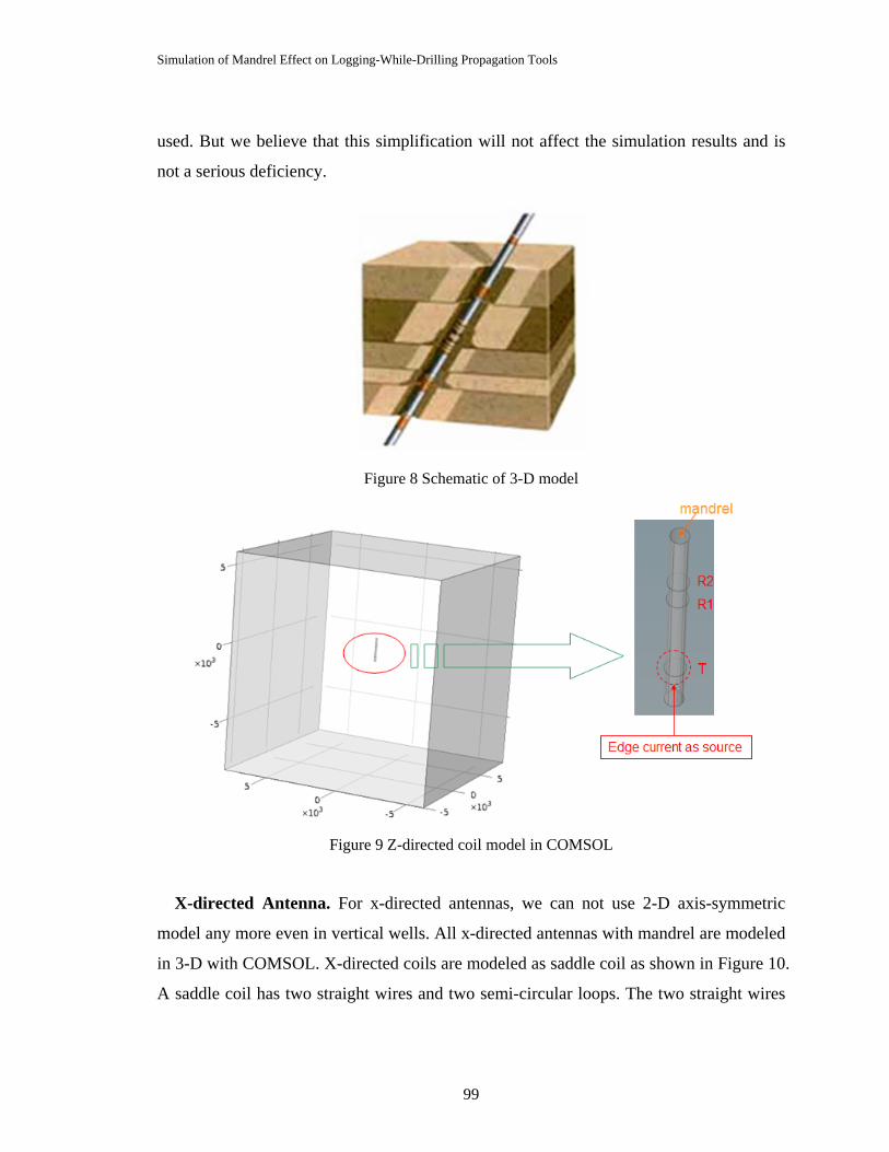
Simulation of Mandrel Effect on Logging-While-Drilling Propagation Tools
99
used. But we believe that this simplification will not affect the simulation results and is
not a serious deficiency.
Figure 8 Schematic of 3-D model
Figure 9 Z-directed coil model in COMSOL
X-directed Antenna. For x-directed antennas, we can not use 2-D axis-symmetric
model any more even in vertical wells. All x-directed antennas with mandrel are modeled
in 3-D with COMSOL. X-directed coils are modeled as saddle coil as shown in Figure 10.
A saddle coil has two straight wires and two semi-circular loops. The two straight wires

Simulation of Mandrel Effect on Logging-While-Drilling Propagation Tools
100
are parallel to the tool axis. The semi-circular loops with a radius of 3.5” are concentric to
the collar.
Figure 10 Saddle coil as x-directed dipole
Typically a pair of saddle coils is connected to form the actual saddle coil which will
generate a more symmetric filed and in turn reduce the potential excitation of unwanted
mode in borehole.
In constructing the models, we need to be aware that the size of the geometry could be
very large in less conductive formation. Therefore, finer meshes should be adopted to
ensure the convergences in less conductive formation.
3. Results and Analysis
The main goal of the project is to compare responses between point-dipole model and
finite-loop-with-mandrel model to determine when a point-dipole model no longer is
sufficient to interpret LWD propagation resistivity tool. This section will show all the 1-
D, 2-D and 3-D calculations for z-directed and x-directed coils of both point-dipole
model and model with mandrel in various types of media such as laminated isotropic
beddings and anisotropic dipping beds.
3.1 Results of Z-directed coils
1) In homogeneous isotropic medium
Figure 11 shows one example of electric field distribution from a z-directed loop
dipole of LWD propagation resistivity tool operating at 2MHz in homogeneous isotropic
Mandrel Saddle Coil

Simulation of Mandrel Effect on Logging-While-Drilling Propagation Tools
101
medium (0.1 S/m conductivity), produced by an axis-symmetrical 2-D model using
COMSOL. The mesh is chosen sufficiently fine so the field is smooth. This is evident
from the figure and the observation that even though the simulation space is rectangular,
the dipole field is well represented even close to the boundary. This is also an ideal case
where the skin depth is such that the field has been attenuated many orders of magnitude
at the boundary.
We have simulated LWD tool with TR spacing 28-in. and RR spacing of 6-in. in
homogeneous isotropic formation with the conductivity varying from 0.005 to 5 S/m. The
characteristic plots (referred to as Conversion Chart) of attenuation and phase-shift versus
formation resistivity are shown in Figure 12 and Figure 13, respectively. The absolute
differences between different charts are shown in Figure 14. Note the Schlumberger
dielectric assumption is used in all simulations. From the charts, we can see that the
results from the analytical code and those from COMSOL 2-D and 3-D models agree
very well. It is gratify to see such excellent agreement between COMSOL results and
results form analytical code. We also notice that the presence of mandrel produces a
significant (~ 0.5db) downward shift in attenuation but has very little effect on phase-
difference. This is consistent with the conclusion from an earlier study [2]. This
difference in attenuation would not necessarily make the dipole-model unusable for
interpretation. It only means we cannot use the same conversion chart between different
models. In other words, each model has to use its own conversion chart. The more
important question is whether the apparent resistivity would behave differently once the
appropriate conversion chart is used. In the following sections, we will use the
conversion charts shown in Figure 12-13 to convert amplitude ratio and phase difference
in layered media to attenuation resistivity (Ra) and phase-shift resistivity (Rp),
respectively.

Simulation of Mandrel Effect on Logging-While-Drilling Propagation Tools
102
Figure 11 E field distributions in homogeneous medium. The r and z units are in millimeters.
5 6 7 8 9 10 11 12 1310-1
100
101
102
103
Attenuation (dB )
Ra
(Ohm
-m)
Converting Chart for Ra
W ithout mandrel (From code)With mandrel (From code)With mandrel (From COMSOL 2D )With mandrel (From COMSOL 3D )
Figure 12 Conversion chart for Ra
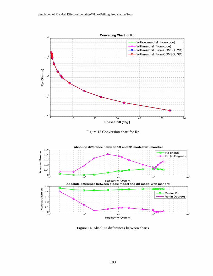
Simulation of Mandrel Effect on Logging-While-Drilling Propagation Tools
103
0 10 20 30 40 50 6010
-1
100
101
102
103
Phase Shift (deg.)
Rp
(Ohm
-m)
Converting Chart for Rp
Without mandrel (From code)With mandrel (From code)With mandrel (From COMSOL 2D)With mandrel (From COMSOL 3D)
Figure 13 Conversion chart for Rp
10-1 100 101 102 1030
0.01
0.02
0.03
0.04
0.05
Resistivity (Ohm-m)
Abs
olut
e di
ffere
nce
Absolute difference between 1D and 3D model with mandrel
Ra (in dB)Rp (in Degree)
10-1 100 101 102 1030
0.1
0.2
0.3
0.4
0.5
Resistivity (Ohm-m)
Abs
olut
e di
ffere
nce
Absolute difference between dipole model and 3D model with mandrel
Ra (in dB)Rp (in Degree)
Figure 14 Absolute differences between charts

Simulation of Mandrel Effect on Logging-While-Drilling Propagation Tools
104
2) In isotropic layered dipping beds
Dipole model response in isotropic layered dipping beds can be obtained from 1D
simulation code from the WLL Inversion Package. The study of the response of the tool
with finite size antenna with mandrel requires 3D codes and COMSOL modeling package
is used. Figure 15 indicates the profile of the formation. The tool responses are shown in
Figure 16 and Figure 17 for dip = 60 deg. The depths shown in figures are measured
depth (MD). The bed boundary is at zero MD. We can see that mandrel effect only
affects Ra and Rp readings near the bed boundary.
Figure 15 Profile of a 2-layer isotropic media
60 degree
σ=0.5 S/m
σ=5 S/m
25 ft.
15 ft.

Simulation of Mandrel Effect on Logging-While-Drilling Propagation Tools
105
-15 -10 -5 0 510
-1
100
Ra
(Ohm
-m)
Depth (ft.)
With mandrel (From COMSOL)Without mandrel (From code)Rt
Figure 16 Ra from dipole model and mandrel model
-15 -10 -5 0 510-1
100
Rp
(Ohm
-m)
Depth (ft.)
With mandrel (From COMSOL)Without mandrel (From code)Rt
Figure 17 Rp from dipole model and mandrel model
3) In anisotropic layered dipping beds

Simulation of Mandrel Effect on Logging-While-Drilling Propagation Tools
106
In dipping beds, the effect of anisotropy can be detected by z-directed coils. Early
study [13] showed that LWD resistivity measurements from z-directed coils have higher
sensitivity to anisotropy at higher dipping angles. This project studied anisotropic cases
with dipping angle at 60 degrees and 80 degrees.
Figure 18 is the profile of the first example of the anisotropy cases. The dipping angle
is 60 degree. For both layers, the conductivity of horizontal direction is 1 S/m. The
anisotropy ratio Rv / Rh for the upper layer and lower layer is chosen to be 10 and 2,
respectively, so that we can analyze the mandrel effect in Ra and Rp readings contributed
by anisotropy. The Ra and Rp logs are shown in Figure 19 and 20, respectively.
Figure 18 Profile of a 2-layer anisotropic formation
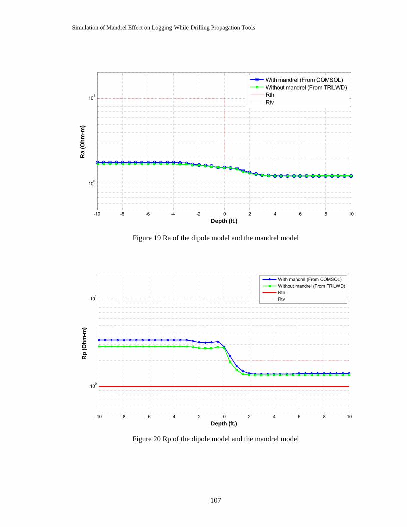
Simulation of Mandrel Effect on Logging-While-Drilling Propagation Tools
107
-10 -8 -6 -4 -2 0 2 4 6 8 10
100
101
Ra
(Ohm
-m)
Depth (ft.)
With mandrel (From COMSOL)Without mandrel (From TRILWD)RthRtv
Figure 19 Ra of the dipole model and the mandrel model
-10 -8 -6 -4 -2 0 2 4 6 8 10
100
101
Rp
(Ohm
-m)
Depth (ft.)
With mandrel (From COMSOL)Without mandrel (From TRILWD)RthRtv
Figure 20 Rp of the dipole model and the mandrel model
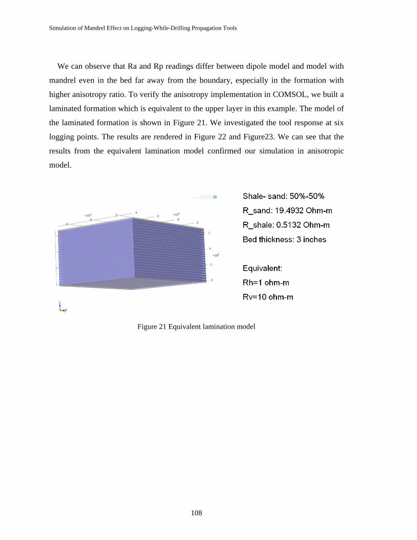
Simulation of Mandrel Effect on Logging-While-Drilling Propagation Tools
108
We can observe that Ra and Rp readings differ between dipole model and model with
mandrel even in the bed far away from the boundary, especially in the formation with
higher anisotropy ratio. To verify the anisotropy implementation in COMSOL, we built a
laminated formation which is equivalent to the upper layer in this example. The model of
the laminated formation is shown in Figure 21. We investigated the tool response at six
logging points. The results are rendered in Figure 22 and Figure23. We can see that the
results from the equivalent lamination model confirmed our simulation in anisotropic
model.
Figure 21 Equivalent lamination model
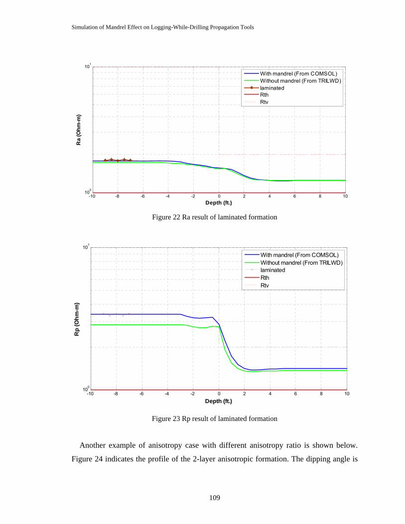
Simulation of Mandrel Effect on Logging-While-Drilling Propagation Tools
109
-10 -8 -6 -4 -2 0 2 4 6 8 10100
101
Ra
(Ohm
-m)
Depth (ft.)
With mandrel (From COMSOL)Without mandrel (From TRILWD)laminatedRthRtv
Figure 22 Ra result of laminated formation
-10 -8 -6 -4 -2 0 2 4 6 8 10100
101
Rp
(Ohm
-m)
Depth (ft.)
With mandrel (From COMSOL)Without mandrel (From TRILWD)laminatedRthRtv
Figure 23 Rp result of laminated formation
Another example of anisotropy case with different anisotropy ratio is shown below.
Figure 24 indicates the profile of the 2-layer anisotropic formation. The dipping angle is
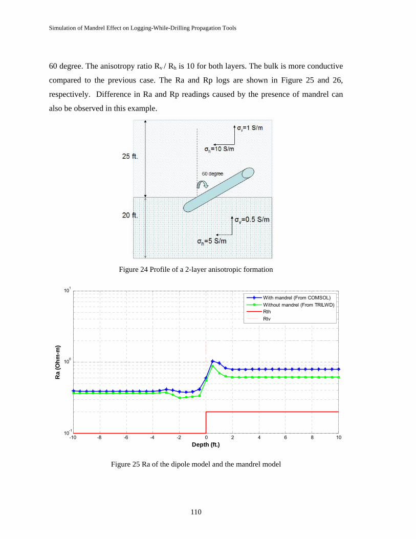
Simulation of Mandrel Effect on Logging-While-Drilling Propagation Tools
110
60 degree. The anisotropy ratio Rv / Rh is 10 for both layers. The bulk is more conductive
compared to the previous case. The Ra and Rp logs are shown in Figure 25 and 26,
respectively. Difference in Ra and Rp readings caused by the presence of mandrel can
also be observed in this example.
Figure 24 Profile of a 2-layer anisotropic formation
-10 -8 -6 -4 -2 0 2 4 6 8 1010-1
100
101
Ra
(Ohm
-m)
Depth (ft.)
With mandrel (From COMSOL)Without mandrel (From TRILWD)RthRtv
Figure 25 Ra of the dipole model and the mandrel model
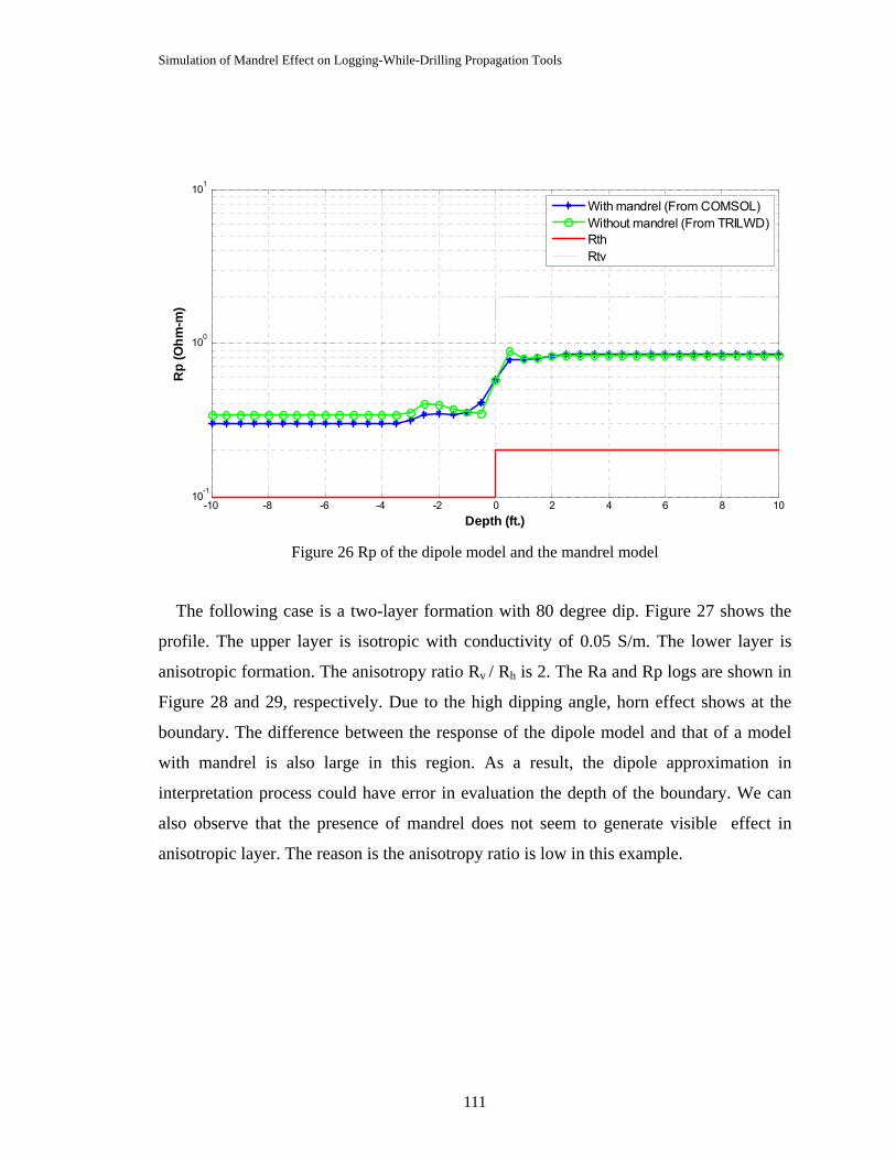
Simulation of Mandrel Effect on Logging-While-Drilling Propagation Tools
111
-10 -8 -6 -4 -2 0 2 4 6 8 1010-1
100
101R
p (O
hm-m
)
Depth (ft.)
With mandrel (From COMSOL)Without mandrel (From TRILWD)RthRtv
Figure 26 Rp of the dipole model and the mandrel model
The following case is a two-layer formation with 80 degree dip. Figure 27 shows the
profile. The upper layer is isotropic with conductivity of 0.05 S/m. The lower layer is
anisotropic formation. The anisotropy ratio Rv / Rh is 2. The Ra and Rp logs are shown in
Figure 28 and 29, respectively. Due to the high dipping angle, horn effect shows at the
boundary. The difference between the response of the dipole model and that of a model
with mandrel is also large in this region. As a result, the dipole approximation in
interpretation process could have error in evaluation the depth of the boundary. We can
also observe that the presence of mandrel does not seem to generate visible effect in
anisotropic layer. The reason is the anisotropy ratio is low in this example.

Simulation of Mandrel Effect on Logging-While-Drilling Propagation Tools
112
Figure 27 Profile of a 2-layer anisotropic formation
-20 -15 -10 -5 0 5 10 15 20100
101
102
103
Ra
(Ohm
-m)
Depth (ft.)
With mandrel (From COMSOL)Without mandrel (From TRILWD)RthRtv
Figure 28 Ra of the dipole model and the mandrel model
80 degree
σv=0.5 S/m
25 ft.
20 ft.
σh=1 S/m
σ =0.05 S/m

Simulation of Mandrel Effect on Logging-While-Drilling Propagation Tools
113
-20 -15 -10 -5 0 5 10 15 20100
101
102
103
104
Rp
(Ohm
-m)
Depth (ft.)
With mandrel (From COMSOL)Without mandrel (From TRILWD)RthRtv
Figure 29 Rp of the dipole model and the mandrel model
From previous examples, we know that the effect caused by the presence of mandrel is
larger when the anisotropy ratio is higher. Table 2 shows 7 cases of tool response in
anisotropic homogeneous formation with anisotropy ratio at 10 and 20. We can see that
the difference from Ra and Rp can be up to 0.6 Ohm-m and 1.8 Ohm-m, respectively.
Table 2 Tool response in anisotropic homogeneous formation
3.2 Results of x-directed coils
1) In homogeneous isotropic medium
Figure 30-31 are two examples of E field distributions of x-directed coil in
homogeneous medium in xy-plane and yz-plane, respectively. Phase-difference and
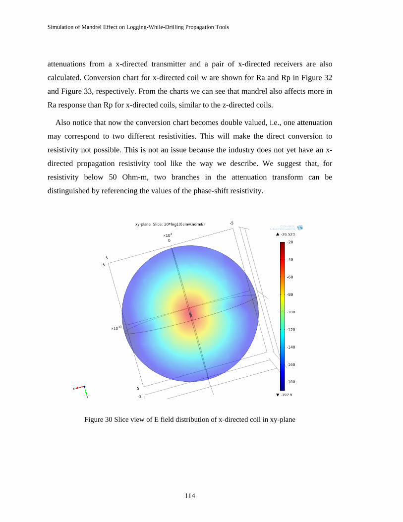
Simulation of Mandrel Effect on Logging-While-Drilling Propagation Tools
114
attenuations from a x-directed transmitter and a pair of x-directed receivers are also
calculated. Conversion chart for x-directed coil w are shown for Ra and Rp in Figure 32
and Figure 33, respectively. From the charts we can see that mandrel also affects more in
Ra response than Rp for x-directed coils, similar to the z-directed coils.
Also notice that now the conversion chart becomes double valued, i.e., one attenuation
may correspond to two different resistivities. This will make the direct conversion to
resistivity not possible. This is not an issue because the industry does not yet have an x-
directed propagation resistivity tool like the way we describe. We suggest that, for
resistivity below 50 Ohm-m, two branches in the attenuation transform can be
distinguished by referencing the values of the phase-shift resistivity.
Figure 30 Slice view of E field distribution of x-directed coil in xy-plane
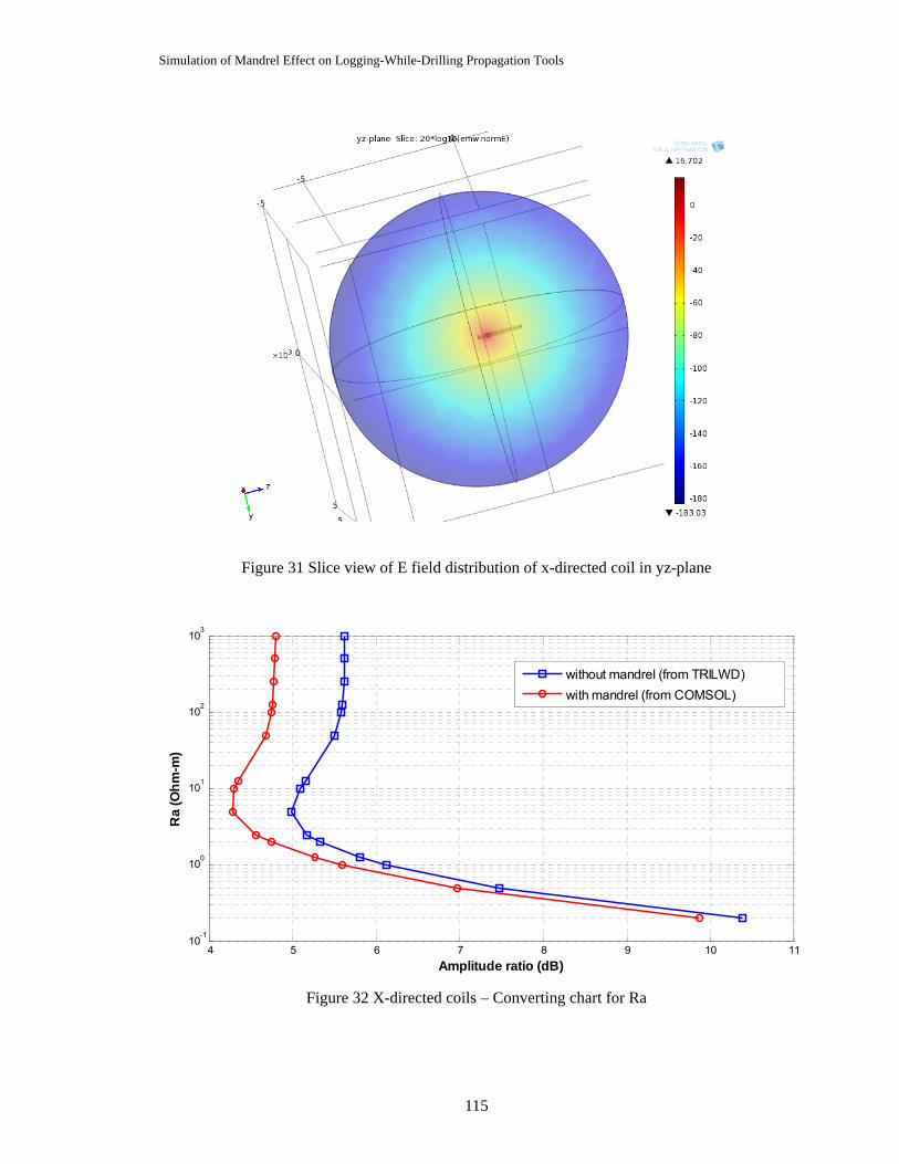
Simulation of Mandrel Effect on Logging-While-Drilling Propagation Tools
115
Figure 31 Slice view of E field distribution of x-directed coil in yz-plane
4 5 6 7 8 9 10 1110
-1
100
101
102
103
Ra
(Ohm
-m)
Amplitude ratio (dB)
without mandrel (from TRILWD)with mandrel (from COMSOL)
Figure 32 X-directed coils – Converting chart for Ra
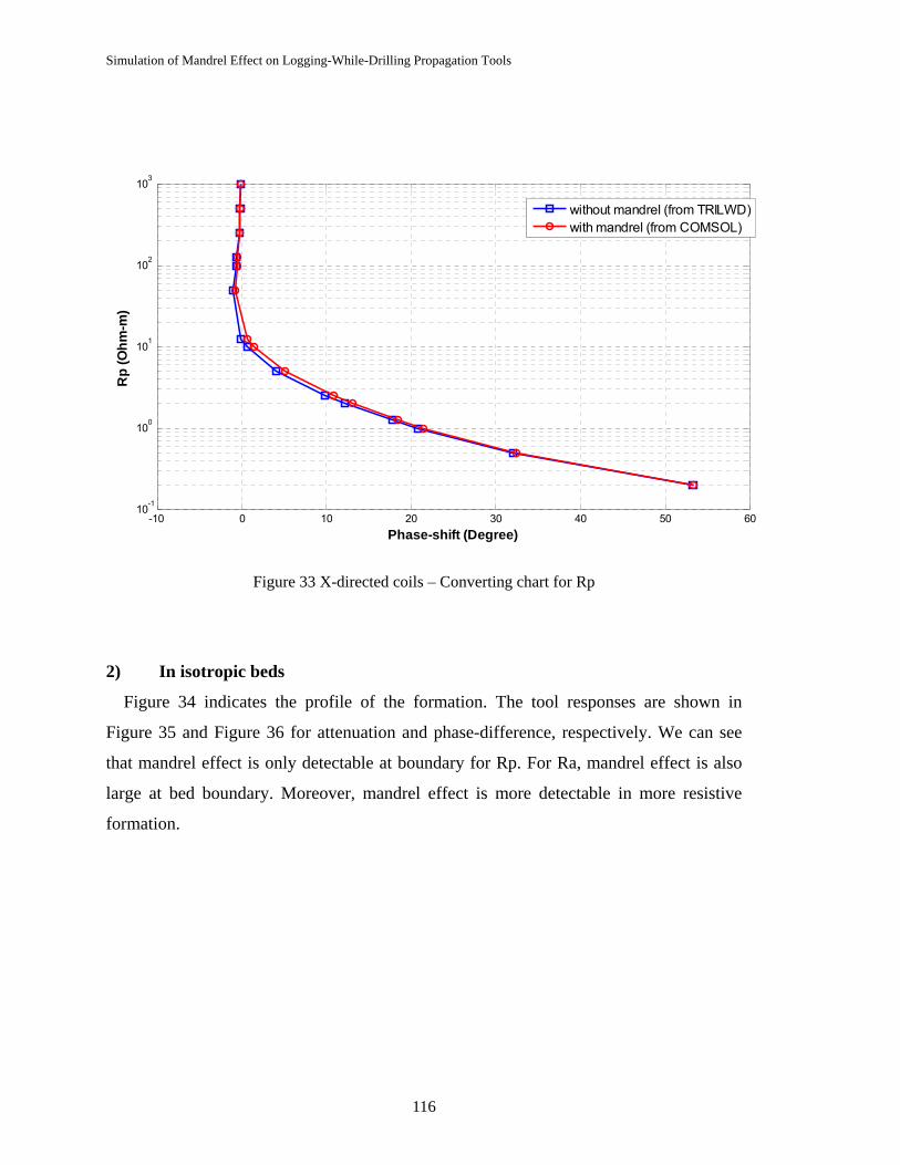
Simulation of Mandrel Effect on Logging-While-Drilling Propagation Tools
116
-10 0 10 20 30 40 50 6010-1
100
101
102
103
Rp
(Ohm
-m)
Phase-shift (Degree)
without mandrel (from TRILWD)with mandrel (from COMSOL)
Figure 33 X-directed coils – Converting chart for Rp
2) In isotropic beds
Figure 34 indicates the profile of the formation. The tool responses are shown in
Figure 35 and Figure 36 for attenuation and phase-difference, respectively. We can see
that mandrel effect is only detectable at boundary for Rp. For Ra, mandrel effect is also
large at bed boundary. Moreover, mandrel effect is more detectable in more resistive
formation.
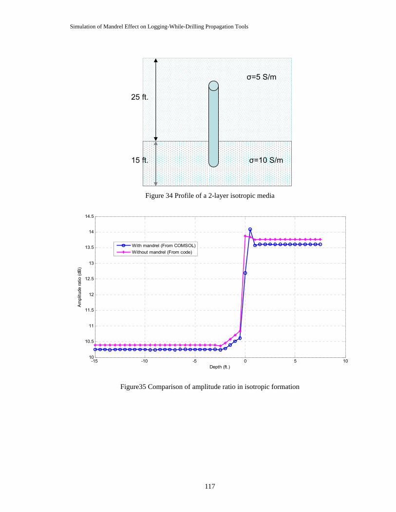
Simulation of Mandrel Effect on Logging-While-Drilling Propagation Tools
117
Figure 34 Profile of a 2-layer isotropic media
-15 -10 -5 0 5 1010
10.5
11
11.5
12
12.5
13
13.5
14
14.5
Depth (ft.)
Am
plitu
de ra
tio (d
B)
With mandrel (From COMSOL)Without mandrel (From code)
Figure35 Comparison of amplitude ratio in isotropic formation
σ=5 S/m
σ=10 S/m
25 ft.
15 ft.

Simulation of Mandrel Effect on Logging-While-Drilling Propagation Tools
118
-15 -10 -5 0 5 1050
55
60
65
70
75
80
Pha
se s
hift
(deg
ree)
Depth (ft.)
With mandrel (From COMSOL)Without mandrel (From code)
Figure 36 Comparison of phase-shift in isotropic formation
3) In anisotropic beds
We investigate the response of the x-directed coils only in vertical well because we
need to analyze the effect only contributed by anisotropy. We define phase-shift and
attenuation for the x-directed coils exactly the same way as for the z-directed coils. The
profile of formation is in rendered in Figure 37. The attenuation and phase-shift are
shown in Figure 38 and Figure 39, respectively. We can see that the difference caused by
mandrel in anisotropic formation is much the same as that in isotropic formation. We can
also observe that the x-directed coil system detects very little effect of anisotropy. The
converted logs, shown in Figure 40-41, read much the same as the resistivity of
horizontal direction.

Simulation of Mandrel Effect on Logging-While-Drilling Propagation Tools
119
Figure 37 Profile of formation
-15 -10 -5 0 5 105
5.2
5.4
5.6
5.8
6
6.2
6.4
6.6
6.8
7
Depth (ft.)
Am
plitu
de ra
tio (d
B)
With mandrel (From COMSOL)Without mandrel (From code)
Figure 18 Comparison of amplitude ratio in anisotropic formation
σv=0.1 S/m
25 ft.
20 ft.
σh=1 S/m
σv=0.2 S/m
σh=1 S/m

Simulation of Mandrel Effect on Logging-While-Drilling Propagation Tools
120
-15 -10 -5 0 5 1019
19.2
19.4
19.6
19.8
20
20.2
20.4
20.6
20.8
21
Phas
e sh
ift (d
egre
e)
Depth (ft.)
With mandrel (From COMSOL)Without mandrel (From code)
Figure 39 Comparison of phase-shift in anisotropic formation
-15 -10 -5 0 5 1010-1
100
101
Ra
(Ohm
-m)
Depth (ft.)
With mandrel (From COMSOL)Without mandrel (From TRILWD)RthRtv
Figure 40 Ra logs of dipole model and model with mandrel

Simulation of Mandrel Effect on Logging-While-Drilling Propagation Tools
121
-15 -10 -5 0 5 1010
0
101
Rp
(Ohm
-m)
Depth (ft.)
With mandrel (From COMSOL)Without mandrel (From TRILWD)RthRtv
Figure 41 Rp logs of dipole model and model with mandrel
4. Summary and conclusions
To get a full picture of the mandrel effect in LWD resistivity tools, dipole model and
model of finite size loop with mandrel have been used to simulate the tool response in
various types of formation. Two types of measurement are included in this thesis: one
with magnetic moment of coils pointed in the normal direction (z direction) of the beds,
the other with magnetic moment of coils pointed in the horizontal direction (x-direction)
of the beds.
Z-directed coils. In homogeneous media, results indicate that attenuation of dipole
model and mandrel model has about 0.5 dB shift, but the difference in phase shift is not
significant. In isotropic layered formation, Ra and Rp readings are only affected by the
presence of mandrel near the boundary. In anisotropic layered dipping beds, Ra and Rp
can be affected not only near the boundary but also the region far away form boundary.
The difference in Ra and Rp caused by mandrel is larger in the anisotropic formation
with higher anisotropy ratio.

Simulation of Mandrel Effect on Logging-While-Drilling Propagation Tools
122
X-directed coils. In homogeneous medium, we can see that mandrel also affects more
in Ra response than Rp for x-directed coils, similar to the z-directed coils. The conversion
chart for Ra and Rp become double valued. This will present difficulty when conversion
from phase-shift and attenuation to resistivity is needed. In isotropic layered formation,
the mandrel effect is obvious near the boundary. In anisotropic formation, the presence of
the mandrel can cause difference in Ra and Rp readings, but the effect is smaller than
what is seen with the z-directed coils.
Since in practice z-directed coil and x-directed coil are often combined to detect
boundary or anisotropy, we will present more results of combined coil system in the
future. With the confidence we gained on the COMSOL modeling of LWD propagation
tools, study of 3D effects will be further explored in the future.

Simulation of Mandrel Effect on Logging-While-Drilling Propagation Tools
123
Acknowledgement
The authors want to thank Dr. Minerbo of Schlumberger for his guidance on COMSOL.
We also appreciate KMSTechnologies for the donation of COMSOL software and the
computer. We thank all the Well Logging Industrial Consortium members for their
financial support.

Simulation of Mandrel Effect on Logging-While-Drilling Propagation Tools
124
References
[1] Dan Coope, Liang C. Shen and Frank S. C. Huang, “The Theory of 2 MHz
Resistivity Tool and Its Application to Measurement-While-Drilling,” The Log
Analyst, Vol. XXV, No. 3, May-June 1984, pp. 35-46.
[2] Brain Clark, Martin G. Liiling, Jacques Jundt, Mike Ross, and David Best, “A Dual
Depth Resistivity Measurement for FEWD,” 29th Annual Logging Symposium,
SPWLA, 1988.
[3] Terry Hagiwara, Erik J. Banning, Richard M. Ostermeier and S. Mark Haugland,
“Effects of Mandrel, Borehole, and Invasion for Tilt-Coil Antennas,” SPE ATCE,
Denver, CO, October 2003.
[4] Jian Yang, Dzevat Omeragic, Chengbing Liu, Qiming Li, Jan Smits, and Mike
Wilson, “Bed-Boundary Effect Removal to Aid Formation Resistivity Interpretation
from LWD Propagation Measurements at All Dip Angles,” 46th Annual Logging
Symposium, SPWLA, 2005.
[5] Self-learning Module, “Logging While Drilling (Geosteering Applications),”
TRACS INTERNATIONAL.
[6] John Zhou, “LWD/MWD Resistivity Tool Parameters,” Maxwell Dynamics, 2010.
[7] J. H. Moran and S. Gianzero, "Effects of formation anisotropy on resistivity-
logging measurements," Geophysics, vol. 44, no.7, pp. 1266-1286, July 1979.
[8] Ning Yuan, Zhijuan Zhang and Richard Liu, “Responses of Triaxial Induction
Tools in 1-D Multi-Layered Transverse Isotropic Formations,” Well Logging
Laboratory Technical Report No. 30, University of Houston, Chapter 2, 2009.
[9] L. L. Zhong, Simulation of Tri-axial Induction Tools in Dipping Anisotropic Beds,
Ph.D. dissertation, University of Houston, pp. 23-42, 2004.
[10] Zhijuan Zhang, 1D Modeling and Inversion of Triaxial Induction Logging Tool in
Layered Anisotropic Medium, Ph.D. dissertation, University of Houston, pp. 14-15,
2011.

Simulation of Mandrel Effect on Logging-While-Drilling Propagation Tools
125
[11] L. C. Shen, “Theory of Induction and MWD Tools in Cylindrically Layered
Medium,” Well Logging Laboratory Technical Report No.14, University of
Houston, Chapter 4, 1993
[12] Gerald Minerbo, Private Communication, August 2011
[13] Keli Sun, Dzevat Omeragic, Chanh Cao Minh, John Rasmus, Jian Yang, Andrei
Davydychev, Tarek Habashy, Roger Griffiths, Graham Reaper, and Qiming Li,
“Evaluation of Resistivity Anisotropy and Formation Dip from Directional
Electromagnetic Tools While Drilling,” 51st Annual Logging Symposium, SPWLA,
2010

Fast Finite-Difference Time-Domain Modeling for Marine-Subsurface Electromagnetic Problems using Artificially
High Dielectric Constant
126
CHAPTER 4
Fast Finite-Difference Time-Domain Modeling for
Marine-Subsurface Electromagnetic Problems using
Artificially High Dielectric Constant
Abstract
Finite-difference time-domain (FDTD) method was proposed by Yee in 1966 and
becomes one of the most popular numerical methods. It has been widely used in various
areas especially in electromagnetic (EM) modeling. In some areas such as sea-bed
logging, EM problems in marine-subsurface, ultra low frequency (ULF) is used and the
FDTD method will require extremely large number of time steps to get convergent results.
Thus, how to significantly reduce the large time-steps is essential for FDTD applications
in ULF problems. In this paper, we use an artificially high dielectric constant technique in
the FDTD simulation. The resultant method can obtain satisfying results with much less
time-steps than the original method. Numerical Examples will be presented to
demonstrate the capability of the present method.
1. Introduction
The finite-difference time-domain (FDTD) method was introduced by Yee in 1966 to
solve partial difference equation. It has become one of the primary available
computational electrodynamics modeling techniques and is widely used in various areas.
Since it is a time-domain method, FDTD solutions can cover a wide frequency range with
a single simulation run, and treat nonlinear material properties in a natural way.
Marine controlled-source has been under survey for many years, especially for
geophysical investigations. One particular application, called seabed logging, was

Fast Finite-Difference Time-Domain Modeling for Marine-Subsurface Electromagnetic Problems using Artificially
High Dielectric Constant
127
introduced by Eidesmo et al. and Ellingsrud et al. [2, 4] for offshore hydrocarbon
exploration. In this method, several receivers are set in different positions on the seabed.
The electric dipole which is transmitting electromagnetic wave is towing by a ship across
the seafloor and the receivers are recording electromagnetic waves in different positions
during towing. This method is often used to collect information of the sea bed to detect
hydrocarbon reservoirs. Hydrocarbon reservoirs are very resistive compared to the
sediments (the resistivity of the water-filled marine sediments is 1-5 Ohm-m) around
them.
In this paper, we are trying to use the FDTD method to deal with the EM problems in
marine-subsurface. As we know, the computation speed of a numerical solution is very
important for engineering and real-time problem solving..There are a lot of ways to
increase the speed of the FDTD algorithm such as the perfect matched layers (PML), up
scaling of artificially high electric permittivity. Both techniques have been implemented
in the FDTD solution in this paper.
PML was introduced by Berenger [1]. It is a method that can model an infinite large
solution domain by using the reflectionless boundaries in wave equations. That means
when the wave is propagating towards and reaches the PML boundary, there is no
reflection wave coming back to the solution domain. By introducing and implementing
the PML boundary, the solution domain is truncated and thus yields much less unknowns
in the FDTD simulation. Based on the Berenger’ PML, many new boundaries such as the
uniaxial PML, convolution PML etc. have been developed and proved to be more
efficient to more general media such as conductive media, dispersive media etc..
Up scaling of artificially high electric permittivity is used when the frequency is
extremely low like in sea bed logging. This method was introduced by Oristaglio and
Hohmann (1984) in [5] for modeling the transient response in 2D conductive earth
models. The main contribution is the introduction of an artificially high electric

Fast Finite-Difference Time-Domain Modeling for Marine-Subsurface Electromagnetic Problems using Artificially
High Dielectric Constant
128
permittivity. This method shows that in the case of extreme low frequency, we can
increase the value of the electric permittivity without changing the solution much. One
should note that the increase of the electric permittivity should not violate the stability
conditions. It is an approximate method but it can really increase the computation speed
and save much time. Both of the two methods mentioned above make the modeling of sea
bed electromagnetic problems possible.
2. Theory
2.1 Maxwell’s equations
First, the Maxwell’s equations are as follows
( )ij t ij j ijk j k iE H Jε σ δ∂ + = ∂ − (1)
t i ijk j k iH E Mμ δ∂ = − ∂ − (2)
ijkδ is the Levi-Civita tenosr. ijε is the electric permittivity tensor, ijσ is the
conductivity tensor. The j components of the electric and magnetic fields are kE and kH .
iJ and iM are the i-components of the electric and magnetic sources. μ is the
magnetic permeability which is assumed constant and equal to 74 10π −× H/m.
The Fourier transforms of the Maxwell’s equations from time to angular frequency
yields:
( )ij ij j ijk j k iE H Jιωε σ δ− + = ∂ − (3)
i ijk j k iH E Mιωμ δ− = − ∂ − (4)
As mentioned before, in sea-bed logging, the working frequency is usually as low as
0~10 Hz. In this situation, we notice that ijιωε− is much smaller than ijσ . To some
extent, we can increase ijε so that the total simulation time will decrease. It should be

Fast Finite-Difference Time-Domain Modeling for Marine-Subsurface Electromagnetic Problems using Artificially
High Dielectric Constant
129
noted that the increased ijε must still follow the condition that ij ijιωε σ− << .
2.2 Methodology of the 3D FDTD
The FDTD method starts from the Maxwell’s time-domain Equations.
DH Jt
∂∇× = +
∂ (5)
BE Mt
∂∇× = − −
∂ (6)
where E is the electric field, D is the displacement vector, H is the magnetic field
strength vector, B is the magnetic flux density vector, J is the electric current density
and M is the magnetic current density.
For linear, isotropic, and non-dispersive materials, there are
D Eε= (7)
B Hμ= (8)
where ε , μ are the electric permittivity and magnetic permeability of the material.
In FDTD algorithm, the solution domain is discretized into a lot of small grids. The E
and H field in every gird are calculated one by one. Fig. 1 shows the Yee grid used in this
papar. The electric field components are defined at the centers of the edges of the Yee
cells and oriented parallel to the respective edges while the magnetic field vector
components are defined at the centers of the faces of the Yee cells and are oriented
normal to the respective faces. This provides a simple picture of three-dimensional space
being filled by an interlinked array of Faraday’s law and Ampere’s law contours. The
material parameters of the Yee grid is shown in Fig.2.
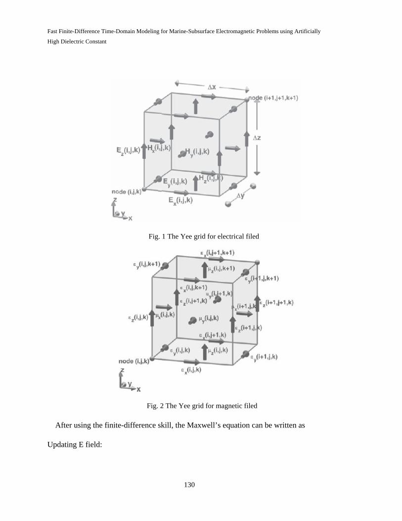
Fast Finite-Difference Time-Domain Modeling for Marine-Subsurface Electromagnetic Problems using Artificially
High Dielectric Constant
130
Fig. 1 The Yee grid for electrical filed
Fig. 2 The Yee grid for magnetic filed
After using the finite-difference skill, the Maxwell’s equation can be written as
Updating E field:

Fast Finite-Difference Time-Domain Modeling for Marine-Subsurface Electromagnetic Problems using Artificially
High Dielectric Constant
131
1( , , ) ( , , ) ( , , )n nx exe xE i j k C i j k E i j k+ = ×
1/2 1/2( , , ) ( ( , , ) ( , 1, ))n nexbz z zC i j k H i j k H i j k+ ++ × − −
1/2 1/2( , , ) ( ( , , ) ( , , 1))n nexby y yC i j k H i j k H i j k+ ++ × − −
1/2( , , ) ( , , )nexj ixC i j k J i j k++ × (9)
Where:
2 ( , , ) ( , , )( , , )2 ( , , ) ( , , )
2( , , )(2 ( , , ) ( , , ))
2( , , )(2 ( , , ) ( , , ))
2( , , )2 ( , , ) ( , , )
ex x
exe ex x
exbz ex x
exby ex x
exj ex x
i j k t i j kC i j ki j k t i j k
tC i j ki j k t i j k y
tC i j ki j k t i j k z
tC i j ki j k t i j k
ε σε σ
ε σ
ε σ
ε σ
−Δ=
+ ΔΔ
=+ Δ Δ
Δ= −
+ Δ Δ
Δ= −
+ Δ
1( , , ) ( , , ) ( , , )n ny eye yE i j k C i j k E i j k+ = ×
1/2 1/2( , , ) ( ( , , ) ( , , 1))n neybx x xC i j k H i j k H i j k+ ++ × − −
1/2 1/2( , , ) ( ( , , ) ( 1, , ))n neybz z zC i j k H i j k H i j k+ ++ × − −
1/2( , , ) ( , , )neyj iyC i j k J i j k++ × (10)
Where:
2 ( , , ) ( , , )( , , )
2 ( , , ) ( , , )
2( , , )(2 ( , , ) ( , , ))
2( , , )(2 ( , , ) ( , , ))
2( , , )2 ( , , ) ( , , )
ey y
eye ey y
eybx ey y
eybz ey y
eyj ey y
i j k t i j kC i j k
i j k t i j k
tC i j ki j k t i j k z
tC i j ki j k t i j k x
tC i j ki j k t i j k
ε σε σ
ε σ
ε σ
ε σ
−Δ=
+ Δ
Δ=
+ Δ Δ
Δ= −
+ Δ Δ
Δ= −
+ Δ

Fast Finite-Difference Time-Domain Modeling for Marine-Subsurface Electromagnetic Problems using Artificially
High Dielectric Constant
132
1( , , ) ( , , ) ( , , )n nz eze zE i j k C i j k E i j k+ = ×
1/2 1/2( , , ) ( ( , , ) ( 1, , ))n nezby y yC i j k H i j k H i j k+ ++ × − −
1/2 1/2( , , ) ( ( , , ) ( , 1, ))n nezbx x xC i j k H i j k H i j k+ ++ × − −
1/2( , , ) ( , , )nezj izC i j k J i j k++ × (11)
Where:
2 ( , , ) ( , , )( , , )2 ( , , ) ( , , )
2( , , )(2 ( , , ) ( , , ))
2( , , )(2 ( , , ) ( , , ))
2( , , )2 ( , , ) ( , , )
ez z
eze ez z
ezby ez z
ezbx ez z
ezj ez z
i j k t i j kC i j ki j k t i j k
tC i j ki j k t i j k x
tC i j ki j k t i j k y
tC i j ki j k t i j k
ε σε σ
ε σ
ε σ
ε σ
−Δ=
+ ΔΔ
=+ Δ Δ
Δ= −
+ Δ ΔΔ
= −+ Δ
Updating H field:
1 1/2( , , ) ( , , ) ( , , )n nx bxb xH i j k C i j k H i j k+ −= ×
( , , ) ( ( , , 1) ( , , ))n nbxey y yC i j k E i j k E i j k+ × + −
( , , ) ( ( , 1, ) ( , , ))n nbxez z zC i j k E i j k E i j k+ × + −
x( , , ) ( , , )nbxm iC i j k M i j k+ × (12)
Where

Fast Finite-Difference Time-Domain Modeling for Marine-Subsurface Electromagnetic Problems using Artificially
High Dielectric Constant
133
2 ( , , ) ( , , )( , , )2 ( , , ) ( , , )
2( , , )(2 ( , , ) ( , , ))
2( , , )(2 ( , , ) ( , , ))
2( , , )2 ( , , ) ( , , )
mx x
bxb mx x
bxey mx x
bxez mx x
bxm mx x
i j k t i j kC i j ki j k t i j k
tC i j ki j k t i j k z
tC i j ki j k t i j k y
tC i j ki j k t i j k
μ σμ σ
μ σ
μ σ
μ σ
−Δ=
+ ΔΔ
=+ Δ Δ
Δ= −
+ Δ Δ
Δ= −
+ Δ
1 1/2( , , ) ( , , ) ( , , )n ny byb yH i j k C i j k H i j k+ −= ×
( , , ) ( ( 1, , ) ( , , ))n nbyez z zC i j k E i j k E i j k+ × + −
( , , ) ( ( , , 1) ( , , ))n nbyex x xC i j k E i j k E i j k+ × + −
( , , ) ( , , )nbym iyC i j k M i j k+ × (13)
Where
2 ( , , ) ( , , )( , , )
2 ( , , ) ( , , )
2( , , )(2 ( , , ) ( , , ))
2( , , )(2 ( , , ) ( , , ))
2( , , )2 ( , , ) ( , , )
my y
bxb my y
byez my y
byex my y
bym my y
i j k t i j kC i j k
i j k t i j k
tC i j ki j k t i j k x
tC i j ki j k t i j k z
tC i j ki j k t i j k
μ σμ σ
μ σ
μ σ
μ σ
−Δ=
+ Δ
Δ=
+ Δ Δ
Δ= −
+ Δ Δ
Δ= −
+ Δ
1 1/2( , , ) ( , , ) ( , , )n nz bzb zH i j k C i j k H i j k+ −= ×
( , , ) ( ( , 1, ) ( , , ))n nbzex x xC i j k E i j k E i j k+ × + −
( , , ) ( ( 1, , ) ( , , ))n nbzey y yC i j k E i j k E i j k+ × + −
z( , , ) ( , , )nbzm iC i j k M i j k+ × (14)

Fast Finite-Difference Time-Domain Modeling for Marine-Subsurface Electromagnetic Problems using Artificially
High Dielectric Constant
134
Where:
2 ( , , ) ( , , )( , , )2 ( , , ) ( , , )
2( , , )(2 ( , , ) ( , , ))
2( , , )(2 ( , , ) ( , , ))
2( , , )2 ( , , ) ( , , )
mz z
bzb mz z
bzex mz z
bzey mz z
bzm mz z
i j k t i j kC i j ki j k t i j k
tC i j ki j k t i j k x
tC i j ki j k t i j k y
tC i j ki j k t i j k
μ σμ σ
μ σ
μ σ
μ σ
−Δ=
+ ΔΔ
=+ Δ Δ
Δ= −
+ Δ ΔΔ
= −+ Δ
As a summary, we can use a flow chart in Fig.2 to illustrate the steps of the FDTD
algorithm.

Fast Finite-Difference Time-Domain Modeling for Marine-Subsurface Electromagnetic Problems using Artificially
High Dielectric Constant
135
Fig.3 The flowchart of the FDTD algorithm
2.3 Material Approximations
When using the FDTD to solve the Maxwell’s equation, if the solution domain is a
homogenous medium, we just need to assign a value to iε , iσ and iμ , miσ . However,
in most cases, the media are inhomogeneous. Then, the average skill which take some
approximation strategies need to be applied.
In this report, the problem space is divided into a lot of grids which has unique

Fast Finite-Difference Time-Domain Modeling for Marine-Subsurface Electromagnetic Problems using Artificially
High Dielectric Constant
136
dimensions in the x-,y-, and z- direction. By using the averaging skill, the material
parameters iε , iσ , iμ , and miσ can be calculated as follows
( , , ) ( , 1, ) ( 1, 1, ) ( 1, 1, )( , , )4
( , , ) ( , 1, ) ( 1, 1, ) ( 1, 1, )( , , )4
2 ( , , ) ( , , 1)( , , )( , , ) ( , , 1)
2 ( , , ) ( , , 1)( , , )(
i
i
i
m mmi m
i j k i j k i j k i j ki j k
i j k i j k i j k i j ki j k
i j k i j ki j ki j k i j k
i j k i j ki j ki
ε ε ε εε
σ σ σ σσ
μ μμμ μσ σσ
σ
+ − + − − + − −=
+ − + − − + − −=
× × −=
+ −
× × −=
, , ) ( , , 1)mj k i j kσ+ −
(15)
where i can be x,y,z representing different direction.
2.4 Conditions for FDTD method
In the FDTD method, the internal time-stepping is restricted by the ratio of the grid
spacing and the fastest propagation velocity, known as the Courant-Friedriechs-Lewy
stability condition for hyperbolic equations:
21,2,3
11
( )i i
tc
x=
Δ ≤
Δ∑ (16)
where tΔ is the time-stepping, ixΔ is the spatial grid size in direction i, and
1/c με= is the speed of light in the medium. If we increase the electric permittivity ijε ,
the speed of light will reduce. Thus the internal time-stepping is increased, which will
result in decrease in the total computational time-step.
For ixΔ , we usually choose ixΔ < wavelength/10 to get an accurate simulation
results.
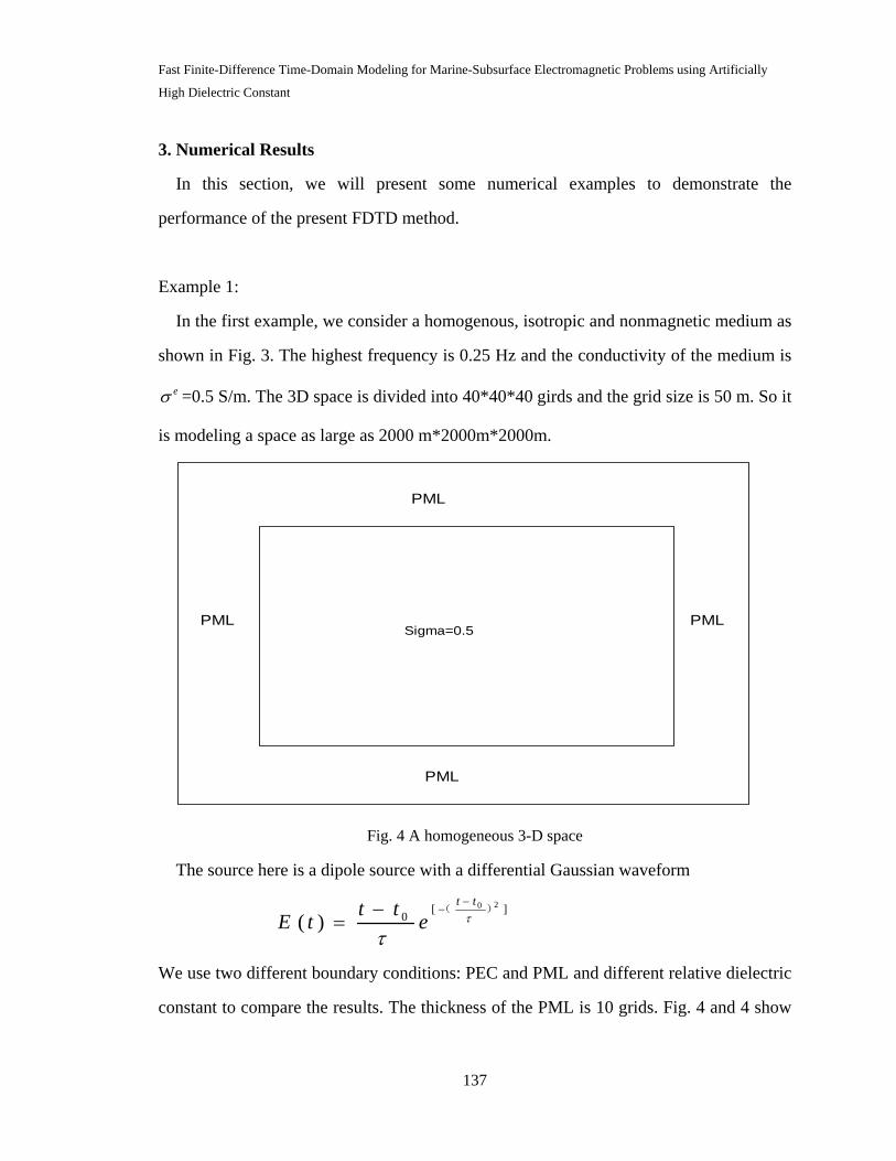
Fast Finite-Difference Time-Domain Modeling for Marine-Subsurface Electromagnetic Problems using Artificially
High Dielectric Constant
137
3. Numerical Results
In this section, we will present some numerical examples to demonstrate the
performance of the present FDTD method.
Example 1:
In the first example, we consider a homogenous, isotropic and nonmagnetic medium as
shown in Fig. 3. The highest frequency is 0.25 Hz and the conductivity of the medium is
eσ =0.5 S/m. The 3D space is divided into 40*40*40 girds and the grid size is 50 m. So it
is modeling a space as large as 2000 m*2000m*2000m.
PML
PML
PML
PMLSigma=0.5
Fig. 4 A homogeneous 3-D space
The source here is a dipole source with a differential Gaussian waveform
20[ ]0( )
t tt tE t e τ
τ
−−−
=( )
We use two different boundary conditions: PEC and PML and different relative dielectric
constant to compare the results. The thickness of the PML is 10 grids. Fig. 4 and 4 show

Fast Finite-Difference Time-Domain Modeling for Marine-Subsurface Electromagnetic Problems using Artificially
High Dielectric Constant
138
the results for different dielectric constant ( 49.6 10rε = × and 69.6 10rε = × ) when the
PEC boundary is used.
0 500 1000 1500 2000 2500 3000-10
-8
-6
-4
-2
0
2
4x 10⁻⁷
Timestep
mag
nitu
de E
x
Fig.5 The magnitude of Ex for 49.6 10rε = ×
( 5dt 2.685139170178605 10−= × , 47.234573839333053 10τ −= × )

Fast Finite-Difference Time-Domain Modeling for Marine-Subsurface Electromagnetic Problems using Artificially
High Dielectric Constant
139
0 100 200 300 400 500 600 700 800 900 1000-5
-4
-3
-2
-1
0
1
2x 10
-5
Timestep
mag
nitu
de E
x
Fig. 6 The magnitude of Ex for 69.6 10rε = ×
( 4dt 2.685139170178605 10−= × , 0.00723457383933τ = )
Fig. 6 and 7 show the calculated magnitude of Ex when using the PML boundary. The
transmitter position is at (22, 31, 31) and the receiver position is at (15, 31, 31).
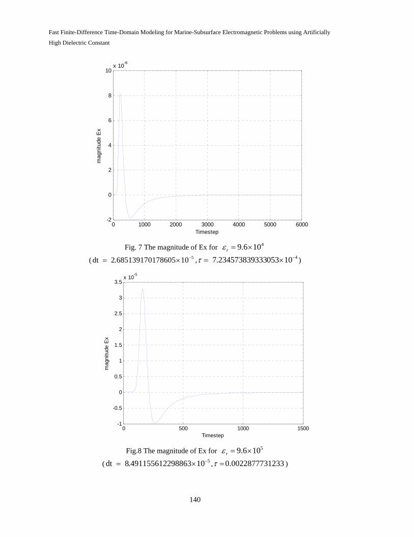
Fast Finite-Difference Time-Domain Modeling for Marine-Subsurface Electromagnetic Problems using Artificially
High Dielectric Constant
140
0 1000 2000 3000 4000 5000 6000-2
0
2
4
6
8
10x 10-6
Timestep
mag
nitu
de E
x
Fig. 7 The magnitude of Ex for 49.6 10rε = ×
( 5dt 2.685139170178605 10−= × , 47.234573839333053 10τ −= × )
0 500 1000 1500-1
-0.5
0
0.5
1
1.5
2
2.5
3
3.5x 10⁻⁵
Timestep
mag
nitu
de E
x
Fig.8 The magnitude of Ex for 59.6 10rε = ×
( 5dt 8.491155612298863 10−= × , 0.0022877731233τ = )

Fast Finite-Difference Time-Domain Modeling for Marine-Subsurface Electromagnetic Problems using Artificially
High Dielectric Constant
141
0 50 100 150 200 250 300 350 400 450 500-4
-3
-2
-1
0
1
2x 10
-5
Timestep
mag
nitu
de E
x
Fig.9 The magnitude of Ex for 89.6 10rε = ×
( dt 0.00268513917018= , 0.07234573839333τ = )
0 50 100 150 200 250 300 350 400-8
-6
-4
-2
0
2
4
6
8x 10⁻⁴
Timestep
mag
nitu
de E
x
Fig.10 The magnitude of Ex for 89.6 10rε = ×
( dt 0.00268513917018= , 0.07234573839333τ = )
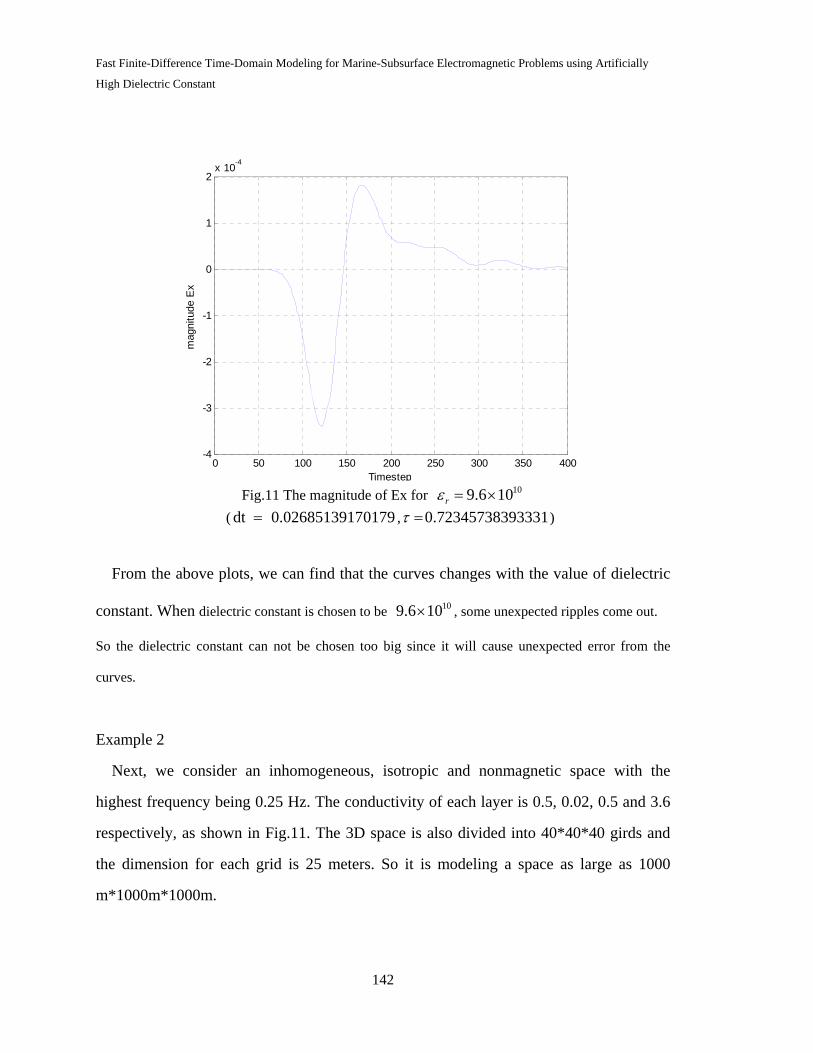
Fast Finite-Difference Time-Domain Modeling for Marine-Subsurface Electromagnetic Problems using Artificially
High Dielectric Constant
142
0 50 100 150 200 250 300 350 400-4
-3
-2
-1
0
1
2x 10⁻⁴
Timestep
mag
nitu
de E
x
Fig.11 The magnitude of Ex for 109.6 10rε = ×
( dt 0.02685139170179= , 0.72345738393331τ = )
From the above plots, we can find that the curves changes with the value of dielectric
constant. When dielectric constant is chosen to be 109.6 10× , some unexpected ripples come out.
So the dielectric constant can not be chosen too big since it will cause unexpected error from the
curves.
Example 2
Next, we consider an inhomogeneous, isotropic and nonmagnetic space with the
highest frequency being 0.25 Hz. The conductivity of each layer is 0.5, 0.02, 0.5 and 3.6
respectively, as shown in Fig.11. The 3D space is also divided into 40*40*40 girds and
the dimension for each grid is 25 meters. So it is modeling a space as large as 1000
m*1000m*1000m.
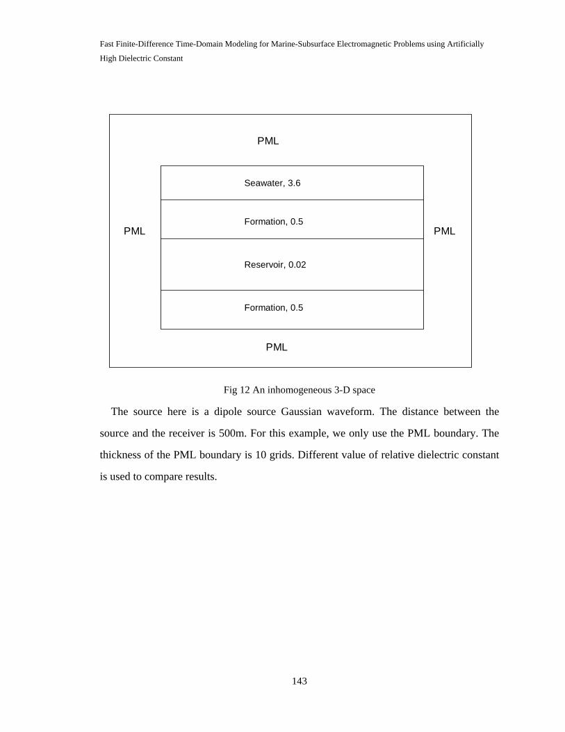
Fast Finite-Difference Time-Domain Modeling for Marine-Subsurface Electromagnetic Problems using Artificially
High Dielectric Constant
143
PML
PML
PML
PML
Seawater, 3.6
Formation, 0.5
Reservoir, 0.02
Formation, 0.5
Fig 12 An inhomogeneous 3-D space
The source here is a dipole source Gaussian waveform. The distance between the
source and the receiver is 500m. For this example, we only use the PML boundary. The
thickness of the PML boundary is 10 grids. Different value of relative dielectric constant
is used to compare results.
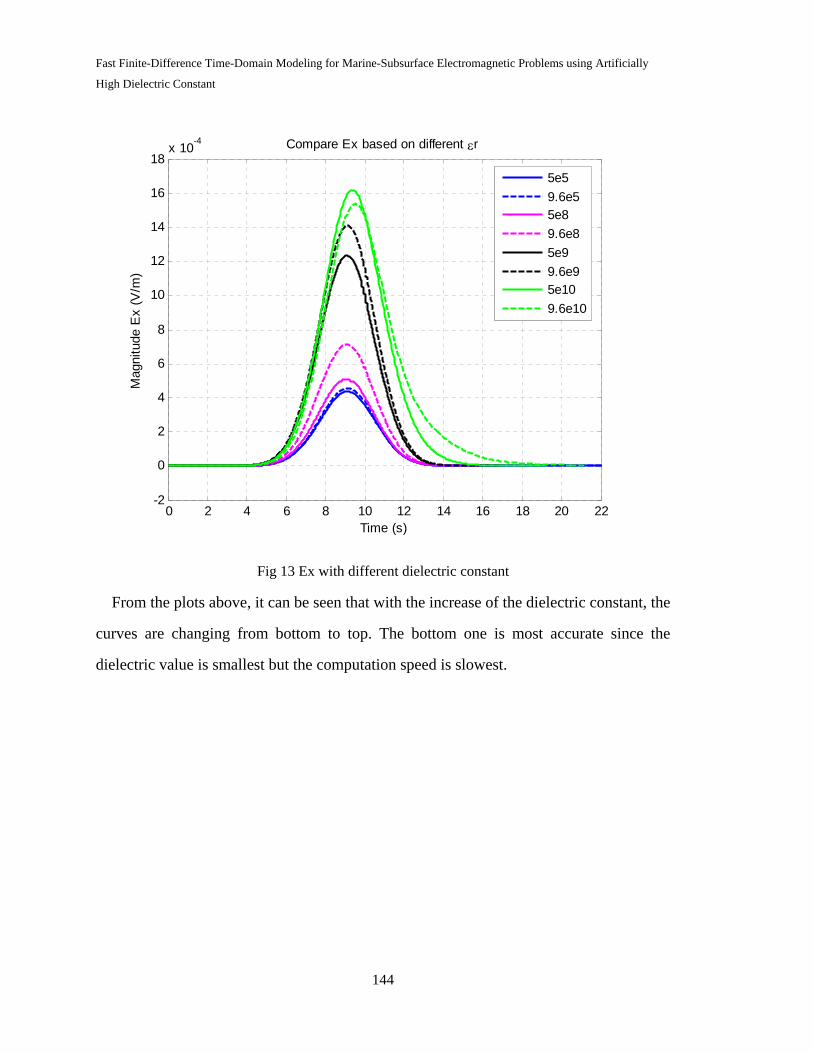
Fast Finite-Difference Time-Domain Modeling for Marine-Subsurface Electromagnetic Problems using Artificially
High Dielectric Constant
144
Fig 13 Ex with different dielectric constant
From the plots above, it can be seen that with the increase of the dielectric constant, the
curves are changing from bottom to top. The bottom one is most accurate since the
dielectric value is smallest but the computation speed is slowest.
0 2 4 6 8 10 12 14 16 18 20 22-2
0
2
4
6
8
10
12
14
16
18x 10-4
Time (s)
Mag
nitu
de E
x (V
/m)
Compare Ex based on different εr
5e59.6e55e89.6e85e99.6e95e109.6e10

Fast Finite-Difference Time-Domain Modeling for Marine-Subsurface Electromagnetic Problems using Artificially
High Dielectric Constant
145
Fig 14 Error analysis
From this plot, I compare the bottom two curves. It can be seen that those two are
almost overlap. The difference error which is calculated based on the peak value is less
than 4 percent, which is very acceptable.
4. Conclusion 61.3425695850893 10−×
This report looks into the ultra low frequency problem and introduces an method
(artificially high dielectric constant) to speed the computation. Speed of the EM waves is
affected by dielectric constant, which will change the total number of time step. However,
when the dielectric constant is increased artificially, it will reduce the accuracy of the
results. Error analysis is also done in order to have a deep look into this kind of low
frequency problem. So when the error is within an acceptable level, we can use this
method to improve the computation speed.
0 2 4 6 8 1 1 1 1 1 2 2-
0
2
4
6
8
1
1
1
1
1x
Time (s)
Magnitude
Compare Ex with different dielectric constant
5e5 9.6e5 5e8 9.6e8 5e9 9.6e9 5e10
9.6e10
Error <4%

Fast Finite-Difference Time-Domain Modeling for Marine-Subsurface Electromagnetic Problems using Artificially
High Dielectric Constant
146
References
[1] J.P. Berenger, “A perfectly matched layer for the absorbtion of electromagnetic
waves,” Journal of Computational Physics, vol.62, 185–200,1994
[2] T. Eidesmo, S. Ellingsrud ,L.M MacGregor, S. Constable, M. C. Sinha, S. Johansen,
F. N. Kong, and H. Westerdahl, “Sea bed logging SBL: a new method for remote
and direct identification of hydro carbon filled layers in deepwater areas: First
Break,” 20, 144–152, 2002.
[3] S. Ellingsrud, T. Eidesmo, S. Johansen, M. C. Sinha, L. M. MacGregor, and S.
Constable, “Remote sensing of hydrocarbon layers by seabed logging SBL: Results
from a cruise offshore Angola: The Leading Edge,” vol.21, 971–982,2002.
[4] A. M. Frank, “Fast finite-difference time-domain modeling for marine-subsurface
electromagnetic problems,” Geophysics, vol. 72, No.2 March April 2007;
P.A19-A23,
[5] M. L. Oristaglio and G. W. Hohmann, “Diffusion of electromagnetic fields into a
two-dimensional earth: A finite difference approach,” Geophysics, vol.49, 870–894,
1984
[6] T. Wang and G. W. Hohmann, “A finite-difference, time-domain solution for
three-dimensional electromagnetic modeling,” Geophysics, 58,797–809, 1993.
[7] The Finite Difference Time Domain Method for Electromagnetics: With MATLAB
Simulations Atef Elsherbeni (Author), Veysel Demir (Author)
[8] Computational Electrodynamics: The Finite-Difference Time-Domain Method, Third
Edition Allen Taflove (Author), Susan C. Hagness (Author)

New Addition and Modification to Well Logging Inversion Interface
147
CHAPTER 5
New Addition and Modification to Well Logging Inversion
Interface
Abstract
A new forward modeling CIND11 has been added to the Wellog Inversion Interface.
It is for simulation of induction tools in radial-layered formation. A new dialog has
been adopted in the interface for setting up radial-layered type formation. Moreover, a
module has been added to do one-dimensional calculation of AIT focusing tool
response. The forward model for LWD tool named LWD10 has been upgraded to take
care of multi-channel LWD tool calculation. The dialog for LWD tool creation also
upgraded for users to configure their own multi-channel LWD tools. The forward
LWDANI11 has been added to calculate response of multi-channel LWD tool in
anisotropic media. A simplified version of Wellog Inversion named Wellog Simulator
6.0 has been generated. Wellog Simulator has all the modules in Wellog Inversion for
simulation but no modules for inversion. Many other new added features and fixed
bugs will also be talked in this report.
1. New modeling codes added to the Interface
1.1 CIND11 code
CIND11 module is developed for calculating response of conventional induction
tools in radial-layered media. From inner to outer, the layers can be treated as mandrel,
borehole, invasion zones and formation. Number of regions should be no more than
99. The numerical integration accuracy is preset to be 0.01%. Due to the limitation of
the code, the conductivity of the mandrel material should not be very high. Otherwise,
user should switch to the corresponding module for LWD tool.

New Addition and Modification to Well Logging Inversion Interface
148
Figure 1 shows the new dialog for setting up radial-layered formation. It allows user
to define at most 99 layers in one formation file. Users can add or remove any layer
they want. Creating and editing function can be completed in this dialog. Note that the
first layer is treated as mandrel, so the outer radius should not be larger than the radii
of coils that defined in tool file. The default conductivity of mandrel has been set to
1e-6 S/m. If user wants to change it, be sure it is not very high.
Figure 1 Dialog for cylindrical-layered formation design
The result of CIND11 is essentially zero dimensional calculation, so it is displayed
in a list box as opposed to a log curve. An example result is shown in Figure 2. As we
can see, all the tool information and formation parameters will also be listed.

New Addition and Modification to Well Logging Inversion Interface
149
Figure 2 An example result of CIND11 module
1.2 AIT1D code
Previously, AIT tools can only be simulated in 2-D calculations because parameters
of AIT tools are confidential and they are only wrapped in a 2-D module. Now we add
a wrapper for induction 1-D calculation to provide AIT tools’ parameters so that the
module for conventional induction tools can also yield results for AIT tools. It is more
convenient for users to compare 1-D and 2-D calculations for AIT tools. Figure 3
shows 1-D and 2-D results of a 4-foot set AIT tool in Oklahoma formation. The
dipping angle is chosen to be zero.
Figure 3 1-D and 2-D comparison of a 4-foot set AIT tool

New Addition and Modification to Well Logging Inversion Interface
150
To have this AIT1D code also allows us to calculate tool response in dipping beds
which is not available in 2-D simulation. Figure 4 is the logs of a 2-foot set AIT tool
response in Oklahoma formation with a 70 degrees dip. We can see that the results
agree well with an early publication [2] which is rendered in Figure 5.
Figure 4 2-ft set AIT tool in Oklahoma formation with 70-degree dip (Wellog Inversion)
Figure 5 2-ft set AIT tool in Oklahoma formation with 70-degree dip (Barber, 2001)
1.3 Upgraded LWD10 code
Previously, LWD10 code can only calculate the response of a group of one
transmitter and two receivers (referred to as a channel) of a LWD tool at one time.
That means if a LWD tool has four channels, we need to define four different tool
files, and as a results we need to calculate four times to get all the response for this
tool. Now the upgraded LWD10 code can take care of multi-channel calculation
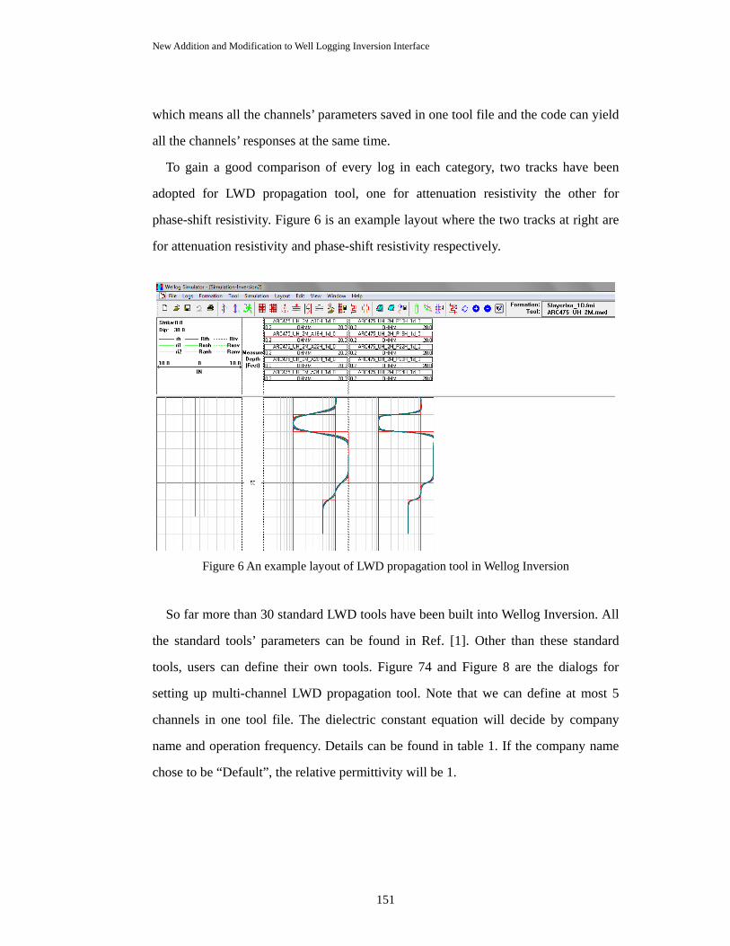
New Addition and Modification to Well Logging Inversion Interface
151
which means all the channels’ parameters saved in one tool file and the code can yield
all the channels’ responses at the same time.
To gain a good comparison of every log in each category, two tracks have been
adopted for LWD propagation tool, one for attenuation resistivity the other for
phase-shift resistivity. Figure 6 is an example layout where the two tracks at right are
for attenuation resistivity and phase-shift resistivity respectively.
Figure 6 An example layout of LWD propagation tool in Wellog Inversion
So far more than 30 standard LWD tools have been built into Wellog Inversion. All
the standard tools’ parameters can be found in Ref. [1]. Other than these standard
tools, users can define their own tools. Figure 74 and Figure 8 are the dialogs for
setting up multi-channel LWD propagation tool. Note that we can define at most 5
channels in one tool file. The dielectric constant equation will decide by company
name and operation frequency. Details can be found in table 1. If the company name
chose to be “Default”, the relative permittivity will be 1.

New Addition and Modification to Well Logging Inversion Interface
152
Figure 7 Dialog for LWD tool configuration
Figure 8 Dialog for LWD tool coils spacing setting
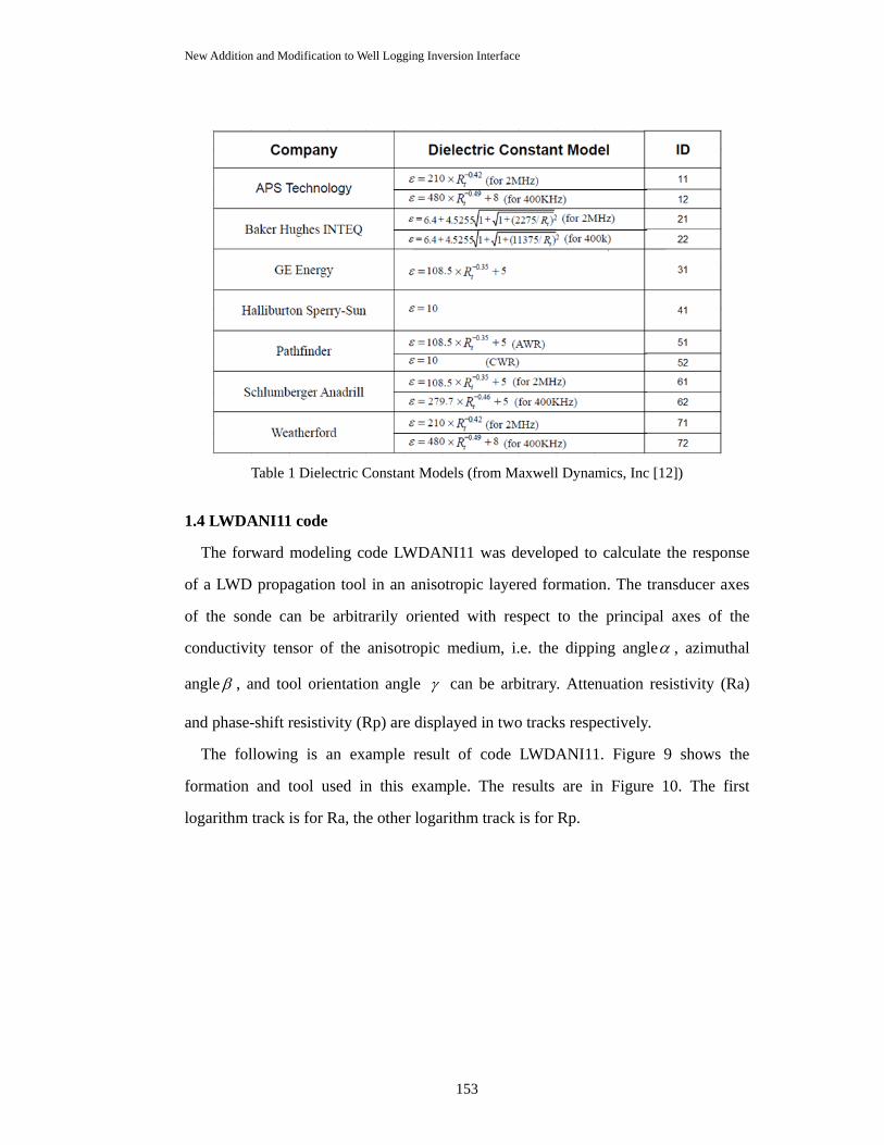
New Addition and Modification to Well Logging Inversion Interface
153
Table 1 Dielectric Constant Models (from Maxwell Dynamics, Inc [12])
1.4 LWDANI11 code
The forward modeling code LWDANI11 was developed to calculate the response
of a LWD propagation tool in an anisotropic layered formation. The transducer axes
of the sonde can be arbitrarily oriented with respect to the principal axes of the
conductivity tensor of the anisotropic medium, i.e. the dipping angleα , azimuthal
angle β , and tool orientation angle γ can be arbitrary. Attenuation resistivity (Ra)
and phase-shift resistivity (Rp) are displayed in two tracks respectively.
The following is an example result of code LWDANI11. Figure 9 shows the
formation and tool used in this example. The results are in Figure 10. The first
logarithm track is for Ra, the other logarithm track is for Rp.

New Addition and Modification to Well Logging Inversion Interface
154
Figure 9 Formation and tool information of the example
Figure 10 Example result of LWDANI11 code
2. Other improvements in the interface application
2.1 Different tracks for logs of different category
To gain a better view of layout and to make it easier for user to compare logs of
different category, we will automatically load logs of different category to different
tracks. For instance, we have two linear tracks for the results of TRITI09 code, one is
for H-field logs and the other is for apparent resistivity logs. For the results of LWD
tools, we have one logarithm track for logs of attenuation resistivity and the other for

New Addition and Modification to Well Logging Inversion Interface
155
logs of phase-shift resistivity.
2.2 Addition of select log dialog
Since there will be many curves in one track, it is not possible for users to view
each curve clearly. Now a submenu has been added to enable users select any curve or
several curves in a track to display at a time. Right clicking on the legend area of a
track, a list box will pop out as shown in Figure 11. The list box lists all the names of
logs belonged to this track. Click the names to select logs to be displayed. Figure 12
shows the layout of two selected logs, one in each track. The scale of each track will
automatically adjust with scales of all the selected logs. We can see that the layout
after selection is much clearer than the original one.
Figure 11 Dialog for select logs
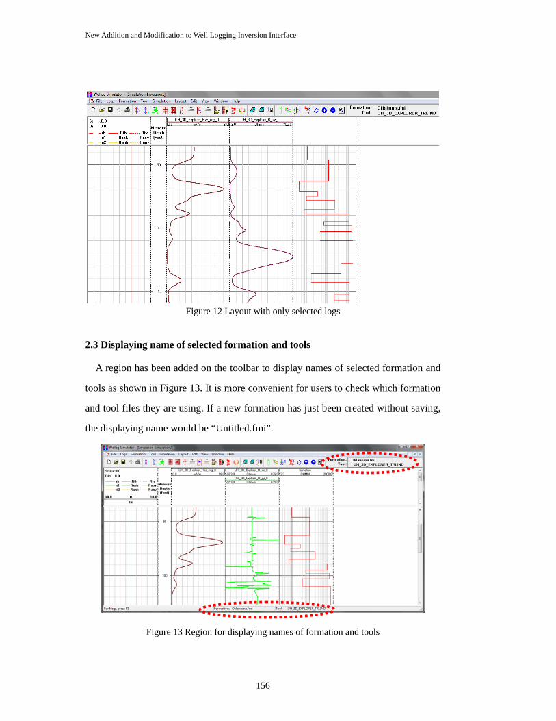
New Addition and Modification to Well Logging Inversion Interface
156
Figure 12 Layout with only selected logs
2.3 Displaying name of selected formation and tools
A region has been added on the toolbar to display names of selected formation and
tools as shown in Figure 13. It is more convenient for users to check which formation
and tool files they are using. If a new formation has just been created without saving,
the displaying name would be “Untitled.fmi”.
Figure 13 Region for displaying names of formation and tools
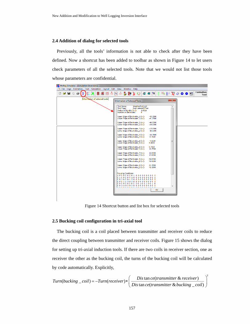
New Addition and Modification to Well Logging Inversion Interface
157
2.4 Addition of dialog for selected tools
Previously, all the tools’ information is not able to check after they have been
defined. Now a shortcut has been added to toolbar as shown in Figure 14 to let users
check parameters of all the selected tools. Note that we would not list those tools
whose parameters are confidential.
Figure 14 Shortcut button and list box for selected tools
2.5 Bucking coil configuration in tri-axial tool
The bucking coil is a coil placed between transmitter and receiver coils to reduce
the direct coupling between transmitter and receiver coils. Figure 15 shows the dialog
for setting up tri-axial induction tools. If there are two coils in receiver section, one as
receiver the other as the bucking coil, the turns of the bucking coil will be calculated
by code automatically. Explicitly, 3
tan ( & )( _ ) ( )tan ( & _ )
Dis ce transmitter receiverTurn bucking coil Turn receiverDis ce transmitter bucking coil
⎛ ⎞= − ∗⎜ ⎟
⎝ ⎠

New Addition and Modification to Well Logging Inversion Interface
158
Figure 15 Dialog for tri-axial tool configuration
2.6 Updating help file and manual
All error codes in the help file have been corrected. New additions and modifications
have been added to the help file and user manual.
2.7 Other fixed bugs in Wellog Inversion
1) Logging point restriction
In the old version, to avoid overflow in FORTRAN, Wellog Inversion had a limitation
on logging stop position to be no larger than 10,000 feet. It is not reasonable since
logging can be conducted at any depth. Now we have changed the restriction to the

New Addition and Modification to Well Logging Inversion Interface
159
maximum logging points to be 10,000.
2) Borehole compensated coil position
Previously, if the borehole compensated feature is checked, Wellog Inversion would
take the opposite value of original transmitter’s position as the compensated
transmitter’s position. It would be a problem if the middle point of the receiver pair is
not at zero. Now new algorithm has been adopted to calculate the transmitter’s
position.
3) Dialog for run simulation crashes a lot
If any mal-operation happened, there would pop out an error message which would
also disable the OK button. Even though the user made a right choice at last, the OK
button is still disabled. Now this bug has been fixed.
4) Larger length for log name when saving a log
In the old version, the string length for log name was not large enough and as a result
the log name was not complete when saving a log. Now we have made a larger string
length for log names. Also, a limitation has been made to the length of tool name so
that the log name would not exceed our expecting length.
5) Automatically calculate tool constant when saving laterolog tool file
Originally, when defining a laterolog tool, if user does not click “Calculate tool
constant” before saving the tool, the tool constant would save as default value
regardless of the tool’s configuration. Now interface will calculate the tool constant
automatically when saving the tool file.
3. Wellog Simulator 6.0

New Addition and Modification to Well Logging Inversion Interface
160
Wellog Simulator 6.0 is a simplified version of Wellog Inversion. It inherits all the
forward modeling modules in Wellog Inversion and removes all the inversion
modules. Wellog Simulator 6.0 intends to be a compact interface for 1D and 2D
simulation for all the induction, LWD and laterolog tools. No 3D module is integrated
to Wellog Simulator 6.0.
Wellog Simulator 6.0 requires users to select tool first. Formation selection or
creation is allowed only after tool selection. This enables the interface to lead users to
load proper formation for the tool they selected. For example, radial-layered
formation is not allowed to create or load if the selected tool is not conventional
induction tool. This makes sure that users do not waste their time.
Wellog Simulator 6.0 automatically checks all the allowed dimensions to calculate
after formation and tool selection. If user wants to do other dimensional calculation,
interface will give a reminder message and then automatically configure needed
parameters for the chosen calculation. For instance, if a 1D formation is defined, but
user wants to run 2D simulation, interface will remind user that it will automatically
give borehole radius, mud conductivity and parameters of invasion and then do the 2D
simulation.

New Addition and Modification to Well Logging Inversion Interface
161
References
[1] John Zhou, “LWD/MWD Resistivity Tool Parameters,” Maxwell Dynamics,
2010.
[2] Thomas D. Barber and Frank Shray, “Case Studies Using Advanced
Interpretation Techniques for Induction Logs,” SPE, 2001

Wireless Relay Network: Novel Data Transmission Approach for Measurement-While-Drilling Telemetry
162
CHAPTER 6
Wireless Relay Network: Novel Data Transmission Approach
for Measurement-While-Drilling Telemetry
Abstract
This project presents a novel downhole data transmission solution, Wireless Relay
Network (WRN), to facilitate data telemetry in measurement-while-drilling (MWD)
telemetry for oil and gas exploration. WRN includes the following key designs. First, we
use small form factor transceivers (nodes) to construct bi-directional, multihop wireless
links in the downhole environment. Second, we adopt an efficient hierarchical architecture
consisting of Basic Relay Nodes (BRN) and Routing Initiation Nodes (RIN): BRN simply
forwards packets to intended destinations, while RIN involves higher-level protocols such
as routing and error detection. Finally, we propose a network protocol including routing
and packet retransmission schemes to serve specific demands of WRN. Simulations with
different settings are conducted to demonstrate the feasibility of WRN. Modeling the
downhole MWD tools as a 1024 bps source, an overall throughput of 660 bps can be
reached over a 10,000-meter transmission distance. As a high-speed transmission method,
WRN can be a promising alternative to currently used data transmission techniques in the
oil industry.
1. Introduction
High-speed data transmission has long been a preferable feature of advanced
Measurement-While-Drilling (MWD) telemetry techniques in the oil and gas industry.
Various downhole information is collected by sensors during drilling process, including
directional parameters, drilling conditions, and formation characteristics. All the data are
storaged to be retrieved later to create a complete well log, while some are selected to be
transmitted to the surface in real time. Operator can thus instantly make optimal decisions
on drilling operation to maximize drilling efficiency and productivity, as well as to avoid

Wireless Relay Network: Novel Data Transmission Approach for Measurement-While-Drilling Telemetry
163
potential tool failures or subsurface accidents [1]. In some cases, it is also necessary to send
commands downward to control the bottom hole assembly tools. Therefore, a two-way
communication link is generally required.
The most widespread telemetry method used in current MWD systems is mud pulse
telemetry (MPT), designed by J. J. Arps in 1964 [2]. Using a controllable valve in the drill
collar, the pressure of drilling mud flow is modulated with a digital signal that can be
recovered at the surface. During the past few decades, MPT has been improved by using
advanced mud pulsers and data compression schemes [3]-[5], although the data rate is still
as low as 1-30 bps [6], [7], limited by its intrinsic mechanical features. Moreover, it does
not apply to certain circumstances such as underbalanced drilling, where the pressure of
drilling mud cannot be easily changed due to the presence of compressible inert gas
contents.
Another solution for data transmission from the bottom to the surface while drilling is
Electromagnetic Telemetry (EMT), which uses electromagnetic propagation through the
earth [8], [9]. By emanating a modulated signal from the borehole through the formations,
data can be sent up to the surface at a rate of up to 100 bps. Although EMT is a good
alternative to MPT in some cases, it is problematic in wells of great depth. Higher
frequency signal suffers severe attenuation through the conductive formations [10]-[12],
while low frequency signal is easily disturbed by seismic currents and other interference in
the earth. Both factors consequently lead to an extremely low signal-to-noise-ratio at the
receiver and therefore unreliable telemetry results.
To completely insulate the signal from environmental disturbance, a wired drill pipe
system, Intellipipe, was presented by Grant Prideco in 2003 [13]. Intellipipe uses
high-speed cables built in the drill pipe to accomplish a two-way communication link.
According to the field trial reports, a bandwidth of 57,000 bps can be achieved [14]-[17].
However, the whole technology is based on the specially-designed equipment including
adapted top drive and drillstring, which makes it expensive and non-adaptive. Another
disadvantage lies in the potential mechanical weakness of the system. Any damage to a
pipe joint can lead to a communication failure and increase downtime.
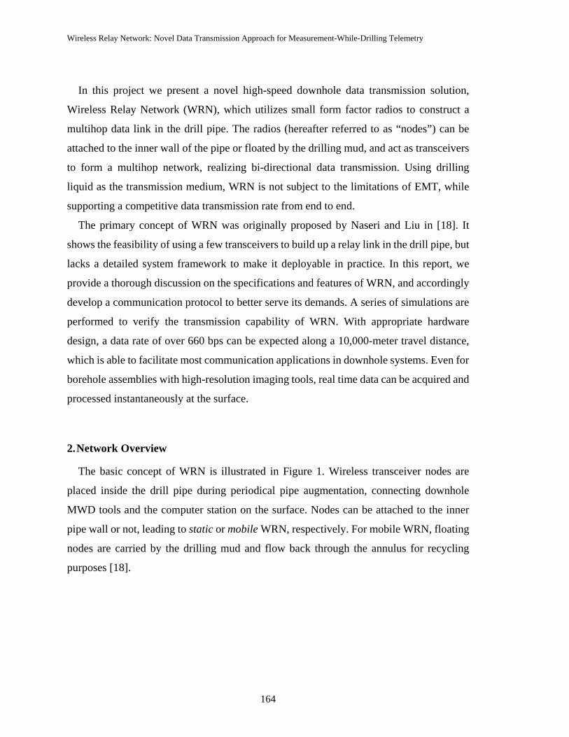
Wireless Relay Network: Novel Data Transmission Approach for Measurement-While-Drilling Telemetry
164
In this project we present a novel high-speed downhole data transmission solution,
Wireless Relay Network (WRN), which utilizes small form factor radios to construct a
multihop data link in the drill pipe. The radios (hereafter referred to as “nodes”) can be
attached to the inner wall of the pipe or floated by the drilling mud, and act as transceivers
to form a multihop network, realizing bi-directional data transmission. Using drilling
liquid as the transmission medium, WRN is not subject to the limitations of EMT, while
supporting a competitive data transmission rate from end to end.
The primary concept of WRN was originally proposed by Naseri and Liu in [18]. It
shows the feasibility of using a few transceivers to build up a relay link in the drill pipe, but
lacks a detailed system framework to make it deployable in practice. In this report, we
provide a thorough discussion on the specifications and features of WRN, and accordingly
develop a communication protocol to better serve its demands. A series of simulations are
performed to verify the transmission capability of WRN. With appropriate hardware
design, a data rate of over 660 bps can be expected along a 10,000-meter travel distance,
which is able to facilitate most communication applications in downhole systems. Even for
borehole assemblies with high-resolution imaging tools, real time data can be acquired and
processed instantaneously at the surface.
2. Network Overview
The basic concept of WRN is illustrated in Figure 1. Wireless transceiver nodes are
placed inside the drill pipe during periodical pipe augmentation, connecting downhole
MWD tools and the computer station on the surface. Nodes can be attached to the inner
pipe wall or not, leading to static or mobile WRN, respectively. For mobile WRN, floating
nodes are carried by the drilling mud and flow back through the annulus for recycling
purposes [18].
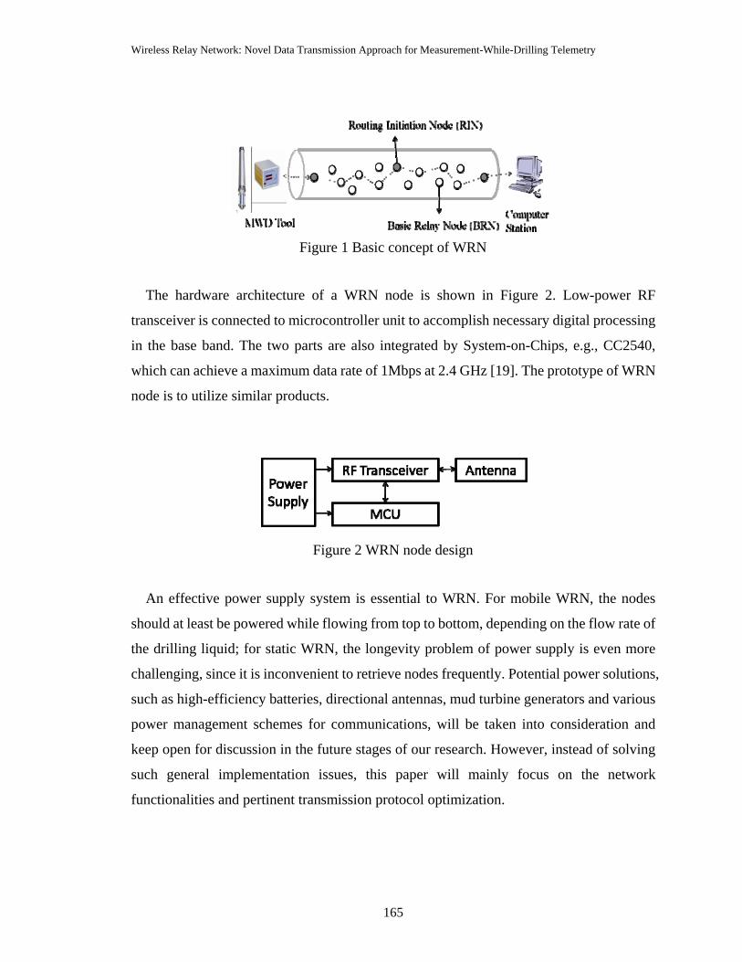
Wireless Relay Network: Novel Data Transmission Approach for Measurement-While-Drilling Telemetry
165
The hardware architecture of a WRN node is shown in Figure 2. Low-power RF
transceiver is connected to microcontroller unit to accomplish necessary digital processing
in the base band. The two parts are also integrated by System-on-Chips, e.g., CC2540,
which can achieve a maximum data rate of 1Mbps at 2.4 GHz [19]. The prototype of WRN
node is to utilize similar products.
An effective power supply system is essential to WRN. For mobile WRN, the nodes
should at least be powered while flowing from top to bottom, depending on the flow rate of
the drilling liquid; for static WRN, the longevity problem of power supply is even more
challenging, since it is inconvenient to retrieve nodes frequently. Potential power solutions,
such as high-efficiency batteries, directional antennas, mud turbine generators and various
power management schemes for communications, will be taken into consideration and
keep open for discussion in the future stages of our research. However, instead of solving
such general implementation issues, this paper will mainly focus on the network
functionalities and pertinent transmission protocol optimization.
Figure 2 WRN node design
Figure 1 Basic concept of WRN

Wireless Relay Network: Novel Data Transmission Approach for Measurement-While-Drilling Telemetry
166
As an ad-hoc wireless network, WRN for MWD telemetry has some distinguished features
that require special treatment to optimize the network performance:
High latency: WRN is a network with a single source node and a single destination
node at each end of the pipe, and a large number of intermediate relay nodes. According to
[18], a typical transmission range for a transceiver node in oil based mud is around 10
meters. This means for a 10,000-meter-long pipe, the minimum number of hops from end
to end is 1000. Assume a 20 ms processing delay is added in at each hop, it will take over
20 s to deliver a single data packet. Given such conditions, some of the prevalent
transmission schemes, like end-to-end packet acknowledgement, will simply become
impractical and have to be modified.
Periodically increased network scale: WRN is a self-expanded network. New nodes
are placed in with installation of every pipe section, thus the network size and span are
increasing regularly and periodically. This feature can be leveraged to improve network
performance. For example, since the network stays relatively static during the interval
between every two pipe installation operations, route information can be updated less
frequently to avoid unnecessary control overhead.
Reliability-oriented: Reliability is regarded as the top priority in WRN system. Since
the source data are generated continuously while drilling, data loss can be critical.
Therefore, error detection and/or correction and packet retransmission are necessary.
Moreover, in case of node loss, a certain amount of node density should be guaranteed, so
that the whole communication link would not be completely interrupted by a minor node
failure. This in turn imposes a tradeoff between signal-to-interference ratio and redundancy
on system design and protocol optimization.
In addition, WRN nodes are intended to be developed on relatively low-cost systems,
which usually have limited memory and processing capability. As a result, the
communication protocols of WRN should be light-weighted.

Wireless Relay Network: Novel Data Transmission Approach for Measurement-While-Drilling Telemetry
167
3. Network Hierarchy and Protocols
3.1 Network Hierarchy
Two types of nodes are defined in WRN: Basic Relay Nodes (BRN) and Routing
Initiation Nodes (RIN). RIN nodes are distributed equidistantly in the pipeline, while
multiple BRN nodes are placed between every two RIN nodes, as shown in Figure 1 and
Figure 3.
BRN nodes function as the most fundamental relay stations, forwarding data packets
until they reach the nearest RIN nodes. They do not generate or maintain any control
information.
RIN nodes involve higher layer functions such as routing and reliability management.
They act as bridges that connect two groups of BRN nodes from both sides. Local route
information is collected and updated by RIN nodes. They also perform data error detection
and request packet retransmissions to guarantee a reliable transmission.
The hierarchical architecture of WRN is designed to reduce control overhead and
processing latency. Considering about the extremely slim network structure of WRN, it is
unrealistic to acquire global information in a short time. With RIN nodes, the whole
network is divided into multiple subnets, inside which local network statistics can be easily
updated and handled. For example, instead of finding an end-to-end path, global route
information is broken into segments and stored at RIN nodes. In other words, an RIN node
only needs to know how to reach adjacent RIN nodes through a multihop BRN link. A
similar structure is used in [20].
Figure 3 WRN addressing

Wireless Relay Network: Novel Data Transmission Approach for Measurement-While-Drilling Telemetry
168
3.2 Routing
The addresses of RIN and BRN nodes are assigned separately. The two types of nodes
are differentiated by the last bit in addresses (RIN tag): 1 for an RIN node and 0 for a BRN
node.
RIN addresses are sequentially assigned from bottom to top. Since the relative depth
information is implied by addresses of RIN nodes, the directions of packet transmission
can be easily controlled. For example, for logging information that is supposed to be
transferred from MWD tool to the surface, RIN nodes will select specific routes that can
reach neighboring RIN nodes with larger RIN addresses instead of smaller ones.
BRN addresses are not strictly associated with location information but randomly
assigned in a certain range. In fact, BRN addresses can be spatially reused without
confusion. As shown in Figure 3, two groups of BRN addresses, 1-5 and 6-10, are used
reciprocally in the pipe. There will be no identification problems because RIN nodes only
collect local route information involving adjacent RINs, as mentioned above. Take the
address assignment in Figure 3 for an example, if appeared in a routing table of RIN 2, a
BRN 4 refers to the one located between RIN 2 and 1; but for RIN 3, BRN 4 is along the
path to RIN 4.
Since the topology of WRN remains relatively static during most time, a proactive
routing scheme is adopted, i.e., route discovery procedure is performed periodically
instead of on demand. First, each RIN node broadcasts a route request (RREQ). All nearby
BRN nodes forward this request until it reaches another RIN node, which immediately
sends back a route reply (RREP) with available route information. This information is then
kept in a routing table and updated if any route dynamics are detected. Since there could be
multiple paths between RIN nodes, the whole communication link will not be completely
broken due to any minor node loss.
The routing table consists of both upstream and downstream path information. When a
data packet arrives, the RIN node checks the direction of its destination, and selects a route
in the corresponding category. The used path is then set with an occupation flag for a
certain time cycle before it can be selected again.

Wireless Relay Network: Novel Data Transmission Approach for Measurement-While-Drilling Telemetry
169
3.3 Packet Retransmission
We use cyclic redundancy check (CRC), a simple but effective code for error detection
[21], because of its advantage to deal with burst errors which may happen frequently in
WRN.
As shown in Figure 4, when a data packet arrives at an RIN node, CRC is re-calculated
from the original data field and compared with the received value. If the check values
match, the receiver RIN will send back an acknowledgment (ACK) to the previous RIN,
and push the data packet to the buffer for transmission; otherwise it sends out a negative
acknowledgment (NACK) to request a retransmission. The number of retransmissions
cannot be higher than MAX_RETRANS, otherwise the data packet will be discarded.
Every data packet should be stored at the RIN after being transmitted. Without ACK or
NACK, a packet will be transmitted again along a different path.
4. Simulation
Simulations are performed to verify the feasibility of WRN. The main parameters are
Figure 4 Error detection algorithm

Wireless Relay Network: Novel Data Transmission Approach for Measurement-While-Drilling Telemetry
170
listed in Table 1. Node locations are uniformly generated with an average density of 0.4 m-1,
i.e., the average distance between two nodes is 2.5 m, which allows a node with a 10-meter
transmission range to reach 3 to 4 neighboring nodes in either direction for redundancy.
RIN nodes are distributed with a constant percentage (5% or 10%) and equidistantly. Here
we assume all the nodes are static, and no node loss happens.
First, throughputs under multiple scenarios are tested and listed in Table 2. A data source
with three different rates is used to generate continuous binary stream, and data are split
into 32-byte packets. The communication medium is modeled as a channel with a random
bit-error-rate (BER) of 10-4.
As the results show, the overall throughput dramatically decreases as the total
transmission distance increases, due to more packet loss and higher end-to-end latency.
However, the decreasing rate is much lower when there are more RIN nodes in the network.
Take the case with 1024 bps source as an example, the throughput with 10% RINs is
almost twice of that with 5% RINs over a 10,000-meter transmission distance. It can be
inferred that although increasing RINs means longer computing and processing time, it
prevents even more packets from being discarded by frequent check through transmission.
Table 1 Simulation Parameters
Parameter Value data transmission rate 1 Mbps transmission distance 1,000 m - 10,000 m pipe diameter 10.47 cm (4.125 in) node density 0.4 m-1 RIN percentage 5%, 10% data source rate 256, 512, 1024 bps data packet size 16, 24, 32, 48 byte transmission range 10 m bit-error-rate (BER) 10-4

Wireless Relay Network: Novel Data Transmission Approach for Measurement-While-Drilling Telemetry
171
It should be emphasized that although we used different source rates to simulate MWD
tools on different complexity levels, the congestion conditions of the whole network was
not taken into consideration. Buffers of the nodes are treated as ideal, which means no
packet loss is caused by congestion. Therefore, although better throughput can be
facilitated by a source with higher sampling rate, it raises higher demands on node design:
buffer capacity, memory size, and so on. A compromise must be reached to balance all
these factors well.
Next we observed the behavior of packet delivery rate and average delay against
different packet lengths, as in Figure 5 and Figure 6. A 1024 bps source is used in this
experiment. It can be reflected by the figures that longer packets are apparently more
vulnerable to bit errors, and thus are more likely discarded over multihop links. Meanwhile,
Table 2 End-to-End Throughput (bit per second)
source RIN percentage
Transmission Distance
(km) 256 bps 512 bps 1024 bps
1 235.68 469.19 931.54 2 208.88 426.52 827.93 3 192.09 373.50 758.49 4 173.96 341.13 678.63 5 151.16 302.32 621.23 6 137.83 278.39 549.73 7 124.24 245.76 503.31 8 111.78 220.06 443.32 9 97.10 206.37 397.74
5%
10 88.06 179.84 368.43 1 246.58 489.11 983.04 2 233.01 469.32 939.69 3 223.89 447.94 897.72 4 214.14 433.14 847.44 5 203.89 413.18 825.18 6 195.62 396.12 789.23 7 188.92 369.30 747.03 8 179.80 350.32 716.36 9 170.08 344.91 689.38
10%
10 165.55 329.30 659.25
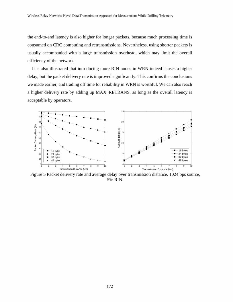
Wireless Relay Network: Novel Data Transmission Approach for Measurement-While-Drilling Telemetry
172
the end-to-end latency is also higher for longer packets, because much processing time is
consumed on CRC computing and retransmissions. Nevertheless, using shorter packets is
usually accompanied with a large transmission overhead, which may limit the overall
efficiency of the network.
It is also illustrated that introducing more RIN nodes in WRN indeed causes a higher
delay, but the packet delivery rate is improved significantly. This confirms the conclusions
we made earlier, and trading off time for reliability in WRN is worthful. We can also reach
a higher delivery rate by adding up MAX_RETRANS, as long as the overall latency is
acceptable by operators.
1 2 3 4 5 6 7 8 9 100
10
20
30
40
50
60
70
80
90
100
Transmission Distance (km)
Pac
ket D
eliv
ery
Rat
e (%
)
16 bytes24 bytes32 bytes48 bytes
1 2 3 4 5 6 7 8 9 100
5
10
15
20
25
Transmission Distance (km)
Ave
rage
Del
ay (s
)
16 bytes24 bytes32 bytes48 bytes
Figure 5 Packet delivery rate and average delay over transmission distance. 1024 bps source,
5% RIN.

Wireless Relay Network: Novel Data Transmission Approach for Measurement-While-Drilling Telemetry
173
5. Conclusion
A novel data transmission approach in MWD telemetry for oil drilling, Wireless Relay
Network (WRN), is proposed in this paper. Compared to currently used methods, WRN
excels in multiple aspects: First, it offers a competitive speed compared with MPT and
EMT. With appropriate hardware designs, an end-to-end throughput of over 660 bps over a
10 km distance is reached. Second, the wireless connection allows the whole network to
communicate continuously even during pipe installation or equipment maintenance, hence
downhole conditions can be monitored at all times. Third, WRN is completely independent
of parameters of conventional drill pipe. Since wireless nodes are easily installable, WRN
can be directly applied to the current drill pipe with almost no modifications. Last, based on
programmable microprocessors, WRN is open to further alternations on functionalities, or
even customized by operators to satisfy particular requirements. Simulation results have
shown the feasibility of WRN to establish a communication link in drill pipe. With further
experiments and realizations in the future study, WRN will prove a promising and effective
tool in the oil and gas exploration industry.
1 2 3 4 5 6 7 8 9 1020
30
40
50
60
70
80
90
100
Transmission Distance (km)
Pac
ket D
eliv
ery
Rat
e (%
)
16 bytes24 bytes32 bytes48 bytes
1 2 3 4 5 6 7 8 9 100
5
10
15
20
25
Transmission Distance (km)
Ave
rage
Del
ay (s
)
16 bytes24 bytes32 bytes48 bytes
Figure 6 Packet delivery rate and average delay over transmission distance. 1024 bps source.
10% RIN.

Wireless Relay Network: Novel Data Transmission Approach for Measurement-While-Drilling Telemetry
174
References
[1] T. R. Bates, null, and D. R. Tanguy, "Downhole measurements while drilling,"
presented at the 11th World Petroleum Congress, London. UK, 1983.
[2] J. J. Arps and J. L. Arps, “The subsurface telemetry problem – a practical solution,”
SPE Journal of Petroleum Technology, vol. 16, no. 5, pp. 487-493, May 1964.
[3] S. P. Monroe, “Applying digital data encoding techniques to mud pulse telemetry,”
presented at the Petroleum Computer Conference, Denver, Colorado, Jun. 1990.
[4] R. Hutin, R. W. Tennent, and S. V. Kashikar, “New mud pulse telemetry techniques
for deepwater applications and improved real-time data capabilities,” presented at the
SPE/IADC Drilling Conference, Amsterdam, Netherlands, 2001.
[5] C. Klotz, P. Bond, I. Wasserman, and S. Priegnitz, “A new mud pulse telemetry system
for enhanced MWD/LWD applications,” presented at the IADC/SPE Drilling
Conference, Orlando, Florida, Mar. 2008.
[6] W. R. Gardner, “High data rate MWD mud pulse telemetry,” presented at the U.S.
Department of Energy’s Natural Gas Conference, Houston, Texas, Mar. 1997.
[7] E. M. Tollefsen, A. Weber, A. B. Kramer, G. Sirkin, D. Hartman, and L. Grant,
“Logging while drilling measurements: from correlation to evaluation,” presented at
the International Oil Conference and Exhibition in Mexico, Veracruz, Mexico, Jun.
2007.
[8] N. Brown, “Electromagnetic MWD telemetry system sets depth record offshore,” Oil
and Gas Journal, vol. 100, pp. 46-47, Sept. 2002.
[9] H. Wasada, T. Sakai, R. Taniguchi, and S. Hattori, “Advanced realtime drilling control
by application of an EM-MWD system,” presented at the 14th World Petroleum
Congress, Stavanger, Norway, 1994.
[10] P. DeGauque and R. Grudzinski, “Propagation of electromagnetic waves along a
drillstring of finite conductivity,” SPE Drilling Engineering, vol. 2, pp. 127-134, Jun.
1987.

Wireless Relay Network: Novel Data Transmission Approach for Measurement-While-Drilling Telemetry
175
[11] P. K. Vong, D. Rodger, and A. Marshall, “Modeling an electromagnetic telemetry
system for signal transmission in oil fields,” IEEE Transactions on Magnetics, vol.41,
no.5, pp. 2008-2011, 2005.
[12] J. Schnitger and J. Macpherson, “Signal attenuation for electromagnetic telemetry
systems,” presented at the SPE/IADC Drilling Conference and Exhibition, Amsterdam,
Netherlands, Mar. 2009.
[13] M. J. Jellison and D. R. Hall, “Intelligent drill pipe creates the drilling network,”
presented at the SPE Asia Pacific Oil and Gas Conference and Exhibition, Jakarta,
Indonesia, Apr. 2003.
[14] M. E. Reeves, M. L. Payne, A. G. Ismayilov, and M. J. Jellison, “Intelligent drill string
field trials demonstrate technology functionality,” presented at the SPE/IADC Drilling
Conference, Amsterdam, The Netherlands, Feb. 2005.
[15] T. H. Ali, M. Sas, J. A. Hood, S. R. Lemke, A. Srinivasan, J. McKay, K. S. Fereday, C.
Mondragon, S. C. Townsend, S. T. Edwards, M. Hernandez, and M. Reeves, “High
speed telemetry drill pipe network optimizes drilling dynamics and wellbore
placement,” presented at the IADC/SPE Drilling Conference, Orlando, Florida, Mar.
2008.
[16] S. Allen, C. McCartney, M. Hernandez, M. E. Reeves, A. Baksh, and D. MacFarlane,
“Step-change improvements with wired-pipe telemetry,” presented at the SPE/IADC
Drilling Conference and Exhibition, Amsterdam, The Netherlands, Mar. 2009.
[17] D. Veeningen, “Novel high speed telemetry system with measurements along the
string mitigate drilling risk and improve drilling efficiency,” presented at the Brasil
Offshore Conference and Exhibition, Macae, Brazil, Jun. 2011.
[18] H. Naseri and C. Liu, “Electromagnetic telemetry in measurement-while-drilling with
small RF-transceivers,” presented at the CPS/SEG Beijing 2009 Conference and
Exposition, Beijing China, Apr. 2009.
[19] 2.4-GHz Bluetooth Low Energy System-on-Chip, Texas Instruments Inc., Dallas, TX,
2010.

Wireless Relay Network: Novel Data Transmission Approach for Measurement-While-Drilling Telemetry
176
[20] I. Jawhar, N. Mohamed, M. M. Mohamed, and J. Aziz, "A routing protocol and
addressing scheme for oil, gas, and water pipeline monitoring using wireless sensor
networks," in Wireless and Optical Communications Networks, 2008. WOCN '08. 5th
IFIP International Conference on, 2008, pp. 1-5.
[21] M. A. Garcia, R. S. G. Villar, A. L. R. Cardoso, and J. C. T. B. Moraes, "A low-cost
and high-reliability communication protocol for remote monitoring devices,"
Instrumentation and Measurement, IEEE Transactions on, vol. 53, pp. 612-618, 2004.

Wireless MWD Telemetry System Using MEMS Radio
177
CHAPTER 7
Wireless MWD Telemetry System Using MEMS Radio
Abstract The measurement-while-drilling (MWD) logging tool measures the geophysical
properties of the formation that are critical in understanding the downhole environment.
Current MWD telemetry techniques suffer from low data rate transmission. Improvement
of MWD logging technology is required by oil and gas industry.
The purpose of this study is to design a high speed electromagnetic telemetry relay
network that utilizes small RF wireless transceivers. These RF transceivers will be placed
inside the drilling pipe. The MWD data collected at the bottom of the drilling pipe can be
transmitted to the processor at the surface by using a large number of these RF
transceivers. This method of transmission can achieve high data rate of up to a few kilo
bits per second which significantly surpasses the conventional telemetry techniques.
In this paper we use MEMS radio to build the wireless network. The MEMS radio has
advantages of high sensitivity and low power consumption which are ideal for the system.
It also has excellent receiver selectivity and blocking performance so that it will be
reliable for the wireless network.
The transceivers built for this project were tested, the results show that the wireless
telemetry system can achieve high speed data rate and low packet error rate. The results
have proved the application of the transceiver in MWD telemetry.
1 Introduction
Nowadays, electrical logging is recognized as the only measurement to distinguish
hydrocarbon from water. Lots of modern oil and gas wells are drilled directionally.
Modern techniques now transmit continuous information from the bottom to the surface.
This is known as measurement-while-drilling (MWD) or logging while drilling (LWD).

Wireless MWD Telemetry System Using MEMS Radio
178
There are different methods of data transmission in MWD logs. Among these, Mud Pulse
Telemetry (MDT) is the most common method used by MWD tools. Pulses generated
downhole travel through drilling pipe within the drilling fluid towards the surface where
they are received from pressure sensors. The received signals are processed by computers
on surface and useful information will be reconstructed from them. Many factors restrict
the speed of data transmission. Better methods of data transmission are still being
developing by oilfield service companies. Electromagnetic telemetry (EMT) is an
alternative to MPT. It has been studied for years. Many EMT tools have been designed
by different companies on the market now. However, these tools still have limitations
under specific applications, and have not yet gained universal acceptance by the oilfield
service industry.
This report focuses on a novel electromagnetic telemetry wireless network which
utilizes a large number of small size microwave transceivers to transmit data. By
transmitting information to one another, these transceivers create a wireless network
inside the drilling pipe from the bottom of the borehole tool to the surface. The schematic
of the EMT wireless network is shown in Fig. 1.
Fig. 1 Schematic of the EMT wireless network.
The downhole tool is one end of this wireless network while the surface receiver is the
other end. The data transmission can be full duplex or half duplex depending on the
requirements. So not only can we transmit data from downhole tool to surface, but also it
creates a communication link from surface to downhole tool. Thus the drilling tool at the
bottom of the pipe can be more precisely controlled. This electromagnetic telemetry
wireless network leads the drilling procedure to be more efficient due to real-time data
transmission.

Wireless MWD Telemetry System Using MEMS Radio
179
The Texas Instrument CC2510 and CC2511 low-power system-on-chip 2.4 GHz RF
transceiver used in this project can achieve data rates of up to 500 Kbps, which is much
higher than conventional telemetry technique. The entire system includes the antenna and
the circuit parts. A loop antenna is used for this system. The printed circuit board (PCB)
is placed inside the loop antenna. The RF wireless transceiver and other external
components are soldered on the PCB.
2 Antenna System Design
The downhole environment is so complicated which makes the radiation efficiency of
the transceiver very challenging. The antenna system is critical in this project because
efficient radiation of the RF transceiver largely depends on the antenna. The important
factors, that need to be considered when we designing the antenna, include features of the
drilling pipe, cutoff frequency of the pipe and resonant frequency of the RF transceiver.
A borehole model has the following parameters.
1. Drilling pipe diameter = 4 inches
2. Borehole diameter = 8 inches
The electromagnetic signal attenuates when propagating along the drilling pipe. The
drilling fluid inside the pipe largely causes the attenuation of the EM signal. The complex
permittivity of the mud is given by
ωσεε j
d−=
∧
, (1)
where
εεε rd 0= , (2)
and rε , σ , 0ε are mud relative permittivity, mud conductivity and permittivity of the
free space, respectively. The complex epsilon of the mud is used in calculating its
attenuation constant or dα . The relationship between wave number ( k ), critical wave
number ( ck ) and the propagation constant ( zk ) is given by
22zc kkk −= , (3)

Wireless MWD Telemetry System Using MEMS Radio
180
where
αβ jk z −= . (4)
The real part (β ) is the phase constant and imaginary part (α ) is the attenuation constant,
respectively. Combining the last two equations we have 222)( ckkj −=− αβ , (5)
or
02222 2 μεωμεωαβαβ ccj −=−− , (6)
and finally
02
0222 )2()()2(2 μεπ
ωσεεμπαβαβ cr fjfj −−=−− . (7)
In this equation, cf is the cutoff frequency and μ is the free space permeability,
respectively. The cutoff frequency is a function of the geometry of the waveguide and is
equal to[2]
μεπμεπ apk
f nmccTEnm 2
'2
== , (8)
where nmp ' is the thn positive root of 0)(' =xJ m , and 'mJ is a Bessel function of the first
kind of order m [3]. The values of the first few such roots are listed in Table 1.
Table 1 Values of nmp' for TE modes of a circular waveguide
N 1'np 2'np 3'np
0 3.832 7.016 10.174
1 1.841 5.331 8.536
2 3.054 6.706 9.970
The finite conductivity of the steel pipe is another reason of the attenuation when the
EM signal propagating inside the drilling pipe. The drilling pipe is treated as a cylindrical

Wireless MWD Telemetry System Using MEMS Radio
181
waveguide. We assume the drilling pipe is in a cylindrical shape all the way from the top
of the surface to the bottom of the well. Fig. 2[2] shows the field lines for some of the
lower order modes of a circular waveguide.
Fig. 2 Field lines for some of the lower order modes of a circular waveguide.
We choose TE11 mode for the wireless network in this project because TE11 mode has
the lowest cutoff frequency. Given that the diameter of a drilling pipe is 4 inches and the
conductivity is 6104.1 × S/m, the cutoff frequency for the TE11 mode of this cylindrical
waveguide is 1.7 GHz. In order to match field lines of TE11 mode, different types of
antenna have been designed and simulated for optimal selection.
2.1. Dipole Antenna
A dipole antenna can be made of a simple wire with a center-fed driven element. It
consists of two metal conductors of rod or wire. The two metal conductors are oriented
parallel and collinear with each other, with a small space between them. The dipole
antenna is the simplest practical antennas from a theoretical point of view. A typical
dipole antenna is made by two quarter wavelength ( 4/λ ) conductors or elements placed
back to back. The radio frequency voltage is applied to the antenna at the center, between
the two conductors. A standing wave on an element of a quarter wavelength yields the
greatest voltage differential. The larger the differential voltage is, the greater the current
between the elements will be.

Wireless MWD Telemetry System Using MEMS Radio
182
Assuming a sinusoidal distribution, the current impressed by this voltage differential
is given by:
0 cosi tI I e klω= , (9)
where ω is the angular frequency, 2k πλ
= is the wavenumber, and l is the length of the
conductor, respectively.
The electric field of a radiating electromagnetic wave is given by:
( )0
0
cos( cos )2
2 sini t kriIE e
crω
θ
π θ
πε θ−−
= , (10)
where Eθ is the far electric field of the electromagnetic wave radiated in the θ direction,
0ε is the permittivity of vacuum, c is the speed of light in vacuum, r is the distance
from the point on the conductor to where the electrical field Eθ is evaluated, respectively.
A dipole antenna model is built in CST Microwave Studio as shown in Fig. 3.
Fig. 3 The dipole antenna model in CST Microwave Studio
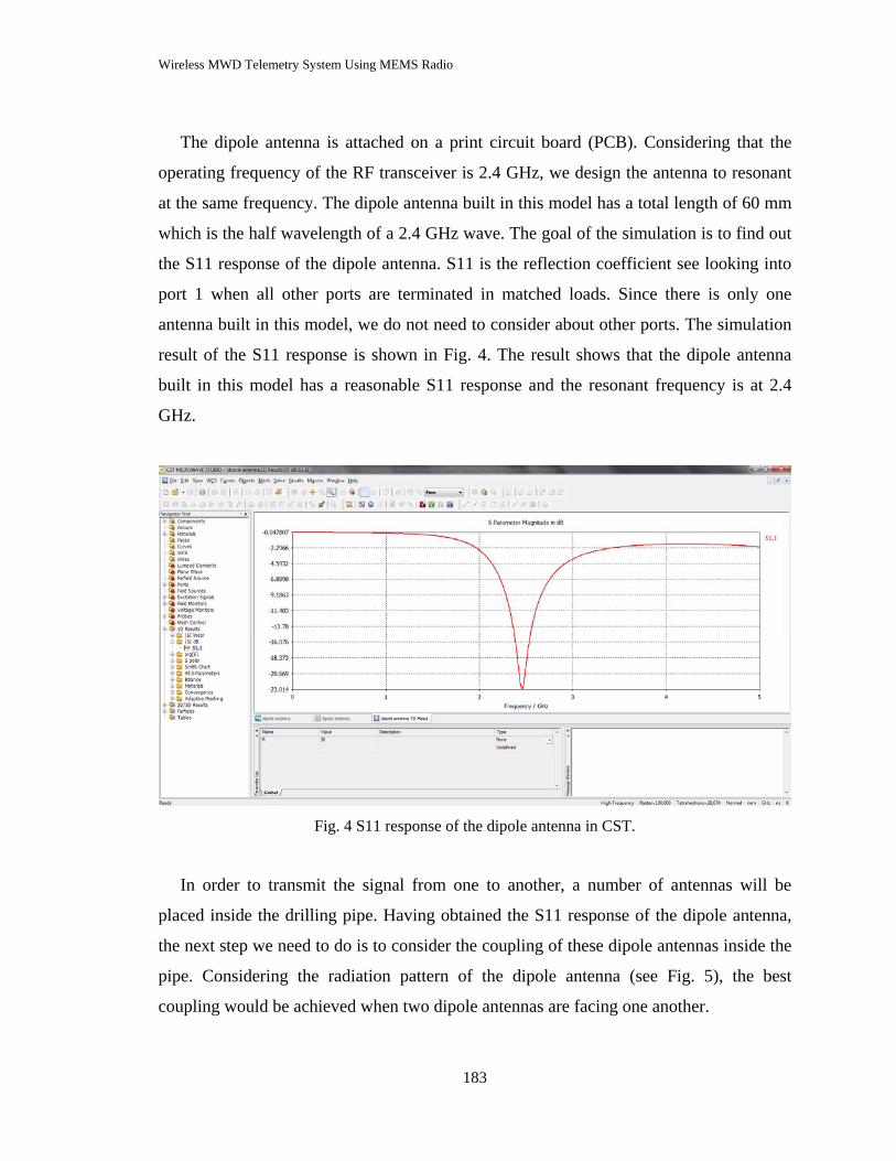
Wireless MWD Telemetry System Using MEMS Radio
183
The dipole antenna is attached on a print circuit board (PCB). Considering that the
operating frequency of the RF transceiver is 2.4 GHz, we design the antenna to resonant
at the same frequency. The dipole antenna built in this model has a total length of 60 mm
which is the half wavelength of a 2.4 GHz wave. The goal of the simulation is to find out
the S11 response of the dipole antenna. S11 is the reflection coefficient see looking into
port 1 when all other ports are terminated in matched loads. Since there is only one
antenna built in this model, we do not need to consider about other ports. The simulation
result of the S11 response is shown in Fig. 4. The result shows that the dipole antenna
built in this model has a reasonable S11 response and the resonant frequency is at 2.4
GHz.
Fig. 4 S11 response of the dipole antenna in CST.
In order to transmit the signal from one to another, a number of antennas will be
placed inside the drilling pipe. Having obtained the S11 response of the dipole antenna,
the next step we need to do is to consider the coupling of these dipole antennas inside the
pipe. Considering the radiation pattern of the dipole antenna (see Fig. 5), the best
coupling would be achieved when two dipole antennas are facing one another.
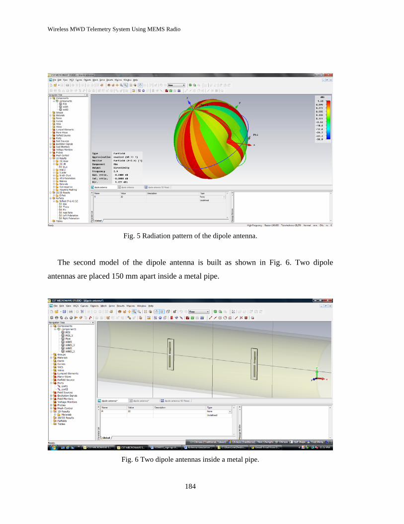
Wireless MWD Telemetry System Using MEMS Radio
184
Fig. 5 Radiation pattern of the dipole antenna.
The second model of the dipole antenna is built as shown in Fig. 6. Two dipole
antennas are placed 150 mm apart inside a metal pipe.
Fig. 6 Two dipole antennas inside a metal pipe.

Wireless MWD Telemetry System Using MEMS Radio
185
The coupling of the two dipole antennas is determined by the S21 response. S21 is the
transmission coefficient from port 1 to port 2. A reasonable S21 response would mean an
effective radiation performance of the antennas. The S11 and S21 response of the second
model are shown in Fig. 7 and Fig. 8.
Fig. 7 S11 response of two dipole antennas.

Wireless MWD Telemetry System Using MEMS Radio
186
Fig. 8 S21 response of two dipole antennas.
As shown in the figures, the S11 and S21 response of the two dipole antennas are
reasonable. The results have shown the efficiency of the dipole antenna. The only
problem is the size of the dipole antenna. Considering that the diameter of the drilling
pipe is about 4-inch, a dipole antenna with a length of 60 mm would be too large for our
application. Placing a dipole antenna inside the pipe would probably block the drilling
fluid. Therefore the dipole antenna becomes not practical for this project. Another type of
antenna, that has efficient radiation performance but smaller size, is needed. The loop
antenna becomes our next consideration.
2.2. Loop Antenna
A loop antenna is consisting of a loop of wire, or other electrical conductor with its
ends connected to a balanced transmission line. The loop antenna is simple, inexpensive,
and very versatile. It can take many different forms such as a square, rectangle, triangle,
circle and many other configurations. The loop antenna is the most popular type because
of its simplicity in construction and analysis. Most of the applications of loop antennas
are in the HF (high frequency, 3-30 MHz), VHF (very high frequency, 30-300 MHz), and

Wireless MWD Telemetry System Using MEMS Radio
187
UHF (ultra high frequency, 300-3,000 MHz) bands. The field pattern of the loop antenna
is similar to that of a magnetic dipole antenna with a null perpendicular to the plane of
the loop and with its maximum along the plane of the loop. As the overall length of the
loop increases and its circumference approaches one free-space wavelength, the
maximum of the pattern shifts from the plane of the loop to the axis of the loop which is
perpendicular to its plane.
The circumference of an electrically large loop antenna is about a free-space
wavelength ( ~C λ ). The geometry for far-field analysis of a loop antenna is shown in
Fig. 9.
Fig. 9 Geometry for far-field analysis of a loop antenna.

Wireless MWD Telemetry System Using MEMS Radio
188
The distance R can be approximated by:
2 2 22 sin cos ' 2 sin cos 'R r a ar r arθ φ θ φ= + − − (11)
for r a .
R can be reduced to:
021 sin cos ' sin cos ' cosaR r r a r ar
θ φ θ φ ψ− = − = − , (12)
The electric potential at a certain point is given by:
2 sin cos '00
cos ' '4
jkrjkaa I eA e d
rπ θ φ
φμ φ φπ
−+∫ (13)
It can be separated into two terms as:
2sin cos ' sin cos '00
[ cos ' ' cos ' ']4
jkrjka jkaa I eA e d e d
rπ πθ φ θ φ
φ π
μ φ φ φ φπ
−+ ++∫ ∫ (14)
The second term within the brackets can be rewritten by making a change of variable of
the form
' ''φ φ π= + (15)
Therefore the equation (14) can be written as
sin cos ' sin cos ''00 0
[ cos ' ' cos '' '']4
jkrjka jkaa I eA e d e d
rπ πθ φ θ φ
φμ φ φ φ φπ
−+ −−∫ ∫ (16)
Each of the integrals in (16) can be integrated by the formula
cos
0( ) cos( )n jz
nj J z n e dπ φπ φ φ+= ∫ (17)
where ( )nJ z is the Bessel function of the first kind of order n .
Thus Aφ can be reduced to
01 1[ ( sin ) ( sin )]
4
jkra I eA jJ ka jJ karφ
μ π θ π θπ
−
− − (18)
The Bessel function of the first kind and order n is defined by the infinite series 2
0
( 1) ( / 2)( )!( )!
m n m
nm
zJ zm m n
+∞
=
−=
+∑ (19)
( ) ( 1) ( )nn nJ z J z− = − (20)

Wireless MWD Telemetry System Using MEMS Radio
189
When n=1
1 1( ) ( )J z J z− = − (21)
Thus the electric potential Aφ is given by
01( sin )
2
jkra I eA J karφ
μ θ−
(22)
The next step is to find out the electric field and magnetic field associated with the
electric potential Aφ . According to Maxwell’s equations and equation (22), the E- and H-
fields are given by
0rE Eθ = (23)
01( sin )
2
jkrak I eE J karφ
η θ−
(24)
0rH Hφ = (25)
01( sin )
2
jkrE akI eH J kar
φθ θ
η
−
− = − (26)
where 377Ohmsη = is the wave impedance in free-space. [1]
The model of a loop antenna built for our project is shown in Figure 2.9. The
excitation signal is added at the bottom part of the loop antenna. The loop antenna needs
to resonant at 2.4 GHz of which the wavelength is about 125 mm. According to the
characteristic of the electrically large loop antenna, the circumference is about a free-
space wavelength ( ~C λ ). Thus, the radius of the loop antenna built in Fig. 10 is 20 mm,
giving the loop antenna a relatively small size.
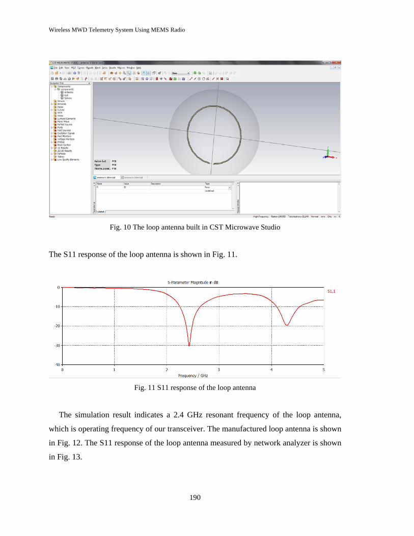
Wireless MWD Telemetry System Using MEMS Radio
190
Fig. 10 The loop antenna built in CST Microwave Studio
The S11 response of the loop antenna is shown in Fig. 11.
Fig. 11 S11 response of the loop antenna
The simulation result indicates a 2.4 GHz resonant frequency of the loop antenna,
which is operating frequency of our transceiver. The manufactured loop antenna is shown
in Fig. 12. The S11 response of the loop antenna measured by network analyzer is shown
in Fig. 13.

Wireless MWD Telemetry System Using MEMS Radio
191
Fig. 12 Manufactured loop antenna.
Fig. 13 Measure S11 response of the loop antenna on network analyzer
Based on the simulation results and lab measurements, a loop antenna has excellent
radiation performance and small size. Thus, the loop antenna is chosen for our system.

Wireless MWD Telemetry System Using MEMS Radio
192
3 Antenna System Design
The TI CC2510/CC2511 RF transceivers are chosen for this project. It operates at 2.4
GHz in a voltage range from 2.0V to 3.6V. The advantage of CC2510/CC2511 RF
transceivers are the embedded microcontroller and the low current and power
consumption. The receiving current consumption is 17.1 mA at 2.4 kbps and the
transmitting current consumption is 16 mA at -6 dBm output power. The lowest power
consumption at operating mode is 0.3 Aμ in PM3. Compare to other RF transceivers,
CC2510/CC2511 have a high sensitivity of -103 dBm at 2.4 kbps and their maximum
data rate is up to 500 kbps. The block diagram of the CC2510/CC2511 RF transceiver is
shown in Fig. 14.
Fig. 15 shows the top view of CC2511 pin-out. This chip has 17 general purpose
input-output pins used for programming, debugging and testing. These pins are controlled
by ports P0 (P0_0 to P0_5), P1 (P1_0 to P1_7) and P2 (P2_0, P2_1, P2_2). The 8051
microcontroller, the ADC and the RF front end of this chip run on two crystal oscillators.
The 48.0 MHz crystal oscillator is connected to Pin 20 and Pin 21. And the 32.768 KHz
crystal oscillator is connected to Pin 17 and Pin 18. For the CC2510 transceiver, a 26.0
MHz crystal oscillator is used instead of the 48.0 MHz crystal oscillator.
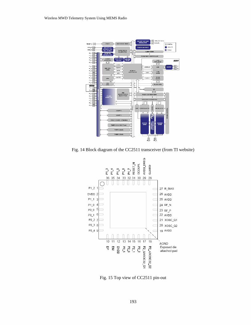
Wireless MWD Telemetry System Using MEMS Radio
193
Fig. 14 Block diagram of the CC2511 transceiver (from TI website)
Fig. 15 Top view of CC2511 pin-out
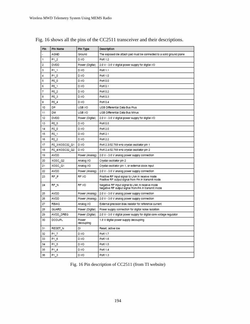
Wireless MWD Telemetry System Using MEMS Radio
194
Fig. 16 shows all the pins of the CC2511 transceiver and their descriptions.
Fig. 16 Pin description of CC2511 (from TI website)

Wireless MWD Telemetry System Using MEMS Radio
195
The schematic of the RF transceiver application circuit is shown in Fig. 17. Only a
few external components are required for using the CC2510/CC2511 transceivers. The
power supply has been properly decoupled using decoupling capacitors. Fig. 18 shows
the layout of the board in OrCAD.
Fig. 17 Schematic of the application circuit designed in OrCAD Capture
Fig. 18 The layout of the application circuit designed in OrCAD
The CC2510/CC2511 transceivers are powered up via the VDD pin and the power
supply range is 2.0 V to 3.6V. The power will be supplied by 3V cell batteries. The

Wireless MWD Telemetry System Using MEMS Radio
196
MCP1256 charge pump is included in the circuit to ensure the performance of the chip.
The charge pump will generates a constant 3.3V output voltage to the CC2510/CC2511
transceivers from a 1.8V to 3.6V input. The schematic of the charge pump and its
connection with the transceiver is shown in Fig. 19. Fig. 20 shows the manufactured
board. The size of the board can be compared to a quarter coin in the figure.
Fig. 19 Schematic of the charge pump.

Wireless MWD Telemetry System Using MEMS Radio
197
Fig. 20 The manufactured board based on the OrCAD layout.
Smart Flash Programmer provided by Texas Instrument is used for the programming
of the RF transceiver. Fig. 21 shows the interface of the Smart Flash Programmer.
Fig. 21 Interface of Smart Flash Programmer.

Wireless MWD Telemetry System Using MEMS Radio
198
The CC2510 evaluation kit, including the SmartRF04 evaluation board shown in Fig.
22, provided us with other hardware and software that are needed for programming the
RF transceiver. The board is connected to computer through a CC Debugger for
programming as shown in Fig. 23.
Fig. 22 SmartRF04 Evaluation Board.
Fig. 23 Programming the transceiver with CC Debugger.

Wireless MWD Telemetry System Using MEMS Radio
199
4 Lab test and experimental results
4.1 Signal propagation inside a pipe
The first thing we want to make sure is that the signal can propagate inside a drilling
pipe. As mentioned in the previous chapter, the pipe is treated as a lossy circular
waveguide. The first experiment is to simulate a real MWD environment with a used
drilling pipe. The schematic of this experiment is shown in Fig. 24.
Fig. 24 Schematic of the signal propagation experiment.
A 5 feet long metal pipe is used in this experiment. The transceiver with the loop
antenna is connected to the computer. It is placed at one end of the pipe. The spectrum
analyzer (Hewlett-Packard E7403A) is put at the other end of the pipe to detect the
received signal (see Fig. 25).

Wireless MWD Telemetry System Using MEMS Radio
200
Fig. 25 Probing the electromagnetic wave inside a pipe.
The transceiver generates an electromagnetic (EM) wave. The input power of this EM
wave is 1 mW. The received signal detected by the spectrum analyzer is shown in Fig. 26.

Wireless MWD Telemetry System Using MEMS Radio
201
Fig. 26 Signal received by the spectrum analyzer.
The reference of the measurement is 107 dB Vμ which equals to 1 mW. As shown in
the figure, the received signal has a value of 82.02 dB Vμ at 2.4 GHz, which is 0.0032
mW. The power attenuation of the received signal compared to the input signal is -24.95
dB .
The experiment results prove that the electromagnetic (EM) wave will propagate
inside the drilling pipe when the frequency of the EM wave is greater than the cutoff
frequency of the four inch pipe.
4.2 Packet error rate (PER) test in open air
The packet error rate (PER) test of data transmission between two transceivers has
been performed. The first experiment with different data rates is tested in open air.

Wireless MWD Telemetry System Using MEMS Radio
202
Table 2 Packet error rate at 2.4 kbps
Distance [m] PER @2.4 kbps
1 0%
2 0%
3 0%
4 0%
5 0%
6 0%
7 0%
8 0%
Table 3 Packet error rate at 56 kbps
Distance [m] PER @56 kbps
1 0%
2 0%
3 0%
4 0%
5 0%
6 0%
7 0%
8 0%

Wireless MWD Telemetry System Using MEMS Radio
203
Table 4 Packet error rate at 180 kbps
Distance [m] PER @180 kbps
1 0%
2 0%
3 0%
4 0%
5 0%
6 0%
7 2%
8 6%
Table 5 Packet error rate at 210 kbps
Distance [m] PER @56 kbps
1 0%
2 1%
3 2%
4 5%
5 18%
6 37%
7 61%
8 92%
4.3 Packet error rate (PER) test inside a 5-inch pipe
The second experiment is to test the packet error rate inside a pipe. The pipe is shown
in the previous picture. The length of the pipe is 5 inches. Different data rates are set. The
result is shown in Table 6.

Wireless MWD Telemetry System Using MEMS Radio
204
Table 6 Packet error rate inside a 5-inch pipe
Data rate [kbps] Packet error rate
2.4 0%
56 0%
70 4%
90 10%
120 19%
150 41%
180 72%
210 100%
4.4 Three nodes relay network test
Three boards are used for the relay network test. These three nodes are transmitter,
repeater and receiver. The boards are connected to the computer through RS232 serial
adapters so that the information can be seen in hyper-terminal windows. The three
devices used in this experiment are shown in Fig. 27.
Fig. 27 Three nodes.
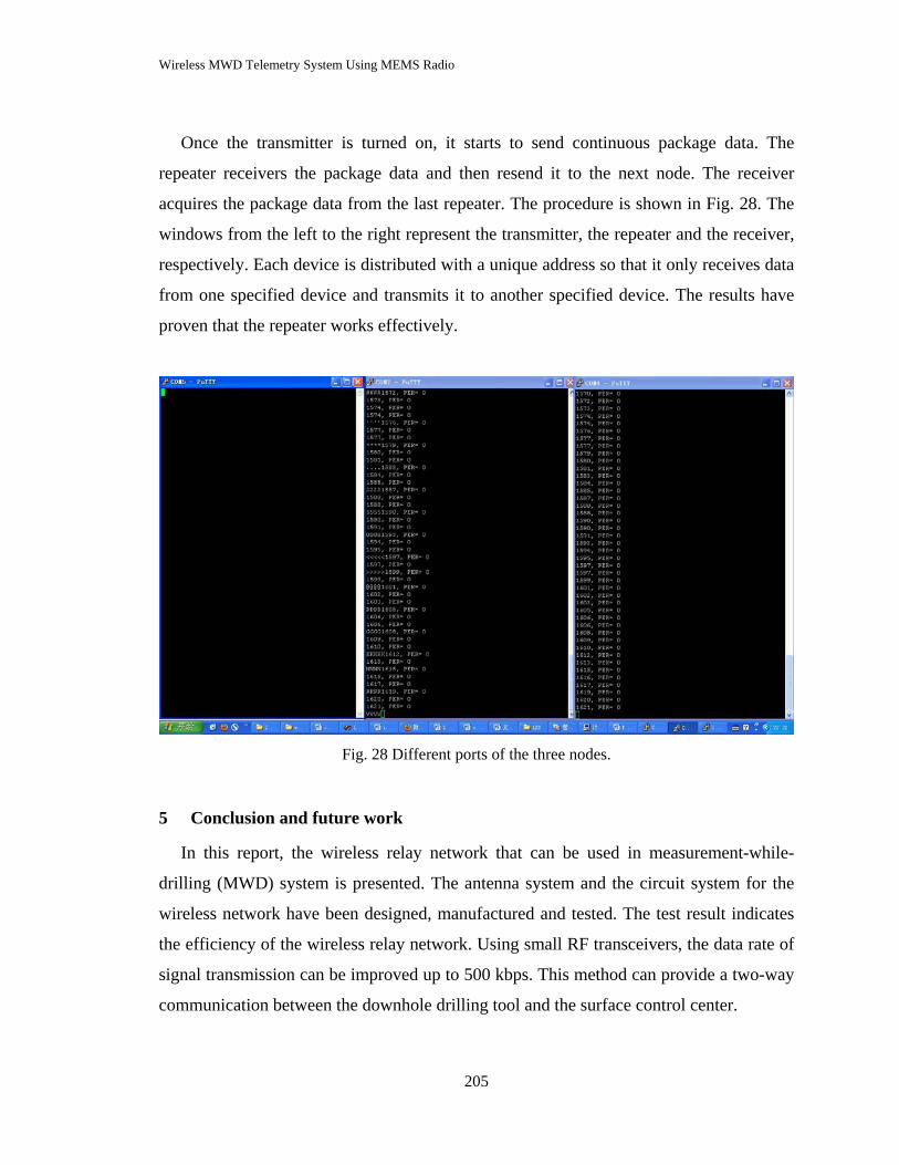
Wireless MWD Telemetry System Using MEMS Radio
205
Once the transmitter is turned on, it starts to send continuous package data. The
repeater receivers the package data and then resend it to the next node. The receiver
acquires the package data from the last repeater. The procedure is shown in Fig. 28. The
windows from the left to the right represent the transmitter, the repeater and the receiver,
respectively. Each device is distributed with a unique address so that it only receives data
from one specified device and transmits it to another specified device. The results have
proven that the repeater works effectively.
Fig. 28 Different ports of the three nodes.
5 Conclusion and future work
In this report, the wireless relay network that can be used in measurement-while-
drilling (MWD) system is presented. The antenna system and the circuit system for the
wireless network have been designed, manufactured and tested. The test result indicates
the efficiency of the wireless relay network. Using small RF transceivers, the data rate of
signal transmission can be improved up to 500 kbps. This method can provide a two-way
communication between the downhole drilling tool and the surface control center.

Wireless MWD Telemetry System Using MEMS Radio
206
For the whole wireless relay network, more models will be made to provide more
nodes between two ends so that the packet error rate can be reduced and the transmission
will be more accurate. The RF performance improvement of the repeater and the
optimization of the wireless relay network are currently being studied.
Wireless MWD Telemetry System Using MEMS Radio
207
References
[1] Constantine A. Balanis, “Antenna Theory Analysis and Design,” pp. 231-246, 2005.
[2] David M. Pozar, “Microwave Engineering”, pp. 117-126, 2005
[3] Hamid Naseri, “Electromagnetic Telemetry in Measurement While Drilling with a
Wireless Relay Network”, PHD Dissertation, Department of Electrical and Computer
Engineering, University of Houston, Houston, TX, May 2009.
[4] A. C. Balanis, “Advanced Engineering Electromagnetics,” pp. 728-731, 1989
[5] Texas Instruments, data sheet of Low-Power SoC ( System-on-chip) with MCU,
memory, 2.4 GHz RF Transceiver, and USB
[6] Texas Instruments, CC1111/CC2511 USB HW User’s Guide.PDF
[7] Digikey, data sheet of MCP1256 Charge Pump
[8] J. P. Carcione, “A Telegraph equation for electric-telemetering in drill string,” IEEE
Transaction on Geosciences and Remote Sensing, vol. 40, pp. 1047-1053, 2002
[9] L. C. Shen, “The Transmission-Line Model of an Insulated Antenna with a Two-
Layer Eccentric Insulator,” IEEE Transaction on Antennas and Propagation, vol. 24,
pp. 895-896, Nov 1976
[10] D. V. Ellis, “Well Logging for Earth Scientists,” Elsevier Science Publishing Co.,
Inc., p 145, 1978
[11] N. Brown, “Electromagnetic MWD telemetry system sets depth record offshore,”
Oil and Gas Journal, vol. 100, pp. 46-47, Sep 2002

208
APPENDIX A List of Theses and Dissertations
The following are senior theses, master theses, and doctoral dissertations completed by
the research staff of the Well Logging Laboratory.
1982 Shabbir A. Chowdhury
Investigation of Electrode Effects in the Measurement of Impedance of Water Saturated Rocks at Low Frequencies (M. S. Thesis) Shey-Min Su Measurements of Dielectric Constant and Conductivity of Petroleum Reservoir Rocks at Microwave Frequencies (M. S. Thesis)
1984 Hardy X. J. Guo
Physical Modelling of Induction Logging in Dipping Beds (M. S. Thesis) S. C. Frank Huang Techniques for Measuring the Dielectric Properties of Samples Using Coaxial-Line and Insulated Antenna (Ph. D. Dissertation) Shahryar Darayan High-Temperature Electromagnetic Properties of Reservoir Rocks at UHF (M. S. Thesis)
1985 Herzl Marouni Dielectric Constant and Conductivity Measurement of Reservoir Rocks in the Range of 20-50 MHz (M. S. Thesis) Gong Li Physical Modelling of Induction Logging in Dipping Beds with a Large Borehole (M. S. Thesis)
1986 Michel S. Bittar
Laterolog Scale Modelling Experiments (M. S. Thesis)

209
Nancy S. Pollard Computer Simulation of Induction Tool Resistivity Readings in Multiple Layer Formations (Senior Thesis) Kobina O. Eshun A New Design for the WLL Induction Logging Model Facility (Senior Thesis)
1987 Lee-Hwa Lue Wang
Inversion of Induction Logging Data in Horizontally Layered Formation (M. S. Thesis) Ming Huang Modeling Medium Inhomogeneity in Induction Logging (M. S. Thesis) Xin Lin Microwave Dipmeter (M. S. Thesis)
1988 Kuang-Fu Han Dielectric Constant Measurement of Saline Solution at 1.1 GHz (M. S. Thesis) Muhammad N. A. Ansari Effect of Dissimilar Scale Factors for Length and Diameter on Shallow Laterolog Scale-Model Tool Response (M. S. Thesis) Kobina O. Eshun A Laboratory Model of the Focused Induction Logging Sonde (M. S. Thesis) Chi-Ming Lam Modelling the Electrode Well-Logging Sonde by the Method of Finite Elements (M. S. Thesis) Chia-Hsiang Lin Conductivity Measurement at Low Frequencies Using a Digital Bridge (M. S. Thesis)
210
1990 Yongdong He
Input Impedance of an Antenna and Its Application in Complex Permittivity Measurement at High Frequencies (Ph. D. Dissertation) Michael S. Bittar Study of Resistivity Sondes by Scale Modeling and Three-Dimensional Finite Element Method (Ph. D. Dissertation)
1991 Xiaolu Zhao
Numerical Analysis of a TM010 Cavity for Dielectric Measurement (M. S. Thesis)
1992 Chun-ta Chao
Wellog Simulator: Simulation for Induction Tool in Layered Medium (M. S. Thesis) Yu-zhi Li Monopole Antenna as a Probe for Measuring Dielectric Properties at 300-1100 MHz (M. S. Thesis) Tien-min Wang Electrical Properties of Saline Solution and Contaminated Soils (M. S. Thesis)
1993 Shahryar Darayan
Measurement of Dielectric Permittivity and Conductivity of Samples Using Guarded Electrodes (Ph. D. Dissertation) Ming Huang Resistivity Measurement in Laboratory and Field Environments (Ph. D. Dissertation) Yongchun Zhang Induction Log Inversion and Cross-Hole Electromagnetic Tomography (Ph. D. Dissertation)
1994 Jiazhi Chui
Simulation of Measurement-While-Drilling Tool in Cylindrical Media (M. S. Thesis)

211
Liang (Linda) Lin Simulation of Induction Tools in Dipping Beds (M. S. Thesis) Yongmin Zhang A Time-Domain Modeling and Inversion Technique and Its Applications to Electromagnetic Subsurface Sensing (Ph. D. Dissertation)
1995 Qian Gu
Evaluation of Approximations Used to Simulate MWD Tools in Layered Formations (M. S. Thesis) Xuhua Hu Radial Resistivity Profile Invasion Using Array Induction Logs (M. S. Thesis) Xiaoning Zhang Quick Look Inversion of Through Casing Resistivity Measurement (M. S. Thesis)
1996 Rohit Gaikwad
Scale Modeling of the Through-Casing Resistivity Tool (M.S. Thesis) Feng Gao A Scale Model of the Through-Casing Resistivity Measurement (M.S. Thesis) Jing Lin Three Dimensional Finite-Element Mesh Generation and Interactive Computer Graphic Visualization System (M. S. Thesis) Xiao-bing Wu Inversion of Induction Logs in Dipping Beds (Ph.D. Dissertation)
Ruilin Zhong Simulation the Effects of Casing Corrosion on the Through-Casing Resistivity Logs (M. S. Thesis)

212
Jiang Zhu Modeling and Evaluation of MWD Resistivity Tool in Horizontal Well (M. S. Thesis)
1997 Ji Fang
Algorithms for Inversion of Induction Logs in Dipping Bed (M. S. Thesis)
Xiang Tian Numerical Simulations of Induction and MWD Logging Tools and Data Inversion Method with X-Window Interface on a UNIX Workstation (Ph.D. Dissertation) Yuanzheng Ming Simulation of Through-Casing Resistivity Logging (M. S. Thesis) Hongxu Wu Theoretical Studey of the Effective Dielectric Constant of 3D Mixtures with Applications in Soil Water Content Measurement (M.S. Thesis)
1998 Jingjing Sun
Simulation of Induction Logging in 2D Formation using the Born Approximation (M. S. Thesis) Shu Huang Computer Simulation of Microwave Flow Meter (M. S. Thesis) Long Wang 3-D Numerical Modeling of Induction Resistivity Tool for Well Logging Using Finite Element Method (Ph.D. Dissertation)
1999 Huage Zheng Physical Modeling of an Automated Through-Casing Resistivity Measurement System (M. S. Thesis)
213
Hanming Wang Finite Element Analysis of Resistivity Logging (Ph.D. Dissertation)
2000 Yuan Hu
Simulation of Induction and MWD Logging in Wells with Varying Dip Angles (M. S. Thesis) Jian Li 2-D Inversion for Induction and MWD Logs (Ph.D. Dissertation)
Ji Li Modeling Electrode-type Logging Tools in 2-D Formations by Finite Element Method (M. S. Thesis) Guoyu Hu Two-dimensional Cross-well Forward Modeling and Inversion (M. S. Thesis)
2001 Chatrpol Lertsirimit
Apparatus for Measuring Conductivity Tensor of Anisotropic Samples in the Laboratory (M. S. Thesis) Chuanxiao Li A Graphical Interface for Well-Logging Codes (M. S. Thesis)
2002 Pei Jin
Laboratory Technique for Measuring Conductivity Tensor of Anisotropic Samples (M. S. Thesis) Lili Zhong Simulation of Multi-Component Induction Tool in Dipping Beds (M. S. Thesis) Wei Gao 3D Transmission Line Matrix Method and Application Interface (M. S. Thesis)
2004 Lili Zhong
214
Simulation of Tri-Axial Induction Tools in Dipping Anisotropic Beds (Ph.D. Dissertation) Shanjun Li Analysis of Complex Formations Using Computer Techniques (Ph.D. Dissertation) Weishan Han 3D Finite Element Simulation Method of Induction and MWD Tools (Ph.D. Dissertation)
2005 Jing Li
Electrical Property Measurement of Rocks in the Range of 10kHz –1.1GHz (M.S. Thesis)
2006 Xueshen Yu Inversion of Tri-Axial Induction Logs in Anisotropic Formation (M.S. Thesis)
2007 David Navarro Effects of Invasion Transient on Resistivity Time-Lapsed Logging (M.S. Thesis)
2008 Asutosh Bhardwaj 1-D Inversion of Tri-axial Induction Logs in Anisotropic Medium (M.S. Thesis)
Yumei Tang Modeling and Inversion of Multicomponent Induction Logs in Biaxial Anisotropic Formation (Ph.D. Dissertation)
2009 Li Zhong
Response of Induction and LWD Tools in Multiple Cylindrically Layered Media (M.S. Thesis) Jinjuan Zhou Application of Finite Element Method in Solving Well Logging Problems (Ph.D. Dissertation)

215
Hamid Naseri Electromagnetic Telemetry in Measurement-While-Drilling with a Wireless Relay Network (Ph.D. Dissertation) Mark Collins Response of MWD Resistivity Tools in Eccentric Cylindrically Layered Media (M.S. Thesis)
2010 Chen Guo Research on Ultra Wideband(UWB) Antenna and Radar Application (Ph.D. Thesis) Huaping Wang
Ground Penetrating Radar with Wireless Data Access and Control
(Ph. D. Thesis)
Wei Ren
The Portable Ground Penetrating Radar System Design
(Ph.D. Thesis)
Guoyu Hu, Analysis of Induction Tool Response to Fractures Using an
Improved 3D Finite Difference Method
(Ph.D Thesis)
2011 Yinan Xing
Road Profiling System using Non-contact laser Displacement Sensor
(M.S. Thesis)
El Emir Fouad Shehab
Low Frequencies and Numerical Evaluation of Permittivity of Digital Rocks at
High Frequency
(M.S. Thesis)

216
Zhijuan Zhang
1D Modeling and Inversion of Triaxial Induction Logging Tools in Layered
Anisotropic Medium
(Ph.D Dissertation)

217
APPENDIX B
List of Technical Paper Publications
The following are papers published in technical journals and symposium transactions by
the research staff of the Well Logging Laboratory.
Papers Published in Technical Journals 1983
F.S.C. Huang and L. C. Shen, “Analysis of error due to presence of gaps in the measurement of rock samples in a coaxial Line,” Geophysics, Vol.48, No.2, pp.206-212, February 1983.
1984
G. J. Zhang and L. C. Shen, “Response of a normal resistivity tool in a borehole crossing a bed boundary,” Geophysics, Vol. 49, No. 2, pp. 142-149, February 1984. D. Coope, L. C. Shen, and F. S. C. Huang, “The theory of 2 MHz resistivity tool and its application to measurement-while-drilling,” The Log Analyst, Vol. XXV, No. 3, pp. 35-46, May-June 1984.
1985
L. C. Shen, W. C. Savre, J. M. Price and K. Athavale, “Dielectric properties of reservoir rocks and ultra high frequencies,” Geophysics, Vol. 50, No. 4, pp. 692-704, April 1985. L. C. Shen, “A Laboratory Technique for measuring dielectric properties of core samples at ultra high frequencies,” Society of Petroleum Engineers Journal, pp. 502-514, August 1985. L. C. Shen, and G. J. Zhang, “Electromagnetic field due to a magnetic dipole in a medium containing both planar and cylindrical boundaries,” IEEE Transactions on Geoscience and Remote Sensing, Vol.23, No. 6, pp. 827-833, November 1985. L. C. Shen, “Problems in dielectric-constant logging and possible routes to their solution,” The Log Analyst, Vol. XXVI, No. 6, pp. 14-25, November-December 1985.

218
1986 R. H. Hardman and L. C. Shen, “Theory of induction sonde in dipping beds,” Geophysics, Vol. 51, No. 3, pp. 800-809, March 1986.
1987
R. H. Hardman and L. C. Shen, “Charts for correcting the effect of formation dip and hole deviation on induction logs,” The Log Analyst, Vol. 28, No. 4, pp. 349-356, July-August 1987. D. P. Shattuck, Michel Bittar and L. C. Shen, “Scale modelling of the laterolog using synthetic focusing methods,” The Log Analyst, Vol. 28, No. 4, pp. 357-369, July-August 1987. L. C. Shen, H. Marouni, Y. X. Zhang and X. D. Shi, “Analysis of parallel-disk sample holder for dielectric permittivity measurement,” IEEE Transactions on Geoscience and Remote Sensing, Vol. 25, No. 5, pp. 534-540, September 1987.
1989
M. Huang and L. C. Shen, “Computation of induction logs in multiple-layer dipping formation,” IEEE Transactions on Geoscience and Remote Sensing, Vol. 27, No. 3, pp. 259-267, May 1989. L. C. Shen, “Effects of skin-effect correction and three-point deconvolution on induction logs,” The Log Analyst, Vol. 30, No. 4, pp. 217-224, July-August 1989.
1990
L. C. Shen, C. Liu, J. Korringa and K. J. Dunn, “Computation of conductivity and dielectric constant of periodic porous media,” J. of Applied Physics, Vol. 67, No.11, pp. 7071-7081, June 1990. M. S. Bittar, D. P. Shattuck and L. C. Shen, “Laboratory study of the shallow laterolog in high and low contrast zones,” The Log Analyst, Vol. 31, No.4, pp.189-197, 1990.
1991
K. F. Han, C. M. Butler, L. C. Shen, Y. D. He and M. A. Harris, “High-frequency dielectric permittivity of saline solution at elevated temperature,” IEEE Transactions on Geoscience and Remote Sensing, Vol.29, No.1, pp. 48-56, January 1991.

219
C. Liu and L. C. Shen, “Response of electromagnetic-pulse logging sonde in axially-symmetrical formation,” IEEE Transactions on Geoscience and Remote Sensing, Vol.29, No.2, pp. 214-221, March 1991. C. Liu and L. C. Shen, “Numerical simulation of subsurface radar for detecting buried pipes,” IEEE Transactions on Geoscience and Remote Sensing, Vol.29, No. 5, pp.795-798, September 1991. L. C. Shen, “Theory of a coil-type resistivity sensor for MWD application,” The Log Analyst, vol. 32, pp. 603-611, No.5, 1991.
1992
Y. D. He and L. C. Shen, “Measurement of complex permittivity of materials using a monopole antenna,” IEEE Transactions on Geoscience and Remote Sensing, Vol.30, No.3, pp. 624-627, May 1992. X. L. Zhao, C. Liu and L. C. Shen, “Numerical analysis of a TM010 cavity for dielectric measurement,” IEEE Transactions on Microwave Theory and Techniques, Vol.40, No.10, pp. 1951-1959, October 1992. J. Li and L. C. Shen, “Numerical simulation of spherically focused log,” The Log Analyst, Vol. 33, No. 6, pp. 495-499, 1992.
1993 C. Liu and L. C. Shen, “Dielectric constant of two-component, two-dimensional mixtures in terms of Bergman-Milton simple poles,” J. of Applied Physics, vol. 73, no. 4, pp.1897-1903, 1993. Jiang Li and L. C. Shen, “MWD resistivity logs in invaded beds,” The Log Analyst, Vol.34, No. 2, pp. 15-17, 1993. Jiang Li and L. C. Shen, “Vertical eigenstate method for simulation of induction and MWD resistivity sensors,” IEEE Transactions on Geoscience and Remote Sensing, Vol.31, No. 2, pp. 399-406, March 1993. C. Liu and L. C. Shen, “Dispersion characteristics of two-component, two-dimensional mixtures,” Modelling and Simulation in Materials Science and Engineering, Vol. 1, pp. 723-730, 1993.
1994

220
Y. C. Zhang, L. C. Shen and C. Liu, “Inversion of induction logs based on maximum flatness, maximum oil, and minimum oil algorithms,” Geophysics, pp. 1320-1326, 1994.
1995
M. Huang, C. Liu and L. C. Shen, “Monitoring the contamination of soils by measuring their conductivity in the laboratory using a contactless probe,” Geophysical Prospecting, Vol. 43, pp 759-778, 1995. M. Huang, C. Liu, L. C. Shen and D. Shattuck, “Laboratory conductivity measurement using a contactless coil-type probe,” The Log Analyst, pp.82-90, May 1995. Y. M. Zhang and C. Liu, “A space marching inversion algorithm for pulsed borehole radar in the time domain,” IEEE Transactions on Geosciences and Remote Sensing, Vol. 33, No.3, pp.541-550, May, 1995. M. S. Bittar, D.P. Shattuck and L.C. Shen, “Finite element modeling of the normal resistivity tool in azimuthally inhomogeneous formations,” Journal of Petroleum Science and Engineering, Vol. 14, pp. 59-63, December, 1995.
1996
Y. M. Zhang, C. Liu and L. C. Shen, “The performance evaluation of MWD logging tools using magnetic and electric dipoles by numerical simulations,” IEEE Transactions on Geoscience and Remote Sensing, Vol. 34, No. 4, pp. 1039-1044, 1996. Y. C. Zhang, C. Liu, L. C. Shen, “An iterative algorithm for conductivity image reconstruction from crosswell EM measurements,” Geophysics, Vol. 61, No. 4, pp. 987-997, 1996. C. Liu and Q. Zou, “A simplified Fourier series expansion method for computing the effective dielectric constant of a two-component, three-dimensional composite material with geometric symmetry,” Modeling and Simulation in Materials Science, Vol. 4, pp. 55-71,1996. S. Darayan, D. P. Shattuck, L. C. Shen and C. Liu, “Measurement of dielectric constant and conductivity of samples using guarded electrodes,” Radio Science, Vol.31, No. 6, pp. 1417-1426, 1996.

221
Y. M. Zhang, C. Liu and L. C. Shen, “A TLM model of a borehole electromagnetic sensing system,” Journal of Applied Geophysics, Vol. 36, pp. 77-88, 1996.
1997
C. Liu and H. X. Wu, “Computation of the effective dielectric constant of a two- component, three-dimensional composite materials using simple poles”, Journal of Applied Physics, Vol. 82, No. 1, 1997.
1998
S. Graciet and L. C. Shen, “Theory and numerical simulation of induction and MWD resistivity tools in anisotropic dipping beds,” The Log Analyst, Vol. 39, No. 1, pp. 24-37, 1998. X. Tian, C. Liu and L. C. Shen, “A stable algorithm for simulation of array induction and measurement-while-drilling logging tools,” Radio Science, Vol. 33, No.4, pp. 949-956, 1998. S. Darayan, C. Liu, L. C. Shen, and D. Shattuck, “Measurement of electrical properties of contaminated soil,” Geophysical Prospecting, Vol. 46, No. 5, pp. 477-488,1998.
2000
H. M.Wang, L. C. Shen and G. J. Zhang, “Dual laterolog response in 3-D environments,” Petrophysics, Vol. 41, No. 3, pp. 234-241, 2000. L. C. Shen, “Comparison of modeling codes for resistivity and MWD instruments: part 1 1-D radial invasion,” Petrophysics, Vol. 41, No. 3, pp. 242-245, 2000. S. Graciet and L. C. Shen, “Finite difference forward modeling of induction tool in 3D geometry,” Petrophysics, Vol. 41, No. 6, pp. 503-511, 2000. J. Li and C. Liu, “A 3-D transmission line matrix method (TLM) for simulations of logging tools,” IEEE Transactions on Geoscience and Remote Sensing, Vol. 38, No. 4, pp. 1522-1529, 2000.
2001
E. A. Badea, M. E. Everett, L. C. Shen and C. J. Weiss, “Effect of background fields on three-dimensioanal finite element analysis of induction logging,” Radio Science, Vol. 36, No. 4, pp. 721-729, 2001.

222
H. M. Wang and L. C. Shen, “Dual laterolog responses in anisotropic crossing bedding formation,” Petrophysics, Vol. 42, No. 6, pp. 624-632, 2001. J. Li and C. Liu, “Noncontact detection of air voids under glass epoxy jackets using a microwave system”, Subsurface Sensing Technologies and Applications, Vol. 2, No. 4, pp. 411-423, 2001. M. E. Everett, E. A. Badea, L. C. Shen, G. A. Merchant and C. J. Weiss, “3-D finite element analysis of induction logging in a dipping formation,” IEEE Transactions on Geoscience and Remote Sensing, Vol. 39, No. 10, pp. 2244-2252, 2001.
2002 L. C. Shen, “Comparison of modeling codes for resistivity and MWD instruments: part 2 1-D thin beds,” Petrophysics, Vol. 43, No.1, pp. 20-25, 2002. C. Liu, J. Li, Xinhua Gan, Huichun Xing and Xuemin Chen, “A new model for estimating the thickness and permittivity of subsurface layers from GPR data,” IEE Proceedings on Radar Sonar and Navigation, Vol. 149, No. 6, 2002.
2003
Q. Zhang, X. Chen, X. Jiang and C. Liu, “A multi-frequency electromagnetic image system,” Computer-Aided Civil and Infrastructure Engineering, Vol.18, 2003.
2004 Y. Zhang, L. Shieh, and C. Liu, “Digital PID controller design for multivariable analogue systems with computational input-delay,” IMA Journal of Mathematical Control and Information, Vol.21, pp 433–456, 2004. X. He, C, Liu, X. Chen and J. Li, “Simulation of a multi-frequency continuous-wave reconstruction technique for subsurface conductivity and dielectric-constant profiles,” Subsurface Sensing Technologies and Application, Vol. 5, No. 3, pp. 99-120, July 2004. J. Lin, C. Liu, J. Li and X. Chen, “Measurement of concrete highway rough surface parameters by an X-Band scatterometer,” IEEE Geoscience and Remote Sensing, Vol. 42, No. 6, pp 1188-1196, June 2004.
2006 Richard C. Liu, “MWD telemetry with low-cost radios”, E&P Journal, pp.111-112, May 2006.

223
H. Q. Zhou, L.S. Shieh, R. C. Liu and Q.G. Wang, “State-space PI controller design for linear stochastic multivariable systems with input delay,” The Canadian Journal of Chemical Engineering, Vol. 84, No. 2, pp.230-238, April 2006.
2007 Chien-ping Kao, Jing Li, Huichun Xing, Ying Wang, Haobing Dong and Richard Liu, “Measurement of layer thickness and permittivity using a new multi-layer model from GPR data,” Transactions on Geoscience and Remote Sensing, August 2007. Dagang Wu, Ji Chen and Ce Liu, “Numerical evaluation of effective dielectric properties of three-dimensional composite materials with arbitrary inclusions using a finite-difference time-domain method,” Journal of Applied Physics, 102, 2007.
2008
Dagang Wu, Ji Chen and Ce Richard Liu, “An efficient FDTD method for axially symmetric LWD environments,” IEEE Transactions on Geoscience and Remote Sensing, Vol. 46, No. 6, June, 2008. Lili Zhong, Jing Li, Ashutosh Bhardwaj, Liang C. Shen and Richard C. Liu, “Computation of triaxial induction logging tools in layered anisotropic dipping formations,” IEEE Transactions on Geoscience and Remote Sensing, Vol. 46, No. 4, pp.1148-1163, April 2008.
2009
Y.P. Chang, L.S. Shieh, C.R. Liu, P. Cofie, “Digital modeling and PID controller design for MIMO analog systems with multiple delays in states, inputs and outputs,” Circuits Syst. Signal Process Vol. 28, pp. 111-145, 2009.
2010
Chen Guo, Richard C .Liu. A Borehole Imaging Method Using Electromagnetic Short-Pulse in Oil Based Mud. IEEE Geoscience and Remote Sensing Letters, 2010, PP(99):856~860
Miao Luo, Ce Liu, and H.P. Pan, “Numerical Simulation on Dielectric Enhancement of Periodic Composite Media using a 3D Finite Difference Method,”. The European Physical Journal Applied Physics, 2010.
Xiaochun Nie, Ning Yuan and Richard Liu, “Simulation of LWD Tool Response

224
Using a Fast Integral Equation Method,” IEEE Trans. on Geoscience and Remote Sensing, Vol.48, No.1, pp.72-81, 2010.
Ning Yuan, Xiao Chun Nie and Richard Liu, “Response of a triaxial induction logging tool in a homogeneous biaxial anisotropic formation,” Geophysics, Vol.75, No.2, March-April, 2010 Chen Guo, Richard C. Liu, An-xue Zhang, “Design and Implement of a Shielded Antenna System for Ground Penetrating Radar Applications,” Chinese Journal of Radio Science, Vol.25, No.2, pp.221~226, 2010.
Papers Published in Conference Proceedings 1983
H. C. Shang and L. C. Shen, “A laboratory study of induction logs using physical modeling,” SPWLA 24th Annual Logging Symposium, June, 1983, Paper M, Calgary, Alberta, Canada.
1984
L.C. Shen, M. J. Manning, and J. M. Price, “Application of electromagnetic propagation tool in formation evaluation,” SPWLA 25th Annual Logging Symposium, June, 1984, Paper J, New Orleans, Louisiana.
1985
L. C. Shen, “Current problems in dielectric-constant logging and possible routes to their solution,” SPWLA 26th Annual Logging Symposium, June, 1985, Invited Paper, Dallas, Texas. The text was published in The Log Analyst, Nov. 1985.
1986
L. C. Shen and R. H. Hardman, “Effect of formation dip or hole deviation on induction logs,” SPWLA 27th Annual Logging Symposium, June, 1986, Paper I, Houston, Texas.
1987
L. C. Shen, “A parallel-disk sample holder for dielectric permittivity measurement in the 20-200 MHz range,” SPWLA 28th Annual Logging Symposium, June 1987, Paper J, London, England.

225
1988 L. C. Shen, “Effects of skin-effect correction and three-point deconvolution on induction logs,” SPWLA 29th Annual Logging Symposium, June 1988, Paper M, San Antonio, Texas.
1991
L. C. Shen, “Investigation depth of coil-type MWD resistivity sensor,” SPWLA 32nd Annual Logging Symposium, June 1991, Paper C, Midland, Texas.
1993
M. Huang, C. Liu, and L. C. Shen, “Laboratory resistivity measurement using a contactless coil-type probe,” SPWLA 34th Annual Logging Symposium, June 1993, Paper JJ, Calgary, Alberta, Canada.
1997
S. Graciet and L. C. Shen, “Simulation of induction and MWD resistivity tools in anisotropic dipping beds,” SPWLA 38th Annual Logging Symposium, June 1997, Paper M, Houston, TX.
1998
H. M. Wang, L. C. Shen, and G. J. Zhang, “Dual laterolog responses in 3-D environments,” SPWLA 39th Annual Logging Symposium, May 1998, Paper X, Keystone, CO.
1999
H. M. Wang and L. C. Shen, “A three-dimensional mesh generation method for well-logging modeling,” Fifth SIAM Conference on Mathematical and Computational Issues in the Geosciences, March 1999, San Antonio, Texas.
2001
L. C. Shen, “Simulation of electromagnetic logging tools,” 2001 IEEE AP-S International Symposium and USNC/URSI National Radio Science Meeting, July 2001, Boston, MA.
2003
Shanjun Li and L. C. Shen, “Dynamic invasion profiles and time-lapse electrical logs,” SPWLA 44th Annual Logging Symposium, June 2003, Paper E,Galveston, TX.
2005

226
D. Wu, F. Yang, J. Chen and C. Liu, “MWD tool / small antenna analysis using cylindrical unconditional stable FDTD method,” (invited) Asian-Pacific Microwave Conference, December, 2005.
2006
S.J. Li, C. Liu, L.C. Shen, H.M. Wang, J. Ouyang and G.J. Zhang, “Identification and evaluation of fractured tight-sand oil reservoir in deep zone of Bohai Gulf,” SPWLA Annual Conference, Veracruz, Mexico June 4-7, 2006 Dagang Wu, Ji Chen and Ce Liu, “Numerical modeling of MWD electromagnetic responses using a unconditionally stable finite-difference time-domain (FDTD) method,” IEEE Geoscience and Remote Sensing Conference, Denver, Colorado, July 31-August 4, 2006. Dagang Wu, Rui Qiang, Ji Chen and Richard Liu, “Numerical evaluation of the effective dielectric property of multi-component three-dimensional mixtures using a finite-difference time-domain method,” in proceeding of SEG symposium, 2006. Yumei Tang, Tsili Wang, Bill Corley and James Morrison, “Interpreting fracture length from multi-array induction logs,” in proceeding of SEG symposium, 2006. Shanjun Li, Richard Liu and Liangchi Shen, “A new 3D electrode-type logging tool,” in proceeding of SEG symposium, 2006. Lili Zhong, L. C. Shen, Shanjun Li, Richard Liu, Michael Bittar and Guoyu Hu, “Simulation of triaxial induction logging tools in layered anisotropic dipping formations,” in proceeding of SEG symposium, 2006.
2007
Dagang Wu, Ji Chen and Ce Liu, “Analysis of Three-dimensional composite materials with non-isotropic or biaxial anisotropic inclusions using a finite difference method,” IEEE Antenna and Propagation Symposium, Hawaii, USA, June, 2007. Jing Li and C. Richard Liu, “Complex dielectric measurement using TM010 cylindrical cavity,” Progress in Electromagnetic Research Symposium, Beijing, China, June 2007.
227
Jing Li, Xuesheng Yu, Lili Zhong and Richard C. Liu, “Frequency response of 1D tri-axial induction logging in different formations,” Progress in Electromagnetic Research Symposium, Beijing, China, June 2007. David Navarro, Shanjun Li, Richard C. Liu , Kishore K. Mohanty, Guoxin Li, Cancan Zhou and Changxi Li, “Invasion effects on time-lapsed array induction logs,” SPWLA 48th Annual Logging Symposium, Austin, Texas, USA, June 3-6, 2007. Yumei Tang, Tsili Wang, and Richard Liu, “Multicomponent induction response in a biaxially anisotropic formation,” SEG Annual Conference, San Antonio, Texas, USA, August 2007.
2008
Xiaochun Nie, Ning Yuan and Richard C. Liu, “A 3-D Fast Integral Equation Method for Simulation of Induction Logging Response in Formations with Large Conductivity Contrasts,” 2008 IEEE AP-S International Symposium and USNC/URSI National Radio Science Meeting, San Diego, June 2008. Hamid Naseri and Richard C. Liu, “Electromagnetic telemetry in measurement-while-drilling with a wireless relay network,” SEG 2008, Las Vegas, November 2008. Xiaochun Nie, Ning Yuan and Richard C. Liu, “Simulation of LWD Tool Response Using a Fast Integral Equation Method,” SEG 2008, Las Vegas, November 2008.
2009
Ning Yuan, Xiaochun Nie and Richard C. Liu, “Dyadic Green’s Function in a Homogeneous Biaxial Anisotropic Medium,” 2009 IEEE AP-S International Symposium and USNC/URSI National Radio Science Meeting, Charleston, South Carolina, June 2009.
Zhijuan Zhang, Ning Yuan and Richard Liu, “The effect of dip on 1-D simulation of triaixal induction tool in anisotropic layered formation,” SPWLA 50th Annual Logging Symposium, Houston, Texas, USA, June 22-26, 2009. Ning Yuan, Xiaochun Nie and Richard C. Liu, “Response of a triaxial induction logging tool in a homogeneous biaxial anisotropic formation,” Annual Meeting of Society of Exploration and Geophysicists, 25-30, Oct., Houston, TX, U.S.A, 2009.

228
Xiao Chun Nie, Ning Yuan and Richard Liu, “Analysis of tilted-coil eccentric LWD tool response using a fast integral equation method,” Annual Meeting of Society of Exploration and Geophysicists, 25-30, Oct., Houston, TX, 2009. C. Guo and R. Liu, “Design of a shielded antenna system for ground penetrating radar applications,” 2009 IEEE AP-S International Symposium and USNC/URSI National Radio Science Meeting, Charleston, South Carolina, USA, June 2009. Jing Li and C. Liu, “Simulation of a borehole radar in measurement while drilling (MWD) environments”, PIERS 2009, Moscow, August 2009. Hamid Naseri and Richard Liu, “Electromagnetic telemetry in measurement-while-drilling with small RF-transceivers,” Society of Geophysical Exploration, CPS/SEG Beijing 2009 Conference and Exposition, Beijing China, April 2009. Miao Luo and Ce Liu, “Numerical simulations of large dielectric enhancement in some rocks,” Society of Geophysical Exploration, CPS/SEG Beijing 2009 Conference and Exposition, Beijing China, April 2009. R. Zhong and R. Liu, “Development of a high resolution wireless distance measurement instrument,” 2009 International Instrumentation and Measurement Technology Conference, Singapore, May 5-7, 2009.
2010 Ning Yuan, Xiao Chun Nie, and Richard Liu, “Electromagnetic Field Response of Triaxial Induction Logging Tools in 1-D Multi-Layered Anisotropic Formations,” accepted by 2010 IEEE AP-S International Symposium on Antennas and Propagation and 2010 USNC/URSI National Radio Science Meeting, Toronto, ON, Canada, on July 11-17, 2010 Xiao Chun Nie, Ning Yuan and Richard Liu, “Simulation of Induction Logging Tools in Anisotropic Media Using a 3D Finite Difference Method,” Annual Meeting of Society of Exploration and Geophysicists, 18-22, Oct., Denver, CO, 2010. Guoyu Hu, Ingo M. Geldmacher, and Richard C. Liu, Effect of Fracture Orientation on Induction Logs: A Modeling Study, SPE Annual Technical Conference and Exhibition, Florence, Italy, 19-22, Sept., 2010, SPE 133802. Chen Guo, Richard C.Liu, “EM Pulse Borehole Imaging System for Oil Based Mud,” IEEE International Symposium on Antennas and Propagation and USNC/CNC/URSI Meeting, Toronto,Canada, July 11-17, 2010

229
Chen Guo, Richard C. Liu, “A 900MHz Shielded Bow-tie Antenna System for Ground Penetrating Radar,” XIII International Conference on Ground Penetrating Radar, Lecce, Italy, 21-25 June 2010. Chen Guo, Richard C. Liu, “An UWB EM Borehole Imaging System,” IEEE International Conference on Ultra-Wideband (ICUWB) 2010. C. P. Kao, Y. Cai, J. Li, R. Liu, “A Dielectric-Filled Ridged Horn Antenna Design for GPR Applications,” 2010 IEEE AP-S International Symposium on Antennas and Propagation and 2010 USNC/URSI National Radio Science Meeting, Toronto, ON, Canada, on July 11-17, 2010. C. P. Kao, Y. Cai, J. Li, R. Liu, “Design a Meander Dipole Antenna for a Passive RFID System,” 2010 IEEE AP-S International Symposium on Antennas and Propagation and 2010 USNC/URSI National Radio Science Meeting, Toronto, ON, Canada, on July 11-17, 2010. Huaping Wang, Ce Richard Liu, Wei Ren, Chen Guo, „A New Generation Ground Penetrating Radar with Wireless Data Communication–WGPR System,” 4th International Conference on Environmental and Engineering Geophysics, Chengdu, China, 2010.
A. Bhardwaj, Namrata, Richard Liu, “Parametric Inversion of Tri-axial Induction Logs in Anisotropic Media,” Third National Conference on Mathematical Techniques: Emerging Paradigms for Electronics and IT Industries (MATEIT), January 30-31, 2010, New Convention Centre, University of Delhi North Campus.
2011 Ning Yuan, Xiao Chun Nie, and Richard Liu, “Electromagnetic Field of Arbitrarily Oriented Coil Antennas in Complex Underground Environment,” 2011 IEEE AP-S International Symposium on Antennas and Propagation and 2011 USNC/URSI National Radio Science Meeting, July 3-8, 2011, Spokane, Washington, USA.