Embed Size (px)
Citation preview


Cover image: the administrative boundaries are downloaded from: https://www.mapbox.com/.
The graphics are generated in design software “Adobe Photoshop CC”.
The image does not represent the design developed in this research.

Hyperloop Network Design: The Swiss Case
By
Kalrav Shah (Student: 4756983)
in partial fulfilment of the requirements for the degree of
Master of Science in Civil Engineering (track transport & planning)
at the Delft University of Technology,
to be defended publicly on Friday, November 29, 2019 at 03:00 PM.
Graduation Committee
Prof.dr.ir. S.P. (Serge) Hoogendoorn Chairperson TU Delft (CiTG)
Dr. O. (Oded) Cats Daily Supervisor TU Delft (CiTG)
Dr. J.A. (Jan Anne) Annema External Supervisor TU Delft (TPM)
Prof. dr. Kay Axhausen External Supervisor ETH Zürich (IVT, D-BAUG)
An electronic version of this thesis is available at http://repository.tudelft.nl/.


Table of Contents List of Figures .............................................................................................................. I
List of Tables .............................................................................................................. II
Acknowledgement ..................................................................................................... III
Executive Summary ................................................................................................... V
List of Abbreviations ................................................................................................. XII
1 Introduction ......................................................................................................... 1
1.1 Background ................................................................................................... 1
1.2 Related works ............................................................................................... 2
1.3 Problem context ............................................................................................ 4
1.4 Research gap ................................................................................................ 6
1.5 Research question ........................................................................................ 6
1.6 List of assumptions ....................................................................................... 7
1.6.1 Vehicle .................................................................................................... 8
1.6.2 Network & service ................................................................................... 8
1.7 Outline ........................................................................................................... 8
2 Methodology ....................................................................................................... 9
2.1 Selecting the modelling approach ................................................................. 9
2.2 Adapted modelling approach....................................................................... 12
2.2.1 Network generation .............................................................................. 12
2.2.2 Network route design and frequency setting ......................................... 18
2.2.3 Assignment procedure .......................................................................... 22
3 Experimental set-up: the Swiss case ................................................................ 23
3.1 Scenario design .......................................................................................... 23
3.2 Inputs for the model .................................................................................... 24
3.2.1 Stations (nodes) ................................................................................... 24
3.2.2 Costs .................................................................................................... 25
3.2.3 Demand estimation ............................................................................... 31
3.2.4 Existing travel time ............................................................................... 38
3.3 Assignment with NPVM ............................................................................... 42
4 Results .............................................................................................................. 44
4.1 Network generation ..................................................................................... 44
4.1.1 Link swapping ....................................................................................... 44
4.1.2 Link deletion ......................................................................................... 46
4.2 Route design ............................................................................................... 48
4.3 Assignment results ...................................................................................... 54
4.4 Cost-benefit analysis ................................................................................... 55
4.4.1 Infrastructure cost ................................................................................. 56
4.4.2 Maintenance cost ................................................................................. 59
4.4.3 Replacement cost ................................................................................. 59
4.4.4 Operational cost ................................................................................... 59

4.4.5 Travel time savings ............................................................................... 60
4.4.6 Fare revenue ........................................................................................ 61
4.5 Sensitivity analysis ...................................................................................... 62
4.5.1 Sensitivity in network generation .......................................................... 62
4.5.2 Sensitivity in routes ............................................................................... 65
4.5.3 Sensitivity in cost-benefit analysis ........................................................ 66
5 Conclusion & limitations .................................................................................... 67
5.1 Key findings................................................................................................. 67
5.2 Limitations ................................................................................................... 71
5.2.1 Methodological limitations ..................................................................... 71
5.2.2 Input limitations ..................................................................................... 72
5.2.3 Assignment model and analysis limitations .......................................... 73
5.3 Future research ........................................................................................... 74
6 Bibliography ...................................................................................................... 76
7 Appendix ........................................................................................................... 83

I
List of Figures Figure 1 Hyperloop network design process ........................................................................ VI Figure 2 PT demand with Hyperloop: ‘without fare scenario’ ................................................. 8 Figure 3 PT demand with Hyperloop: ‘with fare scenario’ ...................................................... 8 Figure 4 Network of scenario: ‘without fare’ .......................................................................... IX Figure 5 Network of scenario: ‘with fare’............................................................................... IX Figure 6 Geographical map of Hyperloop network along the routes ...................................... X Figure 1-1 Swissmetro network (L’ association Pro Swissmetro, 2015) ................................. 3 Figure 1-2 Research flow ...................................................................................................... 7 Figure 1-3 Outline of the project ............................................................................................ 8 Figure 2-1 Research methodology ...................................................................................... 12 Figure 2-2 An example of link swapping .............................................................................. 15 Figure 2-3 An example of link deletion ................................................................................ 15 Figure 2-4 Link swapping algorithm ..................................................................................... 16 Figure 2-5 Link deletion algorithm ....................................................................................... 16 Figure 2-6 Route design algorithm ...................................................................................... 19 Figure 2-7 An Example of route design ............................................................................... 19 Figure 3-1 Map of the Hyperloop stations ............................................................................ 24 Figure 3-2 Demand estimating network of Hyperloop .......................................................... 36 Figure 3-3 Procedure for demand estimation ...................................................................... 37 Figure 3-4 Existing network car demand 2040 .................................................................... 39 Figure 3-5 Existing network PT demand 2040 ..................................................................... 39 Figure 3-6 PT Demand with Hyperloop network: ‘without fare’ scenario’ ............................. 40 Figure 3-7 PT Demand with Hyperloop network: ‘with fare scenario’ ................................... 40 Figure 3-8 Car travel time from NPVM ................................................................................ 41 Figure 3-9 PT travel time from NPVM ................................................................................. 41 Figure 4-1 Results of network generation: link swapping ‘without fare’ scenario.................. 45 Figure 4-2 Network of scenario: ‘without Fare’ .................................................................... 45 Figure 4-3 Results of Link swapping ‘with fare’ scenario ..................................................... 46 Figure 4-4 Network of ‘with fare’ scenario ........................................................................... 46 Figure 4-5 Results of scenario link deletion ‘without fare’ .................................................... 47 Figure 4-6 Results of link deletion ‘with fare’ scenario ......................................................... 47 Figure 4-7 B/C ratio comparison ......................................................................................... 48 Figure 4-8 Number of transfers within routes ...................................................................... 49 Figure 4-9 Load profile and service capacity of the lines: ‘without fare’ scenario ................. 51 Figure 4-10 Load profile and service capacity of the lines: ‘with fare’ scenario .................... 52 Figure 4-11 Geographical map of Switzerland with Hyperloop Network including the routes
and frequency ............................................................................................................. 53 Figure 4-12 Simulation results: Pass-hours ......................................................................... 54 Figure 4-13 Simulation results: Pass-km ............................................................................. 55 Figure 4-14 Discounted net benefits:’ without fare’ Scenario ............................................... 57 Figure 4-15 Discounted Net Benefits: ‘with fare’ Scenario ................................................... 58 Figure 4-16 Travel time cost for peak hour in 2040 ............................................................. 61 Figure 4-17 Network with cost +10% ................................................................................... 63 Figure 4-18 Network with cost +20% and VoT -20% ........................................................... 63 Figure 4-19 Network with cost +30% ................................................................................... 64 Figure 4-20 Network with Cost 40% .................................................................................... 64 Figure 4-21 Network with VoT +20% ................................................................................... 64 Figure 4-22 B/C ratio vs Change in sensitivity criteria ......................................................... 66

II
List of Tables Table 1 Cost of Hyperloop system ..................................................................................... VIII Table 1-1 Technical parameters - Swissmetro and Hyperloop (Jufer, 2018) (SpaceX, 2013) 4 Table 1-2 Type of objective functions .................................................................................... 5 Table 2-1 Optimisation methods' characteristics ................................................................. 11 Table 3-1 Scenario development ........................................................................................ 23 Table 3-2 Fixed cost comparison ........................................................................................ 28 Table 3-3 Maintenance and operational cost ....................................................................... 30 Table 3-4 Modal parameters (ARE, 2016) ........................................................................... 34 Table 3-5 Weights of the travel time components in the assignment procedure .................. 42 Table 4-1 List of routes ....................................................................................................... 49 Table 4-2 Summary of CBA ................................................................................................ 55 Table 4-3 Number of vehicles required ............................................................................... 59 Table 4-4 Sensitivity criteria ................................................................................................ 62 Table 4-5 Sensitivity in routes ............................................................................................. 65 Table 4-6 Route types with networks generated (con: Table 4-5) ........................................ 65 Appendix:7-1 PT Demand including Hyperloop network ‘without fare’ scenario................... 84 Appendix:7-2 PT Demand including Hyperloop Network ‘with fare’ scenario ....................... 84 Appendix:7-3 Car travel time existing network..................................................................... 85 Appendix:7-4 Existing travel time PT network ..................................................................... 85 Appendix 7-5 Results of link swapping: 'without fare' scenario ............................................ 86 Appendix 7-6 Results of link swapping: 'with fare' scenario ................................................. 86 Appendix 7-7 Results of link deletion:' with fare' scenario ................................................... 86 Appendix 7-8 Results of link deletion: ‘with fare’ scenario ................................................... 88 Appendix 7-9 Adjacency matrix link swapping ..................................................................... 90 Appendix 7-10 Adjacency matrix link deletion ..................................................................... 90

III
Acknowledgement
As with this document, I am concluding my journey of nine months in Hyperloop. This
Hyperloop journey between TU Delft and ETH Zurich could not have been possible without
these people. I would like to thank:
Prof. Serge Hoogendoorn For believing in me and connecting with ETH Zurich. And also, supporting me to raise funds for my thesis project.
Prof. Kay Axhausen
It is difficult to thank him in a few words. Interacting with him for the past year has been a great learning experience. The experience is not only limited to the Hyperloop project, but also in the field of transport. My deepest regards go to him for hosting me at IVT & ETH and always treating like a part of IVT during the stay in Zurich.
Dr. Oded Cats For supervising me and always being patient with my silly questions & immature understanding in research. I thank him for being critical at the same time helping me to improve.
Dr. J.A. Annema & Dr. Fuhrer Raphael
For advising me on parts of this project.
Dr. Sarlas Georgios Not only for supervising me on this project, but also for making my journey smooth at ETH by being always available to help me out, even on short notices.
Sanmay Shelat, Geet George,
Prashanth Udayakumar & Shubham Bhusari
For being always available to brainstorm and advising me on deadlocks of this project
Dr. Arwa Sayegh For helping me with the coding and being patient with my immature knowledge in the same
And indeed, this journey could not have been possible without my friends from MWS62
(Zurich) and my friends at Delft and my parents who have been a great support for the past
two years of MSc program.
Kalrav Shah Delft
November 2019.

IV

V
Executive Summary Introduction and research objective
Increasing population and mobility demand have created many challenges including
congestion on the roads, greenhouse gas emissions and pollution (Proost et al., 2011).
The major contribution to these consequences comes from long and medium-distance
travel. In this context, Hyperloop has emerged as a futuristic and potentially disruptive
mass transit mode for medium-distance travel (SpaceX, 2013). However, existing
literature does not show any detailed network design for Hyperloop. Few studies show
analytical designs of the Hyperloop at a network level or a line level (Beets, 2019) (van
Leeuwen, et al., 2019). None of these studies evaluates the performance of the
network in terms of societal or economic gains either.
To achieve the objective of designing the Hyperloop network keeping in mind its
overall impact, the following research question is proposed:
“How can a Hyperloop network be designed based upon the determinants of the
cost-benefit analysis?”
The answer to the proposed research question will also help to answer a few research
sub-questions with concerning to design inputs, development of a detailed method,
network structure in terms of link building, defining routes, frequency and required
number of vehicles; benefit to cost (B/C) ratio and sensitivity of the same.
Assumptions
To realise these findings, a few assumptions need to be made as the mode of
Hyperloop is still in the conceptual phase. These assumptions mainly include the
speed of the vehicle (1000 km/hr for >30 km links & 500 km/hr for <30 km link),
acceleration & deceleration (0.5G), seating capacity of a vehicle (50 seats), minimum
headway (90s) and non-planar bi-directional links without capacity restrictions. Also,
typically scheduled transit service is assumed.
The determinants of the cost-benefit analysis (CBA) mainly include (i) infrastructure
cost (ii) maintenance cost (iii) operational cost (iv) replacement cost (v) travel time
savings (v) fare revenue.
Literature review
For the current study, the problem of transit network design is relevant since a typical
scheduled transit service is considered. The problem of network design in the field of
transport has been studied for the past five decades (Lampkin & Saalmans, 1967).
Over the years, the problem has been addressed by four types of solutions (i)
analytical approach (ii) mathematical formulation (iii) heuristic approach (iv) meta-
heuristic approach (Kepaptsoglou et al., 2009). All the methods have their advantages
and shortcomings in terms of complexity, quality of results, computational time and
type of optimisation i.e. global or local. Considering the smaller size of a Hyperloop
network, and because of higher speed and acceleration, a heuristic approach is
selected for the network design problem.

VI
Methodology
The overall network design process of the Hyperloop system is divided into three
sequential phases. The main design steps are shown in Figure 1.
Figure 1 Hyperloop network design process
The initial phase of network generation identifies the structure of the network. It defines
the links that need to be built. It works on the basis of the B/C ratio of the network.
These costs are calculated based on the infrastructure cost required to build the
network and the benefits are based on the in-vehicle travel time savings compared to
no Hyperloop scenario. The infrastructure cost is in the form of annually-averaged cost
and the demand is in the form of annual demand. The network generation phase is
developed based on two approaches namely, link swapping and link deletion (Bell et
al., 2019).
The link swapping approach is an additive approach. The solution algorithm in this
approach starts with the minimum spanning tree (MST) of the network based on cost.
This network will have the highest B/C ratio since the change in the network structure
will not be able to exceed the travel time savings compared to an increase in the cost.
In the following steps, the algorithm keeps adding links until the benefit to cost ratio of
the network reaches below one. At the iteration when the B/C ratio drops below one,
the swapping is initiated. In all the iterations, the links are chosen based on maximum
direct demand of an OD pair, while the removal of a link is based on minimum assigned
flow. The algorithm converges when the removed link is the same as the added link.
The second link deletion approach is a deductive approach. This algorithm is initiated
with a fully connected network and it removes the links based on minimum flow on a
link. This iterative process takes place until the network reaches to a B/C ratio less
than one or tree structure is attained. In both the algorithms, with every iteration
demand is reassigned based on the shortest paths and also the benefit to cost ratios
are calculated. Both the algorithms ensure that the network would have a B/C ratio
above one based upon selected cost and benefit parameters.
The next design phase is the route design and frequency setting. This solution
algorithm is based upon the study by Mandl (1980). The algorithm generates a
candidate set of lines on the given network and subsequently, minimises the number
of transfers. The lines are identified based upon the longest shortest paths in the
network. The lines ensure that the same node is not repeated in a selected line and
there is a common transfer point between any given pair of lines. Once lines are
identified the maximum transfer point is defined between the pair of lines. From these
transfer points, the portions of the lines are changed with all possible combinations.
The algorithm ends with selecting a combination of lines with the minimum number of
Generation of set of candidate links for route design
Network generation
Defining routes and respective
frequencies
Route design
and frequency
setting
Post results analysis:
Cost Benefit and
Sensitivity
Assignment &
Network performance
evaluation

VII
transfers. The algorithm initially minimises the operational costs to some extent by
covering the network with a minimum number of lines. And from these lines, user cost
is minimised by reducing the number of transfers. Once the lines are selected the load
profile for each line is plotted to determine the frequency. Subsequently, based on the
frequencies and cycle time number of vehicles required are calculated.
In the next phase, the assignment procedure is performed with the regional transport
network to perform the detailed CBA.
Case study & design inputs
The network is designed considering the case of Switzerland. The National Passenger
Transport Model (NPVM) of Switzerland splits the national transport network in two
i.e. car network and public transport (PT) network. The Swiss government offers
annual or monthly subscriptions to the users of PT. Based on this, two scenarios for
the year 2040 are developed i.e. the Hyperloop service being part of subscriptions and
the Hyperloop service with a separate fare pricing. These scenarios are compared
with the base scenario i.e. no Hyperloop scenario.
The design inputs are largely of three types (i) Stations (nodes) (ii) Costs and (iii)
Demand along the travel times of existing networks.
The major cities of Switzerland with a population more than 100,000 are selected as
the Hyperloop stations. These cities include: (i) Zurich (ii) Genève (iii) Bern (iv) Basel
(v) Winterthur (vi) Lausanne (vii) Lucerne (viii) St. Gallen (ix) Zug (x) Baden–Brugg (xi)
Fribourg (xii) Biel/Bienne. It has been assumed that the Hyperloop statins will be
mounted upon the main railway stations of these cities and will have the same access
time as railway stations.
The second design input of cost is derived from the literature, as is shown in Table 1.
As the table shows, the infrastructure involves six elements. The costs of these
elements derived from various studies are converted into Swiss Francs (CHF) taking
into account the purchasing power parity exchange rate. After which, these costs are
extrapolated for the year 2040 with an inflation of 1%. The maintenance cost is
considered to be 10% of the average annual cost of the respective elements, while the
operational cost is based upon energy and manpower cost. The user cost is derived
from the weighted components of travel time in the utility functions of the respective
mode. (i) Car: travel time=28.81 CHF/hr (ii) PT: access time= 28.39 CHF/hr (iii)PT:
transfer time= 4.81 CHF/hr (iv) PT: no. of transfers= 3.25 CHF per transfer (v) PT: in-
vehicle time=14.09 CHF/hr
The third major input is the demand for the Hyperloop network. The demand is
calculated with the NPVM. The assignment procedure for both the networks car and
PT networks is performed in the transport and planning software PTV Visum 13.8
(ARE, 2014). For the demand estimation, it is assumed that the Hyperloop network
will be part of the existing PT network and the same beta parameters from the utility
functions are applied. The demand is also estimated considering the MST network
between the above-mentioned 12 nodes. The demand estimating routes are designed
in such that no transfers are required within the Hyperloop network. All the lines have
a headway of six minutes. The figures 2 & 3 show the estimated demand for the

VIII
‘without fare’ and ‘with fare scenario’. The travel times for the existing networks are
extracted from the assignment model.
Table 1 Cost of Hyperloop system
No Elements Initial Investment Costs (Million CHF)
Maintenance Costs (CHF)
1 Foundation (Pylons) (per km) 9.39 53,060
Tube (per km) 13.35
2 Tunnel Cost (per km) 63.41 40,050
3 Station Cost (per nos.) 239.53 718,590
Vacuum Pumps (per km) 0.17 1,020
4 Solar Panels (per km) 2.79 -
5 Propulsion System (per km) 0.47 2,820
6 Vehicles (per seat)) 0.09 540
Operational Cost
1 Staff Cost Station 14,779,900
Vehicle 3,695,000
2 Energy Cost (per 100 seat-km) 1.15
Figure 2 PT demand with Hyperloop: ‘without fare scenario’
Figure 3 PT demand with Hyperloop: ‘with fare scenario’

IX
Results & analysis
The networks generated with both approaches show the same structure. Figure 4
shows the network generated in the scenario of “without fare’ and Figure 4-2 shows
network generated in the scenario of ‘with fare’. The former case has 16 links, while
the latter has 15 links. This is because the latter one had lesser demand than the
former one. Both the networks have a B/C ratio above one. Once the networks are
generated, the routes along the frequencies are defined in the next step.
Figure 4 Network of scenario: ‘without fare’
Figure 5 Network of scenario: ‘with fare’
The route design approach identified three lines on the network based on the longest
shortest path of the network with Zurich being the maximum transfer point. This led to
eight different combinations to evaluate. The combination with the minimum number
of transfers is shown in Figure 6. The figure also shows the frequency assigned to
each of the lines. These frequencies are assignment based on vehicle seating capacity
and maximum flow on a line segment of the respective line. Based on these
frequencies and cycle time of each line, the number of vehicles required for each case
is also calculated.

X
After defining the routes and the frequencies, the assignment along the national
transport network of Switzerland is performed to calculate the benefit to cost ratio.
From the assignment model, the key numbers at network level i.e. total in-vehicle time,
total access time, total number of transfers, total transfer wait times and car network
travel times are extracted for the respective scenarios.
The values extracted from the assignment results are used to perform CBA and
subsequently sensitivity analysis. The CBA, for the determinants costs and benefits is
performed in accordance with the Swiss CBA guidelines.
Figure 6 Geographical map of Hyperloop network along the routes
The analysis period of 50 years (2040-2089) with 2% discount rate the B/C ratio
resulted in 1.69 and 1.61 for the ‘without fare’ and ‘with fare’ scenario respectively.
Subsequently, the sensitivity analysis is also performed. The sensitivity analysis with
the B/C ratio is performed base on three criteria: (i) Costs (ii) Value of time (VoT) (iii)
Discount rate. In these three criteria, the values were changed with (10%) interval up
to four cases. To perform the sensitivity analysis, the whole design process was
followed in each case. The sensitivity analysis showed a linear relation between the
B/C ratio and all the three criteria, and gradient change when route changes due to
change in the network structure.
Conclusion & limitations
The developed procedure for network design can give an indication of how
determinants of costs and benefits can be involved in the design process. Indeed, the
costs and benefits considered for defining the network structure and routes are not
complete. However, these can be improved by adding more costs and benefits
variables, especially in terms of externalities like environment emissions, noise,
accident cost and many more. This will also improve the design towards the viability
of the networks.

XI
The study has limitations in terms of inputs, design method and assignment process.
The major input limitations include unavailability of actual parameters to estimate the
actual demand of Hyperloop, large variations in cost estimates from different studies
and limitation in estimating mode-specific demand for Hyperloop network. The overall
design process is considered sequential rather than simultaneous because of the
computational time. Considering a simultaneous design process for routes and
network generation and re-estimating demand along the changes in the network will
lead to better network design

XII
List of Abbreviations
PT Public Transport
TNDP Transit Network Design Problem
B/C Benefit to Cost
CBA Cost-Benefit Analysis
MST Minimum Spanning Tree
CHF Confoederatio Helvetica Franc (Swiss Franc)
IRR Internal Rate of Return
VoT Value of Time
Pass-hous Passenger X Hours: A unit to measure total service utilisation in time
NPVM Verkehrszonen des Nationalen Personenverkehrsmodells (National Passenger Transport Model of Switzerland)
Pass-km Passenger X kilometre: A unit to measure utilisation of network by users
Seat-km Seat X kilometre: A unit to measure service operation
BPR function
A function developed by Bureau of Public Roads (US) to calculate the travel time based on a congestion
Beta parameters
Weights of the variables in the utility functions of mode choice

1 | P a g e
1 Introduction
The current chapter of the document introduces the research topic. The chapter starts
with section 1.1 Background, describing the need for the research. Followed by section
1.2 and 1.3, describing the practices being followed in a similar research topic. After
which, section 1.4 describes the research gap along with the relevance of research.
This leads to the formulation of the research questions in section 1.5. After the research
question is formulated, the assumptions made for the research are described in section
1.6. The chapter concludes by giving an overall outline of the thesis in section 1.7.
1.1 Background Increasing population and mobility demand have created many challenges including
congestion on the roads, greenhouse gas emissions and pollution (Proost et al., 2011).
The major contribution to these consequences comes from long and medium-distance
travel. The attraction towards private or individual transport is due to certain drawbacks
of mass transit systems. Long egress/access time of air transport (Audenaerd et al.,
2012), higher cost of rail transport (Adlera et al., 2010) and long journey time of buses
(Stradling et al., 2007) are major disadvantages of mass transit systems. In this
context, Hyperloop has emerged as a promising mode for medium-distance travel
(SpaceX, 2013).
Hyperloop Alpha (2013), explaining the concept of Hyperloop, defines the mode as a
passenger capsule, driving at very high speed under a vacuumed pressure tube with
the help of magnetic levitation. The study envisaged that the Hyperloop would achieve
a speed of 1220 km/hr with 1G of acceleration in a vacuumed tube of 6m diameter
(SpaceX, 2013). Hyperloop has many advantages apart from high-speed travel. This
includes low transportation cost, weather immunity, safety, etc. (SpaceX, 2013). It is
considered as a competitive mode to high-speed rail and air transportation. With such
characteristics, it is quite evident that such a mode of mass transit has the potential to
change the face of transit.
Though the mode is still in the conceptual phase as of February 2019, some of the
envisaged benefits like reduced infrastructure cost compared to high-speed rails,
reduced overall journey time compared to air transport, and lower emissions than any
other mass transit mode makes it attractive for the operators, users and authorities,
respectively (SpaceX, 2013). However, at the same time, it is required that the network
for such a mode be designed in a way that these benefits are maximised. Korraty et
al. (2005) showed that the poor network design can be a major reason for inefficiency
or unattractiveness of public transport (PT)/mass transit systems. In order to implement
such a large-scale infrastructure mode, it is therefore essential that the network design
is carried out in a detailed manner.
The network design problem is not limited to transportation or mass transit only. It can
be seen in other fields. These fields include mainly, - communications (computers and
telephonic, etc.); electric power systems and; oil, water, gas pipelines (Vitins B. J.,
2014). Though the application is wider, the objective remains similar to an extent. In
general, the network design problem is an optimization problem with the objective
being either minimizing the function of the total cost of the network or maximising the
2 | P a g e
flow i.e. throughput of the network (Bartolini, 2009). In transportation, the network
design problem has been studied thoroughly for more than 50 years (Lampkin &
Saalmans, The design of routes, service frequencies, and schedules for a municipal
bus undertaking: a case study, 1967). While the first two decades mostly saw studies
on network design for road networks, the following three decades focused on transit
networks (Farahani et al., 2013). The topic of designing and optimizing transit networks
is formally known as the Transit Network Design Problem (TNDP) or Transit Route
Network Design Problem (TRNDP) (Kepaptsoglou & Karlaftis, 2009). Various
approaches have been developed to study TNDP.
TNDP studies majorly consider bus networks, and light rail or rail networks to some
extent, for case studies. In the case of bus network designs, road networks are
considered as a base network on which route optimizations are performed, while the
rail networks are demand-driven or developed with the objective of minimization of the
overall cost. As very little research is done on Hyperloop which includes line/route-level
study, applying TNDP methods to Hyperloop can contribute towards making networks
efficient as well as estimating the impacts of the mode.
1.2 Related works In terms of transit network design, a wide number of studies have been carried out for
various modes (Farahani et al., 2013). It is important to notice that the network design
methods for the Hyperloop do not differ much from those for typical transit services.
This is because of the similarity between scheduled transit service and scheduled
Hyperloop service. The only difference is in the design parameters of network design.
These design parameters include speed, acceleration, the capacity of lines and
vehicles, etc. Despite that, for Hyperloop or any similar high-speed mode of transport,
only a couple of studies have been performed. The current section includes studies
only related to Hyperloop or a similar mode.
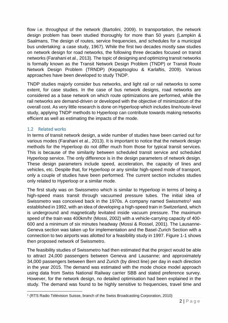
The first study was on Swissmetro which is similar to Hyperloop in terms of being a
high-speed mass transit through vacuumed pressure tubes. The initial idea of
Swissmetro was conceived back in the 1970s. A company named Swissmetro1 was
established in 1992, with an idea of developing a high-speed train in Switzerland, which
is underground and magnetically levitated inside vacuum pressure. The maximum
speed of the train was 400km/hr (Mossi, 2002) with a vehicle-carrying capacity of 400-
600 and a minimum of six minutes headway (Mossi & Rossel, 2001). The Lausanne-
Geneva section was taken up for implementation and the Basel-Zurich Section with a
connection to two airports was allotted for a feasibility study in 1997. Figure 1-1 shows
then proposed network of Swissmetro.
The feasibility studies of Swissmetro had then estimated that the project would be able
to attract 24,000 passengers between Geneva and Lausanne; and approximately
34,000 passengers between Bern and Zurich (by direct line) per day in each direction
in the year 2015. The demand was estimated with the mode choice model approach
using data from Swiss National Railway carrier SBB and stated preference survey.
However, for the network design, no detailed optimisation had been explained in the
study. The demand was found to be highly sensitive to frequencies, travel time and
1 (RTS Radio Télévision Suisse, branch of the Swiss Broadcasting Corporation, 2010)

3 | P a g e
fares (Georg, 1999). Despite a few feasibility studies, the project could not be
developed further, due to higher initial investment requirements, lack of financial
support from the government and less profitability (estimated IRR of around 3%). This
led to the dissolution of the company in 2010 (RTS Radio Télévision Suisse, branch of
the Swiss Broadcasting Corporation, 2010).
Figure 1-1 Swissmetro network (L’ association Pro Swissmetro, 2015)
Usually, the cost of elevated networks is lesser compared to underground networks.
Likewise, construction of an elevated Hyperloop might require lesser initial investment
compared to the Swissmetro. The initial investment cost of Basel-Zurich pilot line was
estimated to be 67 million CHF/km, while the operating cost for 40 years was 79 million
CHF on the basis of 2002 rates (Mossi & Vuille, 2002). The Hyperloop Alpha estimates
an initial investment of 10.60 million CHF/km for the infrastructure and vehicles
between Los Angeles and San Francisco as per 2013 rates (SpaceX, 2013). However,
a detailed comparison needs to be made as the characteristics of both modes differ in
many aspects. Table 1-1 compares the technical specifications of Swissmetro and
model of the Hyperloop One system (Jufer, 2018) (SpaceX, 2013). From the table, it
can be observed that the Hyperloop system is a tuned version of Swissmetro in terms
of technical parameters (e.g. vehicle capacity, acceleration, speed and many more).
Another similar study for the Hardt Hyperloop System was carried out by Beets A.D.J
(2019). Though the study focused on the line-level approach from Berlin to Paris, it is
still relevant to this research. The study applied Minimum Spanning Tree (MST)2
between Berlin and Paris connecting major cities along the line for network generation.
The author developed a mixed-integer linear problem in order to optimise capacity and
fleet size for the line. A part of the study, also focused on demand estimation, for which
2 Minimum spanning tree is a solution in graph theory that generates network in a way that overall network has minimum weight and no cycles are present in the network.

4 | P a g e
a multinomial logit model was applied. However, weights of the variables in the utility
functions were chosen arbitrarily. This was mainly due to unavailability of the actual
estimates or insufficient literature.
A recently published study was carried out by Delft Hyperloop. van Leeuwen, et al.
(2019) developed a European Hyperloop network connecting the 48 major European
cities with 51 links in their Hyperloop network. For demand estimation, the authors
used the European Passenger Database of 2017 and scaled up for the year 2040.
Different scenarios were assumed based on the growth in passengers. The highest
growth and lowest growth were considered for the design of the network without
applying a mode choice model. The direct demand for air passengers was used as
Hyperloop demand. The link flows were assigned through the ratio of shortest path
distance and the actual distance between the cities. Similarly, no thorough optimization
was performed in the study.
Table 1-1 Technical parameters - Swissmetro and Hyperloop (Jufer, 2018) (SpaceX, 2013)
No Parameters Swissmetro Hyperloop One
1 Grade level Underground Elevated
2 Tunnel Type & Diameter Double tunnel, 5m Double tube, 2.3m-3.3m
3 Vehicle Diameter 3.2m 1.38m-1.98m
4 Air Pressure 7% 1%
5 Technology for power Magnetic levitation Air cushion levitation
6 Guidance Magnetic Guidance Air cushion guidance
7 Motors Brushless DC linear motor Linear Induction Motor
8 Energy in Vehicle contactless Batteries
9 Max. Acceleration 0.13 times g 1 times g
10 Vehicle Mass 50-100 tons (200-400 pass) 15 tons for 28 pass
11 Max. Power 6MW for 400 pax
50MW for 28 pax
12 Power/kg 60 W/kg 3300 W/kg
13 Max. Speed 432 km/hr 1200 km/hr
14 Vehicle length 50-100 m 30 m
15 Min. Headway 6 min 6 min
In all the previously mentioned studies, high-speed transit networks have been
developed applying MST and the flows have been assigned to the links with the
shortest path. A few line-based studies also have been developed for the Hyperloop,
e.g. Hyperloop Alpha (2013) between Los Angeles and San Francisco which estimates
the overall cost of the lines; the pre-feasibility study of Stockholm-Helsinki also
estimates the demand and the cost of the line (KPMG Sweden Inc., 2016). However,
these studies do not optimise the lines or analyse the societal impacts of the system
either. Thus, none of the previous studies shows any thoroughly applied optimization
or detailed assessment for the Hyperloop network so far.
1.3 Problem context In general, TNDP consists of five steps: (i) Designing routes; (ii) Setting frequencies;
(iii) Developing timetables; (iv) Scheduling buses (vehicles); and (v) Scheduling drivers
(Ceder & Wilson, Bus network design, 1986). These methods are largely applicable to

5 | P a g e
bus networks, where the road network is a base network. However, in the case of Rail
one more step is added beforehand, i.e. network generation. Network generation
designs the network structure or defines the network elements i.e. nodes and links.
From the perspective of TNDP, network design has been solved using different
objectives that can be applied to different modal networks e.g. car, bus, rail, ferry etc.
Largely, these objectives can be summarised into six categories (Black, 1995; Fielding,
1987; van Oudheusden, Ranjithan, & Singh, 1987), mapped to three further
perspectives (van Nes & Bovy, Importance of objectives in urban transit network
design, 2000). as shown in Table 1-2. Table 1-2 Type of objective functions
No. Categories Perspective
1 User benefit maximization User
2 Operator cost minimization Operator
3 Total welfare maximization User, operator and public authority
4 Capacity maximization Operator and public authority
5 Energy conservation protection of the environment
Public authority
6 Individual parameter optimization User
The user benefit maximization covers travel time savings, while the operator’s
perspective focuses on reducing, the operational costs. The user benefit maximization
does not take into account the cost aspects of infrastructure or the operator. The
authority, in general, is interested in increasing societal welfare, the capacity of the
lines or reducing energy consumption and environment emissions. The individual
parameter optimization includes line-specific transfers, transfer wait time or
accessibility improvement. These objectives were categorised into three perspectives
further This categorisation affects the network configuration. For example, van Nes et
al. (2000) defines variables like stop spacing and line spacing for urban transit
networks with users’ and operators’ perspectives. As for the Hyperloop system, overall
societal benefits (i.e. ex-ante evaluation) needs to be assessed initially, before the
implementation. And also, the category of total welfare maximization can be interpreted
as minimisation of total cost i.e. infrastructural cost, operational cost and user cost.
This can be considered as an objective function for the Hyperloop network design.
To design the network, based on the suitable category of objectives, a scenario-based
approach (SBA) can be implemented as well. Vittins et al. (2017) in their study on
“Extraction and evaluation of transportation network grammars for efficient planning
applications” explain the importance of a scenario-based approach. The SBA
generates different scenarios under the defined set of rules for the inputs of the model.
This can be with same or different objective functions. The SBA determines the future
scenario with the highest return under given budget constraints from a set of previously
generated alternatives. The advantage is that a direct comparison can be made
between these alternatives as the same rules will apply to all the alternatives in terms
of evaluation. However, a drawback is that long-term impacts cannot be assessed, for
which a separate qualitative or a quantitative analysis has to be carried out (Vittins et
al., 2017). This can lead to the generation of suboptimal design for the future. Thus, in
order to compare the different alternatives of Hyperloop network, SBA can be
implemented as well.

6 | P a g e
1.4 Research gap After looking at the related works and problem context, it can be observed that there is
a research gap in the area of designing and impact evaluation of a new transit system
such as Hyperloop. Though previous studies considered the cost for the network
design, demand could not gain attention in the design process. Similarly, in the cost
aspect of the network, a few attempts have been made to estimate the real cost of
infrastructure by neglecting evaluation of societal impacts. The studies only show
discussion of these gains or benefits of implementing such huge infrastructure
qualitatively (SpaceX, 2013). This defines the research gap in the quantification of the
societal benefits of the Hyperloop system. Before implementing the overall system, an
ex-ante evaluation is therefore required. This study can contribute towards the
methodological implementation of existing ex-ante evaluation guidelines as well as
design.
The overall idea of network design is to develop a solution following a specific objective
in order to perform under certain standards. This can be useful in many ways, with
research in designing networks:
• Hyperloop network, providing an understanding of network structure in terms of
links and nodes.
• Routes and frequency; an indication of overall travel time benefits and the fleet
size required for the network can be attained.
• Required resources for the same can be estimated.
Similar to most of the ex-ante evaluation, this research can be used to evaluate the
different scenarios for the same. Though this research does not contribute towards a
methodology for optimisation, results can spur discussion for further improvements in
terms of network parameters. Also, the effect of the Hyperloop network can be studied
largely on the overall transport network, which will essentially be helpful for the ex-ante
evaluation of the system and gives an indication of viability.
1.5 Research question From the aforementioned research gap, the following research question has been
derived.
“How can a Hyperloop network be designed based upon the determinants of the
costs benefits analysis?”
The research question aims to find the maximum benefit-cost (B/C) ratio, which has
been used as an indicator of ex-ante evaluations. The Hyperloop network scenario is
compared with a no Hyperloop network scenario.
Please note that:
• The research question does not focus on the estimation of the demand in terms
of the mode choice model. The estimation of demand requires detailed choice
modelling. Hence, the estimation of weights variables in the utility function for
Hyperloop needs to be studied separately as a more thorough research
exercise.

7 | P a g e
• Making nodes variable makes the research complex. Considering the given time
frame, nodes (stations) are considered to be fixed or predefined for the network.
• The overall network development is considered as a sequential procedure. This
is also a pragmatic choice considering the limitation of computational time.
Figure 1-2 shows the procedure for the overall network design, which can be
divided into three steps. The first step ‘Network Generation’ defines the links
between the nodes. Further, the second step defines the routes and frequency
for the network, while the third step performs the detailed assessment of the
network designs.
Figure 1-2 Research flow
Considering the overall process of network design, the sub-questions in this study can
be summarised as below.
1. What are the inputs required for the network design of a Hyperloop system?
2. What are the methods to design/optimise transit networks such as Hyperloop?
3. What is the feasible set of links in a Hyperloop network with respect to benefit
to cost (B/C) ratio?
4. Which is the optimal set of routes for the Hyperloop network generated in the
previous sub research question? What are the frequencies and number of
vehicles required for the respective lines?
5. What is the B/C ratio of the Hyperloop network generated in the previous sub-
research question?
6. To what extent is the B/C ratio of the Hyperloop network sensitive to its design
inputs?
Sub-research question one is directed towards the input preparation for the overall
design process. Sub-research question two is a methodological question. This tries to
define the method to answer the main research question from the literature review.
Sub-research question three is part of network generation, while sub-research
question four defines the lines in the network with frequencies and the required number
of vehicles. This will also give an indication of operational cost. At last, sub-research
questions five and six concerns the post result analysis. Questions two, three, four, five
and six are in a sequential manner. Answering each of them will help to answer the
subsequent one.
1.6 List of assumptions The list of assumptions used in network design later in this report is presented below.
These assumptions are further explained in the subsequent chapters.
Network GenerationStep:1
•Network Route Design
•Network Frequency Setting
Step:2•Cost-Benefit
Analysis
•Sensitivity Analysis
Step:3

8 | P a g e
1.6.1 Vehicle
• The speed of the vehicles is assumed to be 1000 km/hr for the links >30 km,
while for the shorter links, the maximum speed is assumed to be 500km/hr.
• The value of acceleration and deceleration is considered to be 0.5G.
• The capacity of the vehicle is assumed to be 50 sitting passengers per vehicle
• The minimum headway of 90 seconds has been assumed considering the time
of passengers moving in-out and time required for fastening their seat belts.
1.6.2 Network & service
• Links are considered to be non-planar i.e. intersecting links do not generate a
node.
• The nodes are fixed.
• The demand is assumed to be fixed throughout the design process.
• All the links are considered bi-directional.
• No capacity restrictions are considered while generating the network.
• No overtaking possibilities over the lines are considered. This leads to a line
capacity of 2000 passengers per hour per direction.
• The networks are required to be connected.
1.7 Outline Thus, the research question and bases for the research have been defined. Chapter 2
defines the problem mathematically and describes the methodology with a detailed
literature review, whereas chapter 3 is case-specific where inputs for the model have
been developed. Chapter 3 answers the sub-questions one as well. Chapter 4
discusses the results and performs the cost-benefit analysis with the case-specific
guidelines, and chapter 5 concludes the study by discussing recommendations and
limitations. As described here, Figure 1-1 shows the flow of the research along with
the chapter number indicated for the thesis.
Figure 1-3 Outline of the project
1. Introduction
2. Methodology
3. Experimental setup
4. Results
5. Conclusion

9 | P a g e
2 Methodology
This chapter describes the study approach developed to answer the main research
question. Also, in order to define the approach, it is required to identify the methods
that are being practised in the field of network design and optimisation. The chapter
starts with section 2.1 describing and reviewing the previously implemented design
and optimisation approaches. This helps to answer the sub research question two.
Section 2.2 describes the adapted study approach, in all the stages of design i.e.
network generation, route design and assignment procedure. This will answer the sub
research question two.
2.1 Selecting the modelling approach As mentioned, this section identifies the methods adopted and helps to formulate the
design method for the current design problem through literature review. Transit
network design problem (TNDP) has been defined as a complex and difficult to solve
problem. It has been studied for more than five decades. The current section captures
important studies that have dealt with this topic previously. Kepaptsoglou et al (2009)
compiled more than 60 studies in the field of TNDP in a detailed literature review.
Farahani et al. (2013) also carried out a literature review extending the works of
Kepaptsoglou et al (2009). However, the categorisation of the problems is different in
all of the studies. As mentioned in the background section of the document, the
problem solution is largely classified into two categories, i.e. Conventional and
Heuristic (Baaj & Mahmassani, 1991). This section explains both classifications from
the literature.
Conventional methods include analytical approach and mathematical programming
(Kepaptsoglou et al., 2009). Farahani et al. (2013) defined them as exact or
mathematical methods. Analytical methods identify relationships between the
components of transit networks (Ceder et al., 1986; van Oudheusden et al., 1987;
Chakroborty, 2003). Generally, these solutions are developed for local optimisation
based on mathematical properties (Kepaptsoglou et al., 2009). Earlier applications of
these methods can be observed in small networks (Holroyd, 1965; Hurdle, 1973;
Byrne, 1976; Byrne, 1975; Kocur & Hendrickson, 1982). As these methods are
considered to be inefficient for large networks, they were applied by some of the
researchers to medium size networks (Tsao & Schonfeld, 1983; Chang & Schonfeld,
1993; Chang & Schonfeld, 1993a; Spacovic & Schonfeld, 1994). All these applications
were mainly on bus route network design problems with the aforementioned objectives
in section 1.3. These methods are considered to be simple and easy to implement for
generating small networks. Branch and bound method is a good example of it. Ceder
(2001) mentioned that analytical methods can be used for the policy evaluation and to
estimate the values for design parameters approximately, not for the complete design.
The aforementioned Delft Hyperloop Student Team study is based on the analytical
approach.
The other approach is to implement mathematical programming, which is based on
solving non-linear equations. These methods are considered to be efficient for non-
linear problems and can be used for solving large networks, whereas analytical
methods are incapable of doing the same (Tom & Mohan, 2003). The first applications

10 | P a g e
of the same were given by van Nes, Hamerslag & Immers (1988) and Baaj &
Mahmassani (1991). These were linear models. The first non-linear models were given
by Constantin & Florian (1995) and Russo (1998). However, these studies did not
consider routes as decision variables. van Oudheusden et al. (1987) gave an important
study with the same approach, where routes were considered as a decision variable.
However, the study was based on the plant location problem rather than public transit
problem. Some researchers have mentioned the disadvantages of these conventional
methods for the route generation. However, these remarks were largely based on the
generation of bus routes on large road networks. Chakroborty (2003) also drew
attention to the fact that mathematical programming is inadequate to represent the
problem to a realistic extent. Tom & Mohan (2003) also noted that these methods are
useful for theoretical interest only. However, these methods have also been
implemented in other networks like Rail Networks or Ferry Design Networks (Bell et.
al., 2019).
The other category of the optimisation methods includes Heuristic Methods and Meta-
heuristic Methods. These methods generate a candidate set of routes based on some
defined criteria, followed by generating either a subset of optimal routes or improving
previously generated routes by adding or removing network elements (Farahani et al.,
2013). The heuristic methods are problem-specific algorithms while the meta-heuristic
algorithms are globally accepted like Genetic Algorithm, Simulated Annealing or
Ant/Bee-Colony Algorithm. One of the important and initial works pertaining to this
approach was given by Mandl C. E. (1980) for route designing and frequency setting.
The algorithm was based on the shortest path between a pair of terminals serving the
maximum number of Origin-Destination (OD) pairs. The idea was to have minimum
travel time by reducing the waiting time and transfers. These methods are efficient in
terms of computational power and can be implemented on large networks effectively
(Farahani, et al., 2013). However, methods do not give global optimal solutions but
provide one of the nearly optimal solutions fitting into criteria (Kepaptsoglou, et al.,
2009). These methods have largely been implemented for the last three decades. They
require a thorough understanding of the problem as a decision is in each step. This will
also decide the following step. The heuristic methods have been given lesser attention
compared to meta-heuristic methods.
As mentioned before, meta-heuristic methods include partly predefined algorithm. In
general, all the meta-heuristic algorithms have been implemented in other fields before
being implemented in the field of transportation. These methods do not require detail
mathematical formulation of the algorithm. Among these methods, the most widely
adopted approach is Genetic Algorithm (GA). One of the initial applications of GA in
TRNDP was given by Chien S. et al. (2001). The authors optimise bus routes and their
headways by minimising the total cost. GAs have hence been used to determine
routes, fleet size, and frequency with different objective functions. Being widely
adopted GAs, some contradictory observations have been noted by authors in terms
of the quality of results. Many researchers have also noted that GAs perform worse
than Simulated Annealing (SA) or Ant Colony Optimization (ACO) (Fan & Machemehl,
2006). Since the last decade, another approach known as the Ant Colony
Optimization/Bee Colony Optimization has started to be practised in TNDP. One of the
initial applications of ACO was given by Hu et al. (2005) in bus transit networks to

11 | P a g e
optimize the routes and headways with the objective of maximising the passenger flow
in the network. In a similar way, ACO has been used for route optimization, optimal
station locations, headways and frequency with different and multi-objective functions.
However, it has been noted that ACO takes longer computational time. There have
been also attempts to implement the hybrid meta-heuristic approach. One of the initial
studies noted that integrating SA and GA gave better results than GA only (Zhao &
Zeng, 2007). Zhao et al. (2007) combined Tabu Search method & SA instead of GA
and observed that the results are good in a considerable amount of time. To reduce
the computation time for the convergence, Vitins, B. (2014) also combined ACO and
GA, as the former had greater accuracy and the latter had shorter computational time.
The algorithm was used to optimise the road network in Switzerland in order to
minimise the user cost. The author also found that integrated approach outperforms
GA, in terms of accuracy.
From the above-mentioned studies and methods for transit network optimization, the
characteristics of the methods are summarized as per Table 2-1. The table shows five
characteristics of each method starting from complexity, followed by large network
suitability, computational time, quality of results, level of detail and type of optimisation.
The categorisation of the methods is followed from Kepaptsoglou et al. (2009). The
properties are taken up from the literature. This also includes the interpretation of the
author, which can be subjective to some extent. The characteristics of complexity,
quality of results and level of detail are measured in high, medium and low, while large
network suitability yes, medium and no. The optimisation has been distinguished
between local and global. From the categories, meta-heuristics found out to be the
best except in the quality of results. This is due to less accuracy of GA and ACO.
Table 2-1 Optimisation methods' characteristics
Method Complexity
Large Network
Suitability
Time for Computation
1
Conventional Analytical Low No High
2 Mathematical Programming
High Medium Medium
3 Heuristic
Heuristic Medium Medium Low
4 Meta-heuristic Low Yes Mixed
Method
Quality of Results
Level of Detail
Optimisation
1
Conventional Analytical High Less Local
2 Mathematical Programming
High Medium Mixed
3 Heuristic
Heuristic Medium High Global
4 Meta-heuristic Low Medium Global
The above-mentioned studies show single method implementation or hybrid to some
extent. Often heuristic methods are merged with mathematical programming in order
to solve TNDP. This has been developed through bi-level optimisation in which the
upper-level optimisation of route configuration has been carried out with mathematical
programming, while lower-level optimisation with meta-heuristic algorithms. Fan &
Machemehl (2011) used a genetic algorithm for the bi-level optimisation. The upper-

12 | P a g e
level optimisation was performed with GA in order to develop the transit network with
minimum operational cost, while the lower level was based on mathematical
programming in order to generate routes and frequency with minimum user cost. Also,
in this approach, the studies show sequential and simultaneous approaches for
network generation and route design. It has been noted that the latter gives better
results in terms of quality.
2.2 Adapted modelling approach As mentioned in the previous chapter the current network design is carried out in two
stages. The first one includes network generation, while the second one route design
and frequency setting. In the current section, the main steps of each stage are
explained. Figure 2-1 shows the main steps of the overall research methodology.
Figure 2-1 Research methodology
Considering the characteristics of Hyperloop, for the network generation heuristic
approach can be adopted. This is mainly because of smaller Hyperloop networks.
Since higher mode speed and larger distance requirement for acceleration will lead to
larger stop spacing. This will lead to a smaller size of the networks. Considering the
higher cost for station operation, the network is also required to be connected, as
stated in one of the assumptions of the study. This will reduce the user cost of
transferring to other modes, which will lead to increased benefits.
As mentioned in the research gap, the current study also aims to evaluate the societal
cost and benefits of the system, B/C ratio is considered as a performance indicator of
the network generation part, while number of transfers which is part of user cost has
been considered as an objective function to be minimised for the route design.
However, in transport networks benefits are mainly dominated by user cost i.e. travel
time savings compared to other benefits like externalities (environmental emissions,
noise, accident cost etc.) and cost are mainly dominated by infrastructure and
operational & maintenance cost, those have been only considered for the optimisation.
This is explained in detail in the subsections.
2.2.1 Network generation
Beets A.D.J. (2019) adopted MST for the network generation. Demand was not part of
the consideration for the network generation. However, this approach does not ensure
the maximisation of benefits. The current study also considers the demand for the
network generation. This leads to the development of two approaches;
Generation of set of candidate links for route design
Network generation
Defining routes and respective
frequencies
Route design
and frequency
setting
Post results analysis:
Cost Benefit and
Sensitivity
Assignment & Network
performance evaluation

13 | P a g e
(i) Additive approach, in which the initial network is developed based on MST
and further improvements in the links are made based on the travel time
savings and cost,
(ii) The deductible approach in which initially fully connected network is
generated and links are deleted until tree in the network is reached or B/C
reaches less than one.
The algorithms are initially used in ferry network design problem with different objective
functions. by Bell et al. (2019). However, apart from objective function, adding-
removing criteria and convergence criteria were different in the study. The algorithms
were named as Link Swapping algorithm and Link Deletion algorithm. Both of the
algorithms are heuristic in nature. The similar nomenclature is followed in the current
study as the core idea remained the same.
The idea of network generation algorithm is to identify the links that are feasible i.e.
B/C ratio is ≥1. However, it may be possible that this will generate redundant links since
the gains from travel times are significantly higher because of the very high speed of
the mode. This will add a step after route design for the adjustments i.e. removal of
redundant links.
it is also important to note that demand is considered to be fixed throughout the
process. Also, for the network generation process, only infrastructure cost for the cost
part, while for the benefits it is assumed that no transfer, waiting and stop time will be
required.
For both the network generation algorithms, the set of nodes; travel times of existing
networks, unit infrastructure cost of links and stations cost; and OD matrix are the
inputs required to feed. In the subsections explain both the approaches in detail. Both
the algorithms generate a feasible set of links along with the B/C ratio for the network
with the considered costs and benefits. The B/C ratio is calculated by taking a ratio of
travel time savings {(i.e. existing network total travel time and Hyperloop network travel
time)* VoT} / infrastructure cost. The following section explains the main steps of the
link swapping algorithm and link deletion algorithm.
The following sub-section explains both the approaches with an example and pseudo-
code developed in R syntax.
2.2.1.1 Link swapping approach
The general steps of the algorithm are shown in Figure 2-4. The current section
explains the main steps of the link swapping algorithm. The algorithm starts with the
minimum cost network and develops the network further towards the direction of
increasing benefits. The steps of the algorithm as follow:
1. After feeding the inputs, the algorithm is initiated with the MST (set of links E)
based on the cost of the network. In this step further, travel times of each link
will be calculated based on the parameters mentioned in the assumption
section. Based on this travel time, the flow will be assigned to each link. This
will help to calculate the B/C ratio(F) of the network.

14 | P a g e
Figure 2-2 shows an example of the link swapping approach. Sub-figure (1)
develops the network in a way that the overall structure has minimum cost and
no cycles in the network.
2. In the first iteration, from the non-chosen links (E’), maximum demand OD pair
will be connected via a direct link. This will lead to reassigning the flow and
recalculating the B/C ratio (F’).
3. If the calculated B/C ratio (F’) remains greater than one, further links will be
added as per the conditioned mentioned in step 2, until the B/C ratio reduces to
less than one.
In the sub-figure (2), link AD is added provided OD pair AD had the maximum
direct demand.
4. If the calculated B/C ratio (F’) drops below 1, a minimum flow link will be
removed, while making sure that the graph remains connected. This will again
lead to re-assigning of flow and recalculation of the B/C ratio.
The B/C ratio of the network still remains above 1. Therefore, another maximum
demand link AC is added. However, after re-assigning the demand in the
network the overall B/C ratio of the network drops below 1.
5. Step two, three and four are followed in iteratively, until added link and the
removed link are the same in the consecutive iterations.
This will lead to the removal of the minimum flow link AB.
6. If the added link and removed links are the same in consecutive iterations, the
algorithm will be stopped. At this point, the network will be considered as an
output along with the B/C ratio.
For the current example, the B/C ratio goes above one after removal of AB link.
This will lead to finding another maximum direct OD pair. This turns out to be
AB again and in the next step, AB is also removed. So, this converges the
algorithm.
Since the network starts with minimum cost, it will have the highest B/C ratio. This
approach is contradictory to the following approach. The algorithm identifies the
local optima.
The pseudo code developed for the approach in R syntax is shown here in the box.
The pseudo code shows only iterative procedure.
# get minimum spanning tree matrix, assign demand, and calculate bca ini_dist_mst <- minimum.spanning.tree(ini_dist_g) ini_dist_mst <- assign_demand(ini_dist_mst, nr_node, demand_mat_net_gen) plot(ini_dist_mst) bca_table <- matrix (c("0", "initial_mst", "NA", calculate_simple_graph_bca(ini_dist_mst, vot, ett, infra_cost, stations_cost)), ncol = 6) # iterative process starts here new_dist_g <- ini_dist_mst new_links <- NULL iter <- 0 repeat {iter <- iter + 1 print(iter) # add direct link for the link with maximum flow which is not on graph already # on the condition that the link adds on the old bca

15 | P a g e
# the function will loop until a link is found repeat {new_dist_g <- add_max_demand_link(ini_dist_g, new_dist_g, if(!is.null(new_links)) gsub(", ", "|", new_links) else NULL, nr_node, demand_mat_net_gen) link_added <- paste(new_dist_g[[2]], collapse = ", ") new_links <- c(new_links, paste(new_dist_g[[2]], collapse = ", ")) bca <- calculate_simple_graph_bca(new_dist_g[[1]], vot, ett, infra_cost, stations_cost) bca_table <- rbind(bca_table, c(iter, "link_added", link_added, bca)) new_dist_g <- new_dist_g[[1]] if(bca[[3]] < 1) break } repeat { # remove minimum flow link # on the condition that the graph stays connected and bca becomes higher than 1 # if the conditions are not met then the link will not be removed #and link with second minimum will found etc until conditions are met new_dist_g <- remove_min_demand_link(new_dist_g, vot, ett, infra_cost, stations_cost, nr_node, demand_mat_net_gen) link_removed <- paste(new_dist_g[[2]], collapse = ", ") new_dist_g <- new_dist_g[[1]] bca <- calculate_simple_graph_bca(new_dist_g, vot, ett, infra_cost, stations_cost) bca_table <- rbind(bca_table, c(iter, "link_removed", link_removed, bca)) # move to another iteration of adding/removed # until the link added is the same as link removed if(bca[[3]] > 1) break } if(link_added == link_removed) break} # plot final graph
plot(new_dist_g)
Figure 2-2 An example of link swapping
Figure 2-3 An example of link deletion

16 | P a g e
Figure 2-4 Link swapping algorithm
Figure 2-5 Link deletion algorithm
2.2.1.2 Link deletion approach
The general steps of the link deletion algorithm are shown in Figure 2-5. This algorithm
starts with the maximum connected network and progresses towards reducing the
network. The main steps from the figure are explained below:
1. After feeding the inputs, the algorithm starts with connecting all the nodes to
each other. This will generate a fully connected network. Once the network is
generated the flow will be assigned to the links via shortest paths and
subsequently, B/C ratio will be calculated for the graph based on the travel times
calculated according to parameters mentioned in the assumptions.

17 | P a g e
Figure 2-3 shows an example of the link deletion approach. In the first step, as
it can be seen from the sub-figure (1), al the nodes are connected, and demand
is directly assigned.
2. In the next step, a minimum flow link will be removed. This will lead to the re-
assigning of the flow and re-calculation of the B/C ratio.
As sub-figure (2) shows in the next step, link BD is removed since the link has
minimum demand and B/C ratio is above one.
3. Step two will be followed iteratively until the network reaches the tree structure
or the B/C ratio is reduced to less than one.
As sub-figure (3), shows the link AB is removed since it has minimum demand
after re-assigning the demand of the network.
4. If the network reaches to the tree structure, the same iteration results will be
stored, and the network will be considered as an output.
In further, the link AC could be removed. However, this led to reducing the B/C
ratio of less than one. Therefore, link AC is restored in the network.
5. If the B/C ratio of the network reaches to one, one iteration previously, results
will be stored, and the network structure will be considered as output.
This approach of link deletion tries to identify the global optimum. The algorithm starts
with the minimum B/C ratio and progresses towards the improving B/C ratio of the
network.
The pseudo code developed for the approach in R syntax is shown here in the box.
The pseudo code shows only iterative procedure: # export adjacency matrix of initial graph write.csv(as.matrix(get.adjacency(ini_dist_g)), "AdjacencyMatrixFullGraph_m2.csv") # initial bca table to be exported bca_table <- matrix(c("0", "initial_fg", "NA", calculate_simple_graph_bca(ini_dist_g, vot, ett, infra_cost, stations_cost)), ncol = 6) # iterative process starts here new_dist_g <- ini_dist_g new_links <- NULL iter <- 0 repeat { iter <- iter + 1 print(iter) # remove minimum flow link # on the condition that the graph stays connected # if the conditions are not met then the link will not be removed #and link with second minimum will found etc until conditions are met new_dist_g <- remove_min_demand_link_m2(new_dist_g, vot, ett, infra_cost, stations_cost, nr_node, demand_mat_net_gen) link_removed <- paste(new_dist_g[[2]], collapse = ", ") breaks <- new_dist_g[[3]] new_dist_g <- new_dist_g[[1]] bca <- calculate_simple_graph_bca(new_dist_g, vot, ett, infra_cost, stations_cost) bca_table <- rbind(bca_table, c(iter, breaks, link_removed, bca)) # break if network gets disconnected or if network becomes a tree if(breaks %in% c("stop_removing_tree", "stop_removing_bca")) break} # plot final graph plot(new_dist_g)

18 | P a g e
Both of these approaches identify the networks with the feasible set of links i.e. B/C
ratio above one. This network will be considered as an input for the next route design
algorithm. The following sub-section explains the route design stage.
2.2.2 Network route design and frequency setting
The networks generated in the previous step are taken up for the route design. As
mentioned previously, the route design algorithm is based on Mandl C.E. (1980)
approach. This is one of the earliest applications of Heuristic methods in TNDP. The
algorithm optimises the number of transfers on a set of lines.
As there are two different networks will be generated from the previous stage, the route
designing algorithm will be applied to both the networks. Figure 2-6 shows the general
steps for the algorithm. The main inputs for the algorithm will be a network with OD
demand matrix. The general steps are described below:
1. In the first step, the algorithm identifies the longest shortest path of the network
and saves it as a line. Once a line is selected, the selected links and nodes are
deleted from the network while ensuring that the rest of the network is
connected.
Figure 2-7 shows an example of the route design3. As per the longest shortest
paths of the network, BED and AEC are two lines generated from the network.
2. With the same conditions, the second line is identified. This process is followed
iteratively until all the nodes are covered at least by a line. Here, while selecting
a line, one must make sure that in the same line a node is not visited twice. This
avoids cycles in a line.
3. Once a set of lines is defined, the maximum number of transfer point is identified
between each pair of lines via assigning the flow on each line.
This identifies E as the maximum number of transfer point in the given set of
lines.
4. In the next step, the number of transfers will be calculated on the transfer node.
5. In this step, the portions of the lines are interchanged from the identified
maximum transfer point in the previous step. This process is iteratively followed
for all the possibilities.
This will lead to a generation of a different combination of lines, like AED & BEC
and AEB & CED as shown in sub-figure (3) and (4).
6. The set of lines with the minimum number of transfers will be considered as an
output of the algorithm.
7. On this set of lines, the load profile is plotted for each line. Based on the
maximum load on the line, the frequency of each line will be calculated. This will
also help to calculate the number of vehicles required in combination with cycle
time.
3 This example is not in continuation with the previous example.

19 | P a g e
Figure 2-6 Route design algorithm
The algorithm gives routes with assigned frequency (also fleet size) as output. It
generates the routes based on the shortest path initially which minimises the operator’s
cost and proceeds towards reducing user cost by minimising the number of transfers.
It is also important to note that the algorithm initially does not consider overlapping
routes, which makes heuristic nature of it.
Figure 2-7 An Example of route design
The pseudo-code developed in R syntax for the routes is shown in the box on the next
page:

20 | P a g e
get_ids_with_single_edge <- function(graph) { ids <- NULL all_nodes <- names(unique(V(graph))) for(i in all_nodes) { if(length(which(as.vector(get.edgelist(graph)) == i)) == 1) ids <- c(ids, i) } return(ids)} # get nodes with maximum transfer points get_node_with_maximum_transfer <- function(graph) { temp <- table(as.vector(ends(graph,E(graph)))) return(names(which(temp == max(temp))))} swap_all_lines <- function(line_i, line_j, nodes) { interchange_i <- which(line_i %in% line_j & line_i %in% nodes) interchange_j <- which(line_j %in% line_i & line_j %in% nodes) if(interchange_j[length(interchange_j] == length(line_j) | line_i[length(line_i)] == line_j[length(line_j)] | !all(line_1[which(line_2 %in% line_1)] == line_2[which(line_2 %in% line_1)])) { line_2 <- rev(line_2) interchange_2 <- which(line_2 %in% line_1 & line_2 %in% nodes) } line_mod_11 <- c(line_1[1:(interchange_1[length(interchange_1)])], line_2[(interchange_2[length(interchange_2)] + 1):length(line_2)]) line_mod_12 <- c(line_2[1:(interchange_2[length(interchange_2)])], line_1[(interchange_1[length(interchange_1)] + 1):length(line_1)]) if(line_mod_11[1] == line_mod_11[length(line_mod_11)]) line_mod_11 <- line_1 if(line_mod_12[1] == line_mod_12[length(line_mod_12)]) line_mod_12 <- line_2 return(list(line_mod_11, line_mod_12))} # get all the scenarios of lines by swapping ends of common nodes get_all_lines_scenarios <- function(lines, max_transfer_pts) { scenarios <- list(lines) for(i in 1:(length(lines) - 1)) { for(j in (i+1):length(lines)) { lines_mod <- swap_two_lines(lines[[i]], lines[[j]], max_transfer_pts) lines[[i]] <- lines_mod[[1]] lines[[j]] <- lines_mod[[2]] scenarios <- c(scenarios, list(lines)) } } return(scenarios)} # get load profile for lines get_load_profile <- function(graph, line, demand_matrix) { temp <- rep(line, each=2)[-1] temp <- temp[-length(temp)] line_edges <- get.edge.ids(graph, temp) sub_g <- subgraph.edges(graph, line_edges, line_edges) sub_demand <- demand_matrix[which(rownames(demand_matrix) %in% names(V(sub_g))), which(colnames(demand_matrix) %in% names(V(sub_g)))] sub_g <- assign_demand(sub_g, nrow(sub_demand), sub_demand) return(sub_g)} get_load_profiles <- function(graph, scenarios, demand_matrix) { d12 <- data.frame() for (i in 1:length(scenarios)) { for (j in 1:length(scenarios[[i]])) { temp <- get_load_profile(graph, scenarios[[i]][[j]], demand_matrix) d12 <- rbind(d12, data.frame(scenario = i, line = j, line_name = paste0(scenarios[[i]][[j]], collapse=","), edge = as_ids(E(temp)), load_profile_dir1 = E(temp)$assigned_demand_d1, load_profile_dir2 = E(temp)$assigned_demand_d2)) }}return(d12)} # get frequency of each line get_line_freq <- function(graph, line, demand_matrix, veh_capacity) { lp <- get_load_profile(graph, line, demand_matrix) d1 <- which.max(E(lp)$assigned_demand_d1) d2 <- which.max(E(lp)$assigned_demand_d2) m <- which.max(c(E(lp)$assigned_demand_d1[d1],E(lp)$assigned_demand_d2[d2])) if(m == 1) { return(data.frame(line = paste0(line, collapse = ","),

21 | P a g e
link_with_max_directional_demand = as_ids(E(lp)[d1]), assigned_demand = E(lp)$assigned_demand_d1[d1], freq = E(lp)$assigned_demand_d1[d1] / veh_capacity)) } else if(m == 2) { return(data.frame(line = paste0(line, collapse = ","), link_with_max_directional_demand = as_ids(E(lp)[d2]), assigned_demand = E(lp)$assigned_demand_d2[d2], freq = E(lp)$assigned_demand_d2[d2] / veh_capacity))}} get_lines_freq <- function(graph, scenarios, demand_matrix, veh_capacity) { lines_freq <- data.frame() for(i in 1:length(scenarios)) { for(j in 1:length(scenarios[[i]])) { lines_freq <- rbind(lines_freq, cbind(scenario = i, get_line_freq(graph, scenarios[[i]][[j]], demand_matrix, veh_capacity)))} } return(lines_freq)} get_first_line <- function(graph) { ids <- get_ids_with_single_edge(graph) all_paths <- NULL all_weights <- NULL for(i in 1:(length(ids)-1)) { for(j in (i+1):length(ids)) { paths <- all_simple_paths(graph, ids[i], ids[j]) weights <- NULL for(k in 1:length(paths)) { path <- paths[[k]] temp <- rep(names(path), each=2)[-1] temp <- temp[-length(temp)] weights <- c(weights, sum(E(graph)$weight[get.edge.ids(graph, temp)]))} all_weights <- c(all_weights, weights) all_paths <- c(all_paths, paths) } } all_nr_nodes <- unlist(lapply(all_paths, length)) first_line <- all_paths[[which(all_weights == max(all_weights[all_nr_nodes == max(all_nr_nodes)]))]] remaining_nodes <- names(V(graph)[which(!V(graph) %in% first_line)]) remaining_single_ids <- remaining_nodes[which(remaining_nodes %in% ids)] return(list(first_line, remaining_nodes, remaining_single_ids, overlap = names(first_line)))} get_other_lines <- function(graph) { df <- data.frame() first_line <- names(get_first_line(graph)[[1]]) final_lines <- list(first_line) single_ids <- get_ids_with_single_edge(graph) remaining_nodes <- get_first_line(graph)[[2]] overlap <- get_first_line(graph)[[4]] remaining_single_nodes <- get_first_line(graph)[[3]] repeat { if(length(remaining_single_nodes) > 1) { for(i in 1:(length(remaining_single_nodes)-1)) { for(j in (i+1):(length(remaining_single_nodes))) { path <- shortest_paths(graph, remaining_single_nodes[i], remaining_single_nodes[j], out = "vpath")[[1]][[1]] df <- rbind(df, data.frame(n1 = remaining_single_nodes[i], n2 = remaining_single_nodes[j], path_len = length(names(path)), overlap_len = length(which(first_line %in% names(path))), overlap_remaining_nodes = length(which(names(path) %in% remaining_nodes))), stringsAsFactors = FALSE) } } } else if (length(remaining_single_nodes) == 1) { for(i in single_ids[-which(single_ids == remaining_single_nodes)]){ path <- shortest_paths(graph, remaining_single_nodes[1], i, out = "vpath")[[1]][[1]] df <- rbind(df, data.frame(n1 = remaining_single_nodes[1], n2 = i, path_len = length(names(path)), overlap_len = length(which(first_line %in% names(path))), overlap_remaining_nodes = length(which(names(path) %in% remaining_nodes))),

22 | P a g e
stringsAsFactors = FALSE) } } select <- df[which.min(df$overlap_len),] select <- select[which.max(select$overlap_remaining_nodes),] select <- select[which.max(select$path_len),] line <- names(shortest_paths(graph, as.character(select[1,1]), as.character(select[1,2]), out = "vpath")[[1]][[1]]) overlap <- overlap[which(overlap %in% line)] final_lines <- c(final_lines, list(line)) remaining_nodes <- names(V(graph)[which(!names(V(graph)) %in% unique(unlist(final_lines)))]) remaining_single_nodes <- remaining_nodes[which(remaining_nodes %in% single_ids)] df <- data.frame() if(length(remaining_nodes) == 0) break } return(final_lines)}
2.2.3 Assignment procedure
Once the routes and frequencies are identified, the assignment of the Hyperloop
network will be performed with the existing networks to evaluate the performance
through Cost-Benefit Analysis (CBA). The purpose of performing along the existing
network is to capture the larger network-wide effects. However, before performing the
assignment, if there are redundant links are found in the network post route design
phase, they need to be removed. The case-specific assignment model will be
explained in Chapter 3.

23 | P a g e
3 Experimental set-up: the Swiss case
After determining the method for the network design, the current chapter identifies the
inputs for the model. This chapter answers the sub-research question one. The study
is performed in the case of Switzerland. As described in the related work (Section1.2),
the case of Swissmetro could not be realized due to the higher cost of infrastructure.
In this context, Hyperloop is suitable since the infrastructure cost is reduced
comparatively. This is because it allows the elevated structure as well. The section
explains the case along with the preparation of inputs in sections 0. Before developing
the inputs, the chapter defines the scenarios in section 3.1.
3.1 Scenario design The current section of the document explains the scenario developed for the analysis.
As described in the methodology section, there are two methods for network
generation. This can generate two different solutions.
The Swiss government provides annual or monthly subscriptions to users of public
transport. These subscriptions are known as GA (general abonnement)4 and HTA (Half
fare travel card)5. The former one allows a passenger to access free public transport
nationwide (SBB, 2019), while the latter one allows all the tickers with half prices (SBB,
2019). From the structural census data of 2010, it is observed that 5% of the population
in Switzerland holds the subscription of GA, while 28.97% of the population holds
subscription of HTA. However, the share of PT in 2010 peak hour is also 33.5% (ARE,
2016). This leads to understanding that a larger share of PT travellers owns one of the
subscriptions. These subscriptions are also increasing in two folds every year since
2010 (The Swiss Broadcasting Corporation, 2019). It is also important to mention that
all the public transport service within Switzerland are obliged to operate under the
subscription of GA. However, considering the higher infrastructure cost, dedicated
infrastructure for Hyperloop and significantly higher speed than any other mode of
transport, the Hyperloop system also justifies a separate fare system. In that case, it
will be interesting to compare the networks and B/C ratio of both the scenario i.e.
without fare pricing (within GA/HTA subscriptions) and with a separate fare pricing of
the Hyperloop Network. This will lead turn into the development of four scenarios
(cases). Table 3-1 shows this relation namely.
Table 3-1 Scenario development
Without fare: demand With fare: demand
Link Swapping Method Scenario 1.1 Scenario 1.2
Link Deletion Method Scenario 2.1 Scenario 2.2
After developing the scenario, the following subsection explains the input preparation
along with the case study background.
4 https://www.sbb.ch/en/travelcards-and-tickets/railpasses/ga.html 5 https://www.sbb.ch/en/travelcards-and-tickets/railpasses/half-fare-travelcard.html

24 | P a g e
3.2 Inputs for the model The current section explains the input developed for the case along introducing the
case study. As mentioned in the methodology, mainly three types of inputs are
required. This includes stations, costs, demand and existing travel times. The section
describes the procedure for the development of each of the inputs.
3.2.1 Stations (nodes)
For the network design the nodes i.e., stations are selected based on the population
of the cities within Switzerland. It is assumed that the Hyperloop stations will be
mounted on the existing railway stations. The cities with more than 100,000 population
in the year 2017 are considered as the main network design stations. This includes the
population of the agglomeration as well. Below the list of the cities is mentioned with
the longitudes and latitudes of the main stations in decimals. Figure 3-1 shows the
location of these stations on the map.
i. Zurich (8.5403, 47.3778)
ii. Genève (6.1425, 46.2103)
iii. Bern (7.4394, 46.9497)
iv. Basel (7.5897, 47.5475)
v. Winterthur (8.7233, 47.5)
vi. Lausanne (6.6292, 46.5164)
vii. Lucerne (8.3106, 47.0489)
viii. St. Gallen (9.3692, 47.4231)
ix. Zug (8.5156, 47.1742)
x. Baden–Brugg (8.3078, 47.4767)
xi. Fribourg (7.1511, 46.8028)
xii. Biel/Bienne (7.2436, 47.1322)
Figure 3-1 Map of the Hyperloop stations
This list also includes the city of Lugano. The city is located in the south across the
Alps. However, due to the difficult terrain to construct and is the only city in the south,
Lugano is not considered for the network design.

25 | P a g e
After selecting the stations for the network, the following section explains, the
estimation of the cost.
3.2.2 Costs
The total cost can be divided into three aspects i.e. infrastructure cost, operational cost
and user cost. Another way to categories these costs is Fixed Cost and Variable Cost.
The infrastructure cost is the fixed cost, while the operational cost and user cost are
variable costs. The current section derives the costs for the Hyperloop system in terms
of fixed and variable cost.
A few studies have been published so far that provide estimates with the cost for the
Hyperloop System. The estimates in this section have been made through literature
review and; discussions with Swissloop student team6 and EuroTube7. The estimates
in Swiss Francs (CHF) have been converted as per the purchasing power parity OECD
data (Organisation for Economic Co-operation and Development, 2019) first and then
inflation of 1%8 per year has been applied to estimate the value in the 2040 year.
3.2.2.1 Fixed cost
The section derives the initial investment for the infrastructure. From the understanding
of the overall system, the infrastructure cost has been divided into the following
elements:
I. Elevated corridor
II. Underground corridor
III. Station cost including Vacuum pumps
IV. Propulsion system
V. Solar panels
VI. Vehicles
The very first cost estimates were published in previously mentioned Hyperloop Alpha
(2013) itself (SpaceX, 2013). Though the costs were quite underestimated (Taylor,
Hyde, & Barr, June 2016), many of the studies considered it, as the base for the further
estimations and discussions (Jeker, 2019) (Covell, 2017). Another estimate was made
in “Performances of the HL (Hyperloop) Transport System” by van Goeverden et al.
(2017). The study developed key performance indicators for Hyperloop, air transport
and high-speed rail; based on costs. The cost estimation in the study was made by
comparing the previously published estimate of “Hyperloop Alpha” and a maglev
system in China.
Beets (2018) carried out the feasibility of Hardt Hyperloop System between Paris and
Berlin. The study forecasted the demand and optimized for the route and frequency
between the cities. However, the cost assumptions in the study have not been
explained explicitly. Another published preliminary design of Transport system
elaborates the cost estimate of the elevated corridor (TransPod Inc., 2017). “The
6 Swissloop student team is a team of 21 students of diverse background from Switzerland participating in the Hyperloop Alpha Space X competition every year.( https://swissloop.ch/) 7 EuroTube is a non-profit Research Organization, Building Test infrastructure for sustainable vacuum Transportation. ( https://eurotube.org/) 8 https://www.bfs.admin.ch/bfs/en/home/statistics/prices.html; The assumption of 1% is kept on the higher side to avoid the consequence of cost underestimation.

26 | P a g e
Future of Hyperloop” by Delft Hyperloop analyzed all the technical aspects of the
Hyperloop system and estimates the cost of building system (van Leeuwen, et al.,
2019). The report was submitted to the Dutch Ministry of Infrastructure and Water
Management in June 2019. Table 3-2 summarizes the estimates in the mentioned
studies. In the following paragraph, the comparison is explained in detail as per the list
of the elements above mentioned.
I. Elevated Corridor: The elevated corridor has two parts to consider i.e.
foundation (pylons) and tube. The pylon structures are to be assumed of
concrete while the tubes are of steel.
In the case of the pylons, largely the cost will be proportional to their number/
spacing. The “Hyperloop Alpha” study assumed spacing of 30m, while Transpod
assumed spacing of 25 m. Apart from higher spacing in Hyperloop Alpha study,
some of the elements were also missed out in the estimation (Taylor, Hyde, &
Barr, June 2016). These elements include emergency exits; service roads;
Galvanized metal ladder & cage for the maintenance & protection; and
galvanized catwalk. These elements have been specified in the preliminary
design on the Transpod system with basic dimensions and cost. This led to
higher cost estimation in the study, which seems more realistic. The same is
considered for the current research.
The cost of the tube per km mainly depends on its diameter and material. Most
of the studies considered steel as a material. However, different assumptions
on diameter were noticed. The Hyperloop Alpha considered 3m diameter for the
tube, while Hardt System considered 5m diameter. Though the increase in
diameter is less than double fold, increase in cost was found to be more than
400% per km. The detailed estimates of Transpod covered the missed-out
elements of Hyperloop Alpha study with basic dimensions and cost estimate.
Saddle support, bracings, tracks and electrical & mechanical component on 25
m sections of 4 m diameter tubes. 4m diameter is more realistic for the vehicles
of 3m ht and 60 pax capacity9.
The study of Delft Hyperloop estimates the cost of pylons 0.36 million CHF per
km and 21.82 million CHF per km for the tube. The 3.55 m of diameter for the
tube and 30 m of spacing has been considered in the study, which is not a
significant difference from the other studies. However, Substantial difference
has been noticed in the cost estimates of both elements. If the cost of pylons
and tube are summed, the estimates are similar to the Transpod estimates.
The study “Design and Production of Concrete Tubes for Vacuum
Transportation Infrastructure” by Heller (2019) compares the cost and
performance of tubes made of Steel, Concrete and Polymer Composite Liner.
In all of the compared aspects, Polymer Composite Liner performs the best.
However, the design assumptions were made on 2.2 m exterior diameter, which
makes difficult to incorporate in the current study. Also, the cost difference
9 Assumption of euro tube and Swissloop as well.

27 | P a g e
between the Transpod design and polymer composite liner is also not
significant.
II. Tunnel: The major driving factors for tunnelling cost are geology and diameter.
van Goeverden et al. (2017) compared the cost of the tunnelling between
Musk’s estimate and a few road and rail tunnels around the world. The cost was
increased by factor 2.5 from Musk’s estimates.
The tunnelling cost in the Delft Hyperloop study is based on the British
Tunneling Society cost constants. Those constants have been verified in the
study by applying for 21 European tunnelling projects.
For the current research, estimates of van Goeverden et al. (2017) seems quite
overestimated. However, considering the geography of Switzerland, the
estimates of Delft Hyperloop also needs further detailed investigation.
III. Stations & Pumps: The cost of the stations, in Hyperloop Alpha estimates, also
Include the cost of vacuum pumps. Hyperloop Alpha (2013) considered a single
route, which means two tracks at a station only. This estimation will increase if
there are more tracks at a station. van Goeverden et al. (2017) compared this
cost of stations with the cost of a maglev station in china. The study also
considered the higher assumption of Hyperloop Alpha justifying by the
requirement of modern vacuum leakage proof stations. The difference in the
estimates of van Goeverden et al. (2017) and Hyperloop Alpha is due to using
direct exchange rate conversion between USD and EUR. The Hardt System
derived the station cost per km which is difficult to translate in current research.
The current research also considers the cost assumption form Hyperloop Alpha.
However, the vacuum cost has been considered separately as well. The Delft
Hyperloop derived the cost of the station by a case of Delft regional rail
infrastructure project. This cost estimate includes 12 Hyperloop platforms. Also,
the estimate was made on the basis of the cost of the Berlin Railway station,
which faced cost overruns during construction. This turns into the almost six-
fold cost of a station in Delft Hyperloop case compared to Musk’s estimates.
The vacuum pumps are kept maintain the vacuum air pressure in the tube. The
designed air pressure is 1%. Hyperloop alpha estimated combine it with station
estimation as mentioned previously. The Swissloop design suggests having
vacuum pumps along the corridor similar to Transpod estimations. This leads to
the consideration of Transpod estimates. The cost of installation, ventilation and
housing was assumed to be by factor four of the capital cost of a ventilation
pump in Delft Hyperloop estimates. This led to higher cost estimation.
IV. Solar Panels: The solar panels cost was underestimated in the Hyperloop
Alpha estimation as it missed out the structural elements and electrification. The
same was observed in the Hardt estimation. Delft Hyperloop covered the
electrical wiring but missed out structural supports for the plates. This was
explained in detail in Transpod estimates, which is considered in the current
research as well.
V. Propulsion System: The propulsion system has a wide range of assumptions
in all the estimates. Delft Hyperloop estimates the propulsion system cost via a

28 | P a g e
case of maglev system and also added the cost of guidance throughout the
corridor, this led to overestimates. The Hyperloop Alpha considered linear
induction motors for the propulsion, while the Hardt system considers linear
synchronous motors similar to Virgin Hyperloop One. The propulsion system
can be large of two types i.e. onboard and off-board. After Hyperloop Alpha,
most of the systems use off-board propulsion systems. The Swissloop system
also assumes to have an off-board propulsion system. However, they also have
on-board one to maintain the speed and for the emergencies. Onboard systems
make vehicles heavier and are also not capable of accelerating which will be
largely covered by off-board part. The cost of the propulsion system is
considered as per the Transpod System as the other elements are also more
relevant to current research.
VI. Vehicle Cost: The Hyperloop Alpha derived 1.35 million USD cost for a capsule
with 28 passengers in 2012, while Hardt system derives 3 million euro per
capsule for 60 passengers. van Goeverden et al. (2017) takes the reference of
a maglev system with 15 million euro per train of 90 passengers’ capacity. The
same has been considered in case of Delft Hyperloop estimates. The Swissloop
capacity and pod sizing assumptions are similar to Hardt System. This leads to
the similar assumptions of Hardt System.
Table 3-2 Fixed cost comparison
No Elements Costs (Million CHF)
Infrastructure cost
Hyperloop Alpha
van Goeverden et al.
Hardt Transpod Delft Hyperloop
Current Research
1. Elevated Corridor (per km)
Foundation (Pylons)
8.23 53.7310
4.15 9.39 0.36 9.39
Tube 2.10 8.83 13.35 22.99 13.35
2. Underground Cost (per km)
Tunnel Cost 45.19 125.3610 4.87 - 63.41 63.41
3. Station Cost (per nos.)
239.53 207.75 7.2111
- 1261.77 239.53
Vacuum Pumps (per km)
0.17 0.29 0.17
4. Solar Panels (per km)
0.69 - 0.39 2.79 1.45 2.79
5. Propulsion System (per km)
0.36 - 6.49 0.47 23.25 0.47
6 Vehicles (per seat)
0.09 0.30 0.09 - 0.30 0.09
The cost of the land and planning & design is considered 25% of the initial
infrastructure cost of the corridor part and 40% of the initial infrastructure cost for the
stations. The assumption is made higher in the station since it will require a large
10 With propulsion system and solar panels and foundations in elevated part 11 Per km

29 | P a g e
amount of space in the city and design is also difficult comparatively. However, these
both the assumptions are arbitrary. Any of the literature do not introduce these costs
for the Hyperloop case, therefore these assumptions need to be made.
The following section describes the maintenance cost and operational cost.
3.2.2.2 Variable costs
As mentioned previously, the variable cost has mainly two parts i.e. maintenance cost
& operational cost and user cost. Table 3-3 shows the estimates for the maintenance
and operational costs yearly.
The maintenance cost has been assumed by the fixed ratio of the annual investment
cost. This ratio of 10% has been considered from the assumption of van Goeverden et
al. (2017). The World Bank (2011) stated that variable cost can vary from a few
percentages to 30% for rail infrastructure. This was considered as justification for the
value in van Geoverden et al. (2017). Further, it was added that no physical contact
between vehicles and tracks would require lesser maintenance. Swissloop team also
suggests that the vacuumed pressure infrastructure would require less maintenance.
The same 10% of average annual capital costs of track, station and vehicles have been
considered for maintenance.
The operational cost has mainly two parts i.e. energy cost and labour cost. The
Hyperloop Alpha claims to cover all the energy by solar power. However, this does not
seem realistic for the Swissloop team. Building solar panels throughout the tube will
lead to higher losses and higher maintenance cost. For the current research, it is
assumed that the energy for the station will be managed by solar panels laid throughout
the tube, while for the operations of the vehicles and tubes energy will be required.
Though the Hardt System gave an indication of yearly energy cost, no explanation was
given. Besler (2018) carried out energy estimates for the Hyperloop system and
compared with a typical railway, maglev and air passenger services.
The assumptions of Besler (2018) varies from the current design considerations. The
route of 514 km between Berlin and Munich with a maximum speed of 400 km/hr is the
assumption that needs modification in current research. The study categorized energy
demand into four parts i.e. levitation energy, magnetic energy, acceleration energy and
air drag energy (Besler, 2018). In the current scenario, two parameters will be changing
mainly, which is energy due to vacuum loss and air drag energy for higher speed. With
the higher length of routes, the leakage increases. However, in the current scenario,
the stations will be closely spaced, and leakage will be less as the vacuum pumps will
be placed closer. The other energy is air drag, which is largely affected by the speed
of the pod. The energy requirement derived in the study is 1 kWh per 100 pass-km at
a speed of 400 km/hr. For simplification, it can be increased by 2.5 times (current speed
consideration 1000 km/hr). Assuming a Swiss working tariff of 0.3012 CHF per kWh.
The cost of the energy would be 1.15 CHF (2040 rates) per 100 seat-km. This leads to
a higher assumption of energy consumption. However, due to unavailability of data,
this is considered as the base.
12 Federal Electricity Commission ElCom: https://www.elcom.admin.ch/elcom/en/home/topics/electricity-tariffs.html

30 | P a g e
For the manpower, one employee per vehicle is assumed. For stations, four employees
are assumed, considering one for each including tickets, information and guiding at
platforms; remaining area and traffic management. Considering Swiss labour laws 8
hours a day. 18 hours of public transport operations will make yearly 210,240 hours
per station including traffic management. And 52,560 hours per vehicle. Considering
70.30CHF hourly minimum wage (Association Suisse des Professionnels, 2009)13.
Total cost would be 14,779,872 CHF per station per year and 3,695,082CHF per
vehicle per year. Table 3-3 Maintenance and operational cost
No. Element Life Span (Years)
Average Annual Cost
(CHF)
Maintenance Cost
(CHF)
Maintenance Cost
1. Tube 75 530,600 53,060
2. Tunnel 50 400,500 40,050
3. Station (per nos) 50 7,185,900 718,590
4. Propulsion 20 28,200 2,820
5. Vacuum Pump 20 10,200 1,020
6 Vehicle (per seat) 20 5,400 540
Operational Cost
6. Staff Cost Station 14,779,900
Vehicle 3,695,000
7. Energy Cost (per 100 seat-km) 1.15
3.2.2.3 User cost
User cost considers travel time components and fare in the current research. The
Value of Time (VoT) is considered from the beta parameters of Swiss National
Passenger Transport Model. The values of travel time components are converted into
2040-year values with a given inflation rate of 1%. The overall user time cost has five
components which are listed below with their respective values (ARE, 2014). These
values are calculated by taking the ratio of the beta parameter of the respective
element and the beta parameter of cost. For the network design phase only travel time
values are required.
I. Car travel time=28.81 CHF/hr
II. PT: access time= 28.39 CHF/hr
III. PT: transfer time= 4.81 CHF/hr
IV. PT: no. of transfers= 3.25 CHF per transfer
V. PT: in-vehicle time=14.09 CHF/hr
The other part of the user cost is fare. The fare is assumed to be 0.50 CHF/km (2040
rates). This assumption is based on “Study on the prices and quality of rail passenger
Services” by the European Commission. The study derives the cost for High-Speed
Rail cost in Switzerland 0.27 ch/km in the year 2016, while the 0.33 ch/km for air travel
from Switzerland (Steer Davies Gleave, 2016). These values are averaged for 2010,
which resulted in 0.27 ch/km.
After the estimation of the costs, the following section explains the demand estimation.
13 The labor wages of trains have been considered here with 0.75% increase per year.

31 | P a g e
3.2.3 Demand estimation
The current section of the document explains the demand estimation for the Hyperloop
Network in Switzerland from Swiss national passenger transport model (NPVM). To
explain the demand estimation, explanation of the working of NPVM and relevant
adaptions for the Hyperloop system have been described in this section. The section
describes NPVM, followed by assumptions made for demand estimation and at the
end Hyperloop demand is estimated.
The following section 3.2.3.1 explains how NPVM was developed. The model
explanation is described in the ‘Erstellung des Nationalen Personenverkehrsmodells
fur den offentlichen und privaten Verkehr (Modellbeschreibung)’ and ‘Nationales
Personenverkehrsmodell des UVEK (Aktualisierung auf den Basiszustand 2010)
Endbericht’14. It is also important to mention that the documents are available in
French, Italian and German. For the current description, it has been translated into
English. In this section, no contribution from the author side has been given. The
purpose of the section to elaborate on the background of demand estimation.
3.2.3.1 Model explanation
Initially, NPVM was developed in the year 2006, based on the data of the year 2000.
After which, an update was made in the model with the data of 2010. The typical four-
stage transport model starts with trip generation followed by trip distribution, modal split
and the assignment at last. However, NPVM is a three-stage model, in which
destination choice and mode choice are carried out simultaneously. To develop the
model, the data from various sources were collected. The major sources include 2001
micro census data, commuting data of national railway carrier of Switzerland SBB and
stated preference surveys (ARE, 2006). For the modal estimation statistical software
Biogeme version, 07 was used, while the assignment procedure was performed in
transport and planning software PTV Visum 13.8 separately for the private transport
and public transport (ARE, 2006). The following subsection of the document explains
the working of the model. The first sub-section explains the structure of the supply
network followed by general model development procedure, trip generation and
distribution and estimation of mode choice and destination choice parameters at last.
3.2.3.1.1 Zoning and network characteristics
The section describes transport network characteristics and the zoning of the overall
network.
The Swiss administrative boundaries at the city level (municipality) were considered
as zone boundaries in the network. The big cities namely Basel, Bern, Biel, Geneva,
Lausanne, Lucerne, St. Gallen, Thun, Winterthur and Zurich; were further divided at
the urban district level zones. Addition to that five largest airports of Switzerland were
added as the separate zones. These include Zurich Airport, Geneva Airport, Basel
Euro Airport, Bern-Belpmoos and Lugano-Agno. This leads to a total of 3,114 Origin
and Destination pairs including outside Switzerland zones (ARE, 2006).
14https://www.are.admin.ch/are/de/home/verkehr-und-infrastruktur/grundlagen-und-
daten/verkehrsmodellierung/nationales-personenverkehrsmodell.html

32 | P a g e
The road network was mapped using GIS software as per the state in late 2000. The
road network consists of 24,311 nodes, 31,276 roads (60,552 directed edges) and
3,884 connections. These nodes include within Switzerland, European countries and
future planned routes as well. This led to a total network length of 23,962.33 km of
roads within Switzerland and 112,412.18 km within European countries (ARE, 2006).
The network of public transport consists of 26,780 nodes; 17,689 stops; 15,363 served
stops; 30,530 routes (including 3,222 footpaths & 71,060 directed edges); 3,905
connections and 11, 748 sublines. These include modes like trams (inter-zonal), bus
lines (inter-zonal), trains, ferry, cable car and walking & biking for access and egress
(ARE, 2006).
3.2.3.1.2 Model development
Generating origin-destination matrix, trip purpose-specific can give a better
understanding of travel behaviour than a generic one. The model estimated the
demand based on trip purpose. Same as the typical four-stage transport model, NPVM
also calculated trip generation as a first step. The trip purposes were categorized into
five i.e. (i) job; (ii) education; (iii) service; (iv) shopping; (v) leisure, travel and other.
(ARE, 2016)
As mentioned previously, the model used a simultaneous approach of destination and
mode choice model. The survey results with structural data of zones and estimates of
the generalized costs of the routes (travel time, travel costs, frequency of transfers,
etc.) were used to estimate the beta parameters of mode and destination choice. These
generalized costs were calculated using the network models created for road and
public transport. The estimated parameters were used as input to calculate the demand
for modes and each zone (ARE, 2006).
3.2.3.1.3 Trip generation and distribution
The productions and attractions of a zone were calculated based on the size of a zone,
structural variables (e.g. inhabitants, employment, etc.), socio-demographic
characteristics (e.g. age, car ownership, public transport subscriptions etc.) and
accessibility. From the parameters derived from these variables, trip generations were
calculated based on the EVA model by Lohse (Schnabel and Lohse, 1997) in software
VISEVA. The trip generation mainly generated three types of trips i.e. (i) home-based
origin (ii) home-based destination (iii) non-home-based trips. With the trip purposes,
this will lead to 17 categorises of trips. The overall average for Switzerland based on
activity resulted in a total of 3.91 trips per resident per day. (ARE, 2006)
3.2.3.1.4 Destination and mode choice parameters
Once the demand for the activity-based group has been estimated, in the next step
parameters for simultaneous destination and mode choice model were estimated.
In order to estimate the modal share, the model was developed using a nested logit
model. On the upper level, three nests were considered i.e. MIV (motorized transport),
OEV (public transport) and LIV (active modes); while on the lower level along with the
mode destination choice were made. This lower level has 11 destination choice. This
resulted in 33 destination-vehicle combinations.

33 | P a g e
To calculate the choice, a three-level utility function was created with
sociodemographic, mode-specific and destination characteristics. The factors are
listed below as per the respective category:
• Socio-demographic: Car availability, an annual subscription of public transport
(GA), half-price subscription (HT), age, behavioural differences based on
language;
• Mode specific: PT travel time, PT cost, Parking search time, Parking cost, PT
access time, Car travel time, Car cost, number of transfers, Transfer wait time,
walking time for LIV, the difference in height for LIV;
• Destination choice: Population, employment, jobs, education facilities, cultural
activities/ recreational and parks, parking facilities, retail space, Bern city as the
capital
The socio-demographic variables include the availability of car and availability of
annual public transport subscription GA and Half price HTA. These variables are
calculated at zonal level via deriving the ratio of respective subscriptions (or vehicles)
and population of the zone. The age variable considered the average age of the zone.
This average age was calculated by taking a weighted average of five different classes
of age groups (between 18 to 80 years). Language constants were added based on
the domination of French or Italian speaking population. These are added on the origin
side. All of the mode choice variables were generated from Visum networks. These
variables include car travel time, car cost (product of unit cost and car distance), PT
travel time, PT number of transfers, PT waiting time, PT access time, PT cost (product
of unit cost and PT distance). The travel cost 0.16 CHF/km and 0.20 CHF/km were
considered for car and public transport respectively. Parking search time and parking
cost are varied as per the location and according to the activity duration. The
destination choice variables considered the characteristics of origin as well as
destination side. They were calculated based on the following equation. The equation
explains for the working (commuting) population.
𝐷𝑒𝑠𝑡𝑖𝑛𝑎𝑡𝑖𝑜𝑛 𝑐ℎ𝑜𝑖𝑐𝑒 𝑣𝑒𝑐𝑡𝑜𝑟 =
((𝑂𝑟𝑔𝑖𝑛 𝑠𝑖𝑑𝑒 𝑒𝑚𝑝𝑙𝑜𝑦𝑒𝑑 𝑝𝑒𝑜𝑝𝑙𝑒 𝑣𝑒𝑐𝑡𝑜𝑟 𝑋 𝐷𝑒𝑠𝑡𝑖𝑛𝑎𝑡𝑖𝑜𝑛 𝑠𝑖𝑑𝑒 𝑎𝑣𝑎𝑖𝑙𝑎𝑏𝑙𝑒 𝑗𝑜𝑏𝑠 𝑣𝑒𝑐𝑡𝑜𝑟 ))/
((𝑂𝑟𝑔𝑖𝑛 𝑠𝑖𝑑𝑒 𝑒𝑚𝑝𝑙𝑜𝑦𝑒𝑑 𝑝𝑒𝑜𝑝𝑙𝑒 𝑣𝑒𝑐𝑡𝑜𝑟 + 𝐷𝑒𝑠𝑡𝑖𝑛𝑎𝑡𝑖𝑜𝑛 𝑠𝑖𝑑𝑒 𝑎𝑣𝑎𝑖𝑙𝑎𝑏𝑙𝑒 𝑗𝑜𝑏𝑠 𝑣𝑒𝑐𝑡𝑜𝑟)/2) )
Here, the vector is the product of the beta parameter and variable value. The values
of the parameters have been shown in Table 3-4. The parameters were estimated for
different trip purposes. The Bern capital constant is added for the OD pairs with origin
or destination as ‘Bern’ city and with a population more than 7,500 as per NPVM.
The utility function was formulated separately for each of the trip purposes. The
following groups of the population have been considered for each of the trip purposes.
• Work: employment, jobs available
• Education: population, institutes
• Service: employment, jobs available
• Shopping: population, retail space,
• Leisure& other: recreational spaces, population

34 | P a g e
The utility function has been formulated as below:
𝑽𝒊𝒋𝒌 = 𝑪𝒐𝒏𝒔𝒕𝒂𝒏𝒕 + ∑ 𝜷𝒎𝒐𝒅𝒆 𝒓𝒆𝒍𝒂𝒕𝒆𝒅 𝒊
𝒊
∗ 𝑿𝒎𝒐𝒅𝒆 𝒓𝒆𝒍𝒂𝒕𝒆𝒅 𝒊 + ∑ 𝜷𝒅𝒆𝒔𝒕𝒊𝒏𝒂𝒕𝒊𝒐𝒏 𝒓𝒆𝒍𝒂𝒕𝒆𝒅 𝒋 ∗ 𝑿𝒅𝒆𝒔𝒕𝒊𝒏𝒂𝒕𝒊𝒐𝒏 𝒓𝒆𝒍𝒂𝒕𝒆𝒅 𝒋
𝒋
+ ∑ 𝜷𝒔𝒐𝒄𝒊𝒐−𝒅𝒆𝒎𝒐𝒈𝒓𝒂𝒑𝒉𝒊𝒄 𝒌
𝒌
∗ 𝑿𝒔𝒐𝒄𝒊𝒐−𝒅𝒆𝒎𝒐𝒈𝒓𝒂𝒑𝒉𝒊𝒄 𝒌
Where i is origin zone, j is destination zone and k is transport mode.
Table 3-4 Modal parameters (ARE, 2016)
Parameters
Work Education Service Shopping Leisure and Others
Total
Morning Peak Hour
Car (%) 61.70 03.70 05.40 17.30 11.90 100
PT(%) 49.50 28.50 01.80 07.00 13.20 100
Daily(%) 25.30 08.70 09.00 24.20 32.80 100
Car (PW)/(MIV)
Travel Time [min] -0.0490 -0.0610 -0.0310 -0.0530 -0.0210 -0.0402
MIV-Availability 1.1180 1.1180 1.1530 1.2570 0.7150 1.0226
Travel Cost [CHF] -0.1910 -0.3140 -0.0250 -0.1260 -0.0490 -0.1245
Parking Time [min] -0.0520 -0.0650 -0.0330 -0.0560 -0.0220 -0.0425
Parking Cost [CHF] -0.2550 -0.4210 -0.0340 -0.1700 -0.0660 -0.1670
Language French 0.2250 0.2250 0.2250 0.2250 0.2250 0.2250
Language Italian 0.3700 0.3700 0.3700 0.3700 0.3700 0.3700
Capital Bern 2.5000 0.0000 2.5000 0.0000 0.0000 0.8575
Mode Specific Constant 3.5000 3.5000 3.5000 3.5000 3.5000 3.5000
Public Transport (PT)(OV)
Travel Time [min] -0.0280 -0.0320 -0.0230 -0.0330 -0.0140 -0.0245
Access Time [min] -0.0560 -0.0560 -0.0340 -0.0750 -0.0330 -0.0511
Travel Cost [CHF] -0.1910 -0.3140 -0.0250 -0.1260 -0.0490 -0.1245
Transfer Wait Time [min] -0.0140 -0.0140 -0.0100 -0.0060 -0.0050 -0.0088
No. of Transfers -0.5020 -0.5020 -0.5240 -0.4920 -0.3510 -0.4520
GA Subscription 0.8010 0.8010 1.7520 1.1930 1.7870 1.3049
Halbtax Subscription 0.8940 0.8940 0.8740 1.0360 1.0280 0.9705
Age 0.0010 0.0010 0.0350 0.0010 0.0010 0.0041
Bern-Capital (ÖV) 2.0000 0.0000 2.0000 0.0000 0.0000 0.6860
Mode Specific Constant (ÖV) 2.0000 2.0000 2.0000 2.0000 2.0000 2.0000
Destination Choice (log (in value/1000))
Jobs available 0.2660 0.3390
Institutes 0.0940
Retail Space 0.1750
Population 0.2960 0.3840 0.1560
Employment 0.3220 0.4130
Recreational 0.1660

35 | P a g e
The procedure of model validation and calibration is not explained as it is not relevant
to current research. The following subsection explains the assumptions made for the
study and the methodology adopted for the demand estimation of the Hyperloop
network from NPVM.
3.2.3.2 Assumptions for the demand estimation
• The network operations have been considered from the year 2040.
• The structural data of the year 2010 from NPVM has been used to estimate the
demand for the year 2040 due to the unavailability of the data.
• NPVM does not consider air passengers and active modes like walk and bike.
• No induced demand is considered for simplicity.
• Multimodal trips only within the public transport system and private transport are
possible individually, not together.
• Current research does not take into account outbound/ inbound trips in
Switzerland or the trips passing through Switzerland. The total outbound/
inbound or passing through demand consists of 9.13% of the total demand.
• The values of beta parameters are trip purpose-specific. They have been
weighted averaged as per the data distribution.
• It is assumed that the station will be mounted on the main railway stations of the
city which will make intermodal transfer smoother. This will lead to the
assumption of similar access time to the train station.
• There are two cases considered for passenger tickets:
o For the first case, the service is assumed to be operated under the
General Abonnement (GA) similar to any other typical service in
Switzerland.
o For another case, ticket prices are assumed as explained in section 3.1.
• The routes were defined such that no transfers were required within the
Hyperloop network.
• The headway of 6 mins was set similar to typical public transport line in Zurich.
The headway was set similar to intra zone public transport service since it has
been assumed that the Hyperloop service will be used for a daily commute.
3.2.3.3 Demand estimation for Hyperloop
As mentioned previously the current study assumes the scenario of 2040 without
considering the induced demand. Since the demographic and structural data were not
available for the year 2040, the modal share of 2010 is estimated and the same is
applied to 2040 scenario. To apply the modal share of 2010 to 2040 scenario,
calibration is performed while extrapolating shares.
The overall procedure is shown in Figure 3-3. As the figure shows, in the first step,
data from the various sources is collected. These sources mainly include an online
library of Federal Statistic office of Switzerland15 for structural and demographic data,
various documents of Swiss national passenger transport model (as mentioned in
Table 3-4), Visum assignment model of NPVM of car and public transport for the mode
choice variables. As the structural and demographic data is available only for the year
15 https://www.bfs.admin.ch/bfs/en/home.html

36 | P a g e
2010 and not for 2040, initially 2010 mode shares are calculated for both existing
network (no Hyperloop scenario) and public transport network with Hyperloop. And the
same modal share has been applied to 2040 demand. The sole reason for re-
estimating demand for the existing network was to calibrate the model. The calibration
was required since the share are being extrapolated to the year 2040 and the complete
data set was not available. This leads to the assumption of error term ‘e1’ while
extrapolating in-car utilities.
The unavailable dataset mainly includes parking time and parking cost variables. The
available average value of 1.91 mins for smaller cities and 4.99 mins for bigger cities
of parking search time and 0.68 CHF for smaller cities and 2.22 CHF for bigger cities
of parking cost were added (Widmer et al., 2014). These average values were
mentioned in the model description (ARE, 2014). Since these are average generic
values, not the specific for each of the zones, this resulted into different demand
estimation of existing networks than actual demand. Therefore, as mentioned
previously an error term was introduced in the car utility ‘e2’ to calibrate the model.
After both the calibration the overall error in the car demand was found to be less than
-2.43% (at OD level this may higher), which can be neglected.
Since there are no beta parameters available for the futuristic mode Hyperloop and
estimation of beta parameters, itself is an exhaustive study, which is out of the scope
the current research; existing public transport beta parameters are used for the
demand estimation. It has been assumed that the Hyperloop will be part of the public
transport network. This indeed adds up one more mode in the Swiss network of public
transport besides train, regional bus, cable car, ferry and tram.
Once the calibration is achieved, the Hyperloop network is mapped in the public
transport assignment of Visum model to generate new variables. This network was
generated based on the MST algorithm between the aforementioned 12 cities. Figure
3-2 shows this network on the map of Switzerland.
Figure 3-2 Demand estimating network of Hyperloop

37 | P a g e
As mentioned in the assumptions of the demand estimation, the lines are generated in
a way that no transfers will be required. Therefore, for the given network the lines
generated are Lucerne-Geneva, St. Gallen- Geneva and St. Gallen- Lucerne. 6
minutes of headway is assumed for each of the lines.
As mentioned in the methodology, the link load profile will be used directly to determine
the frequency of each line, peak hour models are being used for the demand
estimation. This peak hour model considers morning peak hour from 0700 hours to
0800 hours. The peak hour models carry 7.2% demand of the car and 10.0% demand
of the public transport (ARE, 2016). This demand has been extrapolated to the annual
demand for the network generation phase since the average annual cost is considered
for the B/C ratio determination. For this 25116 working days in a swiss calendar year
are considered.
Figure 3-3 Procedure for demand estimation
The initial existing overall car share and PT share are found to be 67% and 33%
respectively in peak hours. After applying the above-mentioned setting, new car and
PT share are found to be 58% and 42% respectively. However, in ‘with fare’ scenario,
62% and 33% of shares are observed for car and PT respectively. Instead of
considering the whole Switzerland OD matrix for the network design, the demand is
aggregated at the city level for the above-mentioned cities. Out of which, for the three
smaller cities i.e. Zug, Baden and Fribourg; the demand is aggregated at the canton
level. Figure 3-4 and Figure 3-5 shows car demand and PT demand for existing
16 https://www.arbeitstage.ch/EN/arbeitstage_2019.htm

38 | P a g e
networks respectively for the design area. Here, 27% car share and 73% PT share is
observed.
Figure 3-6 shows the estimated new demand for a public transport network with
Hyperloop network (‘without fare’ scenario). The new share of the car and PT are 20%
and 80% are observed here. The figure also shows that the production and attraction
from Baden are quite high as the size of the canton Baden is big. Figure 3-7 shows the
Public transport network demand with Hyperloop being different fare price (‘with fare’
scenario). Here, car share of 24% and PT share of 76% is observed. It can be also
noted that after applying fare pricing scenario all the OD pairs have shown a
proportioned reduction in the PT mode share.
As all public transport modes have been merged as a single-mode in demand
estimation of NPVM, it is not possible to estimate the mode-specific demand within
public transport. Considering this limitation of NPVM, whole public transport demand
has been used to generate network and routes.
In principle, the demand should be re-estimated as the network changes but
considering higher VISUM computation time (more than 7 hours for the whole swiss
network), only one iteration is made. This fixed demand is considered for network
design.
Also, in the fare pricing scenario, the demand estimation cannot be carried out directly
via changing the unit cost since all the public transport modes are merged as a single
mode. Therefore, the fare has been converted into travel times via multiplying the VoT
values. These travel time increase has been made for the residual values of fare i.e.
0.07 (2010 rates) CHF/km since existing estimation already considers 0.20 CHF/km.
For both the scenarios, the same mode shares were applied to 2040 demand.
The following section explains the existing travel time for Car and PT between the
above mentioned stations.
3.2.4 Existing travel time
The existing travel times are extracted from the Visum networks. The travel times for
Car and PT are shown in Figure 3-8 and Figure 3-9. For PT only in-vehicle travel time
is considered, while for the car uncongested travel time is considered. The scale in the
figure shown is in absolute minutes. It can be observed that between any pair of the
cities the travel time of the car is less than PT despite considering only in-vehicle travel
time for PT. This gives an indication of Hyperloop being part of public transport will
have higher B/C ratio.
Thus, the chapter answers sub-research question 1 and develops the input for the
model. In the following chapter, the results have been explained for the network design
algorithms.

39 | P a g e
Figure 3-4 Existing network car demand 2040
Figure 3-5 Existing network PT demand 2040

40 | P a g e
Figure 3-6 PT Demand with Hyperloop network: ‘without fare’ scenario’
Figure 3-7 PT Demand with Hyperloop network: ‘with fare scenario’

41 | P a g e
Figure 3-8 Car travel time from NPVM
Figure 3-9 PT travel time from NPVM

42 | P a g e
3.3 Assignment with NPVM As mentioned in chapter 2, the assignment procedure is performed with the regional
transport network. As mentioned in the demand estimation, NPVM assignment is
performed in Visum 16.01-4 version. The characteristics of the networks are described
in section 3.2.3.1.1. The national transport network of Switzerland is bifurcated in two
networks i.e. car network and PT network. The assignment for both the networks is
performed separately. For evaluating Hyperloop scenarios and base scenario the peak
hour models of 2040 are considered.
The network of the car also includes freight traffic by road network. The equilibrium is
achieved based on the Lohse model in the road network. The idea of Lohse model is
based upon the learning process of road users over several iterations (Schnabel &
Lohse, 1997). The first iteration starts with “all or nothing assignment”, after which the
travel time realized from the previous journey are also considered for the next iteration.
To estimate the travel times for each route values of parameters in volume delay
function are added in 8 different combinations. These values depend upon the
characteristics of the road link like speed and capacity. The detailed explanation of the
assignment procedure can be read in the Visum manual. Since the current research
does not involve modification in the road network, it is not relevant. The only difference
will be in the demand of road networks in the different scenario of the base, ‘without
fare’ Hyperloop and ‘with fare’ Hyperloop.
The characteristics of the PT network is explained in section 3.2.3.1.1. The assignment
model of PT networks in Visum does not take into account the capacity constraints.
The assignment procedure is performed in order to minimize the perceived journey
time. The perceived journey time is derived by assigning the weights to the
components of the travel time. These weights are mentioned in Table 3-5. The walk,
access and egress time weights are almost three-fold of the in-vehicle time. The
highest weight is given to the transfer penalty. With each transfer, 21 mins are added
in the overall journey time. In this case, if the reduction of the travel via Hyperloop is
greater than 21 mins passengers will be transferred to the Hyperloop. From Figure
3-9, it can be overserved that most of the links will have a reduction in journey time,
which is greater than 21 mins.
Table 3-5 Weights of the travel time components in the assignment procedure
No. Component of the travel time Weight
1 In-vehicle time 1.00
2 PuT-Aux ride time 1.00
3 Access time 2.70
4 Egress time 2.70
5 Walk time 2.70
6 Origin wait time 1.39
7 Transfer wait time 0.50
8 Number of transfers 21min
Once the assignment is performed, the network-wide (global) values of travel time
components mentioned in Table 3-5 can be extracted. To evaluate them they can be
multiplied with the respective VoT mentioned in section 3.2.2.3. However, here it is

43 | P a g e
important to mention that the in peak hour, PT network capture 10% demand of the
daily, while car network 7.2% of the daily demand. In order to compare scenarios, the
values extracted from the assignment, first need to be extrapolated for daily values
and then needs to be added for the car network and PT network of the respective
scenarios.

44 | P a g e
4 Results
After developing inputs for the network design, the current chapter explains and
analyses the results of the developed algorithms of the network design. The chapter
explains the results of the network generation in section 4.1 followed by routes and
frequency in section 4.2. Section 4.3 shows the assignment results. The CBA is
covered in section 4.4 followed by sensitivity analysis in section 4.5.
4.1 Network generation The Network Generation is developed by link swapping and link deletion algorithm.
The purpose of network generation is to identify the links which are feasible for
Hyperloop network i.e. B/C ratio is greater than one. As explained in the previous
chapter, there are two cases with demand estimation, which leads to four different
scenarios (chapter 3). Both the algorithms are initiated from completely opposite
starting points. Link swapping starts with MST based on the cost i.e. minimum cost
network, while link deletion starts with a fully connected network i.e. all nodes are
connected to all other nodes (maximum benefits network). However, for a given case,
both the algorithms generate the same output despite having completely opposite
starting points and processes.
4.1.1 Link swapping
As mentioned, link swapping starts with MST based on cost. If the B/C ratio of the
network is greater than one, then the algorithm keeps adding the link to the network,
until it reaches below one. These links are added from a non-generated set of links
based on maximum demand. When it reaches below one, the swapping is initiated.
The swapping process is followed until convergence is achieved i.e. the added link is
the same as the removed link.
4.1.1.1 Link swapping: ‘without fare’ scenario
For the given case, the results of the link swapping algorithm are shown in Appendix
6. The algorithm is initiated with the highest B/C ratio of 1.73. This can be observed
from Figure 4-1. This indeed is the highest B/C ratio, since the network has the least
cost. The cost of the MST network is the least, considering the minimum length of the
network. For the first six iterations, the algorithm keeps adding link till the B/C ratio
reaches below the value of one. After this, the link swapping starts for the next four
iterations, until the Baden-Brugg-Winterthur link is removed. This link becomes the
convergent link in the fourth iteration since it gets added and removed in the same
iteration. Running more iterations of this algorithm will only lead to cycles of adding
and removing the same link. Figure 4-2 shows the graphical representation of the
network.
The algorithm develops all links that can keep the B/C ratio above one for the network.
The only link which can be debatable is the link between Zurich and St. Gallen. This
is because of the connection between Zurich-Winterthur-St. Gallen is geographically
more convenient compared to generated connections Winterthur-Zurich-St. Gallen.
The adjacency matrix of the network has been attached in Appendix 7-9.

45 | P a g e
Figure 4-1 Results of network generation: link swapping ‘without fare’ scenario
Figure 4-2 Network of scenario: ‘without Fare’
4.1.1.2 Link Swapping ‘with fare’ scenario
For ‘with fare’ scenario, the demand has been reduced, this turns into a reduction of
benefits. Considering this argumentation, in principle, the network should be less
connected compared to the previous one. The results show this expected output, as
shown in Figure 4-3.
The links were added for the first five sub iterations compared to seven in the previous
case. Also, one less iteration was required to perform to converge than the previous
case. The algorithm converges with the B/C ratio of 1.02. The adjacency matrix has
been attached in the appendix and the graphical representation shown in Figure 4-2.
Baden-Brugg-Bern becomes the convergent link.
40
60
80
100
120
140
0 1 2 3 4 5 6 7 8 9 10 11 12 13
CH
Fx
10
00
00
00
Iteration
network_costsnetwork_benefits

46 | P a g e
Figure 4-3 Results of Link swapping ‘with fare’ scenario
Figure 4-4 Network of ‘with fare’ scenario
4.1.2 Link deletion
Similar to the previous section, this section also explains the results of the link deletion
algorithm with both the demand cases. The algorithm starts with a fully connected
network. This will have a minimum B/C ratio. Throughout the algorithm, the network
keeps removing the link with the minimum flow until the B/C ratio reaches a value
greater than one. With every deletion of the link, the flow gets re-assigned with the
shortest path. With every deletion of the link, the B/C improves for the network since
the cost of the infrastructure reduces significantly compared to the increase in the
travel time savings. The algorithm could be extended until it achieves a maximum B/C
ratio by removing more links, but this will develop mono-centric or bi-centric networks.
This will have more routes and higher vehicle cost in the following step.
40
50
60
70
80
90
100
110
120
130
0 1 2 3 4 5 6 7 8 9 10
CH
Fx
10
00
00
00
Iteration
network_costs
network_benefits

47 | P a g e
4.1.2.1 Link deletion: ‘without fare’ scenario
As mentioned, contradictory to the previous algorithm, this algorithm starts with a fully
connected network, which essentially forms minimum B/C ratio, since the network is
fully connected and thus, has the highest cost. The algorithm converges at the 47th
iteration, where the B/C ratio reaches above 1. However, the network generated with
this algorithm is similar to the link swapping. The convergence similarities between
link swapping and link deletion have been discussed in the limitations section. Figure
4-5 shows the graphical representation of the algorithm process in which it can be
observed that the algorithm develops the network in a way that the cost is being
constantly reduced and travel time savings are improved. The output of the algorithm
is similar to the network generated section 4.1.1.1 and with the same B/C ratio as well.
Figure 4-5 Results of scenario link deletion ‘without fare’
4.1.2.2 Link deletion: ‘with fare’ scenario
Similar to sub-section 4.1.1.1, the algorithm converges after one more iteration than
the previous case. The convergent B/C ratio is similar to Link swapping ‘with fare’
scenario (sub-section 4.1.1.2), which is 1.02.
Figure 4-6 Results of link deletion ‘with fare’ scenario
0
100
200
300
400
500
600
700
800
900
1000
0 5 10 15 20 25 30 35 40 45
CH
Fx
10
00
00
00
Iteration
network_costs
network_benefits
0
100
200
300
400
500
600
700
800
900
1000
0 5 10 15 20 25 30 35 40 45
CH
Fx
10
00
00
00
Iteration
network_costs
network_benefits

48 | P a g e
Figure 4-7 B/C ratio comparison
Figure 4-7 shows all the B/C ratios generated for all the scenarios. It has been
observed that for the same inputs, both algorithms converge at the same B/C ratio for
the networks. As mentioned before, with the fare scenario since the demand is
lowered, a reduced link network is generated. The tables in the appendix can be
helpful to understand which links are added /deleted/ swapped during each iteration.
After Network Generation, the following section of the chapter explains the route
generation.
4.2 Route design Once the network is generated, the routes will be designed in this step. As mentioned
in the methodology chapter the route design algorithm follows Mandl’s approach. The
routes identified are based on the longest shortest path of the network and the
objective is to minimise the number of transfers.
Since only two networks have been realised, route design is also performed only on
these two networks. However, these two networks have a difference of just one link.
Considering the similarity of the networks, the routes remain the same for both
networks. The difference between the routes of both networks is only in terms of the
number of transfers. Table 4-1 shows the list of routes generated for both networks
with the route design algorithm. The results of routes show redundant links in the
networks, which will be removed after determining the set of routes.
Table 4-1 shows that three sets of lines could cover the entire network. Between these
lines, Zurich turned out to be the station with the maximum number of transfers.
Considering Zurich as the transfer point between the lines, the portion of the lines on
each side are switched as explained in the methodology. This leads to the generation
of eight scenarios (23=8). Figure 4-8 shows a comparison of the number of transfers
with each set of routes. Since the demand of the Fare pricing scenario is
proportionately lowered, the number of transfers is also comparatively low for each of
the scenarios. In both cases, scenario-3turns out to be the optimum one, with the
lowest number of transfers i.e. 2195 and 2127 for without Fare and with fare scenarios,
respectively.
0.00
0.20
0.40
0.60
0.80
1.00
1.20
1.40
1.60
1.80
0 5 10 15 20 25 30 35 40 45
B/C
rat
io
Iteration
B/C ratio ComparisonScenario_Link Swapping without Fare
Scenario_Link Swapping with Fare
Scenario_Link Deletion without Fare
Scenario_Link Deletion with Fare
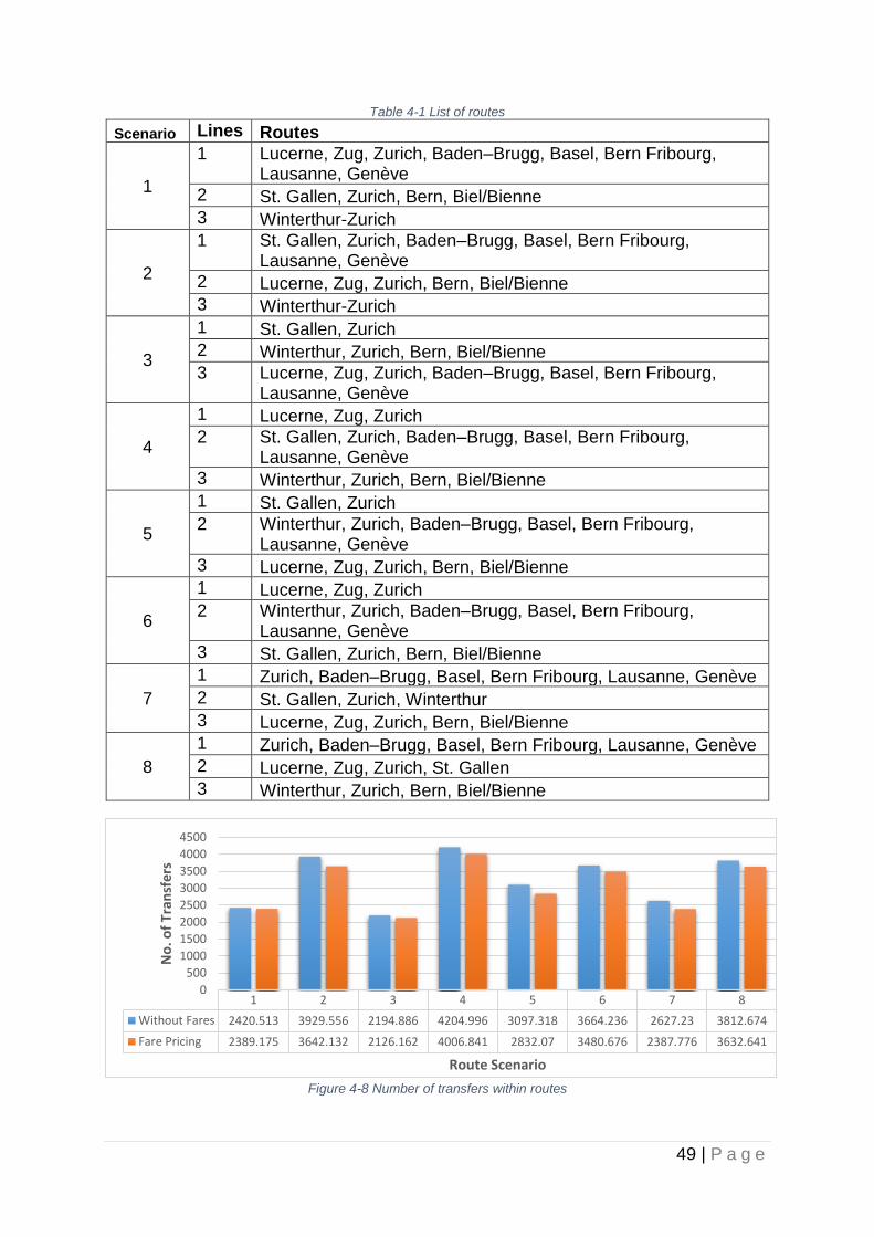
49 | P a g e
Table 4-1 List of routes
Scenario Lines Routes
1
1 Lucerne, Zug, Zurich, Baden–Brugg, Basel, Bern Fribourg, Lausanne, Genève
2 St. Gallen, Zurich, Bern, Biel/Bienne
3 Winterthur-Zurich
2
1 St. Gallen, Zurich, Baden–Brugg, Basel, Bern Fribourg, Lausanne, Genève
2 Lucerne, Zug, Zurich, Bern, Biel/Bienne
3 Winterthur-Zurich
3
1 St. Gallen, Zurich
2 Winterthur, Zurich, Bern, Biel/Bienne
3 Lucerne, Zug, Zurich, Baden–Brugg, Basel, Bern Fribourg, Lausanne, Genève
4
1 Lucerne, Zug, Zurich
2 St. Gallen, Zurich, Baden–Brugg, Basel, Bern Fribourg, Lausanne, Genève
3 Winterthur, Zurich, Bern, Biel/Bienne
5
1 St. Gallen, Zurich
2 Winterthur, Zurich, Baden–Brugg, Basel, Bern Fribourg, Lausanne, Genève
3 Lucerne, Zug, Zurich, Bern, Biel/Bienne
6
1 Lucerne, Zug, Zurich
2 Winterthur, Zurich, Baden–Brugg, Basel, Bern Fribourg, Lausanne, Genève
3 St. Gallen, Zurich, Bern, Biel/Bienne
7
1 Zurich, Baden–Brugg, Basel, Bern Fribourg, Lausanne, Genève
2 St. Gallen, Zurich, Winterthur
3 Lucerne, Zug, Zurich, Bern, Biel/Bienne
8
1 Zurich, Baden–Brugg, Basel, Bern Fribourg, Lausanne, Genève
2 Lucerne, Zug, Zurich, St. Gallen
3 Winterthur, Zurich, Bern, Biel/Bienne
Figure 4-8 Number of transfers within routes
1 2 3 4 5 6 7 8
Without Fares 2420.513 3929.556 2194.886 4204.996 3097.318 3664.236 2627.23 3812.674
Fare Pricing 2389.175 3642.132 2126.162 4006.841 2832.07 3480.676 2387.776 3632.641
0
500
1000
1500
2000
2500
3000
3500
4000
4500
No
. of
Tran
sfe
rs
Route Scenario

50 | P a g e
For scenario 3, along with the set of routes, the load profile has been plotted in Figure
4-9 and Figure 4-10. In both figures, it can be observed that the load is higher towards
major cities, namely Zurich and Bern. This observation is in-line with the input demand
of the morning peak hour. The morning peak hour demand showed a significant share
of commuting and educational trips towards major cities.
Due to the consideration of larger canton regions of Baden-Brugg (aggregation of 432
zones in Aargau) and Fribourg (canton 436 zones), the flow from these cantons turns
out to be very high. This leads to unrealistic frequency determination. Also, for the
network generation and route design, the whole public transport demand was
considered. This consideration was due to the limitation of demand estimation model
NPVM to estimate the mode-specific demand. Though while estimating demand, it
was observed that the Hyperloop Network generated 15%17 of the passenger-
kilometres. Given this argument, 15% of the maximum load is considered for the
frequency setting of each of the lines. The grey line (up direction) and the yellow line
(down direction) in Figure 4-9 and Figure 4-10 shows the service capacity of without
fare and ‘with fare’ scenario respectively.
The frequencies of each of the lines are shown in Figure 4-11 with a graphical
representation of the lines for both scenarios. These frequencies are rounded off to
the nearest 0.5. The figure shows the graphical representation of the generated
network with routes and frequency of respective lines. Based on the adapted approach
for frequency determination, it is quite evident that the line underutilised in terms of
frequency. This mainly because only one pair of stations are selected for line one. As
mentioned in the network generation section 4.1.1, the unexpected link is Zurich to St.
Gallen. Comparing with the developed Hyperloop network to Swissmetro network
(Figure 1.1), there was also a direct connection between Lucerne and Bern instead of
Bern to Zurich in Swissmetro. However, a higher demand between these two cities led
to the generation of a direct link in Hyperloop Network.
The following sub-section of the chapter shows the results generated from the
assignment model of NPVM. The number of vehicles required is part of the cost-
benefit analysis.
17 7345614 pass-km by Hyperloop of 905,019.40 pass-km total network. This can also depend upon the setting of frequency while estimating demand.

51 | P a g e
Figure 4-9 Load profile and service capacity of the lines: ‘without fare’ scenario
0
200
400
600
800
1000
1200
1400
St.Gallen - Zurich
No
of
Tri
ps
Stations
Line-1 Up
Down
0
500
1000
1500
2000
2500
3000
3500
4000
Winterthur - Zurich - Bern - Biel/Bienne
No
of
Tri
ps
Stations
Line-2 Up
Down
Up Direction Frequency Load
Down Direction Frequncy Load
0
2000
4000
6000
8000
10000
12000
Lucerne Zug Zurich Baden–Brugg Basel Bern Fribourg Lausanne Genève
No
of
Trip
s
Stations
Line-3Up
Down
Up Direction Frequency Load
Down Direction Frequncy Load

52 | P a g e
Figure 4-10 Load profile and service capacity of the lines: ‘with fare’ scenario
0
500
1000
1500
2000
2500
3000
3500
Winterthur - Zurich - Bern - Biel/Bienne
No
of
Tri
ps
Stations
Line-2 Up
Down
Up Direction Frequency Load
Down Direction Frequncy Load
0
200
400
600
800
1000
1200
1400
St.Gallen - Zurich
No
of
Tri
ps
Stations
Line-1 Up
Down
Up Direction Frequency Load
Down Direction Frequncy Load
0
2000
4000
6000
8000
10000
12000
Lucerne - Zug - Zurich - Baden–Brugg - Basel - Bern - Fribourg - Lausanne - Genève
No
of
Trip
s
Stations
Line-3 Up
Down
Up Direction Frequency Load
Down Direction Frequncy Load

53 | P a g e
Figure 4-11 Geographical map of Switzerland with Hyperloop Network including the routes and frequency

54 | P a g e
4.3 Assignment results The assignment is performed in the PTV Visum 16.01-04 version. The aforementioned
network of Hyperloop is formed with the public transport network of Switzerland for the
assignment. The assignment is performed for the peak hour (0700 hours to 0800
hours) of an average working day in the year 2040. These assignments are performed
with the new estimated demand for both scenarios. As mentioned in the assumptions
of the study, the demand matrix has been reduced to the border of Switzerland only.
The zones outside the border are not considered. This led to performing assignment
again for the base case as well.
The assignment results of the public transport network showed the mean perceived
journey time of 1h 32mins, 1h 42mins and 1h 46mins in base scenario, without fare
Hyperloop scenario and ‘with fare’ Hyperloop scenario respectively. However,
comparing them directly will not lead to actual evaluation. The increase in the mean
perceived journey time is due to weights of the travel time components especially
transfer penalty and transfer weight time (refer Table 3-5) in assignment procedure.
This leads to the passenger from inner regions to make a longer journey via Hyperloop
and will result in perceived journey time. However, this increase does not exceed than
the decrease in the mean journey time of car network. The actual comparison can be
made by only adding total travel times of car and PT network and multiplying with their
respective VoT. This is followed in travel time savings section of the CBA (refer section
4.4.5).
The comparison of pass-hours for both the networks is shown in Figure 4-12. The
overall mean journey time for both Hyperloop cases is higher since the demand is also
higher. The reduction in pass-hours of a car is observed to be 17.56% and 9.66% for
‘without fare’ and ‘with fare’ cases respectively. The passenger hours of public
transport are based on the ride time of the network. The ride time includes access time,
in-vehicle time, transfer wait time and egress time. The ride hours of public transport
are higher by 26.16% and 42.93% for the respective cases. However, the mean speed
of the public transport network is reduced by 1km/hr for both Hyperloop cases due to
addition of Hyperloop. This reduction is significant for the network of 30,530 routes and
17,689 stops.
Figure 4-12 Simulation results: Pass-hours
Base Case Scenario: Hyperloop without Fare Scenario: Hyperloop with Fare
Car 170960 140923 154439
PT 187632 268186 236710
0
0.5
1
1.5
2
2.5
3
Pas
s-H
ou
rsx
10
00
00

55 | P a g e
Figure 4-13 shows the comparison of the pass km for all scenarios with Car and PT
networks. ‘Without fare’, the scenario shows higher pass-km than the base scenario.
The Hyperloop scenario shows a 33% increase in the pass-km compared to the base
scenario. This will lead to a reduction in the operational cost of car network by 17.46%
(cost 0.16CHF/km)18. Similarly, ‘with fare’ scenario, 9.36% reduction is observed in car
operational cost. Here, it is also important to note that the pass-km for PT networks,
shown in Figure 4-13, is the ride distance. This includes the distance for access (the
distance within stop area) as well.
Figure 4-13 Simulation results: Pass-km
After performing assignments of the networks, the networks are assessed with cost-
benefit analysis in accordance with the Swiss norms. The following section explains
the same.
4.4 Cost-benefit analysis The CBA is performed in accordance with the Swiss CBA norms. The analysis
performed in this section is not complete in terms of consideration of types of cost and
benefits. However, this may be considered as the starting point for the discussion of
CBA for Hyperloop. The types of costs and benefits considered are limited to (i) initial
infrastructure cost, (ii) maintenance cost, (iii) operational cost (iv) travel time savings
(v) fare revenue.
Table 4-2 Summary of CBA
No Description without fare (BCHF) with fare (BCHF)
Costs Benefits Costs Benefits
4.4.1 Infrastructure Cost 51.59 51.52
4.4.2 Maintenance Cost 02.16 02.14
4.4.3 Replacement Cost 02.92 02.84
4.4.4 Operational Cost 06.89 06.82
4.4.5 Travel Time Savings 33.57 03.89
4.4.6 Fare Revenue 72.95 97.46
Total 61.98 106.52 61.78 101.35
B/C ratio 1.69 1.61
18 (ARE, 2014)
Base CaseScenario: Hyperloop without
FareScenario: Hyperloop with Fare
Car 13323214 10995946 12048670
PT 9430913 12575613 11334208
0
5
10
15
Pas
s-km
Mill
ion
s

56 | P a g e
It is important to mention that the analysis does not consider an increase in the
operational cost of the existing public transport network or a decrease in the operating
cost of cars. Since the demand for the car network is reduced, the maintenance cost
of the same will be reduced as well. However, this is not considered in the analysis.
The analysis period is performed for 50 years, assuming the infrastructure construction
duration would be five years (2036-2040). The operations will start in the year 2040.
The benefits from 2040 to the next 49 year i.e. up to the year 2089. Table 4-2 shows a
summary of the costs and benefits. The costs and benefits are in the net present value
of the year 2040 i.e. discounted with a 2% discount rate to the reference year. The B/C
ratio turns out to be 1.69 for the without fare scenario and 1.61 for the ‘with fare’
scenario. These numbers show significant gains over costs incurred. However, it is
important to mention that these numbers are not part of the complete analysis and an
exhaustive number of assumptions are involved in this analysis, which can change the
output or interpretation largely.
Figure 4-14 and Figure 4-15 show the cashflow of discounted benefits over the analysis
period. Both the figure shows a drop in the benefits in the year 2059 and in the year
2079 due to replacement cost of vehicles, propulsion system and ventilation. Similarly,
the drop in the benefits in the year 2064 is due to the replacement of the solar panels.
The internal rate of return (IRR) turns out to be 3.30% and 2.90% for ‘without fare’ and
‘with fare’ scenario respectively. The discounted payback period is 24 years and 25
years for the respective scenario. The scenario ‘with fare’ shows comparatively better
results than without fare scenario. However, the actual willingness to pay for the user
is still debatable. This is discussed in the discussion section of the report.
The costs and benefits mentioned in Table 4-2 are explained in more detail below:
4.4.1 Infrastructure cost
The infrastructure costs per unit are described in detail in chapter 3 of the document.
Also, the output of the network generation algorithm gives the cost of the network for
construction. However, the cost considered for the network generation algorithm is
average annual cost and after the route design and frequency setting, the unused links
need to be removed as well. This leads to a re-calculation of the infrastructure cost.
Figure 4-11 shows the network after the removal of unused links. This network has a
total length of 1026.418 km.
As mentioned in section 3.2.1, the total number of stations is 12. However, from the
network structure, Bern and Zurich are hubs of the network i.e. being junctions of three
or more lines. Thus, the cost of these stations is multiplied by a factor of 1.5 more than
the estimated per station cost. For the rest of the stations, the estimated cost has been
assumed.
This leads to a total cost of 51.32BCHF. This does not include the cost of vehicles.
This will also remain the same for both cases.
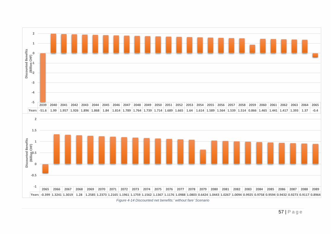
57 | P a g e
Figure 4-14 Discounted net benefits:’ without fare’ Scenario
2039 2040 2041 2042 2043 2044 2045 2046 2047 2048 2049 2050 2051 2052 2053 2054 2055 2056 2057 2058 2059 2060 2061 2062 2063 2064 2065
Years -51.6 1.99 1.957 1.926 1.896 1.868 1.84 1.814 1.789 1.764 1.739 1.714 1.689 1.665 1.64 1.614 1.589 1.564 1.539 1.514 0.866 1.465 1.441 1.417 1.393 1.37 -0.4
-5
-4
-3
-2
-1
0
1
2
Dis
cou
nte
d B
en
efi
ts(B
illio
n C
HF)
2065 2066 2067 2068 2069 2070 2071 2072 2073 2074 2075 2076 2077 2078 2079 2080 2081 2082 2083 2084 2085 2086 2087 2088 2089
Years -0.399 1.3241 1.3019 1.28 1.2585 1.2373 1.2165 1.1961 1.1759 1.1562 1.1367 1.1176 1.0988 1.0803 0.6424 1.0443 1.0267 1.0094 0.9925 0.9758 0.9594 0.9432 0.9273 0.9117 0.8964
-1
-0.5
0
0.5
1
1.5
2
Dis
cou
nte
d B
en
efi
ts(B
illio
n C
HF)

58 | P a g e
Figure 4-15 Discounted Net Benefits: ‘with fare’ Scenario
2039 2040 2041 2042 2043 2044 2045 2046 2047 2048 2049 2050 2051 2052 2053 2054 2055 2056 2057 2058 2059 2060 2061 2062 2063 2064 2065
Years -51.5 3.595 3.536 3.479 3.424 3.37 3.318 3.267 3.216 3.167 3.118 3.069 3.021 2.973 2.925 2.877 2.83 2.784 2.737 2.692 2.068 2.602 2.559 2.515 2.473 2.431 0.645
-5
-4
-3
-2
-1
0
1
2
3
4
Dis
cou
nte
d B
en
efi
ts(B
illio
n C
HF)
2065 2066 2067 2068 2069 2070 2071 2072 2073 2074 2075 2076 2077 2078 2079 2080 2081 2082 2083 2084 2085 2086 2087 2088 2089
Years 0.645 2.35 2.31 2.271 2.232 2.195 2.157 2.121 2.085 2.05 2.015 1.981 1.947 1.915 1.493 1.85 1.819 1.788 1.758 1.728 1.699 1.67 1.642 1.614 0.986
-1
-0.5
0
0.5
1
1.5
2
2.5
3
3.5
4
Dis
cou
nte
d B
en
efi
ts(B
illio
n C
HF)

59 | P a g e
4.4.1.1 Vehicle Cost
The number of vehicles required is calculated based on the cycle time of each line and
headway per direction. The headways are calculated based on the frequency shown
in Figure 4-11. Table 4-3 shows the number of vehicles required for each line along
with cycle time and headway. 20 minutes19 is added in the cycle time as the turnaround
time. One extra vehicle is also added for each line in each direction, for the breakdown
and other purposes. The vehicles are rounded off on the higher side. Line-3 shows a
higher number of vehicles required since the cycle time is high, and the headway is
very low.
Table 4-3 Number of vehicles required
Line Cycle Time ‘without fare’ Scenario ‘with fare’ Scenario
Headway No. of
Vehicles
Headway Number of
Vehicles Up Down Up Down
1 14 mins 45s 15 mins 30 mins 3 20 mins 30 mins 3
2 26mins 5s 5 mins 30s 6 mins 11 6min 40s 8 mins 8
3 50 mins 55s 5 mins 2 mins 40 6min 20s 2 mins 20s 28
This results in a total number of vehicles required to be 60 and 45 for ‘without fare’
and ‘with fare’ scenario. Considering the 4.5 MCHF per vehicle cost, this will lead to
270MCHF and 202.5MCHF in the respective cases.
This leads to a total initial infrastructure investment cost of 51.59BCHF and
51.52BCHF for ‘without fare’ and ‘with fare’ cases respectively. This includes the cost
of land and design planning.
4.4.2 Maintenance cost
After the initial infrastructure cost, the maintenance cost is considered the same as is
explained in section 3.1.2. This consideration is taken on the basis of the average
annual cost. Per year maintenance cost for track part is 55.62MCHF and 10.06MCHF
for the station part. The cost for vehicle maintenance annually will be 1.62MCHF for
‘without fare’ scenario and 1.22MCHF ‘with fare’ scenario. This leads to a total of 2.16
BCHF and 2.14 MCHF of maintenance cost for the ‘without fare’ and ‘with fare’
scenario respectively over the analysis period.
4.4.3 Replacement cost
During the analysis period, propulsion system, vacuum pumps and vehicles will be
required to be replaced twice, while the solar panels will be required to replace once20.
This will lead to the addition of 2625.11MCHF for infrastructure-related elements; and
for vehicles 286.853MCHF and 215.140MCH for ‘without fare’ and ‘with fare’
scenarios, respectively. This results in a total of 2911.96 MCHF and 2840.25MCHF of
the replacement cost.
4.4.4 Operational cost
The operational cost has two considerations in terms of Hyperloop infrastructure,
namely the stations and the vehicles. The operational cost for 12 stations would be
19 10 minutes on each end for cleaning and break for the staff (layover/ turn around). 20 Age as per the table Table 3-3

60 | P a g e
206.92 MCHF annually. This will lead to 6.632 BCHF over the analysis period. The
vehicle operational cost has been divided into two parts i.e. staff cost and energy cost.
The staff cost is directly proportional to a number of vehicles, while the energy cost is
proportional to travelled seat-km. The staff cost will be 7.11BCHF and 5.33BCHF
annually for the ‘without fare’ and ‘with fare’ scenario respectively. This is calculated
based on the number of vehicles mentioned in the sub-section4.4.1.1 and per vehicle
staff cost mentioned in Table 3-3.
To calculate the energy cost, seat-km operated is required. Based on the frequency
mentioned in Figure 4-11, the peak hour seat-km will be 16,954.786 seat-km and
13,677.736 seat-km for ‘without fare’ and ‘with fare’ case respectively. The peak hour
model consists of 10% of the public transport daily demand (ARE, 2016). Assuming
the same proportion for the Hyperloop seat-km, this will turn into 42.56Mseat-km and
34.33Mseat-km annually for ‘without fare’ and ‘with fare’ respectively. Based on the
operational cost mentioned in Table 3-3, the total vehicle operational cost over the
analysis period will be 16.55MCHF and 13.35MCHF for ‘without fare’ and ‘with fare’
case respectively.
Thus, the total operational cost over the analysis period turns out to be 6.88BCHF and
6.82BCHF for ‘without fare’ and ‘with fare’ cases respectively. This also considers the
population growth of 0.26% every year.
4.4.5 Travel time savings
Figure 4-16 shows the travel time results of peak assignment in the form of costs.
From the figure, it can be observed that the travel times components of public transport
show increase in the Hyperloop cases. This is because of the higher demand than the
base case. In a similar way, the car networks show a reduction in total travel time,
since lesser demand has reduced the congestion on the roads and also the demand
is reduced as well compared to the base case.
The values of ‘without fare’ and ‘with fare’ cases are subtracted, from the base case
from Figure 4-16 to calculate the travel time savings. These values are for peak hour.
Therefore, they are converted to daily and annual numbers. As mentioned before, the
car network captures 7.2% demand in peak hour of the daily demand, while PT
network 10.0% (ARE, 2014). These ratios are applied to convert the values in daily
travel time savings. Subsequently, to convert into annual values, 251 working days
are considered as mentioned before.
Once the annual travel time savings are projected, the unit cost of the respective travel
time component from section 3.2.2.3 is multiplied to convert the travel time savings in
monetary values. This results in annual travel time savings of 992.49MCHF and
114.98MCHF for ‘without fare’ case and ‘with fare’ case respectively.

61 | P a g e
Figure 4-16 Travel time cost for peak hour in 2040
These annual values are compounded with the population growth factor of 0.26%21
yearly up to 2089. This leads to total travel time savings over the analysis period
3.89BCHF and 33.57 BCHF for ‘without fare’ and ‘with fare’ cases respectively.
The travel time savings in ‘with fare’ case is significantly lower, compared to without
fare case. This is mainly because of Access time. With fair case shows, 2.5 access
time savings compared to without fare case, this has led to the higher difference in the
cost value of access time savings as well because of the higher unit value of access
time savings.
4.4.6 Fare revenue
The revenue is calculated based on the pass-km for Hyperloop. NPVM considers the
cost of 0.20CHF/km (2010 rates) for PT. For without fare case, the same i.e.
0.36CHF/km (2040 rates) is considered, while for the fare case 0.50CHF/km (2040
rates) is considered. The pass-km can be directly extracted from the Visum
assignment results. The assignment shows 2,386,870 pass-km and 2,296,132 pass-
km for the Hyperloop system for ‘without fare’ and ‘with fare’ cases respectively.
Similar to the previous subsection these values are projected for annual values and
aforementioned costs are applied. This leads to revenue of 2,156.78 MCHF and
2,881.65 MCHF annually. It can be noted that these numbers are significantly higher
than the annual total operational cost.
Similar to travel time savings, these numbers are discounted for the analysis period
with 2% and population growth rate of 0.26% is also applied to compound annually.
This results in 72.95BCHF and 97.46BCHF revenue for ‘without fare’ and ‘with fare’
cases respectively. The value of ‘with fare’ case is higher since the value of fare itself
is significantly higher in the latter case. However, here it is required to mention that all
the public transport modes observed an increase in the pass-km except long-distance
21https://www.bfs.admin.ch/bfs/en/home/statistics/population/population-projections/national-projections.html
Car Travel Time In Vehicle TimeTransfer Waiting
TimeNumber of
Transfers (No)Access Time
Base Case 266451 148130 16440 187178 48785
Fare Case 239521 172285 36728 319440 54608
HL Case 213970 195832 40842 360677 61218
0
5
10
15
20
25
30
35
40Tr
ave
l Tim
e C
ost
in H
ou
rsx
10
00
0
Travel Time Component

62 | P a g e
trains. The long haul-double decker trains observed the loss of 33.49% and 38.52%
loss of pass-km in ‘without fare’ and ‘with fare’ cases respectively.
After describing the CBA, the following section explains the results of the sensitivity
analysis.
4.5 Sensitivity analysis The section explains the sensitivity analysis performed for the network design process.
This analysis is performed based on the Cost, VoT and Discount rate criteria. These
criteria are selected based on the Swiss CBA norms. However, the norms also suggest
demand as a criterion, but a due limitation of actual demand estimation, this criterion
is not considered. To some extent, the scenario of ‘with fare’ also gives an indication
of the network changes due to change in the demand. The study evaluates each phase
of the network design for the sensitivity i.e. network generation, route design and CBA
in ‘without fare’ scenario.
Considering the above-mentioned criteria for sensitivity, the discount rate is effective
only in the cost-benefit analysis part, while the changes in costs and VoT are effective
in all the phases. The cost considers all the cost from the supply side i.e. infrastructure,
maintenance & operational cost. Given that, reduction in cost improves the B/C ratio
only. This is less interesting compared to an increase in the cost. Therefore, an
increase in the cost is only considered for the analysis. For the VoT, increase and
decrease, both are considered for all the components of the travel time as per the
Swiss CBA norms (Association Suisse des Professionnels, 2006).
As Table 4-4 shows, for the cost, four criteria are selected based on increase side at
the 10% interval each, while for the VoT four criteria, with 10% of interval on each
increase and decrease sides. For the discount rate, the norms suggest performing
analysis with the value above 3%. This leads 50% minimum increase in the discount
rate. These sensitivities are explained network design phase-wise in detail in the
following subsections.
Similar to a traditional swiss public transit network, without fare scenario is considered
for the sensitivity analysis.
Table 4-4 Sensitivity criteria
Criteria Change in Value
Cost - +10% +20% +30% +40%
VoT -20% -10% - +10% +20%
Discount Rate - +50% +60% +70% +80%
4.5.1 Sensitivity in network generation
From the results, it is realised that both the approaches generate the same networks
as far as the minimum spanning tree network has a B/C ratio above one. With each of
the cost increase of 10%, one bi-directional link is reduced from the network. This
leads to networks with 15(Figure 4-17), 14(Figure 4-18), 13(Figure 4-19), 12(Figure
4-20) number of links 10% higher cost. With a 50% higher cost case both the algorithm
develops a different solution. However, that case is not considered as a part of this
analysis. This will develop a lot of routes and will lead to higher operational cost for
the link deletion algorithm.

63 | P a g e
With 10% variation in the VoT, the networks do not show any variations in terms of
network structure and number of links. However, with 20% variation in the VoT the
network shows a difference in the structure. The network with 20% reduction in the
VoT shows 15 number of links (Figure 4-18) (same network structure as 10% increase
in the cost), while 17 number of links in case of 20% increase in the VoT (Figure 4-21).
The increase in the VoT leads to increased benefits of the network and higher benefits
would allow more feasible links. In all the cases, the link swapping and link deletion
algorithm make provides a solution with a B/C ratio above 1.
After network generation, the following subsection explains route design and
frequency setting.
Figure 4-17 Network with cost +10%
Figure 4-18 Network with cost +20% and VoT -20%

64 | P a g e
Figure 4-19 Network with cost +30%
Figure 4-20 Network with Cost 40%
Figure 4-21 Network with VoT +20%

65 | P a g e
4.5.2 Sensitivity in routes
The change in the network structure also leads to a different set of routes. Considering
the adapted approach for the route design, the networks do not show much variation.
The routes generated can be categorized into three different types. This list is shown
in Table 4-5 are finalized routes for different network structure with calculated
frequency and number of vehicles required based on the cycle time of each line. These
routes, as per the categories and frequencies are shown in the table.
Table 4-5 Sensitivity in routes
Type Line Stations Frequency No of Vehicles Up Down
1
1 St. Gallen, Zurich 3 2
60 2 Winterthur, Zurich, Bern, Biel/Bienne 11 10
3 Lucerne, Zug, Zurich, Baden–Brugg, Basel, Bern Fribourg, Lausanne, Genève
12 32
2
1 Lucerne, Zurich 2 2
58 2 Zug, Zurich, Bern, Biel/Bienne 9 8
3 St. Gallen, Winterthur, Zurich, Baden–Brugg, Basel, Bern Fribourg, Lausanne, Genève
14 28
3
1 Lucerne, Zug, Zurich, Bern, Biel/Bienne 13 12
51 2 St. Gallen, Winterthur, Zurich, Baden–
Brugg, Basel, Bern Fribourg, Lausanne, Genève
17 33
The type 1 and 2 generated 8 different scenarios with routes, while type three
developed 4 different scenarios of the routes. Type 1 routes are the same as the routes
developed for the actual case. Type 2 routes are generated because Zug and Lucerne
are not connected, while Winterthur and St. Gallen are connected. Type 3 routes have
only two lines. This is because of fewer links in the network. This also leads to a smaller
number of transfers overall Hyperloop networkwide. These route types related to
different network cases are shown in Table 4-6. To define the frequency and number
of vehicles required, a similar approach is adopted as described in the previous
section.
After identifying routes, frequencies and required number of vehicles, similar to
previous section assignment are performed with all the types of routes with an existing
network. The results of the assignment are directly showed with the B/C ratio.
Table 4-6 Route types with networks generated (con: Table 4-5)
1 2 3
1
Cost
+10% X
2 +20% X
3 +30% X
4 +40% X
5
VoT
-20% X
6 -10% X
7 +10% X
8 +20% X

66 | P a g e
4.5.3 Sensitivity in cost-benefit analysis
After generating routes and frequencies, the B/C ratio needs to be re-calculated. In this
stage of the analysis, the discount rate sensitivity case is also included.
Figure 4-22 B/C ratio vs Change in sensitivity criteria
Figure 4-22 shows the results from the sensitivity analysis. From the figure, it can be
overserved that for all the cases, the B/C ratio remains above one. This is mainly
because all the networks generated have initial B/C ratio above 1.
The discount rate shows a linear relationship with the B/C ratio. With every increase of
10% in the discount rate 0.04 reduction is noted in the B/C ratio. The minimum value
of the B/C ratio turns out to be 1.31 in the case of discount rate with 80%. The purpose
of the sensitivity in the discount rate is to capture the economical variations especially
inflation. However, it should be noted that in the current analysis, the prices projected
for the 2040 year are not changed. The values after the year 2040 up to analysis period
only affected.
For the cost, the small increase led to a higher reduction in the B/C ratio compared to
the discount rate. Figure 4-22 shows a sharp decrease in the B/C ratio at 20% increase
in the cost. This is because of changes in the routes of the networks. With a 40%
increase in the cost less reduction in B/C ratio is observed since this network is covered
with a smaller number of routes. Also, the travel time savings increases with a
reduction in a number of transfers.
Changes in VoT with 10% variation shows an almost linear relationship with the B/C
ratio, as no changes in the networks are observed. With both extreme cases of VoT,
the B/C ratio shows large variations. With a 20% reduction in VoT the B/C ratio drops
to 1.30 and with 20% increase it reaches to 1.93.
To summarize, the discount rate shows a linear relationship with the B/C ratio, while
cost and VoT shows linear until changes in routes. The change in the routes shows
significant changes in the B/C ratio since it changes travel time savings, the number of
vehicles required, and operational costs.
-20% -10% 0% +10% +20% +30% +40% +50% +60% +70% +80%
Cost 1.69 1.57 1.40 1.32 1.30
VoT 1.30 1.63 1.69 1.74 1.93
Discount Rate 1.43 1.39 1.35 1.31
0.8
1
1.2
1.4
1.6
1.8
2
B/C
rat
io
Change in the Value

67 | P a g e
5 Conclusion & limitations
The current chapter of the document summarizes the key findings, limitations and
future research. The key findings are described by answering the sub-research
questions leading to answering the main research question. The subsequent section
describes the limitations of the study and at the end, perspective for the future research
is given.
5.1 Key findings As mentioned before, the section describes the findings by answering the sub-research
questions and the main research question. These findings are explained in a
generalized manner as well as at the case-specific level. The case-specific answers
may change according to the conditions of the respective case. The sub-research
questions one and two focus on generalized findings, while sub-research questions
three, four, five and six describe case-specific findings as well.
1. What are the inputs required for the network design of a Hyperloop
system?
For the approaches of network design adopted in the current study, the inputs are
(i) unit costs of infrastructure, operations and user; (ii) the demand for the network
with existing travel times and (iii) the set of nodes (stations). These inputs are
prepared either from the secondary data collected or from the available literature.
It is observed that the network structure is highly correlated with the given inputs,
especially costs and demand. The major assumption pertaining to the input of the
demand and nodes is that they are considered fixed throughout the designing
process. The total costs of the network vary with the network structure. However,
these total costs do not capture the additional expenses incurred due to a change
in the alignment of lines (such as curvature) and other critical geographical factors.
The total demand of all the networks remains fixed throughout the design process.
This is because induced demand is not considered in this research. The network
structure is highly correlated with the input unit infrastructure & user cost (VoT), and
demand. Rather than considering the speed of the mode (Hyperloop), seating
capacity of a vehicle, and headway as design parameters, they can also be
considered as variable inputs for the developed design process. This allows room
for variations according to the design requirements of a study.
2. What are the methods to design/optimise transit networks such as
Hyperloop?
From the literature, mainly four types of designing and optimising methods are
identified. These methods are namely Conventional, Mathematical Programming,
Heuristics and Meta-Heuristics. These methods have their own advantages and
shortcomings mainly in-terms of computational time, quality of results and
complexity of implementation. After comparing these characteristics, the current
research is performed based on heuristic methods from the author’s perspective.
The application of the methods can largely be categorised in two phases i.e.
defining network structures (network generation) and designing routes.

68 | P a g e
The methods adopted for network generation algorithm namely link swapping and
link deletion, are modified from the method of Bell et al. (2019). Both the methods
generate the same outputs, provided the minimum spanning tree network has a
B/C ratio greater than one. On the contrary, when the minimum spanning tree
network has a B/C ratio less than one, both approaches generate different outputs.
In the former case which is relevant to the current study, both the algorithm
develops an output of heuristic nature. They identify the feasible set of links to
design the routes.
The method for route design develops a set of candidate routes and subsequently
looks for a feasible solution within the candidate set. The method is based on the
algorithm developed by Mandl C. E. (1980). This output is also heuristic of its nature
since optimisation takes place only within the candidate set of routes. The
candidate set of routes is developed by identifying the longest shortest path on the
feasible network. Subsequently, these routes are optimised based on the number
of transfers i.e. user cost.
3. What is the feasible set of links in a Hyperloop network with respect to
benefit to cost (B/C) ratio?
This research question is answered via the output of the network generation
algorithms. The output of each algorithm generates a set of links. These sets of
links are generated by making sure that the B/C ratio of the network remains above
one. However, here the B/C ratio consists of infrastructure cost and travel time
savings (in-vehicle time) only. The set of links generated by the algorithms are such
that any other non-chosen links will not have higher flow than selected links if they
are added to the network. However, the generated set of links may be redundant
in the network. This means that the B/C ratio is not maximum for the network for
the considered costs.
For the current case of Switzerland, two scenarios are analysed: (i) ‘without fare’
scenario i.e. Hyperloop being part of the national subscription along with with rest
of the PT network (ii)’with fare’ scenario i.e. a separate fare pricing system for the
Hyperloop service. For the chosen 12 input nodes, 16 feasible bi-directional links
for ‘without fare scenario’ and 15 feasible bi-directional links for ‘with fare scenario’
are identified. The ‘with fare scenario’ has less a link relatively since the demand is
reduced.
4. Which is the optimal set of routes for the Hyperloop network generated in
the previous sub-research question? What are the frequencies and
number of vehicles required for the respective lines?
On the generated network from the previous sub-research question, the lines are
identified for a set of routes for both the cases. These lines are selected based on
the longest shortest path of the networks generated. Once every node is covered
by at least one line, no further lines are identified. Once the lines are defined,
optimisation takes place based on the number of transfers. To optimise the number
of transfers, different combinations of lines are generated by swapping the portions
of the lines from the transfer node. These combinations can be in total 2n, where n
is the number of lines identified. The algorithm partially lowers the cost of operation
69 | P a g e
by selecting a minimum number of lines. Subsequently, it optimises the user cost
based on the number of transfers.
In the current swiss case, three lines were identified in both scenarios – ‘without
fare’ and ‘with fare’. These three lines led to the generation of eight different
combinations to optimise the set of routes based on the number of transfers. Since
both the networks had a similar structure of the network, they resulted in the same
set of routes.
The frequencies are defined based on the maximum load of a link. This approach
of defining frequencies might have generated higher empty pass-km as frequencies
are not optimised. Out of both the scenarios, the maximum and minimum
determined frequency of 32 and 2 is found per hour. The lines with a minimum
frequency of two depict that it is underutilisation. Based on the frequencies and
cycle times of each line the number of vehicles required is identified. This turns out
to be 60 nos. and 45 nos. for ‘without fare’ and ‘with fare’ case respectively.
5. What is the B/C ratio of the Hyperloop network generated in previous sub-
research question?
This sub-research question is difficult to answer in a generalised manner as B/C
ratios are always specific to the case and scenario under consideration. The results
from the analysis show the B/C ratio of 1.69 and 1.61 for the ‘without fare’ and ‘with
fare’ cases respectively. Though the fare revenue increases for the ’with fare’ case,
the travel time savings and demand both decreased significantly for the same. For
the ‘without fare’ scenario, the discounted internal rate of return turns out to be
3.24% with the discounted payback period of 24 years. For the ‘with fare’ scenario
the discounted internal rate of return turns out to be 2.90% with the discounted
payback period of 25 years. However, in terms of economic B/C ratio i.e.
considering only monetary parameters (without travel time savings), these ratios
turn out to be 1.15 and 1.53 for the ‘without fare’ and ‘with fare’ scenario
respectively. In this situation, though the demand is lower in the ‘with fare scenario’,
the revenue generated from the fare is significantly higher because of a higher
value of fare per km (the fare for the Hyperloop is 40% higher than base fare of the
public transport per km) itself.
6. To what extent is the B/C ratio of the Hyperloop network sensitive to its
design inputs?
The sensitivity analysis performed on the Hyperloop network shows expected
results. Mainly three criteria are considered this for analysis, namely the discount
rate, VoT and costs. The discount rate shows a linear relation with the B/C ratio.
The increase in the discount rate leads to a decrease in the B/C ratio.
The network generation algorithm generates more links than required to cover the
routes for the case. Because of this, two observations are made – (i) with the
change in the network structure, different set of routes are generated (ii) with the
change in network structure, the routes remain the same.
The cost and VoT also show a linear relation with the B/C ratio. The cost is inversely
proportional to the B/C ratio, while VoT is directly proportional to the B/C ratio. It is

70 | P a g e
observed that the gradient of the B/C vs Cost and B/C ratio vs VoT changes as
routes are changed in the network.
In the current case of Switzerland, the sensitivity analysis is performed on ‘without
fare’ scenario. The analysis of the discount rate between the interval of +50% to
+80% shows ratio linear decrease in the B/C ratio from 1.43 to 1.31. In the B/C ratio
vs cost curve, the B/C ratio ranges from 1.69 to 1.30 with the cost of +0% to +40%.
Similarly, the B/C ratio changes from 1.30 to 1.93 for the interval of -20% to +20%
in VoT. All of the three criteria are analysed with every 10% interval.
Thus, answering the sub-research question leads to the answer to the main research
question. The main research question is answered by explaining a generalised solution
followed by key findings realised from the case of Switzerland.
“How can a Hyperloop network be designed based upon the determinants of the
cost-benefit analysis?”
The determinants of the cost and benefit analysis consist of (i) infrastructure cost, (ii)
maintenance cost, (iii) operational cost, (iv) replacement cost (v) travel time savings
and (vi) fare revenue. It is difficult to incorporate all the determinants in each phase of
the network design process. This is because the method adopted in this study is
sequential. In this case, the network generation phase includes travel time savings (in-
vehicle time savings) and infrastructure cost. In the route design phase, the routes are
generated in a way that a minimum number of lines are required to cover the network.
This minimises the operational cost to some extent. Subsequently, the number of
transfers is minimised on the candidate set of lines, which in turn leads to minimisation
of the user cost. On the other hand, the frequency setting does not involve optimisation.
This may lead to a higher number of vehicles required. The overall procedure is aimed
at generating a network that has a B/C ratio above one. In case, it is unable to do so,
a maximum possible B/C ratio less than one is attained.
The aforementioned procedure can give an indication of how determinants of costs
and benefits can be involved in the network design process. Indeed, the considered
costs and benefits for defining the network structure and routes are not complete.
However, these can be improved by adding more costs and benefits parameters
further, especially in terms of externalities like environment emissions, noise, accident
cost and many more. This will also improve the design towards the viability of the
networks.
For the case of Switzerland, two scenarios are analysed: (i) ‘without fare’ scenario i.e.
Hyperloop being part of the national subscription along with with rest of the PT network
(ii)’with fare’ scenario i.e. a separate fare pricing system for the Hyperloop service.
With beta parameters of the existing public transport network, the Hyperloop could
make the modal-shift of 11% and 6.5% of the car demand in ‘without fare’ and ‘with
fare case’ respectively. For the demand estimated, the generated networks and
designed route could reduce the total travel time of the PT network significantly. This
led to a B/C ratio of 1.69 and 1.61 for the ‘without fare’ and ‘with fare’ cases
respectively. The higher B/C ratio of without fare scenario is because it could attract
more demand from the car network. However, here significant loss of pass-km is also
found in the long-haul trains. The performed CBA included determinant costs and

71 | P a g e
benefit only. For both the scenarios, it is found that the annual operational cost is
covered by annual fare revenue for all the years. This is an important observation for
a public transport system.
5.2 Limitations The current section of the document discusses the limitation of the study in each phase
and recommends further improvements for the same. The section first describes the
methodological limitations, followed by input related limitations and lastly, limitations
due to the assumptions made during analysis. The methodological limitations discuss
the global assumptions, while the analysis limitations discuss the case-specific
assumptions. The section of input limitations is discussed by comparing global and
case-specific assumptions.
5.2.1 Methodological limitations
The study adopted the fixed demand approach since the case study has a separate
interface for network simulations and for the decision model of the demand estimation.
This is mainly to reduce the overall computational time and to study the characteristics
of the networks individually. The simulated networks in the case study are also divided
further divided into car and PT network by NPVM. Combining these elements i.e.
making demand iterative along with the changes in the network could give better
results for the overall network design. This could be further extended by making routes
iterative to network generation. The current sequential approach of route design also
generated a limited number of candidate routes. This would turn results heuristic by
nature. Combining the interface of network generation route design and simulation
would improve the quality of the results.
The link swapping algorithm selects maximum direct demand nodes while adding links.
On the removal side, both the algorithms remove links based on the minimum flows.
These criteria were adopted for reducing the complexity of the algorithms. The addition
and removal criteria can be further improved by considering the B/C ratio as an adding
and removing criteria as well. Adapting these criteria along with the iterative demand
could extend the network generation algorithm itself towards optimizing. This would
also solve the issue of generating mono-centric networks mentioned in section 4.1.2.
The B/C ratio for the network generation could only consider the travel time savings on
the basis of direct travel. This is mainly due to limited literature available for the other
benefits and cost elements. For example. internalities like environment emissions,
accident cost, noise, etc. Adding these components in the objective function itself could
improve the design.
Given the size of the study area, the optimization on networks is performed considering
the constraint of the connected network. This was also considered due to higher
operational cost of stations. However, the possibility of disconnected networks still
needs to be explored.
In the route design phase, the routes are optimized based on the number of transfers
i.e. user cost. It could not capture the cost of the vehicles. However, considering the
longest shortest path for the candidate routes, partially lower the operational cost
(including vehicles required), but do not optimize. The frequencies are determined

72 | P a g e
based on the maximum load on the link in peak hour. This could have overestimated
the vehicles required and resulted in a higher cost for the same.
5.2.2 Input limitations
The major limitations of the study are due to the inputs. This includes mainly cost-
related and demand related limitations.
The demand estimation for public transport network including Hyperloop is performed
considering the same beta parameters as an existing public transport network. This is
mainly due to the unavailability of the literature or data to estimate the values. This
needs to improve by estimating the new values for beta parameters. In principle,
adding Hyperloop to the public transport network will improve the attractiveness and
VoT of the overall network. A detailed study needs to be performed for estimating these
beta parameters. Similarly, the variable values for parking time and parking cost for
the car network was not available. This increased the error in demand estimation. The
demand estimation does not consider capacity constraints. However, this is more
related to simulation and analysis. This will be discussed in further sub-section of
simulation limitations.
NPVM considers the same fare for all the public transport mode. This is because all
the public transport operators within Switzerland are obliged to provide service under
this national subscription of General Abonnement. This makes it difficult to estimate
the demand based on the different fare pricing for Hyperloop. To overcome this issue,
the current study translates overhead fare price of Hyperloop into in-vehicle time.
However, this conversion will not do justice to actual effects on demand due to different
weights of variables.
The assumption that Hyperloop characteristics are similar to those of conventional
public transport also needs to be verified. However, for the current research, some
characteristics of the Hyperloop are based on the conventional scheduled services.
The assumptions of speeds are based on the musk studies and limitation of the
simulating software Visum. The Musk study estimates the speed of 1,220km/hr with
1G acceleration. These assumptions are reduced due to 500 km/hr & 1,000km/hr and
0.5G based on the distances (30km link length criteria) to make them more realistic
values.
From the cost side, very limited literature is available to estimate the cost. However,
estimation from these studies also varies in a large range. This is mainly due to
uncertainty about the viability of materials to be used for the infrastructure. For e.g.
study from Transpod performed cost estimation by assuming steel material for tubes,
while musk estimation follows concrete for the same. The issue of cost is also relevant
to vehicles because of different sizes being predicted for the Hyperloop. The other
major cost consideration is related to operational cost. Only one study is performed
evaluating the operational cost of Hyperloop, in which, the cost estimates are specific
to the assumption related to specifications of the vehicles and infrastructure made in
the study. Projecting the same estimates for the current study could have deviated the
results. Since the operational cost has a large impact on the profitability of the projects,
this needs to be improved primarily. This will also give the base for the fare pricing.

73 | P a g e
The cost from the countries is converted based on the purchasing power parity. This
approach does not capture the actual market values. However, this approach also
needs to consider the things which can be developed locally or need to be imported.
The assumption of access time for the Hyperloop stations is also optimistic in the
current study. It is assumed that the access time for Hyperloop station will be similar
to the main railway stations. This is mainly due to the assumption of mounting
Hyperloop stations on existing railway stations and using Hyperloop for a daily
commute. However, operating services at high speed of 1000km/hr might need some
consideration of safety. This can result in increased access time. Mounting Hyperloop
stations on existing stations would lead to questions of both space and design. The
current study assumes the cost for land and design based on the percentage value of
the investment specific to the infrastructural element. The assumption is also valid due
to unavailability of such preliminary designs. Transpod study has given reliable
assumptions for the Tube part of the infrastructure with preliminary designs. Similarly,
other major elements can be investigated, which will lead to better estimates.
The other major missing element from the cost perspective is Switches on the stations.
There is no description in the literature about switches except the Delft Hyperloop
Study. The cost for the switches in the study is significantly over-estimated. This also
needs a thorough investigation. Shifting from one tube to another will require switches.
Apart from the cost of the same, time, speed and other characteristics also need
investigation for the same. The other major consideration is about stopping time and
headway. The musk study initially assumed six minutes of headway. This has been
reduced by various studies. The most optimistic assumption projects the headway of
the 20s22. Considering passenger (50 nos) in-out time and safety check for seat belts,
this assumption does not justify these activities.
5.2.3 Assignment model and analysis limitations
The assignment for the Hyperloop network is performed in Visum 16.0.1-04 version.
This process is done by adding designed Hyperloop network to existing PT network to
analyze overall networkwide effects. However, there are some limitations to this
approach. The major drawback is the capacity constraint. The NPVM assignment
model does not consider the capacity constraints and assigns demand to the link via
the shortest perceived journey times for respective OD pairs. The major drawback with
this approach is that the Hyperloop would attract large demand from the existing public
transport since the price is the same under GA subscriptions and the weights of
transfers are not significantly higher compared to in-vehicle travel times. This has also
shown that the flow on the Hyperloop links is over the capacity flow. This will make
existing services lose a significant amount of pass-km. Also, the actual delay in the
journey time cannot be measured.
Performing assignment under peak hour model also overestimates the resources
required and the benefits. This is mainly because the results of the peak hour model
are used to project the values for the analysis period. This needs to be verified by
performing under a daily model.
22 Informal sources via interview at Hardt Global.

74 | P a g e
The CBA performed in the study is not complete in itself, as many of the costs need to
be added in the analysis as mentioned in the previous subsection. This includes
externalities, maintenance and operational cost of other networks, etc. Since the
demand has been reduced for the road networks in both the Hyperloop cases, this will
reduce the maintenance cost for the roads and operating cost for the vehicles. This
has not been covered. Similarly losing pass-km for PT will reduce maintenance and
operational cost for the same.
The VoT from the Swiss CBA norms and NPVM does not match. The variation range
is approximately 1.5 times to two folds. This is mainly because of applying different
dataset for estimating these values in both the studies. Also, the number of trip
purposes and travel time components are different in both the studies. However, for
the current study, the values are considered based on NPVM, because the demand
estimation was based on NPVM.
Station development, i.e. the development of retail spaces inside and around the
stations, can reduce a large amount of initial investment. However, this can be only
done after the preliminary designs. This is also related to assuming the two-fold costs
for the major hubs. This assumption, also arbitrarily made, needs detailed investigation
by comparing station cost around the world. This is also related to the cost assumptions
made in the study, especially the infrastructure cost. The study only considers the cost
estimates pertaining to Hyperloop in the literature. However, a comparison of similar
elements from different systems could improve these cost estimates.
After describing the limitations and discussions of the study, the following subsection
gives a recommendation for future research.
5.3 Future research Though the previous section of discussion gives the indication of future improvements,
the current section gives different approaches to the elements of this research. Since
the Hyperloop system is at its development phase, a large number of future study
recommendations can be drawn especially in the vehicle engineering part and civil
engineering elements. Therefore, it is important to mention that the section only gives
recommendation related to transport network design and modelling.
• An interesting study would be to estimate the beta paraments for Hyperloop similar
to the Swissmetro study. However, no Hyperloop project has been realized so far,
therefore a stated preference study would be interesting to estimate these values.
Including air, passengers would also increase the larger societal benefit.
• Some of the studies estimate the capacity of 28 passengers and very short
headway (approx. 1-2 mins). In this situation, designing on-demand service will be
an interesting approach to investigate further.
• Possibility of implementing different meta-heuristic algorithms for large networks
(e.g. European Hyperloop Network) can also give better insights about their
performance. A priority should be given to non-implemented approaches like
IACGA, migrating birds’ optimization. This also includes a detailed evaluation of
routes and frequency optimization.

75 | P a g e
• As mentioned in the previous section, preliminary designs of the different Hyperloop
infrastructural elements will enhance the CBA for the Hyperloop system. This also
includes defining the operational cost.
• In order to develop a thorough cost-benefit analysis of the Hyperloop system,
deriving constants for externalities like environment emissions, noise, safety,
accidents, etc would be an interesting study as well.
• Another interesting insight related to Hyperloop mode can be drawn from the
sensitivity of fare to the demand and B/C ratio. Combining this with the feasibility of
the business model i.e. private operator or public operator or both can give a better
understanding of financial feasibility.

76 | P a g e
6 Bibliography
Adlera, N., Pels, E., & Nash, C. (2010). High-speed rail and air transport competition:
game engineering as tool for cost-benefit analysis. Transportation Research
Part B: Methodological, 44(7), 812-833.
ARE. (2006). Erstellung des nationalen Personenverkehrsmodells für den öffentlichen
und privaten Verkehr Modellbeschreibung. Bern: Federal Office for Spatial
Development.
ARE. (2014). Aktualisierung auf den basiszustand 2010: endbericht. Bern: Federal
Office for Spatial Development.
ARE. (2014). Aktualisierung auf den Basiszustand 2010: Endbericht. Bern.
ARE. (2016). Zeitscheiben und Spitzenstundenmodelle für den Basiszustand 2010 und
den Referenzzustand 2040. Bern: Federal Office for Spatial Development.
Association Suisse des Professionnels. (2006, August). Cost benefit analysis for road
traffic: discount rate. Swiss Standard, SN 641821. Zurich, Switzerland: Swiss
Association of Road and Transportation Experts.
Association Suisse des Professionnels. (2009, February). Cost Benefit Analysis for
Road Traffic: Vehicles' Operating Costs. Swiss Standard, SN 641827. Zurich,
Switerland: Swiss Association of Road and Transportation Experts.
Association suisse des professionnels. (2009, August). Cost Benefit Analyzes for Road
Traffic: Travel Time Costs for Passenger Traffic. Swiss Standard, SN641822a.
Zurich, Switerland: Swiss Association of Road and Transportation Experts.
Audenaerd, L., Boyce, D., & Schofer, J. (2012). Trade space analysis of surface
alternatives for short-haul passenger air travel. Transportation Research
Record, 2300(1), 129-138. doi:https://doi.org/10.3141/2300-15
Baaj, M. H., & Mahmassani, H. S. (1991, Summer). An ai-based approach for transit
route system planning and design. Journal of Advanced Transportation 25(2),
25(2), 187-210. doi:https://doi.org/10.1002/atr.5670250205
Bartolini, E. (2009). Algorithms for network design and routing problems. Alma Mater
Studiorum, Università di Bologna, Dottorato di Ricerca in Informatica, 21 Ciclo.
doi:10.6092/unibo/amsdottorato/2107
Beets, A. (2019, February). Demand Estimation and Network Optimisation of Hardt
Hyperloop System. unpublished Masters' Thesis. Delft, Netherlands: Aerospace
Engineering Department, TU Delft.
Bell, M., Pan, J.-J., Teye, C., Cheunga, K., & Perera, S. (2019). An entropy maximizing
approach to the ferry network design problem. Transportation Research Part B:
Methodological, 1-14. Retrieved from https://doi.org/10.1016/j.trb.2019.02.006
Besler, I. (2018, Jen). Energy analysis of a hyperloop system in Europe. Semester
Thesis. Zurich, Zurich, Swisterland: Aerothermochemistry and Combustion
Systems Laboratory | Swiss Federal Institute of Technology (ETH) Zurich.

77 | P a g e
Black, A. (1995). Urban Mass Transportation Planning. McGraw-Hillseries in
Transportation. New York: McGraw-Hill. Retrieved from
http://worldcat.org/isbn/0070055572
Byrne, B. F. (1975, July). Public transportation line positions and headways for
minimum user and system cost in a radial case. Transportation Research, 9(2-
3), 97-102. Retrieved from https://doi.org/10.1016/0041-1647(75)90044-1
Byrne, B. F. (1976, June). Cost minimizing positions, lengths and headways for parallel
public transit lines having different speeds. Transportation Research Record,
10(3), 209-214. Retrieved from https://doi.org/10.1016/0041-1647(76)90076-9
Ceder, A. (2010, January). Operational objective functions in designing public transport
routes. Journal Advanced Transportation, 35(2), 125–144. Retrieved from
https://doi.org/10.1002/atr.5670350205
Ceder, A., & Wilson, N. H. (1986, August). Bus network design. Transportation
Research Part B: Methodological, 20(4), 331-344. Retrieved from
https://doi.org/10.1016/0191-2615(86)90047-0
Chakroborty, P. (2003, March). Genetic algorithms for optimal urban transit network
design. Computer–Aided Civil and Infrastructure Engineering, 18(3), 184-200.
Retrieved from https://doi.org/10.1111/1467-8667.00309
Chakroborty, P., & Wivedi, T. (2002). Optimal route network design for transit systems
using genetic algorithms. Engineering Optimization, 34(1), 83-100.
doi:10.1080/03052150210909
Chang, S. K., & Schonfeld, P. M. (1991, December). Multiple period optimization of
bus transit systems. Transport Research, Part B: Methodology, 25(6), 453-478.
Retrieved from https://doi.org/10.1016/0191-2615(91)90038-K
Chang, S. K., & Schonfeld, P. M. (1993, July). Optimal dimensions of bus service
zones. Jounal of Transportation Engineering, 119(4), 567-585. Retrieved from
https://doi.org/10.1061/(ASCE)0733-947X(1993)119:4(567)
Chang, S. K., & Schonfeld, P. M. (1993a). Welfare maximization with financial
constraints for bus transit systems. Transportation Research Record(1395), 48-
57. Retrieved from http://worldcat.org/isbn/0309054656
Chien, S., Yang, Z., & Hou, E. (2001, June). Genetic algorithm approach for transit
route planning and design. Journal of Transportation Engineering: 127(3),
127(3), 200-207. Retrieved from https://doi.org/10.1061/(ASCE)0733-
947X(2001)127:3(200)
Constantin, I., & Florian, M. (1995). Optimizing frequencies in a transit network: a
nonlinear bi-level programming approach. International Transport in
Operational Research, 2(2), 149–164. Retrieved from
https://doi.org/10.1016/0969-6016(94)00023-M
Covell, J. (2017). Hyperloop Techonology: Economic Analysis of a Transportation
Revolution. Doctoral dissertation, Pennsylvania State University.

78 | P a g e
Fan, W., & Machemehl, R. (2006, February). Using a simulated annealing algorithm to
solve the transit route network design problem. Journal of transportation
engineering, 132(2), 122-132. Retrieved from
https://doi.org/10.1061/(ASCE)0733-947X(2006)132:2(122)
Fan, W., & Machemehl, R. (2011, January). Bi-level optimization model for public
transportation network redesign problem: accounting for equity issues.
Transport Research Record, 2263(1), 151-162. Retrieved from
https://doi.org/10.3141%2F2263-17
Farahani, R. Z., Miandoabchi, E., Szeto, W., & Rashidi, H. (2013, September). A review
of urban transportation network design problems. European Journal of
Operational Research, 229(2), 281–302. Retrieved from
https://doi.org/10.1016/j.ejor.2013.01.001
Fielding, G. L. (1987). Managing public transit strategically. A comprehensive
approach to strengthening service and monitoring performance. San Francisco:
Jossey-Bass. Retrieved from http://worldcat.org/isbn/1555420680
Georg, A. (1999). Nachfrageabschätzung Swissmetro: eine Stated-Preference-
Analyse. Bern: EDMZ.
Heller, H. (2018, January 27). Design and Production of Concrete Tubes for Vacuum
Transportation Infrastructure. Master Thesis HS2018. Zurich, Switzerland:
Swiss Federal Institute of Technology (ETH) Zurich.
Holroyd, E. M. (1965). The optimum bus service: A theoretical model for a large uniform
urban area. In Proceedings of the Third International Symposium on the Theory
of Traffic Flow Operations Research Society of America (pp. 308–328). New
York: Elsevier.
Hu, J., Xi Shi, X., Song, J., & Xu, Y. (2005, August). Optimal design for urban mass
transit network based on evolutionary algorithms. Wang L., Chen K., Ong Y.S.
(eds) Advances in Natural Computation. 3611, pp. 1089-1100. Berlin,
Heidelberg: Springer. doi:https://doi.org/10.1007/11539117_148
Hurdle, V. F. (1973, November). Minimum cost locations for parallel public transit lines.
Transportation Science, 7(4), 340-350. Retrieved from
https://doi.org/10.1287/trsc.7.4.340
Jeker, S. (2019, February 16). Hyperloop Network Design. Masters Thesis. Zurich,
Zurich, Switzerland: Computer Engineering and Networks Laboratory, ETH
Zurich.
Jufer, M. (2018, July 23-24). Presentation: From Swissmetro to Hyperloop.
LoopTransPort 2018. California, USA: UCLA. Retrieved from
https://www.youtube.com/watch?v=EQb11vFjyDw&t=1094s
Kepaptsoglou, K., & Karlaftis, M. (2009, July). Transit route network design problem.
Journal of transportation engineering, 135(8), 491-505. Retrieved from
https://doi.org/10.1061/(ASCE)0733-947X(2009)135:8(491)

79 | P a g e
Kocur, G., & Hendrickson, C. (1982, May). Design of local bus service with demand
equilibrium. Transportation Science, 16(2), 149-170. Retrieved from
https://doi.org/10.1287/trsc.16.2.149
KPMG Sweden Inc. (2016). Pre-feasibility study Stockholm –Helsinki using
HyperloopOne technology Short summary. KPMG Inc.
L’ association Pro Swissmetro. (2015). Projekt. Retrieved from Swissmetro:
https://swissmetro.ch/fr/project/
Lampkin, W., & Saalmans, P. (1967). The design of routes, service frequencies, and
schedules for a municipal bus undertaking: a case study. perational Research
Quarterly, 18(4), 375–397.
Lampkin, W., & Saalmans, P. D. (1967). The design of routes, service frequencies,
and schedules for a municipal bus undertaking: a case study. Journal of the
Operational Research Society, 18(4), 375–397.
doi:https://doi.org/10.1057/jors.1967.70
Maceda, C. (2019, January 17). Hyperloop in Abu Dhabi to cost up to Dh1.4 billion, to
be ready by 2020. Retrieved from Gulf News: Business:
https://gulfnews.com/business/hyperloop-in-abu-dhabi-to-cost-up-to-dh14-
billion-to-be-ready-by-2020-1.1547722844596
Mandl, C. E. (1980, December). Evaluation and optimization of urban public
transportation networks. European Journal of Operational Research, 5(6), 396-
404. doi:https://doi.org/10.1016/0377-2217(80)90126-5
Mossi, M. (2002). Swissmetro: strategy and development stages. The 17th
International Conference on Magnetically Levitated Systems and Linear Drives
(pp. 1-10). Lausanne, Switzerland: EPF Lausanne. Retrieved from
https://pdfs.semanticscholar.org/fbb0/f3c80aa83d366234318d0d176d8ce7338
8ad.pdf
Mossi, M., & Vuille, F. (2002). Swissmetro: economic viability of the Basle-Zurich pilot
line. Maglev'2002. Lausanne.
Organisation for Economic Co-operation and Development. (2019, June 30). OECD
Data, Exchange Rates. Retrieved from OECD: http://www.oecd.org/
Proost, S., & Van Dender, K. (2011). What Long-Term Road Transport Future? Trends
and Policy Options. Review of Environmental Economics and Policy, 5(1), 44-
65. doi:https://doi.org/10.1093/reep/req022
Pucher, J., Korattyswaropam, N., Mittal, N., & Ittyerah, N. (2005). Urban transport crisis
in India. Transport Policy, 12(3), 185-198. Retrieved from
https://doi.org/10.1016/j.tranpol.2005.02.008
Rossel, P., & Mossi, M. (2001). Swissmetro: a revolution in the high-speed passenger
transport systems. 1st Swiss Transport Research Conference 2001 (pp. 1-3).
Monte Verità / Ascona: STRC.

80 | P a g e
RTS Radio Télévision Suisse, branch of the Swiss Broadcasting Corporation. (2010,
July 28). Science-Tech. | Le projet Swissmetro abandonné faute d'argent.
Retrieved from maRTS: https://www.rts.ch/info/sciences-tech/1087756-le-
projet-swissmetro-abandonne-faute-d-argent.html
Russo, F. (1998). Transit frequencies design for enhancing the efficiency of public
urban transportation systems: An optimization model and an algorithm. 31st
International Symposium on Automotive Technology and Automation.
Dusseldorf, Germany.
SBB. (2019, June 6). The GA Travelcard. Retrieved from SBB Website:
https://www.sbb.ch/en/travelcards-and-tickets/railpasses/ga.html
SBB. (2019, June 6). Travelcards&Tickets. Retrieved from SBB Website:
https://www.sbb.ch/en/travelcards-and-tickets/railpasses/half-fare-
travelcard.html
Schnabel, W., & Lohse, D. (1997). Grundlagen der Straßenverkehrstechnik und der
Verkehrsplanung: Band 2-Verkehrsplanung. Beuth Verlag. Retrieved from
Transportation Research Board: https://trid.trb.org/view/988635
SpaceX. (2013, August). Retrieved from
https://www.spacex.com/sites/spacex/files/hyperloop_alpha.pdf
Spacovic, L. N., & Schonfeld, P. M. (1994). Method for optimizing transit service
coverage. Transportation Research Record, 1402, 28-39.
Steer Davies Gleave. (2016). Study on the prices and quality of rail passenger
services. Directorate General for Mobility and Transport. Brussels: European
Commission. Retrieved from
https://ec.europa.eu/transport/sites/transport/files/modes/rail/studies/doc/2016-
04-price-quality-rail-pax-services-final-report.pdf
Stradling, S., Carreno, M., Rye, T., & Noble, A. (2007, July). Passenger perceptions
and the ideal urban bus journey experience. Transport Policy, 14(4), 283-292.
Retrieved from https://doi.org/10.1016/j.tranpol.2007.02.003
Taylor, C. L., Hyde, D. J., & Barr, L. C. (June 2016). Hyperloop commercial feasibility
analysis: high level overview. John A. Volpe National Transportation Systems
Center (US).
The Swiss Broadcasting Corporation. (2019, October 17). Half a million Swiss shell out
for unlimited travel. Retrieved from Swissinfo.ch:
https://www.swissinfo.ch/eng/going-the-distance-_half-a-million-swiss-shell-
out-for-unlimited-travel-/45304936
Tom, V. M., & Mohan, S. (2003, March). Transit route network design using frequency
coded genetic algorithm. Journal of Transportation Engineering, 129(2), 186-
195. Retrieved from https://doi.org/10.1061/(ASCE)0733-
947X(2003)129:2(186)

81 | P a g e
TransPod Inc. (2017). Transpod: Prelimanary Basis of Design. Toronto, Ontario,
Canada: TransPod Inc. Retrieved from https://transpod.com/wp-
content/uploads/2017/07/TransPod-infrastructure_EN_July-17-update2.pdf
Tsao, S., & Schonfeld, P. M. (1983, March). Optimization of zonal transit. Journal of
Transportation Engineering, 109(2), 257-272. Retrieved from
https://doi.org/10.1061/(ASCE)0733-947X(1983)109:2(257)
van Goeverden, K., Milakis, D., Janic, M., & Konings, R. (2017). Performances of the
HL (Hyperloop) transport system. In M. Cools , & S. Limbourg (Eds.),
Proceedings of the BIVEC-GIBET Transport ResearchDays 2017: Towards an
Autonomous and Interconnected Transport Future (pp. 29-43). BIVEC-GIBET.
Retrieved from
https://pure.tudelft.nl/portal/files/18919981/BIVEC_paper_Hyperloop.pdf
van Leeuwen, J., Lohle, J., Speelman, T., van der Tang, Y., Teeuwen, M., &
Vleeshouwer, T. (2019). The Future of Hyperloop. Delft: Full Scale Hyperloop
Department, Delft Hyperloop.
van Nes, R., & Bovy, P. (2000, January). Importance of objectives in urban transit
network design. Transportation Research Record, 1735(1), 25-34. Retrieved
from https://doi.org/10.3141%2F1735-04
van Nes, R., Hamerslag, R., & Immers, B. H. (1988). Design of public transport
networks. Transportation Research Board, 1202, 74-83. Retrieved from
http://onlinepubs.trb.org/Onlinepubs/trr/1988/1202/1202-010.pdf
van Oudheusden, D. L., Ranjithan, S., & Singh, K. N. (1987). The design of bus route
systems—An interactive location allocation approach. Transportation, 14(3),
253-270. Retrieved from https://doi.org/10.1007/BF00837532
Vitins, B. J. (2014). Shape Grammars for Urban Network Design. Doctoral dissertation,
ETH Zurich. Retrieved from https://doi.org/10.3929/ethz-a-010279005
Vitins, B. J., & Axhausen, K. W. (2008, November). Optimization of large transport
networks usingthe ant colony heuristic. Computer-Aided Civil and Infrastructure
Engineering, 24(1), 1-14. Retrieved from https://doi.org/10.1111/j.1467-
8667.2008.00569.x
Widmer, P., Vrtic, M., Weis, C., Montini, L., & Axhausen, K. W. (2016). Einfluss des
Parkierungsange-botes auf das Verkehrsverhalten und den Energieverbrauch.
Eidgenössisches Departement für Umwelt, Verkehr, Energie und
Kommunikation UVEK, Bundesamt für Strassen.
Zhao, F., & Zeng, X. (2007, Janury). Optimization of transit network layout and
headway with a combined genetic algorithm and simulated annealing method.
Engineering Optimization, 38(6), 701-722. Retrieved from
https://doi.org/10.1080/03052150600608917
Zhao, F., & Zeng, X. (2007). Optimization of user and operator cost for large scale
transit networks. Jounal of Transportation Engineering, 133(4), 240-251.
Retrieved from https://doi.org/10.1080/03052150600608917

82 | P a g e

83 | P a g e
7 Appendix Appendix:1 Existing car demand of Switzerland
Name Zug Fribourg Baden Winterthur Zurich Bern Biel Lucerne Basel St. Gallen Lausanne Genève
Zug 0 0 504 1 244 0 0 268 0 0 0 0
Fribourg 0 0 0 0 0 2752 28 0 0 0 507 3
Baden 1571 0 0 21 2178 4 3 189 827 0 0 0
Winterthur 2 0 18 0 321 4 0 2 2 30 0 0
Zurich 155 0 1021 179 0 47 6 40 41 17 0 0
Bern 0 466 2 3 81 0 175 56 128 0 28 2
Biel 0 7 3 0 15 311 0 7 28 0 1 0
Lucerne 296 0 109 2 67 42 5 0 58 0 0 0
Basel 0 0 477 1 34 72 12 22 0 0 0 0
St. Gallen 0 0 0 60 104 0 0 0 0 0 0 0
Lausanne 0 104 0 0 0 62 1 0 0 0 0 75
Genève 0 1 0 0 0 1 0 0 0 0 77 0 Appendix:2 Existing PT demand of Switerland
Name Zug Fribourg Baden Winterthur Zurich Bern Biel Lucerne Basel St. Gallen Lausanne Genève
Zug 0 0 101 40 1352 2 0 682 2 0 0 0
Fribourg 1 0 38 1 41 1554 35 9 13 0 888 163
Baden 300 27 0 275 6394 523 44 204 1137 3 0 0
Winterthur 31 0 198 0 2615 161 6 26 44 181 1 0
Zurich 554 4 1946 908 0 817 51 243 572 343 13 0
Bern 2 503 117 69 1347 0 288 255 890 3 112 24
Biel 0 10 36 9 174 770 0 11 53 1 56 7
Lucerne 670 2 76 27 902 319 7 0 194 1 2 0
Basel 1 3 466 33 759 967 12 188 0 0 5 0
St. Gallen 1 0 2 162 770 8 0 2 1 0 0 0
Lausanne 0 279 2 4 111 1216 289 6 61 0 0 1107
Genève 0 79 0 0 4 126 10 1 1 0 761 0

84 | P a g e
Appendix:7-1 PT Demand including Hyperloop network ‘without fare’ scenario
Name Zug Fribourg Baden Winterthur Zurich Bern Biel Lucerne Basel St. Gallen Lausanne Genève
Zug 0 0 101 40 1352 2 0 682 2 0 0 0
Fribourg 1 0 38 1 41 1554 35 9 13 0 888 163
Baden 300 27 0 275 6394 523 44 204 1137 3 0 0
Winterthur 31 0 198 0 2615 161 6 26 44 181 1 0
Zurich 554 4 1946 908 0 817 51 243 572 343 13 0
Bern 2 503 117 69 1347 0 288 255 890 3 112 24
Biel 0 10 36 9 174 770 0 11 53 1 56 7
Lucerne 670 2 76 27 902 319 7 0 194 1 2 0
Basel 1 3 466 33 759 967 12 188 0 0 5 0
St. Gallen 1 0 2 162 770 8 0 2 1 0 0 0
Lausanne 0 279 2 4 111 1216 289 6 61 0 0 1107
Genève 0 79 0 0 4 126 10 1 1 0 761 0 Appendix:7-2 PT Demand including Hyperloop Network ‘with fare’ scenario
Name Zug Fribourg Baden Winterthur Zurich Bern Biel Lucerne Basel St. Gallen Lausanne Genève
Zug 0 0 171 41 1377 2 0 700 2 0 0 0
Fribourg 1 0 38 1 41 2286 47 9 13 0 1064 165
Baden 387 27 0 277 6350 644 45 223 1163 3 0 0
Winterthur 33 0 199 0 2590 176 6 28 45 190 1 0
Zurich 584 4 1932 905 0 923 53 269 598 351 13 0
Bern 2 578 117 70 1383 0 386 260 989 3 124 25
Biel 0 12 37 10 179 1020 0 13 76 1 56 7
Lucerne 709 2 97 28 947 356 9 0 191 1 2 0
Basel 1 3 472 33 780 1124 21 188 0 0 5 0
St. Gallen 1 0 2 177 821 9 0 2 1 0 0 0
Lausanne 0 310 2 4 111 1349 190 6 61 0 0 1100
Genève 0 80 0 0 4 138 10 1 1 0 765 0

85 | P a g e
Appendix:7-3 Car travel time existing network
Name Zug Fribourg Baden Winterthur Zurich Bern Biel Lucerne Basel St. Gallen Lausanne Genève
Zug 0 95 36 44 27 78 80 24 67 78 131 161
Fribourg 93 0 79 100 90 24 41 80 75 132 44 78
Baden 36 78 0 33 25 62 64 46 42 72 114 145
Winterthur 45 102 33 0 25 83 85 52 62 38 138 168
Zurich 26 91 25 20 0 74 76 33 54 54 127 157
Bern 77 24 62 82 74 0 27 63 58 115 60 90
Biel 79 41 64 85 77 27 0 66 60 117 66 93
Lucerne 23 80 44 50 33 63 66 0 57 83 116 146
Basel 66 75 42 62 55 58 61 58 0 96 111 141
St. Gallen 79 132 72 39 55 115 117 83 96 0 168 198
Lausanne 129 44 114 136 126 60 66 116 111 168 0 42
Genève 160 78 145 166 157 90 93 146 141 198 42 0 Appendix:7-4 Existing travel time PT network
Name Zug Fribourg Baden Winterthur Zurich Bern Biel Lucerne Basel St. Gallen Lausanne Genève
Zug 0 121 59 62 28 94 107 26 99 118 166 199
Fribourg 122 0 97 122 87 31 65 89 93 179 49 87
Baden 57 97 0 50 18 70 82 75 62 106 141 174
Winterthur 56 119 50 0 17 94 105 81 93 48 164 197
Zurich 25 85 16 21 0 64 73 48 64 74 130 162
Bern 95 30 68 95 64 0 34 70 65 149 73 110
Biel 107 64 81 108 75 34 0 88 71 161 60 87
Lucerne 25 88 73 86 50 68 89 0 74 139 135 171
Basel 96 94 59 96 64 67 74 78 0 149 138 170
St. Gallen 116 171 104 49 75 146 157 137 146 0 216 249
Lausanne 166 48 140 166 129 73 61 135 135 219 0 37
Genève 199 86 173 200 162 110 87 170 167 252 36 0

86 | P a g e
Appendix 7-5 Results of link swapping: 'without fare' scenario
iteration
add_remove_link Link
network_benefits
network_costs
network_bc_ratio
0 initial_mst NA 1125053514 650575307.1 1.729320959
1 link_added Zurich, Bern 1147391484 779446470.8 1.472059374
2 link_added Bern, Basel 1151982219 869879681.7 1.324300639
3 link_added Bern, Lausanne 1155547490 975100763.8 1.18505444
4 link_added Zurich, Basel 1158216912 1074500949 1.077911483
5 link_added Zurich, Lucerne 1163825946 1128811635 1.031018737
6 link_added Zurich, St. Gallen 1165729626 1213001068 0.961029348
7 link_removed Biel/Bienne, Basel 1164904414 1141830189 1.020208105
8 link_added Baden–Brugg, Bern 1167394122 1259976773 0.926520351
9 link_removed Winterthur, St. Gallen 1166324640 1193662330 0.977097635
10 link_added Zug, Baden–Brugg 1167267019 1243445433 0.938736021
11 link_removed Baden–Brugg, Bern 1164777310 1125298849 1.035082646
12 link_added Baden–Brugg, Winterthur 1165963292 1167437772 0.998736995
13 link_removed Baden–Brugg, Winterthur 1164777310 1125298849 1.035082646
Appendix 7-6 Results of link swapping: 'with fare' scenario
iter
ati
on
add_remove
_link link
network_be
nefits
network_co
sts
network_b
c_ratio
0 initial_mst NA 1059981273 650575307.1 1.629298
1 link_added Zurich, Bern 1082932234 779446470.8 1.389361
2 link_added Bern, Basel 1087470053 869879681.7 1.250138
3 link_added Bern, Lausanne 1090982315 975100763.8 1.118841
4 link_added Zurich, Basel 1093529674 1074500949 1.017709
5 link_added Zurich, Lucerne 1099175707 1128811635 0.973746
6 link_removed Biel/Bienne, Basel 1098539241 1057640756 1.03867
7 link_added Zurich, St. Gallen 1100390484 1141830189 0.963708
8 link_removed Winterthur, St. Gallen 1099400561 1075515746 1.022208
9 link_added Baden–Brugg, Bern 1101869561 1193662330 0.9231
10 link_removed Baden–Brugg, Bern 1099400561 1075515746 1.022208
Appendix 7-7 Results of link deletion:' with fare' scenario
iteration remove_link link
network_benefits
network_costs
network_bc_ratio
0 initial_fg NA 1177955285 9386042806 0.125500737
1 keep_removing Zug, Lausanne 1177955285 8510410971 0.138413443
2 keep_removing Fribourg, St. Gallen 1177955240 7975384058 0.147698873
3 keep_removing St. Gallen, Lausanne 1177955157 7664793782 0.153683868
4 keep_removing Winterthur, Genève 1177954896 7338244460 0.160522711
5 keep_removing Zug, Biel/Bienne 1177953893 7208714961 0.163406918
6 keep_removing Lucerne, Genève 1177953300 6953348454 0.169408064
7 keep_removing Biel/Bienne, St. Gallen 1177952584 6733341140 0.17494325
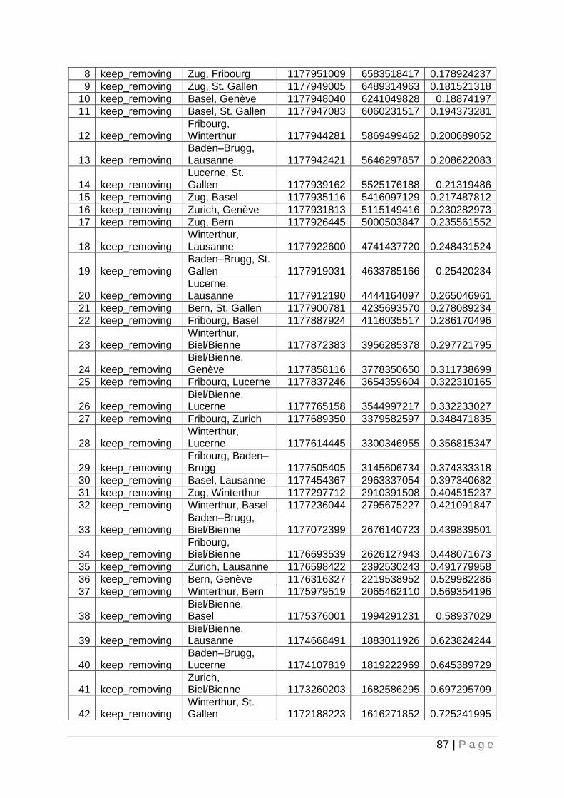
87 | P a g e
8 keep_removing Zug, Fribourg 1177951009 6583518417 0.178924237
9 keep_removing Zug, St. Gallen 1177949005 6489314963 0.181521318
10 keep_removing Basel, Genève 1177948040 6241049828 0.18874197
11 keep_removing Basel, St. Gallen 1177947083 6060231517 0.194373281
12 keep_removing Fribourg, Winterthur 1177944281 5869499462 0.200689052
13 keep_removing Baden–Brugg, Lausanne 1177942421 5646297857 0.208622083
14 keep_removing Lucerne, St. Gallen 1177939162 5525176188 0.21319486
15 keep_removing Zug, Basel 1177935116 5416097129 0.217487812
16 keep_removing Zurich, Genève 1177931813 5115149416 0.230282973
17 keep_removing Zug, Bern 1177926445 5000503847 0.235561552
18 keep_removing Winterthur, Lausanne 1177922600 4741437720 0.248431524
19 keep_removing Baden–Brugg, St. Gallen 1177919031 4633785166 0.25420234
20 keep_removing Lucerne, Lausanne 1177912190 4444164097 0.265046961
21 keep_removing Bern, St. Gallen 1177900781 4235693570 0.278089234
22 keep_removing Fribourg, Basel 1177887924 4116035517 0.286170496
23 keep_removing Winterthur, Biel/Bienne 1177872383 3956285378 0.297721795
24 keep_removing Biel/Bienne, Genève 1177858116 3778350650 0.311738699
25 keep_removing Fribourg, Lucerne 1177837246 3654359604 0.322310165
26 keep_removing Biel/Bienne, Lucerne 1177765158 3544997217 0.332233027
27 keep_removing Fribourg, Zurich 1177689350 3379582597 0.348471835
28 keep_removing Winterthur, Lucerne 1177614445 3300346955 0.356815347
29 keep_removing Fribourg, Baden–Brugg 1177505405 3145606734 0.374333318
30 keep_removing Basel, Lausanne 1177454367 2963337054 0.397340682
31 keep_removing Zug, Winterthur 1177297712 2910391508 0.404515237
32 keep_removing Winterthur, Basel 1177236044 2795675227 0.421091847
33 keep_removing Baden–Brugg, Biel/Bienne 1177072399 2676140723 0.439839501
34 keep_removing Fribourg, Biel/Bienne 1176693539 2626127943 0.448071673
35 keep_removing Zurich, Lausanne 1176598422 2392530243 0.491779958
36 keep_removing Bern, Genève 1176316327 2219538952 0.529982286
37 keep_removing Winterthur, Bern 1175979519 2065462110 0.569354196
38 keep_removing Biel/Bienne, Basel 1175376001 1994291231 0.58937029
39 keep_removing Biel/Bienne, Lausanne 1174668491 1883011926 0.623824244
40 keep_removing Baden–Brugg, Lucerne 1174107819 1819222969 0.645389729
41 keep_removing Zurich, Biel/Bienne 1173260203 1682586295 0.697295709
42 keep_removing Winterthur, St. Gallen 1172188223 1616271852 0.725241995

88 | P a g e
43 keep_removing Lucerne, Basel 1170626319 1511991356 0.774228182
44 keep_removing Fribourg, Genève 1170615470 1375674529 0.850939263
45 keep_removing Bern, Lucerne 1168453000 1285584356 0.908888627
46 keep_removing Baden–Brugg, Winterthur 1167267019 1243445433 0.938736021
47 stop_removing_bca
Baden–Brugg, Bern 1164777310 1125298849 1.035082646
Appendix 7-8 Results of link deletion: ‘with fare’ scenario
iteration remove_link link
network_benefits
network_costs
network_bc_ratio
0 initial_fg NA 1112792093 9386042806 0.118558
1 keep_removing Zug, Lausanne 1112792093 8510410971 0.130757
2 keep_removing Fribourg, St. Gallen 1112792048 7975384058 0.139528
3 keep_removing St. Gallen, Lausanne 1112791965 7664793782 0.145182
4 keep_removing Winterthur, Genève 1112791704 7338244460 0.151643
5 keep_removing Zug, Biel/Bienne 1112791046 7208714961 0.154367
6 keep_removing Lucerne, Genève 1112790453 6953348454 0.160037
7 keep_removing Biel/Bienne, St. Gallen 1112789885 6733341140 0.165266
8 keep_removing Zug, Fribourg 1112788310 6583518417 0.169026
9 keep_removing Zug, St. Gallen 1112786306 6489314963 0.17148
10 keep_removing Basel, Genève 1112785341 6241049828 0.178301
11 keep_removing Basel, St. Gallen 1112784384 6060231517 0.183621
12 keep_removing Fribourg, Winterthur 1112781582 5869499462 0.189587
13 keep_removing Baden–Brugg, Lausanne 1112779722 5646297857 0.197081
14 keep_removing Lucerne, St. Gallen 1112776463 5525176188 0.201401
15 keep_removing Zug, Basel 1112772417 5416097129 0.205457
16 keep_removing Zurich, Genève 1112769114 5115149416 0.217544
17 keep_removing Zug, Bern 1112763746 5000503847 0.22253
18 keep_removing Winterthur, Lausanne 1112759901 4741437720 0.234688
19 keep_removing Baden–Brugg, St. Gallen 1112756332 4633785166 0.24014
20 keep_removing Lucerne, Lausanne 1112749491 4444164097 0.250384
21 keep_removing Bern, St. Gallen 1112738082 4235693570 0.262705
22 keep_removing Winterthur, Biel/Bienne 1112725648 4075943432 0.272998
23 keep_removing Fribourg, Basel 1112712791 3956285378 0.281252
24 keep_removing Biel/Bienne, Genève 1112699142 3778350650 0.294493
25 keep_removing Biel/Bienne, Lucerne 1112659368 3668988264 0.303261
26 keep_removing Fribourg, Lucerne 1112638497 3544997217 0.313862
27 keep_removing Fribourg, Zurich 1112562689 3379582597 0.329201
28 keep_removing Winterthur, Lucerne 1112488050 3300346955 0.337082

89 | P a g e
29 keep_removing Fribourg, Baden–Brugg 1112378940 3145606734 0.353629
30 keep_removing Basel, Lausanne 1112327903 2963337054 0.375363
31 keep_removing Zug, Winterthur 1112173023 2910391508 0.382139
32 keep_removing Fribourg, Biel/Bienne 1111968310 2860378727 0.388749
33 keep_removing Winterthur, Basel 1111906877 2745662446 0.404969
34 keep_removing Baden–Brugg, Biel/Bienne 1111765550 2626127943 0.423348
35 keep_removing Zurich, Lausanne 1111670432 2392530243 0.464642
36 keep_removing Bern, Genève 1111389484 2219538952 0.50073
37 keep_removing Zurich, Biel/Bienne 1110808680 2082902277 0.533299
38 keep_removing Winterthur, Bern 1110477076 1928825436 0.575727
39 keep_removing Biel/Bienne, Basel 1110006886 1857654556 0.597531
40 keep_removing Biel/Bienne, Lausanne 1109319342 1746375252 0.635212
41 keep_removing Baden–Brugg, Lucerne 1108756252 1682586295 0.65896
42 keep_removing Lucerne, Basel 1107436527 1578305798 0.701662
43 keep_removing Winterthur, St. Gallen 1106444106 1511991356 0.731779
44 keep_removing Fribourg, Genève 1106432872 1375674529 0.804284
45 keep_removing Baden–Brugg, Winterthur 1105280314 1333535606 0.828834
46 keep_removing Bern, Lucerne 1102714017 1243445433 0.886821
47 keep_removing Baden–Brugg, Bern 1100245017 1125298849 0.977736
48 stop_removing_bca Zug, Baden–Brugg 1099400561 1075515746 1.022208

90 | P a g e
Appendix 7-9 Adjacency matrix link swapping
Zug Fribourg Baden–Brugg Winterthur Zurich Bern Biel/Bienne Lucerne Basel St. Gallen Lausanne Genève
Zug 0 0 1 0 1 0 0 1 0 0 0 0
Fribourg 0 0 0 0 0 1 0 0 0 0 1 0
Baden–Brugg 1 0 0 0 1 0 0 0 1 0 0 0
Winterthur 0 0 0 0 1 0 0 0 0 0 0 0
Zurich 1 0 1 1 0 1 0 1 1 1 0 0
Bern 0 1 0 0 1 0 1 0 1 0 1 0
Biel/Bienne 0 0 0 0 0 1 0 0 0 0 0 0
Lucerne 1 0 0 0 1 0 0 0 0 0 0 0
Basel 0 0 1 0 1 1 0 0 0 0 0 0
St. Gallen 0 0 0 0 1 0 0 0 0 0 0 0
Lausanne 0 1 0 0 0 1 0 0 0 0 0 1
Genève 0 0 0 0 0 0 0 0 0 0 1 0
Appendix 7-10 Adjacency matrix link deletion
Zug Fribourg Baden–Brugg Winterthur Zurich Bern Biel/Bienne Lucerne Basel
St. Gallen Lausanne Genève
Zug 0 0 1 0 1 0 0 1 0 0 0 0
Fribourg 0 0 0 0 0 1 0 0 0 0 1 0 Baden–Brugg 1 0 0 0 1 0 0 0 1 0 0 0
Winterthur 0 0 0 0 1 0 0 0 0 0 0 0
Zurich 1 0 1 1 0 1 0 1 1 1 0 0
Bern 0 1 0 0 1 0 1 0 1 0 1 0
Biel/Bienne 0 0 0 0 0 1 0 0 0 0 0 0
Lucerne 1 0 0 0 1 0 0 0 0 0 0 0
Basel 0 0 1 0 1 1 0 0 0 0 0 0
St. Gallen 0 0 0 0 1 0 0 0 0 0 0 0
Lausanne 0 1 0 0 0 1 0 0 0 0 0 1
Genève 0 0 0 0 0 0 0 0 0 0 1 0


![PLSS and Ownership Spatial Data Standard - blm.gov · Management [BLM Thesaurus] Administrative and Political Boundaries (boundaries), 003 [International Organization for Standardization](https://img.dokumen.tips/doc/110x75/5cec9f8188c993f4158dbbd6/plss-and-ownership-spatial-data-standard-blmgov-management-blm-thesaurus.jpg)