Physics 509 9

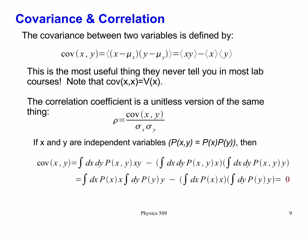
Covariance & Correlation

The covariance between two variables is defined by:

cov x , y=� x��x y�� y�=� xy ��� x � � y �

This is the most useful thing they never tell you in most lab courses! Note that cov(x,x)=V(x).

The correlation coefficient is a unitless version of the same thing:

�=cov x , y

� x� y

If x and y are independent variables (P(x,y) = P(x)P(y)), then

cov x , y=�dx dy P x , y xy � � dx dy P x , y x �dx dy P x , y y

=� dx P x x� dy P y y � �dx P x x� dy P y y = 0

Physics 509 10

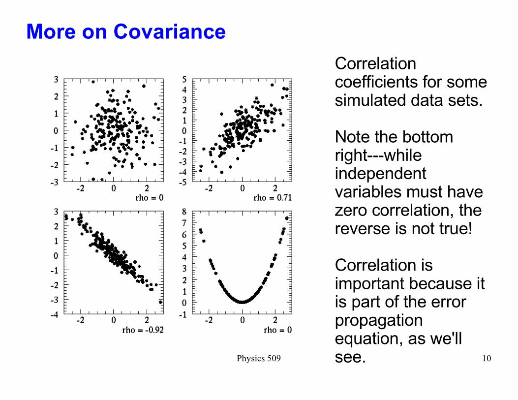
More on Covariance

Correlation coefficients for some simulated data sets.

Note the bottom right---while independent variables must have zero correlation, the reverse is not true!

Correlation is important because it is part of the error propagation equation, as we'll see.

Physics 509 11

Variance and Covariance of Linear Combinations of Variables

Suppose we have two random variable X and Y (not necessarily independent), and that we know cov(X,Y).

Consider the linear combinations W=aX+bY and Z=cX+dY. It can be shown that

cov(W,Z)=cov(aX+bY,cX+dY) = cov(aX,cX) + cov(aX,dY) + cov(bY,cX) + cov(bY,dY)

= ac cov(X,X) + (ad + bc) cov(X,Y) + bd cov(Y,Y) = ac V(X) + bd V(Y) + (ad+bc) cov(X,Y)

Special case is V(X+Y):

V(X+Y) = cov(X+Y,X+Y) = V(X) + V(Y) + 2cov(X,Y)

Very special case: variance of the sum of independent random variables is the sum of their individual variances!

Physics 509 12

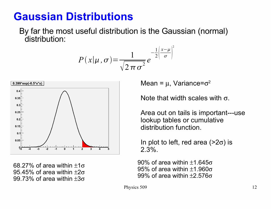
Gaussian Distributions

By far the most useful distribution is the Gaussian (normal) distribution:

P x�� ,�=1

�2��2e�

1

2 x��

� 2

68.27% of area within ±1σ95.45% of area within ±2σ99.73% of area within ±3σ

Mean = µ, Variance=σ2

Note that width scales with σ.

Area out on tails is important---use lookup tables or cumulative distribution function.

In plot to left, red area (>2σ) is 2.3%.

90% of area within ±1.645σ95% of area within ±1.960σ99% of area within ±2.576σ

Physics 509 13

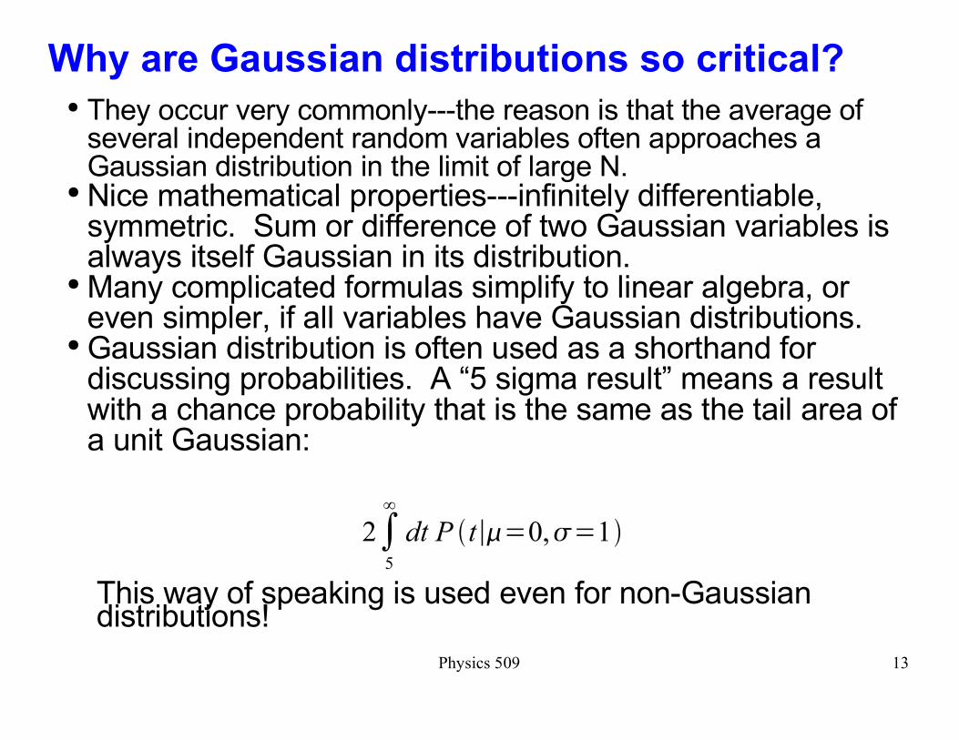
Why are Gaussian distributions so critical?� They occur very commonly---the reason is that the average of

several independent random variables often approaches a Gaussian distribution in the limit of large N.

� Nice mathematical properties---infinitely differentiable, symmetric. Sum or difference of two Gaussian variables is always itself Gaussian in its distribution.

� Many complicated formulas simplify to linear algebra, or even simpler, if all variables have Gaussian distributions.

� Gaussian distribution is often used as a shorthand for discussing probabilities. A �5 sigma result� means a result with a chance probability that is the same as the tail area of a unit Gaussian:

2�5

�

dt P t��=0,�=1

This way of speaking is used even for non-Gaussian distributions!

Physics 509 14

Why you should be very careful with Gaussians ..

The major danger of Gaussians is that they are overused. Although many distributions are approximately Gaussian, they often have long non-Gaussian tails.

While 99% of the time a Gaussian distribution will correctly model your data, many foul-ups result from that other 1%.

It's usually good practice to simulate your data to see if the distributions of quantities you think are Gaussian really follow a Gaussian distribution.

Common example: the ratio of two numbers with Gaussian distributions is itself often not very Gaussian (although in certain limits it may be).

Physics 509 10

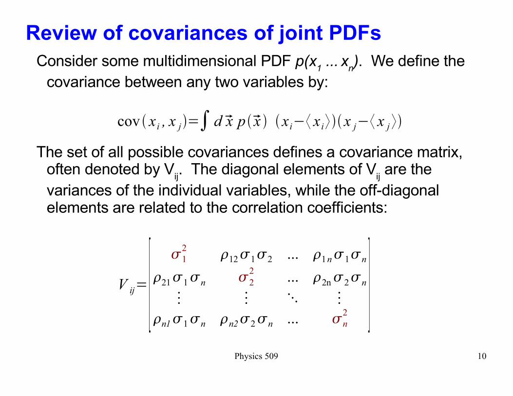
Review of covariances of joint PDFs

Consider some multidimensional PDF p(x1 ...

x

n). We define the

covariance between any two variables by:

cov � xi , x j�=� d �x p��x � �xi� xi���x j� x j ��

The set of all possible covariances defines a covariance matrix, often denoted by V

ij. The diagonal elements of V

ij are the

variances of the individual variables, while the off-diagonal elements are related to the correlation coefficients:

V ij=[�1

2 �12�1�2 ... �1n�1�n

�21�1�n �2

2... �2n�2�n

� � � �

�n1�1�n �n2�2�n ... �n

2 ]

Physics 509 11

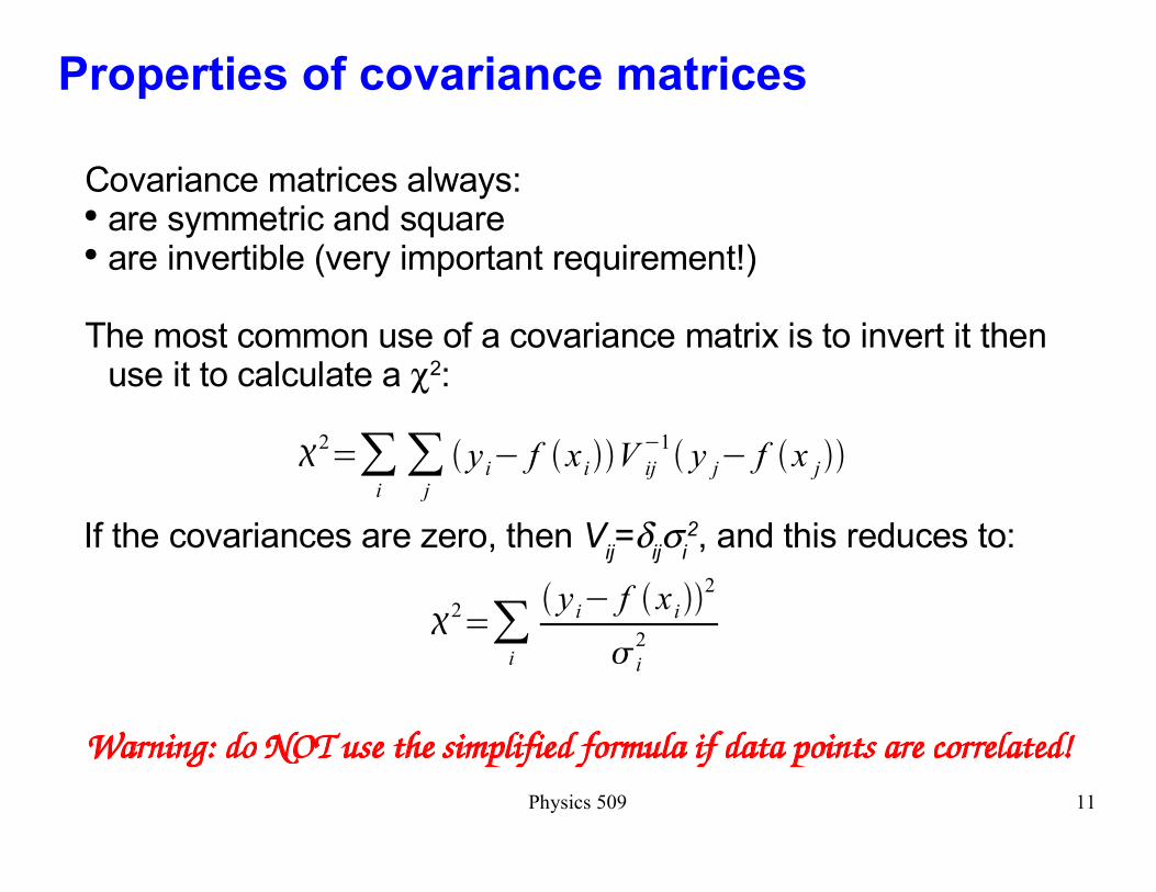
Properties of covariance matrices

Covariance matrices always:� are symmetric and square� are invertible (very important requirement!)

The most common use of a covariance matrix is to invert it then use it to calculate a χ2:

�2=�i

�j

� yi f �xi��V ij

1� y j f �x j��

If the covariances are zero, then Vij=δ

ijσ

i2, and this reduces to:

�2=�i

� yi f �xi��2

� i

2

Warning: do NOT use the simplified formula if data points are correlated!

Physics 509 12

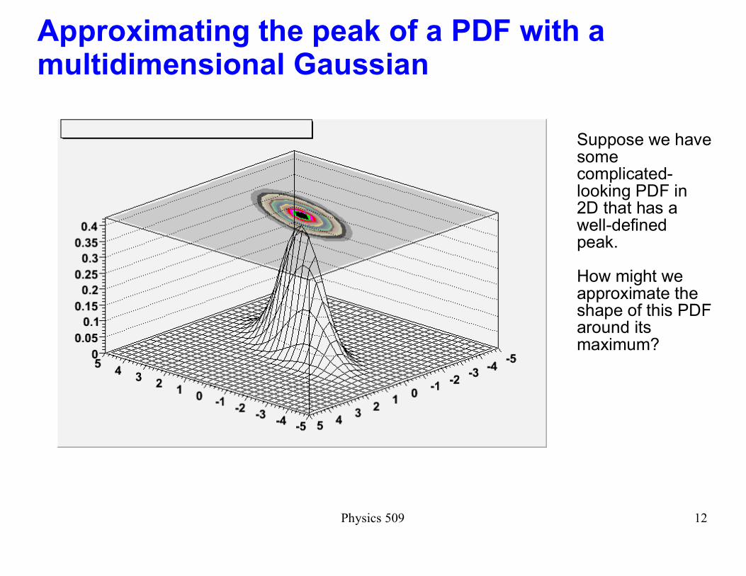
Approximating the peak of a PDF with a multidimensional Gaussian

Suppose we have some complicated-looking PDF in 2D that has a well-defined peak.

How might we approximate the shape of this PDF around its maximum?

Physics 509 13

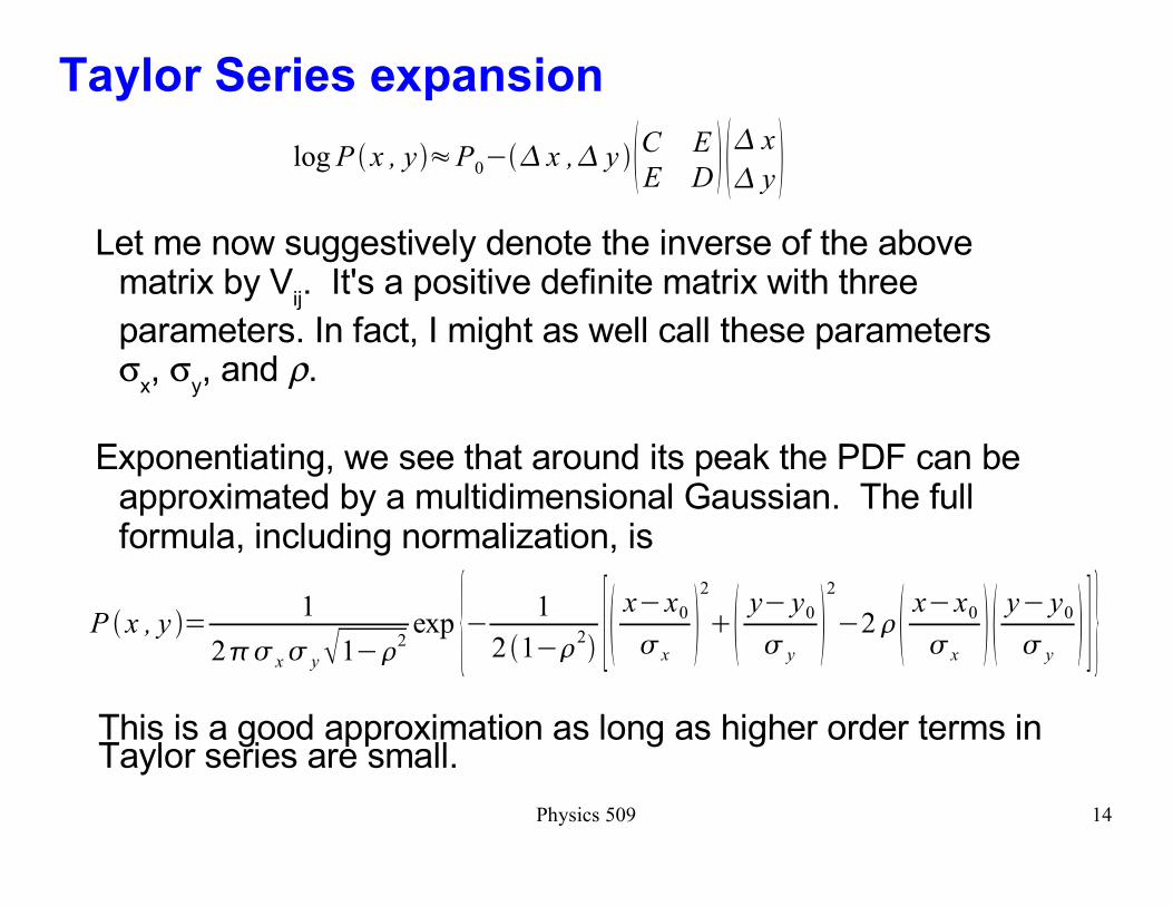
Taylor Series expansion

Consider a Taylor series expansion of the logarithm of the PDF around its maximum at (x

0,y

0):

log P � x , y�=P0�A� xx0��B � y y0�C � xx0�2D � y y0�

22E � xx0�� y y0� ...

Since we are expanding around the peak, then the first derivatives must equal zero, so A=B=0. The remaining terms can be written in matrix form:

log P � x , y��P0�� x ,� y ��C E

E D � �� x� y �In order for (x

0,y

0) to be a maximum of the PDF (and not a

minimum or saddle point), the above matrix must be positive definite, and therefore invertible.

Physics 509 14

Taylor Series expansion

Let me now suggestively denote the inverse of the above matrix by V

ij. It's a positive definite matrix with three

parameters. In fact, I might as well call these parameters σ

x, σ

y, and ρ.

Exponentiating, we see that around its peak the PDF can be approximated by a multidimensional Gaussian. The full formula, including normalization, is

log P � x , y��P0�� x ,� y ��C E

E D � �� x� y �

P � x , y �=1

2�� x� y�1�2exp { 1

2 �1�2� [� xx0

� x�2

�� y y0

� y�2

2�� xx0

� x� � y y0

� y� ] }

This is a good approximation as long as higher order terms in Taylor series are small.

Physics 509 15

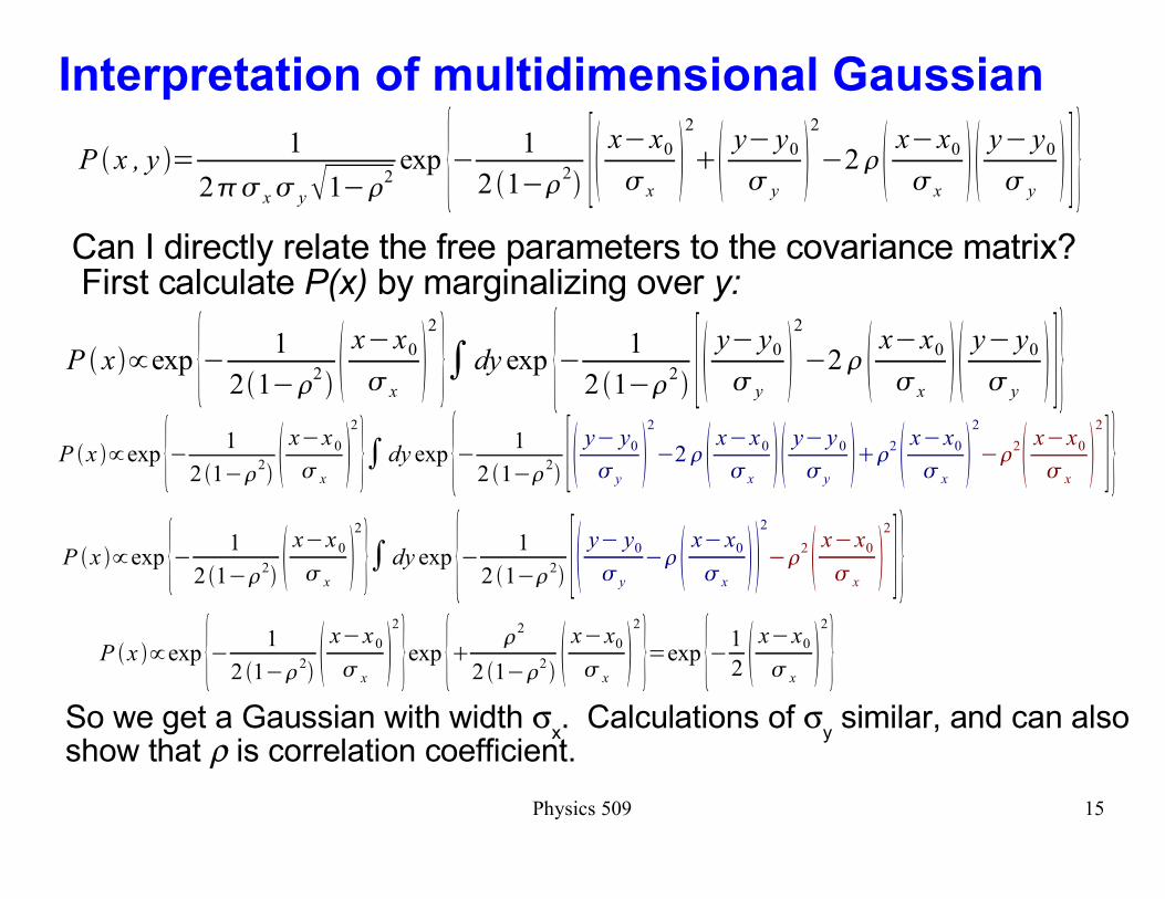
Interpretation of multidimensional Gaussian

P � x , y �=1

2�� x� y�1�2exp { 1

2 �1�2� [� xx0

� x�2

�� y y0

� y�2

2�� xx0

� x� � y y0

� y� ] }

Can I directly relate the free parameters to the covariance matrix? First calculate P(x) by marginalizing over y:

P � x��exp { 1

2�1�2� �xx0

� x�2

}�dy exp { 1

2 �1�2� [ � y y0

� y�2

2� � xx0

� x� � y y0

� y� ]}

P �x ��exp { 1

2 �1�2� �xx0

� x�2

}� dy exp { 1

2 �1�2� [� y y0

� y�2

2�� xx0

� x� � y y0

� y���2 � xx0

� x�2

�2� xx0

� x�2

]}P �x ��exp { 1

2 �1�2� �xx0

� x�2

}� dy exp { 1

2 �1�2� [� y y0

� y

�� xx0

� x� �

2

�2 � xx0

� x�2

]}P �x ��exp { 1

2 �1�2� �xx0

� x�2

}exp {� �2

2 �1�2� �xx0

� x�2

}=exp {1

2 � xx0

� x�2

}So we get a Gaussian with width σ

x. Calculations of σ

y similar, and can also

show that ρ is correlation coefficient.

Physics 509 16

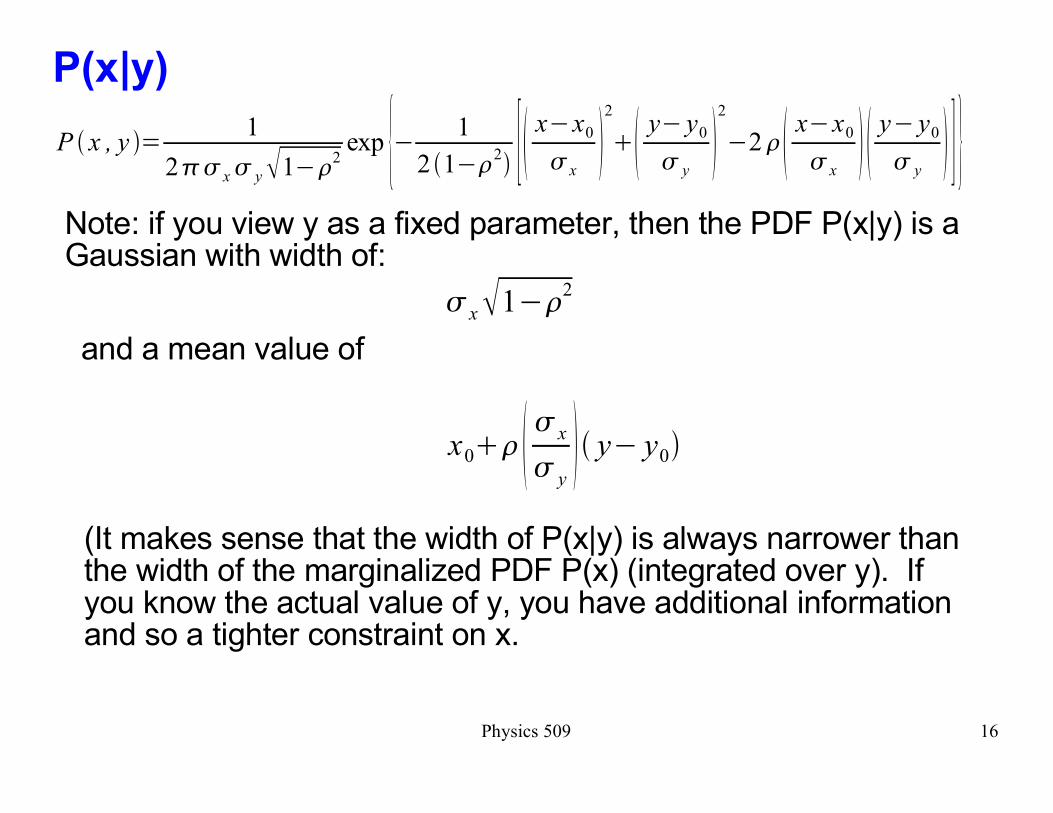
P(x|y)

P � x , y �=1

2�� x� y�1�2exp { 1

2 �1�2� [� xx0

� x�2

�� y y0

� y�2

2�� xx0

� x� � y y0

� y� ] }

Note: if you view y as a fixed parameter, then the PDF P(x|y) is a Gaussian with width of:

� x�1�2

and a mean value of

x0��� � x

� y� � y y0�

(It makes sense that the width of P(x|y) is always narrower than the width of the marginalized PDF P(x) (integrated over y). If you know the actual value of y, you have additional information and so a tighter constraint on x.

Physics 509 17

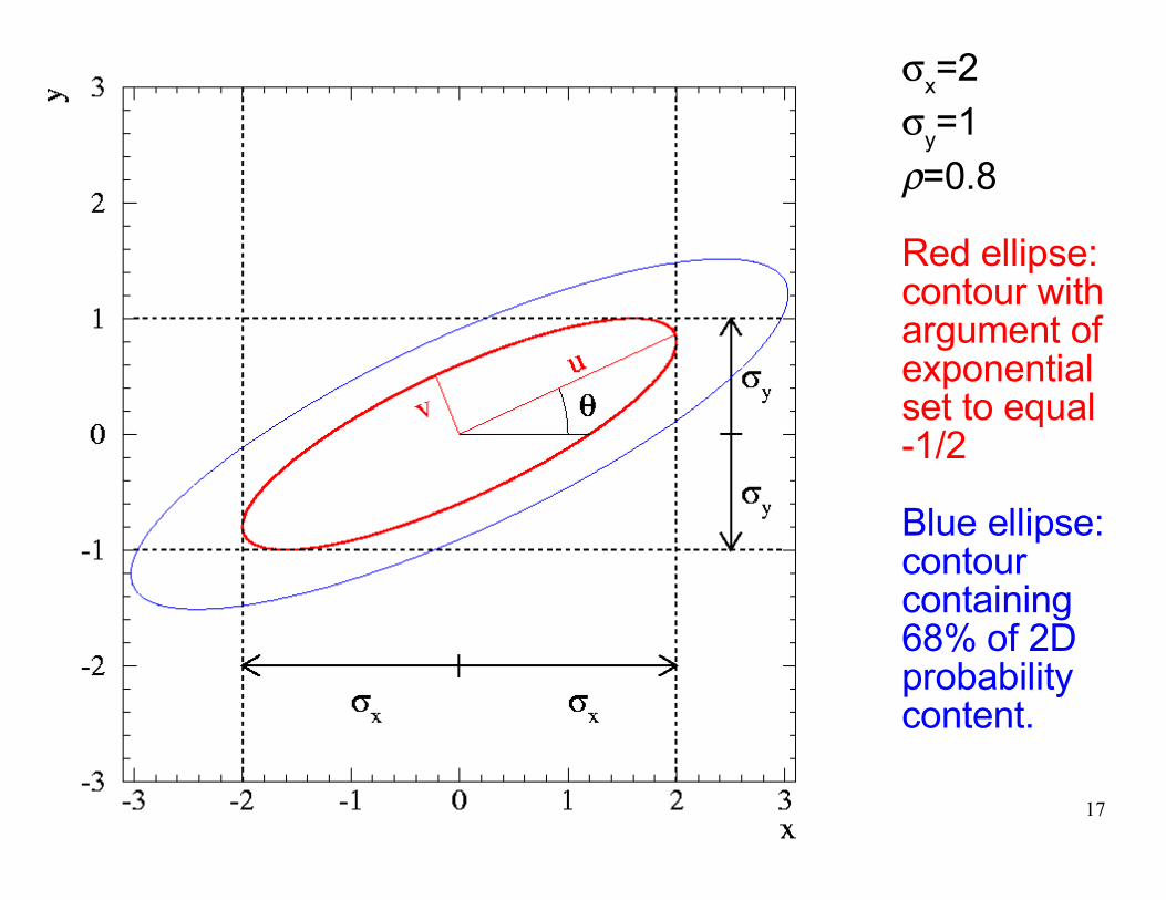
σx=2

σy=1

ρ=0.8

Red ellipse: contour with argument of exponential set to equal -1/2

Blue ellipse: contour containing 68% of 2D probability content.

Physics 509 18

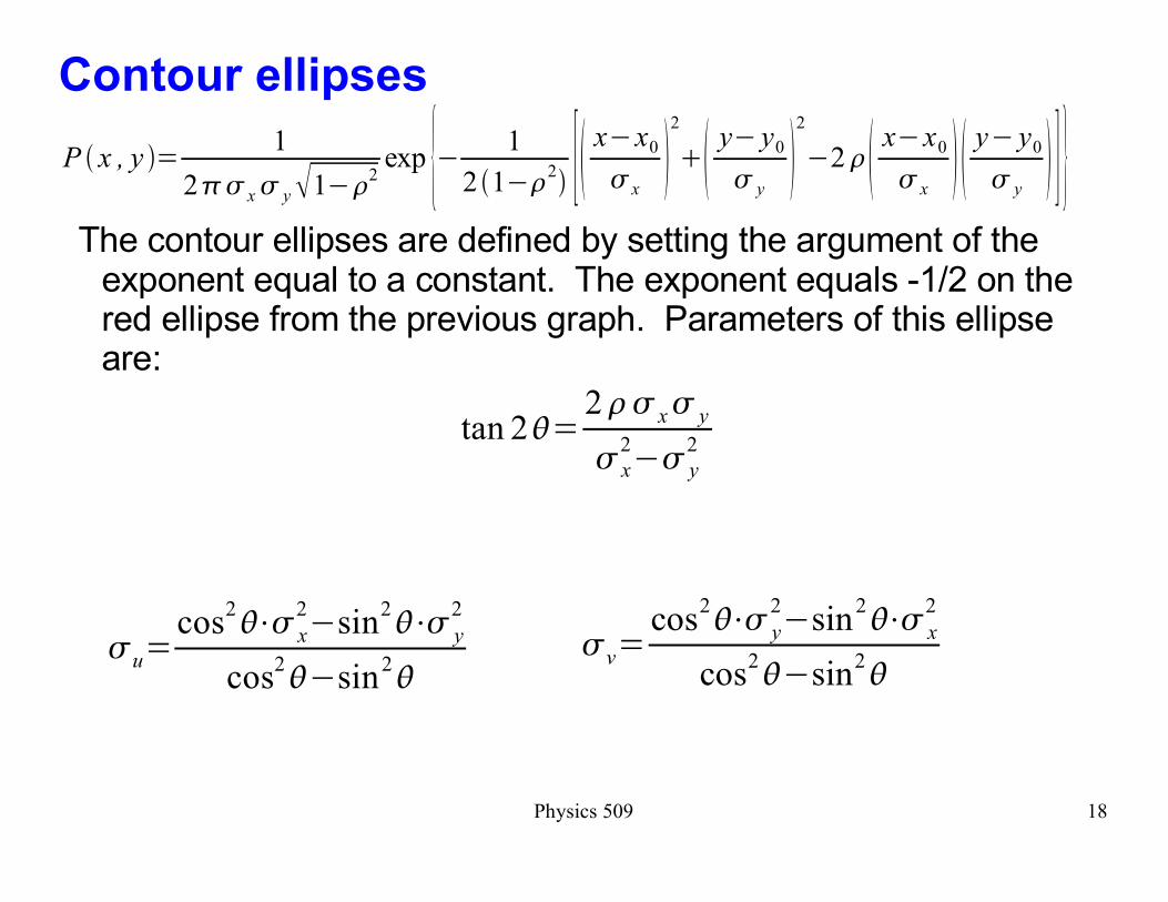
Contour ellipses

The contour ellipses are defined by setting the argument of the exponent equal to a constant. The exponent equals -1/2 on the red ellipse from the previous graph. Parameters of this ellipse are:

P � x , y �=1

2�� x� y�1�2exp { 1

2 �1�2� [� xx0

� x�2

�� y y0

� y�2

2�� xx0

� x� � y y0

� y� ] }

tan 2�=2�� x� y

� x

2� y

2

�u=cos

2��� x

2sin2��� y

2

cos2�sin

2��v=

cos2��� y

2sin2��� x

2

cos2�sin

2�

Physics 509 19

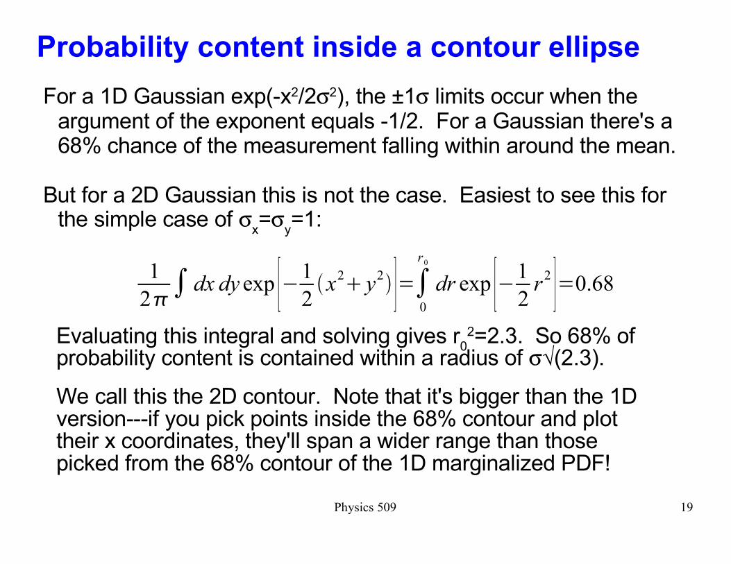
Probability content inside a contour ellipse

For a 1D Gaussian exp(-x2/2σ2), the ±1σ limits occur when the argument of the exponent equals -1/2. For a Gaussian there's a 68% chance of the measurement falling within around the mean.

But for a 2D Gaussian this is not the case. Easiest to see this for the simple case of σ

x=σ

y=1:

1

2�� dx dy exp [1

2�x2� y2� ]=�

0

r0

dr exp [1

2r

2 ]=0.68

Evaluating this integral and solving gives r02=2.3. So 68% of

probability content is contained within a radius of σ�(2.3).

We call this the 2D contour. Note that it's bigger than the 1D version---if you pick points inside the 68% contour and plot their x coordinates, they'll span a wider range than those picked from the 68% contour of the 1D marginalized PDF!

Physics 509 20

σx=2

σy=1

ρ =0.8

Red ellipse: contour with argument of exponential set to equal -1/2

Blue ellipse: contour containing 68% of probability content.

Physics 509 21

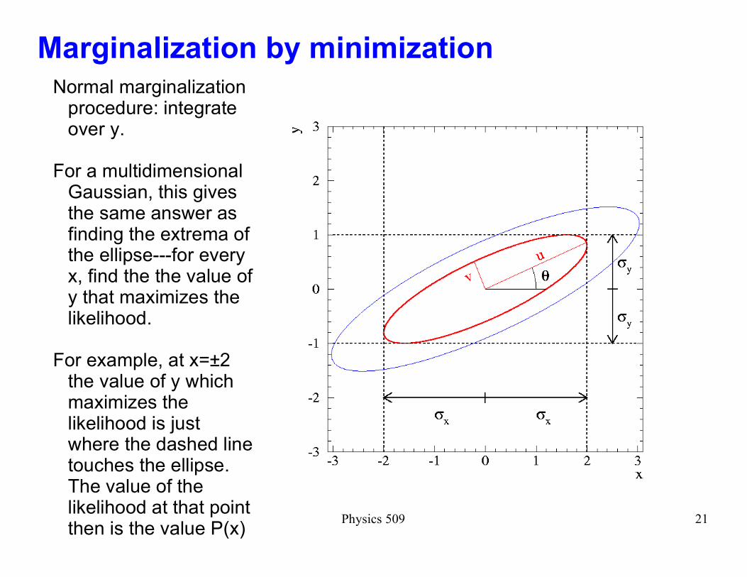
Marginalization by minimizationNormal marginalization

procedure: integrate over y.

For a multidimensional Gaussian, this gives the same answer as finding the extrema of the ellipse---for every x, find the the value of y that maximizes the likelihood.

For example, at x=±2 the value of y which maximizes the likelihood is just where the dashed line touches the ellipse. The value of the likelihood at that point then is the value P(x)

Physics 509 22

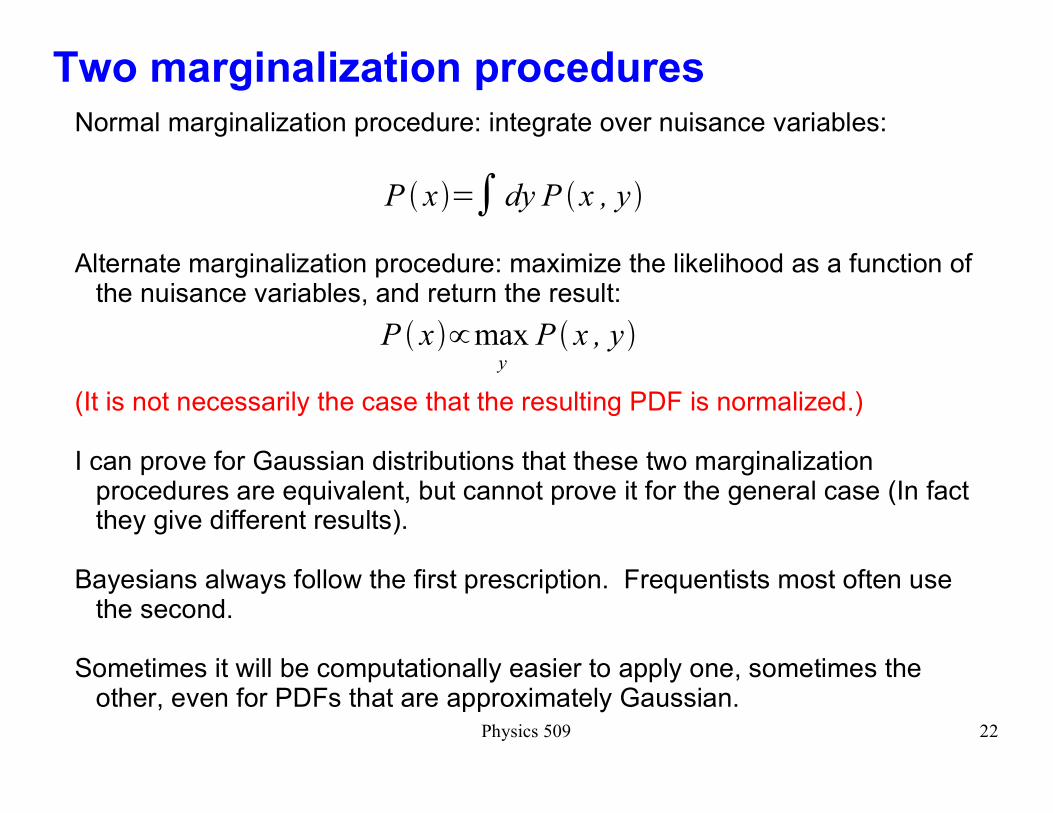
Two marginalization proceduresNormal marginalization procedure: integrate over nuisance variables:

P � x�=� dy P �x , y�

Alternate marginalization procedure: maximize the likelihood as a function of the nuisance variables, and return the result:

P � x��maxy

P � x , y�

(It is not necessarily the case that the resulting PDF is normalized.)

I can prove for Gaussian distributions that these two marginalization procedures are equivalent, but cannot prove it for the general case (In fact they give different results).

Bayesians always follow the first prescription. Frequentists most often use the second.

Sometimes it will be computationally easier to apply one, sometimes the other, even for PDFs that are approximately Gaussian.

Physics 509 12

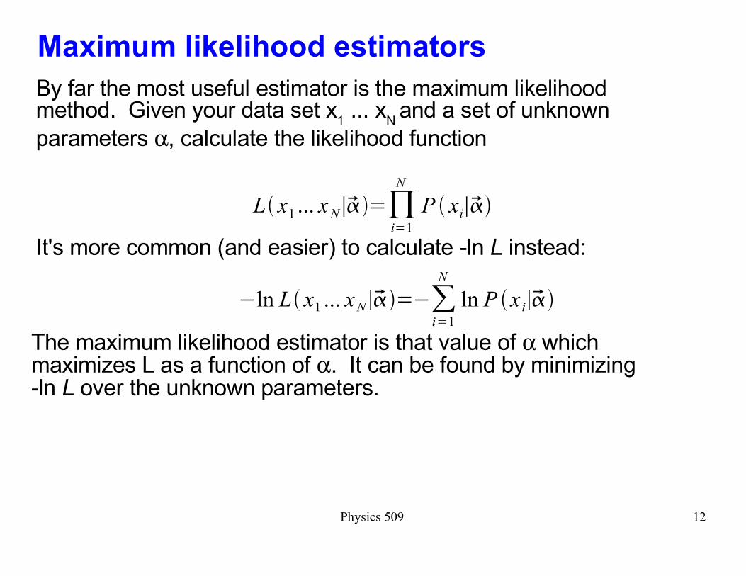
Maximum likelihood estimators

By far the most useful estimator is the maximum likelihood method. Given your data set x

1 ... x

N and a set of unknown

parameters α, calculate the likelihood function

L� x1 ... xN����=�i=1

N

P � xi����

It's more common (and easier) to calculate -ln L instead:

ln L� x1 ... xN����=�i=1

N

ln P �xi����

The maximum likelihood estimator is that value of α which maximizes L as a function of α. It can be found by minimizing -ln L over the unknown parameters.

Physics 509 13

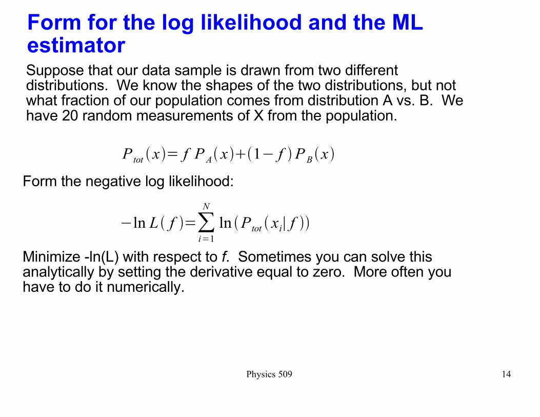
Simple example of an ML estimator

Suppose that our data sample is drawn from two different distributions. We know the shapes of the two distributions, but not what fraction of our population comes from distribution A vs. B. We have 20 random measurements of X from the population.

PA�x�=2

1e2e2x

PB �x�=3x2

Ptot � x�= f PA� x���1 f �PB �x�

Physics 509 14

Form for the log likelihood and the ML estimatorSuppose that our data sample is drawn from two different distributions. We know the shapes of the two distributions, but not what fraction of our population comes from distribution A vs. B. We have 20 random measurements of X from the population.

Ptot � x�= f PA� x���1 f �PB �x�

Form the negative log likelihood:

Minimize -ln(L) with respect to f. Sometimes you can solve this analytically by setting the derivative equal to zero. More often you have to do it numerically.

ln L � f �=�i=1

N

ln �Ptot � xi� f ��

Physics 509 15

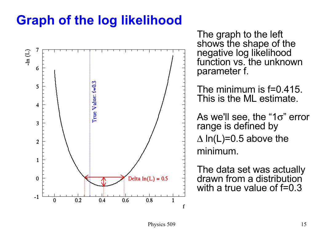
Graph of the log likelihoodThe graph to the left shows the shape of the negative log likelihood function vs. the unknown parameter f.

The minimum is f=0.415. This is the ML estimate.

As we'll see, the �1σ� error range is defined by

∆ ln(L)=0.5 above the

minimum.

The data set was actually drawn from a distribution with a true value of f=0.3

Physics 509 18

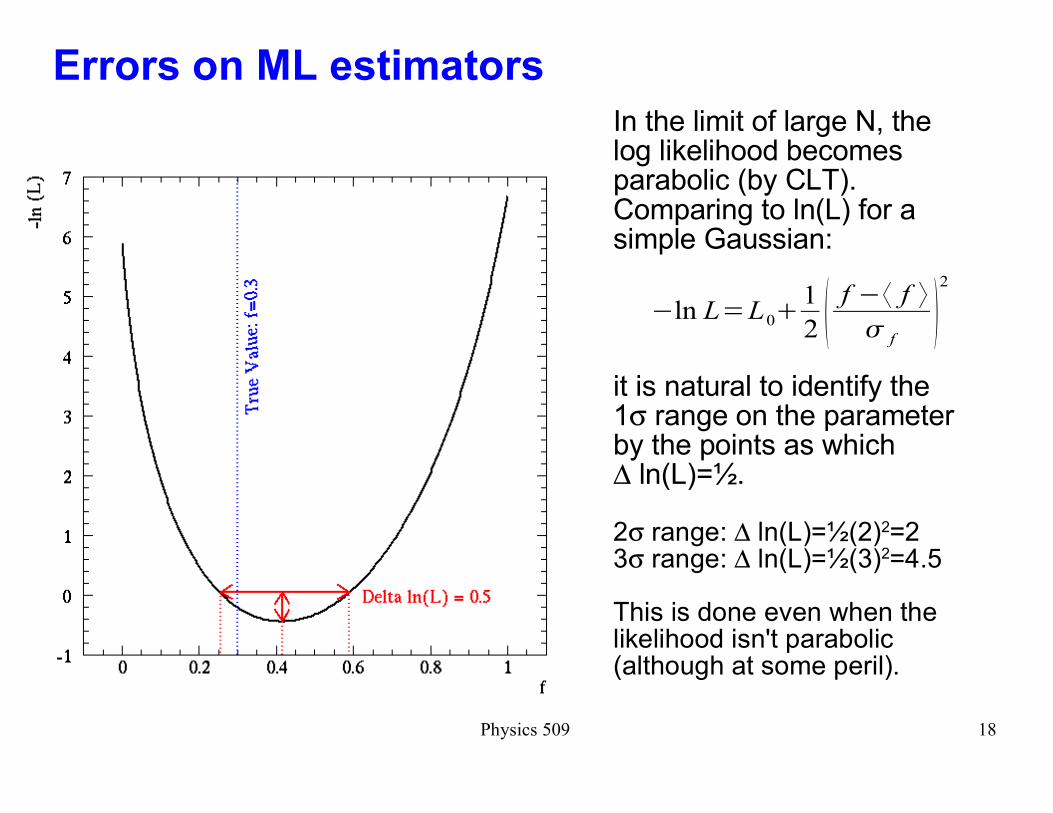
Errors on ML estimators

In the limit of large N, the log likelihood becomes parabolic (by CLT). Comparing to ln(L) for a simple Gaussian:

it is natural to identify the 1σ range on the parameter by the points as which ∆ ln(L)=½.

2σ range: ∆ ln(L)=½(2)2=23σ range: ∆ ln(L)=½(3)2=4.5

This is done even when the likelihood isn't parabolic (although at some peril).

ln L=L0�1

2 � f � f

f�2

Physics 509 19

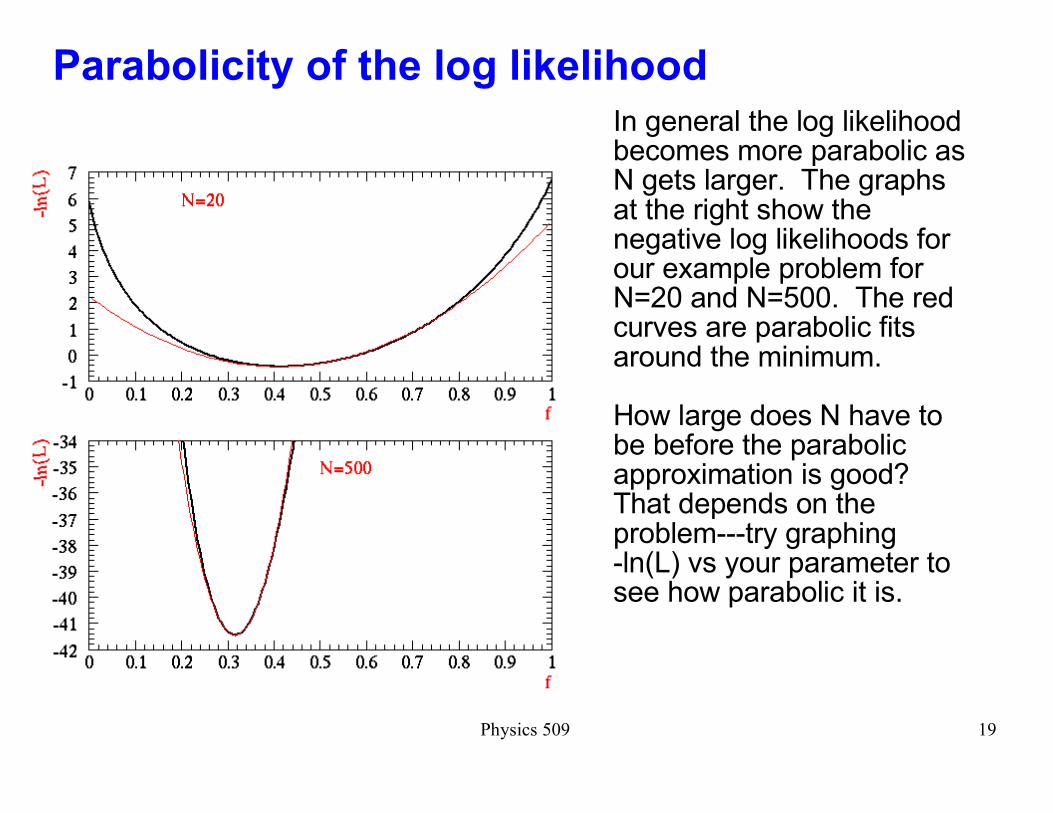
Parabolicity of the log likelihood

In general the log likelihood becomes more parabolic as N gets larger. The graphs at the right show the negative log likelihoods for our example problem for N=20 and N=500. The red curves are parabolic fits around the minimum.

How large does N have to be before the parabolic approximation is good? That depends on the problem---try graphing -ln(L) vs your parameter to see how parabolic it is.

Physics 509 20

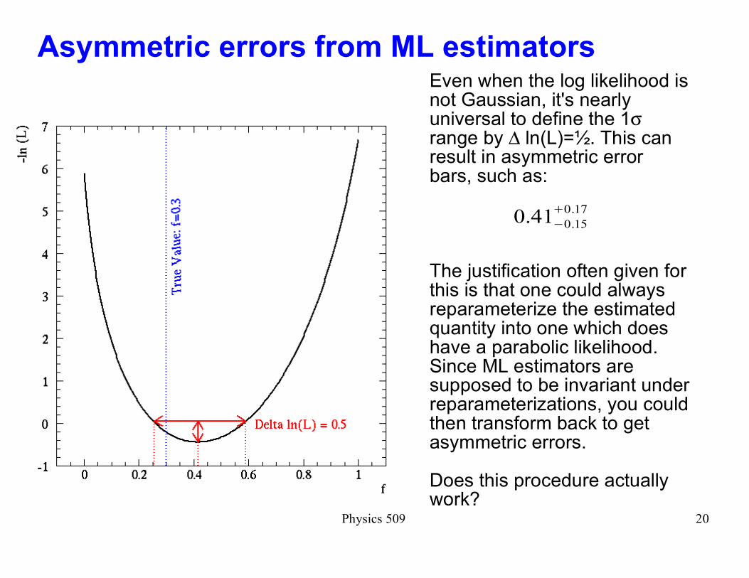
Asymmetric errors from ML estimatorsEven when the log likelihood is not Gaussian, it's nearly universal to define the 1σ range by ∆ ln(L)=½. This can result in asymmetric error bars, such as:

The justification often given for this is that one could always reparameterize the estimated quantity into one which does have a parabolic likelihood. Since ML estimators are supposed to be invariant under reparameterizations, you could then transform back to get asymmetric errors.

Does this procedure actually work?

0.410.15

�0.17

Physics 509 21

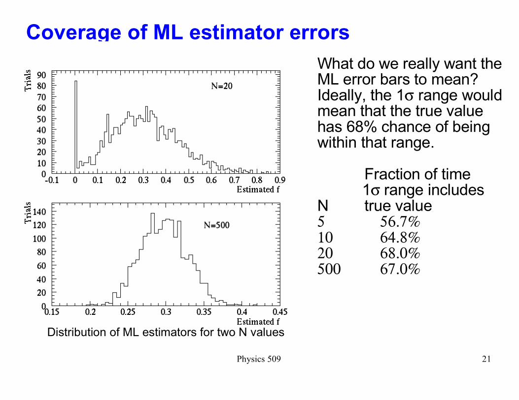
Coverage of ML estimator errors

What do we really want the ML error bars to mean? Ideally, the 1σ range would mean that the true value has 68% chance of being within that range.

Fraction of time 1σ range includes

N true value5 56.7%10 64.8%20 68.0%500 67.0%

Distribution of ML estimators for two N values

Physics 509 22

Errors on ML estimators

Simulation is the best way to estimate the true error range on an ML estimator: assume a true value for the parameter, and simulate a few hundred experiments, then calculate ML estimates for each.

N=20:Range from likelihood function: -0.16 / +0.17RMS of simulation: 0.16

N=500:Range from likelihood function: -0.030 / +0.035RMS of simulation: 0.030

Physics 509 23

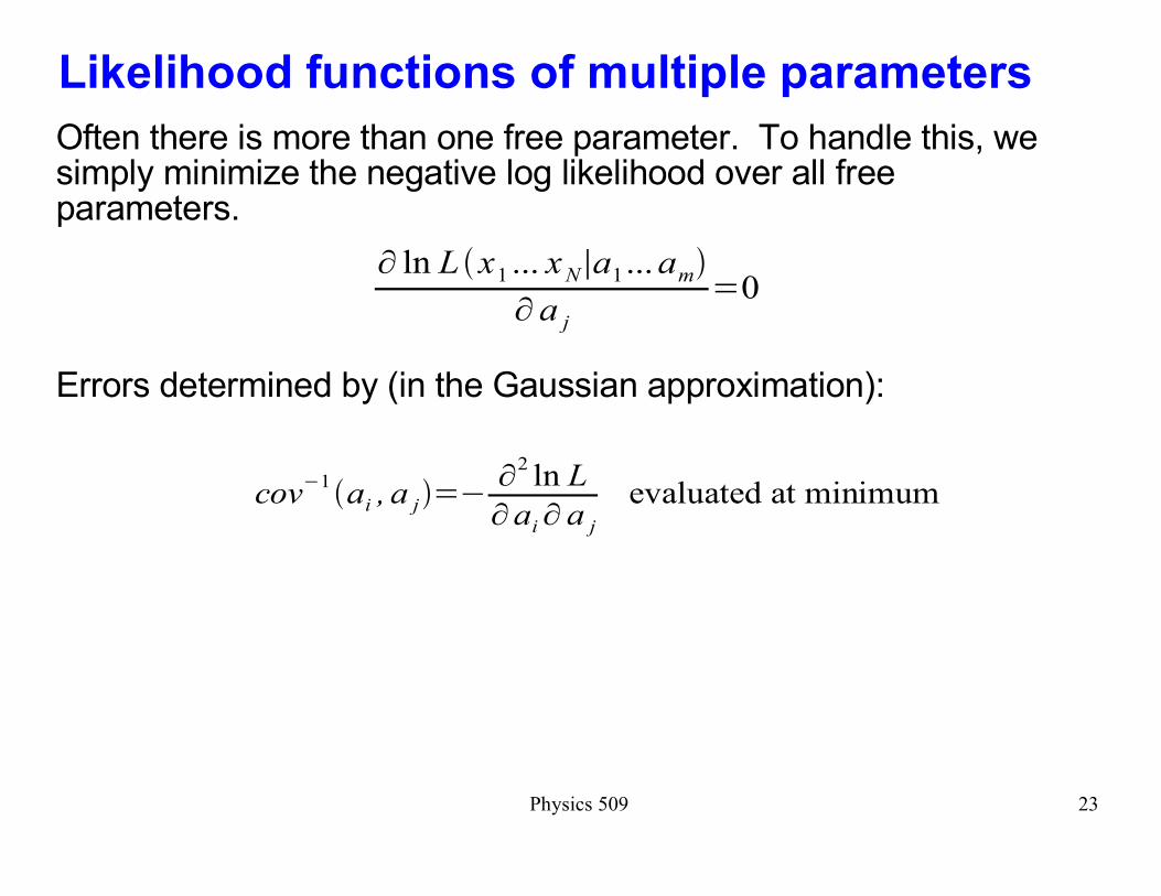
Likelihood functions of multiple parameters

Often there is more than one free parameter. To handle this, we simply minimize the negative log likelihood over all free parameters.

Errors determined by (in the Gaussian approximation):

� ln L �x1 ... xN�a1...am�

� a j=0

cov1�ai , a j�=

�2ln L

�ai� a j evaluated at minimum

Physics 509 24

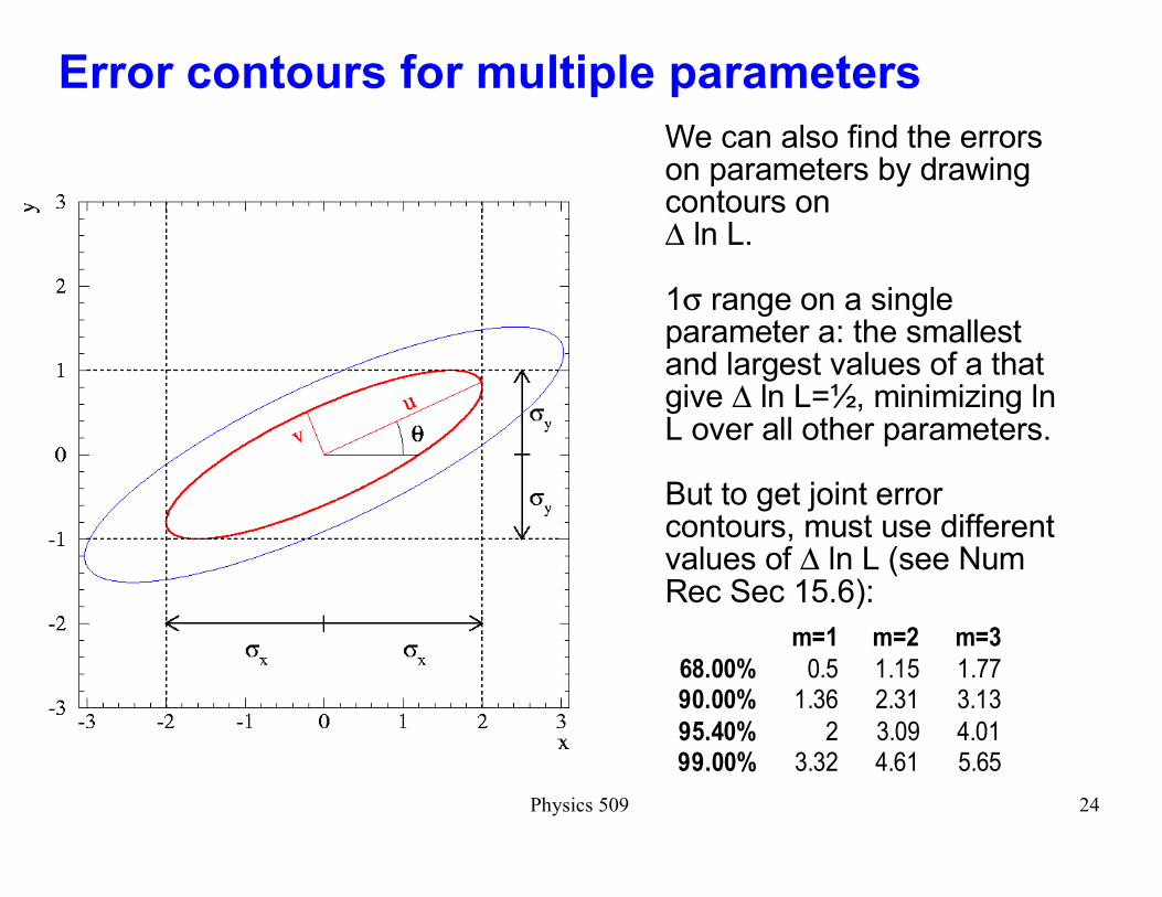
Error contours for multiple parameters

We can also find the errors on parameters by drawing contours on ∆ ln L.

1σ range on a single parameter a: the smallest and largest values of a that give ∆ ln L=½, minimizing ln L over all other parameters.

But to get joint error contours, must use different values of ∆ ln L (see Num Rec Sec 15.6):

m=1 m=2 m=3

68.00% 0.5 1.15 1.7790.00% 1.36 2.31 3.13

95.40% 2 3.09 4.0199.00% 3.32 4.61 5.65

Physics 509 3

Maximum Likelihood with Gaussian Errors

Suppose we want to fit a set of points (xi,y

i) to some model

y=f(x|α), in order to determine the parameter(s) α. Often the measurements will be scattered around the model with some Gaussian error. Let's derive the ML estimator for α.

The log likelihood is then

Maximizing this is equivalent to minimizing

L=�i=1

N1

� i�2�exp [�1

2 � yi� f �xi�� i2

]ln L=�

1

2�i=1

N

� yi� f �xi��i 2

��i=1

N

ln �� i�2�

�2=�i=1

N

� yi� f �xi�� i2

Physics 509 4

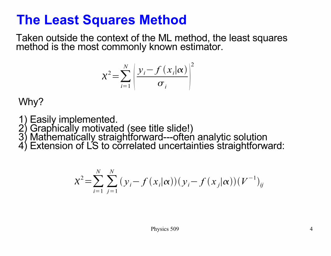
The Least Squares Method

Taken outside the context of the ML method, the least squares method is the most commonly known estimator.

�2=�i=1

N

� yi� f �xi�� i2

Why?

1) Easily implemented.2) Graphically motivated (see title slide!)3) Mathematically straightforward---often analytic solution4) Extension of LS to correlated uncertainties straightforward:

�2=�i=1

N

�j=1

N

� yi� f �xi�� yi� f �x j��V�1ij

Physics 509 5

Least Squares Straight Line Fit

The most straightforward example is a linear fit: y=mx+b.

�2=�� yi�mxi�b�i

2

Least squares estimators for m and b are found by differentiating χ2 with respect to m & b.

d �2

dm=�2�� yi�mxi�b� i

2 xi=0

d �2

db=�2�� yi�mxi�b� i

2 =0

This is a linear system of simultaneous equations with two unknowns.

Physics 509 6

Solving for m and b

The most straightforward example is a linear fit: y=mx+b.

d �2

dm=�2�� yi�mxi�b� i

2 xi=0d �2

db=�2�� yi�mxi�b� i

2 =0

�m=�� yi

� i

2 �� xi

� i

2 ��� 1

� i

2 �� xi yi

� i

2 �� xi

� i

2 2

��� xi2

� i

2 �� 1

� i

2 � �m= � y � � x ��� xy �

� x �2�� x

2�

� � yi� i

2 =m� � xi� i

2 �b�� 1

�i2 � � xi yi� i

2 =m�� xi2

� i

2 �b�� xi� i2

�b=�� yi

�i2 � �m �� xi

� i

2 �� 1

� i

2 � �b=� y �� �m� x �

(Special case of equal σ's.)

Physics 509 7

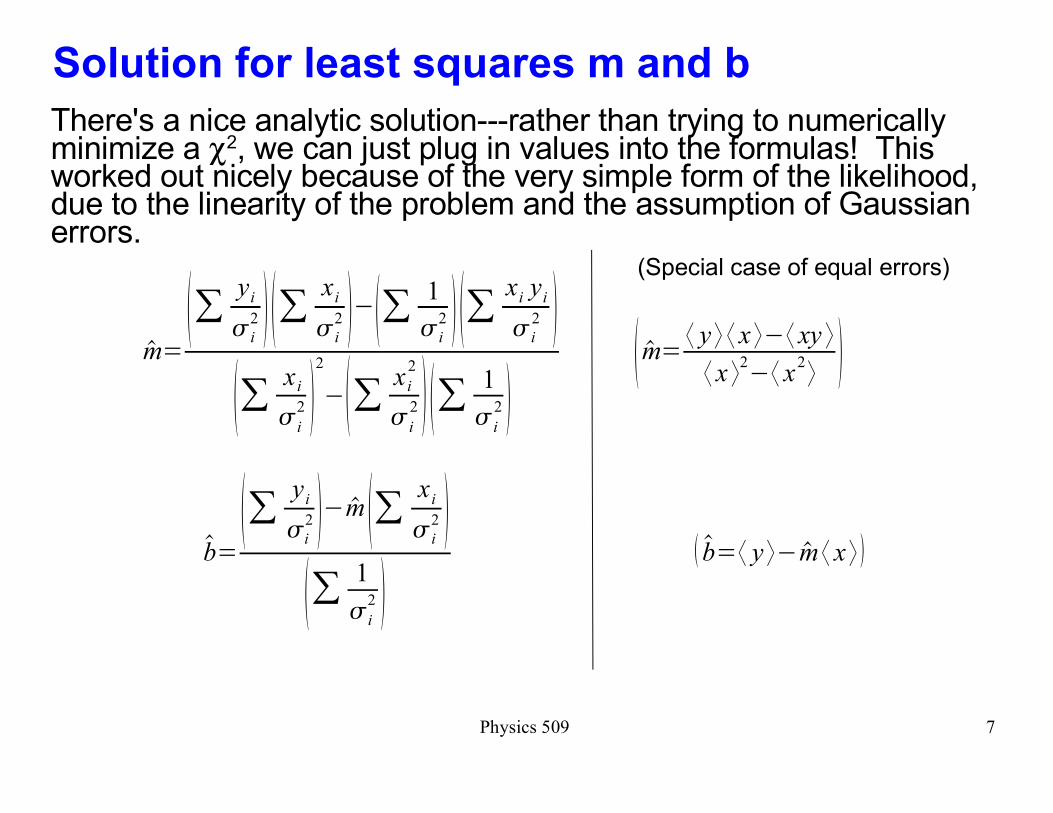
Solution for least squares m and b

There's a nice analytic solution---rather than trying to numerically minimize a χ2, we can just plug in values into the formulas! This worked out nicely because of the very simple form of the likelihood, due to the linearity of the problem and the assumption of Gaussian errors.

�m=�� yi

� i

2 �� xi

� i

2 ��� 1

� i

2 �� xi yi

� i

2 �� xi

� i

2 2

��� xi2

� i

2 �� 1

� i

2 � �m= � y � � x ��� xy �

� x �2�� x

2�

�b=�� yi

�i2 � �m �� xi

� i

2 �� 1

� i

2 � �b=� y �� �m� x �

(Special case of equal errors)

Physics 509 8

Errors in the Least Squares Method

What about the errors and correlations between m and b? Simplest way to derive this is to look at the chi-squared, and remember that this is a special case of the ML method:

�ln L=1

2�2=

1

2�� yi�mxi�b� i

2

In the ML method, we define the 1σ error on a parameter by the minimum and maximum value of that parameter satisfying

∆ ln L=½.

In LS method, this corresponds to ∆χ2=+1 above the best-fit point. Two sigma error range corresponds to ∆χ2=+4, 3σ is ∆χ2=+9, etc.

But notice one thing about the dependence of the χ2---it is quadratic in both m and b, and generally includes a cross-term proportional to mb. Conclusion: Gaussian uncertainties on m and b, with a covariance between them.

Physics 509 10

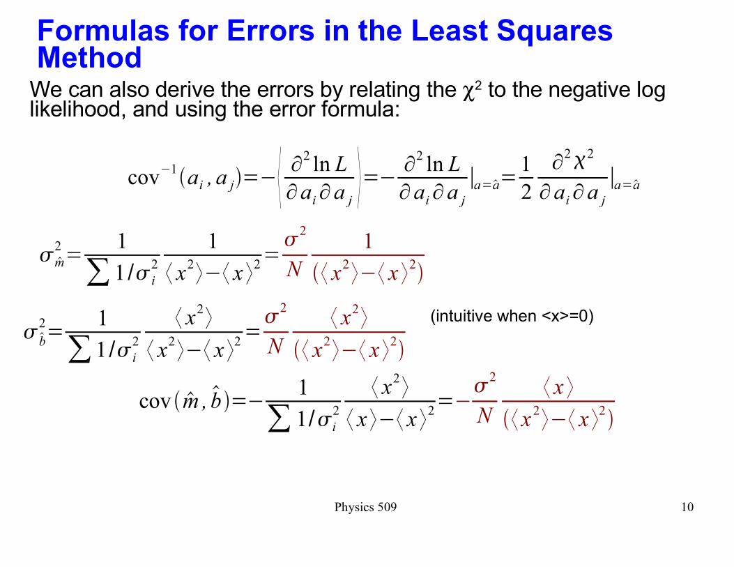
Formulas for Errors in the Least Squares Method

We can also derive the errors by relating the χ2 to the negative log likelihood, and using the error formula:

� �m2=

1

� 1 /� i

2

1

� x2��� x �2=�2

N

1

�� x2��� x �2

��b

2=

1

� 1 /� i

2

� x2�

� x2��� x �2=�2

N

� x2�

�� x2��� x �2

cov � �m , �b=�1

� 1/�i2

� x2�

� x ��� x �2=�

�2

N

� x �

�� x2��� x �2

(intuitive when <x>=0)

cov�1�ai , a j=�� �

2ln L

�ai�a j �=��2

ln L

�ai�a j�a=�a=

1

2

�2�2

�ai�a j�a=�a

Physics 509 18

Nonlinear least squares

The derivation of the least squares method doesn't depend on the assumption that your fitting function is linear in the parameters. Nonlinear fits, such as A + B sin(Ct + D), can be tackled with the least squares technique as well. But things aren't nearly as nice:

� No closed form solution---have to minimize the χ2 numerically.� Estimators are no longer guaranteed to have zero bias and minimum variance.� Contours generated by ∆χ2=+1 no longer are ellipses, and the tangents to these contours no longer give the standard deviations. (However, we can still interpret them as giving �1σ� errors---although since the distribution is non-Gaussian, this error range isn't the same thing as a standard deviation� Be very careful with minimization routines---depending on how badly non-linear your problem is, there may be multiple solutions, local minima, etc.

Physics 509 19

Goodness of fit for least squares

By now you're probably wondering why I haven't discussed the use of χ2 as a goodness of fit parameter. Partly this is because parameter estimation and goodness of fit are logically separate things---if you're CERTAIN that you've got the correct model and error estimates, then a poor χ2 can only be bad luck, and tells you nothing about how accurate your parameter estimates are.

Carefully distinguish between:

1) Value of χ2 at minimum: a measure of goodness of fit2) How quickly χ2 changes as a function of the parameter: a measure of the uncertainty on the parameter.

Nonetheless, a major advantage of the χ2 approach is that it does automatically generate a goodness of fit parameter as a byproduct of the fit. As we'll see, the maximum likelihood method doesn't.

How does this work?

Physics 509 20

χ2 as a goodness of fit parameter

Remember that the sum of N Gaussian variables with zero mean and unit RMS, when squared and added, follows a χ2 distribution with N degrees of freedom. Compare to the least squares formula:

�2=�

i

�j

� yi� f �xi�� y j� f �x j��V�1ij

If each yi is distributed around the function according to a

Gaussian, and f(x|α) is a linear function of the m free parameters α, and the error estimates don't depend on the free parameters, then the best-fit least squares quantity we call χ2 actually follows a χ2 distribution with N-m degrees of freedom.

People usually ignore these various caveats and assume this works even when the parameter dependence is non-linear and the errors aren't Gaussian. Be very careful with this, and check with simulation if you're not sure.

Physics 509 21

Goodness of fit: an example

Does the data sample, known to have Gaussian errors, fit acceptably to a constant (flat line)?

6 data points � 1 free parameter = 5 d.o.f.

χ2 = 8.85/5 d.o.f.

Chance of getting a larger χ2 is 12.5%---an acceptable fit by almost anyone's standard.

Flat line is a good fit.

Physics 509 22

Distinction between goodness of fit and parameter estimation

Now if we fit a sloped line to the same data, is the slope consistent with flat.

χ2 is obviously going to be somewhat better.

But slope is 3.5σ different from zero! Chance probability of this is 0.0002.

How can we simultaneously say that the same data set is �acceptably fit by a flat line� and �has a slope that is significantly larger than zero�???

Physics 509 23

Distinction between goodness of fit and parameter estimation

Goodness of fit and parameter estimation are answering two different questions.

1) Goodness of fit: is the data consistent with having been drawn from a specified distribution?

2) Parameter estimation: which of the following limited set of hypotheses is most consistent with the data?

One way to think of this is that a χ2 goodness of fit compares the data set to all the possible ways that random Gaussian data might fluctuate. Parameter estimation chooses the best of a more limited set of hypotheses.

Parameter estimation is generally more powerful, at the expense of being more model-dependent.

Complaint of the statistically illiterate: �Although you say your data strongly favours solution A, doesn't solution B also have an acceptable χ2/dof close to 1?�

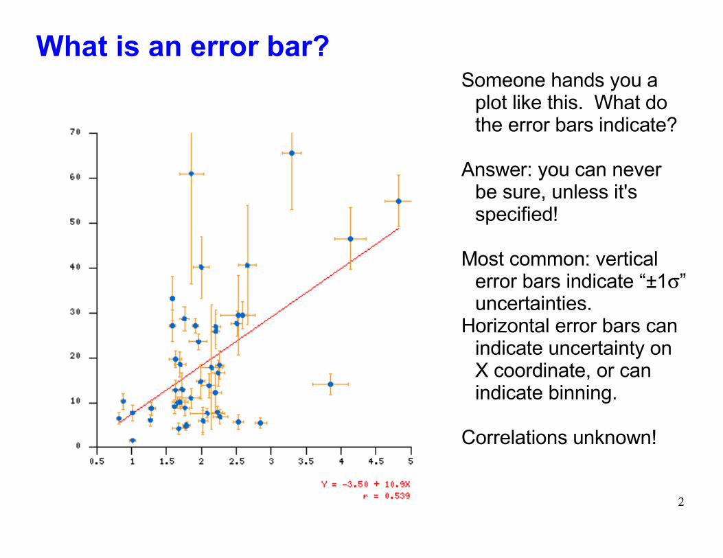
Physics 509 2

What is an error bar?Someone hands you a

plot like this. What do the error bars indicate?

Answer: you can never be sure, unless it's specified!

Most common: vertical error bars indicate �±1σ� uncertainties.

Horizontal error bars can indicate uncertainty on X coordinate, or can indicate binning.

Correlations unknown!

Physics 509 3

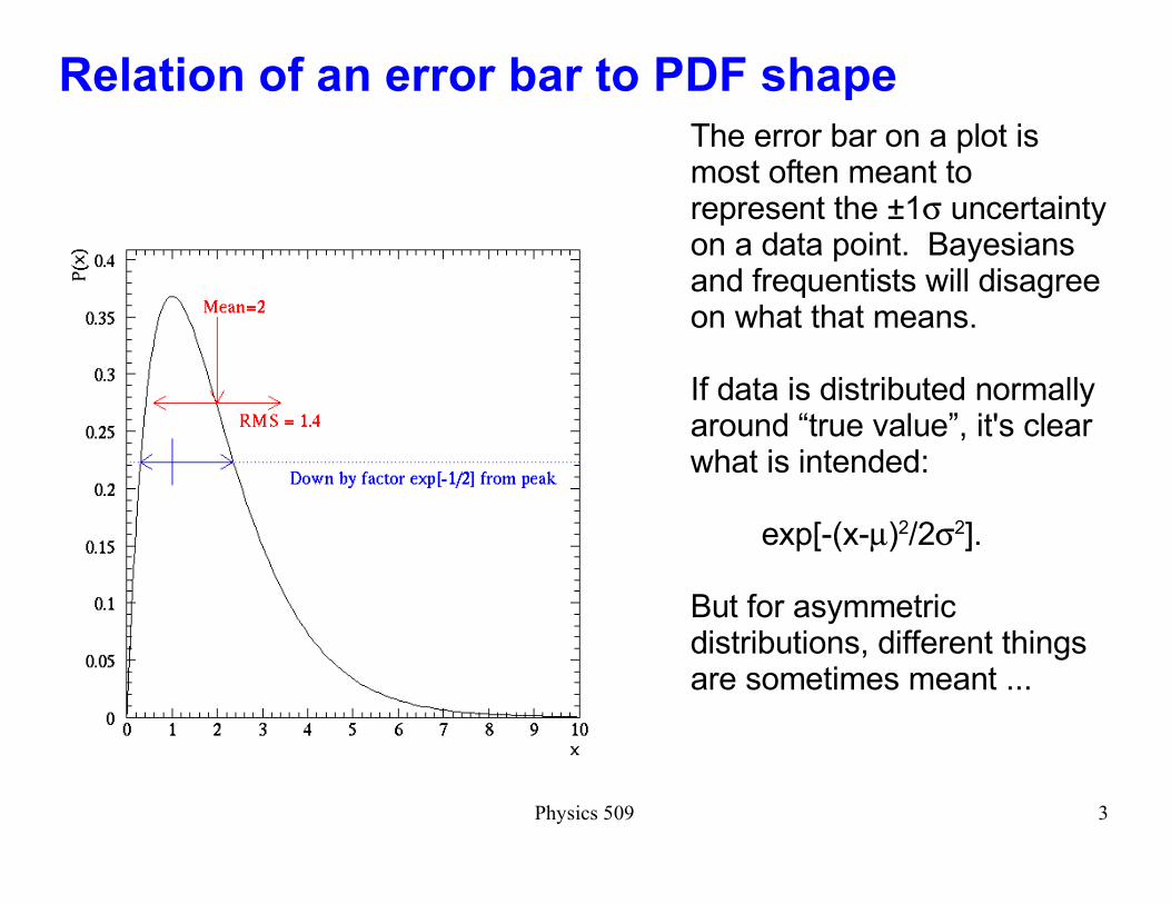
Relation of an error bar to PDF shape

The error bar on a plot is most often meant to represent the ±1σ uncertainty on a data point. Bayesians and frequentists will disagree on what that means.

If data is distributed normally around �true value�, it's clear what is intended: exp[-(x-µ)2/2σ2].

But for asymmetric distributions, different things are sometimes meant ...

Physics 509 4

An error bar is a shorthand approximation to a PDF!

In an ideal Bayesian universe, error bars don't exist. Instead, everyone will use the full prior PDF and the data to calculate the posterior PDF, and then report the shape of that PDF (preferably as a graph or table).

An error bar is really a shorthand way to parameterize a PDF. Most often this means pretending the PDF is Gaussian and reporting its mean and RMS.

Many sins with error bars come from assuming Gaussian distributions when there aren't any.

Physics 509 5

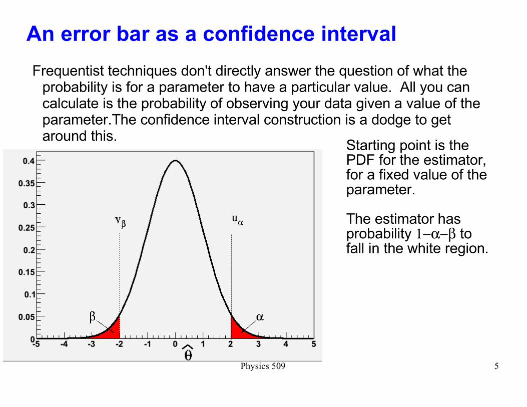
An error bar as a confidence interval

Frequentist techniques don't directly answer the question of what the probability is for a parameter to have a particular value. All you can calculate is the probability of observing your data given a value of the parameter.The confidence interval construction is a dodge to get around this.

Starting point is the PDF for the estimator, for a fixed value of the parameter.

The estimator has probability 1−α−β to fall in the white region.

Physics 509 7

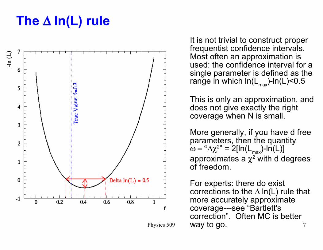
The ∆ ln(L) rule

It is not trivial to construct proper frequentist confidence intervals. Most often an approximation is used: the confidence interval for a single parameter is defined as the range in which ln(L

max)-ln(L)<0.5

This is only an approximation, and does not give exactly the right coverage when N is small.

More generally, if you have d free parameters, then the quantity

�ω = ∆χ2� = 2[ln(Lmax

)-ln(L)]

approximates a χ2 with d degrees of freedom.

For experts: there do exist corrections to the ∆ ln(L) rule that more accurately approximate coverage---see �Bartlett's correction�. Often MC is better way to go.

Physics 509 8

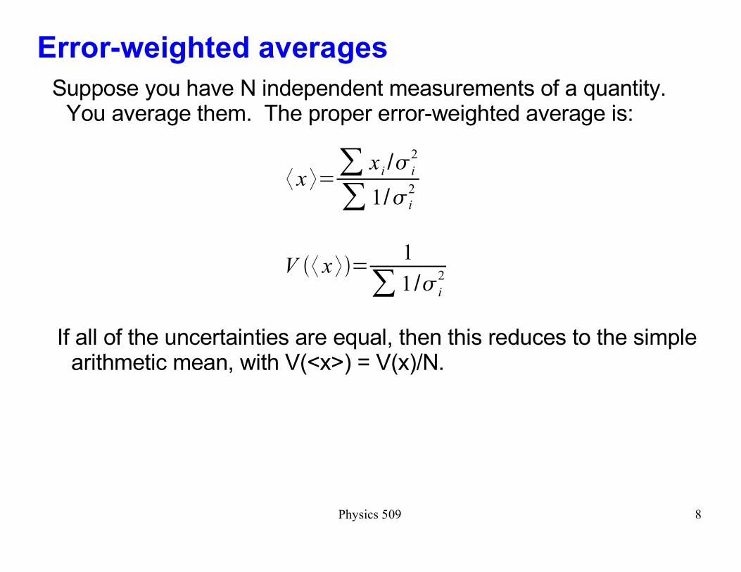
Error-weighted averages

Suppose you have N independent measurements of a quantity. You average them. The proper error-weighted average is:

� x �=� xi /� i

2

� 1/� i

2

V �� x ��=1

� 1 /� i

2

If all of the uncertainties are equal, then this reduces to the simple arithmetic mean, with V(<x>) = V(x)/N.

Physics 509 11

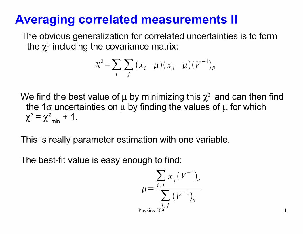
Averaging correlated measurements II

The obvious generalization for correlated uncertainties is to form the χ2 including the covariance matrix:

�2=�

i

�j

�xi����x j����V�1�ij

We find the best value of µ by minimizing this χ2 and can then find the 1σ uncertainties on µ by finding the values of µ for which

χ2 = χ2min

+ 1.

This is really parameter estimation with one variable.

The best-fit value is easy enough to find:

�=�i , j

x j �V�1�ij

�i , j

�V�1�ij

Physics 509 12

Averaging correlated measurements III

Recognizing that the χ2 really just is the argument of an exponential defining a Gaussian PDF for µ ...

�2=�

i

�j

�xi����x j����V�1�ij

we can in fact read off the coefficient of µ2, which will be 1/V(µ):

��2=

1

�i , j

�V�1�ij

In general this can only be computed by inverting the matrix as far as I know.

Physics 509 17

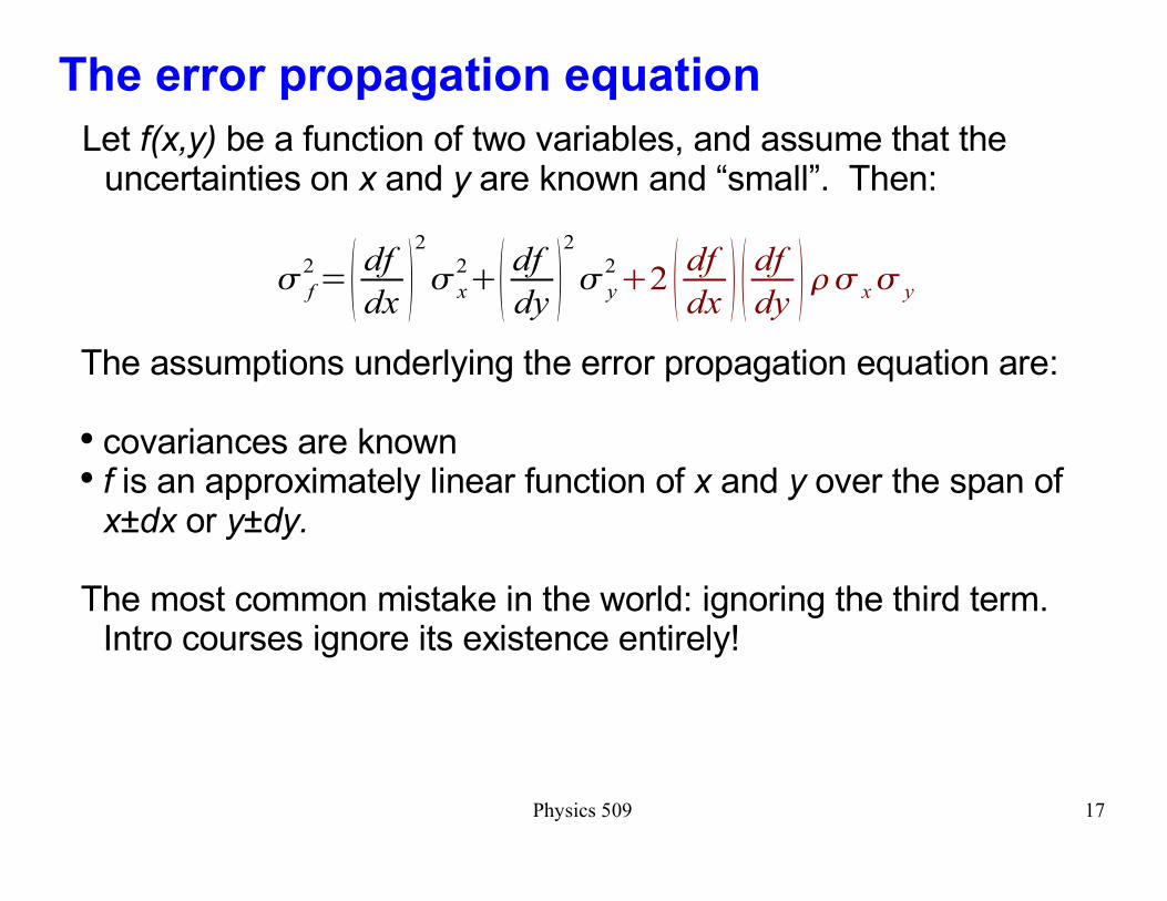
The error propagation equation

Let f(x,y) be a function of two variables, and assume that the uncertainties on x and y are known and �small�. Then:

� f

2= � dfdx �

2

� x

2�� dfdy �2

� y

2�2 � dfdx � � dfdy � �� x� y

The assumptions underlying the error propagation equation are:

� covariances are known� f is an approximately linear function of x and y over the span of

x±dx or y±dy.

The most common mistake in the world: ignoring the third term. Intro courses ignore its existence entirely!

Physics 509 18

Example: interpolating a straight line fit

Straight line fit y=mx+b

Reported values from a standard fitting package:

m = 0.658 ± 0.056b = 6.81 ± 2.57

Estimate the value and uncertainty of y when x=45.5:

y=0.658*45.5+6.81=36.75

UGH! NONSENSE!

dy=�2.572��45.5�.056�2=3.62

Physics 509 19

Example: straight line fit, done correctly

Here's the correct way to estimate y at x=45.5. First, I find a better fitter, which reports the actual covariance matrix of the fit:

m = 0.0658 + .056 b = 6.81 + 2.57 ρ = -0.9981

dy=�2.572��0.056�45.5�2�2 ��0.9981��0.056�45.5��2.57�=0.16

(Since the uncertainty on each individual data point was 0.5, and the fitting procedure effectively averages out their fluctuations, then we expect that we could predict the value of y in the meat of the distribution to better than 0.5.)

Food for thought: if the correlations matter so much, why don't most fitting programs report them routinely???

Physics 509 20

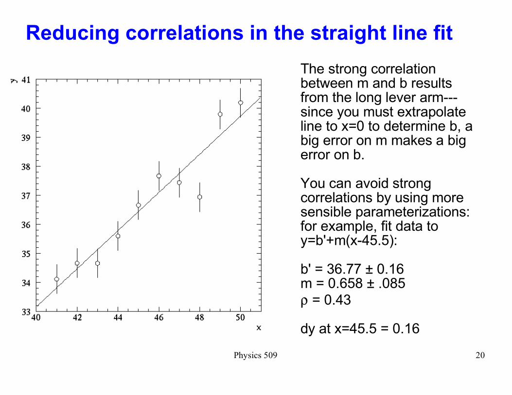
Reducing correlations in the straight line fit

The strong correlation between m and b results from the long lever arm---since you must extrapolate line to x=0 to determine b, a big error on m makes a big error on b.

You can avoid strong correlations by using more sensible parameterizations: for example, fit data toy=b'+m(x-45.5):

b' = 36.77 ± 0.16m = 0.658 ± .085

ρ = 0.43

dy at x=45.5 = 0.16