This article was downloaded by: [LIU Libraries]On: 25 January 2014, At: 10:03Publisher: RoutledgeInforma Ltd Registered in England and Wales Registered Number: 1072954 Registeredoffice: Mortimer House, 37-41 Mortimer Street, London W1T 3JH, UK

The Journal of Economic EducationPublication details, including instructions for authors andsubscription information:http://www.tandfonline.com/loi/vece20

A Simple Treatment of the LiquidityTrap for Intermediate MacroeconomicsCoursesSebastien Buttet a & Udayan Roy aa New York Institute of Technology-Old Westburyb Long Island University PostPublished online: 24 Jan 2014.

To cite this article: Sebastien Buttet & Udayan Roy (2014) A Simple Treatment of the Liquidity Trapfor Intermediate Macroeconomics Courses, The Journal of Economic Education, 45:1, 36-55, DOI:10.1080/00220485.2014.859959

To link to this article: http://dx.doi.org/10.1080/00220485.2014.859959

PLEASE SCROLL DOWN FOR ARTICLE

Taylor & Francis makes every effort to ensure the accuracy of all the information (the“Content”) contained in the publications on our platform. However, Taylor & Francis,our agents, and our licensors make no representations or warranties whatsoever as tothe accuracy, completeness, or suitability for any purpose of the Content. Any opinionsand views expressed in this publication are the opinions and views of the authors,and are not the views of or endorsed by Taylor & Francis. The accuracy of the Contentshould not be relied upon and should be independently verified with primary sourcesof information. Taylor and Francis shall not be liable for any losses, actions, claims,proceedings, demands, costs, expenses, damages, and other liabilities whatsoever orhowsoever caused arising directly or indirectly in connection with, in relation to or arisingout of the use of the Content.

This article may be used for research, teaching, and private study purposes. Anysubstantial or systematic reproduction, redistribution, reselling, loan, sub-licensing,systematic supply, or distribution in any form to anyone is expressly forbidden. Terms &Conditions of access and use can be found at http://www.tandfonline.com/page/terms-and-conditions

THE JOURNAL OF ECONOMIC EDUCATION, 45(1), 36–55, 2014Copyright C© Taylor & Francis Group, LLCISSN: 0022-0485 print/2152-4068 onlineDOI: 10.1080/00220485.2014.859959

CONTENT ARTICLE IN ECONOMICS

A Simple Treatment of the Liquidity Trap for IntermediateMacroeconomics Courses

Sebastien Buttet and Udayan Roy

Several leading undergraduate intermediate macroeconomics textbooks now include a simplereduced-form New Keynesian model of short-run dynamics (alongside the IS-LM model). Unfor-tunately, there is no accompanying description of how the zero lower bound on nominal interestrates affects the model. In this article, the authors show how the aforementioned model can easily bemodified to teach undergraduate students about the significance of the zero lower bound for economicperformance and policy. This acquires additional significance because economies such as the UnitedStates and Japan have been close to the zero lower bound since 2008 and 1995, respectively. Theauthors show that when the zero lower bound is introduced, an additional long-run equilibrium exists.This equilibrium is unstable and can lead to a deflationary spiral.

Keywords fiscal policy, intermediate macroeconomics, monetary policy, zero lower bound

JEL codes E12, E52, E62

The Great Recession of 2008–9 has changed the practice and teaching of macroeconomics.Authors of prominent textbooks have added entire chapters on the crisis and its aftermath in theirnew editions. The economy-wide ripples of developments in the financial sector have receivedconsiderable coverage. The zero lower bound (ZLB) on nominal interest rates is no longer ignoredor treated as a curiosity. In this article, we demonstrate a simple way to improve the integrationof the ZLB into the discussion of short-run macroeconomic theory and policy in undergraduatemacroeconomics textbooks.

Even a quick look at recent editions of prominent undergraduate macroeconomics textbookssuch as Mankiw (2013) or Jones (2011) shows that the IS-LM model is being supplemented bya reduced-form New Keynesian model consisting of the IS curve, the expectations-augmentedPhillips curve, and a monetary policy rule for the central bank. Unfortunately, in these textbook

Sebastien Buttet (e-mail: sbuttet@nyit.edu) is a scholar in residence at the New York Institute of Technology-OldWestbury. Udayan Roy (e-mail: udayan.roy@liu.edu) is a professor of economics at Long Island University Post. Buttetis the corresponding author.

Dow

nloa

ded

by [

LIU

Lib

rari

es]

at 1

0:03

25

Janu

ary

2014

LIQUIDITY TRAP IN INTERMEDIATE MACROECONOMICS 37

discussions, the central bank’s monetary policy rule simply ignores the ZLB; it is often mentioned,but it is not built into the theory. This will not do in a world in which the central banks of theUnited States and Japan have kept their policy rates near zero since 2008 and 1995, respectively.Bright and curious students will inevitably ask their instructors how the graphs of the NewKeynesian model that they have been taught would look when the central bank is at the ZLB. Inthis article, we show that the integration of the ZLB into the New Keynesian model is remarkablystraightforward and can yield interesting insights into, for instance, the dreaded phenomenon ofthe deflationary spiral.

In several of today’s undergraduate macroeconomics textbooks, the dynamic properties of NewKeynesian models are analyzed with two curves—a negatively sloped aggregate demand curveand a positively sloped aggregate supply curve—that link inflation and output. The intersectionof these two curves determines equilibrium output and inflation. We add the explicit requirementthat the nominal interest rate set by the central bank must be non-negative. We show that thefamiliar negatively sloped aggregate demand curve becomes a kinked curve with a negativelysloped segment (when the ZLB is nonbinding) and a positively sloped segment (when the ZLBis binding). The positively sloped segment captures the idea that falling inflation is a specialnightmare at the ZLB. As nominal interest rates cannot be reduced any further, any decline ininflation means an increase in the real interest rate which in turn reduces aggregate demand andoutput.

The kinked demand curve generates two (rather than one) long-run equilibria: (1) a stableequilibrium where nominal interest rates are positive and inflation is equal to the central bank’starget rate of inflation and (2) an unstable equilibrium at which the nominal interest rate is zeroand even the slightest shock can set off a deflationary spiral.

We show that the convergence properties of the economy depend on whether or not inflation isless than a tipping-point rate. As long as the inflation rate exceeds the negative of the natural (orlong-run) real interest rate, the economy converges to the stable long-run equilibrium—even ifthe ZLB is initially binding. On the other hand, if inflation falls below the negative of the naturalreal interest rate, the economy enters a deflationary spiral with continuously falling inflation andoutput.

With regard to the effectiveness of monetary and fiscal policy in dealing with the deflationaryspiral, we ask two questions: (1) What can be done to keep an economy away from the deflationaryspiral? and (2) Can policy get an economy out of a deflationary spiral if it is already in one? Weshow that expansionary fiscal policy is an adequate answer to both questions, while expansionarymonetary policy—specifically, an increase in the target inflation rate—is a partial answer to (1)only.

The main ideas within our article—(1) that the ZLB introduces a new long-run equilibrium;(2) that that equilibrium is unstable; (3) that the ZLB introduces a deflationary spiral; and (4)that there is a tipping point beyond which deflation leads to the deflationary spiral—have beenexplained here in the graphical form of chapter 15 in Mankiw (2013). All that an instructor whoteaches that chapter would have to do is show (a) that the central bank’s monetary policy ruledoes not always yield a positive nominal interest rate, and (b) that when the monetary policyrule yields a negative nominal interest rate, the ZLB kicks in and the aggregate demand curvebecomes positively sloped. Our four main results then immediately follow.

It is clear to us that unless the investment required—from both teacher and student—for adiscussion of the ZLB is kept low, our treatment of the ZLB would be unlikely to be useful in

Dow

nloa

ded

by [

LIU

Lib

rari

es]

at 1

0:03

25

Janu

ary

2014

38 BUTTET AND ROY

the classroom. This is why we have expressed our analysis in the graphical style of Mankiw’schapter 15. We have shown that the main results that follow from the introduction of the ZLBcan be taught to undergraduates with a simple change to Mankiw’s (dynamic) aggregate demandcurve. We believe that use of our article’s contents sharply reduces the marginal cost of teachingthe ZLB. Also, given that the ZLB yields several interesting results, the marginal benefit ofteaching Mankiw’s chapter 15 (or its counterpart in other textbooks) may now be higher for thoseinstructors who currently skip the chapter.

Although our analysis builds on Mankiw (2013), to make our analysis relevant and useful forinstructors who do not use that textbook, our penultimate section reviews the treatment of theZLB in five other prominent intermediate macroeconomics textbooks: Blanchard and Johnson(2013), Carlin and Soskice (2006), Jones (2011), Gordon (2012), and Mishkin (2011). Severalof these textbook authors present algebraic-cum-graphical models in which the intersection of(aggregate) demand and supply curves determine output and inflation. However, none of themshow how the ZLB affects their graphs. We explain how instructors who teach the New Keynesianmodel can modify their graphs and teach the ZLB with minimal hassle.

The remainder of the article is organized as follows: In the next two sections, we introduce ourmodel and characterize its long-run equilibria. We discuss the stability of these equilibria in ourfourth section, and we study policy responses to a deflationary environment in our fifth section.We discuss the treatment of the ZLB in several notable intermediate macroeconomics textbooksin our penultimate section. We offer brief concluding remarks in our last section.

A MODEL OF SHORT-RUN MACROECONOMIC DYNAMICS

Our goal here is to take a typical model of short-run macroeconomic dynamics from a standardundergraduate intermediate macroeconomics textbook and demonstrate how the analysis can beenriched if a non-negativity constraint on the nominal interest rate is added. The model that wehave chosen to use is variously referred to as the dynamic AD-AS (or DAD-DAS) model inMankiw (2013, ch. 15), the AS/AD model in Jones (2011), and the three-equation (IS-PC-MR)model in Carlin and Soskice (2006), where PC refers to the Phillips curve and MR refers tothe central bank’s monetary policy rule. This dynamic model has begun to supplement the staticIS-LM model as the mainstay of short-run analysis in undergraduate macroeconomics textbooks.It is our belief that adding the ZLB to the teaching of short-run macroeconomic dynamics inundergraduate courses will increase the realism and relevance of the analysis because the interestrates used by central banks as their instruments of monetary policy have been close to zero fora long time in several countries. For example, the bank rate of the Bank of England has been at0.5 percent since 2009. The federal funds rate, which is the policy rate for the Federal Reserve inthe United States, has been near zero since October 2008. The official discount rate in Japan hasbeen close to zero since 1995.

For specificity, we look at how the ZLB affects the DAD-DAS model in Mankiw (2013, ch. 15).We begin by examinimg the five equations that drive Mankiw’s DAD-DAS model. Equilibriumin the market for goods and services is given by

Yt = Yt − α · (rt − ρ) + εt (1)

Dow

nloa

ded

by [

LIU

Lib

rari

es]

at 1

0:03

25

Janu

ary

2014

LIQUIDITY TRAP IN INTERMEDIATE MACROECONOMICS 39

where Yt is real output at time t, Y t is the natural or long-run level of output, rt is the realinterest rate, ρ is the natural or long-run real interest rate, α is a positive parameter representingthe responsiveness of aggregate expenditure to the real interest rate, and εt represents demandshocks.1 This equation is essentially the well-known IS curve of the IS-LM model, and it hasno intertemporal dynamics. The shock εt represents exogenous shifts in demand that arise fromchanges in consumer and/or business sentiment—the so-called “animal spirits”—as well aschanges in fiscal policy. When the government implements a fiscal stimulus (an increase ingovernment expenditure or a decrease in taxes), εt is positive, whereas fiscal austerity makes εt

negative.The ex ante real interest rate in period t is determined by the Fisher equation (1933) and is

equal to the nominal interest rate it minus the inflation expected currently for the next period:

rt = it − Etπt+1. (2)

Inflation in the current period, π t, is determined by a conventional Phillips curve augmented toinclude the role of expected inflation, Et−1π t, and exogenous supply shocks, ν t:

πt = Et−1πt + φ · (Yt − Yt

) + νt (3)

where φ is a positive parameter.Inflation expectations play a key role in both the Fisher equation (2) and the Phillips curve (3).

As in Mankiw, we assume that inflation in the current period is the best forecast for inflation inthe next period. That is, agents have adaptive expectations:

Etπt+1 = πt . (4)

We complete the description of the DAD-DAS model with a monetary policy rule. DynamicNew Keynesian models assume that the central bank sets a target for the nominal interest rate, it,based on the inflation gap and the output gap, as in the Taylor rule (Taylor 1993). Specifically,the DAD-DAS model in Mankiw assumes that the monetary policy rule is it = π t + ρ + θπ ·(π t

– π∗) + θY·(Yt − Y t), where the central bank’s inflation target (π∗) and its policy parametersθπ and θY are all non-negative. We, however, wish to explicitly incorporate the fact that nominalinterest rates must be non-negative. Therefore, our generalized monetary policy rule is

it = max{0, πt + ρ + θπ · (

πt − π∗) + θY · (Yt − Yt

)}. (5)

Equations (1) through (5) describe our DAD-DAS model. For given values of the model’speriod-t parameters (α, ρ, φ, θπ , θY, π∗, and Y t), its period-t shocks (εt and ν t), and thepredetermined inflation rate (Et−1π t = π t−1) for period t−1, one can use the model’s fiveequations to solve for its five period-t endogenous variables (Yt, rt, it, Etπ t+1, and π t). Once it isunderstood that the inherited inflation rate (π t−1, which is also the previous period’s equilibriuminflation rate) determines the current equilibrium inflation rate, one sees the dynamics that areinternal to the DAD-DAS model. Parameter changes and/or shocks are not the only source ofchange; what happened yesterday determines what happens today which determines what happenstomorrow, and so on.2

For the graphical treatment of the model, we will—following Mankiw—turn our five equationsthat contain five endogenous variables into two equations that contain two endogenous variables,Yt and π t. The two equations will then be graphed as the dynamic aggregate demand (DAD) and

Dow

nloa

ded

by [

LIU

Lib

rari

es]

at 1

0:03

25

Janu

ary

2014

40 BUTTET AND ROY

dynamic aggregate supply (DAS) curves, with Yt on the horizontal axis and π t on the verticalaxis. The intersection of the two curves will determine the equilibrium values of Yt and π t.

The Kinked DAD Curve

Here, we introduce the only element of the DAD-DAS model of Mankiw that changes when theZLB on the nominal interest rate is added. To give away the punchline, Mankiw’s negativelysloped DAD curve becomes a kinked DAD curve with a negatively sloped segment (when theZLB is nonbinding) and a positively sloped segment (when the ZLB is binding).

Figure 1 shows, among other things, the border that separates the (Yt, π t) outcomes for whichthe ZLB is not binding from the (Yt, π t) outcomes for which the ZLB is binding. Algebraically,the monetary policy rule (5) implies that this border satisfies

πt + ρ + θπ · (πt − π∗) + θY · (

Yt − Yt

) = 0. (6)

Above this border, the ZLB is not binding and the nominal interest rate set by the central bank ispositive (it > 0); Mankiw’s analysis applies to this case word for word. On the border, the centralbank chooses a zero interest rate, but does so willingly, and not because it wanted a negative ratebut could not choose it because of the ZLB. Below the border, the ZLB is binding (it = 0).3

Mankiw derives the equation of his DAD curve as follows: Substitute adaptive expectations(4) and Mankiw’s simplified monetary policy rule [it = π t + ρ + θπ ·(π t – π∗) + θY·(Yt − Y t)]

FIGURE 1 Kinked DAD curve is shown here. It is assumed that εt = 0 and Y t = Y for all t (color figure availableonline).

Dow

nloa

ded

by [

LIU

Lib

rari

es]

at 1

0:03

25

Janu

ary

2014

LIQUIDITY TRAP IN INTERMEDIATE MACROECONOMICS 41

into the Fisher equation (2), substitute the resulting expression for the real interest rate in the ISequation (1), and rearrange and collect the terms. In this way, Mankiw gets

Yt = Yt − αθπ

1 + αθY

(πt − π∗) + 1

1 + αθY

εt . (7)

This is graphed as the negatively sloped line in the section of figure 1 where the ZLB is notbinding; note that dπ t/dYt < 0 in equation (7).

The DAD curve in figure 1 assumes that the demand shock is absent (εt = 0). Consequently,π t = π∗ and Yt = Y t satisfies equation (7). This is point O in figure 1; it will play an importantrole in our discussion of the model’s equilibrium below.

Note that equation (7) implies that Mankiw’s DAD curve (i.e., the DAD curve when the ZLB isnot binding) shifts rightward under both expansionary monetary policy (π∗↑) and expansionaryfiscal policy (εt↑). This is shown in figures 2 and 3.

Repeating Mankiw’s procedure, but with it = 0, we get the DAD curve for the case in whichthe ZLB is binding:

Yt = Yt + α · (πt + ρ) + εt . (8)

Note that the slope is positive (dπ t/dYt = 1/α > 0), which is why the DAD curve in figure 1turns into a positively sloped line below the ZLB border. The familiar negatively sloped DAD

FIGURE 2 Expansionary fiscal policy shifts the kinked DAD curve right without moving the ZLB border (color figureavailable online).

Dow

nloa

ded

by [

LIU

Lib

rari

es]

at 1

0:03

25

Janu

ary

2014

42 BUTTET AND ROY

FIGURE 3 Expansionary monetary policy shifts the ZLB border and the part of the DAD above the ZLB border to theright. The part of the DAD below the ZLB border just gets extended (color figure available online).

curve we see in textbooks becomes a kinked curve when the analysis allows the ZLB to bebinding. Algebra aside, the positively sloped segment is meant to capture the idea that fallinginflation is a special nightmare at the ZLB. As it = 0, any decline in current inflation means anincrease in the current real interest rate: As rt = it − Etπ t+1 = 0 − π t = −π t, we get drt/dπ t

= −1 < 0. The rising real interest rate reduces aggregate demand and output, as the familiar IScurve (1) dictates.4

By contrast, when the ZLB is not binding, the negatively sloped DAD curve reflects a differentstory. Any decrease in inflation provokes the monetary policy rule (5) to reduce the nominalinterest rate even more, as dictated by the Taylor principle. As a result, the real interest rate falls,thereby causing both aggregate demand and output to increase.

To finish our discussion of the rising segment of the DAD curve, when εt = 0, note that π t =−ρ and Yt = Y t satisfy equation (8). This is point D in figure 1. Like point O, D too will play animportant role in our discussion of the model’s equilibrium.

Equation (8) also implies that the positively sloped segment of the DAD curve shifts rightwardunder expansionary fiscal policy (εt↑) and is extended but not shifted by expansionary monetarypolicy (π∗↑). This is shown in figures 2 and 3.

The DAS Curve

When adaptive expectations (4) is substituted into the Phillips curve (3), we get Mankiw’s DAScurve:

πt = πt−1 + φ · (Yt − Yt

) + νt . (9)

Dow

nloa

ded

by [

LIU

Lib

rari

es]

at 1

0:03

25

Janu

ary

2014

LIQUIDITY TRAP IN INTERMEDIATE MACROECONOMICS 43

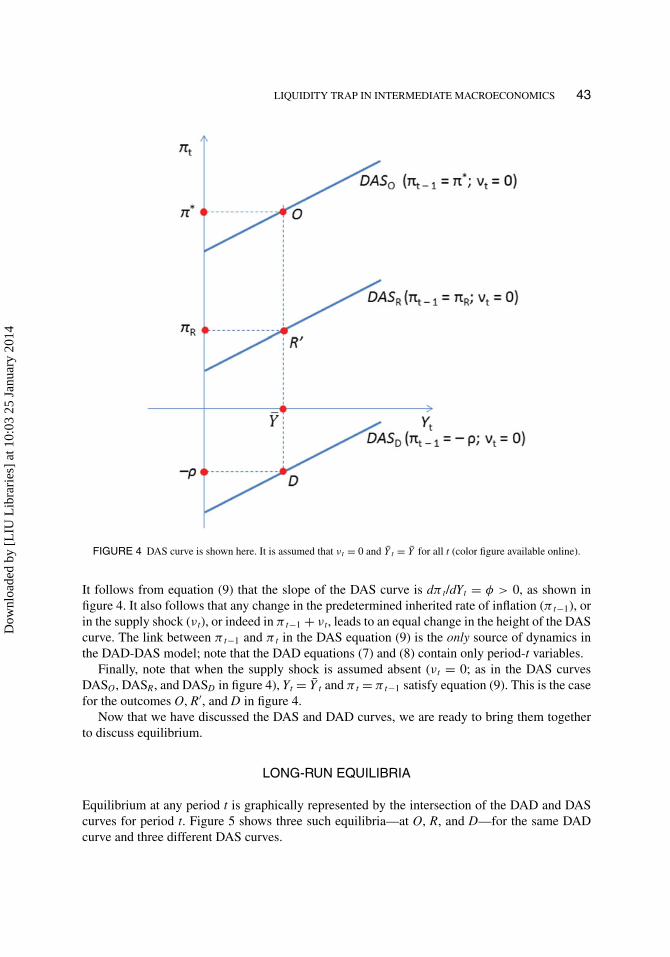
FIGURE 4 DAS curve is shown here. It is assumed that νt = 0 and Y t = Y for all t (color figure available online).

It follows from equation (9) that the slope of the DAS curve is dπ t/dYt = φ > 0, as shown infigure 4. It also follows that any change in the predetermined inherited rate of inflation (π t−1), orin the supply shock (ν t), or indeed in π t−1 + ν t, leads to an equal change in the height of the DAScurve. The link between π t−1 and π t in the DAS equation (9) is the only source of dynamics inthe DAD-DAS model; note that the DAD equations (7) and (8) contain only period-t variables.

Finally, note that when the supply shock is assumed absent (ν t = 0; as in the DAS curvesDASO, DASR, and DASD in figure 4), Yt = Y t and π t = π t−1 satisfy equation (9). This is the casefor the outcomes O, R′, and D in figure 4.

Now that we have discussed the DAS and DAD curves, we are ready to bring them togetherto discuss equilibrium.

LONG-RUN EQUILIBRIA

Equilibrium at any period t is graphically represented by the intersection of the DAD and DAScurves for period t. Figure 5 shows three such equilibria—at O, R, and D—for the same DADcurve and three different DAS curves.

Dow

nloa

ded

by [

LIU

Lib

rari

es]

at 1

0:03

25

Janu

ary

2014

44 BUTTET AND ROY

FIGURE 5 Both shocks are assumed zero, and Y t = Y for all t (color figure available online).

Let us begin with the equilibrium at R. As can be confirmed by a quick glance at the DASequation (9), as Yt > Y at R and as ν t = 0 has been assumed, it must be that π t > π t−1. Thatis, inflation is rising over time. Therefore, this is not what Mankiw calls a long-run equilibrium,which is an equilibrium outcome that repeats itself (as long as the model’s parameters stayunchanged and there are no shocks). As a general matter, if no restrictions are imposed on theDAD-DAS model’s parameters and shocks, there is no reason to expect an equilibrium outcometo repeat itself period after period. The question then is the following: Do there exist restrictionson the model’s parameters and shocks under which an equilibrium outcome would repeat itselfover and over again?

Let us now look at the equilibrium at O in figure 5. In this case, π t = π t−1 = π∗ and Yt =Y . With no parameter changes and no shocks, the DAD curve at t + 1 will be identical to theDAD curve at t, which is the one shown in figure 5. Also, as inherited inflation is the same inperiods t and t + 1 (π t−1 = π t = π∗) and ν t = ν t+1 = 0 by assumption, the DAS curve at t +1 will be identical to the DAS curve at t, which is DASO of figure 5. Therefore, O representsthe equilibrium outcome for periods t + 1 as well as t. In short, we have found an equilibriumthat repeats. We can conclude that (a) if the DAD-DAS model’s parameters stay constant, (b) ifthe two shocks stay at zero (εt = ν t = 0), and (c) if the inherited inflation happens to be equal

Dow

nloa

ded

by [

LIU

Lib

rari

es]

at 1

0:03

25

Janu

ary

2014

LIQUIDITY TRAP IN INTERMEDIATE MACROECONOMICS 45

to the central bank’s target inflation (π t−1 = π∗), then the equilibrium outcome will continueunchanged forever.

Mankiw goes on to show, algebraically and graphically, that the equilibrium at O in fig-ure 5—which we will henceforth refer to as the orthodox equilibrium—is the one and onlylong-run equilibrium of his DAD-DAS model (which, recall, makes no mention of the ZLB). Tofully describe the orthodox equlibrium, note that the monetary policy rule (5) implies it = π∗ +ρ, and the Fisher equation (2) and adaptive expectations (4) imply rt = it − Etπ t+1 = it − π t =ρ.

With the introduction of the ZLB, however, we now have a kinked DAD curve with a newpositively sloped segment, and it is straightforward to check that outcome D in figure 5, at theintersection of the kinked DAD curve and DASD, is also a long-run equilibrium. Although outputis Y and the real interest rate is ρ, exactly as in Mankiw’s orthodox equilibrium, the nominalinterest rate is zero—we are at the ZLB, after all—and the inflation rate is −ρ < 0. We call D thedeflationary equilibrium.

Before we move on to our discussion of the stability of our two long-run equilibria, a technicalissue must be discussed. Note that DASD in figure 5 is drawn flatter than the rising part of theDAD curve. This reflects our assumption that 1/α, which is the slope of the ZLB section of theDAD curve, exceeds φ, the slope of the DAS curve. Equivalently, we assume 1 − αφ > 0. Wediscuss this assumption further in a later section on the slopes of the DAD and DAS curves.

STABILITY OF LONG-RUN EQUILIBRIA

We will now show that not only does the ZLB add a new long-run equilibrium—the deflationaryequilibrium—to the DAD-DAS model, but also the deflationary equilibrium is unstable, unlikethe orthodox equilibrium, which is stable.

Let us assume that the parameters of the DAD-DAS model (α, ρ, φ, θπ , θY, π∗, and Y ) areconstant—and both shocks are at zero—from period t onwards. Under these conditions, we sawin our section on long-run equilibria that if π t−1 = π∗, the economy will stay at the othodoxequilibrium forever, and if π t−1 = −ρ, the economy will stay at the deflationary equilibriumforever. But what if π t−1 is neither π∗ nor −ρ? For arbitrary values of π t−1, how will the economybehave during periods t and later?

Under our assumption that the parameters (α, ρ, φ, θπ , θY, π∗, and Y ) are constant—and bothshocks are at zero—from period t onward, the kinked DAD curve will be the same for all periodst and later (as is clear from equations (7) and (8) in our section on the kinked demand curve). Letthis DAD curve be the one shown in figure 6.

Case 1: π t−1 > π∗. Let π t−1 = πQ > π∗. As π t−1 > π∗, the DAS curve at period t, indicatedin figure 6 by DASQ, must be higher than DASO, for which inherited inflation was specified to beπ t−1 = π∗. As we saw in our section on the DAS curve, the height of DASQ at Yt = Y is π t−1 =πQ > π∗, as shown in figure 6. The equilibrium at period t is, therefore, at q, with π t−1 > π t >

π∗. In other words, if inherited inflation exceeds π∗, current inflation will be lower than inheritedinflation while still remaining higher than π∗. Applying this result recursively while keeping inmind that this period’s current inflation is next period’s inherited inflation, we see that inflationconverges to π∗, and the equilibrium outcome converges to the orthodox equilibrium, O.5

Dow

nloa

ded

by [

LIU

Lib

rari

es]

at 1

0:03

25

Janu

ary

2014

46 BUTTET AND ROY

FIGURE 6 The orthodox equilibrium, O, is stable, and the deflationary equilibrium, D, is unstable. Y t = Y for all t(color figure available online).

Case 2: −ρ < π t−1 < π∗. Let −ρ < π t−1 = πR < π∗. Therefore, the DAS curve at t will besomewhere between DASO and DASD, for which inherited inflation was specified to be π t−1 = π∗

and π t−1 = −ρ, respectively. Let this DAS curve be DASR in figure 6. The period-t equilibriumis, therefore, at r with −ρ < π t−1 < π t < π∗. In other words, if inherited inflation lies between−ρ and π∗, current inflation will be higher than inherited inflation while still remaining between−ρ and π∗. Applying this result recursively while keeping in mind that this period’s currentinflation is next period’s inherited inflation, we see that the equilibrium outcome will converge tothe orthodox equilibrium, O.

Case 3: π t−1 < −ρ. Let π t−1 = πU < −ρ. The DAS curve at t will be below DASD. Let thisDAS curve be DASU in figure 6. The equilibrium will be at u with π t < π t−1 < −ρ. In otherwords, if inherited inflation is less than −ρ, current inflation will be lower than inherited inflationand therefore even farther below −ρ. Applying this result recursively while keeping in mindthat this period’s current inflation is next period’s inherited inflation, we see that the equilibrium

Dow

nloa

ded

by [

LIU

Lib

rari

es]

at 1

0:03

25

Janu

ary

2014

LIQUIDITY TRAP IN INTERMEDIATE MACROECONOMICS 47

outcome will diverge from the deflationary equilibrium, D, with both inflation and output fallingcontinuously. This is the much dreaded deflationary spiral.6

To sum up, we have shown that as long as the parameters of the DAD-DAS model do notchange and there are no shocks, the economy will either converge to the orthodox equilibriumor be in the ever-worsening deflationary spiral. The key knife’s edge factor is the inflation rate.If inflation falls below −ρ, which is the negative of the natural real interest rate, the economy’sfate is the deflationary spiral with ever-decreasing inflation and output. If the inflation rate staysabove −ρ, the economy converges to the orthodox long-run equilibrium at O, and there is noreason to worry.

Recall that in our discussion above we have assumed that φ, the slope of the DAS curve, issmaller than 1/α, the slope of the positively sloped segment of the DAD curve (under the ZLB).We will now argue that this assumption is necessary to avoid comparative static results that seemunrealistic to us.

Consider the equilibrium outcome a at the intersection of DAS and DAD1 in the left panel offigure 7. Note that contrary to our assumption above, DAS has been drawn steeper than DAD1.Now consider a positive demand shock (εt↑). As we saw in our section on the kinked DAD curveand figure 2, the economy’s DAD curve will shift rightward to, say, DAD1. Therefore, the newequilibrium will be at b. In other words, an increase in demand leads to lower inflation and loweroutput. This outcome strikes us as unrealistic.

Similarly, in the right panel of figure 7, we see another comparative static result that seemsunrealistic to us: an increase in the cost shock (ν t↑), such as increases in the price of importedoil or a series of bad droughts, leads to lower inflation.

These unrealistic comparative static results can be avoided by assuming 1/α > φ or, equiva-lently, 1−αφ > 0.

FIGURE 7 If DAS is steeper than DAD, a demand stimulus leads to lower output and lower inflation (left), and a supplyshock leads to lower inflation (right).

Dow

nloa

ded

by [

LIU

Lib

rari

es]

at 1

0:03

25

Janu

ary

2014

48 BUTTET AND ROY

POLICY RESPONSES TO DEFLATIONARY SPIRALS

Given that a deflationary spiral—with output decreasing without bound—is undesirable, (a) whatcan be done to keep an economy away from it, and (b) what can be done to get an economy out ofa deflationary spiral if it is already in one. We will show that expansionary fiscal policy—that is,an increase in εt in the goods market’s equilibrium condition (1)—is an adequate answer to bothquestions, and expansionary monetary policy—that is, an increase in the central bank’s targetinflation rate (π∗) in the monetary policy rule (5)—is a partial answer to (a).

Fiscal Stimulus Works

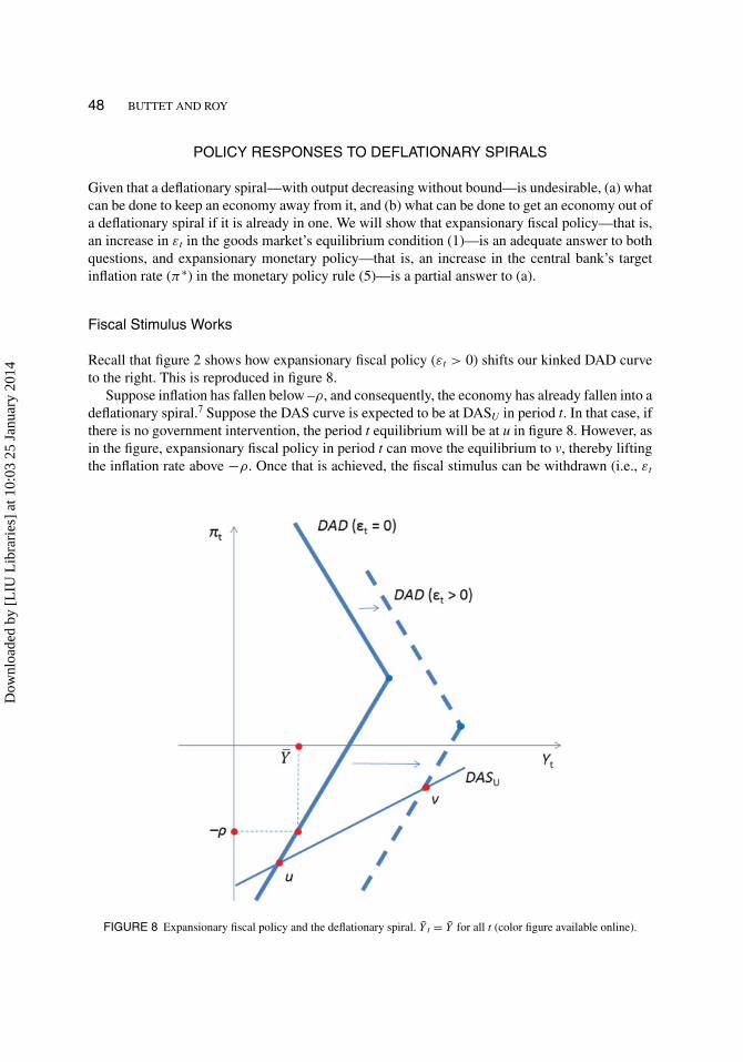
Recall that figure 2 shows how expansionary fiscal policy (εt > 0) shifts our kinked DAD curveto the right. This is reproduced in figure 8.

Suppose inflation has fallen below –ρ, and consequently, the economy has already fallen into adeflationary spiral.7 Suppose the DAS curve is expected to be at DASU in period t. In that case, ifthere is no government intervention, the period t equilibrium will be at u in figure 8. However, asin the figure, expansionary fiscal policy in period t can move the equilibrium to v, thereby liftingthe inflation rate above −ρ. Once that is achieved, the fiscal stimulus can be withdrawn (i.e., εt

FIGURE 8 Expansionary fiscal policy and the deflationary spiral. Y t = Y for all t (color figure available online).

Dow

nloa

ded

by [

LIU

Lib

rari

es]

at 1

0:03

25

Janu

ary

2014

LIQUIDITY TRAP IN INTERMEDIATE MACROECONOMICS 49

can return to zero and DAD can return to its original position), and as we have seen before, theeconomy will gradually converge to the orthodox equilibrium.

The same policy can also be used as a prophylactic. If, for some reason, it is imminent that theDAS curve will drop to DASU, we can use expansionary fiscal policy to shift the DAD curve tothe right, thereby nipping the deflationary spiral in the bud.

Finally, if inflation has been (or soon will be) pushed below −ρ by a leftward shift in theDAD curve (say, by a decline in “animal spirits” or “confidence”), then it goes without saying,expansionary fiscal policy can negate such a leftward shift.

Expansionary Monetary Policy May Work

Recall that figure 3 shows how expansionary monetary policy (π∗↑) shifts our kinked DAD curve.This is reproduced in figure 9.

Suppose the economy is at u in figure 9, inflation has dropped below −ρ, and therefore, adeflationary spiral is already underway. Expansionary monetary policy (which can only extendthe positively sloped segment of the DAD curve but not shift it) is of no use in this case. Adeflationary spiral can only occur when the ZLB on the nominal interest rate is binding. As aresult, monetary policy is ineffective in a deflationary spiral.

FIGURE 9 Expansionary monetary policy and the deflationary spiral. Both shocks are assumed zero. Y t = Y for all t(color figure available online).

Dow

nloa

ded

by [

LIU

Lib

rari

es]

at 1

0:03

25

Janu

ary

2014

50 BUTTET AND ROY

Similarly, if the ZLB is binding (say, the economy is at v in figure 9 on the positively slopedpart of the DAD curve), monetary policy would not be able to counteract an imminent decline inthe DAS curve to DASU that would initate a deflationary spiral.

However, suppose the economy is at x in figure 9, and an imminent decrease in the suplyshock is expected to take the economy to u. This threatens to reduce the inflation rate to −ρ

− δ and thereby initiate a deflationary spiral. In this case, because the ZLB is nonbinding at x,expansionary monetary policy (π∗↑) can raise the equilibrium inflation rate by , as a comparisonof points x and y shows. And if > δ, this would be enough to keep the equilibrium inflationrate above −ρ and thereby prevent a deflationary spiral.

To sum up, in the DAD-DAS model, expansionary fiscal policy can be used to rescue aneconomy that is already in a deflationary spiral and, preemptively, to stop an imminent deflationaryspiral. Expansionary monetary policy cannot help if a deflationary spiral is already underway. Itmay help to keep an economy out of a deflationary spiral, but only if the ZLB on the nominalinterest rate has not become binding.

THE ZLB IN PROMINENT TEXTBOOKS

We have shown how the graphical DAD-DAS model in Mankiw (2013) can be easily modifiedto include the ZLB on the nominal interest rate. We have also shown that the ZLB gives us adeflationary long-run equilibrium and a deflationary spiral. In this section, we will discuss thetreatment of these issues in five other intermediate macroeconomics textbooks: Blanchard andJohnson (2013), Carlin and Soskice (2006), Gordon (2012), Jones (2011), and Mishkin (2011).

These five textbooks all discuss the ZLB, and they all make the point that expansionary fiscalpolicy works at the ZLB whereas expansionary monetary policy (at least of the conventional kind)does not. The five equations of Mankiw’s DAD-DAS model—equations (1) through (5)—arepresent in all five textbooks. However, these five equations are scattered across multiple chaptersand are not analyzed together—either graphically or algebraically—as a unified model.

Using monetary policy rules that are somewhat different from Mankiw’s rule (5), Carlin andSoskice (2006), Jones (2011), and Mishkin (2011) present graphical models, which, like Mankiw,determine both output and inflation at the intersection of a negatively sloped demand curve anda positively sloped supply curve. Also, like Mankiw, they do not discuss how the ZLB affectstheir graphs. When we add the ZLB to the models in Carlin and Soskice, Jones, and Mishkin, weagain get kinked demand curves. For Carlin and Soskice and Jones, this kinked demand curvehas a positively sloped segment for inflation rates below a critical level, as in our modificationof Mankiw. For Mishkin, we again get a kink, but with a vertical segment instead of a positivelysloped segment.

Why the difference? In both Carlin and Soskice (2006) and Jones (2011), the Fisher equationand adaptive expectations yield the usual result that the current real interest rate equals the currentnominal interest rate less the current inflation rate: rt = it − π t. Therefore, at the ZLB, rt = −π t.As a result, lower current inflation leads to a higher current real interest rate, which, by the IScurve, leads to lower current output, thus yielding a positively sloped aggregate demand curvein (Y , π ) space. In Mishkin (2011), however, the Fisher equation is expressed as r = i – π e, andadaptive expectation is expressed as π e = π−1, which is inherited inflation. Therefore, the currentreal interest rate (r = i − π−1) is unaffected by current inflation (π ). Lower current inflation has

Dow

nloa

ded

by [

LIU

Lib

rari

es]

at 1

0:03

25

Janu

ary

2014

LIQUIDITY TRAP IN INTERMEDIATE MACROECONOMICS 51

no effect on current real interest rate and, therefore, no effect on current output, thus yielding avertical demand curve below the kink.

It seems natural to us to think that when the nominal interest rate is stuck at zero, lower inflationwill lead to higher real interest rates and, therefore, to lower output. However, this persuasive“story” of an economy at the ZLB does not follow from Mishkin’s treatment because of theseemingly minor difference in his treatment of the Fisher equation.

Although none of the five textbooks describe our deflationary long-run equilibrium, the text-books by Carlin and Soskice (2006) and Jones (2011) are distinctive because they providesomewhat informal but intuitive accounts of the deflationary spiral. They explain the deflationaryspiral as follows: Suppose ρ is the real interest rate consistent with full employment. If π < −ρ,then i = r + π ≥ 0 implies r ≥ −π > ρ. Therefore, as the actual real interest rate exceeds the realinterest rate consistent with full employment, full employment would not be possible. The result-ing recession would drive inflation farther below −ρ, and so on and on, causing a deflationaryspiral. While this explanation is intuitive, it is not complete (in our view) because current inflationis an endogenous variable, and it is simultaneously determined along with current output, thecurrent real interest rate, and the current nominal interest rate. It is necessary to explain why π <

−ρ would occur in the first place.Our analysis shows that if inherited inflation, which is a predetermined variable, reaches π t−1

< ρ, then a deflationary spiral occurs. To repeat, it is necessary to express the conditions that leadto a deflationary spiral entirely in terms of the model’s exogenous givens.

Both Blanchard and Johnson (2013) and Gordon (2012) present a graphical model that deter-mines current output and the current price level at the intersection of a negatively sloped demandcurve and a positively sloped supply curve. Unlike the other textbooks, Blanchard and Johnson(2013, 199, Fig. 9–10) also show how their demand curve looks under the ZLB: It is kinked, butwith a vertical, rather than positively sloped, segment for current inflation rates below a criticallevel at which the ZLB becomes binding. Blanchard and Johnson (2013, 296) also provide aninformal but valuable explanation of the deflationary spiral through an examination of the U.S.economy during the Great Depression.

In discussing the ZLB, Gordon (2012, 250) wrote the following:

In fact a falling price level increases the real interest rate (which is defined as the nominal interestrate minus the rate of inflation; when inflation is negative the real interest rate is higher than thenominal interest rate). A rising real interest rate caused by a falling price level reduces the demandfor interest-sensitive consumer durable goods and business investment in equipment and structuresand puts further downward pressure on real GDP.

However, a falling price level does not imply falling inflation.To summarize, although all six textbooks considered here take note of the ZLB, none describes

our deflationary long-run equilibrium, and none describes the conditions (in terms of the exoge-nous variables and parameters of the model economy) under which a deflationary spiral occurs.None of these textbooks describe how the ZLB changes the graphical determination of outputand inflation. We have tried to argue that a simple modification of the demand curve addressesall these issues.

Dow

nloa

ded

by [

LIU

Lib

rari

es]

at 1

0:03

25

Janu

ary

2014

52 BUTTET AND ROY

CONCLUSION

Several of today’s leading textbooks for intermediate macroeconomics courses include a dynamicNew Keynesian model of short-run macroeconomics consisting of an IS curve, a Phillips curve,and a monetary policy rule. We have shown in this article that when the DAD-DAS model inMankiw (2013) is generalized to incorporate the ZLB on the nominal interest rate, it has twolong-run equilibria, one stable and the other unstable. We have demonstrated the existence of adeflationary spiral in which both output and inflation fall without bound. We have also describedpolicy responses that can keep an economy out of the deflationary spiral and/or rescue it fromsuch a spiral in case one has already begun.

We realize that a deflationary spiral in which output falls without bound is unrealistic. InBlanchard and Johnson (2013, 178, “Deflation and the Philips Curve Relation”), the authorspoint out that during the Great Depression, inflation was systematically higher in the UnitedStates than predicted by the estimated (or fitted) Phillips curve. Based on this observation, theyargue persuasively that workers are reluctant to accept decreases in their nominal wages and thatthe Phillips curve relation breaks down at low levels of inflation. Adapting this article’s model todeal comprehensively with the deflationary spiral remains a topic for future research.

For the time being, note that monetary policy in the United States and Japan (to take just two ex-amples) has been stuck at the ZLB since 2008 and 1995, respectively. Students must see how short-run macroeconomics works under these no longer new—and no longer unusual—circumstances.

NOTES

1. For the graphical analysis in the rest of the article, we will make the simplifying assumption Yt = Y forall t.

2. While the algebra of these dynamics are worked out in the appendix, in the body of the article we presenta graphical treatment similar in style to that in a typical intermediate macroeconomics textbook.

3. Note from (6) that expansionary monetary policy (π∗↑) moves the ZLB border upward and to theright—thereby expanding the region where the ZLB is binding—whereas expansionary fiscal policy(εt↑) has no effect on the ZLB border.

4. The negative feedback loop between output and inflation is the mechanism that leads to a deflation-induced depression, as previously explained by Fisher (1933) and Krugman (1998). In normal times,when nominal interest rates are positive, the central bank can afford to cut interest rates following anegative demand shock to provide short-run stimulus to the economy. When the ZLB is binding, however,cutting rates is not feasible and real interest rates spike up as a result of lower inflation. Higher real ratesin turn depress the economy further, which put further pressure on real rates, which depress the economyfurther, and so on and so forth. As discussed in our section on textbooks, this idea is also explored inseveral textbooks, such as Gordon (2012).

5. Algebraic proofs of the stability results of this section are given in the appendix.6. Note that the good news of a favorable cost shock (ν t↓) (e.g., a fall in the price of imported oil) can

trigger a deflationary spiral by lowering the DAS curve, say, from DASD to DASU . This point has beenunderscored by Carlstrom and Pescatori (2009): “[T]o be effective in an environment of zero short-termnominal interest rates, monetary policy needs to be unequivocally committed to avoiding expectationsof deflation. . . . While this policy prescription follows from the assumption that the zero interest ratebound is a consequence of a negative demand shock hitting the economy, it is worth stressing that fallingprices can also be the consequence of a supply shock, namely particularly high productivity growth (nota bad thing!).”

7. See the discussion in our section on stability.

Dow

nloa

ded

by [

LIU

Lib

rari

es]

at 1

0:03

25

Janu

ary

2014

LIQUIDITY TRAP IN INTERMEDIATE MACROECONOMICS 53

ACKNOWLEDGEMENTS

The authors thank Professor Veronika Dolar for her helpful suggestions and comments.

REFERENCES

Blanchard, O., and D. R. Johnson. 2013. Macroeconomics. 6th ed. Upper Saddle River, NJ: Prentice Hall.Carlin, W., and D. Soskice. 2006. Macroeconomics: Imperfections, institutions, and policies. New York: Oxford University

Press.Carlstrom, C. T., and A. Pescatori. 2009. Conducting monetary policy when interest rates are near zero. http://www.

clevelandfed.org/research/commentary/2009/1009.cfm (accessed July 12, 2013).Fisher, I. 1933. The debt-deflation theory of great depressions. Econometrica 1(4): 337–57.Gordon, R. J. 2012. Macroeconomics. 12th ed. Upper Saddle River, NJ: Pearson Education.Jones, C. I. 2011. Macroeconomics. 2nd ed. New York: W. W. Norton.Krugman, P. 1998. It’s baack! Japan’s slump and the return of the liquidity trap. Brookings Papers on Economic Activity

29(2): 137–87.Mankiw, G. N. 2013. Macroeconomics. 8th ed. New York: Worth Publishers.Mishkin, F. S. 2011. Macroeconomics: Policy and practice. 1st ed. Upper Saddle River, NJ: Prentice Hall.Taylor, J. B. 1993. Discretion versus policy rules in practice. Carnegie-Rochester Conference Series on Public Policy 39:

195–214.

APPENDIX

AN ALGEBRAIC REPRESENTATION OF THE MODEL

Mankiw (2013, ch. 15) presents numerical simulations of the dynamic adjustment of the DAD-DAS model’s economy to various shocks and policy changes. These simulations require that theequilibrium values of the model’s endogenous variables be expressed in terms of the model’sparameters, shocks, and the predetermined value of inherited inflation. In this appendix, wecomplete this algebraic task.

When the ZLB is Not Binding

In this section, we assume that the ZLB is not binding. Later in this section, we will specify theconditions (in terms of the model’s parameters, shocks, and the predetermined value of inheritedinflation) under which the ZLB is not binding.

We have seen the derivation of the DAD curve (7) and the DAS curve (9). The former yields

Yt − Yt = − αθπ

1 + αθY

(πt − π∗) + 1

1 + αθY

εt .

By substituting this for Y t − Y t in (9), rearranging and collecting the terms, we get the short-runequilibrium inflation:

πt = (1 + αθY ) (πt−1 + νt ) + φ · (αθππ∗ + εt )

1 + αθY + αθπφ. (10)

Note that equation (10) is simulation-ready. By substituting numerical values for the model’sparameters, shocks, and the predetermined value of inherited inflation, we can calculate thenumerical value of the current period’s inflation. As this period’s current inflation is next period’s

Dow

nloa

ded

by [

LIU

Lib

rari

es]

at 1

0:03

25

Janu

ary

2014

54 BUTTET AND ROY

inherited inflation, the exercise can be repeated ad infinitum. Note also that current inflation isincreasing in inherited inflation, the cost shock, and the demand shock, as one would expect.

By substituting (10) into the DAD curve (7), we get the short-run equilibrium output:

Yt = Yt + αθπ · (π∗ − πt−1 − νt ) + εt

1 + α · (θπφ + θY ). (11)

Note that output increases under expansionary monetary policy (π∗↑) and/or expansionary fiscalpolicy (εt↑).

By substituting (11) into Mankiw’s simplified monetary policy rule [it = π t + ρ + θπ ·(π t –π∗) + θY·(Yt − Y t)], we get the short-run equilibrium nominal interest rate:

it = ρ + (1 + θπ + αθY ) (πt−1 + νt ) − (1 − αφ) θππ∗ + (θY + φ · (1 + θπ )) εt

1 + α · (θY + φθπ ). (12)

Equations (2) and (4) together imply that the real interest rate is rt = it − Etπ t+1 = it − π t.By substituting equations (10) and (12) into rt = it − π t, we get

rt = ρ + θπ · (πt−1 + νt − π∗) + (θY + θπφ) εt

1 + αθY + αθπφ. (13)

Equation (12) can now be used to derive the conditions under which the ZLB is binding or not.Let πc

t−1 be that rate of inherited inflation (π t−1) for which it = 0 in equation (12). By equatingthe righthand side of equation (12) to zero and rearranging the terms, we get the following:

πct−1 ≡ (1 − αφ) θππ∗ − (1 + αθY + αφθπ ) ρ − (θY + φ + φθπ ) εt

1 + αθY + θπ

− νt . (14)

We already know by definition that (a) it = 0 when π t−1 = πct−1. As equation (12) implies

that the nominal interest rate is strictly increasing in the inherited inflation rate ∂it/∂π t−1 > 0, itfollows further that (b) it > 0 when π t−1 > πc

t−1, and (c) it < 0 when π t−1 < πct−1. However, we

know from (5) that the nominal interest rate cannot be negative. Therefore, we conclude that theZLB is binding if and only if π t−1 < πc

t−1. Therefore, the expressions for inflation, output, andthe interest rates derived above are valid only when π t−1 ≥ πc

t−1.Returning to the equilibrium inflation rate (10) above, it can be checked that if εt = vt = 0

and π t−1 = π∗ are substituted in equation (10), we get π t−1 = π t = π∗. In other words, whenthere are no shocks, if the inherited inflation is equal to the central bank’s target inflation, then theinflation rate repeats itself ad infinitum. This is the orthodox long-run equilibrium of our sectionon long-run equilibria.

By substituting εt = vt = 0 and π t−1 = π t = π∗ into equations (11), (12), and (13) above, itis straightforward to show that in the orthodox long-run equilibrium, output is Y t, the nominalinterest rate is ρ + π∗, and the real interest rate is ρ.

The stability of the orthodox long-run equilibrium can now be proved. If we subtract π∗ fromboth sides of equation (10) and rearrange and collect the terms, we get, when there are no shocks(εt = vt = 0),

πt − π∗ = 1 + αθY

1 + αθY + αθπφ

(πt−1 − π∗) .

As 0 < (1 + αθY)/(1 + αθY + αθπ φ) < 1, it follows that the gap between inflation and the centralbank’s target inflation retains its sign and shrinks over time (as long as there are no shocks and the

Dow

nloa

ded

by [

LIU

Lib

rari

es]

at 1

0:03

25

Janu

ary

2014

LIQUIDITY TRAP IN INTERMEDIATE MACROECONOMICS 55

model’s parameters stay constant). In other words, if the ZLB is nonbinding (π t−1 ≥ πct−1), the in-

flation rate (π t) converges monotonically to the orthodox long-run equilibrium inflation rate (π∗).It is then straightforward, using equations (11), (12), and (13), that output and the interest rates

also converge to their respective orthodox long-run values.

When the ZLB is Binding

We now assume that the ZLB is binding (π t−1 < πct−1). In this case, the nominal interest rate set

by the central bank is it = 0. Easy!We have seen the derivation of the DAD curve (8) and the DAS curve (9). The former yields

Yt − Y t = α·(π t + ρ) + εt. By substituting this expression for Yt − Y t into (9), rearranging andcollecting the terms, we get the short-run equilibrium inflation rate:

πt = πt−1 + νt + αφρ + φεt

1 − αφ. (15)

Simulation-ready expressions for the real interest rate and output can be derived by substitutingequation (15) into rt = it − Etπ t+1 = it − π t = 0 − π t = −π t and (8).

It can be checked that if εt = vt = 0 and π t−1 = −ρ are substituted in equation (15), we getπ t−1 = π t = −ρ. In other words, when there are no shocks, if the inherited inflation happens to beequal to the negative of the natural (long-run) real interest rate, then that inflation rate repeats itselfad infinitum. This is the deflationary long-run equilibrium of our section on long-run equilibria.

The unstable nature of the deflationary long-run equilibrium can now be proved. If we subtract−ρ from both sides of equation (15) and rearrange and collect the terms, we get the following:

πt − (−ρ) = πt−1 − (−ρ) + νt + φεt

1 − αφ.

When there are no shocks (εt = vt = 0), this becomes

πt − (−ρ) = 1

1 − αφ· (πt−1 − (−ρ)) .

As we have assumed 0 < 1 − α φ < 1 (see our section on the slopes of the DAD and DAScurves), it follows that 1/(1 − α φ) > 1. Therefore, the gap between current equilibrium inflationand inflation in the deflationary long-run equilibrium retains its sign and increases—in absolutevalue—over time (as long as there are no shocks and the model’s parameters stay constant). Inother words, if the ZLB is binding (π t−1 < πc

t−1), the inflation rate (π t) diverges monotonicallyfrom the deflationary long-run equilibrium inflation rate (−ρ).

We can summarize our convergence results as follows:

Proposition 1: Assume there are no shocks. If π t−1 > −ρ, the economy converges to the orthodoxlong-run equilibrium. If π t−1 = −ρ, the economy stays in the deflationary long-run equilibrium. Ifπ t−1 < −ρ, the economy stays in a deflationary spiral.

Dow

nloa

ded

by [

LIU

Lib

rari

es]

at 1

0:03

25

Janu

ary

2014