Course Review for Final

ECE460Spring, 2012

2

Common Fourier Transform Pairs

Time Frequency 1 t 1

2 1 f

3 0t t 02j f te

4 02j f te 0f f

5

cos 2 of t 0 0

1

2f f f f

6 0sin 2 f t 0 02

jf f f f

7 t sinc f

8 t 2sinc f

9 2sinc t f

10 , 0te u t 1

2j f

11 , 0tt e u t 2

1

2j f

12 , 0te 22

2

2 f

13 2te 2fe

14 sgn t 1

j f

15 u t 1 1

2 2f

j f

16 ( )n t 2n

j f

17 1

t sgnj f

18 0j n tn

n

X e

02 n

n

X n

19 0n

t nT

0 0

1

n

nf

T T

( ) ( ) 2j f tx t X f e dfp¥

- ¥ò@ ( ) 2( ) j f tX f x t e dtp

¥-

- ¥ò@

3

Fourier Transform Properties

Property Time Frequency Linearity 1 1 2 2( ) ( )x t x t 1 1 2 2( ) ( )X f X f

Time Shift 0x t t 02j f te X f

Duality X t x f

Time Scaling x at 1 f

Xa a

Convolution x t y t X f Y f

Multiplication ( ) ( )x t y t ( ) ( )X f Y f

Parseval’s Theorem

*( )x t y t dt

*( )X f Y f df

Differentiation n

n

dx t

dt 2

nj f X f

Integration t

x d

( ) 1(0) ( )

2 2

X fX t

j f

Rayleigh’s 2x d

2

X f df

Autocorrelation *( )xR t x t x t d

2[ ( )]xR t X fF

Moments nt x d

02

n n

n f

j dX f

df

Modulation 0( ) cos(2 )x t f t 0 0

1 1( ) ( )

2 2X f f X f f

( ) ( ) 2j f tx t X f e dfp¥

- ¥ò@ ( ) 2( ) j f tX f x t e dtp

¥-

- ¥ò@

4

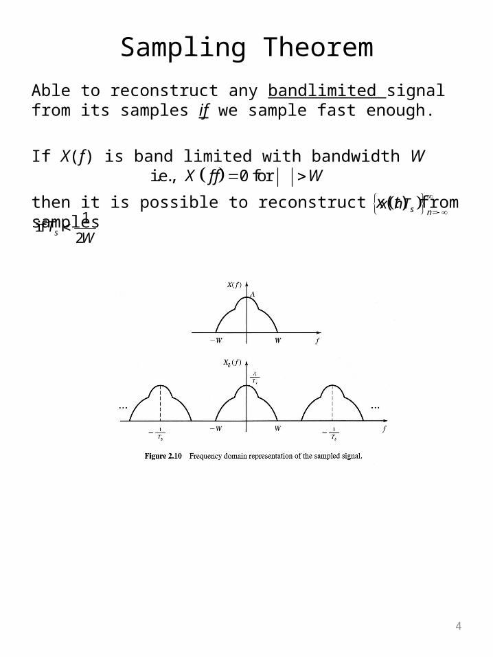
Sampling TheoremAble to reconstruct any bandlimited signal from its samples if we sample fast enough.

If X(f) is band limited with bandwidth W

then it is possible to reconstruct x(t) from samples i.e., 0 for X f f W

s nx nT

1if

2sTW

5

Bandpass Signals & SystemsFrequency Domain:

Low-pass Equivalents:

Let

Giving

To solve, work with low-pass parameters (easier mathematically), then switch back to bandpass via

Y f X f H f

0 0 02lY f u f f X f f H f f

0 0

0 0

2

2

l

l

X f u f f X f f

H f u f f H f f

1

21

2

l l l

l l l

Y f X f H f

y t x t h t

2Re oj f tly t y t e

6

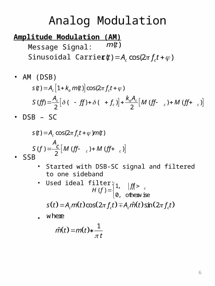
Analog ModulationAmplitude Modulation (AM)

Message Signal:Sinusoidal Carrier:

• AM (DSB)

• DSB – SC

• SSB• Started with DSB-SC signal and filtered to one sideband• Used ideal filter:

•

( )m t

( ) cos(2 )c cc t A f t

( ) 1 ( ) cos(2 )

( ) ( ) ( ) ( ) ( )2 2

c a c

c a cc c c c

s t A k m t f t

A k AS f f f f f M f f M f f

( ) cos(2 ) ( )

( ) ( ) ( )2

c c

c c

s t A f t m t

AcS f M f f M f f

1,( )

0, otherwisecf f

H f

ˆcos 2 sin 2

where

1ˆ

c c c cs t A m t f t A m t f t

m t m tt

7

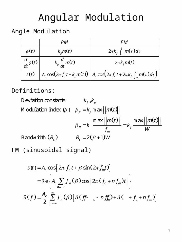
Angular ModulationAngle Modulation

Definitions:

FM (sinusoidal signal)

2

2

cos 2 cos 2 2

t

p f

p f

t

c c p c c f

PM FM

t k m t k m d

d dt k m t k m t

dt dt

s t A f t k m t A f t k m d

Deviation constants ,

Modulation Index ( ) max

max max

Bandwidth 2 1

f p

p p

f f fm

c c

k k

k m t

m t m tk k

f W

B B W

( ) cos 2 sin 2

Re cos 2

2

c c m

c n c mn

cn c m c m

n

s t A f t f t

A J f n f t

AS f J f f n f f f n f

8

Combinatorics1. Sampling with replacement and ordering

2. Sampling without replacement and with ordering

3. Sampling without replacement and without ordering

4. Sampling with replacement and without ordering

Bernoulli Trials

Conditional Probabilities

where = population size and = subpopulation sizern n r

!

!

n

n r

!

! !

n n

r n r r

1n r

r

probability of success and 1 probability of failure

A event of k-success in n-trialsk

p p

1

; , Binomial Law

n kkk

nP A p p

k

b k n p

1 2

21 2 2

, 0( | )

0, Otherwise

P E EP E

P E E P E

9

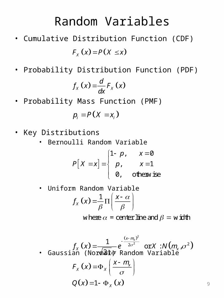
Random Variables• Cumulative Distribution Function (CDF)

• Probability Distribution Function (PDF)

• Probability Mass Function (PMF)

• Key Distributions• Bernoulli Random Variable

• Uniform Random Variable

• Gaussian (Normal) Random Variable

XF x P X x

X X

df x F x

dx

i ip P X x

1

where = center line and width

X

xf x

1 , 0

, 1

0, otherwise

p x

P X x p x

2

2 221 or : ,

2

1

xx m

X x

xX X

X

f x e X N m

x mF x

Q x x

10

Functions of a Random VariableGeneral:

Statistical Averages• Mean

• Variance

:

where number of g x equal to y

Y

X iY i

i i

Y g X

F y P g X y

f xf y i

g x

x Xm E X x f x dx

22x xE X m

11

Multiple Random VariablesJoint CDF of X and Y

Joint PDF of X and Y

Conditional PDF of X

Expected Values

Correlation of X and Y

Covariance of X and Y - what is ρX,Y?

Independence of X and Y

, , ,X YF x y P X x Y y

2

, , ,X Y XYf x y F x yx y

,, , ,X YE g X Y g x y f x y dx dy

,( , ) ( ( , )) ,XY X YR x y E g X Y x y f x y dx dy

,COV( , ) ( )( ) ,x y X YX Y x m y m f x y dx dy

,

|

,, 0

|

0, otherwise

X YX

Y X X

f x yf x

f y x f x

, ,X Y X Yf x y f x f y

Jointly Gaussian R.V.’sX and Y are jointly Gaussian if

Matrix Form:

Function:

12

, 221 2

2 2

1 2 1 22 21 2 1 2

1 1, exp

2 12 1

2

X Yf x y

x m y m x m y m

1 1 2 1

2 1 2 2

1

Var Cov , Cov ,

Cov , Var Cov ,

Cov , Var

covariance matrix of .

T

n

n

n n

E

X X X X X

X X X X X

X X X

C X m X m

X

1[ ]

mean vector of .

[ ]n

E X

E

E X

m X X

11

22

1 1exp

22

T

nf

X x x m C x mC

Y AX b

Y XE E m Y A X b Am b

T

Y Y Y

T TX X

TX

E

E

C Y m Y m

A X m X m A

AC A

13

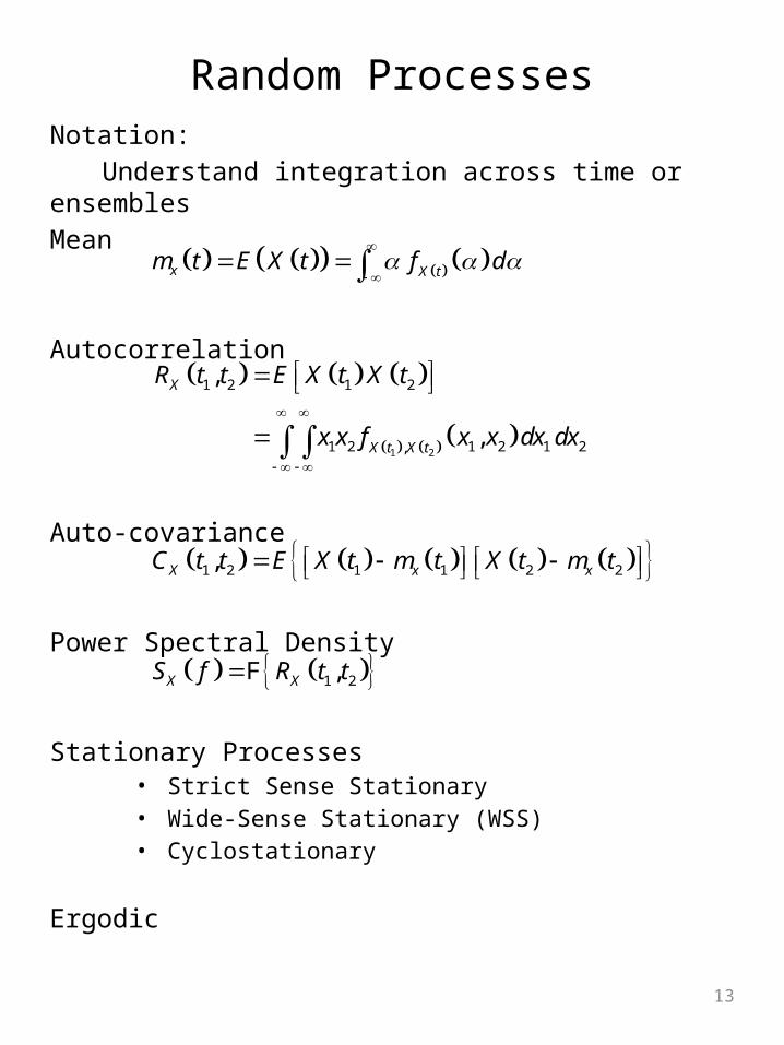
Random ProcessesNotation:

Understand integration across time or ensemblesMean

Autocorrelation

Auto-covariance

Power Spectral Density

Stationary Processes• Strict Sense Stationary• Wide-Sense Stationary (WSS)• Cyclostationary

Ergodic

x X tm t E X t f d

1 2

1 2 1 2

1 2 1 2 1 2,

,

,

X

X t X t

R t t E X t X t

x x f x x dx dx

1 2 1 1 2 2,X x xC t t E X t m t X t m t

1 2,X XS f R t tF

14

Transfer Through a Linear System

Mean of Y(t) where X(t) is wss

Cross-correlation function RXY(t1,t2)

Autocorrelation function RY(t1,t2)

Spectral Analysis

h t X t Y t

0Y X Xm t E Y t m h s ds m H

1 2 1 2,XY

X

R t t E X t Y t

R h

1 2 1 2,Y

XY

X

R t t E Y t Y t

R h

R h h

2

X X

XY XY X

Y X

S f R

S f R S f H f

S f S f H f

F

F

15

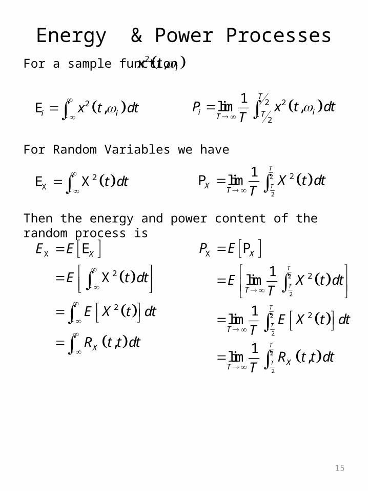
Energy & Power ProcessesFor a sample function

For Random Variables we have

Then the energy and power content of the random process is

2 ,i ix t dt

E

X

2

2

X

,

X

X

E E

E t dt

E X t dt

R t t dt

E

2 , ix t

2X X t dt

E

2 2

2

1lim ,

T

i iTTP x t dt

T

2

2

21lim

T

TX TX t dt

T P

2

2

2

2

2

2

X

2

2

1lim

1lim

1lim ,

T

T

T

T

T

T

X

T

T

XT

P E

E X t dtT

E X t dtT

R t t dtT

P

16

Zero-Mean White Gaussian NoiseA zero mean white Gaussian noise, W(t), is a random process with

4. For any n and any sequence t1, t2, …, tn the random variables W(t1), W(t2), …, W(tn), are jointly Gaussian with zero mean

and covariances

1. 0

2.2

3. Watt/Hz2

oW

oW

E W t t

NR E W t W t

NS f

, cov

(since zero mean)

2

X i j i j

i j

W j i

oj i

K t t W t W t

E W t W t

R t t

Nt t

0 for 1,2,...,iE W t i n

17

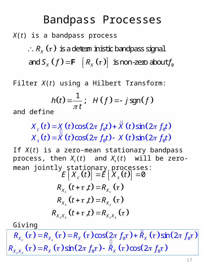
Bandpass ProcessesX(t) is a bandpass process

Filter X(t) using a Hilbert Transform:

and define

If X(t) is a zero-mean stationary bandpass process, then Xc(t) and Xs(t) will be zero-mean jointly stationary processes:

Giving

0

is a deterministic bandpass signal

and is non-zero about

X

X X

R

S f R f

F

1; sgnh t H f j f

t

0 0

0 0

cos 2 sin 2

cos 2 sin 2c

s

X t X t f t X t f t

X t X t f t X t f t

0

,

,

,

c c

s s

c s c s

c s

X X

X X

X X X X

E X t E X t

R t t R

R t t R

R t t R

0 0

0 0

cos 2 sin 2

sin 2 cos 2c s

c s

X X X X

X X X X

R R R f R f

R R f R f

18

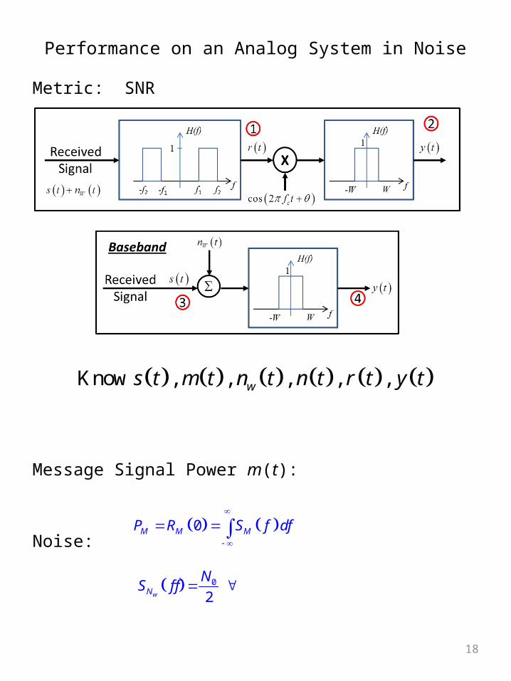
Performance on an Analog System in Noise

Metric: SNR

Message Signal Power m(t):

Noise: 0M M MP R S f df

0

2wN

NS f f

Know , , , , ,ws t m t n t n t r t y t

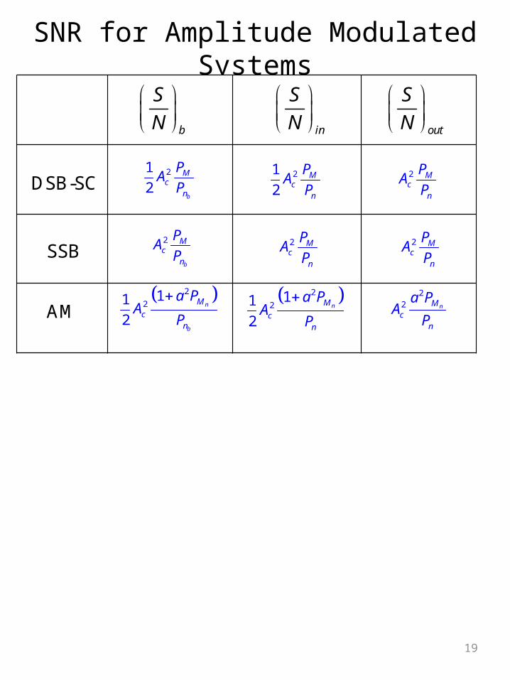
19

SNR for Amplitude Modulated Systems

b

S

N in

S

N out

S

N

DSB-SC2 Mc

n

PA

P21

2b

Mc

n

PA

P21

2M

cn

PA

P

SSB2

b

Mc

n

PA

P2 Mc

n

PA

P2 Mc

n

PA

P

AM 2

211

2n

b

M

cn

a PA

P

2

211

2nM

cn

a PA

P

22 nMc

n

a PA

P

20

Digital Systems• Discrete Memoryless Source (DMS) completely defined by:

• Alphabet:

• Probability Mass Function:

• Self-Information• Log2 -

bits (b)

• Loge -nats

Entropy - measure of the average information content per source symbol and is measured in b/symbol

Discrete System:

Bounded:

– Joint entropy of two discrete random variables (X, Y)

– Conditional entropy of the random variable X given Y

– Relationships

logI p p

1 2{ , , , }Na a aA

( )i ip P X a

1 1

1log log

N N

i i i ii i i

H X E I x p p pp

20 logH X N

1 1

, , log ,n m

i j i ji j

H X Y p x y p x y

1 1

| , log |n m

i j i ji j

H X Y p x y p x y

, |

, |

H X Y H X Y H Y

H X Y H Y X H X

21

Mutual InformationMutual Information denotes the amount of uncertainty of X that has been removed by revealing random variable Y.

If H(X) is the uncertainty of channel input before channel output is observed

and H(X|Y) is the uncertainty of channel input after channel output is

observed,thenI(X;Y) is the uncertainty about the channel input that is resolved by

observing channel output

2,

; |

,, log

,

; min ,

i jx y

I X Y H X H X Y

p x yp x y

p x p y

H X H Y H X Y

I X Y H X H Y

22

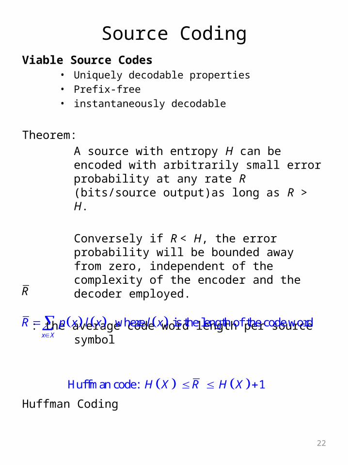
Source CodingViable Source Codes

• Uniquely decodable properties• Prefix-free• instantaneously decodable

Theorem: A source with entropy H can be encoded with arbitrarily small error probability at any rate R (bits/source output)as long as R > H.

Conversely if R < H, the error probability will be bounded away from zero, independent of the complexity of the encoder and the decoder employed.

: the average code word length per source symbol

Huffman Coding

where is the length of the code wordx X

R p x l x l x

R

Huffman code: 1H X R H X

23

QuantizationQuantization Function:

Squared-error distortion for a single measurement:

Distortion D for the source since X is a random variable

In general, a distortion measure is a distance between X and its reproduction .

Hamming distortion:

ˆ for all i iQ x x x

2 2ˆ,d x x x Q x x %

2ˆ,D E d X X E X Q X

ˆ1,

ˆ,0, Otherwiseh

x xd x x

X̂

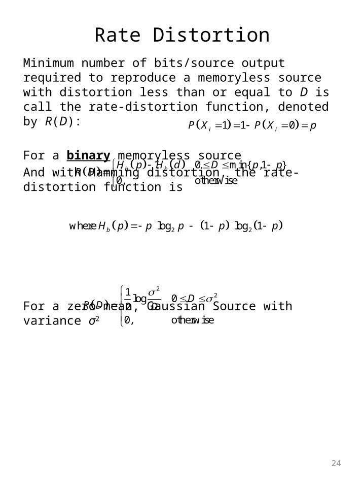
24

Rate DistortionMinimum number of bits/source output required to reproduce a memoryless source with distortion less than or equal to D is call the rate-distortion function, denoted by R(D):

For a binary memoryless sourceAnd with Hamming distortion, the rate-distortion function is

For a zero-mean, Gaussian Source with variance σ2

1 1 0i iP X P X p

0 min{ ,1 }

0, otherwiseb bH p H d D p p

R D

2

21log 0

20, otherwise

DR D D

2 2where log 1 log 1bH p p p p p

25

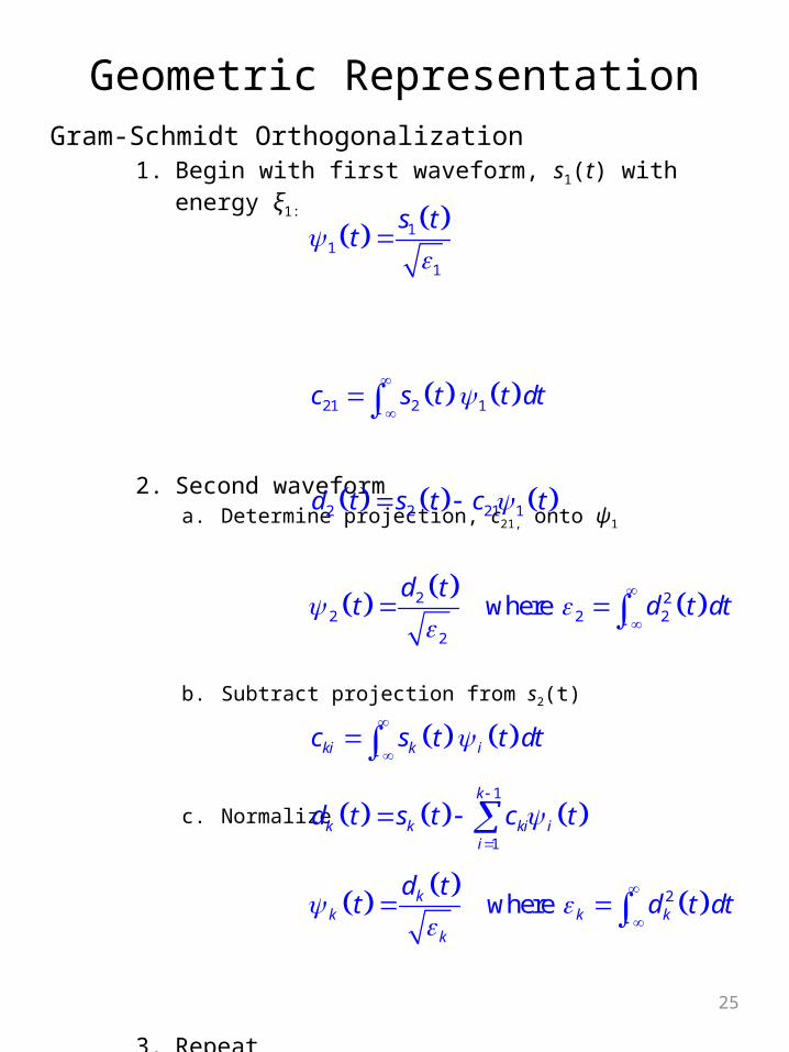
Geometric RepresentationGram-Schmidt Orthogonalization

1. Begin with first waveform, s1(t) with energy ξ1:

2. Second waveforma. Determine projection, c21, onto ψ1

b. Subtract projection from s2(t)

c. Normalize

3. Repeat

11

1

s tt

21 2 1c s t t dt

2 2 21 1d t s t c t

2 22 2 2

2

where d t

t d t dt

ki k ic s t t dt

1

1

k

k k ki ii

d t s t c t

2where kk k k

k

d tt d t dt

26

Pulse Amplitude ModulationBandpass Signals

What type of Amplitude Modulation signal does this appear to be?

X Baseband Signal

ms t

cos 2 cf t

Bandpass Signal

cos 2m cs t f t

cos 2 1, 2, ... ,

2

m m T c

mm T c T c

u t A g t f t m M

AU f G f f G f f

2

2 2 2

2 22 2

cos 2

cos 42 2

m m

m T c

m mT T c

u t dt

A t g t f t dt

A Ag t dt g t f t dt

0

27

PAM SignalsGeometric Representation

M-ary PAM waveforms are one-dimensional

where

For Bandpass:

1,2,...,m ms t s t m M

10

1,2,...,

T

g

m g m

t g t t T

s A m M

d d d d d

0

d = Euclidean distance between two points

g g

1

2

1

2

1

2

1

2 1

1

3

M

avg mm

Mg

Mm

Mg

m

g

M

AM

m MM

M

2cos 2 0

1,2,...,2

T cg

gm m

t g t f t t T

s A m M

28

Optimum ReceiversStart with the transmission of any one of the M-ary signal waveforms:

1. Demodulatorsa. Correlation-Typeb. Matched-Filter-Type

2. Optimum Detector3. Special Cases (Demodulation and Detection)

a. Carrier-Amplitude Modulated Signalsb. Carrier-Phase Modulation Signalsc. Quadrature Amplitude Modulated Signalsd. Frequency-Modulated Signals

Demodulator Detector mr t s t n t

Sampler

OutputDecision

2 symbols having -bits , 1, 2,...,

Transmitted within timeslot 0

Corrupted with AWGN:

km

m

M k s t m M

t T

r t s t n t

g

g

g

1 2, ,..., Nr t r r r r

ms Tr

29

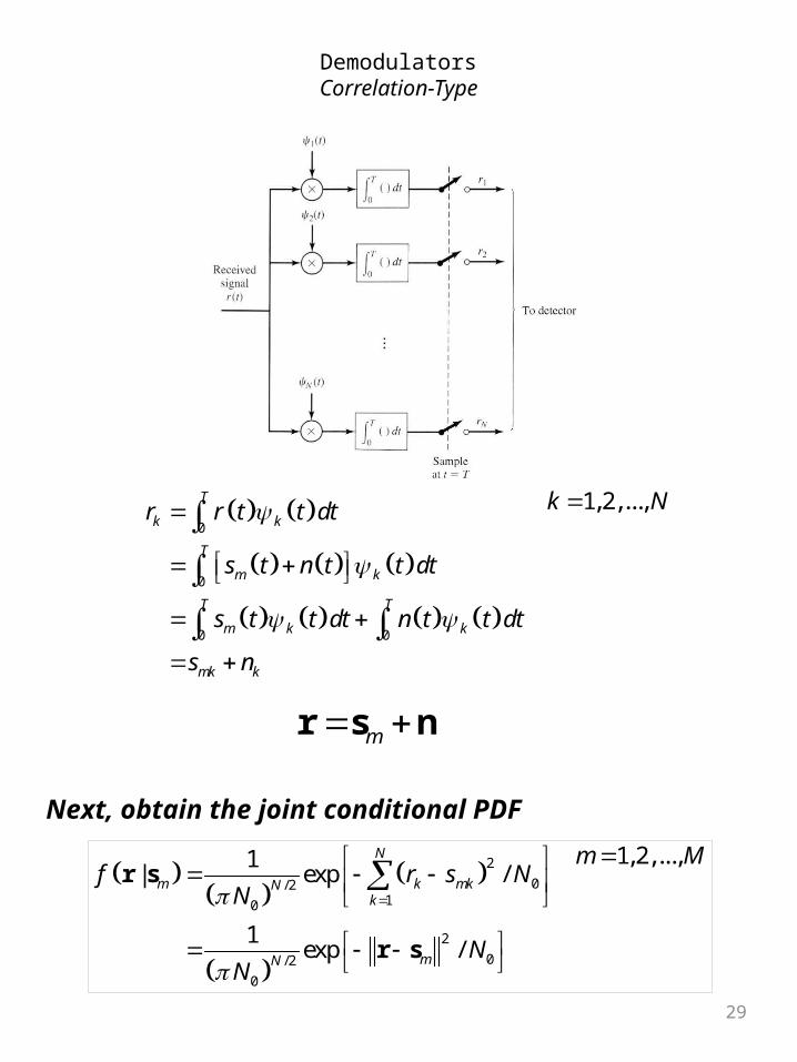
DemodulatorsCorrelation-Type

0

0

0 0

1,2,...,T

k k

T

m k

T T

m k k

mk k

k Nr r t t dt

s t n t t dt

s t t dt n t t dt

s n

m r s n

2

0/210

2

0/2

0

1,2,...,1| exp /

1exp /

N

m k mkNk

mN

m Mf r s N

N

NN

r s

r s

Next, obtain the joint conditional PDF

30

DemodulatorsMatched-Filter Type

Instead of using a bank of correlators to generate {rk}, use a bank of N linear filters.

The Matched Filter

Demodulator

Key Property: if a signal s(t) is corruptedby AGWN, the filter with impulse response matched to s(t) maximizes the output SNR

31

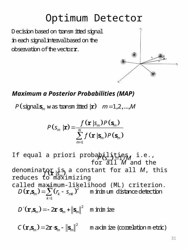
Optimum Detector

Maximum a Posterior Probabilities (MAP)

If equal a priori probabilities, i.e., for all M and the denominator is a constant for all M, this reduces to maximizing called maximum-likelihood (ML) criterion.

Decision based on transmitted signal

in each signal interval based on the

observation of the vector .r

signal was transmitted | 1,2,...,mP m Ms r

1

||

|

m mm N

m mm

f s PP s

f P

r s

rr s s

1/mP s M

| mf sr

2

1

2

2

, minimum distance detection

, 2 minimize

, 2 maximize (correlation metric)

N

m k mkk

m m m

m m m

D r s

D

C

r s

r s r s s

r s r s s

32

Probability of ErrorBinary PAM Baseband Signals

Consider binary PAM baseband signalswhere is an arbitrary pulse which is nonzero in the interval and zero elsewhere. This can be pictured geometrically as

Assumption: signals are equally likely and that s1 was transmitted. Then the received signal is

Decision Rule:

The two conditional PDFs for r are

1 2 Ts t s t g t Tg t

0 t T

02s 1s

b b

1 br s n n

1s

2sr 0

2

0

2

0

/

1

0

/

2

0

1| e

1| e

b

b

r N

r N

f r sN

f r sN

33

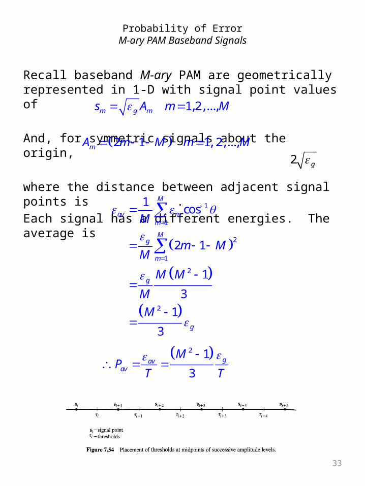
Probability of ErrorM-ary PAM Baseband Signals

Recall baseband M-ary PAM are geometrically represented in 1-D with signal point values of

And, for symmetric signals about the origin,

where the distance between adjacent signal points is .Each signal has a different energies. The average is

1,2,...,m g ms A m M

2 1 1, 2,...,mA m M m M 2 g

1

1

2

1

2

2

1cos

2 1

1

3

1

3

M

av mm

Mg

m

g

g

M

m MM

M M

M

M

2 1

3gav

av

MP

T T