Course FM/2 Practice Exam 2 – Solutions

Solutions Course FM/2 Practice Exam 2

© ActuarialBrew.com 2014 Page 1

Course FM/2 Practice Exam 2 – Solutions

Solution 1

E Nominal discount rate

The equation of value is:

4 10 4 5(4) (4)

25,000 1 30,000 1 146,842.604 4d d

We let 20(4)

14d

x

, and we can determine x using the quadratic equation:

2

2

25,000 30,000 146,842.60 0

30,000 30,000 4(25,000)( 146,842.60)2(25,000)

1.89674

x x

x

x

We discard the negative solution to the above equation since it doesn’t make sense for interest rates. We can now solve for the nominal discount rate convertible quarterly:

20(4)

20(4)

(4)

(4)

(4)

1 1.896744

1 0.527224

1 0.968504

0.3154

0.126

d

d

d

d

d

Solution 2

A Forward price and premium

We can determine the forward price from the forward premium:

0, 1.077884 75 80.8413TF



Once we have determined the forward price, we can determine the continuously paid dividend rate since it is the only remaining unknown value:

( )0, 0

(0.15 )0.75

0.15 0.75 0.75

0.75

80.8413 75

80.8413 75

0.96319ln(0.96319)

0.750.050

r TTF S e

e

e e

e

Solution 3

B Annuity-due accumulated value factor

Jackie makes monthly deposits of $X into her retirement account from her 22nd birthday until one month before she turns 55. She makes these deposits from age 22 through age 54, so the total number of monthly deposits is (54 22 1) 12 396 . The monthly effective interest rate is:

(12) 0.060.005

12 12i

The accumulated value of these deposits at age 55 is:

396 0.5%Xs

Starting at age 55, Jackie receives monthly retirement payments of $5,000 until one month before she turns 89. She receives these payments from age 55 through age 88, so the total number of monthly payments is (88 55 1) 12 408 . The present value of these payments at age 55 is:

408

408 0.5%1 1.005

5,000 5,000 873,655.20560.005 /1.005

a

Since Jackie would like to deplete her retirement savings account, we can equate the accumulated value of her deposits at age 55 with the present value of her payments at age 55 and solve for the unknown deposit X:

396 0.5%396

873,655.2056

1.005 1873,655.2056

0.005 /1.005700.2536

Xs

X

X



Solution 4

D Stock price: dividend discount model

This problem is complicated by the fact that the dividend payments within each year are level, but dividend increases occur annually. One fairly straightforward approach to this complication is to reframe the problem so as to mimic annual payments with annual increases, and then we can use the annual compound increasing annuity factor. We perform an intermediate series of present value calculations to answer this type of question more quickly.

The quarterly effective interest rate is (4)

1 / 4(1.0825) 1 0.020024i

.

During the first year, a payment of $5 is made at the end of each quarter. The present value of the first year’s quarterly dividend payments at time 0 is 4 2.002%5a .

During the second year, a payment of $5(1.03) is made at the end of each quarter. The present value of the second year’s dividend payments at time 1 is 4 2.002%5(1.03)a .

During the third year, a payment of 25(1.03) is made at the end of each quarter. The

present value of the third year’s dividend payments at time 2 is 24 2.002%5(1.03) a .

Once we recognize this pattern, we see that we have created a series of annual payments with annual increases that has the same present value as the original, more complicated series of quarterly payments. We have conveniently converted our complicated series of quarterly payments that occur at the end of each quarter to an equivalent series of payments that occur at the beginning of each year.

We can factor out 4 2.002%5a from this equivalent series of annual payments and we are

left with a payment of 1 at time 0, 1.03 at time 1, 21.03 at time 2, and so on. This matches the pattern of a compound increasing perpetuity-due. The present value of a compound increasing perpetuity-due is:

1 (1 ) 1

lim lim where /(1 ) 1

n

j n jn n

j j i ea a j

j j j e

In this case, (0.0825 0.03) /1.03 0.05097j .

The present value of the dividends is then:

4

4 2.002% 5.097%1 1.002002 1.05097

5 5 392.54350.002002 0.05097

a a

.



Solution 5

C Bond yield

Let’s work in semiannual effective periods and define the bond variables first:

40

1,00020 2 40

/ 2

(1 ) 156.25585.23

Fni r

K C iP

The price of a bond can be written as:

n iP rFa K

With a little substitution are re-arranging, we see that / 2r i and we can solve for the semiannual effective interest rate i:

40

40

40

40

1 (1 )585.23 1,000 156.25

2

428.98 500 1 (1 )

0.85796 1 (1 )

0.14204 (1 )1 1.050001

0.050001

i ii

i

i

iii

Since this is the semiannual effective interest rate, we need to determine the annual effective yield rate:

21.005001 1 0.102502

Solution 6

D Nominal interest rate

Let’s work in semiannual payments and define j as the semiannual effective interest rate. Since the accumulated value at time 20 years is five times the accumulated value at time 10 years, the equation of value is:

20 40

20 40

20 40

40 20

5

(1 ) 1 (1 ) 15

5[(1 ) 1] (1 ) 1

(1 ) 5(1 ) 4 0

j jYs Ys

j jj j

j j

j j



Let 20(1 )x j , and we can solve the above equation for x:

2

2

5 4 0

( 5) ( 5) 4(1)(4)2(1)

4 or 1

x x

x

x

We have:

20 20(1 ) 4 (1 ) 1

1 1.07177 1 10.07177 0

i or i

i ii i

Since this is the semiannual effective interest rate, we need to convert it to the annual nominal rate convertible semiannually:

(2) 2 0.07177 0.143547i

Solution 7

A Time to accumulate assuming annual effective interest rate

The accumulated value of the payments of $5,000 during the first 2n years at time 2n years is:

25,000 ns

This accumulated value needs to be accumulated for another 4n years to bring it to time 6n years.

The accumulated value of the payments of $10,000 during the second 2n years at time 4n years is:

210,000 ns

This accumulated value needs to be accumulated for another 2n years to bring it to time 6n years.

The accumulated value of the payments of 20,000 during the last 2n years at time 6n years is:

220,000 ns



The equation of value for Katrina’s accumulated value at time 6n years is:

4 22 2 2

4 22

2 4 2

2 4

500,000 5,000 (1 ) 10,000 (1 ) 20,000

500,000 5,000(1 ) 10,000(1 ) 20,000

500,000 (1 ) 1 5,000(1 ) 10,000(1 ) 20,000

500,000 1.28 1 5,000(1.28) 10,000(1.2

n nn n n

n nn

n n n

s i s i s

s i i

i i i i

i

28) 20,000

0.06359i

We then have:

(1.06359) 1.28ln(1.28)

ln(1.06359)4.004

n

n

n

Solution 8

A Varying force of interest and varying payments

The present value at time 0 of the $1,000 payment at time 5 years is:

2

50

5( / 200)

( /100) 0 (25 / 200 0)1,000 1,000 1,000 882.4969t

t dte e e

The present value at time 0 of the $2,000 payment at time 10 years is:

2

100

10( / 200)

( /100) 0 (100 / 200 0)2,000 2,000 2,000 1,213.0613t

t dte e e

The total present value is 882.4969 1,213.0613 2,095.5582 . To determine the annual effective interest rate in effect over this period, we set up another equation of value for

this accumulated value, let 5(1 )x i , solve for x and then i:

5 10

2

2

5

1,000(1 ) 2,000(1 ) 2,095.5582

2 2.0955582 0

1 1 4(2)( 2.0955582)2(2)

0.80370

(1 ) 0.803701 1.04468

0.04468

i i

x x

x

x

ii

i

We discarded the negative solution for x since it didn’t make sense for an interest rate.



Solution 9

E Short sale

Using the equation for the yield on a short sale, we solve for the unknown variable, M:

(margin )(margin req %)( ) div yield

(margin req %)( )(100 95) 5 3

0.093100

0.093 0.070.7527

S B i SSS

S

MMM

Solution 10

C Callable bond yield


1,00015 2 300.04 / 2 0.02

coupon 0.02 1,000 2020 /1,000 0.02

F Cnr

g

Since the price of the bond is greater than the redemption amount, the bond is a premium bond, and g > i. The minimum yield is determined from a call at the earliest possible call date for a premium bond. (If the call price changes, then we would need to check the price at the earliest date of each call price change.) The earliest call date in this case is to assume that the bond is called at time 10 years, or at time 20 semiannual periods. However, since the call price effectively changes at maturity when the bond is redeemed for $1,000 instead of the call price of $1,050, we need to also check the yield at time 15 years, or at time 30 semiannual periods, and the minimum yield will be whichever is lower.

Let’s check the first case assuming the bond is called at time 10 years. Using the BA-35 calculator, we press [2nd][CMR], 1,050 [FV], 20 [PMT], 1,100 [PV], 20 [N], and [CPT][%i], and the result is 1.62400. Using the BA II Plus, we press [2nd][CLR TVM], –1,050 [FV],

20 [PMT], 1,100 [PV], 20 [N], and [CPT][I/Y], and the result is the same.

Let’s check the second case assuming the bond matures at time 15 years. With bonds, it is assumed that a bond matures at the par amount unless otherwise stated. Using the BA-35 calculator, we press [2nd][CMR], 1,000 [FV], 20 [PMT], 1,100 [PV], 30 [N], and [CPT][%i], and the result is 1.57893. Using the BA II Plus, we press [2nd][CLR TVM],

1,000 [FV], –20 [PMT], 1,100 [PV], 30 [N], and [CPT][I/Y], and the result is the same.

The lower yield occurs with the second case, so this is the minimum yield. This interest rate is the semiannual effective interest rate. The corresponding annual nominal rate convertible semiannually is 0.015789 2 0.031579 .



We can verify that this is the minimum return by calculating the yields if the bond had been called at other dates. If a yield at another possible call date is lower, then it would be the minimum yield. The table below illustrates the semiannual effective yields at other chosen call dates:

N Yield

21 0.01635

22 0.01645

… …

29 0.01696

Since no other semiannual effective yield is lower than 0.01579, the minimum yield expressed as an annual nominal rate convertible semiannually is 3.1579%.

Solution 11

D Collar

A purchased collar resembles a short forward contract, not a written collar.

Solution 12

B Continuous payment accumulated value

Since the payments occur from time 2 to time 8 years, the accumulated value at time 8 years is:

888 8 ln( 5)

[1 /( 5)]2,8

2 28 8

[ln13 ln( 5)]

2 28 8

2 2

100( 5) 100( 5)

13100( 5) 100( 5)

5

8100 13 1,300 1,300 1,300(8 2)

2

7,800

ts

s ds t

t

AV t e dt t e dt

t e dt t dtt

dt dt t



Solution 13

B Bond yield assuming reinvestment of coupons


60

60 2.75%

1,0001,07530 2 600.065/ 2 0.0325

coupon 0.0325 1,000 32.50coupon reinvesment rate 0.055/ 2 0.0275

(1.0275) 1148.80914

0.0275

F CPnr

s

The accumulated value of the coupons at time 30 years is:

60 2.75%32.50 32.50(148.80914) 4,836.29706s

The bond is redeemed for $1,000 at time 30 years, so the value of the bond at time 30 years is:

4,836.29706 1,000 5,836.29706

To determine the annual effective yield over the 30-year period, we set up the equation of value and solve for i:

30

30

1,075(1 ) 5,836.29706

(1 ) 5.429110.058013

i

ii

The annual effective yield can also be determined using a financial calculator. Using the BA 35, we press [2nd][CMR], 5,836.29706 [FV], 30 [N], 0 [PMT], 1,0754 [PV], [CPT][%i], and the result is 5.80129. Using the BA II Plus, we press [2nd][CLR TVM], 5,836.29706 [FV], 30 [N], –1,075 [PV], 0 [PMT], [CPT][I/Y], and we get the same result.

We still need to convert this annual effective yield to a annual nominal yield rate convertible semiannually. We have:

1 / 2(2) 2[(1.058013) 1] 0.057195i

Solution 14

C Dollar and time-weighted interest rates

Let’s denote i as the annual effective interest rate. Using the information for account A, the equation of value for the dollar-weighted interest rate is:

12 /12 (12 3) /12 (12 9) /12970 1,000(1 ) 150(1 ) 300(1 )i i i



Since this activity occurs during a 12-month period, we can use the simple interest approximation to solve for the annual effective interest rate i:

12 9 3970 1,000(1 ) 150(1 ) 300(1 )

12 12 12970 1,000 1,000 150 112.5 300 751,037.5 120

0.11566

i i i

i i ii

i

Since the time-weighted return of account B equals the dollar-weighted return of account A, we set up the equation of value for the time-weighted interest rate and solve for the unknown variable X:

1 1,080 1,595(1 ) 1.11566

1,000 1,080 31,722.60 1,204.91566 3.34699

517.68434 3.34699154.672

iX

XX

X

Solution 15

D Dedication

Since all three bonds have an annual effective yield of 6%, all of the liability cash flows are discounted at 6%, and we can quickly determine the answer:

2 3

1,000,000 1,500,000 2,000,0003,957,629.45

1.06 1.06 1.06

An alternative approach involves a little more work, but it is still a valid approach. The liability cash flows of 1.0 million at time 1, 1.5 million at time 2, and 2.0 million at time 3 must be matched exactly by the asset cash flows. Assuming that the bonds each have a par value of $1,000, the asset cash flows are illustrated in the following table:

Bond Time 1 Time 2 Time 3

1-year 1,050 N/A N/A

2-year 60 1,060 N/A

3-year 70 70 1,070

To match the liability cash flows with asset cash flows, we need to work backward from time 3. At time 3, we need 2.0 million in asset cash flows, so the number of 3-year bonds required is:

2,000,000

1,869.15891,070



At time 2, we need 1.5 million in asset cash flows, but we already have 1,869.1589 of the 3-year bonds. The 3-year bonds at time 2 pay 1,869.1589 70 130,841.1215 . The net liability cash flow at time 2 that must be matched by the 2-year bond is then 1,500,000 130,841.1215 1,369,158.879 .

So, the number of 2-year bonds required is:

1,369,158.879

1,291.659321,060

At time 1, the 3-year bonds pay 1,869.1589 70 130,841.1215 and the 2-year bonds pay 1,291.65932 60 77,499.5592 . The net liability cash flow that must be matched by the 1-year bond is then 1,000,000 130,841.1215 77,499.5592 791,659.3193 . So, the number of 1-year bonds required is:

791,659.3193

753.96131,050

The prices of each of the bonds are:

1

2 2

3 2 3

1,050990.5660

1.0660 1,060

1,000.001.06 1.0670 70 1,070

1,026.73011.06 1.06 1.06

yr

yr

yr

P

P

P

The cost to the insurance company to exactly match its liability cash flows is:

753.9613 990.5660 1,291.6593 1,000 1,869.1589 1,026.73013,957,629.45

X



Solution 16

C Portfolio yield method

The portfolio rates are in the rightmost column of the table. The portfolio rates come after three years of investment year rates. To get the portfolio yield rate in effect for 2004, we read across the 2001 row, so the portfolio rate in effect for 2004 is 7.6%. Similarly, the portfolio rates in effect for 2005, 2006 and 2007 are 7.75%, x% and 8.3%, respectively.

A deposit of $50,000 was made on 1/1/04 and we know that the accumulated value on 1/1/08 is $67,803.45. It is a straightforward matter to set up the equation of value and solve for x:

67,803.45 (50,000)(1.0760)(1.0775)(1 )(1.0830)67,803.45

162,780.9685

1.080 10.080

x

x

xx

Solution 17

D Macaulay duration of bond

We need to pay close attention to how the yield is expressed in this type of question before we decide which formula to use. In this case, the yield was given as a continuously compounded yield, i.e., as a force of interest.

Macaulay duration is the negative of the derivative of the price function with respect to the continuously compounded yield. The Macaulay duration is:

'( ) 1( )

P dPMacD

P d P

Since we have been given the derivative of the price of the bond with respect to the yield expressed as a continuously compounded force of interest, we have already been given the numerator of the Macaulay duration formula. We can therefore determine the answer with a straightforward application of the Macaulay duration formula:

1 1

( 800) 7.4998106.67

dPMacD

d P



If the question had provided the price of the bond with respect to the yield expressed as a nominal yield compounded m times per year instead, then we would have been given the numerator of the Modified duration formula. Modified duration is the negative of the derivative of the price function with respect to the nominal yield y compounded m times per year:

'( )( )

P yModD

P y

Usually for bonds, the yield y is expressed as the nominal yield compounded twice per year since bond coupons occur twice per year. If the yield had been expressed this way, then we would have calculated Modified duration first. We could then convert Modified duration to Macaulay duration:

1

MacDModD

ym

Solution 18

E Decreasing annuity-due accumulated value

The payments start at $375 at time 0 and decrease by $25 each year. There are 15 payments, so the last payment of $25 occurs at time 14 years. This fits the pattern of a decreasing annuity-due with a factor of $25. The accumulated value at time 15 years is:

15 6%25( )Ds

Since we need to determine the accumulated value at time 20 years, we need to accumulate the time 15 year accumulated value for 5 more years. The required values are:

15

15 6%

15

15 6%

1.06 123.27597

0.06

15(1.06) 23.27597( ) 223.87912

0.06 /1.06

s

Ds

The accumulated value at time 20 years is:

515 %25( ) (1.06) 25(223.87912)(1.33823) 7,490.0191Ds

Solution 19

A Increasing annuity-due accumulated value

The level payments are $50 at the beginning of each year, starting at time 0 and ending with the 15th payment at time 14 years. After this point, each payment is $5 more than the preceding payment. At time 15, the payment is $55, and since the payments increase by $5 each year for 10 years, the last payment is $100 at time 24 years.



Let’s split these payments into two parts. The first part is the level annuity-due from time 0 to time 24 years and the second part is the increasing annuity-due from time 15 to time 24 years, starting at $5 at time 15 years and increasing to $50 at time 24 years.

The accumulated value of the first part at time 25 years is:

25

25 7%1.07 1

50 50 3,383.823520.07 /1.07

s

The second part fits the pattern of a 10-year increasing annuity-due with the first payment occurring at time 15 and the last payment occurring at time 24 years. The accumulated value of the second part at time 25 years is:

10 7%5( )Is

Determining the required values, we have:

10

10 7%

10 7%10 7%

1.07 114.78360

0.07 /1.0710

( ) 73.120730.07 /1.07

s

sIs

So the accumulated value of the second part at time 25 years is:

5(73.12073) 365.60366

The accumulated value of both parts at time 25 years is:

3,383.82352 365.60366 3,749.4272

Solution 20

E Refinance an annual payment loan

There are 30 annual payments and the annual effective interest rate is 6.5%. Let’s determine the appropriate annuity present value factor before we get started:

30

30 6.5%1 1.065

13.058680.065

a

We determine the initial loan amount:

30 6.5%

5,000 13.05868

65,293.37953

LP

a

L

L



The balance of the loan at time 5 years using the prospective method is the present value of the remaining loan payments:

25

5 25 6.5%1 1.065

5,000 5,000 60,989.383630.065

B a

Alternatively, the balance of the loan at time 5 years using the retrospective method is the accumulated value of the initial loan amount less the accumulated value of the loan payments:

55 5 6.5%

55

65,293.37953(1.065) 5,000

1.065 165,293.37953(1.065) 5,000

0.06560,989.38363

B s

At this time, the borrower borrows an additional $10,000, which is added to the loan balance. The new loan balance that must be paid off over the next 20 years is 60,989.38363 10,000 70,989.38363 .

The revised premium payment is then:

20

20 6.5%

70,989.38363 70,989.383636,442.74

1 1.0650.065

Pa

Solution 21

C Deferred interest rate swap

The zero-coupon bond prices are:

1

2

3

4

(0,1) 1.0425 0.959233

(0,2) 1.0475 0.911364

(0,3) 1.0525 0.857697

(0,4) 1.0575 0.799611

P

P

P

P

The 1-year implied forward rates are:

0 02

0

3

0 2

4

0 3

(0,1) 0.0425 (not used in solution)

1.0475(1,2) 1 0.052524

1.0425

1.0525(2,3) 1 0.062572

1.0475

1.0575(3,4) 1 0.072643

1.0525

r s

r

r

r



The 1-year deferred fixed swap rate is:

0 0 0(0,2) (1,2) (0,3) (2,3) (0,4) (3,4)(0,2) (0,3) (0,4)

0.911364(0.052524) 0.857697(0.062572) 0.799611(0.072643)0.911364 0.857697 0.799611

0.1596220.0621

2.568671

P r P r P rR

P P P

A quicker way to determine the answer is:

(0,1) (0,4) 0.959233 0.7996110.0621

(0,2) (0,3) (0,4) 2.568671P P

RP P P

Solution 22

B Varying monthly payments present value expression

The $500 payments occur monthly from time month 3 to month 302. The $600 payments begin at the next month (month 303) and occur monthly from time month 303 to month 602. The $750 payments begin at the next month (month 603) and occur monthly from month 603 to 902. The $800 payments begin at the next month (month 903) and occur monthly from month 903 to 1,202.

The annual effective interest rate is i and the monthly effective interest rate is j. The payments occur monthly, so we’ll work in monthly periods.

Since the first payment does not occur until time 3 months, the annuity-immediate present value factor for the first 60 payments is valued one month before the first payment, or at time 2 months.

The present value factor of the $500 payments needs to be discounted back 2 months to time 0. The present value at time 0 of the $500 payments from the first 5-year period is:

260(1 ) 500 jj a

The present value factor of the $600 payments needs to be discounted back 302 months (5 years and 2 months) to time 0. The present value at time 0 of the $600 payments from the next 5-year period is:

2 560(1 ) (1 ) 600 jj i a


2 1060(1 ) (1 ) 750 jj i a




2 1560(1 ) (1 ) 800 jj i a

Putting them all together, we have:

2 2 560 60

2 10 2 1560 60

(1 ) 500 (1 ) (1 ) 600

(1 ) (1 ) 750 (1 ) (1 ) 800

j j

j j

j a j i a

j i a j i a

Simplifying, we have:

2 5 10 1560

2 5 10 1560

100,000 (1 ) 500 [1 1.2(1 ) 1.5(1 ) 1.6(1 ) ]

200 (1 ) [1 1.2(1 ) 1.5(1 ) 1.6(1 ) ]

j

j

j a i i i

j a i i i

Solution 23

A Sinking fund balance

Using the amortization method, we determine the annual payment P:

15

15 7%

25,000 25,0002,744.86562

1 1.070.07

Pa

The sinking fund payment in this case is equal to $P less the interest on the loan:

2,744.86562 25,000(0.07) 994.86562SFP

At the end of 15 years, the accumulated value of the sinking fund payments is used to pay off the loan amount of $25,000. Using the sinking fund annual effective interest rate of 10%, the accumulated value of the sinking fund payments at time 15 years is:

15

1510%1.10 1

994.86562 994.86562 31,609.349620.10

s

The sinking fund balance immediately after the repayment of the loan is:

31,609.34962 25,000 6,609.34962



Solution 24

B Reinvestment of interest at different rate than initially earned

At the end of the first year, the time 0 $500 investment pays interest of 500 0.06 30 . This is then reinvested at an annual effective interest rate of 4% for 24 years until time 25. At time 1, the account contains the $500 deposit from time 0 plus a new $500 deposit at time 1. So and the end of the second year, the two $500 deposits pay interest of 2 500 0.06 2 30 . This is then reinvested at an annual effective interest rate of 4% for 23 years until time 25. At time 2, the account contains the two prior $500 deposits plus a new $500 deposit at time 2. So at the end of the third year, the three $500 deposits pay interest of 3 500 0.06 3 30 . This is then reinvested at an annual effective interest rate of 4% for 22 years until time 25.

Recognizing a pattern, we can now write the equation of value for the accumulated value at time 25, which includes the 25 deposits of $500 and the interest which is reinvested at a different rate than it was initially earned:

24 23 22 025 500 30(1.04) 2 30(1.04) 3 30(1.04) 25 30(1.04)

Rearranging the terms, we recognize the pattern for the accumulated value of an increasing annuity-immediate:

24 23 22 012,500 30[1 (1.04) 2 (1.04) 3 (1.04) 25 (1.04) ]

The part in the brackets is 25 4%( )Is . Calculating this required value, we have:

25

25 4%25 4%

1.04 125

0.04 /1.0425( ) 457.79362

0.04 0.04

sIs

The accumulated value at time 25 years is then:

12,500 30[457.79362] 26,233.80846

To determine the annual effective yield on the entire investment over the 25-year period, we set up the equation of value using an annuity-due accumulated value factor since the $500 payments are made at the beginning of each year. We need to solve for i:

2526,233.80846 500 is

With a financial calculator, the annual effective yield over the 25-year period can be quickly determined. Using the BA 35, we press [2nd][CMR], [2nd][BGN], 26,333.80846 [FV], 25 [N], 500 [PMT], [CPT][%i], and the result is 5.3105. Using the BA II Plus, we press [2nd][CLR TVM], [2nd][BGN] [2nd][SET] [2nd]{QUIT], –26,333.80846 [FV], 25 [N], 500 [PMT], [CPT][I/Y], and we get the same result.



Solution 25

A Classic immunization

To satisfy the first condition of classic immunization, the present value of the assets must equal the present value of the liabilities. The present value of the liabilities is:

4

5,0004,113.51237

1.05LPV

To satisfy the second condition, the Macaulay duration of the asset portfolio must equal the Macaulay duration of the liabilities. The Macaulay duration of the liabilities is:

41 4 5,000 1.054.0

4,113.512371

mtyt m

mtyt m

tCFMacD

CF

For a security with one cash flow, the Macaulay duration is just the time of that single cash flow. We need to set up the asset portfolio so that it has a Macaulay duration of 4.0 years. We first determine the Macaulay duration of the 3-year and the 5-year bonds:

1 2 3

3 1 2 3

5

1 6 1.05 2 6 1.05 3 106 1.05 291.2989962.83576

102.7232486 1.05 6 1.05 106 1.055.0

yr

yr

MacD

MacD

Since the 5-year bond just has one cash flow, its Macaulay duration is the time of that cash flow. Now we need to determine how much to invest in the 3-year bonds. We let x denote the percent of the asset portfolio to invest in the 3-year bonds. We equate the Macaulay duration of the asset portfolio to the Macaulay duration of the liability portfolio, and we solve for x:

3 5(1 )

2.83577 5(1 ) 4.02.16423 1.0

0.46206

yr yr LxMacD x MacD MacD

x xx

x

So we invest 46.206% of the asset portfolio in the 3-year bonds. The total asset portfolio has a value of $4,113.51237, so the amount invested in the 3-year bond is:

4,113.51237 0.46206 1,900.6774

Since we have determined the answer, during the exam we would just stop here and move on to the next question. But just to make sure that we have immunized the portfolio, we can check the third condition of immunization, which requires that the Macaulay convexity of the asset portfolio be greater than the Macaulay convexity of the liability portfolio. The Macaulay convexity of the liabilities is:

2 4

24 5,000 1.054.0 16

4,113.51237MacC



For a security with one cash flow, the Macaulay convexity is the square of the time of that cash flow. The Macaulay convexities of the 3-year and 5-year bonds are:

2 1 2 2 2 3

3

25

1 6 1.05 2 6 1.05 3 106 1.058.28743

102.723248

5 25

yr

yr

MacC

MacC

We already know the percentages of the asset portfolio invested in the 3-year and 5-year bonds. We can determine the Macaulay convexity of the asset portfolio, and we see that it does in fact exceed that of the liabilities, so condition three is satisfied:

0.462057 8.28743 (1 0.462057)(25) 17.2778AMacC

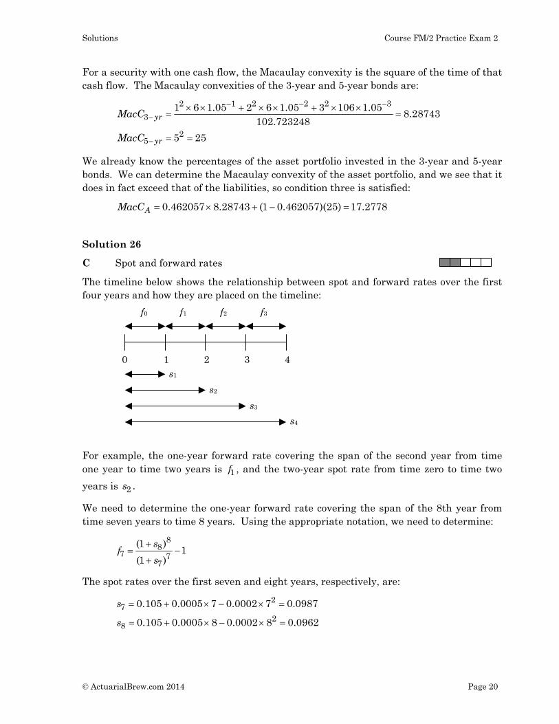
Solution 26

C Spot and forward rates

The timeline below shows the relationship between spot and forward rates over the first four years and how they are placed on the timeline:

f0

0 1 2 3 4

f1 f2 f3

s1

s2

s3

s4

For example, the one-year forward rate covering the span of the second year from time one year to time two years is 1f , and the two-year spot rate from time zero to time two

years is 2s .

We need to determine the one-year forward rate covering the span of the 8th year from time seven years to time 8 years. Using the appropriate notation, we need to determine:

8

87 7

7

(1 )1

(1 )

sf

s

The spot rates over the first seven and eight years, respectively, are:

2

72

8

0.105 0.0005 7 0.0002 7 0.0987

0.105 0.0005 8 0.0002 8 0.0962

s

s



We have:

8

7 71.0962

1 0.078861.0987

f

Solution 27

D Annuity relationships

Statement I is true since:

1

2

2 11

1

1

so

1

nn

nn

nn

n n

a v v

a v v v

a v v v

a a

Statement II is false since:

1 (1 ) (1 ) 1

(1 ) 1 (1 ) 1 (1 ) 1 1

n n n

n n n n nn n

i i i i i i i v ii i

s ai i i v v

Statement III is false since:

1 1

1 (1 )n m

n m m nn m

v vi a a i v v v v

i i

Solution 28

E Prepaid forward price

The prepaid forward price is the current stock price less the present value of the future dividends over the ten-year period. Since the dividends are paid quarterly, let’s work in quarters to determine the present value of the dividends. There will be 40 dividends over the ten-year period, and the quarterly effective interest rate is:

(4)

0.25(1.10) 1 0.0241144i

The prepaid forward price is:

0, 40 2.4114%

40

65 0.75

1 1.02411465 0.75

0.024114

45.89

PTF a



Solution 29

E Net present value

Typically, an investment requires a cash outflow at time 0, and the cash inflows usually commence after time 0. In this case, the cash outflow occurs at time 1, so it must be discounted for 1 year to determine its present value at time 0. The cash inflows start at time 5 years, and there are 10 annual payments from time 5 years to time 14 years inclusive. If we use an annuity-immediate present value factor to value these cash flows, its value would be at time 4 years, i.e., one year before the first cash flow, so it must be discounted for 4 years to determine its present value at time 0.

The net present value of this investment is:

1 410 9%

10

50,000(1.09) 11,000 (1.09)

1 1.0945,871.5596 11,000 (0.70843)

0.09

4,139.176

NPV a

Solution 30

C Written strangle

A written strangle involves selling a lower-strike put and selling a higher-strike call, which is depicted by answer choice C.

Answer choice A is a written straddle, which consists of a short put and a short call with the same strike price and time to maturity.

Answer choice B is a purchased straddle, i.e., a long put and a long call with the same strike price and time to maturity.

Answer choice D is a purchased strangle, which involves buying a lower-strike put and selling a higher-strike call.

Answer choice E is a butterfly spread, which is otherwise known as an insured written straddle.

Solution 31

D Loan balance

Notice that the loan payment is not enough to cover the interest due on the loan. The annual loan payment is $15,000 but the annual interest due on the loan is:

250,000 0.07 17,500tI



The loan balance will increase over time as long as this situation occurs. If we were to use the prospective method, we would need to know the length of the loan, but that is not given and the loan will never be paid off as long as the loan payment is less than the interest due on the loan. So in this case, it is better to use the retrospective method. Using the retrospective method, we have:

1010 10 7%

10

250,000 1.07 15,000

1.07 1250,000 1.967151 15,000

0.07

284,541.12

B s

Using the BA II Plus, we enter 10 [N], 7 [I/Y], –250,000 [PV], 15,000 [PMT], and then [CPT][FV], and we get the same result, 284,541.12.

Solution 32

A Increasing perpetuity-due

The first payment of $1,000 occurs now. The second payment of $1,000 occurs in six months. The third payment of $1,100 occurs in one year. The fourth payment of $1,100 occurs in 18 months. This increasing payment pattern continues forever. There are two payments per year which occur every six months, but the increases of $100 occur annually. We can make a few adjustments before we apply our standard annuity formulas.

Let’s break these cash flows into two parts. The first part is a level series of payments of $900 that occurs every six months forever, with the first payment starting today. The second part is an increasing series of payments that occur every six months, in which the first and second payments are $100, the second and third payments are $200, the fourth and fifth payments are $300, and so on.

The first part is not that difficult to value since there are level payments of $900 that occur every six months. Working in six-month effective periods, we have:

(2)0.5

(2)

1.05 1 0.0246952

0.0246950.024100

2 1.024695

i

d

Continuing to work in six-month periods, the present value of the first part is:

1

900( ) 900 37,344.51140.024100

Ia



To value the second part, let’s look at the two payments that occur within the first year. We have a payment of $100 that occurs now and a payment of $100 that occurs at time six months. The present value at time 0 of these payments is:

2100a

The annuity factor in the above equation assumes semi-annual payments and uses semi-annual effective interest rates. Now let’s look at the two payments that occur within the second year. We have a payment of $200 that occurs at time one year and a payment of $200 that occurs at time 18 months. The present value at time 1 year of these payments is:

2200a

The annuity factor in the above equation once again assumes semi-annual payments and uses semi-annual effective interest rates. Now let’s look at the two payments that occur within the third year. We have a payment of $300 that occurs at time two years and a payment of $300 that occurs at time 30 months. The present value at time 2 years of these payments is:

2300a

Notice that we have now constructed a series of annual payments that increase by $100 each year. If we pull out a factor of 2100a from this series of payments, we are left with a

payment of $1 at time 0, $2 at time 1, $3 at time 2, and so on. This matches the pattern expected by one of our standard annuity formulas. Working in six-month periods, the present value of the factor is:

2

21 1.024695

100 100 197.5900070.024100

a

Shifting gears and working in annual periods for the remaining annual increasing cash flows without the factor, the present value is:

2

1( ) 441.00

(0.05 /1.05)Ia

Putting the two pieces together, we have:

37,344.5114 197.59007 441.00 124,481.70

Alternatively, we can determine this answer more quickly if we recognize that the payments made in the first semester of each of the years consists of an perpetuity-due of $1,000 per year and an increasing perpetuity annuity-immediate. The present value of this series of payments is:

2

1,000 100 1.051,000 100( ) 63,000

0.05 /1.05 0.05a Ia

The payments made in the second semester of each of the years are the same but they all occur six months later, so their present value is simply:

0.563,000(1.05) 61,481.7046



Add these two parts together, and we get the same answer as before:

63,000 61,481.7046 124,481.70

Solution 33

D Modified duration

Modified duration is calculated as:

'( )( )

P iModD

P i

We have:

4 6 4 6( ) 500 750(1 ) 1,000(1 ) 500 1 1.5 2P i i i v v

We determine the derivative of the price function with respect to yield:

5 7

5 7

7 5

'( ) 4(750)(1 ) 6(1,000)(1 )

3,000 6,000

3,000 2

P i i i

v v

v v

Modified duration is therefore:

7 5 5 7

4 6 4 6

3,000 2 26

500 1 1.5 2 1 1.5 2

v v v v

v v v v

Solution 34

C Derivative use

The investor expects two things. The investor expects the price of IBM stock to decrease along with the variability of the price of IBM stock. Selling calls is the best strategy in this case, so choice C is correct. See Table 3.9 in the text.

Buying puts is a good strategy if the investor expects the price to fall and the price variability to increase. Selling IBM shares is a good strategy if the investor expects the price to fall and has no view on price variability. Buying a straddle is a good strategy if the investor has no view on prices but expects the price volatility to increase. Selling a straddle is a good strategy if the investor has no price view but expects the price volatility to decrease.



Solution 35

E Put-call parity

The current time is t, and the time to expiration of the options is T, so the amount of time between now and expiration is T – t. Put-call parity says that the net cost of buying the stock using options must equal the net cost of buying the stock using a forward contract. The net cost of buying the call and selling the put plus the present value of the strike price is:

( )( , ) ( , ) r T tC K T t P K T t Ke

The net cost of buying the dividend-paying stock using a forward contract is:

( ),( ) T tt T tPV F S e

Rearranging these terms, we see that choice E is correct.

( ) ( )

( ) ( )

( , ) ( , )

( , ) ( , )

r T t T tt

r T t T tt

C K T t P K T t Ke S e

C K T t Ke S e P K T t

Documents

Course FM/2 Practice Exam 2 – Solutions