Course 2 38 May 2000

37. A customer is offered an investment where interest is calculated according to

the following force of interest:

0.02 0 3

0.045 3t

t t

t�

� ��� �

��

The customer invests 1000 at time t = 0 .

What nominal rate of interest, compounded quarterly, is earned over the first

four-year period?

(A) 3.4%

(B) 3.7%

(C) 4.0%

(D) 4.2%

(E) 4.5%

Français Webcasts Email Alerts Contact Us in search All

Home About the Bank Careers Markets Media Room Services Museum Glossaries Monetary Policy Bank Notes Financial System Publications and Research Rates and Statistics

Monetary Policy

The framework

Inflation

Key interest rate: target for the overnight rate

A History of the key interest rate

Statistics

Monetary Policy Report

Decision-making process

Blackout guidelines

How monetary policy works

Why Monetary Policy Matters: A Canadian Perspective

Large Value Transfer System

FAQ

Tools:

Key Interest Rate Lookup

Inflation Calculator

Investment Calculator

See also:

Schedule of key interest rate announcements and publications

MONETARY POLICY

Key interest rate: target for the overnight rate

The target for the overnight rate

The Bank carries out monetary policy by influencing short-term interest rates. It does this by raising and lowering the target for the overnight rate.

The overnight rate is the interest rate at which major financial institutions borrow and lend one-day (or "overnight") funds among themselves; the Bank sets a target level for that rate. This target for the overnight rate is often referred to as the Bank's key interest rate or key policy rate.

Changes in the target for the overnight rate influence other interest rates, such as those for consumer loans and mortgages. They can also affect the exchange rate of the Canadian dollar.

In November 2000, the Bank introduced a system of eight "fixed" dates each year on which it announces whether or not it will change the key policy rate (see Schedule, at right.)

More information: fact sheet

Target for the overnight rate, recent data

Date Target (%) Change (%)

3 September 2008 3.00 ---

15 July 2008 3.00 ---

10 June 2008 3.00 ---

22 April 2008 3.00 - 0.50

4 March 2008 3.50 - 0.50

22 January 2008 4.00 - 0.25

4 December 2007 4.25 - 0.25

16 October 2007 4.50 ---

5 September 2007 4.50 ---

10 July 2007 4.50 + 0.25

29 May 2007 4.25 ---

Page 1 of 2Key interest rate: target for the overnight rate- Monetary Policy- Bank of Canada

22/09/2008http://www.bankofcanada.ca/en/monetary/target.html

INTEREST RATE MEASUREMENT 41

inflation. A widely used measure of inflation is the change in the Consumer Price Index (CPI), generally quoted on an annual basis. The change in the CPI measures the (effective) annual rate of change in the cost of a specified “basket” of consumer items. Alternative measures of inflation might be based on more specialized sectors in the economy. Inflation rates vary from country to country. They may be extremely high in some economies and almost insignificant in others. It is sometimes the case that an economy experiences deflation for a period of time (negative inflation), characterized by a decreasing CPI. Politicians and economists have been involved in numerous debates on the causes and effects of inflation, its relationship to the country’s economic health, and how best to reduce or prevent inflation. Investors are also concerned with the level of inflation. It is clear that a high rate of inflation has the effect of rapidly reducing the value (purchasing power) of currency as time goes on. It is not surprising then that periods of high inflation are usually accompanied by high interest rates, since the rate of interest must be high enough to provide a “real” return on investment. The study of the cause and effect relationship between interest and inflation is the concern of economists. We are concerned here with analyzing the relationship between interest and inflation in terms of the measurement of return on investments. We have used the phrase real return a few times already without being very specific as to its meaning. The real rate of interest refers to the inflation-adjusted return on an investment. The simple and commonly used measure of the real rate of interest is ,i r− where i is the annual rate of interest and r is the annual rate of inflation. This measure is often seen in financial newspapers or journals. As a precise measure of the real growth of an investment, or real growth in purchasing power, i r− is not quite correct. This is made clear in the following example.

EXAMPLE 1.16 (The “real” rate of interest)

Smith invests 1000 for one year at effective annual rate 15.5%. At the time Smith makes the investment, the cost of a certain consumer item is 1. One year later, when interest is paid and principal returned to Smith, the cost of the item has become 1.10. The price of the item has experienced annual inflation of 10%. What is the annual growth rate in Smith’s purchasing power with respect to the consumer item?

42 CHAPTER 1

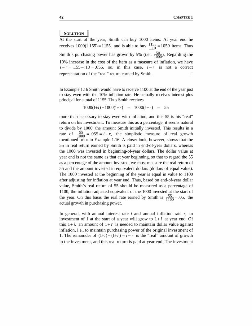
SOLUTION At the start of the year, Smith can buy 1000 items. At year end he receives 1000(1.155) 1155,= and is able to buy 1155

1.10 1050= items. Thus

Smith’s purchasing power has grown by 5% (i.e., 501000). Regarding the

10% increase in the cost of the item as a measure of inflation, we have .155 .10 .055,i r− = − = so, in this case, i r− is not a correct

representation of the “real” return earned by Smith. In Example 1.16 Smith would have to receive 1100 at the end of the year just to stay even with the 10% inflation rate. He actually receives interest plus principal for a total of 1155. Thus Smith receives

1000(1 ) 1000(1 ) 1000( ) 55i r i r+ − + = − =

more than necessary to stay even with inflation, and this 55 is his “real” return on his investment. To measure this as a percentage, it seems natural to divide by 1000, the amount Smith initially invested. This results in a rate of 55

1000 .055 ,i r= = − the simplistic measure of real growth mentioned prior to Example 1.16. A closer look, however, shows that the 55 in real return earned by Smith is paid in end-of-year dollars, whereas the 1000 was invested in beginning-of-year dollars. The dollar value at year end is not the same as that at year beginning, so that to regard the 55 as a percentage of the amount invested, we must measure the real return of 55 and the amount invested in equivalent dollars (dollars of equal value). The 1000 invested at the beginning of the year is equal in value to 1100 after adjusting for inflation at year end. Thus, based on end-of-year dollar value, Smith’s real return of 55 should be measured as a percentage of 1100, the inflation-adjusted equivalent of the 1000 invested at the start of the year. On this basis the real rate earned by Smith is 55

1100 .05,= the actual growth in purchasing power. In general, with annual interest rate i and annual inflation rate r, an investment of 1 at the start of a year will grow to 1 i+ at year end. Of this 1 ,i+ an amount of 1 r+ is needed to maintain dollar value against inflation, i.e., to maintain purchasing power of the original investment of 1. The remainder of (1 ) (1 )i r i r+ − + = − is the “real” amount of growth in the investment, and this real return is paid at year end. The investment

Copyright © 1995 - 2008, Bank

of Canada. Permission is granted

to reproduce or cite portions

herein, if attribution is given to

the Bank of Canada. Contact us.

Read our privacy statement.

Implementation of Fixed Announcement Dates:

Information paper: A new system of fixed dates for announcing changes to the Bank Rate (2000)

Consultation results: Summary of consultation results

Monetary policy implementation/LVTS-related Operating band, settlement balances, special operations, etc.

24 April 2007 4.25 ---

More data

Page 2 of 2Key interest rate: target for the overnight rate- Monetary Policy- Bank of Canada

22/09/2008http://www.bankofcanada.ca/en/monetary/target.html

68 CHAPTER 2

Chapter. There is a collection of computer spreadsheet illustrations, including illustrations of annuity calculations available at the website of the publisher of this book, www.actexmadriver.com. The presentation here emphasizes understanding the algebraic relationships involved in annuity valuation.

A key algebraic relationship used in valuing a series of payments is the familiar geometric series summation formula

1 1

2 1 11 .1 1

k kk x xx x x

x x

+ +− −+ + + + = =

− − (2.1)

This is illustrated in the following example.

EXAMPLE 2.1 (Accumulation of a level payment annuity)

The federal government sends Smith a family allowance payment of $30 every month for Smith’s child. Smith deposits the payments in a bank account on the last day of each month. The account earns interest at the annual rate of 9% compounded monthly and payable on the last day of each month, on the minimum monthly balance. If the first payment is deposited on May 31, 1998, what is the account balance on December 31, 2009, including the payment just made?

SOLUTION The one-month compound interest rate is .0075.j = The balance in the account on June 30, 1998, including the payment just deposited and the accumulated value of the May 31 deposit is

2 30(1 ) 30 30[(1 ) 1].C j j= + + = + + The balance on July 31, 1998 is

[ ] 2

3 2 (1 ) 30 (1 ) 1 (1 ) 30 30 (1 ) (1 ) 1 .C C j j j j j⎡ ⎤= + + = + + + + = + + + +⎣ ⎦ Continuing in this way we see that the balance just after the thm deposit is

1 230 (1 ) (1 ) (1 ) 1 ,mmC j j j−⎡ ⎤= + + + + + + +⎣ ⎦ the accumulation of those

VALUATION OF ANNUITIES 69

first m deposits. The balance on December 31, 2009, just after the 140th deposit is

139 13830 (1 ) (1 ) (1 ) 1j j j⎡ ⎤+ + + + + + +⎣ ⎦

140 140(1 ) 1 (1.0075) 130 30 7385.91.(1 ) 1 .0075

jj

⎡ ⎤ ⎡ ⎤+ − −= = =⎢ ⎥ ⎢ ⎥+ − ⎣ ⎦⎣ ⎦

We have applied the geometric series formula in the equation above. The following line diagram illustrates the accumulation in the account from one deposit to the next. May 31 June 30 July 31

30

30(1 )

30j+

+

230(1 )30(1 )

30

jj

++

+

FIGURE 2.1 2.1 LEVEL PAYMENT ANNUITIES

2.1.1 ACCUMULATED VALUE OF AN ANNUITY

In Example 2.1, the expression for the aggregate accumulated value on December 31, 2009 is

139 13830 (1 ) (1 ) (1 ) 1j j j⎡ ⎤+ + + + + + +⎣ ⎦ 139 13830(1 ) 30(1 ) 30(1 ) 30.j j j= + + + + + + +

The right hand side of the equation is the sum of the accumulated values of the individual deposits. 13930(1 )j+ is the accumulated value on December 31, 2009 of the deposit made on May 31, 1998, 13830(1 )j+ is the accumulated value on December 31, 2009 of the deposit made on June 30, 1998, and so on.

Course 2 48 May 2000

47. Jim began saving money for his retirement by making monthly deposits of 200 into

a fund earning 6% interest compounded monthly. The first deposit occurred on

January 1, 1985 .

Jim became unemployed and missed making deposits 60 through 72 . He then

continued making monthly deposits of 200 .

How much did Jim accumulate in his fund on December 31, 1999 ?

(A) 53,572

(B) 53,715

(C) 53,840

(D) 53,966

(E) 54,184

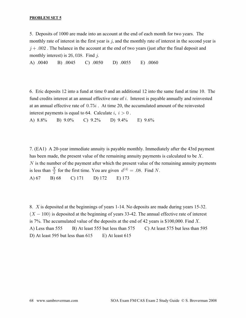
PROBLEM SET 5

68 www.sambroverman.com SOA Exam FM/CAS Exam 2 Study Guide © S. Broverman 2008

5. Deposits of 1000 are made into an account at the end of each month for two years. Themonthly rate of interest in the first year is , and the monthly rate of interest in the second year is

. The balance in the account at the end of two years (just after the final deposit andmonthly interest) is . Find .A) .0040 B) .0045 C) .0050 D) .0055 E) .0060

6. Eric deposits 12 into a fund at time 0 and an additional 12 into the same fund at time 10. Thefund credits interest at an annual effective rate of . Interest is payable annually and reinvestedat an annual effective rate of . At time 20, the accumulated amount of the reinvestedinterest payments is equal to 64. Calculate , .A) 8.8% B) 9.0% C) 9.2% D) 9.4% E) 9.6%

7. (EA1) A 20-year immediate annuity is payable monthly. Immediately after the 43rd paymenthas been made, the present value of the remaining annuity payments is calculated to be .

is the number of the payment after which the present value of the remaining annuity paymentsis less than for the first time. You are given . Find .A) 67 B) 68 C) 171 D) 172 E) 173

8. is deposited at the beginnings of years 1-14. No deposits are made during years 15-32. is deposited at the beginning of years 33-42. The annual effective rate of interest

is 7%. The accumulated value of the deposits at the end of 42 years is $100,000. Find .A) Less than 555 B) At least 555 but less than 575 C) At least 575 but less than 595D) At least 595 but less than 615 E) At least 615

78 CHAPTER 2

0 1 2 1n− n 1n+ 2n+ n k+ 1 1 1 1 1 1 1

1 22(1 )k

n i k is i s↑

⋅ + +

Note that if the interest rate is level over the n k+ periods, so that

2 1,i i= then Equation 2.5 is the same as the expression in (d). This method can be extended to situations in which the interest rate changes more than once during the term of the annuity. The relationship in Equation 2.5 can also be used to find the accumulated value of an annuity for which the payment amount changes during the course of the annuity. The following example illustrates this point.

EXAMPLE 2.5

(Annuity whose payment amount changes during annuity term) Suppose that 10 monthly payments of 50 each are followed by 14 monthly payments of 75 each. If interest is at an effective monthly rate of 1%, what is the accumulated value of the series at the time of the final payment?

SOLUTION Using the same technique as in Example 2.3 for finding the accumulated value of an annuity some time after the final payment, at the time 24 (months), the accumulated value of the first 10 payments is

1410 .0150 (1.01) 601.30.s ⋅ =

The value of the final 14 payments, also valued at time 24 is

14 .0175 1,121.06.s =

The total accumulated value at time 24 is 1722.36. There is an alternative way of approaching this situation. Note in Figure 2.4 below that the original (non-level) sequence of payments can be decomposed into two separate level sequences of payments, both of which end at time 24.

VALUATION OF ANNUITIES 79

Time 0 1 2 10 11 12 24 Original Series 50 50 50 75 75 75 New Series 1 50 50 50 50 50 50 New Series 2 25 25 25

FIGURE 2.4

The associated EXCEL files found at the ACTEX website include a general recursive procedure for finding the accumulated value of an annuity which has payments and interest rates that change from one year to the next. The accumulated value (at time 24) of the alternate form of the series is

24 .01 14 .0150 25 1,348.67 373.69 1,722.36.s s+ = + =

2.1.2 PRESENT VALUE OF AN ANNUITY

The discussion above has been concerned with formulating and calculating the accumulated value of a series of payments at the time the payments end or some time after the payments end. We now consider the present value of an annuity.

EXAMPLE 2.6 (Present value of a series of payments)

Smith’s grandchild will begin a four year college program in one year. Smith wishes to open a bank account with a single deposit today so that her grandchild can withdraw $1000 per year for four years from the account, starting one year from now. The account has an effective annual interest rate of 6% and the deposit is calculated so that the account balance will be reduced to 0 when the fourth withdrawal is made four years from now. Determine the amount of the deposit Smith makes today.

SOLUTION Suppose that the amount of the initial deposit is X. If we track the account balance after each withdrawal, we see the following: Balance after 1st withdrawal:

(1.06) 1000X −