UNIVERSITÀ DEGLI STUDI DI NAPOLI “FEDERICO II”

FACOLTÀ DI ECONOMIA

DOTTORATO IN MATEMATICA PER L’ANALISI ECONOMICA E LA FINANZA

XXIII – CICLO

Coupon Bonds and Liquidation Triggers: A Real Option Approach

Program Coordinator: Prof. Dr. Rosa Cocozza

Supervisor: Prof. Dr. Marco Pagano

Giovanni Piccolo

Academic year: 2012 – ‘13

1

to my parents and my sister and …

…to SRSLC

2

CONTENTS

INTRODUCTION 5

US Bankruptcy Code 7

Chapter 7 7

Chapter 11 8

Summary 9

Conclusion 9

CHAPTER 1 11

1. Literature review 11

1.1 Real Option Literature 12

1.2 Structural Models literature 15

1.2.1 Default at maturity 15

1.2.2 Market Value and distress threshold 16

1.2.3 Not Immediate Liquidation 19

1.2.4 Renegotiations 22

1.2.5 Recent Evolution 24

1.2.6 Comparison with empirical data 26

CHAPTER 2 – A Real Option Model with two ZCBs 30

2 Brief introduction 30

2.1 Structural Model 31

2.1.1 Model assumptions 32

2.1.1.1 Asset Value 32

2.1.1.2 Debt 33

2.1.1.3 Liquidation Costs 33

2.1.1.4 The threshold level 34

2.1.1.5 Random Variables 34

2.2 The valuation of corporate securities 35

2.2.1 Equity Value 35

2.2.2 Senior Bond Value 36

2.2.3 Junior Bond Value 37

2.3 Default Probabilities 39

2.4 Recovery Rate 40

2.5 Yield to maturity and Credit Spread 40

2.6 Numerical implementation 41

2.7 Parameters’ choice 41

2.8 Results vs. Empirical data 43

3

2.8.1 Cumulative DPS 44

2.8.2 Recovery Rate 45

2.8.3 Yield Spread 45

2.8.4 Empirical cumulative DPs vs. old models 46

2.9 Hypothetical country 47

2.10 Sensitivity analysis 48

2.10.1 Grace period (d) 48

2.10.2 Volatility (sigma) 50

2.10.3 The percentage of Senior Bond on the Total Debt 52

2.10.4 Dividend yield (delta) 53

2.10.5 Liquidation Costs 55

2.10.6 Leverage Ratio 56

2.10.7 Threshold's parameter (Omega) 58

2.10.8 Free-risk Rate (r) 60

2.11 Conclusion 61

CHAPTER 3 – A Real Option Model with a Junior Coupon Bond 64

3 Brief Introduction 64

3.1 Structural Model 65

3.1.1 Model assumptions 66

3.1.1.1 Asset Value 66

3.1.1.2 Debt 66

3.1.1.3 Liquidation Costs 66

3.1.1.4 The threshold level 67

3.1.1.5 Random Variables 67

3.2 The valuation of corporate securities 68

3.2.1 Equity Value 68

3.2.2 Senior Debt 69

3.2.3 Junior Debt 70

3.3 Benchmark 71

3.4 Numerical implementation 72

3.5 Parameters’ choice 72

3.6 Results 73

3.6.1 Cumulative DPS 74

3.6.2 Recovery Rate 75

3.6.3 Yield Spread 75

3.6.4 Empirical cumulative DPs vs. old models 75

3.7 Hypothetical country 77

3.8 Sensitivity analysis 78

3.8.1 Grace period (g) 78

3.8.2 Volatility (sigma) 80

3.8.3 The percentage of Senior Bond on the Total Debt 82

4

3.8.4 Dividend yield (delta) 83

3.8.5 Liquidation Costs 85

3.8.6 Leverage Ratio 86

3.8.7 Threshold's parameter (Omega) 88

3.8.8 Free-risk Rate (r) 89

3.9 Conclusion 91

Appendix A – A Real Option Model with a Senior Coupon Bond 94

A. Brief Introduction 94

A.1 Structural Model 94

A.2 The valuation of corporate securities 94

A.2.1 Equity Value 95

A.2.2 Senior Debt 95

A.2.3 Junior Debt 96

A.3 Benchmark 98

A.4 Numerical implementation 98

A.5 Parameters’ choice 98

A.6 Results 99

A.6.1 Cumulative DPS 100

A.6.2 Recovery Rate 100

A.6.3 Yield Spread 101

A.6.4 Empirical cumulative DPs vs. old models 101

A.7 Hypothetical country 102

A.8 Sensitivity analysis 103

A.8.1 Grace period (d) 104

A.8.2 Volatility (sigma) 105

A.8.4 Dividend yield (delta) 108

A.8.5 Liquidation Costs 110

A.8.6 Leverage Ratio 111

A.8.7 Threshold's parameter (Omega) 112

A.8.8 Free-risk Rate (r) 114

A.9 Conclusion 115

References 116

5

INTRODUCTION

Numerous empiric studies show that the interval between the beginning of financial distress

and liquidation in the United States is included between 1 and 3 years (this gap is different

around the world but it exists everywhere). However, many pricing models of corporate

securities have the assumption that financial distress or default lead to immediate liquidation

of firm assets.

These models assume that the liquidation or reorganization occurs when a defined bankruptcy

trigger is met. This assumption is supported by common covenants, which give the debt-

holders the right to ask for liquidation/reorganization if the firm asset’s value falls below a

pre-defined threshold.

I implement a structural model in which liquidation starts only if a time variable exceed a pre-

defined grace period, in order to capture the effects of the time gap between the beginning of

the financial distress and the moment of liquidation on cumulative default probabilities,

recovery rate, yield spreads and on the corporate securities value.

In practice, I build a real option model in which the asset value is exogenous, there are a

threshold barrier, a grace period and the firm’s capital structure is complex. Indeed, there are

two types of debts: a junior debt and a senior debt. Both bonds could be Zero Coupon Bond or

Coupon Bond with maturity equal to 10 years.

The mechanism of the model take into account (through the presence of a pre-defined grace

period) the characteristic of the US bankruptcy Code and reproduce the Chapter 7 case (I

hypothesize that my representative B-rated firm can not continue its business when the asset

value stay for 1 year below the threshold barrier).

The contribution of this approach is that I consider the presence of coupons and liquidation

cost and at the same time the main common funding forms: equity, senior debt and junior

6

debt. Other approach/papers, that consider the existence of the grace period, do not consider

liquidation cost and hypothesize the presence of a very simple capital structure with equity

and one Zero Coupon Bond. In addition, I use parameters’ value equal to those found in

literature and, consequently, I do not apply any type of calibration approach.

Therefore, I can compare cumulative default probabilities, recovery rate and yield spread

computed through my approach with those empirically found, in order to understand the

reliability of my model. At the same time, solving the model numerically, I can make a

comparative statics and, consequently, I can evaluate how the parameters of the model affect

the probability of default, the recovery rate, the yield spread and the value of the assets.

In order to evaluate the reliability of my framework, I use as benchmark the average

cumulative default frequencies for B-rated debt as function of horizon, as given by Moody's

(2011), the recovery rate found by Altman & Kishore (1996), the average yield spread over

treasury bond of similar maturity for B-rated bonds, as reported by Huang & Huang (2003).

In Chapter 2, where I present a first version of my model in which I introduce liquidation cost,

two debts and the grace period, the results that I get are mixed. Indeed, my cumulative default

probabilities are lower than empirical data, my recovery rate is close to Huang & Huang

(2003) data, while the recovery rate is almost coincident with the value found empirically. At

the same time, I show that old models (hit and default) fail. In fact, using these models, I get a

good approximation of cumulative default probabilities, while the recovery rate is very far

from empirical value.

When I introduce coupons in Chapter 3 (and in Appendix A), I obtain results very satisfying,

since the evolution of my cumulative default probabilities is compliant with empirical default

probabilities and my recovery rate and my yield spread are almost coincident with those found

in literature. I do not achieve the same outcomes if I adapt old models to my framework.

7

Indeed, if I include coupons, liquidation cost and two type of bond in old structure, the results

are completely different from those empirically computed.

In summary: I am able to capture some stylized facts (such as cumulative Dps, recovery rate

and yield spreads); I do that using real ingredients, since I use parameters’ value (volatility,

risk free rate, dividend yield, grace period, etc.) found in a couple of empirical research; and I

could assert that the presence of grace period and the introduction of coupons are crucial

ingredients for matching empirical data.

US Bankruptcy Code

The procedural aspects of the bankruptcy process are governed by the Federal Rules of

Bankruptcy Procedure and local rules of each bankruptcy court. The Bankruptcy Code and

Bankruptcy Rules (and local rules) set forth the formal legal procedures for dealing with the

debt problems of individuals and businesses.

Indeed, six basic types of bankruptcy cases are provided for under the Bankruptcy Code, but

only two of these filings are available to corporations: Chapter 7 and Chapter 11.

Chapter 7

In Chapter 7, a Court-appointed trustee liquidates the firm’s assets and uses the proceeds to

pay the holders of claims (creditors) in accordance with the provisions of the Bankruptcy

Code. Company stops all operations and goes completely out of business. Indeed, some firms

are so far in debt or have other problems so serious that can not continue their business

operations. Administrative and legal expenses are paid first, and the remainder goes to

creditors.

8

Secured creditors will have their collateral returned to them. If the value of the collateral is not

sufficient to repay them in full, they will be grouped with other unsecured creditors for the rest

of their claim.

Bondholders and other unsecured creditors will be notified of the Chapter 7, and should file a

claim in case there is money left for them to receive a payment.

Stockholders do not have to be notified of the Chapter 7 case because they generally do not

receive anything in return for their investment. In the unlikely event that creditors are paid in

full, stockholders will be notified and given an opportunity to file claims.

Chapter 11

Chapter 11 is used by corporations that desire to continue operating business and repay

creditors trough a court-approved plan of reorganization. In this case: 1) the creditor may seek

an adjustment of debts, either by reducing the debt or by extending the time for repayment, or

may seek a more comprehensive reorganization; 2) Management continues to run the day-to-

day business operations but all significant business decisions must be approved by a

bankruptcy court.

In practice, the steps of this procedure are the following:

1) Company prepares a plan of reorganization and the U.S. Trustee, the bankruptcy arm of the

Justice Department will appoint one or more committees to represent the different

stakeholders in working with the company to develop this plan;

2) The plan must be accepted by creditors, bondholders and stockholders;

3) Company prepares a disclosure statement and reorganization plan and files it with the

court;

4) SEC (Security and Exchange Commission) reviews the disclosure statement to be sure it is

complete;

9

5) the bankruptcy court confirms the plan confirmation.

Summary

When a firm is in bankruptcy there are four primary groups that could influence the future of

this firm: Managers, Shareholders, unsecured Creditors1 and secured Creditors.

Usually, Managers, Shareholders and unsecured Creditors prefer reorganization over

liquidation, while secured Creditors could be harmed by reorganization.

Whit the 1978 Act, creditors have the possibility to propose their own plan of reorganization

after managers have had 180 days to suggest their plan. The problem is that each class of

creditors must be in favour of this plan. In addition, shareholders could vote for this approval

if their claims are impaired.

Conclusion

It is demonstrated that old models (or hit and default models), very popular in 1980s and

1990s, are not able to match the empirical data, even if they are naïf models. Indeed, in a

couple of research it was used a calibration approach in order to get results similar to

empirical outcomes.

In addition, it is verified that in reality default and liquidation are distinct events and the

default threshold isn’t an absorbing barrier.

Therefore, I build a more complex and realistic model with less degrees of freedom, in which

I take into account a grace period in order to study the economic implications of this element.

Using this approach and adding coupons bonds instead of ZCB, I am able to fit empirical data

(cumulative default probabilities, recovery rate and yield spreads) without any type of

1 Employees with past wages due and customers with deposits have a priority over other unsecured creditors.

10

calibration. In fact, I capture these stylized facts with real ingredients, since I choose the

parameters’ value found in a couple of empirical research.

I think that is possible to extend this model considering a liquidation state variable that is

dependent of the severity of distress or different dynamics of risk–free rate or introducing

other parameters (such as taxes).

11

CHAPTER 1

1. Literature review

In much of the continuous-time debt pricing literature, it has typically been assumed that

default is tantamount to liquidation.

In reality, most of the companies which default go into a period of reorganization and may or

may not be liquidated.

Indeed, using US data, Gilson, John, & Lang (1990) investigate the incentives of financially

distressed firms to restructure their debt privately rather than through formal bankruptcy. In

their sample of financially distressed companies, about half successfully restructure their debt

outside of Chapter 11. They find that only about 5% of the bankruptcies in Chapter 11 are

converted into Chapter 7 liquidations.

Using data on distressed UK companies, Franks & Sussman (2005) also find that: the typical

debt structure is close to a corner solution, with the liquidation rights almost entirely

concentrated in the hands of the main bank; while the banks’ typical response to distress is an

attempt to rescue the firm (rather than liquidate it automatically), they are very tough in their

bargaining with the distressed firm; concentrating the liquidation rights helps to resolve co-

ordination failures.

In addition, numerous empiric studies show that the interval between the beginning of

financial distress and liquidation in the United States is included between 1 and 3 years (this

gap is different around the world but it exists everywhere).

In fact, Covitz, Han & Wilson (2006) find that time in default is significantly related to

whether the bankruptcy is triggered by litigation, the industry and macroeconomic conditions

at the time of default, and the change in these conditions over the duration of the default.

They, in addition, show that there has been a significant decline in the length of time spent in

12

default for US public companies, for approximately 36 months in late 1980s to 12 months

between 1993 and 2002;

Thorburn (2000) provides some first, large-sample evidence on the Swedish auction

bankruptcy system. Compared to U.S. Chapter 11 cases, the small-firm bankruptcy auctions

examined here are substantially quicker (2.5 months), have lower costs, and avoid deviations

from absolute priority. Three-quarters of the firms are auctioned as going concerns, which is

similar to Chapter 11 survival rates. Moreover, based on market values, creditors in going-

concern auctions recover a similar fraction of face value as creditors of much larger firms in

Chapter 11 reorganizations. The evidence presented suggests that the auction bankruptcy

system is a surprisingly efficient restructuring mechanism for small firms.

Recently, some debt pricing models have therefore attempted to separate the notions of default

and liquidation and/or take into account this time gap between the beginning of the financial

distress and the moment of liquidation.

The rest of the chapter is structured as follow. The next paragraph describes real option

literature. Paragraph 1.2 shows the evolution of the theoretical pricing (structural) models of

corporate securities from Black & Scholes (1973) and Merton (1974) to Bruche (2011), that

are based on different type of liquidation hypothesis. Finally I present some empirical studies

used to test the reliability of these structural models.

1.1 Real Option Literature

In the last few decades it has been recorded in the financial markets a significant growth in

both volume and complexity of the contracts that are traded in the over-the-counter market.

Black & Scholes (1973) derived a theoretical valuation formula for options based on the

principle that “it should not be possible to make sure profits by creating portfolios of long and

13

short positions in options and their underlying stocks” if options are correctly priced in the

market.

Black & Scholes model is still widely used for options pricing, even though a couple of

empirical papers have shown that the model does not explain the underlying asset price

process.

A large number of models have been proposed to address the empirical weakness of the

classic Black-Scholes approach. These extended models have been developed though three

dimensions: univariate diffusion models, Stochastic volatility models and Jump models.

The univariate diffusion models are models in which it is relaxed the assumption of Geometric

Brownian motion. In this category are included: the constant elasticity of variance models of

Cox & Ross (1976) and Cox & Rubinstein (1985); the leverage models of Gesken (1979) &

Rubinstein (1983); and the implied binomial and trinomial trees models such as Derman &

Kani (1994) and Dupire (1994). At the beginning univariate diffusion were used in order to

capture time-varying volatility and the leverage effect in a simple fashion. Then, these models

were built to match observed cross-sectional option pricing patterns at any instant, in order to

price over the counter exotic options.

Stochastic volatility models in which the instantaneous volatility of assets returns evolve

stochastically over time as a diffusion process (Hull & White, 1987), as a regime switching

process (in Naik, 1993) or as jump diffusion process (in Duffie, Pan & Singleton, 2000). The

advantage of adopting stochastic volatility models is that these models are consistent with the

stochastic and mean-reverting evolution of implicit standard deviations.

Jump models relax the diffusion assumption for asset prices such as Merton (1976) and Bates

(1991). These models were used to match volatility smiles2 and smirks3.

2 A plot of implied volatility vs. strike price will form an U-shaped curve similar to the shape of a smile. 3 Implied volatility for options at the lower strikes are higher than the implied volatility at higher strikes.

14

Other models have combined features of these three approaches. Stochastic generalizations of

binomial tree models are surveyed by Skiadopoulos (2000) while the affine class of

distributional models creates a structure that nests particular specifications of the stochastic

volatility and jump approaches.

All these models are more realistic than the Black and Scholes model. However, it is not sure

if they improve pricing correctness and hedging performance. Indeed, each model relaxes

several hypothesis of the Black and Scholes model, but the extra risk introduced raises the

issue of how to price these risk.

In the 1980s it was very complicated to test the different approaches, because option data were

not available until the introduction of option trading on centralized exchanges.

The introduction of some developments such as the Monte Carlo approach of Scott (1987), the

higher dimensional finite difference approach of Wiggins (1987) and, principally, the Fourier

inversion approaches of Stein & Stein (1991) and Heston, (1993), have facilitated the

comparison between alternative option pricing models.

There are, therefore, a couple of empirical papers that test the performance of option pricing

model, including Bakshi, Cao & Chen (1997 and 2000), Bates (1996 and 2000) and Dumas,

Fleming & Whaley (1998), among others.

Empirical test are realized in this way: parameters of the model are estimated so that the

model prices for some european options match the price that are observed in the market at a

specific time. The resulting model is used to price other options later and then these prices are

compared with those observed from the market.

However, Bakshi, Cao & Chen (1997) show that instantaneous option price evolution is not

fully captured by underlying asset price movements, precluding the riskless hedging predicted

by univariate diffusion models.

15

Bates (2000) points out that the standard assumption of independent and identically

distributed returns in jump model implies these models converge towards BS model option

prices at longer maturities, in contrast to the still pronounced volatility smiles and smirks (or

reverse skew) at those maturities.

Bakshi, Cao & Chen (2000) find that adding jumps or stochastic interest rate does not improve

the unconstrained stochastic volatility model’s assessments of how to hedge option price

movements. At the same, it is demonstrated that unconstrained stochastic volatility models

price options better after jumps are added.

1.2 Structural Models literature

The evolution of the structural models from Black & Scholes (1973) and Merton (1974) to

Bruche (2011) is presented here.

1.2.1 Default at maturity

In order to determine the value of corporate securities is essential the modelling of default.

The classic approach is based on the idea that default is possible in the event that the total

value of the firm is less than total amount of the debt.

For the first time, in fact, Black & Scholes (1973) pointed out that equity value is similar to

the price of European call options, with a strike price equal to the total value of the debt at

maturity.

They build a model in which there is a company that had common stock and bonds

outstanding. In addition, they suppose that: bonds are zero coupon bonds, giving the holder

the right to a fixed sum of money, if the firm can pay it, with a maturity of 10 years; bonds

contain no restrictions on the company except a limitation that the company can not pay any

16

dividends; the company plans to sell all assets it holds at the end of 10 years, pay off the bond

holders if possible, and pay any remaining money to the stockholders.

In according with this model: the bondholders own the company’s asset, while the

stockholders have an option for buying the asset back; and the total value of equity at the

maturity is equal to the maximum between zero and the difference between value of the

company’s asset minus the face value of the bonds.

At the same time, Merton (1974) developed a theory for pricing bonds when there is a

significant probability of default, using the same hypothesis: “On the maturity date T, the firm

must either pay the promised payment of B (total debt) to the debtholders or else the current

equity will be valueless”.

In practice, the value of corporate debt depends on the required rate of return on riskless, the

various provisions and restrictions contained in the agreement and the probability that the firm

will be unable to satisfy some or all of the indenture requirements.

Finally, Galai & Masulis (1976) combine the option pricing model with the capital asset

pricing model in order to find a more complete model of security pricing. They show that this

combination of models leads to a number of insights regarding stock risk and changes in

corporate asset structure and capital structure.

In these models there is a common assumption that defaults and financial distress bring to

immediate liquidation of firm assets.

1.2.2 Market Value and distress threshold

Black & Cox (1976), for the first time, introduced the effects of safety covenants on the value

and behaviour of the firm securities. In particular, they considered the possibility of

bankruptcy at any time or rather the hypothesis for which if the firm’s value drops to a

17

specified level, that is variable over time, then the bondholders could force the firm into

bankruptcy and, consequently, get the ownership of the assets.

The authors also took into account the subordination of the claims of one class of bondholders

(junior debt) to those of a second class (senior bond) and treated these two different type of

assets as two options with different exercise prices.

Brennan & Schwartz (1978), on the other hand, studied the effects of corporate income taxes

on the relationship between capital structure and valuation. They showed that the issue of

additional debt have two effects on the value of the firm and, in particular, it increases the tax

savings to be enjoyed so long as the firm survives and reduces the probability of the firm’s

survival for any given period.

In order to solve the model, they assumed (boundary condition) that the firm files for

bankruptcy at any time if the value of its assets is less than the par value of outstanding bonds.

In addition, Mello & Parsons (1992) show how to adapt a contingent claims model to reflect

the incentive effects of the capital structure and to measure the agency costs of debt. They

suppose that the value of the firm is an endogenous function of an underlying stochastic

variable describing the firm’s product market and of the management’s choice of operating

and investment decisions.

Also in this model there is the hypothesis that default leads to an immediate liquidation of ths

firm’s assets.

In order to compute the Corporate Debt Value and define Optimal Capital Structure, Leland

(1994) considered two different approaches the case in which bankruptcy is determined

endogenously; or the case in which debt remains outstanding without time limit unless

bankruptcy is triggered by the value of the firm's assets falling beneath the principal value of

debt. This latter situation could be representative of a situation in which there is a long term

debt with a protective covenant stipulating that the asset value of the firm is bigger than the

18

principal value of the debt; or a continuously renewable line of credit with fixed interest rate

and fixed amount of borrowing and at each instant the debt will be rolled over if the value of

the assets is sufficient to repay the loan’s principal (if not there is bankruptcy).

In this framework, however, Leland assume that the face value of debt remains static through

time and that if bankruptcy occurs, a fraction 0 < a < 1 of value will be lost to bankruptcy

costs, leaving debtholders with value (1 - a)*V and stockholders with nothing.

Longstaff & Schwartz (1995), moreover, for valuing risky corporate debt, developed a model

that incorporates both default and interest rate risk, allows for deviations from strict absolute

priority rules if the firm defaults and, as in Black and Cox (1976), includes a threshold value

K for the firm at which financial distress occurs. If the asset value is greater than K, the firm

continues to be able to meet its contractual obligations. If the asset value reaches K there is a

financial distress and some form of corporate restructuring takes place.

Ericsson & Reneby, (2001) showed that many corporate securities can be viewed as portfolio

of three basic claims (with simple valuation formulae): a down-and-out call option, a down-

and-out binary option and a unit down-and-in claim. They assumed that default occurs at any

time prior to maturity if the value of the assets falls below a constant or at debt maturity if the

value of the assets is smaller than the total amount of debt.

The second case is redundant when, as in Black and Cox and in Leland, the models are

characterized by a stationary (perpetual) capital structure.

Then, Leland & Toft (1996) develop a model of optimal leverage and risky corporate bond

prices for arbitrary debt maturity. Bankruptcy is determined endogenously and will depend on

the maturity of debt as well as its amount. Both value and flow conditions that characterize the

bankruptcy point are presented. They show that bankruptcy can occur at asset values that may

be either lower or higher than the principal value of debt. And a cash flow shortfall relative to

19

required debt service payments need not result in default-it may be optimal for equity holders

to raise further funds to avoid bankruptcy.

In order to estimate the tax advantage to debt and to determine optimal capital structure

policy, Goldstein, Ju & Leland (2001) develop a theoretical model that provide a state variable

which is invariant under capital structure change and account for cash payouts, since payout

affects the probability of future bankruptcy.

They suppose, anyway, that the management chooses the bankruptcy level in the best interest

of the equityholders and that default brings to an immediate liquidation of the asset.

Finally, Morellec, (2001) investigates the impact of asset liquidity on the values of corporate

securities and the firm’s financing decisions. The model endogenously determines both the

default threshold and the sales curve that maximize equity value. Because of the limited

liability principle, shareholders have the option to default on their obligations. The optimal

exercise policy for this option is to default when the firm has negative economic net worth.

1.2.3 Not Immediate Liquidation

Recent theoretical works on capital structure and securities valuation suggest that liquidation

happens only if the asset’s value are smaller than a particular value (distress threshold) for an

interval exceeding a pre-defined grace period.

For example Mella-Barral (1999) assumes that liquidity problems do not have any influence

on the default point as the debtors can keep on issuing equity to avoid a default. Subsequently

in his model, default is endogenous and is the point where it is optimal for the debtors to

irreversibly exchange their current claim for a residual claim which they will get on

bankruptcy.

Hege & Merra-Barral (2000) extend Mella-Barral (1999) by taking into account multiple

creditors.

20

Then, Fan & Sundaresan (2000) suggest that when the firm is in default, borrowers stop

making the contractual coupon and start servicing the debt strategically until the firm’s asset

value goes back above the distress threshold. They show that Bankruptcies are often resolved

using exchange offers of different types, such as delayed or missed interest or principal

payments, extension of maturity, debt-equity swap, debt holidays, etc. Essentially all these

distressed exchanges and delayed payments can be considered for them as a value

redistribution between equity and debt holders. This assumption is based on Moody's

Investors Service (1998), where are analyzed all defaults during 1982-1997. This research

report that about half of long-term public bond defaults resulted in bankruptcy. Of the

defaults, 43% were accounted for by missed payments and 7% by distressed exchanges.

François & Morellec (2004), on the other hand, suppose that default can lead either to

liquidation of the firm’s assets or to renegotiation of the debt contract. In bankruptcy, the firm

incurs costs of financial distress, and the cash flows it generates are shared among

claimholders. Moreover, for firms that choose to renegotiate their claims under the court’s

protection, the default date is the starting point of a period during which the parties involved

in the process (the claimholders and the court) observe the evolution of the value of the firm’s

assets. The firm emerges from financial distress if the value of its assets shows signs of

recovery during the observation period. Otherwise, liquidation is pronounced at the end of the

period. Shareholders hold a Parisian down-and-out call option on the firm’s assets. That is,

shareholders have a residual claim on the cash flows generated by the firm’s assets unless the

value of these assets reaches the default threshold and remains below that threshold for the

exclusivity period. In practice, they hypothesize that there isn’t any liquidation (fig 1, Case 1),

if the value of the firm’s assets (V) dips below the threshold (K) and then bounces above this

value before the conclusion of the grace period (d),. The liquidation occurs only if the value of

the firm’s asset is below the threshold K for a period bigger than d (fig.1, Case 2).

21

Figure 1 – The liquidation criterion

d d

KCase 1 Case 2

d d

KCase 1 Case 2

d dd d

KCase 1 Case 2

Moraux (2004) consider the model developed by François and Morellec and show that under

this type of liquidation procedure, debtholders may never receive coupons while the firm is

never liquidated. Indeed, every time the asset’s value goes above the default threshold, the

“distress clock” is reset to zero. In order to eliminate this problem, He consider the cumulative

excursion time below the default threshold, or better he assume that liquidation is declared

when the total time (cumulated) under the threshold is larger than d.

Finally, D.Galai, Raviv, & Wiener (2007) developed a model in which liquidation is driven

by a state variable that accumulates with time and the severity of distress. In particular, in this

model recent and severe distress events have a larger impact on the decision to liquidate a

firm’s asset, while old distress events have a slight effect on the liquidation decision because

the nature of the firm could have been changed in this period. Instead, mild financial distress

does not lead to immediate liquidation.

22

1.2.4 Renegotiations

Debtholders, in practice, don’t force to liquidate the firm’s assets immediately when financial

distress arrives.

Bebchuk & Chang (1992) and Bebchuk (2002) show that when an insolvent company files for

reorganization, an “automatic stay” prevents debtholders from seizing assets until a

reorganization plan is adopted.

Indeed, for political and social considerations, bankruptcy laws favour firm continuation and,

in particular, it is possible to have an out-of-court renegotiations or a legal bankruptcy

protection, like Chapter 11 of the U.S. Bankruptcy Code or Concordato Preventivo of the

Italian legge fallimentare, that authorize to renegotiate outstanding debt.

In this latter case, the supervising court would convert the bankruptcy proceedings to a

Chapter 7 (liquidation of the firm’s asset), if there is no agreement on a reorganization plan

between Debtholders and Equityholders. Before this conversion, it is impossible for

debtholders to receive any value from the company unless they agree with the equityholders

on the division of the firm’s assets.

Out-of-court renegotiations

For the first time, Anderson & Sundaresan (1996) study the design and valuation of debt

contracts in a general dynamic setting under uncertainty. Their framework is an extensive

form game determined by the terms of a debt contract and applicable bankruptcy laws.

Debtholders and equityholders behave non-cooperatively and the firm’s reorganization

boundary is determined endogenously.

Mella-Barral & Perraudin (1997), on the other hand, consider endogenous bankruptcy and

they model the strategic behaviour of debtors. In their models, the debtors act strategically and

always try to pay as low a coupon as possible. In good times when the liquidation value of the

23

firm is high, the debtors will not pay lower than the contracted amount as they would realise

that it would then be in the creditors’ interest to reject their offer and liquidate the firm.

However, the debtors might underperform the debt contract even if the firm is not

experiencing any liquidity problems. They will do this when the liquidation value of the firm

is not sufficiently high and thus when subsequently it would be not in the creditors’ interest to

reject the offer. Thus in their models, the debtors might default continuously and they will

continue to do so until the creditors finally reject the offer. At this point the firm will be

liquidated.

In Anderson and Sundaresan’s model and Mella-Barral and Perraudin’s model, endogenous

bankruptcy point will in general be different from the default point.

Finally, Christensen, Flor, Lando & Miltersen, (2000) consider a dynamic model of the capital

structure of a firm with callable debt that takes into account that equity holders and debt

holders have a common interest in restructuring the firm’s capital structure in order to avoid

bankruptcy costs. Far away from the bankruptcy threat the equity holders use the call feature

of the debt to replace the existing debt in order to increase the tax advantage to debt. When the

bankruptcy threat is imminent, the equity holders propose a restructuring of the existing debt

in order to avoid bankruptcy. This proposal makes both debt holders and equity holders better

off and re-optimize the firm’s capital structure. Both the lower and upper restructuring

boundaries are derived endogenously by the equity holders’ incentive compatibility

constraints.

Renegotiation under Chapter 11

Franks & Torous (1989) and Longstaff (1990) develop contingent claims models that analyze

the impact of Chapter 11 on debt values.

24

In particular, Franks & Torous (1989) describe the rights of the debtor-in-possession in

Chapter 11. Chapter 11 provides the debtor-in-possession with a valuable option, and they

have shown how that option may be priced into risky debt. Using simulation, the authors have

compared the risk adjusted rates of interest with the option to enter Chapter 11 with the risk

adjusted rates without that option.

Longstaff (1990) derive a closed form expression for the price of calls and puts that are

extendible by either the option holder or the option writer and show that many types of

corporate reorganizations, such as Chapter 11 bankruptcy, can be viewed as the exercise of an

implicit extension privilege.

In these two papers, the authors model Chapter 11 as the right to extend (once) the maturity

date of the debt. The longer this extension privilege, the more valuable it is to shareholders

and hence the larger the credit spread on corporate debt.

1.2.5 Recent Evolution

Broadie, Chernov & Sundaresan (2007) build a model in which the firm may choose to default

(Chapter 11) prior to completely destroying the equity value. This decision may still lead to

liquidation (Chapter 7), or it may result in recovery from default. In order to have this

framework they introduce two endogenous threshold along with a grace period. The first

barrier lead to the Chapter 11 filing, and the second barrier determines the liquidation’s

decision. The company, however, is allowed to stay in Chapter 11 for no more than the

duration of a grace period d. If the company spends more time than d in default, or if the value

of unlevered assets reaches the second barrier, then the firm is liquidated and there are

proportional costs of Liquidation.

Carr & Wu (2008) assume that there is a default corridor. They suppose that the stock price

stays above a barrier B > 0 before default, but drops below a lower barrier A < B at default

25

and stays below A thereafter. They have, implicitly, the same dynamics for the asset value

(V). In practice, in this model Carr and Wu hypothesize that when the default occurs the asset

value decreases, due to the liquidation cost.

Naqvi, (2008) develops a continuous time asset pricing model of debt restructuring and values

equity and debt by taking into account the fact that in practice the default point differs from

the liquidation point. This separation allows him to delegate the liquidation decision to the

creditors whilst default is triggered by the managers. The study identifies an agency cost of

debt whereby the creditors liquidate the firm prematurely relative to the first best threshold. In

this model default occurs because of liquidity problems and the critical default point is

determined exogenously. Naqvi assume that debt service is met out of cash flows and that the

firm cannot issue additional equity or debt to avoid a default. This is not a very stringent

assumption as it might first appear. In practice, debt covenants frequently restrict the issue of

additional debt with senior or equal status. Similarly, loan indentures quite often forbid the

liquidation of firm’s assets by owners as this could potentially undermine collateral values.

Bruche & Naqvi (2010) develop a model where equityholders decide when to default while

bondholders choose when to liquidate. In practice, creditors do not liquidate the firm

immediately upon default and could accept reduced coupon payments. Only in case of

deterioration of firm’s fundamental, they decide to liquidate. In this framework, the time

between the default and the liquidation is not related to a particular grace period but is

completely random.

Bruche (2011) presents a continuos-time structural model where there is a liquidation of a

defaulting firms only if debtholders, coordinated or uncoordinated, attempt to enforce claim

against these firms. In the model, coordinated creditors can have incentives to liquidate

prematurely, in the sense that firm value would be higher if the firm was liquidated later.

Uncoordinated creditors care about payoffs in an asset grab game. If legal costs of grabbing

26

assets are low, they can have incentives to grab assets too early. Features of Chapter-7 type

bankruptcy codes that affect creditor coordination change the payoffs in the asset grab game

such that grabbing assets becomes less attractive, protecting debtors. This leads to later

liquidation. The level of debt has, anyway, an effect on when the firm is liquidated, both in the

case in which creditors are coordinated as well as in the case where creditors are

uncoordinated.

1.2.6 Comparison with empirical data

Jones, Mason & Rosenfeld (1984) show that the credit yield spreads predicted by Merton

(1974) are far below the empirically observed corporate Treasury yield spreads, but a couple

of authors point out that extensions of the Merton Model within the structural framework that

incorporate some realistic economic consideration can explain the observed yield spreads.

Anderson, Sundaresan & Tychon (1996) believe that incorporating strategic default by equity

holders who try to extract concessions from bond holders can explain why corporate-Treasury

credit spreads should be high.

Collin-Dufresne & Goldstein (2001) propose a structural model of default with stochastic

interest rate. This model is able to show that firms with good credit quality are likely to issue

more debt, which leads to credit that are comparable to the observed high yield spreads for

long-maturity bonds issued by such firm.

Duffie & Lando (2001) study the implications of imperfect information for term structures of

credit spreads on corporate bonds (short maturity bonds). With imperfect information about

the firm’s value credit spreads remain bounded away from zero as maturity goes to zero and

are higher than those generated with perfect information.

Zhou, (2001) develop a model that incorporates jump risk into the default process. Whit this

jump risk, a firm could default immediately because of a rapid drop in its value. He show that

27

his model explain a number of empirical regularities regarding default probabilities and

recovery rates and it is able to match the size of credit spreads on corporate bonds.

Cooper & Davydenko (2004) propose a method of extracting expected returns on debt and

equity from corporate bond spreads. In practice, They propose to predict expected default

losses on any corporate bond based on its yield spreads, given information on leverage, equity

volatility and equity risk premia. In line with historical default rates, Cooper and Davydenko

find that only a small fraction of the spread for highgrade debt is due to expected default loss.

For lower-grade debt, this component is larger, and their approach provides a method for

adjusting yields to give expected debt returns. They find that the expected default component

of the spread varies significantly within ratings categories, so using average figures for ratings

categories for individual companies may be misleading.

Valuation of the capacity of different structural model to forecast real data

Many papers evaluates the capacity of structural models to forecast default rates, yield spread

or cumulative default probabilities.

Huang and Huang (2003) show that several structural models make quite similar predictions

on yield spreads if each of the models is calibrated to match historical default loss experience

data. They conclude that additional factors (illiquidity and taxes) must be important in

explaining the difference between the empirically-observed yield spreads and the predicted

spreads. In addition, Huang and Huang point out that for investment grade bonds of all

maturities, credit risk accounts for only a small fraction of the observed corporate Treasury

yield spreads, while for junk bonds credit risk accounts for a much larger fraction of the

observed corporate Treasury yield spreads.

Then, Eom, Helwege, & Huang (2004) test five structural models of corporate bond pricing.

They find that all models have substantial spread prediction errors, but their errors differ

28

sharply in both sign and magnitude. In particular, the average error is a rather poor summary

of a model’s predictive power, as the dispersion of predicted spreads is quite large. All models

tend to generate extremely low spreads on bonds that the models consider safe and to generate

very high spreads on the bonds considered to be very risky.

Leland (2004), instead, compare structural models’ abilities to predict observed default rates

on corporate bonds (as reported by Moody’s, 2001). In particular, Leland focus on two sets of

structural model that have been widely used in academic and practical applications: those with

“exogenous default boundary” that reflects only the principal value of debt, and those with an

“endogenous default boundary” where default is chosen by management to maximize equity

value. He finds that both the endogenous and exogenous have under-predicted default

probabilities at shorter time horizons and fits reasonably well the default probabilities,

especially for longer time horizons.

The author obtains these results through the calibration of the models and, although this

exercise provides acceptable levels of volatility, the predicted default probabilities are very

sensitive to this variable.

In addition, Teixeria (2007) tests empirically the performance of three structural models of

corporate bond pricing (Merton, Leland and Fan and Sundaresan). He find that the first two

models overestimate bond prices, while Fan and Sundaresan model reveals an extremely good

performance. When considering the prediction of credit spreads, the three models

underestimate market spreads but, again, Fan and Sundaresan has a better performance.

Tarashev (2008) use firm-level data in order to evaluate the degree to which five structural

credit-risk models account for the level and intertemporal evolution of actual default rates. He

finds that probabilities of default implied by the models tend to match the level of default

rates. In addition, his models explain a substantial portion of the variability of default rates

over time.

29

Finally, Schaefer & Strebulaev (2008) study the ability of structural model to predict the

hedge ratios of corporate bonds against the equity of the underlying firm. They show that even

the simplest structural model is capable of capturing the extent to which a change in the value

of corporate assets affect the value of corporate debt.

30

CHAPTER 2 – A Real Option Model with two ZCBs

2 Brief introduction

In this chapter, I try to replicate some stylized fact. In particular, I seek to reproduce the trend

of cumulative default probabilities, recovery rate and yield spread for B-rated firm, building a

real option model.

I start from some classical structural models, but I introduce some elements that are able to

make more realistic this framework. Specifically, I take into account the difference between

liquidation and default through a grace period, the presence of more complex capital structure

(as in reality) and the existence of liquidation cost.

In addition, I use real ingredients since I use parameter’s value found in a couple of empirical

papers and, consequently, I do not have any type of calibration approach.

In the next chapter I will suppose also that one of the bond issued by the firm is a Coupon

Bond, while in this construction I assume that both Bonds are zero coupon bonds as in a

couple of classic structural models.

My framework, therefore, has less degree of freedom (versus old models) and it is

characterized by an empirical modeling/test of the grace period.

The results, here, are mixed. Indeed, I am not able to fit the evolution of cumulative default

probabilities, but I find a recovery rate that is very close to empirical data, while my yield

spread is not very far from empirical data.

I show, however, that also using classical structural model the results are not very satisfying,

because with these models it is possible to reproduce the trend of cumulative default

probabilities, but it is impossible to find value of recovery rate and of yield spreads that are

comparable to those empirically found.

31

It is interesting, finally, to point out that in chapter 3 my results will be really satisfying and,

therefore, I will show that the combination of the presence of a grace period and of coupons is

crucial for reaching these results.

2.1 Structural Model

I build a real option model to estimate the value of various corporate securities (Senior Debt,

Junior Debt and Equity) under a wide array of bankruptcy procedures. This type of model also

generates quantitative predictions of default probabilities (or expected default frequencies) for

bonds. I will use these cumulative Default Probabilities data in order to verity if my results are

in line with the real data.

According to the Black & Cox (1976) model, the default event allows the creditor (Senior

Bondholders in this case) to force immediate liquidation through its safety covenants. In this

framework, I assume that liquidation is declared when the asset value of the firm falls below

distress threshold for a period that goes beyond the pre-determined grace time (denoted by d).

So the firm goes in bankruptcy if, at any time before the debt maturity, the asset value is less

than a threshold level (K) for a period exceeding d or if the value of the assets falls below the

Debt Face Value (F) at maturity.

Therefore, in my model, as in François and Morellec (2002) and Moraux (2002) models,

default and liquidation are distinct events and the default threshold isn’t an absorbing barrier.

In this model, as in most of existing structural models, shareholders have a residual claim on

the cash flows generated by the firm’s assets unless the value of these assets reaches the

default threshold and remains below that threshold for the grace period.

The Bondholders receive the debt’s face value if the firm is not prematurely liquidated and the

asset value at the end of the period (VT) is greater than the debt’s face value. In the event of

Liquidation or if VT is smaller than the debt’s face value they get the remaining assets of the

32

firm less the eventual liquidation cost, assigned in accordance with the debt’s priority /

seniority.

I use standard structural approach assumptions: assets are continuously traded in an arbitrage-

free and complete market with riskless borrowing or lending at a constant rate r.

2.1.1 Model assumptions

2.1.1.1 Asset Value

As in most of existing structural models, I assume that the firm asset value evolves according

to a diffusion process with a constant volatility, it doesn’t depend on the capital structure and

it is described by the following equation:

dVt = (rt – δt) Vt dt + σv Vt dWt , (2.1)

where:

Wt denotes a standard Brownian motion;

Vt is the firm asset value;

t represents anytime between 0 and T;

rt is the riskfree interest rate;

δt is the rate at which cash is paid out to the firm’s shareholders;

σv is the volatility of the firm’s asset value process.

In this framework, the process is a risk neutral process and all parameters are assumed

constant trough time.

33

2.1.1.2 Debt

The firm has a total debt F, of which part is senior debt (SD) and the remaining part is junior

debt (JD):

SD = γ*F (2.2)

JD = (1- γ)*F (2.3)

where γ is a parameter that measure the percentage of senior debt on total debt

The maturity of the Debt is equal to T and the Senior Debt and the Junior Debt are Zero-

Coupon Bonds.

2.1.1.3 Liquidation Costs

There are some liquidation costs and these costs are equal to:

LC = ρ*Vt (2.4)

where ρ is a parameter that measure liquidation cost

In practice, liquidation costs are a fraction of asset value Vt at the moment of the default.

I assume that the fraction ρ is constant and, therefore, it is independent from the severity of the

distress.

In addition, I suppose that liquidation costs are paid if the default occurs before T and also if

default occurs at T.

34

2.1.1.4 The threshold level

In academic and/or in practical applications, as showed above, it has been used models with

an “exogenous default boundary” or models with an “endogenous default boundary”.

Consistent with Longstaff and Schwartz (1995) and Leland (2004), my model is an

“exogenous default boundary”, due that the default boundary depends only upon the principal

value of debt. Consequently, the threshold level K, which is time independent, is equal to:

K = ω F (2.5)

where 0≤ω ≤1 and this parameter set the level of threshold as fraction of the face value of the

total debt.

In practice, default boundary depends only on debt Principal F, and therefore it is not affected

by debt maturity T, firm risk σ, payout rate δ, the riskless rate r or liquidation cost LC.

Usually, if ω is equal to 1, then the debt is without risk. In my case, this is not true because of

the presence of the liquidation cost.

2.1.1.5 Random Variables

In order to determine the value of corporate securities, I define the following random

variables:

gtk = sup s≤t | Vt = Kt (2.6)

θkt = inf t≥0 | t- gt

k ≥ d, Vt ≤ Kt (2.7)

35

where gtk is the last time before t that the value of the firm’s assets crossed the threshold value

K, and θkt is the liquidation time, i.e., the first time the value of the firm’s assets spent d units

of time consecutively below the default threshold.

When d = 0, default leads to an immediate liquidation and my model is a special case of the

standard modelling of default and liquidation.

When d ∞, default never leads to liquidation, and my model is a special case of the

standard modelling of default and renegotiation (as in Anderson and Sundaresan, 1996 or in

Fan and Sundaresan, 2000).

2.2 The valuation of corporate securities

In this model, the firm has a market value of the asset equal to Vt, which is financed by Equity

(St), and a Total Debt (F), which is composed of senior debt (presumably bank debt) and

junior debt (bond or loans by shareholders). I assume that a percentage gamma of the total

debt F is senior debt (SD) and a percentage (1-gamma) of the total debt F is junior debt (JD).

The debt contract gives senior bondholders the right to decide on the liquidation of the firm

during the period [0,T], only if the asset value of the firm at the time t (Vt) is smaller than K

(threshold level) for a period bigger than d (the grace period).

2.2.1 Equity Value

In case of liquidation equityholders, as residual claimants, do not receive anything. If there is

not liquidation, at debt maturity T, equityholders receive the maximum between zero and the

difference between the firm’s asset value (VT) and the face value of the total debt (F). Indeed,

the Equity holders pay-off is represented by this equation:

S(VT , T , gtk) = max (VT - F, 0)*1θ

k> t = (2.8) VT – F if VT > F and θk > T

0 otherwise

36

Where 1θk

> T is an indicator function equal to 1 if there is not liquidation and, equal to 0 with

liquidation.

At any time before the debt maturity, if bankruptcy has not occurred, the value of Equity

holders claim is given by:

St (Vt , T , gtk) = e-r(T-t) EQ

t [max (VT - F, 0)*1θk

> t] (2.9)

Where EQt [.] represents the conditional expectation under risk neutral measure Q, considered

the information present at time t.

2.2.2 Senior Bond Value

The value of the senior debt (SD) is equal to:

1) face value if the firm is not prematurely liquidated, and the asset value of the firm VT is

greater than the face value of SD plus liquidation cost.

2) VT – LC if the firm is not prematurely liquidated, and VT is smaller than the face value of

SD plus liquidation cost;

3) face value if the firm is liquidated, and Vt is greater than the face value of SD plus

liquidation cost;

4) Vt – LC if the firm is liquidated, and Vt is less than the face value of SD plus liquidation

cost.

In summary, I define the possible values of SD, to be:

SDt (Vt , T , gtK) = (2.10)

SD if VT ≥ SD+LC and θk > T VT - LC if VT < SD+LC and θk > T SD if Vt ≥ SD+LC and θk ≤ T Vt - LC if Vt < SD+LC and θk ≤ T

37

The expression (7) may be rewritten as:

SDt (Vt , T , gtK) = EQ

t [SD * e-r(T-t)*1θk

> T * 1VT≥ SD + LC] + EQt [(VT – LC) * e-r(T-t) * 1θ

k> T

* 1VT < SD + LC] + EQt [SD * e-r(θk -t) *1θ

k≤ T * 1Vt≥ SD + LC] + EQ

t [(Vt – LC)* e-r(θk -t) * 1θk≤ T

* 1Vt < SD + LC] (2.11)

where:

1) 1θk≤T is an indicator function equal to 1 if there is liquidation and, equal to 0 without

liquidation.

2) 1VT ≥ SD + LC is an indicator function equal to 1 if VT is greater than SD + LC, and equal to

0 otherwise;

3) 1VT < SD + LC is an indicator function equal to 1 if VT is smaller than SD + LC, and equal to

0 otherwise;

4) 1Vt ≥ SD + LC is an indicator function equal to 1 if Vt is grater than SD + LC, and equal to 0

otherwise;

5) 1Vt < SD + LC is an indicator function equal to 1 if Vt is smaller than SD + LC, and equal to 0

otherwise;

2.2.3 Junior Bond Value

The Value of the junior debt is equal to:

1) JD if the firm is not prematurely liquidated, and the asset value of the firm VT is bigger than

the face value of Debt (F);

2) (VT – SD – LC) if the firm is not prematurely liquidated, and the asset value of the firm VT

is bigger than the face value of SD plus the liquidation cost but smaller than F;

38

3) 0 if the firm is not prematurely liquidated, and VT is smaller than the face value of SD plus

the liquidation cost;

4) (Vt – SD – LC) if the firm is liquidated, and Vt is bigger than the face value of SD plus the

liquidation cost;

5) 0 if the firm is liquidated, and Vt is smaller than the face value of SD plus the liquidation

cost.

In summary, I define the possible values of JD, to be:

JDt (Vt , T , gtK) = (2.11)

The expression (9) may be rewritten as:

JDt (Vt , T , gtK) = EQ

t [JD* e-r(T-t)*1θk

> T*1VT≥ F] + EQt [(VT – SD – LC) * e-r(T-t) * 1θ

k> t *

1VT≥ SD + LC] + EQt [(Vt – SD – LC) * e-r(θk-t) * 1θ

k≤ t * 1Vt≥ SD + LC] (2.12)

Where:

1) 1VT ≥ F is an indicator function equal to 1 if VT is greater than F, and equal to 0 otherwise;

In table 2.1, I summarize the payoffs given to the different stakeholders and reported

analytically above from (2.8) to (2.12).

JD if VT ≥ F and θk > T (VT – SD – LC) if F ≥ VT ≥ SD+LC and θk > T 0 if VT < SD+LC and θk > T (Vt – SD – LC) if Vt ≥ SD+LC and θk ≤ T 0 if Vt < SD+LC and θk ≤ T

39

Tab. 2.1 – Payoffs

PAYOFFS TO VT > F and θk > TF ≥ VT ≥ SD+LC and

θk > TVT < SD+LC and

θk > TF ≥ Vt ≥ SD+LC

and θk ≤ TVt < SD+LC and

θk ≤ T

EQUITYHOLDERS VT – F 0 0 0 0SENIOR BONDHOLDERS SD SD VT - LC SD Vt - LCJUNIOR BONDHOLDERS JD (Vt – SD – LC) 0 (Vt – SD – LC) 0

TOTAL VT VT - LC VT - LC Vt - LC Vt - LC

Bond repayment or Liquidation at the end (T) Liquidation before T

2.3 Default Probabilities

The asset value process under real measure, shown in equation 2.1, and the default boundary

specification allow me to compute default probabilities over the time interval (0,T].

I highlight that, in my model, the firm goes in bankruptcy if, at any time before the debt

maturity, the asset value is less than a threshold level (K) for a period exceeding d or if the

value of the assets falls below the Debt Face Value (F) at maturity.

Therefore, Default Probabilities are computed including both default at T an default at t < T

and I assume that any time liquidation costs are paid (according to Leland, 1994).

Let Pr (t,T] denote the cumulative default probability over the time interval (t,T] calculated

based on information available at time t. I have:

Pr (t,T] = Pr (Vt, σ, r, Ω) (2.13)

Where cumulative default probabilities depend on the Value of the Asset, the asset’s volatility,

the riskfree rate and on Ω that denotes a vector of additional structural parameters present in

the model such as dividend yield.

I compare “my” theoretical (internal) default probabilities with the average cumulative default

frequencies, as given by Moody’s Investors Service (2011), in order to test the reliability of

my framework.

40

It is interesting to point out, anyway, that default is less likely in the Merton Model than in my

model while it is more likely in absorbing barrier model, since in Merton model, default never

occurs before the zero-coupons bond matures at T; and in absorbing barrier model, default

occurs as soon as the asset Value Vt hit the threshold level K.

2.4 Recovery Rate

The implied recovery rate, the fraction of original principal value received by bondholders in

the event of default, is given by:

RR = (1-LC)*Vl / F (2.14)

I use also this value in order to test the validity of my model. Indeed, it is known that the

empirical default recovery rate on average is equal to 51 - 52% as reported by Moody’s

Investors service (2011) and by Altman and Kishore (2006).

2.5 Yield to maturity and Credit Spread

I am able to compute the yield to maturity and the yield spread of the two different

obligations, that are present in my model. In particular:

YMSenior = (F*γ/PSD)^(1/(T-t)) - 1 (2.15)

YMJunior = (F*(1-γ)/PJD)^(1/(T-t)) – 1 (2.16)

CSjunior = YMjunior – r (2.17)

41

I use also this value in order to test the consistency of my framework. Huang and Huang

(2003), in fact, report the average yield spread (470 bps) over Treasury bond of similar

maturity for B-rated bonds (junior), based on the Lehman bond index data from 1973 to 1993.

2.6 Numerical implementation

Since in most cases an analytical solution is not available, I use a Monte-Carlo simulation

approach, that considers 150,000 sample paths for calculating bond prices, equity value,

cumulative default probabilities, yield to maturity, credit spreads and recovery rate.

I concentrate my analysis on all companies with the same credit rating at given point in time

(i.e. companies that have credit rating equal to B or BBB), since data on default probabilities

provided by rating agencies are grouped by rating categories.

2.7 Parameters’ choice

I assume that firm’s capital structure is constituted by ordinary stock, senior debt and junior

debt. Both the obligations have a maturity of 10 years and are Zero-Coupon Bonds.

As shown above, I suppose that the firm has a total debt F, of which (γ)*F is senior debt (SD)

and (1-γ)*F junior debt (JD) (see formulas 2.2 and 2.3). Specifically, here I suppose that γ is

equal to 0.5 and, therefore, the total amount of Senior debt and of Junior debt are equal.

Anyway, in order to study the impact of this parameter on the prices and on the default

probabilities, I present a sensitivity analysis in paragraph 2.10.

In particular, I follow some recent papers in my parameter choices. Base case parameters are:

1) the asset value of the firm at t = 0 is equal to 100 (as Black and Scholes 1973);

2) the leverage ratio is equal to 0.657, in line with B-rated bonds according to Huang and

Huang (2003);

42

3) the total debt face value is equal to 65,70%. This depends on the fact that the leverage ratio

is equal to 0,657 and the firm asset value is equal to 100;

4) the continuously compounded constant rate is equal to 6% as in Galai, Raviv and Wiener

(2007);

5) the pre-defined grace period is 1, in line with the value found by Covitz, Han and Wilson

(2006);

6) the volatility of the asset of the firm is 29%, as pointed out in prior work (Strebulaev and

Schaefer, 2008) for B-rated companies;

7) the liquidation cost is equal to 20% of the asset value of the firm at the moment of

liquidation. This value is consistent with previous findings that bankruptcy costs are about

10% - 20% of firm value (Andrade & Kaplan, 1998);

8) the dividend yield is equal to Zero, typical value for B – rated bond (Galai, Raviv and

Wiener, 2007);

I set the parameter ω (Threshold's coefficient) equal to 85%. In order to study the impact of

this parameter on the prices and on the default probabilities, I present a sensitivity analysis in

paragraph 2.10. It is interesting, anyway, to point out that in Leland (2004) and in Davydenko

(2007) this parameter (ω) is set equal to 0.7 (more or less) for model without grace period. I

choose an average between this value and 1, that is the maximum value that ω could reach.

Finally, I consider 10 periods (each period = 1 yr), and I simulate 150,000 price paths of the

underlying asset under the risk neutral process for each period. I take 10 periods because, in

this way, each period corresponds to one of the 10 years of the debt maturity (as in Stohs &

Mauer, 1996).

Consequently, if the value of the asset of the firm is smaller than the threshold measure (K) in

two consecutive periods, then the result is the liquidation of the firm. In the model, however, it

43

is possible to have the liquidation of the firm even if the final asset value of the firm is less

than 65.7 (the total debt face value) in t = T = 10.

In the following table, I summarize the value of parameters:

Tab. 2.2 – Parameters

simulazioni zcb

Parameter Symbol Value AssumedTime to Maturity T 10Pre‐defined grace period d 1Percentage of SD on Total Debt γ 0,5Default free interest rate r 0,06Volatility of the asset of the firm σ 0,29Liquidation Cost LC 0,2Threshold's parameter ω 0,85Dividend yield δ 0

Initial Value of Assets V0 100

Leverage Ratio LR 0,657Debt Face Value F 65,7Debt Coupon rate i 0dt=0.01; dt 0,01paths 150.000

I don’t calibrate my model in order to match perfectly my cumulative Default probabilities

with the real cumulative default probabilities. I choose to use the “real” (and/or empirical)

value of the parameters. Following this approach, I could verify the reliability of my

hypothesis and of my model trying to match my cumulative default probabilities with

Moody’s cumulative default probabilities.

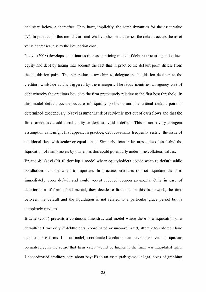
2.8 Results vs. Empirical data

In table 2.3, I summarize some results. Here, I highlight that the probability that the Senior

Bond is fully paid is 86.7%, while for the Junior Bond this probability is equal to 68.7%.

In the next subparagraph, I present details on cumulative DPs, recovery rate and yield spreads.

44

Liquidation Cost 1,83%Average V at the default 43,37%Yield to Maturity Senior 5,7%Yield to Maturity Junior 9,6%Yield Spread 3,6%Cumulative default pr at T 31,3%Cumulative default pr before T 24,38%Pr. Senior paid in full 86,68%

Pr. Junior paid in full 68,67%

Recovery Rate 52,80%

Tab. 2.3 – Some results

2.8.1 Cumulative DPS

In order to test my hypothesis, I calculate the cumulative default probabilities present

implicitly in the model and I compare these data with the cumulative DPs observed in

literature and computed empirically.

In particular, I use the average cumulative default frequencies for B-rated debt as function of

horizon, as given by Moody’s (2011) for the period 1983 – 2010 as my parameter of

comparison.

Figure 2.1 – Cumulative default probabilities

0

0,1

0,2

0,3

0,4

0,5

1 2 3 4 5 6 7 8 9 10

my DPs vs. empirical data

my DPs Empirical default probabilities

45

Matching my data with Moody’s data, it is evident that my DPs are very different from

empirical data. I believe that it depends on the fact that usually bonds are coupon bonds while

one of my main hypothesis (as in literature) is that bonds are ZCB.

In addition, I remind that I set my model on US market, while Moody’s data are global data.

In particular, it is important to point out that my d (grace period) is equal to 1 as in US, but I

don’t have any “global” reference.

2.8.2 Recovery Rate

My average Asset Value in case of default is equal to 43.4%, while the recovery rate (on

average) is 52.8%. This value is not very different from the value empirically found in

literature 51% - 52% (as above highlighted). I point out that this outcome is very close to

empirical data principally thanks to the presence of liquidation cost.

2.8.3 Yield Spread

I find that the yield to maturity for the senior bond is equal to 5.7%, while for the junior bond

this rate is equal to 9.6%. Therefore, the credit spread for junior bond (3.6%) is smaller than

the value that is empirically found in literature (4.7%).

This difference, again, is attributable to the fact that in this framework there are not coupon

bonds. Indeed, in chapter 3, with the introduction of coupons, I will get results more

satisfying.

46

2.8.4 Empirical cumulative DPs vs. old models

I show below a comparison between the DPs found in my model and these probabilities

computed using an adaptation of my model in which I assume that: the grace period is equal to

0.01; there aren’t Liquidation costs; and there is only one type of Zero Coupon Bond.

With these hypothesis, indeed, I obtain a particular case (hit and default models) that replicate

the “old” models present in literature.

Figure 2.2 – Cumulative default probabilities

0

0,1

0,2

0,3

0,4

0,5

1 2 3 4 5 6 7 8 9 10

my dps vs. old models

my DPs old models

0

0,1

0,2

0,3

0,4

0,5

0,6

1 2 3 4 5 6 7 8 9 10

old models vs. empirical data

Empirical default probabilities old models

Analyzing the figure 2.2, I could point out that my DPs are smaller than the probabilities

found with the “old models”. These results, furthermore, are very close to empirical DPs, even

if the last parallel is not practicable because the empirical data are computed for Coupon

Bonds and global data.

This fact become evident if I compare the recovery rate computed through the hit and default

models with those empirically found. Indeed, the recovery rate calculated empirically is equal

to 52%, while in the hit and default model this parameter is equal to 83%.

Even if I consider an hit and default model with LC and two types of Bond, I have the same

results. Indeed, I get: a recovery rate equal to 67%, that is very different from the empirical

47

value of 52%; and a yield spread equal to 3%, that is very far from the 4.70% reported by the

Lehman bond index.

The recovery rate is particularly high versus empirical data and this huge difference is

dependent on the fact that in these model a firm default as soon as the asset value hit the

barrier.

The credit spread is very different from the empirical data, because in these framework debts

are always zero coupon bonds.

It is evident, therefore, that hit and default models (old models) does not fit empirical data,

since the hypothesis of these models are not in line with the real world.

2.9 Hypothetical country

If I just change the level of the grace period from 1 to 0.65, I build an hypothetical case in

which the grace period is more or less equal to the average between US data and Swedish

data.

In this way, I try to point out that part of the difference between my results and empirical

results are dependent on the fact that I use the US reference as level of grace period.

Indeed, this change produce a moderate variation and, consequently, my cumulative default

probabilities become closer to empirical default probabilities (see figure 2.3).

I believe that the distance present between my results and empirical results is not equal to zero

because in this framework there are not coupons. Indeed, in Chapter 3 I will get results more

satisfying.

48

Figure 2.3 – Cumulative default probabilities

0

0,1

0,2

0,3

0,4

0,5

1 2 3 4 5 6 7 8 9 10

hypothetical country

my DPs Empirical default probabilities hyp. country

2.10 Sensitivity analysis

I now consider how my results are sensitive to the choices of my parameters. I start from the

base case, and then change various parameter choices in order to study the impact of these

parameters on the asset value, on recovery rate and on cumulative DPs.

2.10.1 Grace period (d)

In my base case the initial grace period is set equal to one year (as in Covitz, Han and Wilson,

2006), but it is shown by different authors that under different legal system the average time in

bankruptcy could be shorter or longer. Thoburn, for example, finds that in Sweden this period

is much shorter and equal to 2.5 months, while in 1990s in the US the time in bankruptcy was

longer than in the last years (18 – 24 months versus 12 months).

Therefore, I present a sensitivity analysis below in order to study the impact of the length of

the initial grace period on the price of the assets, the recovery rate and the default

probabilities.

49

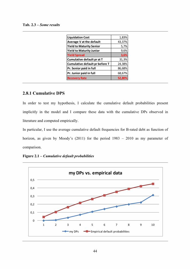
An increase of the grace period extends the time in bankruptcy and decreases the capacity of

the senior bondholders to extract value upon default (cfr. Figure 2.4).

Indeed, in this case decrease the probability that the senior bonds are fully paid. At the same

time, go down the cumulative default probabilities (it is more likely that the asset value

rebound up the threshold level), but the first effect prevail on the second effect.

Conversely, the Value of the Junior Bond and Equity price go up, due to the decrease of the

DPs (cfr. Figures 2.4 and 2.5).

Figure 2.4 – Sensitivity analysis: grace period (d)

17,5

18

18,5

19

19,5

20

0,5 0,75 1 1,25 1,5

Pric

e

Grace Period

Price Senior

12,6

12,8

13

13,2

13,4

13,6

0,5 0,75 1 1,25 1,5

Pric

e

Grace Period

Price Junior

As upon pointed out, when the grace period increases it is less likely the that the senior bonds

are fully paid. This means, as shown in Figures 2.5 and 2.6, that the Value of Asset (V) at time

of Default goes down and consequently the liquidation costs and recovery rate decrease

(remind that the LCs are a percentage of V and that recovery rate is equal to (1-

LC)*V(at_default)/F)).

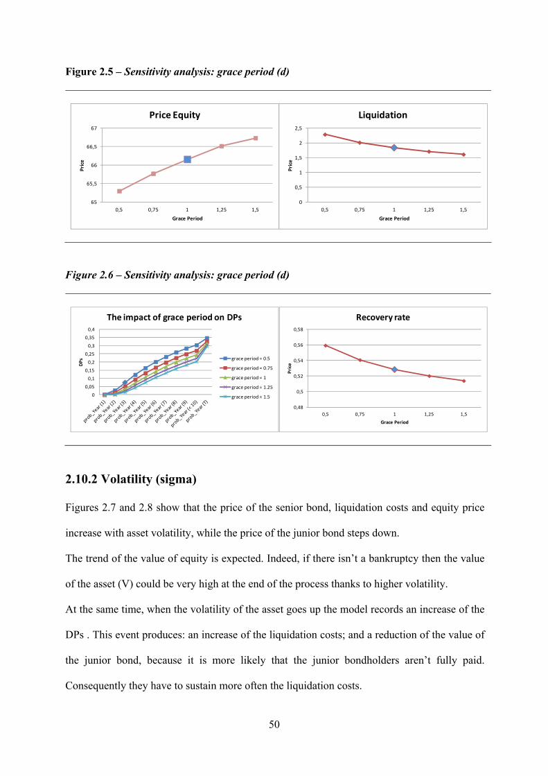
50

Figure 2.5 – Sensitivity analysis: grace period (d)

65

65,5

66

66,5

67

0,5 0,75 1 1,25 1,5

Pric

e

Grace Period

Price Equity

0

0,5

1

1,5

2

2,5

0,5 0,75 1 1,25 1,5

Pric

e

Grace Period

Liquidation

Figure 2.6 – Sensitivity analysis: grace period (d)

0,48

0,5

0,52

0,54

0,56

0,58

0,5 0,75 1 1,25 1,5

Pric

e

Grace Period

Recovery rate

0

0,05

0,1

0,15

0,2

0,25

0,3

0,35

0,4

DPs

The impact of grace period on DPs

grace period = 0.5

grace period = 0.75

grace period = 1

grace period = 1.25

grace period = 1.5

2.10.2 Volatility (sigma)

Figures 2.7 and 2.8 show that the price of the senior bond, liquidation costs and equity price

increase with asset volatility, while the price of the junior bond steps down.

The trend of the value of equity is expected. Indeed, if there isn’t a bankruptcy then the value

of the asset (V) could be very high at the end of the process thanks to higher volatility.

At the same time, when the volatility of the asset goes up the model records an increase of the

DPs . This event produces: an increase of the liquidation costs; and a reduction of the value of

the junior bond, because it is more likely that the junior bondholders aren’t fully paid.

Consequently they have to sustain more often the liquidation costs.

51

Whereas the value of the senior bond, as above reported, steps up until the volatility is so high

that the probability that the senior bondholders are fully paid decrease largely (because of the

liquidation costs trend and DPs’ variations).

Figure 2.7 – Sensitivity analysis: volatility

17,5

18

18,5

19

19,5

0,2 0,23 0,26 0,29 0,32 0,35 0,38

pric

e

sigma

Senior

8

10

12

14

16

18

0,2 0,23 0,26 0,29 0,32 0,35 0,38

pric

e

sigma

Junior

Figure 2.8 – Sensitivity analysis: volatility

64

65,5

67

68,5

70

0,2 0,23 0,26 0,29 0,32 0,35 0,38

pric

e

sigma

Equity

0

2

4

0,2 0,23 0,26 0,29 0,32 0,35 0,38

pric

e

sigma

Liquidation

The trend of the recovery rate, finally, depends on the evolution of the liquidation costs and of

the DPs (cfr. Figures 2.9).

52

Figure 2.9 – Sensitivity analysis: volatility

0

0,1

0,2

0,3

0,4

0,5

0,6

DPs

The impact of sigma on DPs

sigma = 0.20

sigma = 0.23

sigma = 0.26

sigma = 0.29

sigma = 0.32

sigma = 0.35

sigma = 0.38

0,25

0,375

0,5

0,625

0,75

0,2 0,23 0,26 0,29 0,32 0,35 0,38

pric

e

sigma

Recovery rate

2.10.3 The percentage of Senior Bond on the Total Debt

It is straightforward (and clear from figure 2.10) that the value of the two different type of

Bonds depends on gamma (parameter that measure the percentage of the senior bond on the

total debt) and that the Equity value does not change varying this parameter.

Also the Liquidation costs and DPs are constant (in this framework). Indeed, one of the main

hypothesis of the model is that the threshold level depends only on the Total Debt.

It is interesting, however, to show how change the probability that the senior bond is fully

paid (cfr. figure 2.11) varying gamma. When gamma is equal to 0.3 (30% of the total debt is

Senior), this probability is very close to 1, while when gamma is equal to 0.7 this value is

smaller than 0.75.

Conversely, the probability that the junior bond is fully paid is independent from the value of

gamma, because it depends on the DPs (that are constant).

53

Figure 2.10 – Sensitivity analysis: The percentage of Senior Bond on the Total Debt

0

5

10

15

20

25

30

0,3 0,4 0,5 0,6 0,7

pric

e

gamma

Senior

0

5

10

15

20

25

0,3 0,4 0,5 0,6 0,7

pric

e

gamma

Junior

Figure 2.11 – Sensitivity analysis: The percentage of Senior Bond on the Total Debt

0,5

0,75

1

0,3 0,4 0,5 0,6 0,7

prob

.

gamma

Prob. Senior fully paid

0,5

0,75

1

0,3 0,4 0,5 0,6 0,7

prob

gamma

Prob. Junior fully paid

2.10.4 Dividend yield (delta)

When a firm pays more dividend, the dynamic of the asset value (Brownian process) is more

stable (V increases more slowly). It is more likely that the company fails and, therefore, the

equity price decreases (cfr. Figure 2.13).

At the same time, the value of the junior bond steps down (figure 2.12), while the value of

Senior Bond is more or less constant. It depends on the fact that the new process produces a

decrease (very large) of the probability that junior bondholders is fully paid. Therefore, it is

more probable that the junior bondholders have to sustain the liquidation costs (and then these

costs step up).

54

Figure 2.12 – Sensitivity analysis: dividend yield

18

18,5

19

19,5

20

0 0,01 0,02 0,03 0,04

pric

e

delta

Senior

10

10,5

11

11,5

12

12,5

13

13,5

14

0 0,01 0,02 0,03 0,04

pric

e

delta

Junior

Figure 2.13 – Sensitivity analysis: dividend yield

30

35

40

45

50

55

60

65

70

0 0,01 0,02 0,03 0,04

pric

e

delta

Equity

1,5

2

2,5

3

0 0,01 0,02 0,03 0,04

pric

e

delta

Liquidation

From figure 2.14 it is clear that Recovery Rate, finally, is stable because the growth of the

liquidation costs and DPs are offset by the fact that the process is less variable (more often

junior pays for the bankruptcy / default happens in junior’s area).

55

Figure 2.14 – Sensitivity analysis: dividend yield

0,50 0,01 0,02 0,03 0,04

pric

e

delta

Recovery Rate

0,00%

5,00%

10,00%

15,00%

20,00%

25,00%

30,00%

35,00%

40,00%

45,00%

50,00%

DPs

The impact of delta on DPs

d = 0

d = 0.01

d = 0.02

d = 0.03

d = 0.04

2.10.5 Liquidation Costs

According to my base case, when there is liquidation, the bondholders (junior bondholders or

senior bondholders depend on the situation) have to sustain the liquidation cost equal to 20%.

I show the impact of a different level of liquidation cost on the bond prices in Figure 2.15

However, there is no impact on the equity price. In case of liquidation: 1) equityholders do not

receive anything; 2) they do not have to pay anything due to limited liability.

The larger price variation hits principally the junior debt price when the liquidation cost

increases gradually from 0% to 20%.

Conversely, if the liquidation cost goes up from 20%, the impact is heavier on the price of the

senior debt. Indeed, when the liquidation cost becomes bigger and bigger, it is most likely

that:

Vt - LC ≤ SD and consequently the senior debtholders have to sustain these costs.

56

Figure 2.15 – Sensitivity analysis: liquidation cost

18

18,5

19

19,5

0 0,1 0,2 0,3

pric

e

LC

Senior

11,5

12

12,5

13

13,5

14

14,5

15

0 0,1 0,2 0,3

pric

e

LC

Junior

It is straightforward that Recovery Rate decrease when the Liquidation costs increase (cfr.

Figure 2.16). Indeed, by construction the Recovery Rate is equal to ((1-LC)*V(at_default)/F)

and here there are not variation of the DPs.

Figure 2.16 – Sensitivity analysis: liquidation cost

0

0,5

1

1,5

2

2,5

3

0 0,1 0,2 0,3

pric

e

LC

Liquidation

0

0,5

1

0 0,1 0,2 0,3

LC

Recovery Rate

2.10.6 Leverage Ratio

Figure 2.17 provides the evolution of bond values for different level of financial leverage

ratio. Due to the rise of the Total Debt, there is an increase on the value of the senior and

junior bonds. In reality, the price of the junior bond goes up until the effect of the total debt’s

growth is greater than the effect of the increase of the Liquidation costs and of the DPs.

57

Figure 2.17 – Sensitivity analysis: leverage ratio

13

16

19

22

25

28

31

34

0,55 0,657 0,75 0,85 0,95 1

pric

e

LR

Senior

10

11

12

13

14

15

0,55 0,657 0,75 0,85 0,95 1

pric

e

LR

Junior

In line with my expectation, equity goes down (cfr. Figure 2.18), considered that the

shareholders are the residual claimants. Liquidation costs step up, due to the fact that these

costs are function of: 1) Liquidation Value; 2) Threshold level; 3) Total Debt (F).

Figure 2.18 – Sensitivity analysis: leverage ratio

45

50

55

60

65

70

75

0,55 0,657 0,75 0,85 0,95 1

pric

e

LR

Equity

0

2,5

5

7,5

0,55 0,657 0,75 0,85 0,95 1

pric

e

LR

Liquidation

When LR rises then the threshold level is higher and, therefore, it is more likely that Vt could

below the barrier. This implies that cumulative default probabilities increase with LR (cfr.

Figure 2.19).

58

Figure 2.19 – Sensitivity analysis: leverage ratio

0,4

0,45

0,5

0,55

0,6

0,55 0,657 0,75 0,85 0,95 1

pric

e

LR

Recovery Rate

0

0,1

0,2

0,3

0,4

0,5

0,6

DPs

The impact of LR on DPs

LR = 0.55

LR = 0.6571

LR = 0.75

LR = 0.85

LR = 1

2.10.7 Threshold's parameter (Omega)

The following figures (2.20 and 2.21) show that the Price of the Senior Bond and the

Liquidation Costs go up when there is a positive variation of omega (Threshold's parameter).

This results are in with the expectation because when omega increases the barrier is higher.

Figure 2.20 – Sensitivity analysis: Threshold's parameter

16,25

17,5

18,75

20

21,25

0,7 0,75 0,8 0,85 0,9 0,95 1

pric

e

omega

Senior

10

11,25

12,5

13,75

15

0,7 0,75 0,8 0,85 0,9 0,95 1

pric

e

omega

Junior

It is interesting to highlight from figure 2.20 that the price of the Junior Bond decreases when

omega passes from 0.7 to 0.9 and then increase. It depends on the fact that the liquidation

costs’ rise offset the effect related to the barrier’s variation.

59

Cumulative DPs (cfr. Figure 2.22) step up when the threshold barrier is higher and,

consequently, equity decreases because the equity holders are residual claimants (cfr. Figure

2.21)

The recovery rate increases (cfr. Figure 2.22), but the variation is modest because of the

liquidation costs’ trend. In practice, the evolution of LC offset the benefits linked to an higher

barrier.

Figure 2.21 – Sensitivity analysis: Threshold's parameter

60

62,5

65

67,5

70

0,7 0,75 0,8 0,85 0,9 0,95 1

pric

e

omega

Equity

0

2,5

5

0,7 0,75 0,8 0,85 0,9 0,95 1

pric

e

omega

Liquidation

Figure 2.22 – Sensitivity analysis: Threshold's parameter

0

0,125

0,25

0,375

0,5

0,625

0,75

0,875

1

0,7 0,75 0,8 0,85 0,9 0,95 1

pric

e

omega

Recovery Rate

0

0,05

0,1

0,15

0,2

0,25

0,3

0,35

0,4

DPs

The impact of omega on DPs

omega = 0.7

omega = 0.75

omega = 0.8

omega = 0.85

omega = 0.9

omega = 0.95

omega = 1

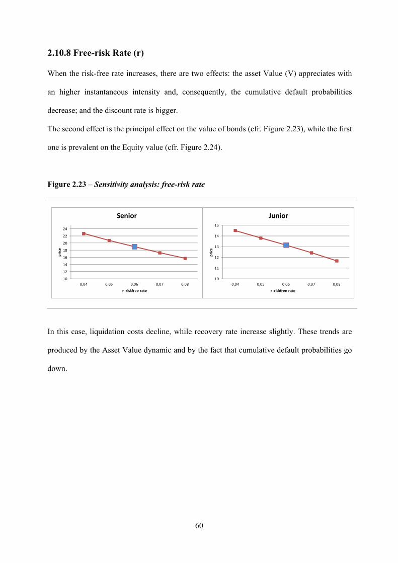
60

2.10.8 Free-risk Rate (r)

When the risk-free rate increases, there are two effects: the asset Value (V) appreciates with

an higher instantaneous intensity and, consequently, the cumulative default probabilities

decrease; and the discount rate is bigger.

The second effect is the principal effect on the value of bonds (cfr. Figure 2.23), while the first

one is prevalent on the Equity value (cfr. Figure 2.24).

Figure 2.23 – Sensitivity analysis: free-risk rate

10

12

14

16

18

20

22

24

0,04 0,05 0,06 0,07 0,08

pric

e

r ‐riskfree rate

Senior

10

11

12

13

14

15

0,04 0,05 0,06 0,07 0,08

pric

e

r ‐riskfree rate

Junior

In this case, liquidation costs decline, while recovery rate increase slightly. These trends are

produced by the Asset Value dynamic and by the fact that cumulative default probabilities go

down.

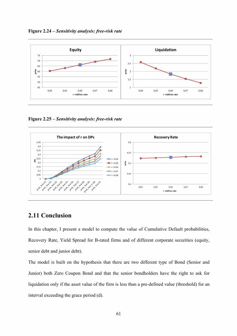
61

Figure 2.24 – Sensitivity analysis: free-risk rate

45

50

55

60

65

70

75

0,04 0,05 0,06 0,07 0,08

pric

e

r ‐riskfree rate

Equity

1

1,5

2

2,5

3

0,04 0,05 0,06 0,07 0,08

pric

e

r ‐riskfree rate

Liquidation

Figure 2.25 – Sensitivity analysis: free-risk rate

0,4

0,45

0,5

0,55

0,6

0,04 0,05 0,06 0,07 0,08

pric

e

r ‐riskfree rate

Recovery Rate

0

0,05

0,1

0,15

0,2

0,25

0,3

0,35

0,4

0,45

DPs

The impact of r on DPs

r = 0.04

r = 0.05

r = 0.06

r = 0.07

r = 0.08

2.11 Conclusion

In this chapter, I present a model to compute the value of Cumulative Default probabilities,

Recovery Rate, Yield Spread for B-rated firms and of different corporate securities (equity,

senior debt and junior debt).

The model is built on the hypothesis that there are two different type of Bond (Senior and

Junior) both Zero Coupon Bond and that the senior bondholders have the right to ask for

liquidation only if the asset value of the firm is less than a pre-defined value (threshold) for an

interval exceeding the grace period (d).

62

These assumptions make my model more realistic than the hit and default models, in which

there is just one type of debt , there isn’t liquidation cost and the grace period is equal to one

day (d = 0.01).

The first result is that my “internal” cumulative DPs are different from empirical data

(Moody’s) and it depends principally on the fact that bonds, in reality, are coupon bonds while

one of my main hypothesis (as in literature) is that bonds are ZCB. Indeed, when in Chapter 3

I add coupons to my model, I get results very satisfying and very close to empirical data.

Another element that influence this results is that I set my model on US market, while

Moody’s data are global data. It is important to point out that my d (grace period) is equal to 1

as in US, but we don’t have any “global” reference for this parameter.

I remind, anyway, that if change the value of the grace period from 1 to 0.65 my results get

closer to empirical data.

The recovery rate, computed through my framework, is 52.8% (on average). This value,

however, is very close to the value empirically found in literature 51% - 52%, while my credit

spread for junior bond (3.6%) is smaller than the value that is empirically found in literature

(4.7%).

It is important, anyway, to point out that all results of the sensitivity analysis are in line with

expectations and with the results historically found in literature.

At the same time, I verify the reliability of the hit and default models (old models), matching

the same variables (cumulative DPs and recovery rate) with the empirical data. I get that

cumulative Dps are very close to empirical DPs, but the recovery rate is equal to 83% while

the empirically data is 52%.

This difference is dependent on the fact that the empirical data are computed for Coupon

Bonds and are relative to global data.

63

Even if I consider an hit and default models with LC and two types of Bond, I have the same

results. In fact, I get a recovery rate equal to 67%, that is very different from the empirical

value of 52% and a yield spread equal to 3%, that is very far from the 4.7% reported by the

Lehman bond index.

The results of this type of model are, therefore, not very satisfying. Indeed, these models fit

relatively well cumulative default probabilities, but they are not able to find value of recovery

rate and of yield spreads in line with those empirically found.

I conclude, therefore, that: 1) my model works theoretically and it is more realistic than old

models, but the results are not comparable with the empirical data; 2) hit and default models

(old models) present some problems, even if cumulative DPs are in line with empirical data.

64

CHAPTER 3 – A Real Option Model with a Junior Coupon Bond

3 Brief Introduction

In Chapter 2, I built a real option model different from classic structural models because I

consider a grace period, two type of bonds and liquidation cost. Whit this new approach I

wanted to fit some empirical data and in particular the trend of cumulative default

probabilities, the value of the recovery rate and the value of the yield spreads.

The results were mixed since I was not able to replicate the evolution of cumulative default

probabilities for B-rated firm.

Therefore, in this Chapter I introduce another hypothesis that is innovative respect to the

classical real option model. In practice, I assume that one of the two bonds (the junior bond) is

a coupon bond.

The outcomes are very satisfying, since I get cumulative default probabilities, a recovery rate

and a yield spread very close to empirical data.

I could assert that: in my construction the presence of two type of bond and of liquidation cost

have a positive impact on the value of recovery rate and yield spreads; and the presence of

grace period and the introduction of coupons are crucial ingredients for fitting empirical data.

Instead, if I adapt the old models, considering two type of bonds and liquidation cost, I get

results very different from empirical data and this difference does not change if I also

introduce coupons in this framework.

65

3.1 Structural Model

In order to make my model more realistic, I change one of the structural model’s main

hypothesis. In this framework, indeed, I assume that one of two bond is a Coupons Bond. In

particular, I suppose that the Junior Bond is a Coupons Bond, while the Senior Bond is still a

Zero Coupon Bond.

This setting could replicate a real situation in which a firm has bank debt guaranteed and

rolling (sort of ZCB) and another debt (Bond) with coupons issued on Financial Market.

The Coupon C is determined such that a time 0, Junior Debt is priced at par:

PJB = (1 – γ) * F (3.1)

Others assumptions are consistent with/to those introduced in Chapter 2. Here, I show again

these hypothesis for simplicity:

- the default event allows the creditor (Senior Bondholders) to force immediate liquidation

through its safety covenants;

- liquidation is declared when the asset value of the firm falls below distress threshold for a

period that goes beyond the pre-determined grace time (denoted by d).

- shareholders have a residual claim on the cash flows generated by the firm’s assets unless

the value of these assets reaches the default threshold and remains below that threshold for the

grace period.

- assets are continuously traded in an arbitrage-free and complete market with riskless

borrowing or lending at a constant rate r.

66

3.1.1 Model assumptions

3.1.1.1 Asset Value

I assume again that the firm asset value evolves according to a diffusion process. This process

has constant volatility, does not depend on the capital structure but, in this case, presents a

jump because of the coupon payment. In practice, every time there is a coupons’ payment the

value of Asset VT jump down and the dynamic restart from (VT – C).

The process is always a risk neutral process and all parameters (rt, δt, σv) are assumed constant

trough time.

3.1.1.2 Debt

The firm has a total debt F, of which part is senior debt (SD) and the remaining part is junior

debt (JD):

SD = γ*F (3.2)

JD = (1- γ)*F (3.3)

where γ is a parameter that measure the percentage of senior debt on total debt

The maturity of the Debt is equal to T and I consider here the case where the Senior Debt is

ZCB, while the Junior Debt is Coupon Debt.

3.1.1.3 Liquidation Costs

Liquidation costs are still a fraction of asset value Vt at the moment of the default and are

equal to:

67

LC = ρ*Vt (3.4)

where ρ is a parameter that measure liquidation cost

3.1.1.4 The threshold level

My default boundary depends only upon the principal value of debt and it is not affected by

my parameters and by coupon payments. Therefore, the threshold level K, which is time

independent, is equal to:

K = ω F (3.5)

where 0≤ω ≤1 and this parameter set the level of threshold

In practice, the threshold level is constant between t and T and there aren’t jumps because of

the presence of the coupons.

3.1.1.5 Random Variables

In order to determine the value of corporate securities, I define the same random variables

introduced in Chapter 2:

gtk = sup s≤t | Vs = Ks (3.6)

θkt = inf t≥0 | t- gt

k ≥ d, Vt ≤ Kt (3.7)

68

where gtk is the last time before t that the value of the firm’s assets crossed the threshold value

K, and θkt is the liquidation time, i.e., the first time the value of the firm’s assets spent d units

of time consecutively below the default threshold.

3.2 The valuation of corporate securities

In this paragraph, I present the new pay-off of firm’s stakeholders. In particular, it is clear that

the presence of coupons impact on the condition/constrain of my equation.

It is necessary, however, to point out that in this framework when there is liquidation, junior

bondholders receive the present value of coupons (Σ Couponst) that include the accrued

interest.

3.2.1 Equity Value

In case of liquidation Equity holders, as residual claimants, do not receive anything. If there is

not liquidation (if VT > F + last coupon), at debt maturity T, Equity holders receive the

maximum between zero and the difference between the firm’s asset value VT and the face

value of the total debt (F). The Equity holders pay-off, therefore, is represented by this

equation:

S(VT , T , gtk) = max (VT - F, 0)*1θ

k> t = (3.8)

At any time before the debt maturity, if bankruptcy has not occurred, the value of Equity

holders claim is given by:

St (Vt , T , gtk) = e-r(T-t) EQ

t [max (VT - F, 0)*1θk

> t] (3.9)

VT – F if VT > F + Coupon and θk > T 0 otherwise

69

3.2.2 Senior Debt

The value of the senior debt (SD) is equal to:

1) face value if the firm is not prematurely liquidated, and the asset value of the firm VT is

greater than the face value of Debt plus the last coupon;

2) face value if the firm is not prematurely liquidated, and the asset value of the firm VT is

smaller than the face value of Debt plus last coupon but greater than the face value of Debt

plus liquidation cost;

3) VT – LC if the firm is not prematurely liquidated, and VT is smaller than the face value of

SD plus liquidation cost;

4) face value if the firm is prematurely liquidated, and Vt is greater than the face value of SD

plus liquidation cost;

5) Vt – LC if the firm is liquidated, and Vt is less than the face value of SD plus liquidation

cost.

In summary, I define the possible values of SD, to be:

SDt (Vt , T , gtK) = (3.10)

The expression (3.10) may be rewritten as:

SDt (Vt,T,gtK) = EQ

t[SD*e-r(T-t)*1θk

>T*1VT≥F]+EQt [SD*e-r(T-t)*1θ

k>T*1VT<F+c*1VT≥ SD+LC

+EQt[(VT - LC)*e-r(T-t)*1θ

k>T*1VT<F+coup*1VT < SD+LC]+Eq

t [SD*e-r(θk -t)*1θk≤ T*1Vt ≥ SD+LC ]

+EQt [(Vt – LC)*e-r(θk -t)*1θ

k≤ T*1Vt < SD+LC ] (3.11)

SD if VT ≥ F + coupon and θk > T SD if VT < F + coupon, VT ≥ SD + LC and θk > T VT - LC if VT < F + coupon, VT < SD + LC and θk > T SD if Vt ≥ SD + LC and θk ≤ T Vt - LC if Vt < SD + LC and θk ≤ T

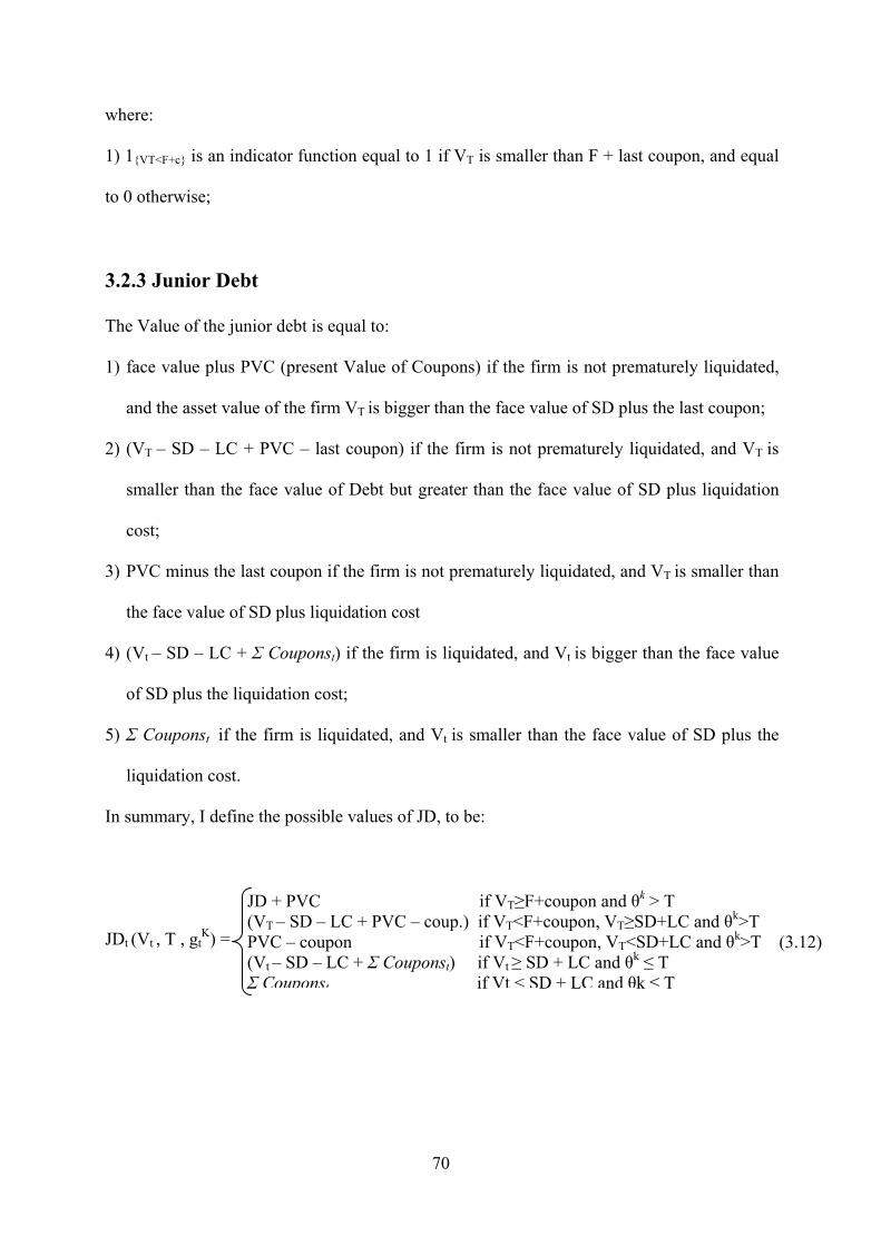
70

where:

1) 1VT<F+c is an indicator function equal to 1 if VT is smaller than F + last coupon, and equal

to 0 otherwise;

3.2.3 Junior Debt

The Value of the junior debt is equal to:

1) face value plus PVC (present Value of Coupons) if the firm is not prematurely liquidated,

and the asset value of the firm VT is bigger than the face value of SD plus the last coupon;

2) (VT – SD – LC + PVC – last coupon) if the firm is not prematurely liquidated, and VT is

smaller than the face value of Debt but greater than the face value of SD plus liquidation

cost;

3) PVC minus the last coupon if the firm is not prematurely liquidated, and VT is smaller than

the face value of SD plus liquidation cost

4) (Vt – SD – LC + Σ Couponst) if the firm is liquidated, and Vt is bigger than the face value

of SD plus the liquidation cost;

5) Σ Couponst if the firm is liquidated, and Vt is smaller than the face value of SD plus the

liquidation cost.

In summary, I define the possible values of JD, to be:

JDt (Vt , T , gtK) =

JD + PVC if VT≥F+coupon and θk > T (VT – SD – LC + PVC – coup.) if VT<F+coupon, VT≥SD+LC and θk>T PVC – coupon if VT<F+coupon, VT<SD+LC and θk>T (3.12) (Vt – SD – LC + Σ Couponst) if Vt ≥ SD + LC and θk ≤ T Σ Couponst

if Vt < SD + LC and θk ≤ T

71

The expression (3.12) may be rewritten as:

JDt(Vt,T,gtK) = EQ

t[((JD)*e-r(T-t)+PVC)*1θk> T*1VT≥ F+c+EQ

t[(((VT–SD–LC–coupon)*e-r(T-t))

+ PVC)*1θk> T*1VT< F+c*1VT ≥ SD+LC]+EQ

t[((coupon)*e-r(T-t)+PVC)1θk≤ T*1VT< F+c*1VT<

SD+LC]+EQt[(Vt – SD – LC + Σ Couponst)*e-r(θk-t)*1θ

k≤ T *1Vt ≥ SD+LC]+EQ

t[(Σ Couponst)*e-

r(θk-t)*1θk≤ T *1Vt < SD+LC (3.13)

where:

1) 1VT≥F+c is an indicator function equal to 1 if VT is smaller than F + last coupon, and equal

to 0 otherwise;

In table 3.1, I report the payoffs given to the different stakeholders.

Tab. 3.1 – Payoffs

PAYOFFS TOVT ≥ F + Coupon and θk > T

VT < F + Coupon, VT ≥ SD+LC and θk > T

VT < F + Coupon, VT < SD+LC and θk > T

F ≥ Vt ≥ SD+LC and θk ≤ T Vt < SD+LC and θk ≤ T

EQUITYHOLDERS VT – F 0 0 0 0SENIOR BONDHOLDERS SD SD VT - LC SD Vt - LCJUNIOR BONDHOLDERS JD + PVC (VT – SD – LC + PVC - couponT) PVC - couponT (Vt – SD – LC + Σ Couponst) Σ Couponst

TOTAL VT + PVC (VT - LC) + (PVC -couponT) (VT - LC) + (PVC -couponT) Vt - LC + Σ Couponst Vt - LC + Σ Couponst

Liquidation before TBond repayment or Liquidation at the end (T)

3.3 Benchmark

Also, in this case, I am able to compute: default probabilities over the time interval (0,T]; the

implied recovery rate RR = (1-LC)*Vl / F; the yield to maturity and the yield spread of the two

different obligations. I use this value in order to test the consistency of my model.

The outcomes, as pointed out below, are very satisfying. Indeed, I get a recovery rate and a

yield spread in line with those empirically found and a trend of cumulative default

72

probabilities very similar to empirical cumulative DPs with a perfect coincidence at the end of

the process (at T = 10 years).

In addition, my results are better than those found using an adaption of old models (hit and

default models).

3.4 Numerical implementation

I use, again, a Monte-Carlo simulation approach that considers 150,000 sample paths for

calculating bond prices, equity value, cumulative default probabilities, and recovery rate. The

solution found are stable up to the second digit.

3.5 Parameters’ choice

I assume that firm’s capital structure is constituted by ordinary stock, senior debt and junior

debt. Both the obligations have a maturity of 10 years. Junior Debt is a Coupon Bond, while

Senior Debt is a Zero Coupon Bond.

I utilize the same real value used in Chapter 2 for the parameters present in the Model. The

two main differences are: the Coupon C is determined such that a time 0, Junior Debt is priced

at par; and every time there is a coupons’ payment the value of Asset VT jump down and the

dynamic restart from (VT – C).

In tables 3.2, I summarize the parameters choice:

73

Tab. 3.2 – Parameters

Parameter Symbol Value AssumedTime to Maturity T 10Pre‐defined grace period d 1Percentage of SD on Total Debt γ 0,5Default free interest rate r 0,06Volatility of the asset of the firm σ 0,29Liquidation Cost LC 0,2Threshold's parameter ω 0,85Dividend yield δ 0

Initial Value of Assets V0 100

Leverage Ratio LR 0,657Debt Face Value F 65,7Debt Coupon rate i 0,1078dt=0.01; dt 0,01paths 150.000

3.6 Results

Some results are reported in table 3.3, while considerations about cumulative DPs, recovery

rate and yield spreads are presented in the next sections.

However, I point out, here, that the probability that the Senior Bond is fully paid is 76.9%,

while for the Junior Bond this probability is equal to 53.28%. Also, in this framework, the

Junior Bondholders pay more often the liquidation cost.

Tab. 3.3 – Some results

Liquidation Cost 2,65%Average V at the default 41,95%Yield Senior 5,49%Yield Junior 11,07%Cumulative default pr at T 46,72%Cumulative default pr before T 38,13%Pr. Senior paid in full 76,90%Pr. Junior paid in full 53,28%

Recovery Rate 51,08%

74

3.6.1 Cumulative DPS

In order to test my hypothesis, I calculate the cumulative default probabilities present

implicitly in the model and I compare these data with the cumulative DPs observed in

literature (Moody’s 2011).

Matching my data with Moody’s data, it is evident that my DPs are really close to empirical

data and that at the end (at T =10 years) these probabilities are coincident.

The introduction of coupons is a crucial assumption. Indeed, my results have an impressive

improvement when I introduce this hypothesis.

The light difference depends on the fact that I set my model on US market, while Moody’s

data are global data. In particular, it is important to point out that my d (grace period) is equal

to 1 as in US, but we don’t have any “global” reference.

Figure 3.1 – Cumulative default probabilities

0

0,1

0,2

0,3

0,4

0,5

1 2 3 4 5 6 7 8 9 10

Coupons case vs Empirical data

base case Empirical default probabilities

75

3.6.2 Recovery Rate

The average Asset Value in case of default is equal to 41.95%, while the recovery rate (on

average) is 51.05%. This value is in line with the value empirically found in literature 51% -

52% (as above highlighted).

The presence of coupon and the consequent growth of DPs produce a reduction of my

recovery rate versus those found in chapter 2.

3.6.3 Yield Spread

I find that the yield to maturity for the senior bond is equal to 5.49%, while for the junior bond

this rate is equal to 11.07%.

Therefore, the credit spread for junior bond (5.07%) is very close to the value that is

empirically found in literature (4.7%).

In practice, the values (for recovery rate and yield spreads) that I found implicitly from my

model are equal to the values found in a couple of empirical research (Huang and Huang,

2003 and Altman and Kishore, 2006 etc.) and I get this value without any type of calibration.

3.6.4 Empirical cumulative DPs vs. old models

I show below a graph where:

- The blue line represents my results;

- The violet line represents the DPs computed through an adaption of my model in which I

assume that the grace period is equal to 0.01 (such as in old models) and that there aren’t

Liquidation costs;

- The red line represents empirical data.

76

Figure 3.2 – Cumulative default probabilities

00,05

0,10,15

0,20,25

0,30,35

0,40,45

0,50,55

0,6

prob_Year (1) prob_Year (2) prob_Year (3) prob_Year (4) prob_Year (5) prob_Year (6) prob_Year (7) prob_Year (8) prob_Year (9) prob_Year (10)

my DPs, Empirical data and old models

my DPs Empirical default probabilities hit&default

Analyzing this figure, I could point out that the adaption of old models (g = 0.01 with two

type of bonds, of which one Junior with coupons) give back results very different from

Moody’s data.

In practice, if I consider an adaption of old models with two type of debt and coupons, I get

results very far from empirical data. This means that the presence of grace period represent the

crucial assumption that allow me to match empirical data.

This fact is confirmed if I compare the recovery rate and yield spread computed through the

hit and default model with those empirically found. Indeed, the recovery rate calculated

empirically is equal to 52%, while in the hit and default model this parameter is equal to

83.8%; and the yield spread equal to 3.6% is far from the 4.70% reported by the Lehman bond

index.

Even if I consider an hit and default models (old models) with LC, I have the same results. In

fact, I get a recovery rate equal to 67.5%, that is still very different from the empirical value of

52%.

77

I could, therefore, assert that old models are not able to represent real world. Indeed, I showed

in chapter 2 that without coupons these models do not fit recovery rate and yield spreads and,

in addition, I highlight in this chapter that, if I include coupons, the main results do not change

and on the contrary cumulative DPs become very different from empirical data.

3.7 Hypothetical country

Here, I present a variation of my model, in which I change just one variable and the coupon

rate. In practice, in this particular setting I consider a grace period g = 0.65 (versus 1.0 in the

base case) and, in addition, I vary the coupon rate in order to satisfy the hypothesis that the

junior debt is priced at par.

Again, I choose the new level of the grace period equal to (more or less) the average between

US data (1 year) and Swedish data (2.5 months).

The outcomes are very satisfying due that new results match really well the empirical data.

This confirm that the difference between my data and empirical data is due mainly to the fact

that my model is built on US data while empirical data (cumulative default probabilities) are

global.

Indeed, it is important to remind that I don’t have the global value for grace period, but I know

that is equal to 1 in US.

I explain the light difference present at the end of the period between my data and real data

such as a difference dependent on the fact that in my model it in not possible to renew the debt

at the expiration date, while in the real world it is very likely to roll over the debt.

78

Figure 3.3 – Cumulative default probabilities

3.8 Sensitivity analysis

I now consider how my results are sensitive to the choices of my parameters. I start from the

base case, and then change various parameter choices in order to study the impact of these

parameters on the asset value, recovery rate and cumulative DPs.

3.8.1 Grace period (g)

Here, I present a sensitivity analysis in order to study the impact of the length of the initial

grace period on the price of the assets, the recovery rate and the default probabilities.

I remind that an increase of the grace period extends the time in bankruptcy and decreases the

capacity of the senior bondholders to extract value upon default (cfr. Figure 3.4).

Indeed, in this case: 1) the probability that the senior bonds are fully paid decrease; 2)

cumulative default probabilities go down (it is more likely that the asset value rebound up the

threshold level; 3) the first effect prevail on the second effect.

0,00

0,10

0,20

0,30

0,40

0,50

0,60

1 2 3 4 5 6 7 8 9 10

Hypothetical country

hyp. country Empirical default probabilities

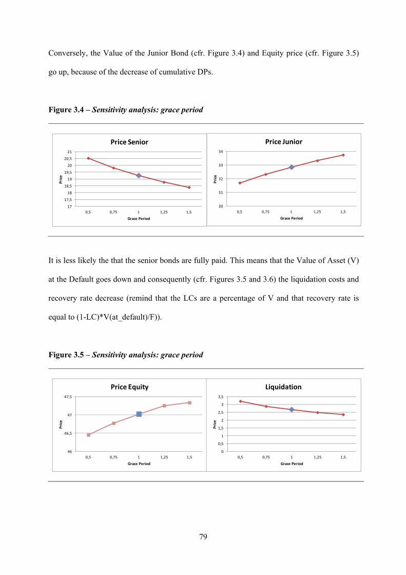
79

Conversely, the Value of the Junior Bond (cfr. Figure 3.4) and Equity price (cfr. Figure 3.5)

go up, because of the decrease of cumulative DPs.

Figure 3.4 – Sensitivity analysis: grace period

17

17,5

18

18,5

19

19,5

20

20,5

21

0,5 0,75 1 1,25 1,5

Pric

e

Grace Period

Price Senior

30

31

32

33

34

0,5 0,75 1 1,25 1,5Pr

ice

Grace Period

Price Junior

It is less likely the that the senior bonds are fully paid. This means that the Value of Asset (V)

at the Default goes down and consequently (cfr. Figures 3.5 and 3.6) the liquidation costs and

recovery rate decrease (remind that the LCs are a percentage of V and that recovery rate is

equal to (1-LC)*V(at_default)/F)).

Figure 3.5 – Sensitivity analysis: grace period

46

46,5

47

47,5

0,5 0,75 1 1,25 1,5

Pric

e

Grace Period

Price Equity

0

0,5

1

1,5

2

2,5

3

3,5

0,5 0,75 1 1,25 1,5

Pric

e

Grace Period

Liquidation

80

Figure 3.6 – Sensitivity analysis: grace period

0,44

0,46

0,48

0,5

0,52

0,54

0,56

0,5 0,75 1 1,25 1,5

Pric

e

Grace Period

Recovery rate

0

0,1

0,2

0,3

0,4

0,5

0,6

DPs

The impact of grace period on DPs

grace period = 0.5

grace period = 0.75

grace period = 1

grace period = 1.25

grace period = 1.5

3.8.2 Volatility (sigma)

From Figure 3.8 it is evident that liquidation costs and equity price increase when asset

volatility goes up, while from Figure 3.7 it is clear that the price of the junior bond steps

down.

The trend of the value of equity is expected. Indeed, if there is not a bankruptcy then the value

of the asset (V) could be very high at the end of the process.

At the same time, when the volatility of the asset goes up the model records an increase of the

DPs. This event produces an increase of liquidation costs and a reduction of the value of the

junior bond. It is more likely that the junior bondholders are not fully paid and consequently

they have to sustain more often the liquidation costs.

Whereas the value of the senior bond (cfr. Figure 3.7) steps up until the volatility is equal to

0.29. From that point, the probability that the senior bondholders are paid in full decrease

largely and consequently the value of this type of debt starts to decrease.

81

Figure 3.7 – Sensitivity analysis: volatility

18,5

19

19,5

0,2 0,23 0,26 0,29 0,32 0,35 0,38

pric

e

sigma

Senior

28

30

32

34

36

38

40

0,2 0,23 0,26 0,29 0,32 0,35 0,38

pric

e

sigma

Junior

Figure 3.8 – Sensitivity analysis: volatility

40

42

44

46

48

50

52

54

56

0,2 0,23 0,26 0,29 0,32 0,35 0,38

pric

e

sigma

Equity

0

2

4

0,2 0,23 0,26 0,29 0,32 0,35 0,38

pric

e

sigma

Liquidation

The trend of the recovery rate, finally, depends on the evolution of: 1) liquidation costs; 2)

cumulative DPs.

82

Figure 3.9 – Sensitivity analysis: volatility

0

0,1

0,2

0,3

0,4

0,5

0,6

DPs

The impact of sigma on DPs

sigma = 0.20

sigma = 0.23

sigma = 0.26

sigma = 0.29

sigma = 0.32

sigma = 0.35

sigma = 0.38

0,25

0,5

0,75

0,2 0,23 0,26 0,29 0,32 0,35 0,38

pric

e

sigma

Recovery rate

3.8.3 The percentage of Senior Bond on the Total Debt

It is straightforward that the value of the two different type of Bond depends on the percentage

gamma of senior bond on the total debt.

Equity value goes up when the value of gamma increase (cfr. Figure 3.11). This pattern is

dependent on the fact that the equityholders as residual claimants benefit from the reduction of

coupons payment. Because of this reduction, cumulative default probabilities4 and Liquidation

costs go down while recovery rate increase slowly (cfr. Figures 3.11 and 3.12).

Figure 3.10 – Sensitivity analysis: The percentage of Senior Bond on the Total Debt

0

5

10

15

20

25

30

0,3 0,4 0,5 0,6 0,7

pric

e

gamma

Senior

05

10152025303540455055

0,3 0,4 0,5 0,6 0,7

pric

e

gamma

Junior

4 In this framework when I change gamma, cumulative DPs are not constant as in Chapter 2.

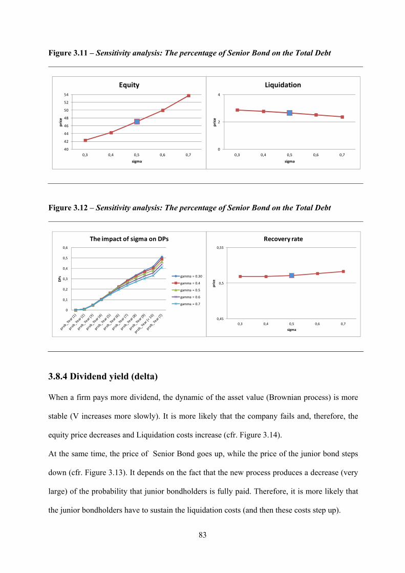
83

Figure 3.11 – Sensitivity analysis: The percentage of Senior Bond on the Total Debt

40

42

44

46

48

50

52

54

0,3 0,4 0,5 0,6 0,7

pric

e

sigma

Equity

0

2

4

0,3 0,4 0,5 0,6 0,7

pric

e

sigma

Liquidation

Figure 3.12 – Sensitivity analysis: The percentage of Senior Bond on the Total Debt

0

0,1

0,2

0,3

0,4

0,5

0,6

DPs

The impact of sigma on DPs

gamma = 0.30

gamma = 0.4

gamma = 0.5

gamma = 0.6

gamma = 0.7

0,45

0,5

0,55

0,3 0,4 0,5 0,6 0,7

pric

e

sigma

Recovery rate

3.8.4 Dividend yield (delta)

When a firm pays more dividend, the dynamic of the asset value (Brownian process) is more

stable (V increases more slowly). It is more likely that the company fails and, therefore, the

equity price decreases and Liquidation costs increase (cfr. Figure 3.14).

At the same time, the price of Senior Bond goes up, while the price of the junior bond steps

down (cfr. Figure 3.13). It depends on the fact that the new process produces a decrease (very

large) of the probability that junior bondholders is fully paid. Therefore, it is more likely that

the junior bondholders have to sustain the liquidation costs (and then these costs step up).

84

The evolution of the value of the senior bond derives from the trend of cumulative default

probabilities above specified and from the fact that the Value at the default that is constant

thanks to the stability of the process.

Figure 3.13 – Sensitivity analysis: dividend yield

18

19

20

0 0,01 0,02 0,03 0,04

pric

e

delta

Senior

20

22,5

25

27,5

30

32,5

35

0 0,01 0,02 0,03 0,04

pric

e

delta

Junior

Figure 3.14 – Sensitivity analysis: dividend yield

20

30

40

50

0 0,01 0,02 0,03 0,04

pric

e

delta

Equity

0

1

2

3

4

5

0 0,01 0,02 0,03 0,04

pric

e

delta

Liquidation

Recovery Rate is very stable, because the growth of the liquidation costs and DPs are offset by

the fact that the process is less variable (cfr. Figure 3.15).

85

Figure 3.15 – Sensitivity analysis: dividend yield

0

0,1

0,2

0,3

0,4

0,5

0,6

0,7

DPs

The impact of sigma on DPs

delta = 0

delta = 0.01

delta = 0.02

delta = 0.03

delta = 0.04

0

0,2

0,4

0,6

0,8

1

0 0,01 0,02 0,03 0,04

pric

e

delta

Recovery Rate

3.8.5 Liquidation Costs

When there is liquidation, junior bondholders or senior bondholders have to sustain the

liquidation cost. Therefore, the impact of variation in liquidation cost influence only the value

of these two assets.

Here, as in Chapter 2, indeed, there is no impact on the equity price. In case of liquidation the

equityholders don’t receive anything and, at the same time, they don’t have to pay anything

due to limited liability.

From Figure 3.16 it is clear that Junior debt price is more affected by the variation of

liquidation cost when this parameter increases gradually from 0% to 20%.

Conversely, if the liquidation cost goes up from 20% to 30%, the impact is heavier on the

price of the senior debt. Indeed, when the liquidation cost becomes bigger and bigger, it is

more likely that:

Vt - LC ≤ SD (the senior debtholders have to sustain these costs).

86

Figure 3.16 – Sensitivity analysis: liquidation cost

17,5

18

18,5

19

19,5

20

20,5

0 0,1 0,2 0,3

pric

e

LC

Senior

30,531

31,532

32,533

33,534

34,535

35,5

0 0,1 0,2 0,3

pric

e

LC

Junior

Recovery Rate, on the other hand, decrease when the Liquidation costs increase. Indeed,

Recovery Rate is equal to ((1-LC)*V(at_default)/F).

Finally, there are not variation of the cumulative Default Probabilities, because there is

liquidation when the firm is already on default.

Figure 3.17 – Sensitivity analysis: liquidation cost

0

0,5

1

1,5

2

2,5

3

3,5

4

4,5

0 0,1 0,2 0,3

pric

e

LC

Liquidation

0

0,5

1

0 0,1 0,2 0,3

LC

Recovery Rate

3.8.6 Leverage Ratio

When there is an increase of the value of the Total Debt, the price of the senior and junior

bonds rise proportionally (cfr. Figure 3.18).

87

Clearly, the price of the junior bond goes up until the effect of the total debt’s growth is offset

by the increase of the Liquidation costs and of the cumulative Default Probabilities.

Figure 3.18 – Sensitivity analysis: leverage ratio

13

16

19

22

25

28

31

34

0,55 0,657 0,75 0,85 1

pric

e

LR

Senior

28

30

32

34

36

0,55 0,657 0,75 0,85 1pr

ice

LR

Junior

I find, as expected, that the equity price goes down (cfr. Figure 3.19), while the cumulative

Default Probabilities increase (cfr. Figure 3.20). In fact, when a firm has more debt, it is easier

to have default.

Figure 3.19– Sensitivity analysis: leverage ratio

30

35

40

45

50

55

0,55 0,657 0,75 0,85 1

pric

e

LR

Equity

0

2,5

5

7,5

0,55 0,657 0,75 0,85 1

pric

e

LR

Liquidation

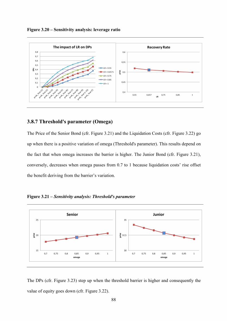
88

Figure 3.20 – Sensitivity analysis: leverage ratio

0,4

0,45

0,5

0,55

0,6

0,55 0,657 0,75 0,85 1

pric

e

LR

Recovery Rate

0

0,1

0,2

0,3

0,4

0,5

0,6

0,7

0,8

DPs

The impact of LR on DPs

LR = 0.55

LR = 0.6571

LR = 0.75

LR = 0.85

LR = 1

3.8.7 Threshold's parameter (Omega)

The Price of the Senior Bond (cfr. Figure 3.21) and the Liquidation Costs (cfr. Figure 3.22) go

up when there is a positive variation of omega (Threshold's parameter). This results depend on

the fact that when omega increases the barrier is higher. The Junior Bond (cfr. Figure 3.21),

conversely, decreases when omega passes from 0.7 to 1 because liquidation costs’ rise offset

the benefit deriving from the barrier’s variation.

Figure 3.21 – Sensitivity analysis: Threshold's parameter

15

20

25

0,7 0,75 0,8 0,85 0,9 0,95 1

pric

e

omega

Senior

30

32,5

35

0,7 0,75 0,8 0,85 0,9 0,95 1

pric

e

omega

Junior

The DPs (cfr. Figure 3.23) step up when the threshold barrier is higher and consequently the

value of equity goes down (cfr. Figure 3.22).

89

From Figure 3.23 it also clear that the recovery rate, on the other hand, increases but the

variation is modest because of the liquidation costs’ trend.

Figure 3.22 – Sensitivity analysis: Threshold's parameter

40

42,5

45

47,5

50

0,7 0,75 0,8 0,85 0,9 0,95 1

pric

e

omega

Equity

0

2

4

0,7 0,75 0,8 0,85 0,9 0,95 1pr

ice

omega

Liquidation

Figure 3.23 – Sensitivity analysis: Threshold's parameter

0

0,5

1

0,7 0,75 0,8 0,85 0,9 0,95 1

pric

e

omega

Recovery Rate

0

0,1

0,2

0,3

0,4

0,5

0,6

DPs

The impact of omega on DPs

omega = 0.7

omega = 0.75

omega = 0.8

omega = 0.85

omega = 0.9

omega = 0.95

omega = 1

3.8.8 Free-risk Rate (r)

When the risk-free rate increases, there are two effects: the asset Value (V) appreciates with

an higher instantaneous intensity and, consequently, the cumulative default probabilities

decrease; and the discount rate became bigger and bigger.

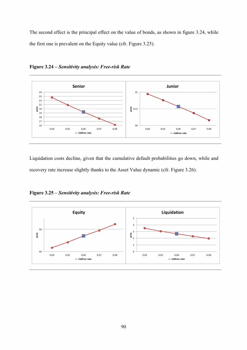
90

The second effect is the principal effect on the value of bonds, as shown in figure 3.24, while

the first one is prevalent on the Equity value (cfr. Figure 3.25).

Figure 3.24 – Sensitivity analysis: Free-risk Rate

16

17

18

19

20

21

22

23

24

0,04 0,05 0,06 0,07 0,08

pric

e

r ‐ riskfree rate

Senior

30

32,5

35

0,04 0,05 0,06 0,07 0,08pr

ice

r ‐ riskfree rate

Junior

Liquidation costs decline, given that the cumulative default probabilities go down, while and

recovery rate increase slightly thanks to the Asset Value dynamic (cfr. Figure 3.26).

Figure 3.25 – Sensitivity analysis: Free-risk Rate

40

50

0,04 0,05 0,06 0,07 0,08

pric

e

r ‐ riskfree rate

Equity

0

1

2

3

4

5

0,04 0,05 0,06 0,07 0,08

pric

e

r ‐ riskfree rate

Liquidation

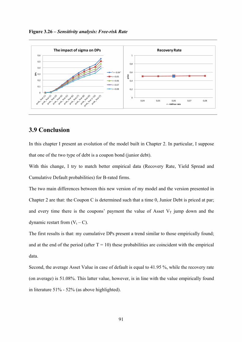
91

Figure 3.26 – Sensitivity analysis: Free-risk Rate

0

0,1

0,2

0,3

0,4

0,5

0,6

DPs

The impact of sigma on DPs

"r = 0.04"

r = 0.05

r = 0.06

r = 0.07

r = 0.08

0

0,2

0,4

0,6

0,8

1

0,04 0,05 0,06 0,07 0,08

pric

e

r ‐ riskfree rate

Recovery Rate

3.9 Conclusion

In this chapter I present an evolution of the model built in Chapter 2. In particular, I suppose

that one of the two type of debt is a coupon bond (junior debt).

With this change, I try to match better empirical data (Recovery Rate, Yield Spread and

Cumulative Default probabilities) for B-rated firms.

The two main differences between this new version of my model and the version presented in

Chapter 2 are that: the Coupon C is determined such that a time 0, Junior Debt is priced at par;

and every time there is the coupons’ payment the value of Asset VT jump down and the

dynamic restart from (Vt – C).

The first results is that: my cumulative DPs present a trend similar to those empirically found;

and at the end of the period (after T = 10) these probabilities are coincident with the empirical

data.

Second, the average Asset Value in case of default is equal to 41.95 %, while the recovery rate

(on average) is 51.08%. This latter value, however, is in line with the value empirically found

in literature 51% - 52% (as above highlighted).

92

Third, yield to maturity for the senior bond is equal to 5.49%, while for the junior bond this

rate is equal to 11.07%. Therefore, the credit spread for junior bond (5.07%) is in line with the

value that is empirically found in literature (4.7%).

Fourth, the probability that the Senior Bond is fully paid is 76.9%, while for the Junior Bond

this probability is equal to 53.28%.

The interesting thing, however, is that I capture these stylized fact with real ingredients . All

parameters’ value are chosen using data found in a couple of empirical papers.

In addition, when I change the value of the grace period from 1 to 0.65 (equal to the average

between the Us value and Swedish value) my DPS fit very well the empirical.

In this latter case (hypothetical country), I demonstrate that the difference between my data

and empirical data is due mainly to the fact that my model is built on US data while empirical

data (cumulative default probabilities) are global. Indeed, in my base case the key parameter d

(grace period) is set equal to 1 (that represent the US value), while empirical data are global

data and it is demonstrate that in a couple of Country it is possible to have a liquidation in less

than 1 year.

I could assert that my model with coupons match very well empirical data. In particular when

I consider the “hypothetical country”, varying the level of d (grace period).

It is important, then, to point out that I made a couple of sensitivity analysis and the results are

in line with expectations and with the results historically found in literature.

Finally, If I adapt old models to this framework, I get, again, that: cumulative Dps are very

different from empirical DPs; the recovery rate calculated empirically is equal to 52%, while

in the hit and default model this parameter is equal to 83.8%; the yield spread is equal to 3.6%

and it is very far from the 4.70% reported by the Lehman bond index.

This happens, even if I consider an hit and default model with LCs. Indeed, I get a recovery

rate equal to 67%, that is very different from the empirical value of 52%.

93

Therefore, I show again that old models are inefficient and not able to match empirical data.

On the contrary, I could affirm that, with my approach, I am able to reproduce really well the

real world and that it is crucial the combination of these two ingredients: the presence of the

grace period and of coupons.

94

Appendix A – A Real Option Model with a Senior Coupon Bond

A. Brief Introduction

Here, I present a different adaption of my model in which I assume that the Senior Bond is the

coupon bond. In this way, I want to show that the results found in chapter 3 do not depend on

the hypothesis that the Junior Bond is the coupon bond.

In other word, I try to demonstrate that it is fundamental the presence of coupons in the model

and it is not important which bond is the zero coupon bond and which one is the coupon bond.

The outcomes are in line with expectations and confirm that it is crucial the presence of

coupons. Indeed, I get a recovery rate and a yield spreads very close to empirical value and

my cumulative default probabilities follow the trend of data found empirically.

A.1 Structural Model

As pointed out above, I assume that the Senior Bond is a Coupon Bond, while the Junior Bond

is a Zero Coupon Bond. This setting could replicate a real situation in which a firm has a bank

debt with coupons or a plain vanilla bond, while junior debt is a debt versus stakeholders.

The Coupon C is determined such that a time 0, Senior Debt is priced at par:

PSB = (γ) * F (a.1)

A.2 The valuation of corporate securities

Here, I show the new pay-off of equityholders and of bondholders and I point out that, when

there is liquidation, senior bondholders receive the present value of coupons (Σ Couponst) and

this value include the accrued interest.

95

A.2.1 Equity Value

Also in this framework, in case of liquidation Equity holders, as residual claimants, do not

receive anything. Therefore, if there is not liquidation, at debt maturity T, Equity holders

receive the maximum between zero and the difference between the firm’s asset value VT and

the face value of the total debt (F). The Equity holders pay-off is represented by this equation:

S(VT , T , gtk) = max (VT - F, 0)*1θ

k> t = (a.2)

At any time before the debt maturity, if bankruptcy hasn’t occurred, the value of Equity

holders claim is given by:

St (Vt , T , gtk) = e-r(T-t) EQ

t [max (VT - F - coupon, 0)*1θk

> t] (a.3)

A.2.2 Senior Debt

The value of the senior debt (SD) is equal to:

- face value plus PVC (present Value of Coupons) if the firm is not prematurely liquidated,

and the asset value of the firm VT is greater than the face value of Debt plus the last

coupon;

- face value plus PVC (present Value of Coupons) if the firm is not prematurely liquidated,

and the asset value of the firm VT is greater than the face value of Debt plus liquidation cost

and last coupon;

- VT – LC + PVC – last coupon if the firm is not prematurely liquidated, and VT is smaller

than the face value of SD plus liquidation cost and last coupon;

- face value + Σ Couponst if the firm is liquidated, and Vt is greater than the face value of SD

plus liquidation cost;

VT – F if VT > F + Coupon and θk > T 0 otherwise

96

- Vt – LC + Σ Couponst if the firm is liquidated, and Vt is less than the face value of SD plus

liquidation cost.

In summary, I define the possible values of SD, to be:

SDt (Vt , T , gtK) =

The expression (a.4) may be rewritten as:

SDt (Vt,T,gtK) = EQ

t[(SD*e-r(T-t)+PVC)*1θk

>T*1VT≥F]+EQt[(SD*e-r(T-t)+PVC)*1θ

k>T*

*1VT<F+c*1VT≥SD+LC+c+EQt[((VT-LC-c)*e-r(T-t))+PVC)*1θ

k>T*1VT<F+c*1VT<SD+LC]+Eq

t[(SD

+ Σ Coupt)*e-r(θk -t)*1θk≤ T*1Vt ≥ SD+LC] +EQ

t [(Vt – LC + Σ Coupt )*e-r(θk -t)*1θk≤ T*1Vt <

SD+LC] (a.5)

where:

1) 1VT ≥ SD + LC + c. is an indicator function equal to 1 if VT is greater than SD + LC + last

coupon, and equal to 0 otherwise;

2) 1VT < SD + LC + c. is an indicator function equal to 1 if VT is smaller than SD + LC, and equal

to 0 otherwise.

A.2.3 Junior Debt

The Value of the junior debt is equal to:

- face value if the firm is not prematurely liquidated, and the asset value of the firm VT is

bigger than the face value of TD plus the last coupon;

SD + PVC if VT ≥ F + coupon and θk > T SD + PVC if VT < F + coupon, VT ≥ SD + LC + coupon and θk > T VT–LC+PVC– coup. if VT < F + coupon, VT < SD + LC + coupon and θk > T SD + Σ Coupt if Vt ≥ SD + LC and θk ≤ T Vt – LC + Σ Coupt if Vt < SD + LC and θk ≤ T (a.4)

97

- (VT – SD – LC – coupon) if the firm is not prematurely liquidated, and VT is smaller than

the face value of Debt but greater than the face value of SD plus liquidation cost and last

coupon;

- 0 if the firm is not prematurely liquidated, and VT is smaller than the face value of SD plus

liquidation cost and last coupon;

- (Vt – SD – LC) if the firm is liquidated, and Vt is bigger than the face value of SD plus the

liquidation cost and accrued interest;

- 0 if the firm is liquidated, and Vt is smaller than the face value of SD plus the liquidation

cost and accrued interest.

In summary, I define the possible values of JD, to be:

JDt (Vt , T , gtK) =

The expression (a.6) may be rewritten as:

JDt(Vt,T,gtK) = EQ

t[((JD)*e-r(T-t))*1θk> T*1VT≥ F + c+EQ

t[((VT–SD–LC–coupon)*e-r(T-

t))*1θk>T*1VT<F+coupon*1VT ≥ SD + LC + c]+EQ

t[(Vt – SD – LC)*e-r(θk-t)*1θk≤ T*1Vt ≥ SD + LC]

(a.7)

In table a.1, I point out the payoffs given to the different stakeholders and computed

analytically above from (a.3) to (a.7).

JD if VT≥F+coupon and θk > T (VT – SD – LC – coupon) if VT<F+coupon, VT≥SD+LC+coupon and θk>T 0 if VT<F+coupon, VT<SD+LC+coupon and θk>T (Vt – SD – LC) if Vt ≥ SD + LC + a.c. and θk ≤ T 0 if Vt < SD + LC + a.c. and θk ≤ T (a.6)

98

Tab. a.1 – Payoffs

PAYOFFS TOVT ≥ F + Coupon and θk > T

VT < F + Coupon, VT ≥ SD+LC+coupon and θk > T

VT < F + Coupon, VT < SD+LC+coupon and θk > T

F ≥ Vt ≥ SD+LC+a.i. and θk

≤ TVt < SD+LC+a.i. and θk ≤ T

EQUITYHOLDERS VT – F 0 0 0 0SENIOR BONDHOLDERS SD + PVC SD + PVC VT – LC + PVC - couponT SD + Σ Coupt +a.i. Vt – LC + Σ Coupt

JUNIOR BONDHOLDERS JD (VT – SD – LC – couponT) 0 (Vt – SD – LC) 0

TOTAL VT + PVC (VT - LC) + (PVC -couponT) (VT - LC) + (PVC -couponT) Vt - LC + Σ Couponst + a.i. Vt - LC + Σ Couponst + a.i.

Bond repayment or Liquidation at the end (T) Liquidation before T

A.3 Benchmark

I use, again, default probabilities over the time interval (0,T], the implied recovery rate RR =

(1-LC)*Vl / F and the yield spread as parameter in order to test the consistency of my model.

A.4 Numerical implementation

I use, also in this case, a Monte-Carlo simulation approach that considers 150,000 sample

paths for calculating bond prices, equity value, cumulative default probabilities, and recovery

rate and the solution are stable up to the second digit.

A.5 Parameters’ choice

I assume that firm’s capital structure is constituted by ordinary stock, senior debt and junior

debt. Both the obligations have a maturity of 10 years. Junior Debt is a Zero Coupon Bond,

while Senior Debt is a Coupon Bond.

I utilize the same real value used in Chapter 2 for the parameters present in the Model. The

two main differences are: the Coupon C is determined such that a time 0, Senior Debt is

priced at par; and every time there is the coupons’ payment the value of Asset VT jump down

and the dynamic restart from (VT – C).

Table a.2 report the parameters’choice.

99

Tab. a.2 – Parameters

simulazioni zcb

Parameter Symbol Value AssumedTime to Maturity T 10Pre‐defined grace period d 1Percentage of SD on Total Debt γ 0,5Default free interest rate r 0,06Volatility of the asset of the firm σ 0,29Liquidation Cost LC 0,2Threshold's parameter ω 0,85Dividend yield δ 0

Initial Value of Assets V0 100

Leverage Ratio LR 0,657Debt Face Value F 65,7Debt Coupon rate i 0,06475dt=0.01; dt 0,01paths 150.000

A.6 Results

From table a.3 it is clear that the probability that the Senior Bond is fully paid is 79.28%,

while for the Junior Bond this probability is equal to 58.87%.

More details about default probabilities, recovery rate and yield spreads are pointed out from

paragraph a.6.1 to paragraph a.6.4.

Tab. a.3 – Some results

Liquidation Cost 2,36%Average V at the default 42,37%Yield Senior 6,58%Yield Junior 11,13%Cumulative default pr at T 41,13%Cumulative default pr before T 33,14%Pr. Senior paid in full 79,28%Pr. Junior paid in full 58,87%

Recovery Rate 51,59%

100

A.6.1 Cumulative DPS

Again, I test my model, matching my cumulative default probabilities with the cumulative

DPs observed in literature (Moody’s, 2011).

From this comparison, it is evident that my DPs are not very far from empirical data and that

at T = 10 these probabilities are very close. The light difference still depends on the fact that I

set my model on US market, while Moody’s data are global data. In particular, it is important

to point out that my d (grace period) is equal to 1 as in US, but we don’t have any “global”

reference.

Figure a.1 – Cumulative default probabilities

0

0,1

0,2

0,3

0,4

0,5

1 2 3 4 5 6 7 8 9 10

my DPs with coupons vs Empirical data

my DPs Empirical default probabilities

A.6.2 Recovery Rate

The average Asset Value in case of default is equal to 42.4%, while the recovery rate (on

average) is 51.59%. This value is in line with the value empirically found in literature 51% -

52% (as above highlighted).

101

A.6.3 Yield Spread

I find that the yield to maturity for the senior bond is equal to 6.58%, while for the junior bond

this rate is equal to 11.13%. Therefore, the credit spread for junior bond (5.13%) is not very

far / is in line with the value that is empirically found in literature (4.7%).

A.6.4 Empirical cumulative DPs vs. old models

I show below a graph where:

- The blue line represents my DPs;

- The violet line represents the DPs computed through an adaption of my model in which I

assume that the grace period is equal to 0.01 (such as in old models), there aren’t

Liquidation costs;

- The red line represents empirical data.

Figure a.2 – Cumulative default probabilities

00,05

0,10,15

0,20,25

0,30,35

0,40,45

0,50,55

0,6

prob_Year (1) prob_Year (2) prob_Year (3) prob_Year (4) prob_Year (5) prob_Year (6) prob_Year (7) prob_Year (8) prob_Year (9) prob_Year (10)

My DPs with coupons, Empirical data and hit and default model

my DPs Empirical default probabilities old models

102

Analyzing the figure, I could point out that the adaption of old models (g = 0.01 with two type

of debt, of which one Junior with coupons) give back results very different from Moody’s

data.

This latter fact is confirmed if I compare the recovery rate and yield spread computed through

the hit and default model with those empirically found. Indeed, the recovery rate calculated

empirically is equal to 52%, while in the hit and default model this parameter is equal to

83.7%; the yield spread is equal to 0.4% and it is very far from the 4.70% reported by the

Lehman bond index.

Even if I consider an hit and default models with LC, I have the same results. Indeed, I get a

recovery rate equal to 67%, that is very different from the empirical value of 52%;

Also in this case, I could affirm that old models are not able to outline the real world.

A.7 Hypothetical country

Also in this appendix, I present an hypothetical case, in which I change only one variable of

my model and the coupon rate in order to satisfy the hypothesis that the senior debt is priced

at par. In practice, I consider a grace period g = 0.65 (versus 1.0 in the base case), that is more

or less in line with the average between the grace period found for US and the grace period

found for Sweden.

The outcomes are very satisfying and they match empirical data very well.

These results, once again, confirm that the difference between my data and empirical data is

due mainly to the fact that my model is built on US data and for that I use a grace period equal

to 1, while empirical data (cumulative default probabilities) are global.

103

Figure a.3 – Cumulative default probabilities

0

0,1

0,2

0,3

0,4

0,5

1 2 3 4 5 6 7 8 9 10

hypothetical country

hyp. country Empirical default probabilities

A.8 Sensitivity analysis

I now consider how my results are sensitive to the choices of my parameters. I start from the

base case, and then change various parameter choices in order to study the impact of these

parameters on the asset value, on recovery rate and on the DPs.

The results are in line with the expectations and with the sensitivity analysis reported in

Chapter 2 and Chapter 3.

104

A.8.1 Grace period (d)

Figure a.4 – Sensitivity analysis: grace period

32,2

32,4

32,6

32,8

33

33,2

33,4

0,5 0,75 1 1,25 1,5

Pric

e

Grace Period

Price Senior

11

11,2

11,4

11,6

11,8

0,5 0,75 1 1,25 1,5

Pric

e

Grace Period

Price Junior

Figure a.5 – Sensitivity analysis: grace period

52

52,5

53

53,5

54

54,5

0,5 0,75 1 1,25 1,5

Pric

e

Grace Period

Price Equity

0

0,5

1

1,5

2

2,5

3

3,5

0,5 0,75 1 1,25 1,5

Pric

e

Grace Period

Liquidation

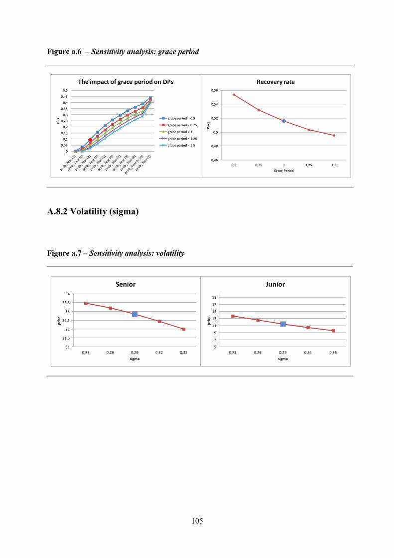
105

Figure a.6 – Sensitivity analysis: grace period

0,46

0,48

0,5

0,52

0,54

0,56

0,5 0,75 1 1,25 1,5

Pric

e

Grace Period

Recovery rate

0

0,05

0,1

0,15

0,2

0,25

0,3

0,35

0,4

0,45

0,5

DPs

The impact of grace period on DPs

grace period = 0.5

grace period = 0.75

grace period = 1

grace period = 1.25

grace period = 1.5

A.8.2 Volatility (sigma)

Figure a.7 – Sensitivity analysis: volatility

31

31,5

32

32,5

33

33,5

34

0,23 0,26 0,29 0,32 0,35

pric

e

sigma

Senior

5

7

9

11

13

15

17

19

0,23 0,26 0,29 0,32 0,35

pric

e

sigma

Junior

106

Figure a.8 – Sensitivity analysis: volatility

50

52

54

56

58

60

0,23 0,26 0,29 0,32 0,35

pric

e

sigma

Equity

0

2

4

0,23 0,26 0,29 0,32 0,35

pric

e

sigma

Liquidation

Figure a.9 – Sensitivity analysis: volatility

0

0,1

0,2

0,3

0,4

0,5

0,6

DPs

The impact of sigma on DPs

sigma = 0.23

sigma = 0.26

sigma = 0.29

sigma = 0.32

sigma = 0.35

0,25

0,5

0,75

0,23 0,26 0,29 0,32 0,35

pric

e

sigma

Recovery rate

107

A.8.3 The percentage of Senior Bond on the Total Debt

Figure a.10 – Sensitivity analysis: The percentage of Senior Bond on the Total Debt

05

101520253035404550

0,3 0,4 0,5 0,6 0,7

pric

e

gamma

Senior

0

5

10

15

20

25

0,3 0,4 0,5 0,6 0,7

pric

e

gamma

Junior

Figure a.11 – Sensitivity analysis: The percentage of Senior Bond on the Total Debt

4042444648505254565860

0,3 0,4 0,5 0,6 0,7

pric

e

sigma

Equity

0

2

4

0,3 0,4 0,5 0,6 0,7

pric

e

sigma

Liquidation

108

Figure a.12 – Sensitivity analysis: The percentage of Senior Bond on the Total Debt

0

0,05

0,1

0,15

0,2

0,25

0,3

0,35

0,4

0,45

0,5

DPs

The impact of sigma on DPs

gamma = 0.30

gamma = 0.4

gamma = 0.5

gamma = 0.6

gamma = 0.7

0,25

0,5

0,75

0,3 0,4 0,5 0,6 0,7

pric

e

sigma

Recovery rate

A.8.4 Dividend yield (delta)

Figure a.13 – Sensitivity analysis: dividend yield

30

31

32

33

34

35

0 0,01 0,02 0,03 0,04

pric

e

delta

Senior

0

2,5

5

7,5

10

12,5

15

0 0,01 0,02 0,03 0,04

pric

e

delta

Junior

109

Figure a.14 - Sensitivity analysis: dividend yield

20

30

40

50

60

0 0,01 0,02 0,03 0,04

pric

e

delta

Equity

0

1

2

3

4

5

0 0,01 0,02 0,03 0,04

pric

e

delta

Liquidation

Figure a.15 – Sensitivity analysis: dividend yield

0

0,1

0,2

0,3

0,4

0,5

0,6

0,7

DPs

The impact of sigma on DPs

delta = 0

delta = 0.01

delta = 0.02

delta = 0.03

delta = 0.04

0

0,2

0,4

0,6

0,8

1

0 0,01 0,02 0,03 0,04

pric

e

delta

Recovery Rate

110

A.8.5 Liquidation Costs

Figure a.16 – Sensitivity analysis: liquidation cost

31,5

32

32,5

33

33,5

34

0 0,1 0,2 0,3

pric

e

LC

Senior

10

10,5

11

11,5

12

12,5

13

13,5

0 0,1 0,2 0,3

pric

e

LC

Junior

Figure a.17 – Sensitivity analysis: liquidation cost

0

0,5

1

1,5

2

2,5

3

3,5

4

0 0,1 0,2 0,3

pric

e

LC

Liquidation

0

0,5

1

0 0,1 0,2 0,3

LC

Recovery Rate

111

A.8.6 Leverage Ratio

Figure a.18 – Sensitivity analysis: leverage ratio

25

28

31

34

37

40

43

46

49

0,55 0,657 0,75 0,85 0,95

pric

e

LR

Senior

10

12

0,55 0,657 0,75 0,85 0,95

pric

e

LR

Junior

Figure a.19 – Sensitivity analysis: leverage ratio

30

35

40

45

50

55

60

65

0,55 0,657 0,75 0,85 0,95

pric

e

LR

Equity

0,4

0,45

0,5

0,55

0,6

0,55 0,657 0,75 0,85 0,95

pric

e

LR

Recovery Rate

112

Figure a.20 – Sensitivity analysis: leverage ratio

0

2,5

5

7,5

0,55 0,657 0,75 0,85 0,95

pric

e

LR

Liquidation

0

0,1

0,2

0,3

0,4

0,5

0,6

0,7

DPs

The impact of LR on DPs

LR = 0.55

LR = 0.6571

LR = 0.75

LR = 0.85

LR = 0.95

A.8.7 Threshold's parameter (Omega)

Figure a.21 – Sensitivity analysis: Threshold's parameter

30

35

0,7 0,75 0,8 0,85 0,9 0,95 1

pric

e

omega

Senior

10

12,5

0,7 0,75 0,8 0,85 0,9 0,95 1

pric

e

omega

Junior

113

Figure a.22 – Sensitivity analysis: Threshold's parameter

50

52,5

55

57,5

60

0,7 0,75 0,8 0,85 0,9 0,95 1

pric

e

omega

Equity

0

2

4

0,7 0,75 0,8 0,85 0,9 0,95 1

pric

e

omega

Liquidation

Figure a.23 – Sensitivity analysis: Threshold's parameter

0

0,5

1

0,7 0,75 0,8 0,85 0,9 0,95 1

pric

e

omega

Recovery Rate

0

0,05

0,1

0,15

0,2

0,25

0,3

0,35

0,4

0,45

0,5

DPs

The impact of omega on DPs

omega = 0.7

omega = 0.75

omega = 0.8

omega = 0.85

omega = 0.9

omega = 0.95

omega = 1

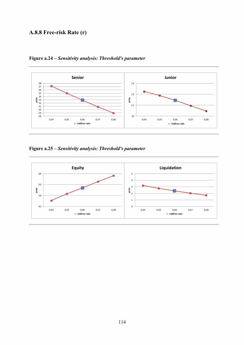
114

A.8.8 Free-risk Rate (r)

Figure a.24 – Sensitivity analysis: Threshold's parameter

2829303132333435363738

0,04 0,05 0,06 0,07 0,08

pric

e

r ‐ riskfree rate

Senior

10

11

12

13

0,04 0,05 0,06 0,07 0,08

pric

e

r ‐ riskfree rate

Junior

Figure a.25 – Sensitivity analysis: Threshold's parameter

45

50

55

60

0,04 0,05 0,06 0,07 0,08

pric

e

r ‐ riskfree rate

Equity

0

1

2

3

4

5

0,04 0,05 0,06 0,07 0,08

pric

e

r ‐ riskfree rate

Liquidation

115

Figure a.26 – Sensitivity analysis: Threshold's parameter

0

0,1

0,2

0,3

0,4

0,5

0,6

DPs

The impact of sigma on DPs

r = 0.04

r = 0.05

r = 0.06

r = 0.07

r = 0.08

0

0,2

0,4

0,6

0,8

1

0,04 0,05 0,06 0,07 0,08

pric

e

r ‐ riskfree rate

Recovery Rate

A.9 Conclusion

The results of this Appendix are in line with the results of Chapter 3. Therefore, I am sure that

the reliability (or capacity of matching cumulative default probabilities, recovery rate and

yield spread) of my model does not depend on the fact that the junior debt is a coupon bond.

As pointed out above, the combination of the presence of coupons and of the grace period

represents the crucial aspect of my model.

Therefore, I can assert that my framework fit really well empirical data because it is more

compliance with reality than old models.

116

References Acharya, V., & Carpenter, J. (2002). Corporate Bond Valuation and Hedging with Stochastic

Interest Rates and Endogenous Bankruptcy. Review of Financial Studies 15, 1355 - 1383.

Acharya, V., Huang, J., Subrahmanyam, M., & Sundaram, R. (2000). Costly Financing,

Optimal Payout Policies and the Valuation of Corporate Debt. Working Paper, New York

University.

Alderson, M., & Betker, B. (1995). Liquidation costs and capital structure. Journal of

Financial Economics 39, 45 - 69.

Altman, E., & Eberhart, A. (1994). Do priority provisions protect a bondholder's investment?

Journal of Portfolio Management 20, 67 - 75.

Altman, E., & Kishore, V. (1996). Almost everything you wanted to know about recoveries

on default bonds. Financial Analysts Journal, 57-64.

Anderson, R., & Sundaresan, S. (2000). A comparative study of structural models of

corporate bond yields: An exploratory investigation. Journal of Banking and Finance 24, 255

- 269.

Anderson, R., & Sundaresan, S. (1996). Design and valuation of debt contracts. Review of

Financial Studies, 37 - 68.

Anderson, R., Sundaresan, S., & Tychon, P. (1996). Strategic analysis of contingent claims.

European Economic Review 40, 871 - 881.

Andrade, G., & Kaplan, S. (1998). How Costly is (not Economic) Distress? Evidence from

Highly Leveraged Transactions that Became Distressed. Journal of Finance 53, 1443 - 1493.

Bakshi, G., Cao, C., & Chen, Z. (2000). Do call prices and the underlying stock always move

in the same direction? Review of Financial Studies 13, 549 - 584.

Bakshi, G., Cao, C., & Chen, Z. (1997). Empirical Performance of Alternative Option Pricing

Models. Journal of Finance 52 .

117

Bastes, D. (2003). Empirical option pricing: A retrospection. Journal of Econometrics, 387 -

404.

Bates, D. (1996). Jumps and stochastic volatility: exchange rate processes implicit in deutsche

mark Options. Review of Financial Studies 9 , 69 - 107.

Bates, D. (2000). Post-’87 Crash fears in the S&P 500 futures option market. Journal of

Econometrics 94, 181 - 238.

Bates, D. (1991). The crash of '87: Was it expected? The evidence from options markets.

Journal of Finance 46, 1009 - 1044.

Bebchuk, L. (2002). Ex Ante Costs of Violating Absolute Priority in Bankruptcy. The Journal

of Finance, 445 - 460.

Bebchuk, L., & Chang, H. (1992). Bargaining and the division of value in corporate

reorganization. Journal of Law, Economics and Organization 8, 253 - 279.

Betker, B. (1997). The administrative costs of debt restructurings: Some recent evidence.

Financial Management 26, 56 - 68.

Black, F., & Cox, J. (1976). Valuing corporate securities: Some effects of bond indenture

provisions. Juornal of Finance 31, 351 - 367.

Black, F., & Scholes, M. (1973). The pricing of options and corporate liabilities. Journal of

Political Economy 81, 637 - 654.

Bolton, P., & Scharfstein, D. S. (1996). Optimal Debt Structure and the Number of Creditors.

Journal of Political Economy 104, 1 - 25.

Brennan, M., & Schwartz, E. (1978). Corporate income taxes, valuation and the problem of

optimal capital structure. Journal of Business 51, 103 - 114.

Bris, A., & Welch, I. (2005). The Optimal Concentration of Creditors. Journal of Finance 60,

2193 - 2212.

118

Bris, A., Welch, I., & Zhu, N. (2006). The Costs of Bankruptcy: Chapter 7 Liquidation versus

Chapter 11 Reorganization. Journal of Finance 61, 1253 - 1303.

Broadie, M., & Glasserman, P. (1996). Estimating security price derivatives using simulation.

Management Science 42, 269 - 285.

Broadie, M., Chernov, M., & Sundaresan, S. (2007). Optimal Debt and Equity Values in the

Presence of Chapter 7 and Chapter 11. Journal of Finance .

Bruche, M. (2011). Creditor Coordination, Liquidation Timing, and Debt Valuation. Journal

of Financial and Quantitative Analysis 46, 1407 - 1436.

Bruche, M., & Naqvi, H. M. (2010). A structural model of debt pricing with creditor-

determined liquidation. Journal of Economic Dynamics and Control 34, 951 - 967.

Campbell, J., & Taksler, G. (2002). Equity Volatility and Corporate Bond Yields. Working

Paper, Harvard University .

Carr, P., & Wu, L. (2008). A Simple Robust Link between American Puts and Credit.

Working paper, Bloomberg and Baruch College.

Cathcart, L., & El-Jahel, L. (1998). Valuation of Defaultable Bonds. Journal of Fixed Income

8 , 65 - 78.

Chesney, M., Jeanblanc-Picque, M., & Yor, M. (1997). Brownian excursions and Parisian

barrier options. Advances in Applied Probabilities 29, 165 - 184.

Christensen, P., Flor, C., Lando, D., & Miltersen, K. (2000). Dynamic capital structure with

callable debt and debt renegotiations. Working Paper.

Collin-Dufresne, P., & Goldstein, R. (2001). Do credit spreads reflect stationary leverage

ratios? Journal of Finance 56, 1929 – 1957.

Collin-Dufresne, P., Goldstein, R., & Martin, J. (2001). The Determinants of Credit Spread

Changes. Journal of Finance 56, 2177 – 2207.

119

Cooper, I. A., & Davydenko, S. (2004). Using yield spreads to estimate expected returns on

debt and equity. working paper, London Business School.

Covitz, D., Han, M., & Wilson, S. (2006). Are Longer Bankruptcies really more costly?

Working Papaer Federal Reserve Board.

Cox, J., & Ross, S. (1976). The Valuation of Options for Alternative Sthocastic Processes.

Journal of Financial Economics 3, 145 - 166.

Cox, J., & RUBINSTEIN, M. (1985). Options Markets. Englewood Cliffs, NJ: Prentice-Hall.

D.Galai, Raviv, A., & Wiener, Z. (2007). Liquidation Triggers and the Valuation of Equity

and Debt. Working Paper, Hebrew University of Jerusalem.

Davydenko, S. (2007). When do firms default? A study of the default boundary. Working

paper, University of Toronto.

Delianedis, G., & Geske, R. (2001). The components of corporate credit spreads: Default,

recovery, tax, jumps, liquidity, and market factors. Working Paper Andersen School,

University of California.

Derman, E., & Kani, I. (1994). Riding on the Smile. Risk, 32 - 39.

Duffie, D., & Lando, D. (2001). Term structures of credit spreads with incomplete accounting

information. Econometrica 69, 633 - 664.

Duffie, D., & Singleton, K. (1997). An Econometric Model of the Term Structure of Interest-

Rate Swap Yields. The Journal of Finance 52, 1287 - 1321.

Duffie, D., Pan, J., & Singleton, K. (2000). Transform Analysis and asset pricing for affine

jump-diffusions. Econometrica 68, 1343 - 1376.

Dumas, B., Fleming, J., & Whaley, R. (1998). Implied volatility functions: empirical tests.

Journal of Finance 53, 2059 - 2106.

Dumitrescu, A. (2007). Ariadna, Valuation of defaultable bonds and debt restructuring.

Journal of Corporate Finance 13, 94 - 111.

120

Dupire, B. (1994). Pricing with a Smile. Risk, 18 - 20.

Elton, E. J., Gruber, M., Agrawal, D., & Mann, C. (2001). Explaining the Rate Spread on

Corporate Bonds. Journal of Finance 56 , 247 - 277.

Eom, Y., Helwege, J., & Huang, J. (2004). Structure models of bond pricing: an empirical

analysis. Review of Financial Studies, 499 - 544.

Ericsson, J., & Reneby, J. (2001). The valuation of corporate liabilities: Theory and Tests.

Working paper, McGill University and Stockholm School of Economics.

Fan, H., & Sundaresan, S. (2000). Debt valuation, renegotiation, and optimal dividend policy.

Review of financial studies 13, 1057 - 1099.

François, P., & Morellec, E. (2004). Capital Structure and Asset Prices: Some Effects of

Bankruptcy Procedures. The Journal of Business, 387 - 411.

Franks, J., & Sussman, O. (2005). Financial distress and bank restructuring of small to

medium size U.K. companies. The Review of Finance 9, 65–96.

Franks, J., & Torous, W. (1989). An empirical investigation of U.S. firms in reorganization .

Journal of Finance 5, 143 - 163.

Galai, D., & Masulis, R. (1976). The option pricing model and the risk factor of stock.

Journal of Financial Economics 3, 53 - 81.

Gesken, R. (1979). A Note on an Analytical Valuation Formula for Unprotected Americans

Options on Stocks with Known Dividends. Journal of Financial Economics 7, 375 - 380.

Gilson, S. C. (1997). Transactions costs and capital structure choice: Evidence from

financially distressed firms. Journal of Finance 52 , 161 - 196.

Gilson, S. C., John, K., & Lang, L. (1990). Troubled Debt Restructurings: An Empirical

Study of Private Reorganization of Firms in Default. Journal of Financial Economics 27, 315

- 353.

121

Goldstein, R., Ju, N., & Leland, H. (2001). An Ebit-based model od dynamic capital structure.

Journal of Business 74, 483 - 512.

Guha, R. (2002). Recovery of face value at default: Theory and empirical evidence. Working

paper, London Business School.

Haber, R., Schönbucher, P., & Wilmott, P. (1999). Pricing Parisan Options. Journal of

Derivatives, 71 - 79.

Harrison, J. M., & Pliska, S. (1981). Martingales and stochastic integrals in the theory of

continuous trading. Stochastic Processes and Their Applications 11, 215 - 260.

Haugen, R., & Senbet, L. (1978). The Insignificance of Bankruptcy Costs to the Theory of

Optimal Capital Structure . Journal of Finance 33, 383 - 393.

Hege, U., & Merra-Barral, P. (2000). Collateral, Renegotiation and the value of diffusely held

debt. Tilburg University.

Helwege, J. (1999). How long do junk bonds spend in default? Journal of Finance 54, 341 -

357.

Heston, S. (1993). A Closed-Form Solution of Options with Stochastic Volatility with

Applications to Bond and Currency Options. The Review of Financial Studies 6, 327 - 343.

Hotchkiss, E. (1995). Post-bankruptcy performance and management turnover. Journal of

Finance 50, 3 - 22.

Huang, J.-Z., & Huang, M. (2003). How much of corporate Treasure Yield Spread is due to

Credit Risk? Results from a New Calibration Approach. Working paper, Penn State

University.

Hugonnier, J. (1999). The Feynman-Kac Formula and Pricing Occupation Times Derivatives.

International Journal of Theoretical and Applied Finance 2, 153 - 178.

Hull, J., & White, A. (1987). The Pricing of Options with Stochastic Volatilities. Journal of

Finance 42, 281 - 300.

122

Hull, J., Nelken, I., & White, A. (2004). Mertons Model, Credit Risk and Volatility Skews.

Journal of Credit Risk 1, 8 - 23.

Warner, J.B. (1977). Bankruptcy costs: Some evidence. Journal of Finance 32, 337 - 347.

Jarrow, R., & Turnbull, S. (1995). Pricing derivatives on financial securities subject to credit

risk. Journal of Finance 50, 53 - 86.

Jarrow, R., Lando, D., & Turnbull, S. (1997). A Markov model for the term structure of credit

risk spreads. Review of Financial Studies 10, 481 - 523.

Jones, E., Mason, S., & Rosenfeld, E. (1984). Contingent claims analysis of corporate capital

structures: an empirical analysis. Journal of Finance 39, 611 - 625.

Kaiser, K. (1996). European bankruptcy laws: Implications for corporations facing financial

distress. Financial Management 25, 67 - 85.

Karatzas, I., & Shreve, S. (1991). Brownian motion and stochastic calculus. New York:

Springer Verlag.

Kealhofer, S., & Kurbat, M. (2001). The Default PredictionPower of The Merton Approach,

relative to Debt Ratings and Accounting Variables. Working paper, KMV Corp..

Leland, H. (1994). Corporate debt value, bond covenants, and optimal capital structure.

Journal of Finance 49, 1213–1252.

Leland, H. (2004). Predictions of default probabilities in strctural models of debt . Journal of

Investment Management 2, 5 - 20.

Leland, H., & Toft, K. (1996). Optimal capital structure, Endogenous bankruptcy, and the

Term structure of credit spreads. Journal of Finance 51, 987 - 1019.

Longstaff, F. (1990). The Valuation of options on yields. Journal of Financial Economics 26,

97 - 122.

Longstaff, F., & Schwartz, E. (1995). Valuing risky debt: A new approach. Journal of

Finance, 789 - 820.

123

Longstaff, F., Mithal, S., & Neis, E. (2005). Corporate yield spreads: Default risk or liquidity?

New evidence from the credit-default swap market. Journal of Finance 60, 2213 - 2253.

Maksimovic, V., & Phillips, G. (1998). Asset efficiency and reallocation decisions of

bankrupt firms. Journal of Finance 53, 1495 - 1532.

Mella-Barral, P. (1999). The dynamics of default and debt reorganization. Review of

Financial Studies.

Mella-Barral, P., & Perraudin, W. (1997). Strategic debt service. Journal of Finance 52, 531 -

556.

Mello, A., & Parsons, J. (1992). Measuring the agency cost of debt. Journal of Finance 47,

1887–1904.

Merton, R. (1974). On the pricing of corporate debt: The risk structure of interest rates.

Journal of Finance 29, 449 - 470.

Moody's. (2011). Corporate Default and Recovery Rates. Moody's investor service.

Moraux, F. (2004). Valuing corporate liabilities when the default threshold is not an

absorbing barrier. Working Paper, Université de Rennes.

Morellec, E. (2001). Asset liquidity, capital structure, and secured debt. Journal of Financial

Economics 61, 173 - 206.

Morse, D., & Shaw, W. (1988). Investing in bankrupt firms. Journal of Finance 43, 1193 -

1206.

Naik, V. ( 1993). Option Valuation and Hedging Strategies with Jumps in the Volatility of

Asset Returns. Journal of Finance 48, 1969 - 1984.

Naqvi, H. (2008). The Valuation of Corporate Debt with Default Risk. RMI Working Paper.

Paseka, A. (2003). Debt valuation with endogenous default and Chapter 11 reorganization.

Working Paper, University of Arizona.

124

Realdon, M. (2007). Valuation of the firm's liabilities when equity holders are also creditors.

Journal of Business Finance and Accounting 34 , 950 - 975.

Rubinstein, M. (1983). Displaced Diffusion Option Pricing. Journal of Finance 38, 213 - 217.

Schaefer, S., & Strebulaev, I. (2008). Structural models of credit risk are useful: Evidence

from hedge ratios on corporate bonds. Journal of Financial Economics, 1 - 19.

Schönbucher, P. (1998). Term Structure Modelling of Defaultable Bonds. Review of

Derivatives Research 2, 161 - 193.

Scott, L. (1987). Option Pricing when the Variance changes randomly: Theory, Estimation,

and an Application . Journal of Financial and Quantitative Analysis 22, 419 - 438.

Skiadopoulos, G. (2000). Volatility smile consistent option models: a survey. International

Journal of Theoretical and Applied Finance 4, 403 - 437.

Stein, E., & Stein, J. (1991). Stock Price Distributions with Stochastic Volatility: An Anaytic

Approach. Review of Financial Studies 4, 727 - 752.

Stohs, M., & Mauer, D. (1996). The determinants of corporate debt maturity structure.

Journal of Business 69, 279 - 312.

Tarashev, N. (2008). An empirical evaluation of structural credit risk models. International

Journal of Central Banking 41, 1 - 53.

Teixeria, J. (2007). An empirical analysis of structural models of corporate debt pricing.

Applied Financial Economics 17, 1141 - 1165.

Thorburn, K. (2000). Bankruptcy Auctions: Costs, debt recovery and firm survival. Journal of

Financial Economics 58, 337 - 368.

Titman, S. (1984). The Effect of Capital Structure on a Firm's Liquidation Decision . Journal

of Financial Economics 13, 137 - 151.

Uhrig-Homburg, M. (2002). Valuation of defaultable claims: A survey. Schmalenbach

Business Review 54, 24 - 57.

125

Varma, P., & Cantor, R. (2005). Determinants of Recovery Rates on Defaulted Bonds and

Loans for North American Corporate Issuers: 1983-2003. Journal of Fixed Income 14, 29 -

44.

Weiss, L., & Wruck, K. (1998). Information problems, conflicts of interest, and asset

stripping: Chapter 11’s failure in the case of Eastern Airlines. Journal of Financial Economics

48, 55 - 97.

White, M. (1996). The costs of corporate bankruptcy: A U.S.-European comparison. In

Corporate bankruptcy: Economic and legal perspectives. Cambridge University Press.

Wiggins, J. (1987). Option Values under Stochastic Volatilities. Journal of Financial

Economics 19, 351 - 372.

Wruck, K. (1990). Financial distress, reorganization, and organizational efficiency. Journal of

Financial Economics 27, 419 - 444.

Zhou, C. (2001). The Term Structure of Credit Spreads with Jump Risk. Journal of Banking

and Finance 25, 2015 – 2040.