Coupling between lumped and distributed models for blood flow problems

Comput Visual Sci 4: 111–124 (2001) Computing andVisualization in Science Springer-Verlag 2001

Regular article

Coupling between lumped and distributed models for blood flow problems

Alfio Quarteroni1,2, Stefania Ragni1, Alessandro Veneziani1,∗

1 Dipartimento di Matematica “F. Brioschi”, Politecnico di Milano, Piazza L. da Vinci 32, 20100 Milano, Italy2 Departement de Mathematiques, Ecole Polytechnique Federale de Lausanne, CH-1015 Lausanne, Switzerland

Received: 28 February 2001 / Accepted: 30 May 2001

Communicated by: A. Quarteroni

Abstract. In this paper we propose a method for coupling dis-tributed and lumped models for the blood circulation. Lum-ped parameter models, based on an analogy between the cir-culatory system and an electric or a hydraulic network arewidely employed in the literature to investigate different sys-temic responses in physiologic and pathologic situations (seee.g. [4, 11, 13–15, 24, 27, 30]). From the mathematical view-point these models are represented by ordinary differentialequations. On the other hand, for the accurate descriptionof local phenomena, the Navier–Stokes equations for incom-pressible fluids are considered. In the multiscale perspective,lumped models have been adopted (see e.g. [16]) as a nu-merical preprocessor to provide a quantitative estimate ofthe boundary conditions at the interfaces. However, the twosolvers (i.e. the lumped and the distributed one) have beenused separately. In the present work, we introduce a genuinelyheterogeneous multiscale approach where the local modeland the systemic one are coupled at a mathematical and nu-merical level and solved together. In this perspective, we haveno longer boundary conditions on the artificial sections, butinterface conditions matching the two submodels. The math-ematical model and its numerical approximation are carefullyaddressed and several test cases are considered.

1 Introduction

In the numerical simulation of blood flow in a vascular dis-trict, a non trivial issue is the determination of the boundaryconditions on the interfaces between the domain of simu-lation and the remainder of the circulatory system. Theseboundaries, which are introduced with the scope of delimitingthe computational domain at hand, are “artificial” since theydo not correspond to any physical boundary of the district(like the arterial walls). The prescription of these artificial

∗ Send offprint requests to: A. VenezianiSupported by the MURST Research Contract (ex 40%) and by the spe-

cial project LSC-Multiscale Computing in Biofluiddynamics of Politecnicodi Milano.

boundary conditions is critical as they affect the numericalsolution and, consequently, the usefulness of the simulation(see e.g. [16, 22]). On the other hand, circulatory system hasa multiscale nature (see [5]), due to the strong relationshipsbetween local and systemic phenomena in the circulation. Forinstance, the lumen reduction in a carotid bifurcation due toan atherosclerotic plaque (local phenomenon) does not nec-essarily lead to a meaningful blood flow reduction in thedownstream districts, i.e. the cerebral circulation. In this case,a flux increase in other vessels (e.g. the second carotid or thevertebral arteries) acts as a compensatory mechanism whichensures an almost constant quantity of blood to the brain(see [1]). A consistent approach for the numerical simulationwould have to account for both systemic and local phenom-ena. Since an accurate description in terms of morphologyas well as fluid dynamics behaviour of the whole circula-tory system is impossible, a reliable solution is to resort toa heterogenous mathematical model, coupling a local and ac-curate model of the district at hand with a simplified modelof the remaining vascular system. More precisely, concern-ing the local accurate submodel, we consider the Navier–Stokes equations for an incompressible fluid. We recall thebasic properties of the local submodel in Sect. 2. On theother hand, the global submodel is given by a system of ordi-nary differential equations, which is derived from consideringthe circulatory system as a hydraulic network. We will re-call in Sect. 3 the essential features of this kind of models.The main contribution of the present work concerns the setup of interface conditions for the heterogeneous model andtheir numerical treatment. Actually, the numerical solutionof our heterogeneous problems is non trivial, since the twoconsidered subproblems couple ordinary and partial differen-tial equations, featuring different mathematical and numericalproperties. Some well-posedness results about the heteroge-nous model are provided in Sect. 4. In Sect. 5 we considerthe set up of the numerical tools, introducing and analyzinga possible coupling of the submodel solvers. We will intro-duce a splitting strategy, in which the lumped and the localsubmodels are solved separately and iteratively. More specif-ically, the lumped problem is solved assuming the flow ratesat the interface as forcing terms given by the local submodel,

112 A. Quarteroni et al.

and correspondingly the interface pressures as state variablesproviding boundary data for the solution of the local problem.Numerical results of Sect. 6 will illustrate the effectiveness ofthe algorithm proposed in Sect. 5.

2 The local submodel

Let us consider a typical vascular district, where we want toinvestigate the features of blood flow (see Fig. 1), and denoteit by Ω ⊂ Rd (d = 2, 3). We denote the different parts of itsboundary as it follows:

(i) the external vascular walls is denoted by Γwall ,(ii) the upstream or proximal sections, through which blood

comes from the heart to Ω, are denoted by Γup,i(i =1, . . . , nup),

(iii) the downstream or distal sections, through which bloodleaves the district and goes toward the peripheral vessels,are denoted by Γdw, j( j = 1, . . . , ndw).

We suppose that there are nup connected proximal sec-tions and ndw connected distal sections (in Fig. 1, nup = 1and ndw = 2). In the sequel we will denote by |Γup,i|(i =1, . . . nup) and |Γdw, j |( j = 1, ndw) the measures of these sec-tions. Upstream and downstream sections are “artificial” onesin the sense specified above.

For any ξ ∈Ω and any time t ≥ 0, we denote by u(ξ, t)and p(ξ, t) blood velocity and pressure. Apart from stronglypathological cases, blood can be considered as an incom-pressible fluid characterized by a non-turbulent motion in thecirculation (see e.g. [12, 22]). The Navier–Stokes equationsρ∂u∂t −∇ · (µ∇u)+ρ(u ·∇)u+∇ p = 0

∇ ·u = 0(1)

obtained by the momentum and mass conservation laws ap-plied in Ω× (0, T ), provide therefore an acceptable modelfor the description of velocity and pressure fields. ρ is theblood density which, for the sake of simplicity, we normal-ize to 1. The blood viscosity µ is supposed to be constanttoo, which is reasonable in large and medium size arter-ies (see [22]). The numerical approach that will be pre-sented, however, can be adopted for more complex rheolog-ical models as well.

We supply (1) with the initial condition

u(ξ, 0)= u0(ξ) ξ ∈Ω . (2)

Concerning the issue of the boundary conditions, in the pre-sent work we consider the case of rigid vessels, thus we have

u(ξ, t)= 0 (ξ, t) ∈ Γwall × (0, T ) . (3)

Fig. 1. Scheme of a possible domain of a vascular district. The computa-tional domain has one upstream section and two downstream sections

On the artificial sections, in the perspective of the het-erogeneous modelling, we will specify interface relations be-tween the systemic and the local models. However, for themoment, we will suppose to prescribe the following (Neu-mann) conditions:

pn−µ∇u ·n = pup,in on each Γup,i ,

pn−µ∇u ·n = pdw, jn on each Γdw, j(4)

where we assume that pup,i , pdw, j are given functions of time(i.e. they are independent of ξ) on each section and n is theoutward unit vector on every part of the vessel boundary.Choice (4) will be justified in Sect. 5.

2.1 Variational formulation of the Navier–Stokes problem

The mathematical analysis of the Navier–Stokes equations,the role of conditions (4), and the corresponding finiteelement formulations adopted for their numerical treatmentare based on the so-called variational formulation of theproblem.

For a given bounded domain Ω ⊂ Rd (d = 2, 3) we de-note by L2(Ω) the space of real functions having squaresummable in Ω; the inner product is denoted by (·, ·) andthe corresponding norm by ‖ · ‖. Let L2(Ω) be the space(L2(Ω))d; denote the inner product and the correspondingnorm still by (·, ·) and ‖ · ‖. Furthermore, considering thespace H1(Ω) = v ∈ L2(Ω)|∇v ∈ L2(Ω) with norm ‖ · ‖1,we set H1(Ω) = (H1(Ω))d and we still denote its norm by‖ · ‖1. Setting V = ϕ ∈ H1(Ω) | ϕ|Γwall

= 0, we can con-sider the following functional space:

L2(0, T ; V)= v : (0, T)→ V | v is measurable and∫ T

0 ‖v(t)‖21dt<∞

endowed with norm ‖v‖L2(0,T ;V) =(∫ T

0 ‖v(t)‖21dt)1/2

. Define

the following bilinear and trilinear forms a(·, ·) : H1(Ω)×H1(Ω) → R, b(·, ·, ·) : H1(Ω)× H1(Ω)× H1(Ω) → R,l(·, ·) : L2(Ω)× H1(Ω)→R such that

a(v,ϕ)=µ(∇v,∇ϕ) , b(v,w,ϕ)= ((v ·∇)w,ϕ) ,l(ψ,ϕ)= −(ψ,∇ ·ϕ) .Moreover, set

c(ϕ)= −nup∑i=1

pup,i

∫Γup,i

n ·ϕdγ−ndw∑j=1

pdw, j

∫Γdw, j

n ·ϕdγ

for each ϕ ∈ H1(Ω) and denote V∗ = ϕ ∈ V | ∇ ·ϕ =0. The variational formulation of the Navier–Stokes prob-lem (1), (2), (3), (4) reads:Problem 1. Given u0 ∈ V∗, find u ∈ L2(0, T ; V) and p ∈L2(0, T ; L2(Ω)) such that for all ϕ ∈ V, ψ ∈ L2(Ω) andt ≥ 0(∂u∂t,ϕ

)+a(u,ϕ)+b(u,u,ϕ)+ l(p,ϕ)= c(ϕ)

l(ψ,u)= 0

Coupling between lumped and distributed models for blood flow problems 113

with u|t=0 = u0.This problem is well-posed, as stated in the following Theo-rem (see [7, 8]).Theorem 1. Let pup,i(t)(i = 1, . . . , nup) and pdw, j(t)( j =1, . . . , ndw) be given functions and set

P = supt≥0

nup∑i=1

∣∣pup,i(t)∣∣+ ndw∑

j=1

∣∣pdw, j(t)∣∣ .

Under the assumptions ‖∇u0‖ ≤ c1 and P ≤ νc1c2/√

2 withc1 and c2 suitable constants, Problem 1 has a unique solution(u(ξ, t), p(ξ, t)), and∥∥∇u(t)

∥∥≤ c1 for all t ≥ 0 .

Constants c1 and c2 depend on Sobolev and Poincare inequal-ities and on specific estimates for arbitrary domains (see [8]and [32]).

3 The systemic submodel

The vascular system is a complex network where blood flows,carrying oxygen from the heart to organs and tissues via thearterial system and carrying back wasting substances to thelungs via the venous system. Lumped parameters models pro-vide descriptions of the whole circulatory system by a suit-able splitting into elementary districts or compartments. Ineach compartment the blood flow and pressures are mod-elled by ordinary differential equations, which can be ob-tained by simplification of the Navier–Stokes model. A ba-sic description of these models can be found in a paper byN. Westerhof et al., [30]. Another approach, based on simpli-fications which are similar from the qualitative viewpoint, butdifferent for the actual quantitative determination of the pa-rameters can be found in [24]. To be more specific, let us con-sider a cylindrical compliant pipeΩ with length l and radiusR0(nup = ndw = 1). We denote by pup, pdw and Fup, Fdw themean pressure values and the flow rates at the upstream anddownstream, respectively. Furthermore, let p and F = ∫

Γu ·

ndγ be the mean pressure and the flow rate at the transver-sal section Γ in the middle of the compartment (see Fig. 2).Assume that the nonlinear term u · ∇u is neglected in theNavier–Stokes equations and the mean pressure p is assumedto be proportional to the measure of the section Γ . From themomentum and mass conservation principles, the followingordinary differential equations can be obtained

LdF

dt= −RF + pup − pdw , (5)

Cd p

dt= Fup − Fdw (6)

where (see [30]):

R = 8µl

πR40

, L = ρl

πR20

, C = 3πR30

(1 −σ2

)l

2Eh

while σ , E and h denote the Poisson ratio, the Young modulusand the thickness of the external wall, respectively. In particu-lar, we assume σ = 1/2, which means that the external wall ofthe vessel is incompressible.

Γ Γ Γup dw

p , F p F,up upF,

dw dwp

l / 2 l

Fig. 2. Location of the variables of interest in a cylindrical vessel: meanpressures and flow rates on the upstream, the downstream and the middleof the pipe

Equations (5) and (6) contain the variables pup, pdw, Fup,Fdw, p and F. We will suppose that on the upstream pup orFup are prescribed and, similarly, pdw or Fdw are given onthe downstream. In order to close the problem, we need twoother relationships that will follow from suitable approxima-tions. It is worthwhile to notice that for different boundaryvalue problems (i.e. boundary conditions prescribed) we willobtain different lumped models. In particular, let the proxi-mal flow rate Fup(t) and the distal mean pressure pdw(t) beassigned on the artificial sections; moreover, assume p = pupand F = Fdw, which is reasonable for a short cylindrical pipe.In this case, the previous equations reduce to the system:

dydt

= Ay +b(Fup, pdw) (7)

being y = (pup, Fdw)T ,

A =(

0 − 1C

1L − R

L

), b(Fup, pdw)=

(1C Fup

− 1L pdw

).

This system can be illustrated by the L-network shownin Fig. 3 (left). In this case, it is worthwhile to gather thecompliance variable on section Γup, where the flow rate isprescribed, and to allocate the inertial effects on Γdw, wherethe mean pressure is provided. In a similar way, if the meanpressure pup(t) and the flow rate Fdw(t) are prescribed on theupstream and downstream sections respectively, the counter-part of (7), corresponding to the L-inverted network in Fig. 3(right), can be readily obtained.

The case when the mean pressures pup and pdw (or elsethe flow rates Fup and Fdw) are prescribed, can be modelledby a cascade connection of L and L-inverted lumped rep-resentations. More precisely, if pup(t), pdw(t) are prescribedat upstream and downstream, respectively, we split the ves-sel into two parts Ω1 and Ω2 of length l/2. On the first partΩ1 we prescribe pup and the outgoing F; on the second oneΩ2 we assign the flow rate F and the downstream pressurepdw. In this way, the whole vessel Ω is reinterpreted as theT -network shown in Fig. 4 (right), obtained as cascade con-nection of a L-inverted and a L-network (Fig. 4 left). Theresulting differential system is

dydt

= Ay +b(

pup, pdw)


with y = (p, Fup, Fdw)T ,

A =

0 1

C − 1C

− 2L − R

L 0

2L 0 − R

L

, b(pup, pdw)=

0

2L pup

− 2L pdw

.

In a similar way, if both the flow rates Fup(t) and Fdw(t) areprescribed, the following system can be obtained

dydt

= Ay +b(Fup, Fdw

)where y = (pup, F, pdw)

T ,

A =

0 − 2

C 0

1L − R

L − 1L

0 2C 0

, b(Fup, Fdw)=

2C Fup

0

− 2C Fdw

.

In this case, the vessel Ω is described by the electricπ-network (Fig. 5 right), obtained as a cascade connection ofa L-network and a L-inverted network (Fig. 5 left).Remark 1. When wall compliance vanishes (C = 0), the pipeis represented by a simple bipole featuring a resistance R andan inductance L. Under this assumption, equation (5) holdswhile (6) reduces to Fup = Fdw, i.e. the flow rate F is obvi-uosly constant along the pipe. Actually, F is the only statevariable of the differential system.

R L

upF

C

Fdw

Fdw

up dwp p

R L

upF Fdw

F

up dwC

up

p p

Fig. 3. Lumped L-network (left) and L-inverted network (right) equivalent to a short pipe

upF

up

R / 2

L / 2

C/2

F Fdw

R / 2

L / 2

C/2

F

p p p dwp

upF Fdw

Cup

R / 2 R / 2

L / 2 L / 2

dwp pp

Fig. 4. Cascade connection of a L-inverted and a L-network (left), lumped T -network (right)

R/2 L/2

F F

C / 2

upF

up

L/2 R/2

C / 2

Fdw

dwp p

R L

upF Fdw

C / 2 C / 2up dw

F

p p

Fig. 5. Cascade connection of a L-network and a L-inverted one (left), lumped π-network (right)

Introducing lumped parameters models, an analogy is in factestablished between hydraulic and electric networks, in whichpressure and flow rate are identified with electric voltage andcurrent; viscosity and inertia properties of the vessel and wallcompliance are represented by resistors, inductors and capac-itors respectively.

Global representations of the human circulation behaviourcan be obtained connecting hundreds of basic elements asin [30] and in [13]. A simplified example is shown in Fig. 9(taken from [10]) where a special representation for the heartaction is adopted. More precisely, heart is split in two sidesand can be considered as a couple of serial pumps, which areable to provide the energy necessary to the blood to circulatein the whole system. Each ventricle can be regarded as a com-pliant vessel, whose compliance changes in time (see [25]). Inparticular, the single ventricle can be represented by the seriesof a pressure source U(t) and a compliance C(t), which variesin time, as in Fig. 6. The valve action has to be modelled too.In the electric/hydraulic analogy a valve can be representedby a diode or a switch for the current, according to the valueof the voltage drop.

Summarizing all these considerations, the circulatory sys-tem can be modelled as an electric/hydraulic network descri-bed by the differential equation

dydt

= A(y, t)y + r(y, t) (8)


C (t)

U (t)

Fig. 6. Left: scheme of a ventricle, represented by a pressure source anda compliance changing in time. The two valves are modelled by two diodes

where the time dependence of matrix A is due to the heart ac-tion related to the ventricles compliances and the dependenceon y is due to the presence of diodes. Remark that, assumingthe function Φ(y, t)= A(y, t)y + r(y, t) to be a continuouslydifferentiable, every Cauchy problem related to equation (8)is well-posed (see [23]).

Remark 2. The simplifications underlying the formulationof the lumped parameters models can be considered accept-able in some specific districts of the vascular system: asan instance, neglecting the convective nonlinear term of theNavier–Stokes equations is acceptable in the capillary bed,where the characteristic velocities are typically small. In othercases, the hypotheses adopted are not completely satisfactory,and some local correction in the determination of the lumpedparameters are required, in particular for what concerns theirfunctional relationships with the fluid dynamics variables, theflow-rate and the pressure. At a mathematical level, theseimprovements would introduce further nonlinearities in theordinary differential system, however, without affecting theway distributed and lumped model are coupled one another.

4 Coupling of distributed and lumped parameter models

The complex multiscale nature of the circulatory system sug-gests to develop a numerical device able to couple differ-ent models (see [5]). In particular, we represent a specificdistrictΩ where blood flow behaviour is described by theNavier–Stokes equations, coupled with a lumped model of theremaining part of the circulatory system. Before addressingthe general approach for the coupling of systemic and lumpedparameter models, let us illustrate it on a simple example,with the aim of introducing the basic underlying principles.

Example 1. Let us consider the simple electric circuit inFig. 7 (left), where yi denotes the pressure drop applied toCi (for i = 1, . . . , 4) and the flow rate crossing Ri and Li(for i = 5, . . . , 8). The pressure source U(t)= A0 sin(ωt) (be-ing A0 and ω two constants) simulates a periodic action. LetΩ be the cylindrical pipe identified with the branch consist-ing of R8 and L8. Denote by pup, pdw and Fup, Fdw the meanpressures and the flow rates at the upstream and downstream,respectively. Setting y = (y1, . . . , y7)

T , the circuit in Fig. 7

(right) is described by the following systemdydt

= Ay + r(t)+b(Fup(t), Fdw(t)

), t> 0

y(0)= y0

(9)

where

Aij =

1/Ci if i = 1, 2, 3, j = i +4 ,−1/Ci if i = 2, 3, 4, j = i +3 ,

−Ri/Li if i = 5, 6, 7, j = i ,

1/Li if i = 5, 6, 7, j = i −3 ,

−1/Li if i = 6, 7, j = i −4 ,0 otherwise ,

and

ri =

U/L5 if i = 5 ,

−U/L6 if i = 6 ,0 otherwise .

bi =

Fup/C1 if i = 1 ,Fdw/C4 if i = 4 ,

0 otherwise .

(10)

Here, r(t) accounts for the action of the pressure source U(t)and b(Fup, Fdw) involves the interface flow rates. As a firstsimple example of a multiscale model, we could replace thebranch containing R8 and L8 by the more accurate 3D (or 2D)model based on the Navier–Stokes system. The main con-cern in such heterogeneous coupling refers to the matchingbetween two subproblems with a substantially different levelof accuracy. More precisely, the unknown variables associ-ated to the lumped parameters model consider mean valuesin a specific district with respect to the spatial coordinates.The data referred to the lumped submodel are indeed a spa-tial average of the pointwise quantities which are, on theother side, considered by the accurate local submodel and thatwould be needed on the interfaces in order to make it wellposed the Navier–Stokes boundary problem (see Theorem 1).We have, therefore, the problem of giving a well posed for-mulation of the local subproblem, filling up the defective dataset provided by the lumped submodel. The general mathe-matical framework for the prescription of defective boundaryconditions on artificial sections (i.e. the interfaces in our case)has been investigated in by Heywood, Rannacher and Turekin [8] (see also, in the context of hemodynamics, [28]). Inthe present work, we apply the Heywood–Rannacher–Turekapproach for the correct matching between the two submod-els. In the example at hand, in particular, we have that thestate variables of the lumped model y1(t) and y4(t) of thelumped model play the role of the mean pressure on the up-stream and downstream sections of the district modelled bythe Navier–Stokes equations. In other words, we have the in-terface conditions:

y1(t)=∫Γup

p(x, t)dγ ,

y4(t)=∫Γdw

p(x, t)dγ .(11)


L R L R

C C

C

L R

y

yyy

1

1

3

3

4

4

5

5 5 7 7

66

6y

7y

U

C

y

2

2

FdwupF

Fig. 7. Example of lumped model (left) and the system obtained by elimination of the pipe represented by R8 and L8 (right)

In a similar way, for what concerns the flow rates, we haveother interface conditions by setting

Fup(t) = ∫Γup

u ·ndγ ,

Fdw(t)=∫Γdw

u ·ndγ .(12)

where Fup(t) and Fdw(t) have been introduced in (10). Theheterogeneous model obtained coupling the Navier–Stokesequations and the ODE system (9) with the interface condi-tions (11) and (12) is not well posed. Actually, the Navier–Stokes equations lack the pointwise boundary data requiredon the those parts of the domain boundaries facing the elec-trical network. In [8] a method to enforce mean pressureconditions (11) preserving the well posedness of the Navier–Stokes problem is proposed. It is based on a suitable weakfulfillment of conditions (4), which actually amount to sat-isfy (11) at least in the case of a straight cylindrical pipe. Inthe sequel we will always refer to (4) as the mathematicallycorrect interface mean pressure conditions.

In a very similar way, we could consider more generalcases. We may suppose the vessel Ω to have a more com-plex morphology than a simple pipe and denote by pup,i ,pdw, j and Fup,i , Fdw, j the mean pressures and the flow ratesat the artificial sections Γup,i (i = 1, . . . , nup) and Γdw, j ( j =1, . . . , ndw). In particular, we assume that the interface dataprovided by the lumped submodel concerning the mean pres-sures pup,i and pdw, j are applied to the Navier–Stokes prob-lem according to the same approach suggested in the example(i.e. referring to condition (4)). More precisely, let y ∈ Rm bethe state vector of the circuit that represents the “systemicside”, i.e. the solution of the differential system

dydt

= A(y, t)y + r(y, t)+b(Fup,i(t), Fdw, j(t)

)y(0)= y0 .

(13)

Assume that ykup,i (t) i = 1, . . . , nup) and ykdw, j (t) ( j = 1, . . . ,ndw) are the mean pressures at the interface sections, with1 ≤ kup,i, kdw, j ≤ m suitable indexes. The coupling betweenthe lumped and systemic representation of the vascular sys-tem and the local description of blood flow behaviour in Ω

by the Navier–Stokes equations can be formulated thereforein the following way.Problem 2. Solve the system

dydt

= A(y, t)y + r(y, t)+b(Fup,i(t), Fdw, j (t)

)in (0, T )

∂u∂t −∇ · (µ∇u)+ (u ·∇)u+∇ p = 0

∇ ·u = 0in Ω× (0, T )

imposing y(0)= y0, u|t=0 = u0, u = 0 on Γwall ,pn−µ∇u ·n = pup,in on each Γup,i,

pn−µ∇u ·n = pdw, jn on each Γdw, j ,

wherepup,i(t)= ykup,i (t) i = 1, . . . , nup ,

pdw, j(t)= ykdw, j(t) j = 1, . . . , ndw

(14)

and

Fup,i(t)=∫Γup,i

u ·ndγ i = 1, . . . , nup ,

Fdw, j(t)=∫

Γdw, j

u ·ndγ j = 1, . . . , ndw .

(15)

Let us shortly address some theoretical results about thisproblem (more details can be found in [18]). Assume thatthere exist two constants CA > 0, Cr > 0 such that

‖A(y, t)‖∞ < CA and ‖r(y, t)‖2 < Cr (16)

for all y and t ≥ 0; such inequalities actually follow fromthe boundedness of the heart elastances and of the pres-sure sources in the circulatory system and are realistic in


our context. If the initial data ∇u0 and y0 are sufficientlysmall, then it is possible to prove that there exists T> 0 suchthat the coupled Problem 2 admits a weak solution for eacht ∈ (0, T ).

We give here a brief sketch of the proof (see [18]). Con-sider the following transformations:

(i) LNS maps a vector function z(t) ∈ Rm in the velocityfield u(ξ, t) computed by solving the Navier–Stokes prob-lem (in the variational formulation), obtained definingpup,i = zkup,i (t) and pdw, j = zkdw, j (t), with zkup,i and zkdw, jthe kup,i-th and the kdw, j-th components of z, respectively;

(ii) LNET maps a function u(ξ, t) in the solution y(t) of (13)with Fup,i and Fdw, j given by (15).

Under the specified hypotheses, it is possible to prove thatboth transformations LNS and LNET are continuous. More-over, the function L = LNET LNS, maps continuouslya suitable compact subset of L∞(0, T ) into itself. Therefore,the existence of the solution of the coupled problem is a con-sequence of the Brower fixed point theorem (see [33]).

5 Numerical approximation

For the numerical treatment of the coupled model describedin the previous Section, we propose an iterative approach ba-sed on a quite natural splitting of the whole Problem 2 intoits basic components, the ODE system from one hand and theNavier–Stokes equations form the other hand.

Let us introduce a partition 0 = t0 < t1 < · · · < tN = Tof the time interval (0, T ) into N subintervals (tn, tn+1)with length ∆t = tn+1 − tn for n = 0, . . . , N − 1 and a fi-nite decomposition of the local domain Ω, being NV andNP the number of velocity and pressure nodes. In par-ticular, we denote by xj the nodal values of velocity ( j =1, . . . , NV) and pressure ( j = NV + 1, . . . , NV + NP), thenset x = [xj]j=1,...,NV +NP . We discretize the Navier–Stokessystem by the finite element method for space variables andby a semi-implicit fractional step scheme for time advance-ment (see [21]). The ordinary differential system associatedto the systemic network is solved by a one-step finite differ-ence scheme. Denoting again with y the state vector of thelumped system, the fully discrete (algebraic) unsplit problemobtained after space and time discretization reads:[

N1 FNET,1

FNS,1 M1

]yn+1

xn+1

=

[N2 FNET,2

FNS,2 M2

][yn

xn

]+[

g

0

] (17)

where yn+1 = y(tn+1), xn+1 = x(tn+1), yn = y(tn), xn =x(tn). Moreover:

1. N1 = N1(yn+1, tn+1), N2 = N2(yn, tn) ∈Rm×m arise from

the discretization of the termsdydt

and A(y, t)y, respec-tively, in the lumped model,

2. g = g(yn, tn, yn+1, tn+1) ∈ Rm corresponds to the approxi-mation of vector r(y, t) in equation (13),

3. FNET,1,FNET,2 ∈ Rm×(NV +NP ) are due to the discretizationof b(Fup,i(t), Fdw, j(t)), accounting for the interface condi-tions for the systemic submodel,

4. M1 = M1(xn+1, tn+1), and M2 = M2(xn, tn) ∈R(NV +NP )×(NV +NP ) follow from the approximation of the

Navier–Stokes submodel,5. FNS,1,FNS,2 ∈ R(NV +NP )×m are related to the treatment

of the pressure interface conditions according to condi-tions (4).

Due to the heterogeneous feature of the unsplit problem, theleft-hand matrix in (17) is ill conditioned. For this reason,we adopt an iterative approach, by splitting the solution ofthe global problem into the separate solving of the systemicand the local subproblems. More precisely, denote by k theindex of iterations, and by yn+1

(k) and xn+1(k) the approximate so-

lutions at tn+1 at the kth iteration. Then, let yn+1(0) = yn , xn+1

(0) =xn be the starting values, and set N(k) = N1(yn+1

(k) , tn+1),M(k) = M1(x

n+1(k) , tn+1), b1,(k) = N2(yn, tn)yn + FNET,2xn +

g(

yn, yn+1(k)

), b2 = FNS,2 yn +M2(xn, tn)xn . Then, system (17)

can be solved by the following block Gauss–Seidel scheme(we drop the index n +1 for sake of simplicity) N(k)y(k+1) = b1,(k)−FNET,1x(k)

M(k)x(k+1) = b2 −FNS,1 y(k+1)

k = 0, 1, 2, . . . (18)

The convergence property of this iterative procedure dependson the spectral radius of matrix M−1

(k)FNS,1N−1(k) FNET,1. In par-

ticular, if we solve equation (13) by the forward Euler method

yn+1 = (I +∆t A

(yn, tn)) yn +∆t r

(yn, tn)+∆t b

(xn)

then, N is independent of k and it is given by the identity ma-trix I , N2(yn, tn) = I +∆t A(yn, tn) and FNET,1 = 0. In thatcase, the left hand side matrix in (17) is lower triangular andjust one iteration in (18) is enough for the convergence, i.e.

y n nx

y n+1

y n+2

pup,i

n p ndw,j

pup,i

pdw,j

n+ n+1 1

up,in

ndw,j

FF

up,idw,j

FFn+

n+1

1

x n+1

modelNavier − StokesLumped model

Fig. 8. Numerical scheme adopted to solve the coupled problem (ForwardEuler)


yn+1 = y(1), xn+1 = x(1). Thus yn+1 and xn+1 satisfy:yn+1 = b1

Mxn+1 = b2 −FNS,1 yn .

This scheme is illustrated in Fig. 8.The choice of an explicit method for the solution of the

lumped submodel is justified by the experimental evidencethat the consequent stability bound is less restrictive than theone arising from the semi-implicit treatment of the Navier–Stokes problem. In the numerical results of the present work,for the time steps required by the Navier–Stokes solver, theforward Euler method turned out to be actually stable andcomputationally efficient. However, for more complex prob-lems related to biomedical applications this method could re-sult unstable unless for time step sizes unacettably too small.In these cases, the use of an implicit method in an iterativeframework should be considered.

6 Numerical results

We consider the representation of the global cardiovascularsystem proposed in [10] (Fig. 9, where different parts of thecirculation are described). The valves are modelled by thediodes S1, S2, S3 and S4. Moreover, a pressure source is re-lated to both ventricles:

UL(t)= UL0A(t) and UR(t)= UR0A(t)

where UL0, UR0 are constant and A(t) is the activation func-tion, periodic with period TH equal to the length of the heartbeat (TH 0.8 s). Notice that A(t) accounts for the pul-satile impulse which blood receives from heart and is givenby

A(t)=

(1 − cos (2π Rem (t, TH) /TS)) /2

if Rem (t, TH) < TS ,

0 otherwise .

R Ω

L Ω

U U

C C C C C C

R S R R R L R L R S RS R R L

LR

R

R

CC

8 L 1 2 1 3 2 R 5 6 3

R

R

L

L

V1

7 4

4 1 24

6 1 2 3 4 5

S 3

R V2A

PLV

H

CA C CV

C C

LEFTVENTRICLE

CORONARY BED

SYSTEMIC TREE

PULMONARY TREE

RIGHTVENTRICLE

Fig. 9. Representation of the whole cardiovascu-lar system by a lumped model (see [10])

Here TS denotes the systole duration (we assume TS = 0.16 s+0.3 TH) and Rem (t, TH) is equal to the remainder of thedivision between t and TH . Ventricles compliances are de-fined as CL(t)= (EL D + EL SA(t))

−1 and CR(t)= (ERD+ERSA(t))

−1 where EL D, EL S, ERD and ERS are suitableconstants. The natural coronary system consists of two ar-teries, which let ventricles be perfused; in this model, it isrepresented by an arterial branch and a venous one.

6.1 An analytical test case

In this subsection, we assume the circuit shown in Fig. 9 asa completely lumped parameter description of the circulation,providing a reference solution at the systemic level. The net-work is modelled by a nonlinear system in the form (8). Coro-nary arterial pressure and flow rate (i.e. the pressure appliedto CCA and the flux flowing through RΩ and LΩ), obtainedfor the global network by means of the forward Euler dis-cretization, are plotted in Fig. 10. Let Ω be the simple bipoleconsisting of LΩ and RΩ and representing a specific cylin-drical district in the coronary arterial branch. Our aim is tomodel blood flow behaviour inΩ by the Navier–Stokes equa-tions coupled with the lumped description of the remainingnetwork. In particular, a pressure drop is prescribed betweenthe artificial sections of the district at hand by the state ofthe systemic lumped submodel, while the flow rates at the in-terfaces represent the forcing terms for the whole circulatorysystem (see Fig. 11).

The coupled model has been solved by the explicit nu-merical method described in Sect. 5. This scheme is com-putationally effective, since it allows us to treat nonlineari-ties (in particular the ones due to the diodes) in an explicitway. The time step is set to ∆t = 10−4 and it is dictatedby the stability constraints of the local Navier–Stokes solver,which is based on a semi-implicit treatment of the nonlin-ear convective term. Larger time steps would be allowed bya fully implicit treatment of this terms. The coronary arte-rial pressure and the flow rate through the downstream sec-tion of Ω, evaluated by means of the coupled scheme, areshown in Fig. 12. We compare these results and the ones


Fig. 10. Numerical simulation of the global network, representing the whole vascular system, by means of the forward Euler method (time step ∆t = 10−4 s).On the left, the coronary pressure. On the right, the coronary flow rate

Fup

dwF

U U

C C C C C C


LR

R

RR

CC

8 L 1 2 1 3 2 R 5 6 3

R

R

L

L

A2 V2

V1

7 4

4 1 24

6 1 2 3 4 5

S 3

PLV

H

CA C CV

C C

Fig. 11. Representation of the particu-lar electric network used as a systemicmodel to be coupled to the Navier–Stokes equations in the cylindrical do-main Ω

Fig. 12. Coronary arterial pressure and of flow rate through the downstream of Ω, obtained by means of the coupled scheme


obtained by means of the global network solver (Fig. 10).Notice that the solutions obtained by the coupled modelare in good agreement with those obtained by solving thenetwork everywhere. Actually, we have substituted a partof a network with the corrispondent description in term ofNavier–Stokes equations. For consistency of the heteroge-neous model with a pure lumped parameters description ofthe circulation, the presence of a local accurate submodeldoes not have to modify significantly the results at the sys-temic level. This is exactly what we obtain numerically bycomparing Fig. 10 and Fig. 12. However, the heterogeneousmodel is able to compute accurately the velocity and pressurefields in the district of interest. Notice that in this prelim-inar test case, when solving the local subproblem, we areactually considering a mean pressure drop problem on a 2Dpipe, having a periodic pressure drop (see Fig. 12). In thiscase, it is well known that the analytical velocity solutionof the Navier–Stokes problem is given by the Womersleyprofiles (see [29]). Therefore, we can verify the correctnessof the detailed results, by a comparison with the analyticalsolution. Table 1 in different instants of the heart beat il-lustrates the results of the comparison, with a satisfactoryagreement.

6.2 More complex morphologies

Let Ω be a coronary by-pass of a completely occluded vessel(Fig. 13). A Dirichlet condition is prescribed at the lower up-stream branch of Ω; more precisely, a null velocity conditionis assigned on this section, simulating the complete occlusion.The coupling between the local accurate submodel and thesystemic one is based on the formulation given in Problem 2.Velocity contour plots and streamlines for different times ina beat are shown in Figs. 14 and 15, respectively. More pre-cisely, the illustrated sequences refer to a quarter of a beat,half a beat and the end of a beat.

A coupled local-systemic investigation of blood flow dy-namics has been carried out also in a partially occluded coro-nary by-pass (see Fig. 18). In this case, we consider alsoupstream section B as an interface between local and sys-temic model, treated as described in Sect. 4. Velocity contourplots and streamlines are illustrated in Figs. 16 and 17 as

A

B

C Lumped parameters model

Pup

Pdw Fdw

Fup

Navier−Stokesmodel

U U

C C C C C C


LR

R

RR

CC

8 L 1 2 1 3 2 R 5 6 3

R

R

L

L

A2 V2

V1

7 4

4 1 24

6 1 2 3 4 5

S 3

PLV

H

CA C CV

C C

Fig. 13. Representation of the particularelectric network used as a systemic modelto be coupled to the Navier–Stokes equa-tions in a completely occluded coronaryby-pass

Table 1. Comparison between the solution ucoup computed by the coupledsolver and the expected solution uwom obtained by developing the Womers-ley solution. The values refer to the norm ‖ ·‖ in L2(Ω). The mesh size hasbeen chosen equal to h = 0.01

time (s) ‖uwom −ucoup‖ ‖uwom−ucoup‖‖uwom‖

2.4 3.4×10−2 5.4×10−4

2.5 7.0×10−2 6.0×10−4

2.6 6.6×10−4 2.9×10−6

2.7 6.1×10−3 2.4×10−5

2.8 2.0×10−2 1.4×10−4

2.9 1.3×10−4 1.1×10−6

3.0 1.8×10−4 1.7×10−6

3.1 1.7×10−4 1.8×10−6

3.2 2.1×10−4 2.5×10−6

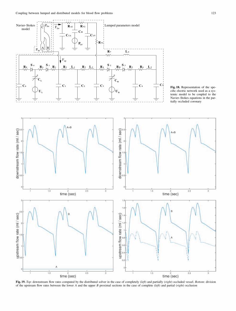
in the previous case. By the way, notice that in the anasto-mosis zone, velocity recirculation arises in the completelyoccluded vessel, while no recirculation is observed in the par-tially occluded one. As it is well known, recirculation zonesare often related to a further development of pathologies inthe vascular district (see e.g. [6]). The downstream flow ratescomputed by the coupled solver are shown in Fig. 19 (top)for both cases of complete and partial occlusion. By com-paring them with the one shown in Fig. 12, we observe thatthe downstream flow rates are obviously the same in bothcases.

The relevance of these results is not tight to the specifictest case (which is indeed a 2D simplification of a real morph-ology) and to the quantitative determination of the variableinvolved here. What is new is the methodology that we pro-pose. Actually, our heterogeneous numerical coupling allowsa correct determination of the fluid dynamical conditions ofa district of interest accounting for the systemic circulation.Specifically, the quantitative determination of a district of in-terest is obtained without the prescription of any presumedboundary conditions. The interface data for the district of in-terest are computed by the solver on the basis of the lumpedmodel. Indeed, our model relies on a closed loop. For in-stance, in the numerical results illustrated here, we can com-pute the distribution of the upstream fluxes between the twobranches of the anastomosis as a function of the relevance of


the stenosis and of the radius of the by-pass. In particular, theflux computed by the Navier–Stokes system is obviously to-tally carried by the by-pass in the completely occluded case,while in the partially occluded one (with a 60% reductionof the section) about 30% of the flow rate is carried by thestenosed vessel.

The flux distribution is a critical parameter for the under-standing and the design of surgical operations (as in the caseof shunts, see e.g. [2]) and it is very difficult to be correctlyquantified, being extremely sensible to the boundary condi-tions specifications. The prescription of boundary conditionsis therefore a major issue for the reliability of the numericalresults. In this respect, the multiscale heterogeneous numeri-cal model featuring lumped and distributed submodels repre-sents a very effective tool of investigation.

7 Conclusions

In the numerical simulations of blood flow in a specific vas-cular district, the correct prescription of the boundary con-ditions on the “artificial” sections, delimiting the computa-tional domain with respect to the remaining circulation, is

Fig. 14. Velocity contour plots in the totally occluded vessel for differenttimes: a quarter of a beat (top), half a beat (middle) and end of a beat(bottom)

a non trivial task. The specific determination of these condi-tions would account for the multiscale nature of the circula-tory system, where local and global phenomena are strictlyrelated.

Fig. 15. Streamlines in the totally occluded vessel (anastomosis) for differ-ent times: a quarter (top) of a beat, half a beat (middle) and end of a beat(bottom)


Fig. 16. Velocity contour plots in the partially occluded vessel for differ-ent times: a quarter (top) of a beat, half a beat (middle) and end of a beat(bottom)

In this paper, we propose a heterogeneous modelization,where a specific district of interest is described by the classi-cal Navier–Stokes equations for incompressible fluids and the“systemic” side is provided by nonlinear ordinary differentialequations based on an hydraulic/electric analogy. The levelof accuracy of such lumped description of the circulation canbe improved according to the interest of a specific application.The two submodels are then coupled by means of interfaceconditions involving the mean pressures and the flow rates.

The idea of coupling both local and systemic model forthe determination of the boundary conditions to be prescribedfor the local simulation is not new: see e.g. [16]. In thiscase, the boundary data determination is based on the solu-tion of a systemic global network model, that includes thelumped representation of the district of interest and providesa quantitative determination of the boundary conditions forthe local simulation. This approach has the drawback of re-quiring a lumped parameter representation also of the vesselat hand, which is often not available (in the case of com-plex morphologies) and has to be set up again by means ofnumerical simulations. Our approach considers a genuinely

Fig. 17. Streamlines in the partially occluded vessel (anastomosis) for dif-ferent times: a quarter (top) of a beat, half a beat (middle) and end of a beat(bottom)

heterogeneous model, where the distributed and lumped sub-models are really coupled in the same solver. This can bedone, by suitably filling up the gap between the level of de-tail of the lumped and the one of the distributed submodels. In


A B

C Lumped parameters modelmodel

Navier−Stokes

up

P

P

Fdwdw

Fup

U U

C C C C C C


LR

R

RR

CC

8 L 1 2 1 3 2 R 5 6 3

R

R

L

L

A2 V2

V1

7 4

4 1 24

6 1 2 3 4 5

S 3

PLV

H

CA C CV

C C

Fig. 18. Representation of the spe-cific electric network used as a sys-temic model to be coupled to theNavier–Stokes equations in the par-tially occluded coronary

Fig. 19. Top: downstream flow rates computed by the distributed solver in the case of completely (left) and partially (right) occluded vessel. Bottom: divisionof the upstream flow rates between the lower A and the upper B proximal sections in the case of complete (left) and partial (right) occlusion


particular, the numerical treatment of defective boundary con-ditions is based on the variational approach suggested in [8].

The numerical method for the treatment of the heteroge-neous model can be set up with different iterative schemes.In order to safe the computational efficiency, we have pro-posed an explicit coupling, which in our applications turnsout to be stable in the range of the time step size requiredby the Navier–Stokes solver. Numerical results on analyticalcases provide the expected degree of accuracy. On test casesof physiological interest, the proposed numerical scheme al-lows the accurate determination of local blood flow features(recirculation zones, etc.) and the determination of relevantparameters such as the flux splitting between the differentbranches.

The presented model, successfully adopted on 2D cases, isgoing to be extended to 3D ones obtained by the modelling ofreal geometries (see [2], [3]).

Acknowledgements. The authors wish to thank Prof. R. Pietrabissa, Eng.G. Dubini and Eng. F. Migliavacca for many fruitful discussions and forhaving kindly provided the lumped systemic network used in our numericalsimulations.

References

1. Archie, J.P., Feldtman, R.P.: (1981) Critical stenosis of the internalcarotid artery. Surgery 89(1), 67–70 (1981)

2. Dubini, G., Migliavacca, F., Pietrabissa, R., Quarteroni, A., Ragni, S.,Veneziani, A.: From the global cardiovascular system hemodynamicsdown to the local blood motion: preliminary applications of a multi-scale approach. Proceedings of European Congress on ComputationalMethods in Applied Sciences and Engineering – ECCOMAS 2000,Barcelona, September 2000

3. Laganà, K., Dubini, G., Migliavacca, F., Pietrabissa, R., Pennati, G.,Veneziani, A., Quarteroni, A.: Multiscale modelling as a tool to pre-scribe realistic boundary conditions for the study of surgical proced-ures. to appear in Biorheology (2001)

4. Fogliardi, R., Burattini, R., Shroff, S.G., Campbell, K.B.: Fit to diastolicarterial pressure by third order lumped model yields unreliable estimatesof arterial compliance. Med. Eng. Phys. 18(3), 225–233 (1996)

5. Formaggia, L., Nobile, F., Quarteroni, A., Veneziani, A.: Multiscalemodelling of the circulatory system: a preliminary analysis. Comp.Vis. Science 2(2-3), 75–83 (1999)

6. Friedman, M.H., Deters, O., Bargeron, C., Hutchins, G.M., Mark, F.:Shear-dependent thickening of the human arterial intima. Arterioscle-rosis 9, 511–522 (1989)

7. Heywood, J., Rannacher, R.: Finite element approximation of the nonstationary Navier–Stokes problem. Part I. Regularity of solutions andsecond order error estimates for spatial discretization. SIAM J. Numer.Anal. 19, 275–311 (1982)

8. Heywood, J., Rannacher, R., Turek, S.: Artificial boundaries and fluxand pressure conditions for the incompressible Navier–Stokes equa-tions. Int. J. Num. Meth. Fl. 22, 325–352 (1996)

9. Hoppensteadt, F., Peskin, C.: Mathematics in medicine and the life sci-ences. Texts in Applied Mathematics. Berlin, Heidelber, New York:Springer 1992

10. Inzoli, F., Migliavacca, F., Mantero, S.: Pulsatile flow in an aorto-coronary bypass 3-D model. Biofluid Mechanics Proceedings of the3rd International Symposium, July 16–19, Prof. D. Liepsch (ed.), Mu-nich, Germany 1994

11. Karlin, V.: Numerical algorithms for flows in nodes of 2-D modelof pipe networks. School of Mechanical and Offshore EngineeringSchoolhill Aberdeen – Preprint

12. McDonald, D.: Blood flow in arteries. Third edition ed. by W. Nicholsand M.F. O’Rourke. London: Edward Arnold Ltd. 1990

13. Noordergraaf, A., Boom, H., Verdouw, P.: A human systemic analogcomputer. In: Noordergraaf, A. (ed): 1st Congr. Soc. for Ballistocar-diographic res. p. 23. 1960

14. Olufsen, M.S.: Structured tree outflow condition for blood flow inlarger systemic arteries. Am. J. Phys. 276, H257–H268 (1999)

15. Palladino, J.L., Mulier, J.P., Noordergraaf, A.: Closed-loop circulationmodel based on the Frank mechanism. Surveys on Mathematics forIndustry 7(3), 177–186 (1997)

16. Pennati, G., Migliavacca, F., Dubini, G., Pietrabissa, R., Leval, M.R. de:A mathematical model of circulation in the presence of the bidirec-tional cavopulmonary anastomosis in children with a univentricularheart. Med. Eng. Phys. 19(3), 223–234 (1997)

17. Perktold, K., Resch, M., Florian, H.: Pulsatile Non-Newtonian flowcharacteristics in a three-dimensional human carotid bifurcationmodel, ASME J. Biomech. Eng. 113, 463–475 (1991)

18. Quarteroni, A., Ragni, S., Veneziani, A.: Existence of a solution forproblems coupling lumped and distributed blood flow models. In prep-aration. (2001)

19. Quarteroni, A., Sacco, R., Saleri, F.: Numerical Mathematics. Texts inAppl. Math. 37, (2000)

20. Quarteroni, A., Valli, A.: Domain Decomposition Methods for PartialDifferential Equations. Oxford: Oxford University Press 1999

21. Quarteroni, A., Saleri, F., Veneziani, A.: Factorization methods for thenumerical approximation of Navier–Stokes equations. Comp. Meth.Appl. Mech. Eng. 188, 505–526 (2000)

22. Quarteroni, A., Tuveri, M., Veneziani, A.: Computational vascularfluid dynamics: problems, models and methods. Comp. Vis. Science2(4), 163–197 (2000)

23. Ragni, S.: Multiscale modelling of the circulatory system. Ph. D. The-sis. Università di Milano 2000

24. Rideout, V.C., Dick, D.E.: Difference-differential equations for fluidflow in distensible tubes. IEEE Transactions on bio-medical engineer-ing BME-14(3), 171–177 (1967)

25. Sagawa, K., Suga, H., Nakayama, K.: Instantaneous pressure–volumeratio of the left ventricle versus instantaneous force–length relation ofpapillary muscle. In: Baan, J., Noordergraaf, A., Raines, J. (eds.): Car-diovascular System Dynamics. pp. 99–105. Cambridge, MA: M.I.T.Press 1978

26. Taylor, C.: A computational framework for vascular disease investiga-tion. PhD thesis. Stanford University 1996

27. Toy, S.M., Melbin, J., Noordergraaf, A.: Reduced models of arterialsystems. IEEE Transactions on Biomedical Engineering BME-32(2),174–176 (1985)

28. Veneziani, A.: Boundary conditions for blood flow problems. Proceed-ings of ENUMATH 97 (Heidelberg). pp. 596–605. River Edge, NJ:World Sci. Publishing 1998

29. Veneziani, A.: Mathematical and numerical modelling of blood flow.PhD thesis. Università di Milano 1998

30. Westerhof, N., Bosman, F., De Vries, C.J., Noordergraaf, A.: Analogstudies of the human systemic arterial tree. J. Biomechanics 2, 121–143 (1969)

31. Womersley, J.: Method for the calculation of velocity rate of flow andviscous drag in arteries when the pressure gradient is known. J. Phys-iol. 127, 553–563 (1955)

32. Xie, W.: Integral representations and L∞ bounds for solutions of theHelmholtz equation on arbitrary open sets in R2 and R3. Diff. Int.Eqn. 8, 689–698 (1995)

33. Zeidler, E.: Nonlinear functional analysis and its applications: 1. fixed-point theorems. Berlin, Heidelberg, New York: Springer 1986

Documents

Coupling between lumped and distributed models for blood flow problems