Embed Size (px)
Citation preview
University of Central Florida University of Central Florida
STARS STARS
Electronic Theses and Dissertations, 2004-2019
2012
Coupled Usage Of Discrete Hole And Transpired Film For Better Coupled Usage Of Discrete Hole And Transpired Film For Better
Cooling Performance Cooling Performance
Michael Torrance University of Central Florida
Part of the Mechanical Engineering Commons
Find similar works at: https://stars.library.ucf.edu/etd
University of Central Florida Libraries http://library.ucf.edu
This Masters Thesis (Open Access) is brought to you for free and open access by STARS. It has been accepted for
inclusion in Electronic Theses and Dissertations, 2004-2019 by an authorized administrator of STARS. For more
information, please contact [email protected].
STARS Citation STARS Citation Torrance, Michael, "Coupled Usage Of Discrete Hole And Transpired Film For Better Cooling Performance" (2012). Electronic Theses and Dissertations, 2004-2019. 2391. https://stars.library.ucf.edu/etd/2391

i
COUPLED USAGE OF DISCRETE HOLE AND TRANSPIRED FILM FOR
BETTER COOLING PERFORMANCE
by
MICHAEL C. TORRANCE
B.S. University of Central Florida, 2010
A thesis submitted in partial fulfillment of the requirements
for the degree of Master of Science in Mechanical Engineering
in the Department of Mechanical, Material, and Aerospace Engineering
in the College of Engineering and Computer Science
at the University of Central Florida
Orlando, Florida
Summer Term
2012
Major Professor: Jay Kapat

ii
© 2012 MICHAEL C. TORRANCE
iii
ABSTRACT
Electricity has become so ingrained in everyday life that the current generation has no
knowledge of life without it. The majority of power generation in the United States is the result
of turbines of some form. With such widespread utilization of these complex rotating machines,
any increase in efficiency translates into improvements in the current cost of energy. These
improvements manifest themselves as reductions in greenhouse emissions or possible savings to
the consumer.
The most important temperature regarding turbine performance is the temperature of the
hot gas entering the turbine, denoted turbine inlet temperature. Increasing the turbine inlet
temperature allows for increases in power production as well as increases in efficiency. The
challenge with increasing this temperature, currently the hottest temperature seen by the turbine,
is that it currently already exceeds the melting point of the metals that the turbine is
manufactured from. Active cooling of stationary and rotating components in the turbine is
required. Cooling flows are taken from bleed flows from various stages of the compressor as
well as flow from the combustor shell. This cooling flow is considered wasted air as far as
performance is concerned and can account for as much as 20% of the mass flow in the hot gas
path. Lowering the amount of air used for cooling allows for more to be used for performance
gain.
Various technologies exist to allow for greater turbine inlet temperatures such as various
internal channel features inside of turbine blades, film holes on the surface to cool the outside of
the airfoil as well as thermal barrier coatings that insulate the airfoils from the hot mainstream

iv
flow. The current work is a study of the potential performance impact of coupling two effusion
technologies, transpiration and discrete hole film cooling. Film cooling and transpiring flows are
individually validated against literature before the two technologies are coupled. The coupled
geometries feature 13 film holes of 7.5mm diameter and a transpiring strip 5mm long in the
streamwise direction. The first coupled geometry features the porous section upstream of the film
holes and the second features it downstream. Both geometries use the same crushed aluminum
porous insert of nominal porosity of 50%. Temperature sensitive paint along with an ‘adiabatic’
Rohacell surface (thermal conductivity of 0.029W/m-K) are used to measure adiabatic film
cooling effectiveness using a scientific grade high resolution CCD camera. The result is local
effectiveness data up to 50 film hole diameters downstream of injection location. Data is laterally
averaged and compared with the baseline cases. Local effectiveness contours are used to draw
conclusions regarding the interactions between transpiration and discrete hole film cooling. It is
found that a linear superposition method is only valid far downstream from the injection
location. Both coupled geometries perform better than transpiration or the discrete holes far
downstream of the injection location. The coupled geometry featuring the transpiring section
downstream of the film holes matches the transpiration effectiveness just downstream of
injection and surpasses both transpiration and film cooling further downstream.

v
Dedicated to Tricia,
You kept me going and made it all worth it.

vi
ACKNOWLEDGMENTS
This work would not have been possible without the help of my advisor Dr. Jay Kapat
and the help from my colleagues at the CATER lab. Special thanks go to Greg Natsui and
Roberto Claretti, none of this would have been possible without your dedication and hard work.
Additional mention goes to Perry Johnson and Mark Miller.
To those still at the CATER lab, study hard, find the topic you are interested in, and
become the expert. I can’t thank the people at the lab enough starting from all the way back in
2010 with Carson showing me how to weld thermocouples. I learned so many real world
applicable things which you just will not learn in the classroom.
Additional thanks goes to my colleagues at Siemens, Dr. Michael Crawford, Glenn
Brown, Ken Landis, and Dr. Ching-Pang Lee. I benefitted greatly from the knowledge and
experience imparted from you. The projects we did for Siemens were what pushed us to do
excel.
Those at the lab during my time there, Bryan, Michelle, Anthony, Matt, Lucky, Greg,
Roberto and all the others, thank you for being my friends and being so awesome to work with.
I’d like to thank Dr. Vasu and Dr. Xu for being on my thesis committee. My time at UCF
has taught me a great deal and it has been worth it.

vii
Finally, I would like to thank my family for their continued support and understanding. I
couldn’t have done this without the guidance from my brother and having someone that could
answer difficult questions. Lastly, thank you Tricia for putting up with me these last months. I
know it has been difficult.

viii
TABLE OF CONTENTS
LIST OF FIGURES ........................................................................................................................ x
LIST OF TABLES ........................................................................................................................ xv
NOMENCLATURE .................................................................................................................... xvi
CHAPTER 1: INTRODUCTION .................................................................................................. 1
Turbomachinery ........................................................................................................................................ 1
Film Cooling ............................................................................................................................................... 5
Transpiration Cooling ................................................................................................................................ 6
Current Work ............................................................................................................................................ 6
CHAPTER 2: BACKGROUND .................................................................................................... 9
Film Cooling ............................................................................................................................................... 9
Film Cooling Nomenclature .................................................................................................................... 11
Single Row Film Cooling .......................................................................................................................... 14
Full Coverage Film Cooling ...................................................................................................................... 19
Transpiration ........................................................................................................................................... 21
CHAPTER 3: NUMERICAL PREDICTIONS ............................................................................ 26
First Order Analysis Domain ................................................................................................................... 26
Predicting Mass Flow .............................................................................................................................. 28
Predicting Effectiveness .......................................................................................................................... 29
Predicting Aerodynamic Losses .............................................................................................................. 29
Predicting Thermo-Mechanical Stresses ................................................................................................. 30
Coupled Geometries ............................................................................................................................... 39
Finalized Geometries .............................................................................................................................. 41
CHAPTER 4: EXPERIMENTAL SETUP ................................................................................... 44

ix
Wind Tunnel ............................................................................................................................................ 44
Hot-wire Anemometry ............................................................................................................................ 46
Turbulence Length Scale ..................................................................................................................... 48
Transpiration Numerical Study ............................................................................................................... 50
Grid Independence ............................................................................................................................. 52
Film Cooling Effectiveness ...................................................................................................................... 54
Experimental Geometries ....................................................................................................................... 55
Temperature Sensitive Paint ................................................................................................................... 58
Film Cooling Effectiveness Data Reduction............................................................................................. 61
Experimental Uncertainty ....................................................................................................................... 62
CHAPTER 5: EXPERIMENT RESULTS.................................................................................... 65
Jet Lateral Profiles ................................................................................................................................... 65
Turbulence Length Scale ..................................................................................................................... 76
Transpiration Numerical Results ............................................................................................................. 78
Experimental Validation .......................................................................................................................... 80
Discrete Hole Film Cooling .................................................................................................................. 81
Transpiration Cooling ........................................................................................................................ 104
Transpiration Numerical Versus Experimental ..................................................................................... 110
Multi-Row Results ................................................................................................................................. 113
Coupled – B Results ............................................................................................................................... 120
Coupled – A Results .............................................................................................................................. 128
Coupled Comparison ............................................................................................................................. 134
CHAPTER 6: CONCLUSION ................................................................................................... 136
Ex Supra................................................................................................................................................. 136
De Futuro .............................................................................................................................................. 137
REFERENCES ........................................................................................................................... 138

x
LIST OF FIGURES
Figure 1: Assembled Gas Turbine Rotor ........................................................................................ 2
Figure 2: Open Loop Brayton Cycle ............................................................................................... 3
Figure 3: Brayton Cycle T-S Diagram - Ideal and With Inefficiencies .......................................... 3
Figure 4: Counter-Rotating Vortex Pair ....................................................................................... 10
Figure 5: Film Cooling Nomenclature .......................................................................................... 12
Figure 6: Laterally averaged effectiveness trend with density ratio at M=1.0 ............................. 16
Figure 7: Geometrical Description ................................................................................................ 20
Figure 8: Effectiveness Trend ....................................................................................................... 22
Figure 9: Numerical Domain ........................................................................................................ 26
Figure 10: Transpiration Analytical Results ................................................................................. 32
Figure 11: Discrete Hole Film Cooling Analytical Results .......................................................... 34
Figure 12: (Top) Offset Analysis, (Bottom) Effectiveness Contours ........................................... 36
Figure 13: Effect of Blowing Ratio .............................................................................................. 37
Figure 14: Effect of P/D and h/D .................................................................................................. 38
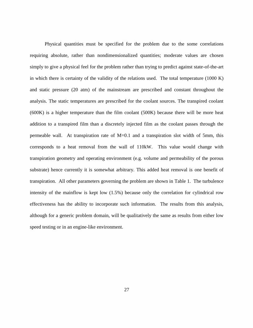
Figure 15: Baseline Geometries. (a) Cylindrical Row, (b) Transpiration Section........................ 42
Figure 16: Coupled Geometries. (a) Transpiration Upstream, (b) Transpiration Downstream,
dimensions in mm. ........................................................................................................................ 43
Figure 17: Experimental Apparatus .............................................................................................. 44
Figure 18: (a) Plenum Setup, (b) Transpiration Coupon .............................................................. 46
Figure 19: Computational Domain ............................................................................................... 51

xi
Figure 20: The converging GCI indices for 20 point monitors .................................................... 53
Figure 21: Test geometries, from top; [30/0/14], [30/45/14], [30/0/7], [90/0/1] .......................... 57
Figure 22: Jablonski Energy-Level Diagram ................................................................................ 59
Figure 23: Calibration Curve ........................................................................................................ 60
Figure 24: Effectiveness Uncertainty Tree ................................................................................... 62
Figure 25: Hot-wire Traverse Locations ....................................................................................... 65
Figure 26: Slot Jet Lateral Traverse Velocities............................................................................. 66
Figure 27: Slot Jet Turbulence Intensities .................................................................................... 67
Figure 28: 0.6 Porosity Lateral Traverse Velocities ..................................................................... 68
Figure 29: 0.6 Porosity Turbulence Intensity ............................................................................... 69
Figure 30: 0.5 Porosity Lateral Traverse Velocities ..................................................................... 71
Figure 31: 0.5 Porosity Lateral Turbulence Intensities ................................................................. 72
Figure 32: 0.4 Porosity Lateral Traverse Velocities ..................................................................... 73
Figure 33: 0.4 Porosity Lateral Turbulence Intensities ................................................................. 74
Figure 34: Autocorrelation at 0.4 porosity jet centerline .............................................................. 75
Figure 35: Power Spectral Density 0.4 porosity ........................................................................... 76
Figure 36: Transpiration CFD Laterally Averaged Effectiveness ................................................ 79
Figure 37: Difference in Effectiveness from Case1 ...................................................................... 80
Figure 38: Laterally average effectiveness M=0.5 ....................................................................... 83
Figure 39: Laterally Averaged Film Effectiveness at M=1.0 ....................................................... 85
Figure 40: Laterally Averaged Film Effectiveness at M=2.0 ....................................................... 86
Figure 41: Laterally Averaged Film Effectiveness at M=0.4 ....................................................... 87

xii
Figure 42: Laterally Averaged Film Effectiveness at M=0.8 ....................................................... 88
Figure 43: Laterally Averaged Film Effectiveness at M=1.2 ....................................................... 89
Figure 44: Centerline Film Effectiveness at M=0.5 ..................................................................... 91
Figure 45: Centerline Film Effectiveness at M=1.0 ..................................................................... 92
Figure 46: Centerline Film Effectiveness at M=2.0 ..................................................................... 93
Figure 47: Centerline Film Effectiveness ..................................................................................... 94
Figure 48: Laterally Averaged Effectiveness ............................................................................... 95
Figure 49: Local Film Effectiveness Contours M=0.4 ................................................................. 96
Figure 50: Local Film Effectiveness Contours M=0.5 ................................................................. 97
Figure 51: Local Film Effectiveness Contours M=0.8 ................................................................. 98
Figure 52: Local Film Effectiveness Contours M=1.0 ................................................................. 99
Figure 53: Lateral Variation of Film Effectiveness M=1.0 ........................................................ 100
Figure 54: Spanwise Local Effectiveness Trace Location .......................................................... 101
Figure 55: Streamwise Average Diagram ................................................................................... 102
Figure 56: Local Film Effectiveness Contours M=1.2 ............................................................... 102
Figure 57: Local Film Effectiveness Contours M=2.0 ............................................................... 103
Figure 58: Transpiration Film Effectiveness M=0.05 ................................................................ 105
Figure 59: Transpiration Film Effectiveness M=0.10 ................................................................ 106
Figure 60: Transpiration Film Effectiveness M=0.15 ................................................................ 107
Figure 61: Transpiration Film Effectiveness, Log-Log .............................................................. 108
Figure 62: Transpiration Laterally Averaged Effectiveness ....................................................... 109
Figure 63: Centerline Transpiration Effectiveness ..................................................................... 110

xiii
Figure 64: CFD Versus Experimental Laterally Averaged Effectiveness .................................. 111
Figure 65: [30/45/14] Film Cooling Effectiveness versus Data Reproduced From Mayle ........ 114
Figure 66: [30/0/14] Laterally Averaged Effectiveness .............................................................. 115
Figure 67: Effect of 45° Compound Angle ................................................................................. 116
Figure 68: [30/0/7] Laterally Averaged Effectiveness ................................................................ 117
Figure 69: [90/0/1] Laterally Averaged Effectiveness ................................................................ 118
Figure 70: Multi-Row Geometry Laterally Averaged Effectiveness .......................................... 119
Figure 71: Streamwise Averaged Effectiveness ......................................................................... 120
Figure 72: Mass Flow vs Differential Pressure........................................................................... 121
Figure 73: Local Effectiveness Contours MCYL = 0.41 MTRAN =0.074 ...................................... 122
Figure 74: Local Effectiveness Contours MCYL =0.81 MTRAN=0.075 ........................................ 123
Figure 75: Local Effectiveness Contours MCYL = 1.22 MTRAN =0.21 ........................................ 123
Figure 76: Laterally Averaged Effectiveness Coupled-B ........................................................... 125
Figure 77: Laterally Averaged Effectiveness Comparison, Mcyl=0.4, Mtran=0.07 .................. 126
Figure 78: Laterally Averaged Effectiveness Comparison, Mcyl=0.8, Mtran=0.08 .................. 127
Figure 79: Laterally Averaged Effectiveness Comparison, Mcyl=1.2, Mtran=0.21 .................. 128
Figure 80: Laterally Averaged Effectiveness Coupled-A ........................................................... 129
Figure 81: Local Effectiveness Contours MCYL = 0.4 MTRAN =0.11 .......................................... 130
Figure 82: Local Effectiveness Contours MCYL = 0.8 MTRAN =0.12 .......................................... 130
Figure 83: Local Effectiveness Contours MCYL = 1.2 MTRAN =0.22 .......................................... 131
Figure 84: Laterally Averaged Effectiveness Comparison, MCYL=0.4, MTRAN=0.11 ................. 132
Figure 85: Laterally Averaged Effectiveness Comparison, MCYL=0.8, MTRAN=0.12 ................. 133

xiv
Figure 86: Laterally Averaged Effectiveness Comparison, MCYL=1.2, MTRAN=0.22 ................. 134
Figure 87: Laterally Averaged Effectiveness Coupled Geometries ........................................... 135

xv
LIST OF TABLES
Table 1: Design Parameters .......................................................................................................... 28
Table 2: Cylindrical Hole Parameters ........................................................................................... 39
Table 3: Transpiration Parameters ................................................................................................ 40
Table 4: Coupled Geometries ....................................................................................................... 41
Table 5: Hot-Wire Test Parameters .............................................................................................. 47
Table 6: Multi-Row Geometries ................................................................................................... 56
Table 7: Turbulence Length Scales ............................................................................................... 77
Table 8: CFD Case Description .................................................................................................... 78
Table 9: Validation Cases ............................................................................................................. 82
Table 10: Area Averaged Effectiveness ..................................................................................... 112

xvi
NOMENCLATURE
A – Area [m2]
α – Film cooling hole inclination angle [°]
β – Film cooling hole compound angle [°]
C – Constant
CFD – Computational Fluid Dynamics
Cd – Discharge coefficient [-]
D – Jet hole diameter [m]
DR – Density ratio [-]
E – Energy spectra from streamwise velocity
η – Film cooling effectiveness [-]
h – Length of transpiring surface in flow direction
htc – Heat transfer coefficient [W/m2K]
θ – Dimensionless wall temperature [-]
I – Momentum flux ratio [-]
I/Iref – Intensity ratio, with respect to TSP images

xvii
k – Thermal conductivity [W/mK]
kf – Thermal conductivity of fluid [W/mK]
L – Length of film cooling hole [m]
LI – Turbulent Length Scale based on autocorrelation
LII – Turbulent Length Scale based on zero frequency energy spectrum
M – Blowing ratio or mass flux ratio [-]
– Mass flow rate [kg/s]
μ – Dynamic viscosity [N*s/m2]
NuD – Nusselt number based on jet diameter [-]
n – Row number
ν – Kinematic viscosity [m2/s]
ξ – Unheated starting length [m]
p – Pressure [N/m2]
q – Heat flow rate [W]
q” – Heat flux [W/m2]
r – Radial coordinate
xviii
R11 – Autocorrelation Coefficient (X direction)
Re – Reynolds number [-]
s – Entropy [J/K]
T – Temperature [K]
t – Thickness of wall [m]
TKE – Turbulent Kinetic Energy = (u’2
+ v’2
+ w’2)1/2
Tu – Turbulence Intensity = v’/V
U – Velocity [m/s]
U, V, W – Mean velocity, stream, normal, lateral component [m/s]
u’, v’, w’ – Velocity fluctuation, stream, normal, lateral component [m/s]
VD – Darcy (Superficial) Velocity = Q/(ρAslot) [m/s]
X – streamwise hole spacing [m]
Y – Wall normal distance[m]
Z – Spanwise hole spacing[m]
Subscripts
aw – Adiabatic wall

xix
c – Coolant
f – With film
h – Slot width
m – Mainstream
0 – Without film
w – Wall

1
CHAPTER 1: INTRODUCTION
Turbomachinery
Turbomachinery is defined as the mechanical system responsible for the transfer of
energy from a fluid utilizing a rotor. This transfer of energy is the fundamental basis for power
generation. Through turbomachines, power is generated, airplanes are flown, and marine vessels
are propelled. Hydrocarbon fuels are the primary mode of energy generation and due to the
increase in public awareness of the environmental and economic impact of burning hydrocarbon
fuels, it is crucial to extract as much power from each pound of fuel as possible with the least
amount of released pollution. With the push towards new "green" technologies, it is crucial to
not forget that the old concepts are still being developed and improved in power output and
efficiency.

2
Figure 1: Assembled Gas Turbine Rotor
Turbines are responsible for nearly the entirety of power generation in the United States.
The fundamental thermodynamic operation of gas turbines is the Brayton cycle. In the ideal open
loop Brayton cycle, air is isentropically compressed in a compressor, heat is added to the air
under constant pressure through the combustors, and power is extracted through the isentropic
expansion of the air through the turbine. Figure 2 is a diagram of the open loop Brayton cycle.
The Brayton cycle represented on a T-S diagram with and without losses is shown in Figure 3.

3
Figure 2: Open Loop Brayton Cycle
Figure 3: Brayton Cycle T-S Diagram - Ideal and With Inefficiencies

4
Efficiency of the ideal Brayton cycle is defined using the difference in temperatures in
Equation 1.
(1)
Readily apparent in this equation is the increase in efficiency resulting from increasing
T3 (Turbine Inlet Temperature). It has been argued that this is the most dependable method of
increasing efficiency (Wilcock, Young, & Horlock, 2005).
The Turbine Inlet Temperature (TIT), the hottest temperature experienced outside of
combustion, has exceeded the allowable metal temperatures since the 1960's. Passive cooling is
woefully insufficient for modern turbine blades, therefore active cooling is required. As the TIT
increases, the heat transmitted to the turbine blades is increased. The primary method of cooling
the blades is utilizing air bled before the combustion stage.
Cooling air is fed through internal channels inside the blades and is ejected through
features on the blade surfaces such as discrete holes or slots. The blade cooling system must be
designed to minimize thermal gradients through the blade therefore minimizing thermal stresses.
The blade cooling air is extracted after it has traveled through the entire compressor therefore has
had the maximum amount of work imparted to it. This air is considered the most "expensive";
the utilization of which incurs the greatest thermal efficiency penalty. Therefore minimization of

5
cooling air is crucial for high efficiency (Han, Sandip, & Srinath, 2000). The focus of the current
work is on development of a more efficient implementation of current cooling schemes.
Film Cooling
Discrete hole film cooling is common in usage for turbine blade and vane cooling. The
first stage vane and blade are subjected to the highest heat fluxes downstream of the combustor,
on the order of 1.5-2 MW/m2 (Polezhaev, 1997). Therefore the first stage vane and blade
requires the greatest amount of coolant injection and requires the greatest surface area covered.
Discrete hole film cooling directly protects the surface of the airfoils at discrete locations as well
as downstream of the injection point (Han et al., 2000). The internal channels created through the
airfoil surface are additionally cooled by internal convection.
Showerhead cooling consists of multiple rows of closely space holes near the stagnation
point of the airfoil. Areas of high thermal gradients on the pressure and suction sides of the
airfoil can be cooled with single or multiple rows of film holes. Due to the non-uniformity of
heat flow rate along the contour of the airfoil, cooling schemes are not symmetrical. The design
of a film cooling system relies on knowledge of airfoil temperatures consequently "blade life
may be reduced by half if the blade metal temperature prediction is off by 50°F” (Han et al.,
2000). Additionally, detrimental thermal gradients can be created downstream of injection
locations from the unprotected surface between film jets. However, film cooling is a widely
adopted method of cooling as opposed to transpiration cooling.

6
Transpiration Cooling
Injection through a porous medium is denoted transpiration cooling. The coolant passing
through the pores contributes to the cooling process by absorbing some of the internal energy of
the airfoil as well as simultaneously decreasing the convective heat transfer on the exterior of the
airfoil (Polezhaev, 1997). The exiting flow from the porous surface drives the hot gas boundary
layer off of the airfoil surface and coats the downstream region with a lower temperature fluid.
The result is a decrease in heat transfer rate to the surface. Transpiration cooling is the limiting
case of film cooling where the pitch to diameter ratio is taken to unity (Eckert & Cho, 1994).
Transpiration has been researched since the 1950's (Kays, 1972) and yet it is still not in common
usage in production components due to structural and manufacturing difficulties. With the
technological advancement of laser techniques such as laser additive manufacturing (LAM),
porous sections will be able to be created simultaneously with the entire airfoil in a single step
process. Implementation of these manufacturing techniques is in the foreseeable future and could
allow transpiration to be finally utilized in airfoils.
Current Work
The purpose of this study is to investigate the cooling performance of coupling of discrete
hole film cooling and transpiration cooling. Experimental data is greatly lacking for transpiration
cooling and although film cooling is a widely researched topic, no data coupling the two can be
found in literature. By conducting this study, the body of knowledge in open literature is
expanded.

7
With the absence of coupled data available in literature, an educated starting point had to
be formulated. It has been shown that film cooling performance of multiple rows of discrete
holes can be predicted using the data from a single row of holes through superposition (Sellers,
1963). Discrete hole film cooling data and transpiration cooling data is separately available in
open literature. Two baseline geometries are experimentally characterized, one purely discrete
hole film cooling and one purely transpiration cooling. Boundary conditions for the transpiring
flow were established utilizing hot-wire anemometry. The turbulence length scale described by
Barrett and Hollingsworth (2001) was utilized which allowed for the length scale to be computed
from a single location. Integral time scales were calculated using the zero-frequency estimate of
the one dimensional energy spectrum (Lewalle & Ashpis, 2004). The implications of this
information are to provide more accurate boundary conditions used for computational fluid
dynamic analysis of transpired flow from similar geometries. A computational fluid dynamic
study was performed to evaluate those boundary conditions without modeling the porous wall.
Multiple rows of discrete holes and multiple rows of discrete transpiration slots are
investigated for the purpose of comparison for the coupled geometries. Different configurations
of hole spacing along with compound angle are investigated in order to compare cooling
performance to the multiple row transpiration case. Four multi-row configurations are tested
experimentally using high resolution measurements of Temperature Sensitive Paint (TSP).
Through the analytical simulation, the critical features of the coupled geometry are
identified, along with the relative sensitivity of those features to the cooling effectiveness and
aerodynamic losses. In this study geometries were restricted such that separately the discrete hole

8
film cooling and transpiration cooling could be validated with available data. Two coupled
geometries are tested experimentally using high resolution TSP measurements. The
experimentally obtained surface data is used to characterize the performance of the two coupled
geometries.
Adiabatic film cooling effectiveness data is presented for a total of eight different
geometries. The geometries range from some which are comparable to literature and some that is
completely novel. The advantages of coupling discrete hole film cooling and transpiration
cooling could favorably influence further cooling designs.

9
CHAPTER 2: BACKGROUND
Film Cooling
Fluid injection has been utilized in a multitude of fields such as rocket nozzles, reentering
space vehicles, plasma jets, and high temperature turbine parts. The body of knowledge is vast
with publications dating more than half a century ago. The focus of film cooling research is to
minimize coolant usage with the maximum amount of surface protected. Early investigations
found that film cooling through a continuous slot was the most effective. Structural
considerations prohibit the usage of large slots which gives rise to the preference of rows of
holes (Goldstein, 1971). The film cooling reference by Goldstein provides an overview of the
early investigations in film cooling for slots and discrete holes. Single hole studies evolved into
single row studies, creating the most basic form of discrete hole film cooling; the row of
cylindrical holes in a flat plate. One of the earlier studies by Bergeles investigated an inclined
cylindrical hole injecting into a crossflow. It was found that the jet lifts off the surface and
penetrates the crossflow boundary layer as the mass flux ratio of coolant to crossflow is
increased (Bergeles, Gosman, & Launder, 1977). The interaction between the crossflow and the
jet flow create counter-rotating vortices that promote crossflow entrainment and jet lift-off
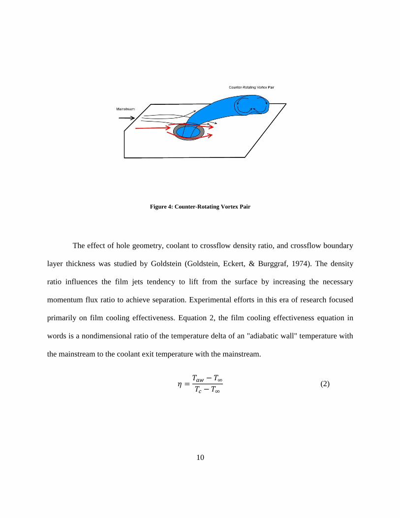
(Haven & Kurosaka, 1997), as shown in Figure 4.
10
Figure 4: Counter-Rotating Vortex Pair
The effect of hole geometry, coolant to crossflow density ratio, and crossflow boundary
layer thickness was studied by Goldstein (Goldstein, Eckert, & Burggraf, 1974). The density
ratio influences the film jets tendency to lift from the surface by increasing the necessary
momentum flux ratio to achieve separation. Experimental efforts in this era of research focused
primarily on film cooling effectiveness. Equation 2, the film cooling effectiveness equation in
words is a nondimensional ratio of the temperature delta of an "adiabatic wall" temperature with
the mainstream to the coolant exit temperature with the mainstream.
(2)

11
Film Cooling Nomenclature
The adiabatic wall temperature is the imaginary quantification of temperature which the
wall assumes when the heat flux from the cooled surface to the interior of the wall is zero. The
film cooling effectiveness is essentially a nondimensionalized form of the adiabatic wall
temperature with the useful properties of readily bounding the possible outcomes of cooling. An
effectiveness of zero represents a wall temperature equal to the crossflow temperature which
corresponds to insufficient cooling. Conversely an effectiveness of unity is the upper limit of
cooling capabilities; the wall temperature is equal to the exiting coolant temperature. The other
property commonly sought after in film cooling investigations is the heat transfer coefficient
(htc).
(3)
The heat flux is represented by q, Taw is the adiabatic wall temperature, and Tw is the wall
temperature. The heat transfer coefficient, also known as convection conductance, must be
known for a total overview of cooling performance. However heat transfer coefficients are not in
the scope of the current study and will not be discussed further.
Film cooling geometries are characterized by nondimensionalizing the various
parameters by the hole diameter.
12
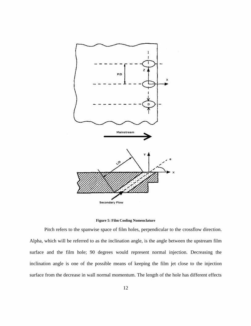
Figure 5: Film Cooling Nomenclature
Pitch refers to the spanwise space of film holes, perpendicular to the crossflow direction.
Alpha, which will be referred to as the inclination angle, is the angle between the upstream film
surface and the film hole; 90 degrees would represent normal injection. Decreasing the
inclination angle is one of the possible means of keeping the film jet close to the injection
surface from the decrease in wall normal momentum. The length of the hole has different effects
13
depending on whether the L/D is considered long or short. A short L/D acts to increase the
effective inclination angle, subsequently increasing wall normal momentum and achieving jet
lift-off at a lower momentum ratio (Sinha, Bogard, & Crawford, 1991).
(4)
(5)
(6)
(7)
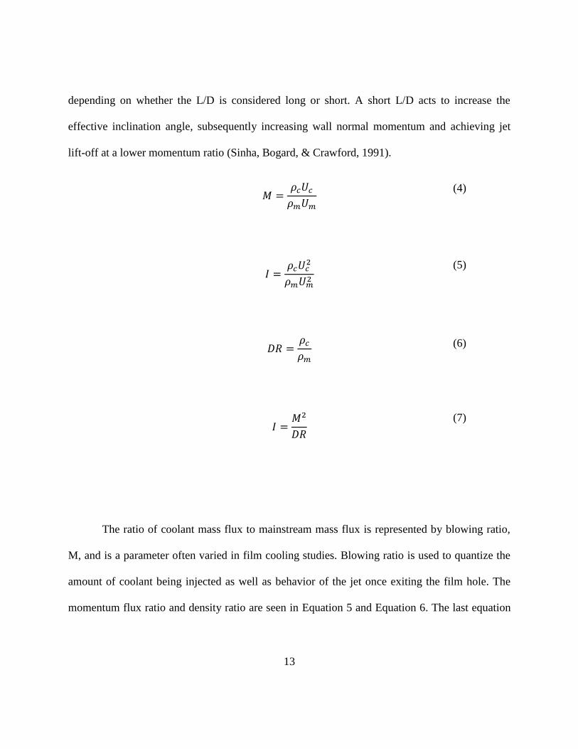
The ratio of coolant mass flux to mainstream mass flux is represented by blowing ratio,
M, and is a parameter often varied in film cooling studies. Blowing ratio is used to quantize the
amount of coolant being injected as well as behavior of the jet once exiting the film hole. The
momentum flux ratio and density ratio are seen in Equation 5 and Equation 6. The last equation

14
relates the momentum flux ratio with the blowing ratio and density ratio. All three ratios are
required to predict the behavior of a film jet.
Single Row Film Cooling
The density ratios typically used in research are typically less than unity; a turbine blade
film cooling scenario would see a density ratio on the order of two. Experimentally it is easier to
create a heated coolant with an approximately ambient mainstream, thus creating the low density
ratio. The effect of density ratio has been studied extensively in (Forth, Loftus, & Jones, 1985;
Goldstein, Jin, & Olson, 1999; Pedersen, Eckert, & Goldstein, 1977; Pietrzyk, Bogard, &
Crawford, 1990). Low density ratios have been shown to induce jet lift off at a lower mass flux
ratio. Logically this makes perfect sense. Assuming a constant mass flow rate through the film
holes, as the density decreases, the velocity must increase. Since the momentum of the film jet
relies on the square of the velocity, the increase in velocity overpowers the decrease in density
and the momentum is increased. The inverse occurs with higher density ratios, the net effect is
for the jets to stay attached to the surfaces. Pedersen et al. (1977) varied the density ratio without
changing the coolant temperature by using a mass transfer analogy and changing the gas used for
the injected coolant. Centerline effectiveness and laterally averaged effectiveness is given at
varying blowing and density ratios for a single row of inclined holes. Equation 8 represents the
lateral average of the film cooling effectiveness.

15
∫
(8)
Laterally averaging the effectiveness allows the spanwise effectiveness distribution to be
averaged and collapsed to single points at increasing downstream positions.
Pedersen et al. (1977) found that at the lowest blowing ratio of 0.213 the change in
density ratio has very little effect. However at the higher blowing ratio of 0.515, increasing the
density ratio equals an increase in effectiveness downstream of injection. The two higher
blowing ratio plots demonstrate the jet attachment effect of higher density ratios. The trend of
decreasing effectiveness with increasing density ratio at a blowing ratio of approximately 1.0 is
shown in Figure 6. As the density ratio increases at constant blowing ratio, a critical value were
the jet detaches from the surface is reached. This shows that when comparing film cooling
effectiveness, nearly equal density ratios must be considered solely. The less than unity density
ratios exhibit markedly lower effectiveness at blowing ratios greater than or equal to 0.515. At a
blowing ratio of 1.05 and 1.96 both density ratio 0.743 and 0.956 show jet lift off downstream of
injection, characterized by the low effectiveness.

16
Figure 6: Laterally averaged effectiveness trend with density ratio at M=1.0
The very long L/D used by Pedersen et al. (1977) was shown by Goldstein (1999) to not
have a significant effect on laterally averaged effectiveness. Goldstein used a naphthalene
sublimation mass transfer technique to measure film effectiveness and heat transfer coefficients.
At the density ratio of unity used by Goldstein et al. (1999), the jet spreading is shown to
decrease as the blowing ratio is increased from 0.5 to 1.0 due to the lift off of the jet. At a
blowing ratio of 2.0, the jet lift off is significant; effectiveness is increased in between the holes
due to the secondary flow turbulently mixing with the mainstream.
Several studies approximately match the geometry used by Pedersen et al. (1977) and
Goldstein et al. (1999), such as those by Brown and Saluja (1979), Foster and Lampard (1980),
Pietrzyk, Bogard, and Crawford (1989); Pietrzyk et al. (1990), and Sinha et al. (1991). Brown
and Saluja (1979) studied a single row of holes at P/D of 2.67 with an inclination of 30 degrees.
Raising the freestream turbulence intensity was found to decrease effectiveness at an X/D of 5,
but at X/D of 15 it increased the effectiveness for blowing ratios greater than 0.7. For lower

17
blowing ratios, the higher turbulence intensity also decreased the effectiveness at X/D of 15. The
turbulence intensity was increased up to a maximum of 12%; the majority of the presented data
was at 1.7% however. The density ratio of 1.1 allows for lower momentum flux ratios which
increases effectiveness for higher blowing ratios compared to low density ratio studies. The
increase in effectiveness by higher turbulence intensities for higher blowing ratios is due to the
increased jet spreading of the lifted off jet. However the increased jet spreading comes at the cost
of higher jet lift off closer to the hole exit.
The effect of injection angle, upstream boundary layer thickness, and hole spacing was
studied by Foster and Lampard (1980). At low blowing rates, the effectiveness is increased by
low inclination angles; however the trend reversal is due to jet lift off. At the higher blowing
rates, the low inclination angle jets lift from the surface and penetrate further into the mainstream
than the higher and normal injection cases. The normal injection case has the highest wall normal
velocity, but the jet spreads immediately and subsequently stays closer to the surface. When the
jets lift off the mainstream enters the region near the wall and low effectiveness is found. The
spreading effect of the lifted jets is found for all inclination angles and the trend is for increased
spreading with increasing inclination angle. Increasing the upstream boundary layer thickness
was found to decrease effectiveness. It is concluded that increasing the upstream boundary layer
thickness increases the mixing between the jets and the freestream flow, decreasing the
effectiveness of the coolant.
It is shown by Foster and Lampard (1980) that at low blowing rates, increasing the
distance between holes decreases effectiveness by leaving the region between holes entirely

18
unprotected. The P/D of 2.5 however at the higher blowing rate of 2.4 forces the jets to coalesce
and block the mainstream from entering the near wall region, increasing the effectiveness (Foster
& Lampard, 1980). As the hole to hole spacing is increased, the high blowing ratio has
effectiveness near zero due to jet separation and the uncooled area between jets.
Pietrzyk et al. (1989) performed a hydrodynamic study of a row of inclined holes ejecting
into a crossflow. Data for density ratio of unity and two is presented for a blowing ratio of 0.5.
Laser Doppler Velocimetry was used to characterize the velocity vectors of the ejecting jet in
crossflow. The entire flowfield one diameter upstream and 30 diameters downstream of the hole
was graphically represented. Downstream of the hole exit the higher density jet maintained a
lower near wall velocity than the unity density jets, this suggests a smaller amount of high
velocity mainstream flow was entrained. The turbulence levels and uv shear stress maximums
were similar between the differing density ratio jets, however the high density ratio jet had a
significantly higher relaxation rate.
Pietrzyk et al. (1990) shows that the unity density ratio case presents a greater inclination
wall normal velocity than the high density case. This suggests a higher momentum flux and thus
greater penetration into the mainstream for the unity density case at the blowing ratio of 0.5.
The data presented by Sinha et al. (1991) is unique when compared to other P/D of 3
data. The laterally averaged effectiveness values are low compared to literature and that is due to
the very short L/D of 1.75 used in this study (Goldstein et al., 1999). The short L/D causes jet
lift-off at a lower momentum flux ratio compared to longer holes.

19
Clearly shown in the centerline effectiveness data by Sinha et al. (1991) is the increasing
and eventual decreasing trend caused by increasing blowing ratio or momentum ratio. Resulting
from this study it was seen that as long as the jets stay attached to the cooled surface,
effectiveness increases with increasing blowing ratio. Once the jets start to detach, the
momentum ratio scales the magnitude of detachment. Jet lateral spreading was found to strongly
affect lateral averaged effectiveness. Lateral averaged effectiveness is seen to decrease with
decreasing density ratio an increasing momentum flux ratio due to decreased lateral spreading of
the jets.
Prediction of film cooling effectiveness at engine like conditions by correlating
thermographic measurements in addition to a sensitivity study on various parameters such as
blowing ratio, density ratio, turbulence intensity, and the geometric parameters, streamwise
inclination angle and pitch was examined by Baldauf, Scheurlen, Schulz, and Wittig (2002a).
The resulting correlation is valid from the point of injection to far downstream and includes jet in
crossflow interactions as well as adjacent jet effects.
Full Coverage Film Cooling
When a large surface needs to be cooled, for example a combustor transition duct, a
multi-row array of discrete film holes can be used. The advantage to multiple rows of film holes
over a single row is that multiple rows tend to build up a large coolant film until an effectiveness
maximum is reach after a certain number of rows. Single row effectiveness starts to decay
immediately downstream of injection which can’t be compensated for by increasing the amount
of coolant injected. Past a critical momentum flux ratio the jet detaches from the surface,

20
entraining hot gas beneath the jet, decreasing cooling effectiveness. Distributing the coolant over
multiple rows can give better coverage along the array surface.
Figure 7: Geometrical Description
Full coverage studies typically consist of cylindrical hole geometries. Three geometrical
arrangements are presented by Crawford, Kays, and Moffat (1980) α = 90°, β = 0°; α = 30°, β =
0°; α = 30°, β = 45°. The study focuses on the effect of hole spacing as well as inclination angle
and compounding angle at various blowing ratios. The significant conclusion is that inclined
holes perform better than wall normal injection downstream of the last row of holes as well as
inside the film array. The tighter spaced arrays (five hole diameters) perform better than the less
dense arrays (ten hole diameters) simply from a mass injected perspective.
A fundamental study by Mayle and Camarata (1975) studied holes at large spacings (14
diameters) at α = 30° and β = 45°. The inclination angle and compound angle were held constant,
but the hole spacing varied from 8, 10, to 14 diameters. Film cooling effectiveness is found to
drop off sharply as hole spacing is increased. Such large spacing between holes allows for the
21
individual jets to be recognized in laterally averaged data. Interactions between neighboring jets
are not present. Such non-uniformity promotes thermal gradients and therefore thermal stresses.
Transpiration
Transpiring flows have been modeled extensively analytically; however experimental
data is scarce. Early work such as that by Eckert (1952) extensively detailed the heat transfer
mechanisms behind transpiration cooling and film cooling. Transpiration, film cooling and
convective cooling were analytically compared for the hot gas stream and coolant was air and the
cooled wall is a flat plate. Eckert and Livingood (1954) analytically showed that transpiration
had the potential to outperform traditional convective cooling. Transpiration was shown
advantageous at cooling surfaces of high heat flux at smaller mass flux ratios when compared to
film cooling or convective cooling.
Experimental setup for a transpiration cooling test is virtually identical to a slot cooling
experiment with the addition of porous media in the slot. Clearly inspired by slot cooling
publications of the 1950s, Goldstein (1965) measured film cooling effectiveness through a
porous section. Air was injected as a coolant through a porous section into a turbulent free
stream normal to the direction of injection. The porous material used was a sintered stainless
steel of unreported porosity. The entirety of transpiration literature consists of single row
configurations exclusively.
The profiles with blowing show a thicker boundary layer however they can still be
represented by a turbulent profile on a smooth surface. Displacement thicknesses were compared

22
to a slot injecting tangentially to the free stream. Blowing ratio between the two studies are not
comparable, however the blowing ratio per unit width, Mh, is comparable between the two sets
of data. The similar effect on displacement thickness between the two datasets is explained by
the similar Mh value.
Downstream of the injection location, the wall temperature approximately equals the
injected air temperature. The transpiring flow at the injection location promotes mainstream
boundary layer separation and proceeds to flow underneath the mainstream.
Figure 8: Effectiveness Trend
The effectiveness decay after injection is clearly presented by Goldstein; the trends are
recreated in Figure 8. The mainstream velocity was approximately held constant while varying
blowing ratio. The result is curves which contain the same slope, but are linearly translated
23
upward with increasing mass injection. An effectiveness of 0.45 is obtained with a mass flux
ratio of 0.0143 which decays to approximately 0.1 effectiveness by 12 inches downstream.
Compared to film cooling blowing ratios which are on the order of 0.5 or more, transpiration still
serves to protect the surface with 35 times less coolant. The effectiveness value is directly related
to the amount of mass injected.
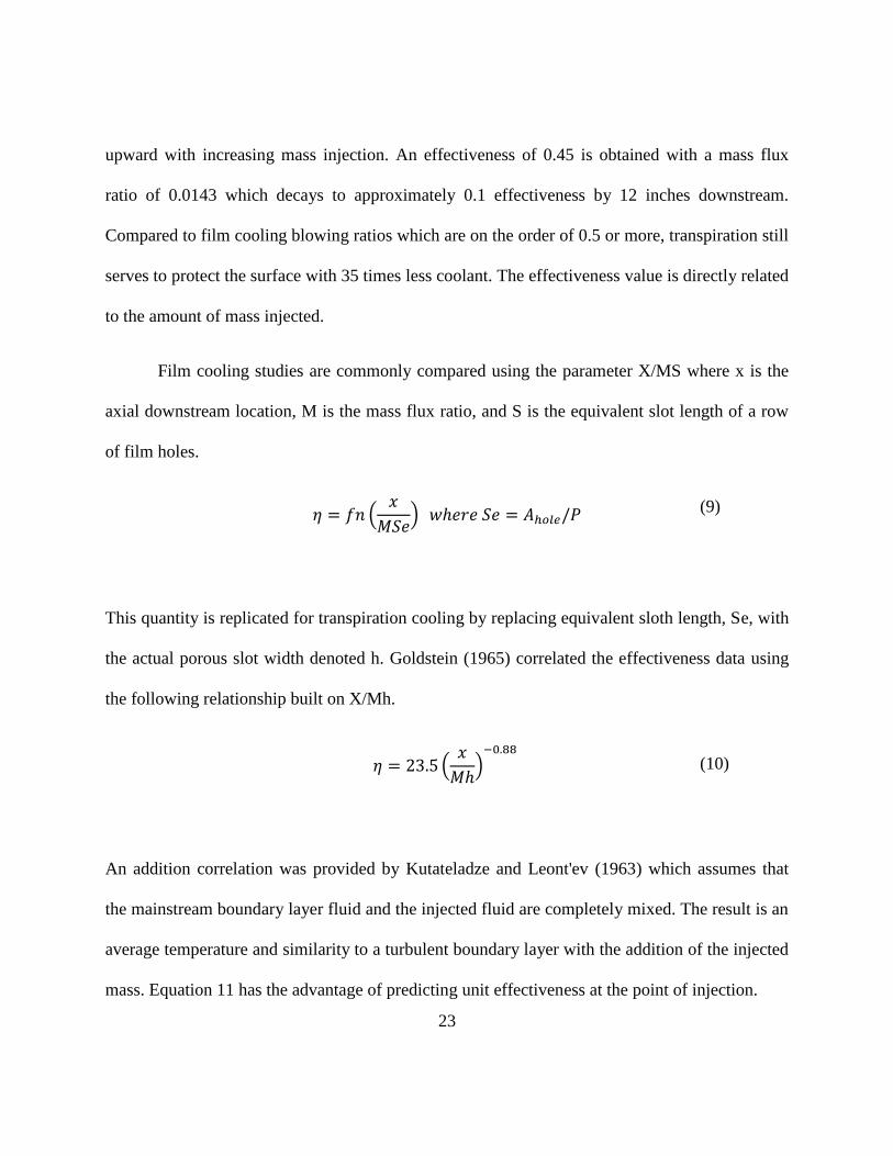
Film cooling studies are commonly compared using the parameter X/MS where x is the
axial downstream location, M is the mass flux ratio, and S is the equivalent slot length of a row
of film holes.
(
)
(9)
This quantity is replicated for transpiration cooling by replacing equivalent sloth length, Se, with
the actual porous slot width denoted h. Goldstein (1965) correlated the effectiveness data using
the following relationship built on X/Mh.
(
)
(10)
An addition correlation was provided by Kutateladze and Leont'ev (1963) which assumes that
the mainstream boundary layer fluid and the injected fluid are completely mixed. The result is an
average temperature and similarity to a turbulent boundary layer with the addition of the injected
mass. Equation 11 has the advantage of predicting unit effectiveness at the point of injection.

24
( (
)
)
(11)
Transpired turbulent boundary layers have been investigated in detail. Extensive research
has been provided by Kays (1972), Moretti and Kays (1965),and Georgiou and Louis (1985).
Morris and Foss (2003) provided a detailed characterization of the turbulent boundary layer after
a separation caused by a sharp discontinuation of the attached wall. Cal, Wang, and Castillo
(2005) performed an analysis of the effect of forced convection and external pressure gradients
on the transpired turbulent boundary layer. Lacking in these studies is experimental
characterization of the turbulent quantities as the flow leaves the permeable wall.
The rectangular free slot jet has been studied extensively, more than any noncircular
geometry. An extensive review can be found by Gutmark and Grinstein (1999). A transpiring
flow in the scenario of film cooling is essentially a rectangular slot jet with a porous blockage.
The turbulence generated in the near-field region of such a blocked jet is non-trivial; the
characterization of these turbulent quantities is necessary for accurate flow predictions by
Computational Fluid Dynamics (CFD).
Specifying accurate boundary conditions is essential when attempting to predict a
scenario in which there is flow exiting a permeable wall in CFD. A more accurate solution can

25
be obtained by using more accurate boundary conditions. The required conditions for the well-
known k-ε model are the turbulent kinetic energy (TKE) and turbulent dissipation rate (ε) values
at the boundary. Both k and ε can be estimated using the turbulence intensity and the turbulence
length scales. Hence, at bare minimum, estimations must be made of turbulence intensity and
turbulence length scales for two-equation models. The turbulence length scale is the physical
quantity describing the size of energy containing eddies in the turbulent flow and the turbulence
intensity is the RMS of the fluctuating component normalized by the local mean velocity (Fraser,
Pack, & Santavicca, 1986).

26
CHAPTER 3: NUMERICAL PREDICTIONS
First Order Analysis Domain
A domain is designed for the problem in order to compare all sources on an equal basis.
A hot gas path with cross section of 1m x 1m is being cooled on one wall over 0.25m. Film
geometry is installed at the leading edge of the domain. In the case of transpiration, 0.25m
following the end of the permeable section is investigated. In the case of discrete holes, the
0.25m domain begins at the trailing edge of the film row. Coupled scenarios of interest have a
transpiration section upstream of the film rows, in these cases the problem domain begins at the
trailing edge of the porous section and extends 0.25m downstream; the film source is always
contained within the problem domain.
Figure 9: Numerical Domain
Ma∞ , To,∞ , Po,∞, γ
MaC , To,C , Po,C, γ
0.25m
1m
1m
MaT , To,T , Po,T, γ
27
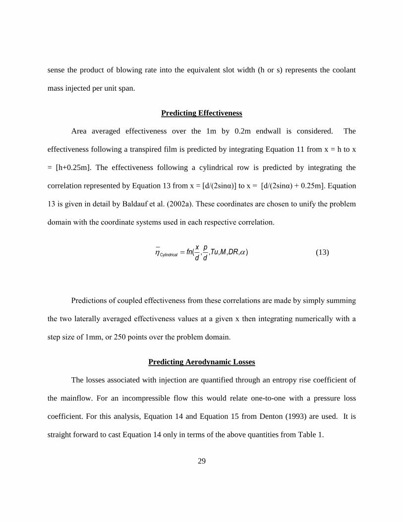
Physical quantities must be specified for the problem due to the some correlations
requiring absolute, rather than nondimensionalized quantities; moderate values are chosen
simply to give a physical feel for the problem rather than trying to predict against state-of-the-art
in which there is certainty of the validity of the relations used. The total temperature (1000 K)
and static pressure (20 atm) of the mainstream are prescribed and constant throughout the
analysis. The static temperatures are prescribed for the coolant sources. The transpired coolant
(600K) is a higher temperature than the film coolant (500K) because there will be more heat
addition to a transpired film than a discretely injected film as the coolant passes through the
permeable wall. At transpiration rate of M=0.1 and a transpiration slot width of 5mm, this
corresponds to a heat removal from the wall of 110kW. This value would change with
transpiration geometry and operating environment (e.g. volume and permeability of the porous
substrate) hence currently it is somewhat arbitrary. This added heat removal is one benefit of
transpiration. All other parameters governing the problem are shown in Table 1. The turbulence
intensity of the mainflow is kept low (1.5%) because only the correlation for cylindrical row
effectiveness has the ability to incorporate such information. The results from this analysis,
although for a generic problem domain, will be qualitatively the same as results from either low
speed testing or in an engine-like environment.

28
Table 1: Design Parameters
Parameter Mainstream, ∞ Cylindrical, C Transpiration, T
CP [J/kg-K] 1080 1080 1080
Ratio of specific heats - γ 1.4 1.4 1.4
Mach # - Ma 0.5 fn(M) fn(M)
Velocity [m/s] 309.3 fn(M) fn(M)
TO
[K] 1000 fn(M) fn(M)
T [K] 952 500 600
T∞/T , ρ/ρ∞ - 1.90 1.59
PO
[atm.] 23.7 fn(M) fn(M)
P [atm.] 20 20 20
PO/PO, ∞ - fn(M) fn(M)
Turb. Intensity [%] 1.5 - -
Predicting Mass Flow
After normalizing the coolant mass flow by the mass flow of the mainstream for the
given problem, the expression for mass flow ratio is given by Equation 12. The coolant spent
from a coupled source is the summation of both transpiration and discrete coolant mass flow
ratios.
𝐶𝑌𝐿𝑠 𝑁
(12)
Physically Equation 12 represents the coolant mass flow divided by the freestream mass
flow because the mainflow has a unit area and the transpiration is of unit span. In a general
29
sense the product of blowing rate into the equivalent slot width (h or s) represents the coolant
mass injected per unit span.
Predicting Effectiveness
Area averaged effectiveness over the 1m by 0.2m endwall is considered. The
effectiveness following a transpired film is predicted by integrating Equation 11 from x = h to x
= [h+0.25m]. The effectiveness following a cylindrical row is predicted by integrating the
correlation represented by Equation 13 from x = [d/(2sinα)] to x = [d/(2sinα) + 0.25m]. Equation
13 is given in detail by Baldauf et al. (2002a). These coordinates are chosen to unify the problem
domain with the coordinate systems used in each respective correlation.
( , , , , , )Cylindrical
x pfn Tu M DR
d d (13)
Predictions of coupled effectiveness from these correlations are made by simply summing
the two laterally averaged effectiveness values at a given x then integrating numerically with a
step size of 1mm, or 250 points over the problem domain.
Predicting Aerodynamic Losses
The losses associated with injection are quantified through an entropy rise coefficient of
the mainflow. For an incompressible flow this would relate one-to-one with a pressure loss
coefficient. For this analysis, Equation 14 and Equation 15 from Denton (1993) are used. It is
straight forward to cast Equation 14 only in terms of the above quantities from Table 1.

30
_
, ,2 2
,
_
cos( )11 1 1
2
Velocity Component
O C OC CP
O
Temperature Component
T Tm Vs C Ma Ma
m T V
(14)
,
212
O AVG
AVG
T s
V
(15)
One such relation is shown below in Equation 16 which relates the stagnation temperature of the
coolant, through an isentropic relation, to known quantities.
2
,
11
2 * *O Coolant Coolant
Coolant
MU
DRT TR T
(16)
Predicting Thermo-Mechanical Stresses
From the proposed method for computing averaged effectiveness, a maximum gradient in
effectiveness with respect to x/D or x/h can easily be computed by a first order finite difference
approach. The relation used for calculation of this gradient is shown in Equation 17.

31
2
( ) ( )x
D MAX
x x x
x
(17)
This quantity is of interest because thermal stresses are directly proportional to
temperature gradients on the surface. This approach for quantifying the thermal gradients is used
in order to provide a closed form method for calculating this quantity. Ideally, correlations, or
data, for local distributions of effectiveness could be computed for their gradients, and this
maximum would be chosen. These types of correlations are not nearly as common or general;
hence, for the sake of observing large ranges, this approach is taken. In the case of transpiration,
however, this is an adequate method for determining thermal gradients because there will be no
lateral gradients in effectiveness (assuming a very uniform permeable wall). In the case of
discrete holes, this method severely under-predicts the maximum gradient present, hence, the
maximum effectiveness gradient results must be interpreted cautiously.
The majority of the following graphs in this section are presented as follows; mass flow
ratio in the top left, average effectiveness over the endwall of the problem domain in the top
right, entropy rise coefficient broken up into its two components in the bottom left, and the
maximum gradient in laterally averaged effectiveness with respect to the streamwise coordinate
normalized by the injection geometry reference length (h in the case of transpiration, d in the
case of discrete holes.)
Transpiration cooling results for the quantities of interest are shown as a function of
blowing ratio for several transpiration section lengths in Figure 10. Equation 11 is used to predict

32
the average effectiveness following the permeable section in this instance. The benefits of
transpiration can be seen as an increase in blowing rate that causes a corresponding increase in
effectiveness. Due to the transpiration section being infinitely long spanwise, the main flow has
no path to the wall. Hence, the adiabatic film effectiveness will be unity, by definition,
immediately downstream of the porous section which contributes to the high levels of area
averaged effectiveness throughout the domain. The mass injected, MTRANh, contributes to the
rate of decay from this starting point. A small value of MTRANh implies a low thermal capacity
of the film resulting in quickly diminished effectiveness values.
Figure 10: Transpiration Analytical Results
Transpiration
M
En
tro
py
Ris
eC
oe
ffic
ien
t
0.05 0.1 0.15 0.2-0.04
-0.03
-0.02
-0.01
0
0.01
Temperature component
Velocity component
Increasing slot size
M
d(E
ta)/
d(x
/h)|
ma
x
0.05 0.1 0.15 0.210
-2
10-1
100
101
Increasing slot size
For a given mass flow and coolinglevel it is beneficial, from a thermal gradientstandpoint, to maximize blowing ratio whileminimizing slot size.
M
Ma
ss
Flo
wR
ati
o
0.05 0.1 0.15 0.20
0.00
1
0.00
2
0.00
3
0.00
4
0.00
5h=0.001 m
h=0.003 m
h=0.005 m
h=0.007 m
h=0.009 m
h=0.011 m
Increasing slot size
M
Av
era
ge
Eff
ec
tiv
en
es
s
0.05 0.1 0.15 0.20
0.05
0.1
0.15
0.2
Increasing slot size

33
When looking at the circled points on Figure 10 and comparing the effect of MTRANh, one
does not see a preference of blowing ratio to either large MTRAN or h. That is, the level of
downstream effectiveness following a transpiring section is not affected by whether the
transpired film jetted out through a short section, or was bled through a long section. The
gradient, however, is affected by the manner through which the coolant is injected. For the same
amount of mass injected, MTRANh, a short section operating at high blowing rates results in a
lower maximum thermal gradient than a long section operating at low blowing.
The cylindrical film cooling results are shown in Figure 11. Again, Equation 12,
Equation 14, and Equation 17 are used to calculate mass flow ratio, entropy rise coefficient, and
maximum thermal gradient, but in this case Equation 13 from Baldauf et al. (2002a) is used to
calculate average effectiveness. Unlike transpiration, discrete injection of coolant shows
diminishing returns when looking at effectiveness. All pitches, save for P/D=2, show that as the
blowing rate is increased from zero the average effectiveness downstream rises to a maximum,
after which, when the blowing rate is further increased until the extent of the range, MCYL=2.0,
the effectiveness drops. In the case of cylindrical holes, looking at the streamwise gradient is
misleading because the range of effectiveness values is from η=0-1, η=0 at mid span and η=1
downstream of a hole. This range then averages out to a value which changes slowly with axial
distance. In this situation the gradient in average effectiveness is presented for an analytical
perspective. The true gradient driving thermal stresses, however, in the case of discrete film
holes, is the gradient in the lateral, z-direction. Discrete holes are seen to be better than
transpiration in an aerodynamic sense when considering the entropy rise of the main flow due to

34
injection. As the transpiring rate is increased the aerodynamic penalty is increased, this is not the
case for discrete injection with an inclination angle of 30 degrees. For discrete injection, the
penalty rises slightly with blowing ratio until the momentum if the jet becomes comparable with
that of the main flow, in which case, the entropy rise coefficient begins to drop from its
maximum.
Figure 11: Discrete Hole Film Cooling Analytical Results
Cylindrical
M
En
tro
py
Ris
eC
oe
ffic
ien
t
0.5 1 1.5 2 2.5-0.04
-0.03
-0.02
-0.01
0
0.01
Temperature Component
Velocity Component
Increasing P/D
M
d(E
ta)/
d(x
/D)|
ma
x
0.5 1 1.5 2 2.510
-2
10-1
100
101
Misleadingly predicts a lower averagegradient for large P/D
M
Av
era
ge
Eff
ec
tiv
en
es
s
0.5 1 1.5 2 2.50
0.05
0.1
0.15
0.2
Large P/D are of most interest
M
Ma
ss
Flo
wR
ati
o
0.5 1 1.5 2 2.50
0.00
1
0.00
2
0.00
3
0.00
4
0.00
5
P/D=2
P/D=3
P/D=4
P/D=5
P/D=6
P/D=7
Increasing P/D

35
With the behaviors of each baseline source understood, a linear superposition of the two
is used in order to predict the behavior of a coupled source. Figure 12 (top) shows the effect of
offsetting the two individual sources from one another in a coupled scheme. The offset (O)
between the two is defined in this case as the distance between discrete hole center and
transpiration leading edge for this analysis. Shown at the bottom of Figure 12 are contours of
laterally averaged effectiveness in x-O space. The effect of moving the film row downstream
from at first being adjacent to the transpiration results in a slow decay from a maximum at
O/D=0 as the offset is increased. This analysis result in a prediction of maximum effectiveness
when the two geometries are adjacent to one another, which decreases as the cylindrical row is
moved downstream. The current method for coupling the two sources is insensitive to effects
resulting from the interaction of the two sources. The correctness of the simplified analysis must
be checked in a further study.

36
Figure 12: (Top) Offset Analysis, (Bottom) Effectiveness Contours
In Figure 13 the effect of each source’s blowing ratio is analyzed with constant
geometries of; h=5mm, D=7.5mm, O=0mm. From the figure it can be seen that the transpiration
blowing ratio shifts the results, this is because the assumptions used do not have any coupling
between equations, hence, only translations are seen through the coupled analysis. One key
feature to note is that the maximum streamwise gradient in effectiveness is solely governed by
the decay of the transpired film. There is no effect due to cylindrical blowing ratio.
0.25
0.2
0.3
0.35
0.4
0.45
0.5
0.2
0.15
0.15
Offset (m)
x(m
)
0 0.05 0.1 0.15 0.2
0.1
0.2
Offset (m)
Av
gE
ta
0 0.05 0.1 0.15 0.20.2
0.25
0.3
0.35
0.4

37
Figure 13: Effect of Blowing Ratio
The effect of changing the geometrical features of the two sources is shown in Figure 14
with constant blowing rates; MTRAN=0.05, MCYL=0.7. Again, it can be seen the transpiration
geometry only tends to shift the prediction versus a solo cylindrical geometry. The transpiration
is the major contributor to the value for maximum effectiveness gradient. From Figure 14, a
P/D=8 geometry with h/D=1.5 operating at the given blowing ratios, performs just as well as a
cylindrical row of P/D=2 at one third of the spent coolant and with an equal aerodynamic
penalty. Film rows alone at any spacing of P/D=3 or greater cannot obtain the level of cooling
resulting from this coupled scenario. From this analysis it seems possible that by coupling the
Coupled
Mcyl
En
tro
py
Ris
eC
oe
ffic
ien
t
0.5 1 1.5 2 2.5-0.04
-0.03
-0.02
-0.01
0
0.01
Increasing transpiration rate
Velocity Component
Temperature Component
Mcyl
d(E
ta)/
d(x
/D)|
ma
x
0.5 1 1.5 2 2.510
-2
10-1
100
101
Increasing transpiration rate
Maximum streamwise gradient completely a functionof the transpiration blowing rate for this film geometry
Mcyl
Ma
ss
Flo
wR
ati
o
0.5 1 1.5 2 2.50
0.00
1
0.00
2
0.00
3
0.00
4
0.00
5Mtran=0.01
Mtran=0.03
Mtran=0.05
Mtran=0.07
Mtran=0.09
Increasing transpiration rate
Mcyl
Av
era
ge
Eff
ec
tiv
en
es
s
0.5 1 1.5 2 2.50
0.05
0.1
0.15
0.2
Increasing transpiration rate
Additive approach results in a shift in resultsdue to coupling, no cross-coupling effectsare predicted with current methodology

38
two sources one can have the best of both worlds, the effectiveness of a transpiration source with
the losses of a discrete row.
Figure 14: Effect of P/D and h/D
Coupled
P/D
En
tro
py
Ris
eC
oe
ffic
ien
t
2 3 4 5 6 7 8-0.04
-0.03
-0.02
-0.01
0
0.01
Temperature component
Velocity component
Increasing slot size
P/D
d(E
ta)/
d(x
/D)|
ma
x
2 3 4 5 6 7 810
-2
10-1
100
101
Increasing slot size
P/D
Av
era
ge
Eff
ec
tiv
en
es
s2 3 4 5 6 7 8
0
0.05
0.1
0.15
0.2
Increasing slot size
P/D
Ma
ss
Flo
wR
ati
o
2 3 4 5 6 7 80
0.00
1
0.00
2
0.00
3
0.00
4
0.00
5h/D=0.1333
h/D=0.4
h/D=0.6666
h/D=0.9333
h/D=1.2
h/D=1.4666
Increasing slot size

39
Coupled Geometries
Both elements of the coupled geometry have particular roles that need to be filled.
The role of discrete holes
Mitigate losses
Provide strategic thermal mass
Loss mass flow few holes placed far apart due to a required minimum mass usage
The role of transpiration
High effectiveness
Uniform effectiveness
Low mass flow
Goals of a coupled geometry:
Low aerodynamic impact
Uniform effectiveness low thermo-mechanical impact
Low coolant mass flow rate
From the previous analysis and requirements, a test matrix is chosen. It will be the goal of
the discrete hole injection to use very little mass. The mass that is used will aide in thermal
capacity of the resulting film while mitigating aerodynamic penalties. From this perspective a
large pitch is required at as low an inclination angle as possible. This approach has led to the
geometry outlined in Table 2.
Table 2: Cylindrical Hole Parameters
Baseline - Cylindrical
Inclination angle, α (deg) 30
Compound angle, β (deg) 0
Hole diameter, D (mm) 7.5
Lateral pitch, P/D 3,6,9
Hole length, L/D 5

40
The transpiration source will provide most of the film to the boundary layer. However, it
must not use an unnecessary amount of coolant. In order to balance the competing effects of
mass flow consumption and thermal gradient, h/d=2/3 is chosen based on Figure 14. All
parameters dictating the transpiration source are outlined in Table 3.
Table 3: Transpiration Parameters
Baseline - Transpiration
Inclination angle, α (deg) 90
Injection length, h (mm) 5
Injection thickness, t (mm) 6
Permeable wall Aluminum foam
Porosity, ε (%) 50
RMS pore diameter, δ (mm) 0.1
Two coupled geometries are constructed from the above baseline configurations. First,
the above geometries are combined with an offset of one diameter, transpiration upstream, which
results in the Coupled A geometry. The effect of transpiration location relative to the row will be
seen through Coupled B which places the transpiration one diameter downstream of the
cylindrical row. The coupled geometries are described below in Table 4.

41
Table 4: Coupled Geometries
Coupled Geometry A (Baseline) B (Displaced)
Cylindrical Holes
Inclination angle, α (deg) 30 30
Compound angle, β (deg) 0 0
Hole diameter, D (mm) 7.5 7.5
Hole length, L/D 5 5
Transpiration
Inclination angle, α (deg) 90 90
Injection length, h (mm) 5 5
Injection thickness, t/h 1.2 1.2
Offset, O/D 1 -1
Finalized Geometries
Baseline geometries are shown in Figure 15. Portion (a) shows the standard cylindrical
holes with 30º inclination angle and a spanwise hole spacing (P/D) of three diameters and a
maximum of 13 holes for the closely spaced geometry. Part (b) shows the transpiration setup; a
slot is left open for a transpiring wall. In order to create the permeable section needed, ERG
Aerospace created an aluminum foam coupon which is then crushed to a denser, more realistic
porosity to provide realistic pressure drops. The material is aluminum 6101-T6 of ε=0.93 and 40
ppi crushed to a nominal value ε=0.5; only one half of its volume is comprised of aluminum.
42
Actual samples received vary only a small percentage from the nominal value. The crushing
process was done in a way as to retain a more isotropic pore after crushing.
Figure 15: Baseline Geometries. (a) Cylindrical Row, (b) Transpiration Section
The coupled geometries are shown in Figure 16. Part (a) features a row of 13 film holes
with a spacing of three diameters followed by the transpiration slot having an aspect ratio of 61;
leading to the assumption of it being infinite in the spanwise direction. The streamwise
dimension, h, was five millimeters. The second geometry, shown in (b), has the transpiration slot
upstream of the film holes. The spacing between the slot and the row of jets is 1.5 times the
thickness of the transpiration slot. The hole pattern and dimensions are constant for both Coupled
A and B.

43
Figure 16: Coupled Geometries. (a) Transpiration Upstream, (b) Transpiration Downstream, dimensions in mm.

44
CHAPTER 4: EXPERIMENTAL SETUP
Wind Tunnel
The main flow is generated by a 6kW Ziehl-Abegg fan capable of 1.6kPa and 7m3/s. The
cross flow duct is 110D wide by 20D tall. The duct is tall enough to ensure no influence on the
behavior of the jet due to the opposite wall. Access is also provided for various probe
measurements so that the boundary layer growth and aerodynamic losses can be assessed using
boundary layer and hot wire probes. The bottom acrylic view plate which serves as the majority
of the bottom wall of the cross flow duct is removable. Separate acrylic windows were
fabricated, one for probe access, and one for complete unobstructed optical access. The
experimental apparatus diagram is shown in Figure 17.
Figure 17: Experimental Apparatus
45
The flow is guided into the cross flow duct by a 3:1 bell mouth nozzle converging to the
test section dimensions. The flow is then conditioned by 2 honeycombs (DH=0.5”, L/D=6) and a
mesh screen. Following the flow conditioning section is a sandpaper trip to ensure a fully
turbulent boundary layer. The test section is 10cm downstream of this trip. At the first row of
discrete holes, the hydrodynamic boundary layer based on 95% of the freestream velocity is
measured to be 10mm. The freestream velocity reaches 26.5m/s over the entire test section. The
test section is assumed to be a zero pressure gradient duct; this is confirmed experimentally to be
valid with a pressure gradient of -15Pa/m over the test section. Turbulence intensity of the wind
tunnel is considered low, 0.7%, measured by constant temperature anemometer. The turbulent
length scale, calculated by the integration of the autocorrelation coefficient until the first zero
crossing, is 3.1cm.
An external air compressor is used to feed the coolant flow. Mass flow is metered
through a calibrated venturi flow meter. The flow is directed through an inline heater into an
insulated steel plenum. The plenum to coolant area ratio is sufficiently large (>100) to justify the
assumption that the coolant mass flow is equally divided between the film holes. The film hole
mass flow rates are calibrated using a calculated discharge coefficient and the static pressure of
the plenum. Therefore the mass flow solely through the film holes can be determined using the
static pressure of the plenum. The difference between total mass flow and calculated film mass
flow is equal to the transpiration mass flow rate. The coupled flow mass flow rate is completely
determined using the venturi flow meter and the static pressure. The error sensitivity to leaks is
high; therefore the consistency of discharge coefficients was verified (Natsui, Johnson, Torrance,
Ricklick, & Kapat, 2011). Great care is taken to ensure that the possibility of leaks is minimized.

46
The miniscule amount of coolant sent through the porous section compared to the film mass flow
ensures that the transpiring flow has no effect on the flow through the cylindrical holes.
Hot-wire Anemometry
In order to characterize the boundary conditions of the transpiring flow, a separate
experimental setup was created. The slot jet consists of a 17.2 mm thick acrylic coupon with a
slot milled for the porous blockage. The slot length and width, denoted l and h, are 305 mm and
5 mm respectively. The aspect ratio of this rectangular slot, given by l/h, is 61. The flow
originates from a compressed air line supplied by a 0.1 kg/s air compressor. The flow is metered
by a venturi flow meter before the inlet of the plenum. The plenum measures 100x20 slot widths
by 40 slot widths tall. Inside the plenum, the flow is redirected radially by a splashbox.
Downstream flow conditioning consists of a series of fine mesh screens. The slot jet coupon
attaches to the end of the plenum with gasket material and a series of clamps. The plenum and jet
coupon are detailed in Figure 18.
Figure 18: (a) Plenum Setup, (b) Transpiration Coupon
In order to create the permeable section needed, ERG Aerospace created an aluminum
foam coupon which is then crushed to a more realistic porosity to provide realistic pressure
drops. The material is aluminum 6101-T6 of ε=0.93 and 40ppi crushed to a nominal value ε=0.4,

47
0.5, and 0.6. Actual samples received vary only a small percentage from the nominal value, as
reported by the manufacturer. The crushing process is done in a way as to retain a more
isotropic pore after crushing. The porous insert measures 305mm by 5mm and 6.5mm in the
streamwise direction.
Table 5: Hot-Wire Test Parameters
The hot wire probe is located immediately following the test coupon. The hot wire is
allowed to traverse in the spanwise direction as well as the perpendicularly to the test coupon.
Hot wire measurements of turbulence are in error when using a wire with length the same order
as the length scale (Dryden, Shubauer, Moch, & Skramstad, 1937). The hot wire is chosen in
order to minimize the diameter of the wire and to achieve a length to diameter ratio of greater
Test Parameters
Jet Conditions
Reynolds Number, ReDe 7500
Reynolds Number, Reh 850
Darcy Velocity [m/s] 2.7
Permeable inserts
Porosity 0.379, 0.485, 0.616
Dimensions [mm] 5x305x6.5

48
than 20. The model used is a TSI Model 1201 hot wire with a diameter of 50.8 μm and length of
1.02 mm. The hot wire is calibrated using a TSI model 1125 calibrator.
A TSI IFA-300 anemometer controls the hotwire probe and utilizes a high pass filter at 1
Hz and a low pass filter at 50 kHz. Samples are taken at 100 kHz for 300k samples at each data
point. Measurements are digitized utilizing a National Instruments PXIe-6366 DAQ card using a
PXIe-1062Q chasis. The DAQ card features 8 channels and 16-bit resolution and is capable of 2
MS/s per channel. Traverses are made using a Velmex model #A2512P40-S2.5 combined with
model #A1509P40-S1.5, giving X-Z movement at 2.54 µm resolution. Data points are taken
laterally every 12.7 µm at 1, 2, and 3 slot widths vertically from the exit.
Turbulence Length Scale
The basis of characterizing turbulence depends on G. I. Taylor’s Frozen-Flow Turbulence
hypothesis. This hypothesis states that the larger integral scales provide the majority of the
advection energy compared to the turbulent circulation advection. This is only valid when the
smaller integral scales have sufficiently less power than the larger scales (Holm, 2005). The
significance of this hypothesis is that it allows an estimation of the spatial fluctuations of the
turbulent eddies from the temporal fluctuations at a single point. An extensive review of
different methods of calculating a turbulent length scale was performed by Barrett and
Hollingsworth (2001). Two length scales are taken from Barrett and the references used in
(Barrett & Hollingsworth, 2001). ΛI and ΛIII are calculated and denoted by L1 and L2
respectively.
49
The integral time scale is the integration of the autocorrelation coefficient function function
given by Equation 18. A length scale can be found by multiplying the time scale by the mean
velocity, Equation 19. This length scale that uses the integration of the autocorrelation can be
seen as a measure of the longest significant correlation time between the velocities at two points
in the flow field (Hinze, 1975).
∫
(18)
∫
(19)
An alternate definition of the time scale is based on the Fourier energy spectrum; this is
preferred in order to avoid the errors inherent to numerically integrating the autocorrelation
function (Lewalle & Ashpis, 2004). This requires the use of the energy spectrum at zero
frequency. An approximation can be had by taking a well converged part of the Fourier
spectrum and extrapolating it to the lower frequencies. The Welch method is used to
approximate the Fourier spectrum, by dividing the record in many sub-records (typically >1000)
with 50% overlap, the power spectrum is estimated on each sub-record by applying a Hamming
window (Welch, 1967). A discrete Fourier transform is used to calculate a modified periodogram
for each section and then averaged.
50
(20)
(21)
A length scale can be calculated from Equation 20 using Equation 21 (Barrett & Hollingsworth,
2001). The extrapolation relies heavily on low frequency information.
Transpiration Numerical Study
The experimental domain is modeled using GridPro and simplified to reduce the
computational requirements. The slot is modeled and shortened within the computational
domain, with symmetry planes along the bounding walls. The domain begins 15 slot widths
upstream of the leading edge and continues to 45 slot widths downstream. The crossflow is
modeled to five diameters above the surface in following with Johnson, Nguyen, Ho, and Kapat
(2010). A transpiring segment is modeled using a constant velocity inlet.

51
Figure 19: Computational Domain
The lower crossflow surface is treated as a no-slip adiabatic wall. The two planes normal to the
lateral direction were given symmetry conditions. In this way, the model mathematically
represents an infinite width of transpiration cooling. The freestream plane at five diameters
above the crossflow wall was also given symmetry conditions for reasons of computational
convenience rather than physical meaning. This is expected to have little effect on the film
cooling effectiveness results, which typically stay within two-diameters of the crossflow wall.
The analysis of Johnson et al. (2010) supports this expectation. A pressure-outlet condition
(prescribed uniform pressure with zero-gradient for other variables) is set at the outlet 45 slot
widths downstream of the hole. A uniform velocity-inlet is set at transpiring segment such that
the mass flow corresponds to a chosen blowing ratio. The temperature is set to 350 K (following
the experimental conditions). The inlet to the crossflow is also a velocity inlet, but here a
boundary layer profile is prescribed for the velocity. A power-law fit from an experimental
velocity profile was applied. The crossflow temperature is specified at 300K to imitate
experimental conditions and the turbulence quantities at the crossflow inlet are derived from
experimental measurements of turbulence intensity and length scale.

52
Crossflow turbulence intensity is taken to be 0.7% with a length scale of 0.01m, as
measured by hot wire anemometer. Transpiration turbulence intensity is taken to be the averaged
measured turbulence intensity of 2.296%. The length scale of the transpiration turbulence is
varied over the calculated values for the three porous inserts tested. An additional test is run
using a length scale based off the hydraulic diameter of the slot. Length scales are varied in order
to simulate changing the porosity of the wall insert without explicitly modeling the porous wall.
The realizable k-ε turbulence model was used with enhanced wall treatment.
The algebraic multi-grid (AMG) solver in Fluent was used to solve the coupled
equations. The SIMPLE technique was used for pressure-velocity coupling. The solution was
solved in steady-state, with under-relaxation factors acting to control convergence in the same
way time step would for a transient solution.
Grid Independence
This grid study consisted of a total of six grids, representing stages of systematic
refinement. The coarsest grid was just over 100,000 cells while the finest grid exceeded 2
million cells. Figure 20 shows the grid convergence index (GCI) for 15 temperature points and 5
velocity points in the flow. The most uncertain points are the temperature points on the surface
near the injection point. Once those safely converged under 10% uncertainty, the other points,
especially those away from the wall, converged to much lower GCI. It was seen in the GCI
method analysis that the complex geometry of the mesh did not lend to ideally-behaved
convergence with refinement for all monitors.

53
Figure 20: The converging GCI indices for 20 point monitors
The solution was started on the coarser grid and advanced for 100 iterations to achieve a
quality initial guess for the refined grid. The built-in geometry-based adaption in Fluent was then
utilized for embedded refinement in the area of interaction between the coolant and crossflow.
The refinement was bounded only in the y-direction, extending from the bottom wall to three slot
widths above the surface in the crossflow. The solution was then continued until convergence on
the finer grid. Convergence was judged by iterative convergence of monitors for the temperature
and velocity field as well as the normalized residuals of the governing equations. The criteria for
convergence of normalized residuals were as follows: below 1e-5 for continuity, below 1e-6 for
the momentum equation, below 1e-7 for the energy equation, and below 1e-5 for turbulence
quantities. Once the residuals fell below these marks and the temperatures and velocities no
longer changed to four decimals over a period of 100 iterations, the solution was treated as
converged. The results were then post-processed using the built-in capabilities of Fluent.
0
10
20
30
40
50
60
0.00E+00 5.00E+05 1.00E+06 1.50E+06 2.00E+06 2.50E+06
GC
I%
Number of Cells
54
Film Cooling Effectiveness
The film cooling effectiveness tests are run with a heated coolant, giving a density ratio
of approximately 0.85. An approximate 50 degree K temperature difference is maintained
between the coolant and the mainstream. Coolant temperature on average equaled 75°C (350K)
controlled by the inline heater while the freestream temperature was largely dictated room
temperature conditions (25°C, 300K). Three Type T (copper-constantan) thermocouples
measured the coolant temperature. Two are placed in the coolant plenum while one was inserted
into a film hole. The coolant temperature increased negligibly through the film hole. The
freestream temperature is taken as the recovery temperature measured from the test surface,
measured by Temperature Sensitive Paint (TSP) and verified by thermocouple mounted on the
surface. Additional thermocouples mounted in the freestream are used as a sanity check of
freestream temperature. The test coupon, a removable insert featuring the injection geometry, is
fitted in the test plate which forms the upper wall of the mainstream duct. Both features are
machined out of acrylic. The coupled geometry coupons include both discrete holes and a
rectangular slot. The porous aluminum insert is fitted and sealed into the rectangular slot. The
aluminum inserts were purchased from ERG Aerospace. The material is aluminum 6101-T6 of
ε=0.93 and 40 ppi crushed to a nominal value ε=0.5; only one half of its volume is comprised of
aluminum. Actual samples received vary only a small percentage from the nominal value. The
crushing process was done in a way as to retain a more isotropic pore after crushing.
Downstream of the injection coupon, a low thermal conductivity (0.029 W/m-K),
Rohacell® RIMA plate is fixed in the acrylic test plate to form an adiabatic wall. Rohacell is
closed cell foam of a composition that is able to resist the solvents in TSP. The Rohacell surface

55
facing the freestream flow is dry sanded to minimize grain structures and is coated with multiple
coats of TSP. The final coat of TSP is finished with high grit sand paper to ensure an even
surface finish. The painted Rohacell plate is flush mounted in the acrylic test plate with a
negligible transition between the injection coupon and the test surface.
Experimental Geometries
In addition to the baseline discrete hole, baseline transpiration, and the two coupled
geometries listed in Table 4, four multi-row configurations are tested. These arrays are denoted
by their discrete hole film geometrical parameter [α/β/(P/D)], or equivalent transpiration
parameter as seen in
Table 6. The film arrays are inclined 30 degrees and one of the geometries has a 45 degree
compound angle. These arrays were tested in the same wind tunnel experimental setup,
consisting of acrylic plates containing the flow features with a downstream rohacell recovery
region. Figure 21 gives a visual indication of the naming convention used; further details can be
found in Natsui, Torrance, Miller, Ricklick, and Kapat (2011). The first geometry [30/45/14]
corresponds to one used by Mayle and Camarata (1975) and serves as a validation case. It
consists of staggered holes with a streamwise non-dimensional spacing of 14 and a spanwise
spacing of 12.1. The Mayle geometry is also tested without compound angle ([30/0/14]) to study
the effect of compound angle on effectiveness. The geometry denoted [30/0/7] consists of two
period film cooling rows with the same amount of mass injected every four rows as the other
film geometries to ascertain the effectiveness of this configuration. A multi-row transpiration
array, [90/0/1], is compared with these discrete arrays, generally at much lower injection rates;

56
however, the high rate on the transpiration array consumes the same amount of coolant as the
low rates on the discrete arrays. One section of transpiration is used for every four rows of
discrete hole.
Table 6: Multi-Row Geometries
Multi-row Geometry
[αo/β
o/(P/D)]
[30/45/14] [30/0/14] [30/0/7] [90/0/1]
Source Type Cylindrical Hole Cylindrical Hole Cylindrical Hole Transpiration
Inclination angle, α (deg) 30 30 30 -
Compound angle, β (deg) 45 0 -
P/D 14 14 7 -
X/D 12.1 12.1 12.1 48.4
Streamwise Rows 12 12 6 3
Hole Diameter (mm) 2.5 2.5 2.5 -
Injection length, h (mm) - - - 5
Injection thickness, L/D or t/h 8 8 8 1.3
M (low, mid, high) 0.5,1.0,1.5 0.5,1.0,1.5 0.5,1.0,1.5 0.06, 0.12, 0.18

57
Figure 21: Test geometries, from top; [30/0/14], [30/45/14], [30/0/7], [90/0/1]

58
Temperature Sensitive Paint
Local, high resolution, temperature measurements are possible using temperature
sensitive paint. TSP requires only optical access to the surface that needs temperature
measurements; there is no disruption of the flow field. The active ingredient in TSP is
luminescent molecules immobilized in the polymer based paint. Illuminating the TSP painted
surface with 475nm wavelength light (blue light emitting diodes) causes photons to excite the
luminophores moving them to a higher energy state. In order to return to the ground energy state,
the luminophore may either emit luminescent radiation or drop energy levels by a process known
as thermal quenching. The different energy levels and photophysical processes of luminophores
are described by the Jablonski energy level diagram (Figure 22). As the temperature increases,
the quantum efficiency of luminescence in most of the molecules decreases because at elevated
temperatures the frequency of intermolecular collision increases. This increased frequency
creates a higher probably of deactivation by external conversion. This effect associated with
temperature is thermal quenching (Liu & Sullivan, 2005). Therefore the intensity of emission
from the illuminated TSP surface is inversely proportional to the temperature of the surface. This
correlation can be established through calibration. A more detailed explanation of the physics
behind TSP is given by Liu and Sullivan (2005).

59
Figure 22: Jablonski Energy-Level Diagram
For every test piece painted with TSP, an additional Rohacell coupon is painted. This
coupon is placed in a vacuum chamber along with an electrical heater. A calibration curve is
established by taking measurements at multiple temperatures. The calibration curves have proven
to be robust and vary little between batches of TSP. A sample calibration curve is shown in
Figure 23.

60
Figure 23: Calibration Curve
Images of the TSP surfaces are taken with a scientific grade CCD camera, a PCO 1600,
through a high pass filter. TSP emits at a longer wavelength (525nm) than it takes to excite it
(475nm). Therefore the high pass filter removes the excitation light. In order to calculate
temperatures from an intensity distribution, two images must be taken. One image is taken at
“cold” wind-off conditions with a measured temperature distribution and one image is taken at
“hot” wind-on conditions where the temperature distribution is unknown. The ratio of intensities
of these two images, along with the calibration curve allows for temperatures to be calculated.
To reduce noise, four images are taken each at hot and cold conditions and averaged. The TSP
was purchased in aerosol cans from ISSI.
The high resolution (1200x1600) images allow for pixel by pixel temperature calculation.
Due to slight image variations between the wind-off and wind-on images, the wind-on images
had to be shifted to line up with the wind-off image. Image processing is done using MATLAB
y = 0.6173x2 - 1.4392x + 1.0220 R² = 0.9995
0
0.1
0.2
0.3
0.4
0.5
0.6
0.7
0.8
0.9
0.3 0.4 0.5 0.6 0.7 0.8 0.9 1
Tem
pe
ratu
re R
atio
/10
0, θ
Intensity Ratio, I/Iref

61
scripts written for this purpose. A bi-linear interpolation scheme is used for shifting the wind-on
images. This allows for sub-pixel image shifting before the temperatures are calculated.
Film Cooling Effectiveness Data Reduction
The film cooling effectiveness, presented earlier in Equation 2, represented by η, is a
nondimensional temperature ratio. The driving potential behind an effectiveness measurement is
the temperature difference between injected coolant and mainstream flow. Since the injected
mass flow rate is considerably less than the mainstream flow, it is more convenient to heat the
coolant flow rather than heat the mainstream. The smaller mass flow requires less energy input to
reach a usable temperature delta of 50°C. At the low temperatures of the study, 300 to 350 K,
and only a 50°C delta in temperature, it is valid to assume constant property flow. With this
assumption and the assumption of negligible radiant energy input, the film cooling effectiveness
(dimensionless temperature difference) in the boundary layer is independent of having a hotter or
colder injection flow (Goldstein, 1971). Realistically however, the density ratio of a real turbine
blade film cooling scenario is on the order of 2.0, opposed to 0.85 of this study. In general,
higher blowing rates are required for optimal cooling at higher density ratios compared to lower
density ratios (Baldauf, Scheurlen, Schulz, & Wittig, 2002b). Data from Pedersen et al. (1977)
indicates that as the blowing ratio is increased, the effect of density ratio increases, except near
the downstream exit of the film hole. The effect of density ratio cannot be neglected for the study
of film cooling effectiveness meant for gas turbine blade scenarios. The lateral averaging of film
effectiveness is carried out for the interior seven film holes; the three outside film holes on each
side are not included in the averaging window. This is to reduce possible end wall effects on the
lateral average.

62
Experimental Uncertainty
Uncertainty calculations were performed in accordance with the method proposed by
Kline and McClintock (1953). Multiple measurement devices were used wherever possible, for
example multiple thermocouples for each temperature measurement and multiple static pressure
ports for pressure measurements. Averages were taken of the respective measurement devices
and used for the true measured value. The uncertainty tree for adiabatic film cooling
effectiveness is shown in Figure 24. The tree represents the measurands in the Kline and
McClintock method.
Figure 24: Effectiveness Uncertainty Tree
The ‘adiabatic wall’ temperature is the wall temperature as measured by temperature
sensitive paint. Therefore the uncertainty inherent in that measurement technique contributes
only to one term in the film cooling effectiveness. Contributions to uncertainty in the
temperature sensitive paint measurement technique include paint thickness (luminophore
concentration) or variations in chemical/physical properties of the paint, illumination uniformity,
63
photodetector noise, wavelength overlap between illumination source and optical filter, photo
degradation, and temperature hysteresis. Through the use of an intensity ratio to calculate
temperatures, the dependence on absorption intensity is removed. Furthermore the effects of
spatial non-uniformities of illumination, paint thickness, and luminophore concentration are
removed as well by taking the ratio of intensities. Uncertainty in the adiabatic wall temperature is
taken to be ±0.5°C at 95% confidence level.
Mainstream temperature and coolant temperature are measured with multiple T-type
thermocouples each. Coolant temperatures are taken in the plenum as well as inside film holes
when available (holes nearest to the lateral walls were chosen since these are not used in the
lateral averaging window). These thermocouples are un-calibrated and required the usage of
extension cables. Contributors to uncertainty include heat flow along thermocouple leads,
extension cables, position bias, and the uncertainty in the thermocouple reader. Accordingly at
95% confidence level the uncertainty in mainstream temperature is ±0.4°C and coolant
temperature is ±2.8°C. Total uncertainty in the effectiveness measurement as calculated by the
method detailed in Kline and McClintock (1953) is ±0.0204 at 95% confidence level. The largest
contributor to the effectiveness uncertainty is adiabatic wall temperature uncertainty with 48.8%
of the total uncertainty coming from the adiabatic wall temperature. The coolant temperature
uncertainty accounts for 31.2% of the total effectiveness uncertainty; the mainstream temperature
accounts for the remaining 20% of the total effectiveness uncertainty. For a typical effectiveness
value of 0.2 ± 0.0204, adiabatic wall temperature contributes ±0.01. Reducing uncertainty would
benefit greatest from a reduction in adiabatic wall temperature uncertainty, followed by coolant
temperature uncertainty. The uncertainty is least sensitive to mainstream temperature.

64
Uncertainty of the hot-wire anemometer measurements are calculated using the same
method. Contributors to uncertainty include calibrator uncertainty, linearization, analog-to-
digital resolution, probe positioning, temperature variations, ambient pressure variations, and
humidity variations. The largest source of error is due to the calibrator used (TSI Model 1125
calibrator) which contributes 2% of the total 4% uncertainty at 95% confidence level in hot-wire
velocity measurements. The uncertainty in turbulence intensity is also 4% of the calculated
value.
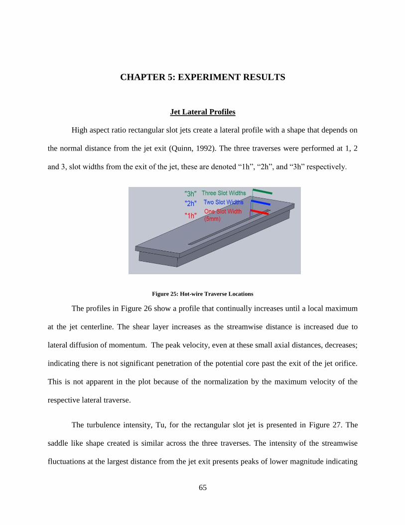
65
CHAPTER 5: EXPERIMENT RESULTS
Jet Lateral Profiles
High aspect ratio rectangular slot jets create a lateral profile with a shape that depends on
the normal distance from the jet exit (Quinn, 1992). The three traverses were performed at 1, 2
and 3, slot widths from the exit of the jet, these are denoted “1h”, “2h”, and “3h” respectively.
Figure 25: Hot-wire Traverse Locations
The profiles in Figure 26 show a profile that continually increases until a local maximum
at the jet centerline. The shear layer increases as the streamwise distance is increased due to
lateral diffusion of momentum. The peak velocity, even at these small axial distances, decreases;
indicating there is not significant penetration of the potential core past the exit of the jet orifice.
This is not apparent in the plot because of the normalization by the maximum velocity of the
respective lateral traverse.
The turbulence intensity, Tu, for the rectangular slot jet is presented in Figure 27. The
saddle like shape created is similar across the three traverses. The intensity of the streamwise
fluctuations at the largest distance from the jet exit presents peaks of lower magnitude indicating

66
most of the turbulence production occurs immediately after the jet exits the slot, where the shear
layer on either side is smallest. Approximately 60% of the peak turbulence intensity value, 15%,
is seen at the jet centerline for all locations. The location of maximum turbulence intensity does
not change; furthermore, the peak corresponds with the inflection point of the mean velocity.
Figure 26: Slot Jet Lateral Traverse Velocities
0
0.2
0.4
0.6
0.8
1
-1 -0.5 0 0.5 1
V/V
MA
X
x/δ
0.0 "1h"
0.0 "2h"
0.0 "3h"

67
Figure 27: Slot Jet Turbulence Intensities
The nominal 0.60 porosity insert creates a non-uniform velocity profile, shown in Figure
28. The profile taken at the first slot width location shows a velocity profile skewed to one side,
indicating the porous blockage acts to produce several smaller discrete jets. Further in the
streamwise direction, the distribution spreads as expected; however compared to a free jet, the
distribution peaks higher in the centerline with a more narrow spread. The individual jets allow
more diffusion of momentum to occur over a smaller distance based on slot width. The relevant
length-scale defining the growth of the shear layer is on the order of each individual pore size
0
0.04
0.08
0.12
0.16
-1 -0.5 0 0.5 1
Tu
x/δ
0.0 "1h"
0.0 "2h"
0.0 "3h"

68
rather than slot width due to the porous blockage. The distribution is still skewed to one side at
all downstream locations.
Figure 28: 0.6 Porosity Lateral Traverse Velocities
0
0.2
0.4
0.6
0.8
1
-1 -0.5 0 0.5 1
V/V
MA
X
x/δ
0.6 "1h"
0.6 "2h"
0.6 "3h"

69
Figure 29: 0.6 Porosity Turbulence Intensity
Compared to the free jet streamwise fluctuation distribution, Figure 27, the porous insert,
Figure 29, displays a backwards trend, the turbulence intensity magnitude increases as the
streamwise distance is increased from the jet exit. The porous blockage seems to be removing
energy from the turbulent fluctuations through the orifice. As the jet travels downstream, there is
a production of turbulent energy as the shear layers grow. The skewness is further illustrated
towards the right hand side. The three streamwise locations present similar asymmetric Tu
distributions.
The single slot width displacement lateral traverse of velocity for the nominal 0.5 porosity
porous piece shows a distribution that is largely asymmetric with a sharp decrease along the
0
0.01
0.02
0.03
0.04
0.05
0.06
-1 -0.5 0 0.5 1
Tu
x/δ
0.6 "1h"
0.6 "2h"
0.6 "3h"

70
centerline of the jet, seen in Figure 30. A local maximum is located on the far side of the porous
insert, indicating a concentration of open pores surrounded by a section of pores that are blocked.
The further streamwise traverses do not show this non-normal distribution; instead a bell curve
with distinct peak is presented. Only a slight indication of the other local maximum is seen,
indicating the jet spreading has evened the distribution nearly completely. Again, this spreading
occurs much more quickly than it would if the length scale dictating diffusion were the slot
width. The porous insert acts to reduce the length scale of the jet. The furthest stream wise
traverse presents a peak in turbulence intensity approximately 160% greater than the other local
maximum, shown in Figure 31. This is likely due to the large gradients in the mean profile
causing a large production of TKE in this region. The one slot width displacement traverse also
shows this increase in turbulence intensity magnitude on that side of the porous slot; however the
two slot width case does not.

71
Figure 30: 0.5 Porosity Lateral Traverse Velocities
0
0.2
0.4
0.6
0.8
1
-1 -0.5 0 0.5 1
V/V
MA
X
x/δ
0.5 "1h"
0.5 "2h"
0.5 "3h"

72
Figure 31: 0.5 Porosity Lateral Turbulence Intensities
The velocity profile from the 0.4 porosity porous insert most resembles the distribution given
by the free jet. The 40% porosity blockage also has the smallest, most closely packed pores. The
one slot width traverse displays the non-uniformity of the velocity profile by having three
distinct peaks composing the overall jet, two distinct peaks on either side slot center (x/δ=0) and
a slightly smaller peak near x/δ=-0.5, shown in Figure 32. As the distance from the porous
section increases, the jet spreads more and becomes more uniform. The distribution of open
pores in this lateral traverse is seemingly even.
0
0.04
0.08
0.12
0.16
-1 -0.5 0 0.5 1
Tu
x/δ
0.5 "1h"
0.5 "2h"
0.5 "3h"

73
The turbulence intensity distribution for the 40% porosity porous insert displays the same
saddle distribution as the other porous filled jets, with similar magnitude for the two slot width
displacement cases. There is not a large production of TKE rather the fluctuations are overall
maintained as the jet travels downstream with a slight increase on one side, the side
corresponding to more curvature of the mean profile. An asymmetric peak is seen on one side of
the jet that dissipates as the distance is increased, seen in Figure 33. The normalized streamwise
fluctuation has three peaks in the 1h traverse. This is due to there being two individual, smaller
jets, on either side of slot center. They quickly merge, as seen in the mean profile, and form the
typical saddle shaped distribution of Tu.
Figure 32: 0.4 Porosity Lateral Traverse Velocities
0
0.2
0.4
0.6
0.8
1
-1 -0.5 0 0.5 1
V/V
MA
X
x/δ
0.4 "1h"
0.4 "2h"
0.4 "3h"

74
Figure 33: 0.4 Porosity Lateral Turbulence Intensities
The trend at the centerline of the porous jets is a discrete minimum in turbulence intensity,
seen for each porous insert. The turbulence production is occurring in the shear layer. The 2%
turbulence intensity seen at this location is independent of porosity and is 300% lower than the
free jet centerline turbulence intensity. The porous inserts display differing levels of peak
turbulence intensity due to the different distribution of open and closed pores as well as overall
nominal pore diameter. The net effect is a decrease in centerline turbulence intensity similar to
putting mesh screens upstream of the flow.
An autocorrelation of the streamwise fluctuation is calculated for each at one slot width in the
streamwise direction at the centerline of the jet; the 0.4 porosity case is shown in Figure 34. The
0
0.02
0.04
0.06
0.08
0.1
-1 -0.5 0 0.5 1
Tu
x/δ
0.4 "1h"
0.4 "2h"
0.4 "3h"
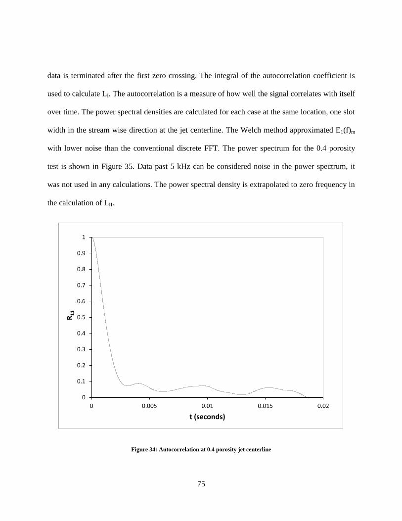
75
data is terminated after the first zero crossing. The integral of the autocorrelation coefficient is
used to calculate LI. The autocorrelation is a measure of how well the signal correlates with itself
over time. The power spectral densities are calculated for each case at the same location, one slot
width in the stream wise direction at the jet centerline. The Welch method approximated E1(f)m
with lower noise than the conventional discrete FFT. The power spectrum for the 0.4 porosity
test is shown in Figure 35. Data past 5 kHz can be considered noise in the power spectrum, it
was not used in any calculations. The power spectral density is extrapolated to zero frequency in
the calculation of LII.
Figure 34: Autocorrelation at 0.4 porosity jet centerline
0
0.1
0.2
0.3
0.4
0.5
0.6
0.7
0.8
0.9
1
0 0.005 0.01 0.015 0.02
R1
1
t (seconds)
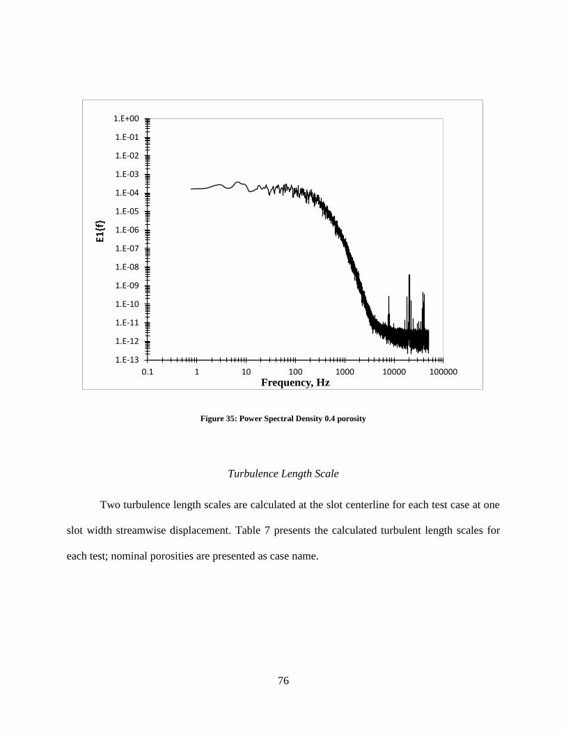
76
Figure 35: Power Spectral Density 0.4 porosity
Turbulence Length Scale
Two turbulence length scales are calculated at the slot centerline for each test case at one
slot width streamwise displacement. Table 7 presents the calculated turbulent length scales for
each test; nominal porosities are presented as case name.
1.E-13
1.E-12
1.E-11
1.E-10
1.E-09
1.E-08
1.E-07
1.E-06
1.E-05
1.E-04
1.E-03
1.E-02
1.E-01
1.E+00
0.1 1 10 100 1000 10000 100000
E1{f
}
Frequency, Hz
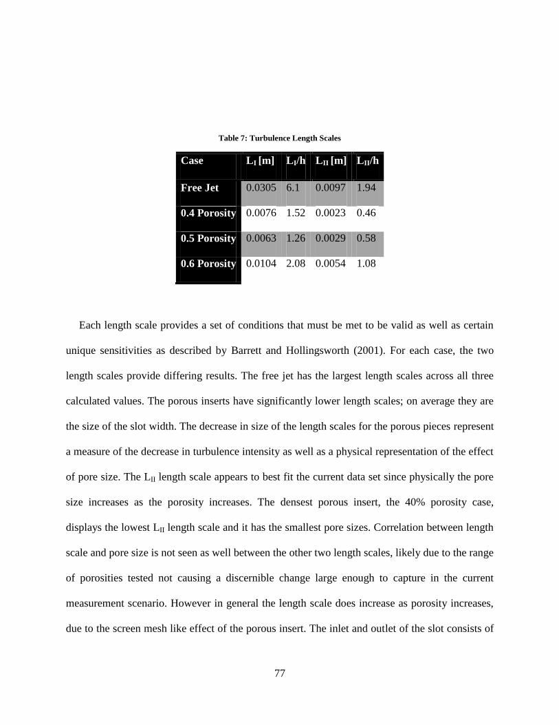
77
Table 7: Turbulence Length Scales
Case LI [m] LI/h LII [m] LII/h
Free Jet 0.0305 6.1 0.0097 1.94
0.4 Porosity 0.0076 1.52 0.0023 0.46
0.5 Porosity 0.0063 1.26 0.0029 0.58
0.6 Porosity 0.0104 2.08 0.0054 1.08
Each length scale provides a set of conditions that must be met to be valid as well as certain
unique sensitivities as described by Barrett and Hollingsworth (2001). For each case, the two
length scales provide differing results. The free jet has the largest length scales across all three
calculated values. The porous inserts have significantly lower length scales; on average they are
the size of the slot width. The decrease in size of the length scales for the porous pieces represent
a measure of the decrease in turbulence intensity as well as a physical representation of the effect
of pore size. The LII length scale appears to best fit the current data set since physically the pore
size increases as the porosity increases. The densest porous insert, the 40% porosity case,
displays the lowest LII length scale and it has the smallest pore sizes. Correlation between length
scale and pore size is not seen as well between the other two length scales, likely due to the range
of porosities tested not causing a discernible change large enough to capture in the current
measurement scenario. However in general the length scale does increase as porosity increases,
due to the screen mesh like effect of the porous insert. The inlet and outlet of the slot consists of

78
sharp edges, forcing the flow to enter aggressively, causing a large amount of TKE production,
and exit with enhanced levels of turbulence. The result is large length scales for the free jet case
compared to the porous cases.
Transpiration Numerical Results
A total of four CFD cases were run using various turbulence length scales for the
transpiring flow. LII was chosen for the length scale due to the purely increasing trend seen with
increasing porosity. Cases 1 through 3 correspond to porosities of 0.4 through 0.6 respectively.
Case 4 is unique in that it does not represent the free jet, but instead the turbulence length scale
was chosen to be the hydraulic diameter of the slot, a common choice of length scale. However
due to the similarity in length scale between the free jet and hydraulic diameter, the outcomes
will be identical. Table 8 shows the relevant boundary conditions.
Table 8: CFD Case Description
Case # TI [%] Blowing Ratio LII [m] LII/h
Case 1 2.296 0.100 0.0023 0.46
Case 2 2.296 0.100 0.0029 0.58
Case 3 2.296 0.100 0.0054 1.08
Case 4 2.296 0.100 0.0098 1.96
Blowing ratio and turbulence intensity were held constant between the four cases, leaving
the only changing parameter the turbulence length scale. The blowing ratio was chosen such that
it directly compared with one of the experimental test cases. During post processing, laterally

79
averaged film cooling effectiveness is calculated using planes of finite thicknesses at discrete
points downstream of the slot in the domain. Laterally averaged film cooling effectiveness for
the four cases is shown in Figure 36.
Figure 36: Transpiration CFD Laterally Averaged Effectiveness
The difference seen between the four cases is very slight. Figure 37 shows the difference
between each case and Case 1. The largest difference is seen near the slot exit with a different
behavior exhibited as the length scale increases. The effectiveness tends to decrease with
increasing turbulence length scale albeit only very slightly. Case 4 shows the largest difference
from Case 1 however that difference is very small. The current problem is not sensitive to
0
0.2
0.4
0.6
0.8
1
0 10 20 30 40
Late
rally
Ave
rage
d F
ilm E
ffec
tive
nes
s
X/h
Case1
Case2
Case3
Case4

80
turbulence length scale variation due to the low turbulence intensity. This parameter is not
sufficient to model the intended change in porosity of the porous wall.
Figure 37: Difference in Effectiveness from Case1
Experimental Validation
In order to validate the film cooling effectiveness measurements taken from the current
setup, validation runs were performed. Both the discrete hole and transpiration geometries were
run independently using coupons with only the respective feature.
-0.01
-0.006
-0.002
0.002
0.006
0.01
0 10 20 30 40
Del
ta f
rom
Cas
e1 E
ffec
tive
nes
s
X/h
Delta Case1 Delta Case2
Delta Case3 Delta Case4
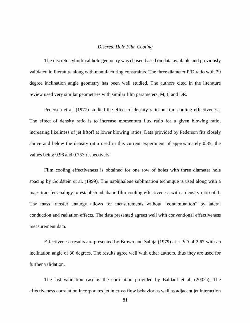
81
Discrete Hole Film Cooling
The discrete cylindrical hole geometry was chosen based on data available and previously
validated in literature along with manufacturing constraints. The three diameter P/D ratio with 30
degree inclination angle geometry has been well studied. The authors cited in the literature
review used very similar geometries with similar film parameters, M, I, and DR.
Pedersen et al. (1977) studied the effect of density ratio on film cooling effectiveness.
The effect of density ratio is to increase momentum flux ratio for a given blowing ratio,
increasing likeliness of jet liftoff at lower blowing ratios. Data provided by Pederson fits closely
above and below the density ratio used in this current experiment of approximately 0.85; the
values being 0.96 and 0.753 respectively.
Film cooling effectiveness is obtained for one row of holes with three diameter hole
spacing by Goldstein et al. (1999). The naphthalene sublimation technique is used along with a
mass transfer analogy to establish adiabatic film cooling effectiveness with a density ratio of 1.
The mass transfer analogy allows for measurements without “contamination” by lateral
conduction and radiation effects. The data presented agrees well with conventional effectiveness
measurement data.
Effectiveness results are presented by Brown and Saluja (1979) at a P/D of 2.67 with an
inclination angle of 30 degrees. The results agree well with other authors, thus they are used for
further validation.
The last validation case is the correlation provided by Baldauf et al. (2002a). The
effectiveness correlation incorporates jet in cross flow behavior as well as adjacent jet interaction

82
at engine-like conditions. This correlation was reconstructed utilizing values realized from the
current experimental setup.
Table 9: Validation Cases
P/D Inclination Angle
(degrees)
Density
Ratio Blowing Ratio
Current Study 3 30 0.85 0.4, 0.5, 0.8, 1.0, 1.2,
2.0
Pedersen et al. (1977) 3 35 0.75, 0.95 0.5, 1.0 2.0
Goldstein et al. (1999) 3 35 1.0 0.5, 1.0 2.0
Goldstein (1969) 3 35 <1.0 0.5, 1.0 2.0
Brown and Saluja
(1979) 2.67 30 1.1 0.5, 1.0
Baldauf et al. (2002a) 3 35 0.85 0.4, 0.5, 0.8, 1.0, 1.2
2.0
The baseline cylindrical case was run at blowing ratios of 0.4, 0.5, 0.8, 1.0, 1.2, and 2.0.
Experimental data from literature was found with blowing ratios of 0.5, 1.0 and 2.0. Therefore
those three blowing ratios were run for strictly validation purposes. Data was averaged
perpendicular to the stream wise direction (laterally) to provide a span averaged film cooling
effectiveness. The span averaged effectiveness for a blowing ratio of 0.5 can be seen in Figure
38.

83
Figure 38: Laterally average effectiveness M=0.5
At this density ratio of 0.83 and momentum ratio of 0.34, the jets stay attached to the surface
and decays linearly. The data agrees with Goldstein (1999) and Pederson (1977); the slower
decay could be due to the shallower angle of injection, 30 degrees, versus the 35 degree angle
used by Goldstein and Pederson. The shallower angle allows for greater stream wise momentum
which allows for less mixing with the main stream. The Baldauf correlation greatly over predicts
the span averaged effectiveness until nearly 30 diameters downstream of the film holes. This is
due to the correlation being generated from data tested at engine-like conditions, with engine-like
density ratios. The density ratios intended are greater than unity. The result is operating the
correlation out of the range in which it is valid. The data from Brown (1978) matches the
0
0.05
0.1
0.15
0.2
0.25
0.3
0 10 20 30 40 50
Late
rally
Ave
rage
d F
ilm E
ffec
tive
nes
s
X/D
M=0.53, DR=0.83, I=0.34
M=0.515, DR=0.753 -Pederson (1977)
M=0.515, M=0.96 - Pederson(1977)
M=0.5 - Goldstein (1999)
P/D=3, M=0.5, DR=0.9,I=0.278 (Baldauf Correlation)
M=0.5, DR=1.1 - Brown(1978)
M=0.5 - Goldstein et al.(1969)

84
measured data the best, due to the 30 degree inclination angle, however no data further than 15
diameters downstream is provided. Additional 35 degree inclination angle data is taken from
Goldstein (1969), which agrees well with the other 35 degree inclination data. “Coverage” is
frequently used in film cooling to refer to the ratio of open area at a row of film cooling holes to
the total are being cooled. For unshaped cylindrical holes, the coverage is simply the inverse of
the hole-to-hole spacing (also called pitch), P/D. The physical limit for laterally averaged film
cooling effectiveness immediately downstream of the first row is equal to the coverage, because
η ≤ 1 immediately downstream of the open area of the holes and η = 0 elsewhere. However
due to noise just downstream of injection, this trend is not seen in the experimental data.

85
Figure 39: Laterally Averaged Film Effectiveness at M=1.0
Span averaged effectiveness values for the blowing ratio of 1.0 are shown in Figure 39.
At this blowing ratio, distinct jet lift-off is present, which is not present in all of the data from
literature due to the differences in density ratio and subsequently momentum ratio. The Baldauf
correlation greatly over predicts effectiveness for the first 45 diameters downstream of the film
holes. The correlation must be assuming that the jet does not lift off at this blowing ratio and
stays completely attached. The data from Brown and Saluja (1979) agrees with the Baldauf
correlation for the limited data points provided. The larger density ratio used by Brown allows
the jet to stay attached and build greater effectiveness right after the film holes. The increase in
0
0.05
0.1
0.15
0.2
0.25
0.3
0 10 20 30 40 50
Late
rally
Ave
rage
d F
ilm E
ffec
tive
nes
s
X/D
M=1.05, DR=0.82, I=1.34
M=1.05, DR=0.743 - Pederson(1977)
M=1.05, M=0.953 - Pederson(1977)
M=1.0 - Goldstein (1999)
P/D=3, M=1.0, DR=0.9, I=1.11(Baldauf Correlation)
M=1.0, DR=1.1 - Brown(1978)
M=1.0 - Goldstein et al.(1969)

86
effectiveness approximately 25 diameters downstream may be due to an increase in turbulent
mixing between the coolant jet and main stream flow (Goldstein et al., 1999). The differences
between literature and the current measurements are explainable by the differences in inclination
angle and coolant properties (density ratio and momentum ratio).
Figure 40: Laterally Averaged Film Effectiveness at M=2.0
Further increasing the blowing ratio to 2.0 results in significant jet lift-off, causing a
period of very low effectiveness until the jet reattaches approximately 10 diameters downstream
of the film holes, shown in Figure 40. The increase in effectiveness after the jet reattaches is
0
0.05
0.1
0.15
0.2
0.25
0.3
0 10 20 30 40 50
Late
rally
Ave
rage
d F
ilm E
ffec
tive
nes
s
X/D
M=2.05, DR=0.87, I=4.83
M=1.96, DR=0.963 -Pederson (1977)
M=1.96, DR=0.742 -Pederson (1977)
M=2.0 - Goldstein (1999)
P/D=3, M=2.0, DR=0.9,I=4.44 (Baldauf Correlation)
M=2.0 - Goldstein et al.(1969)

87
significant; the jet spreading and subsequent strong turbulent mixing occurs further upstream
than the blowing ratio of 1.0 case (Goldstein et al., 1999). The Goldstein et al. (1999) data
agrees very well with the current study. The initially low effectiveness points towards a larger
magnitude of jet lift-off due to the steeper injection angle with a reattachment that agrees with
the current study. The Baldauf correlation under predicts the effectiveness, possibly due to using
a low density ratio on a correlation created using high density ratio data. The resulting effect
would be decreased lateral spreading due to the low density ratio, while expecting a large amount
of spreading due to correlating from high density ratio data (Sinha et al., 1991).
Figure 41: Laterally Averaged Film Effectiveness at M=0.4
0
0.05
0.1
0.15
0.2
0.25
0.3
0 10 20 30 40 50
Late
rally
Ave
rage
d F
ilm E
ffec
tive
nes
s
X/D
M=0.41, DR=0.85, I=0.20
P/D=3, M=0.4, DR=0.9, I=0.178(Baldauf)

88
Due to the lack of literature data at the blowing ratios of 0.4, 0.8 and 1.2, those are only
plotted against the Baldauf correlation for comparison. Due to the lower density ratio used in the
Baldauf correlation, the laterally averaged effectiveness reaches a high effectiveness peak at the
low blowing ratio of 0.4 (Baldauf et al., 2002a). The high peak is due to jet spreading at the exit
of the film hole, followed by a decay caused by the coolant being diluted by the mainstream
flow. The downstream effectiveness agrees very well past 30 diameters.
Figure 42: Laterally Averaged Film Effectiveness at M=0.8
0
0.05
0.1
0.15
0.2
0.25
0.3
0 10 20 30 40 50
Late
rally
Ave
rage
d F
ilm E
ffec
tive
nes
s
X/D
M=0.79, DR=0.82, I=0.76
P/D=3, M=0.8, DR=0.9, I=0.711(Baldauf)

89
The blowing ratio of 0.8 can be considered a critical value where the jet is very close to
the momentum ratio required to lift from the surface. The result is a flat profile which can be
considered to decay very slightly (within experimental uncertainty. Compared to the blowing
ratio 1.0 data, it can be seen that very near the hole exit a very slight, partial jet detachment. The
effectiveness slightly increases from the jet reattaching, but since the jet never fully detached,
only small amounts mainstream flow are entrained underneath the jet. The effectiveness curve
shape can be seen in data by Pedersen et al. (1977) at a blowing ratio of 1.05 with a density ratio
of 1.18, the resulting momentum flux ratio is 0.933.
Figure 43: Laterally Averaged Film Effectiveness at M=1.2
0
0.05
0.1
0.15
0.2
0.25
0.3
0 10 20 30 40 50
Late
rally
Ave
rage
d F
ilm E
ffec
tive
nes
s
X/D
M=1.21, DR=0.83, I=1.76
P/D=3, M=1.2, DR=0.9, I=1.60 (Baldauf)

90
The critical value of blowing ratio (and correspondingly momentum flux ratio) that
causes jet lift-off is already surpassed by 1.0. Therefore the blowing ratio of 1.2 represents a jet
that is already strongly detached from the test surface. The effectiveness peak has been shifted to
approximately 35 diameters downstream of the hole exit. The large film blanket created with the
large thermal capacity seen with that amount of mass prevents mainstream flow entrainment. The
jet at this point is no longer dominated by jet in crossflow effects, but rather adjacent jet
ineractions (Baldauf et al., 2002a). The Baldauf correlation at this blowing and density ratio does
not yet predict jet lift-off.

91
Figure 44: Centerline Film Effectiveness at M=0.5
The centerline effectiveness for the center most film hole is shown for a blowing ratio of
0.5 in Figure 44. The effectiveness peaks quickly downstream of the film hole, at these low
blowing ratios the jet tends to spread immediately exiting the film hole. The rapid decay in
effectiveness is due to the mainstream mixing and diluting the temperature difference. The data
agrees well with two runs with similar density ratio by Pedersen et al. (1977). The reduction in
effectiveness decay is due to the increase in stream wise momentum due to the shallower
injection as well as the reduction of jet spreading due to the low density ratio.
0
0.05
0.1
0.15
0.2
0.25
0.3
0.35
0.4
0.45
0.5
0 10 20 30 40 50
Cen
terl
ine
Film
Eff
ecti
ven
ess
X/D
M=0.53, DR=0.83, I=0.34
CL: M=0.515, DR=0.753 - Pederson(1977)
CL: M=0.515, DR=0.96 - Pederson(1977)

92
Figure 45: Centerline Film Effectiveness at M=1.0
At the blowing ratio of 1.0, the laterally averaged effectiveness profile shows that the jets
have lifted off. The centerline effectiveness however shows the peak value of effectiveness just
downstream of injection location. The current study matches exceptionally well with Pedersen et
al. (1977) at density ratio of 0.753 until approximately 25 diameters downstream where the
effectiveness starts to slightly increase. At this point the discrete jets spread out further and mix
0
0.05
0.1
0.15
0.2
0.25
0.3
0.35
0.4
0.45
0.5
0 10 20 30 40 50
Cen
terl
ine
Film
Eff
ecti
ven
ess
X/D
M=1.05, DR=0.82, I=1.34
CL: M=1.05, DR=0.743 - Pederson(1977)
CL: M=1.05, DR=0.953 - Pederson(1977)

93
turbulently, causing the low effectiveness between jets to potentially increase; however the
difference in effectiveness is within experimental uncertainty.
Figure 46: Centerline Film Effectiveness at M=2.0
The jet centerline effectiveness for blowing ratio of 2.0 shows a higher effectiveness than
both of the Pedersen et al. (1977) cases. The jet reattachment is further upstream due to the less
severe lift-off from the shallower injection angle.
0
0.05
0.1
0.15
0.2
0.25
0.3
0.35
0.4
0.45
0.5
0 10 20 30 40 50
Cen
terl
ine
Film
Eff
ecti
ven
ess
X/D
M=2.05, DR=0.87, I=4.83
CL: M=1.96, DR=0.963 -Pederson (1977)
CL: M=1.96, DR=0.742 -Pederson (1977)

94
Figure 47: Centerline Film Effectiveness
The centerline film effectiveness for all blowing ratios is shown in Figure 48. Clearly
shown is the high effectiveness peak just downstream of the film hole exit for the low blowing
ratios, caused by the jet spreading immediately downstream of the exit. The blowing ratios below
1.0 all display an entirely decaying trend due to the cooling flow being diluted by the
mainstream. At blowing ratios of 1.0 and above, jet lift off becomes apparent. However the
effectiveness downstream continues to increase past the jet reattachment point due to the
increased thermal capacity of the coolant. Past 50 diameters downstream, all cases show a
similar magnitude in film effectiveness.
0
0.05
0.1
0.15
0.2
0.25
0.3
0.35
0.4
0.45
0.5
0 10 20 30 40 50
Cen
terl
ine
Film
Eff
ecti
ven
ess
X/D
M=0.41, DR=0.85, I=0.20
M=0.53, DR=0.83, I=0.34
M=0.79, DR=0.82, I=0.76
M=1.05, DR=0.82, I=1.34
M=1.21, DR=0.83, I=1.76
M=2.05, DR=0.87, I=4.83

95
Figure 48: Laterally Averaged Effectiveness
The laterally averaged film effectiveness shows very similar trends to the centerline film
effectiveness and the same conclusions can be made. Figure 48 shows the laterally averaged film
effectiveness for all blowing ratios. The blowing ratio of 2.0 clearly detaches from the surface
downstream of the injection location. The large amount of mass and increased turbulent mixing
allows for the film effectiveness to reach approximately 0.2 past the jet reattachment point. The
jet has clearly detached fully from the surface for a blowing ratio of 1.20 as well, shown by the
0
0.05
0.1
0.15
0.2
0.25
0 10 20 30 40 50
Late
rally
Ave
rage
d E
ffec
tive
nes
s
X/D
M=0.41, DR=0.85, I=0.20
M=0.53, DR=0.83, I=0.34
M=0.79, DR=0.82, I=0.76
M=1.05, DR=0.82, I=1.34
M=1.21, DR=0.83, I=1.76
M=2.05, DR=0.87, I=4.83

96
similar magnitude in film effectiveness just downstream of the hole exit. The transition point
between where the jet starts to detach appears to be approximately a blowing ratio 0.8. The result
is a low film effectiveness downstream of the film hole and not a large enough thermal capacity
to regain much effectiveness downstream.
Figure 49: Local Film Effectiveness Contours M=0.4
Downstream of the film holes shows discrete jets that have started to spread out and
eventually dissipate into an even effectiveness field. Figure 49 shows a contour plot of
effectiveness for a blowing ratio 0.4. Initially between the film jets there is a region of low

97
effectiveness. By 10 diameters downstream, the jet has already spread to twice the original size.
The discrete jets are visible until 35 diameters downstream of injection location.
Figure 50: Local Film Effectiveness Contours M=0.5
Similarly, the blowing ratio of 0.5 shown in Figure 50 displays a very similar set of
contours to the blowing ratio of 0.4. The jets show increased spreading at a downstream location
closer to the injection location compared to the lower blowing ratio. Downstream the film has
created a relatively even surface at a higher effectiveness value.

98
Figure 51: Local Film Effectiveness Contours M=0.8
The low effectiveness region between film jets extends further downstream for a blowing
ratio of 0.8, shown in Figure 51. The jets remain narrow throughout their realizable area. The jets
are no longer distinct by 24 diameters downstream of injection location, due to the increased
turbulent mixing with the mainstream brought by the increase in momentum flux ratio.
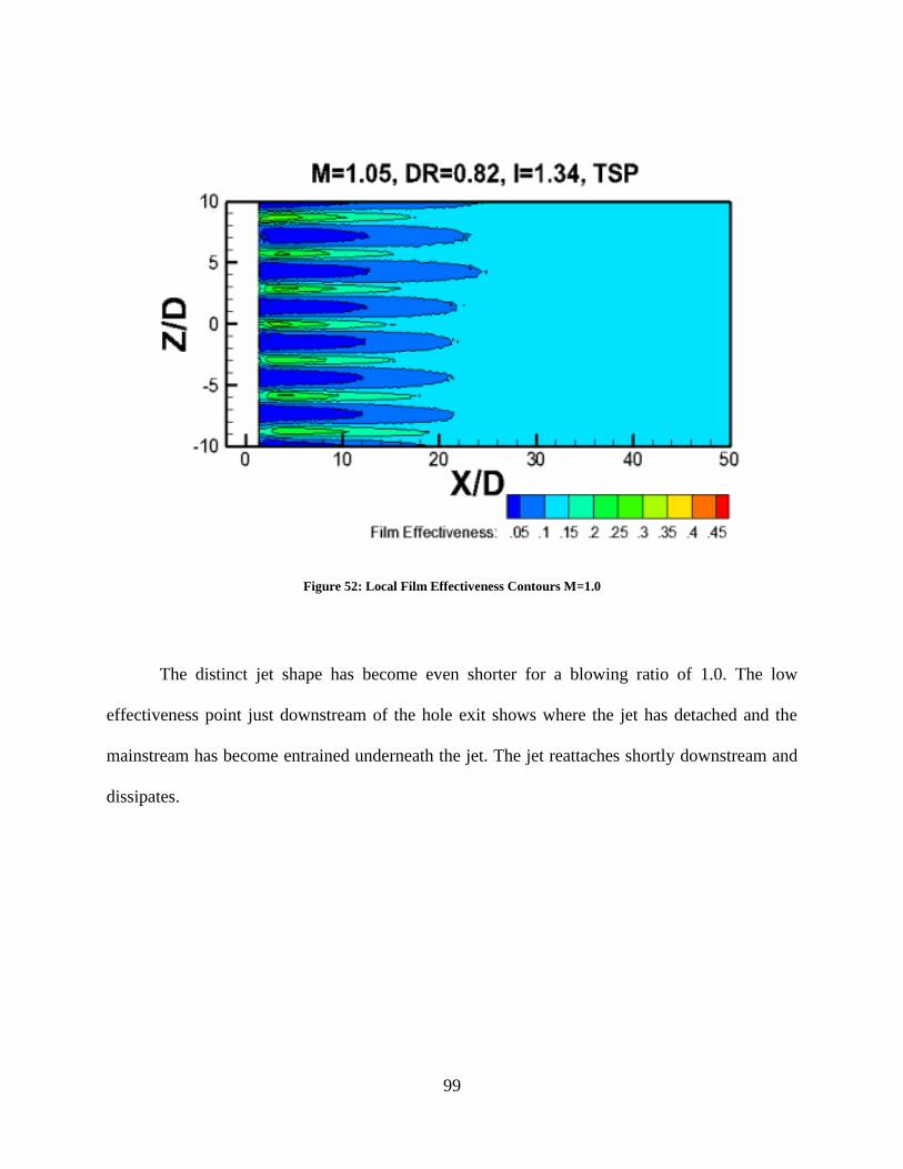
99
Figure 52: Local Film Effectiveness Contours M=1.0
The distinct jet shape has become even shorter for a blowing ratio of 1.0. The low
effectiveness point just downstream of the hole exit shows where the jet has detached and the
mainstream has become entrained underneath the jet. The jet reattaches shortly downstream and
dissipates.

100
Figure 53: Lateral Variation of Film Effectiveness M=1.0
Figure 53 represents the lateral variation in film effectiveness for a blowing ratio of 1.0.
The data sets donated a X/D value are a lateral slice of film effectiveness, the red lines in Figure
54 are the location of the local slices. The jets are highly uniform in magnitude, showing an even
distribution of coolant.
0
0.05
0.1
0.15
0.2
0.25
0.3
0.35
0.4
0.45
0.5
-25 -20 -15 -10 -5 0 5 10 15 20 25
Film
Eff
ecti
ven
ess
Z/D
X/D=2.5 X/D=5.0 X/D=10 X/D=15 Streamwise Average

101
Figure 54: Spanwise Local Effectiveness Trace Location
The black line in Figure 53, denoted streamwise average, is the average of the film
effectiveness at a given Z/D in the streamwise (X/D) direction. Figure 55 shows a diagram of the
procedure; the horizontal red line represents the streamwise average of a row of pixels. This
average is carried out at each Z/D. The result, in Figure 53 has only been shown for the film
holes used for the lateral averaging. The side three holes on each side are not included in lateral
averaging because of potential endwall effects. The streamwise average is laterally uniform. This
average shows the effect of the low effectiveness between the film holes on the total streamwise
film effectiveness value. Even with the increased jet spreading downstream, the film
effectiveness average is lower between the film holes.

102
Figure 55: Streamwise Average Diagram
Figure 56: Local Film Effectiveness Contours M=1.2

103
As the blowing ratio increases, the distinct visibility of film jet decreases in length. The
low effectiveness region between film jets increases in size, shown for a blowing ratio of 1.20 in
Figure 56. As the momentum flux ratio increases with blowing ratio, the jet spreading location
moves further upstream due to strong interaction between the jets and mainstream flow
(Goldstein et al., 1999).
Figure 57: Local Film Effectiveness Contours M=2.0
The jets begin spreading out only 12 diameters downstream of the hole exit at a blowing
ratio of 2.0, shown in Figure 57. The high effectiveness area further downstream is indicative of
jet reattachment. The high momentum coolant flow strongly interacts with the mainstream flow
and spreads the coolant film which flattens the effectiveness in the downstream areas.

104
Transpiration Cooling
The transpiration testing was performed at nominal blowing ratios of 0.05, 0.10, and
0.15. Comparisons are made to two correlations found in literature, 1) Goldstein (1965) and 2)
Kutateladze and Leont'ev (1963). These correlations are shown in Equation 10 and 11, shown
again below.
(
)
(10)
( (
)
)
(11)
Both of these correlations are found to fit data with blowing ratios below 0.03 very well.
Application to the current study is extrapolation at best; however they serve as a baseline to
compare against. The Goldstein correlation tends to over predict effectiveness. At low X values,
effectiveness values greater than unity are given. X is the stream wise distance started at the
leading edge of the porous slot. One of the assumptions of the Kutateladze correlation is unity
effectiveness at the point of injection (Goldstein, 1965).

105
The correlations serve to bound the measured effectiveness. The Goldstein correlation
has initial over prediction, a period of under prediction at approximately X/h of 50. The
Kutateladze correlation predicts the effectiveness well until further downstream where it under
predicts. The span averaged effectiveness for M = 0.05 is plotted log-log against X/Mh in Figure
58.
Figure 58: Transpiration Film Effectiveness M=0.05
An increase in surface protection by increased effectiveness is the result of increasing the
blowing ratio to 0.10. The correlations follow the same trend as for the low blowing case of 0.05.
The span averaged effectiveness values are shown in Figure 59. The decay rate in effectiveness
is more logarithmic for blowing ratio of 0.10.
0.01
0.1
1
10 100 1000 10000
Late
rally
Ave
rage
d F
ilm E
ffec
tive
nes
s
X/Mh
M=0.05
M=0.05 Goldstein
M=0.05 Kutateladze
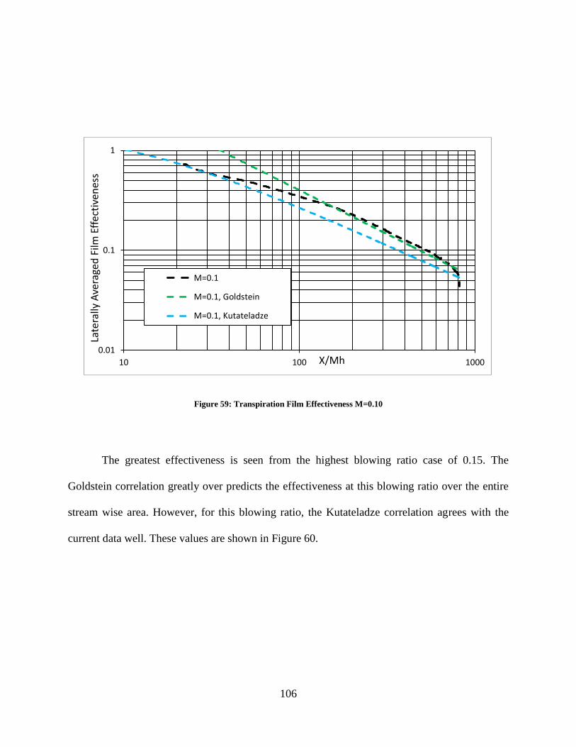
106
Figure 59: Transpiration Film Effectiveness M=0.10
The greatest effectiveness is seen from the highest blowing ratio case of 0.15. The
Goldstein correlation greatly over predicts the effectiveness at this blowing ratio over the entire
stream wise area. However, for this blowing ratio, the Kutateladze correlation agrees with the
current data well. These values are shown in Figure 60.
0.01
0.1
1
10 100 1000
Late
rally
Ave
rage
d F
ilm E
ffec
tive
nes
s
X/Mh
M=0.1
M=0.1, Goldstein
M=0.1, Kutateladze

107
Figure 60: Transpiration Film Effectiveness M=0.15
The three transpiration baselines are plotted with the two correlations for each case in
Figure 61. The curves essentially collapse down into a single mass. The slope of decay for the
experimental cases changes midway down the test surface, illustrated by surpassing the
correlations in effectiveness.
0.01
0.1
1
10 100 1000
Late
rally
Ave
rage
d F
ilm E
ffec
tive
nes
s
X/Mh
M=0.15
M=0.15, Goldstein
M=0.15, Kutateladze

108
Figure 61: Transpiration Film Effectiveness, Log-Log
Increasing the relative mass injected through the porous section results in greater surface
protection by increased effectiveness. The highest blowing ratio case shows the slowest decay
over the test surface; an effectiveness of greater than 0.08 is attained over the entire surface. A
greater increase in effectiveness is seen increasing from 0.05 to 0.10 than from 0.10 to 0.15
blowing ratio, shown in Figure 62. The shape of each curve is similar; the effect of increasing
blowing ratio serves to translate the curve vertically to higher effectiveness over the entire
surface.
0.01
0.1
1
10 100 1000 10000
Late
rally
Ave
rage
d F
ilm E
ffec
tive
nes
s
X/Mh
M=0.05M=0.05 GoldsteinM=0.05 KutateladzeM=0.1M=0.1, GoldsteinM=0.1, KutateladzeM=0.15M=0.15, Goldstein

109
Figure 62: Transpiration Laterally Averaged Effectiveness
The centerline effectiveness profiles appear in Figure 63 and are similar in shape and
magnitude to the laterally averaged film effectiveness profiles. The significance of this is the
injected film is distributed uniformly such that on average the lateral profile is close to the
centerline value. Local lateral non-uniformities which appear due to the porous structure are not
apparent in the lateral average.
0
0.2
0.4
0.6
0.8
1
0 10 20 30 40 50 60 70
Late
rally
Ave
rage
d F
ilm E
ffec
tive
nes
s
X/h
M=0.05, DR=0.851, I=0.003
M=0.094, DR=0.843, I=0.010
M=0.155, DR=0.841, I=0.029

110
Figure 63: Centerline Transpiration Effectiveness
Transpiration Numerical Versus Experimental
The CFD study did not capture the expected change in effectiveness due to the porosity
of the porous wall. However without further experimental results with the other porosity inserts,
an explicit conclusion cannot be made. The method of using a constant velocity boundary
condition to model a flow exiting a porous wall is a relatively poor indicator of cooling
performance by over predicting the film cooling effectiveness downstream of injection.
0
0.2
0.4
0.6
0.8
1
0 10 20 30 40 50 60 70
Cen
terl
ine
Effe
ctiv
enes
s
X/h
M=0.05, DR=0.851, I=0.003
M=0.094, DR=0.843, I=0.010
M=0.155, DR=0.841, I=0.029

111
Figure 64: CFD Versus Experimental Laterally Averaged Effectiveness
The velocity profile exiting from the porous wall is not uniform over the slot length.
Reducing the complexity down to a simple constant velocity increases the effectiveness
predicted. Figure 64 shows the CFD results with the 0.40 porosity insert experimental data. At
the same blowing ratio, the CFD predicts a much slower decay in effectiveness than the
experimental data.
0
0.2
0.4
0.6
0.8
1
0 10 20 30 40 50 60 70
Late
rally
Ave
rage
d F
ilm E
ffec
tive
nes
s
X/h
M=0.05
M=0.094
M=0.155
Case1
Case2
Case3
Case4
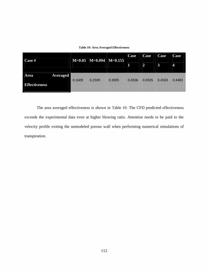
112
Table 10: Area Averaged Effectiveness
Case # M=0.05 M=0.094 M=0.155
Case
1
Case
2
Case
3
Case
4
Area Averaged
Effectiveness
0.1609 0.2509 0.3005 0.4506 0.4505 0.4503 0.4483
The area averaged effectiveness is shown in Table 10. The CFD predicted effectiveness
exceeds the experimental data even at higher blowing ratio. Attention needs to be paid to the
velocity profile exiting the unmodeled porous wall when performing numerical simulations of
transpiration.

113
Multi-Row Results
The first geometry, [30/45/14] serves as a validation case as it closely approximates a
geometry used by Mayle and Camarata (1975) with the addition of an adiabatic recovery region
devoid of holes. This geometry also serves to investigate the effect of including a compound
angle on a full coverage film array. The results given by Mayle and Camarata (1975) are given
on a streamwise averaged basis due to their use of a discrete point measurement technique while
the current experiment is shown as laterally averaged film effectiveness. There is little difference
between blowing ratio inside the film array for this geometry. Recovery region effectiveness is
dictated by the amount of mass preceding it; effectiveness and the reduction in decay rate are
governed by blowing ratio. Figure 65 shows the agreement in effectiveness between literature
data and the current experiment.
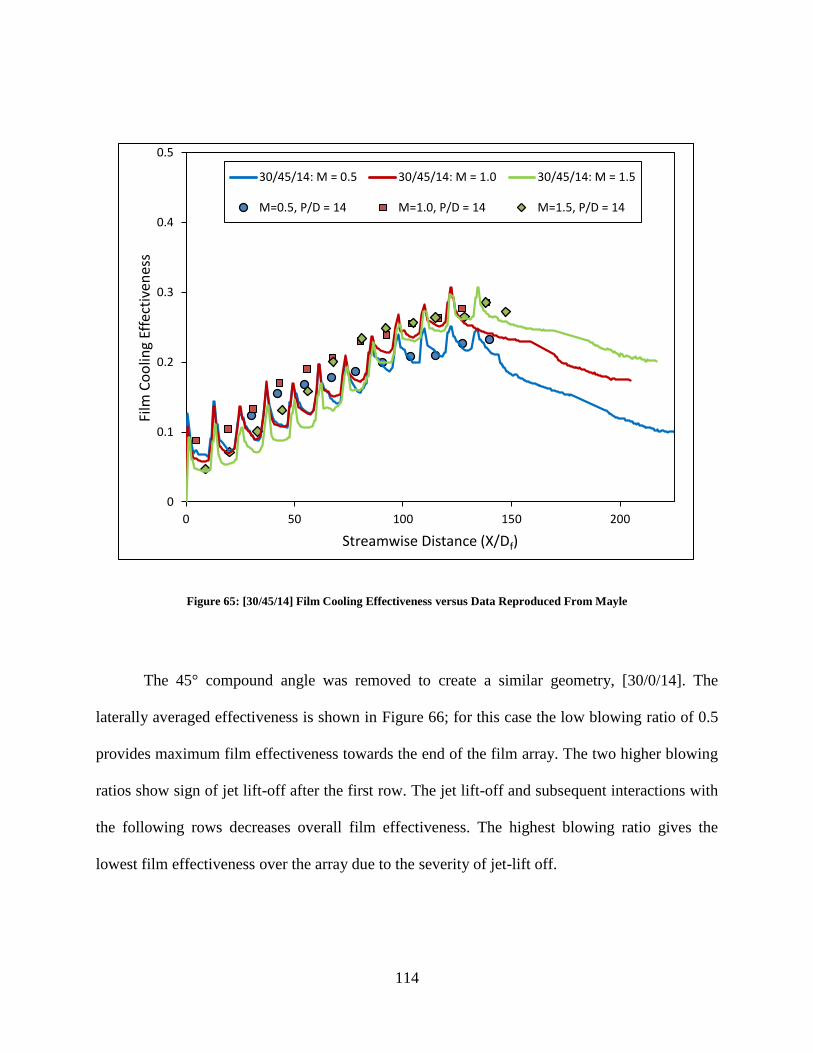
114
Figure 65: [30/45/14] Film Cooling Effectiveness versus Data Reproduced From Mayle
The 45° compound angle was removed to create a similar geometry, [30/0/14]. The
laterally averaged effectiveness is shown in Figure 66; for this case the low blowing ratio of 0.5
provides maximum film effectiveness towards the end of the film array. The two higher blowing
ratios show sign of jet lift-off after the first row. The jet lift-off and subsequent interactions with
the following rows decreases overall film effectiveness. The highest blowing ratio gives the
lowest film effectiveness over the array due to the severity of jet-lift off.
0
0.1
0.2
0.3
0.4
0.5
0 50 100 150 200
Film
Co
olin
g Ef
fect
iven
ess
Streamwise Distance (X/Df)
30/45/14: M = 0.5 30/45/14: M = 1.0 30/45/14: M = 1.5
M=0.5, P/D = 14 M=1.0, P/D = 14 M=1.5, P/D = 14

115
Figure 66: [30/0/14] Laterally Averaged Effectiveness
The [30/45/14] and [30/0/14] geometries are shown together at the low blowing ratio in
Figure 67. An equivalent amount of coolant is injected in each region of both arrays, however the
45° compound angle creates greater laterally averaged film effectiveness. The compound angle
creates a spreading effect that contributes to greater coverage of the surface. The net result is
greater effectiveness over the entire array at the same blowing ratio.
0
0.1
0.2
0.3
0.4
0.5
0 50 100 150 200
Late
rally
Ave
rage
d E
ffec
tive
nes
s
Streamwise Distance (X/Df)
30/0/14: M = 0.5
30/0/14: M = 1.0
30/0/14: M = 1.5

116
Figure 67: Effect of 45° Compound Angle
The periodic double row geometry [30/0/7] is shown in Figure 68. Between sets of rows
the effectiveness declines rapidly, however the effectiveness continues to increase over the film
array due to the injected mass. There is a discontinuity at the transition to the recovery region,
this is due to the different materials used between the test plate and recovery region, acrylic and
rohacell respectively. Thermal expansion differences between the plates created a minor
misalignment. The magnitude of effectiveness in the recovery region is questionable however the
decaying trend is not. Once again the low blowing ratio case is near optimal for this geometry.
The higher density hole spacing has the benefit of twice the geometric coverage over the
[30/0/14] and almost twice that of the [30/45/14] array. This allows the effectiveness
0
0.1
0.2
0.3
0.4
0.5
0 50 100 150 200
Late
rally
Ave
rage
d E
ffec
tive
nes
s
Streamwise Distance (X/Df)
30/45/14: M = 0.5
30/0/14: M = 0.5

117
immediately downstream of the array to be greater, yet decay at nearly the same rate. Hence, a
denser hole array spaced slightly farther, in this case, provides a more efficient use of coolant.
Figure 68: [30/0/7] Laterally Averaged Effectiveness
The transpiration geometry, [90/0/1], creates very high effectiveness peaks just
downstream of injection, as expected. The effectiveness quickly decreases downstream of
injection until the next row of transpiration are reached. The area between transpiration sections
shows an increase in effectiveness past each row due to the buildup of a coolant layer. The
discontinuity, not shown in Figure 69, in recovery region data is present here as well for the
0
0.1
0.2
0.3
0.4
0.5
0 50 100 150 200
Late
rally
Ave
rage
d E
ffec
tive
nes
s
Streamwise Distance (X/Df)
30/0/7: M = 0.5
30/0/7: M = 1.0
30/0/7: M = 1.5

118
same reason. The film effectiveness increases as blowing ratio and hence mass injected
increases. The momentum flux ratios for these cases are low such that the coolant film never
detaches from the flow surface.
Figure 69: [90/0/1] Laterally Averaged Effectiveness
The low blowing ratio cases between all geometries are compared in Figure 70. The
transpired array decays at a comparable rate to the discrete hole arrays despite the lower usage of
coolant, showing a more efficient usage per mass injected. The double row [30/0/7] shows an
advantage in film effectiveness over the full coverage arrays at low blowing.
0
0.1
0.2
0.3
0.4
0.5
0 50 100 150
Late
rally
Ave
rage
d E
ffec
tive
nes
s
Streamwise Distance (X/Df)
90/0/1: M = 0.06
90/0/1: M = 0.12
90/0/1: M = 0.18
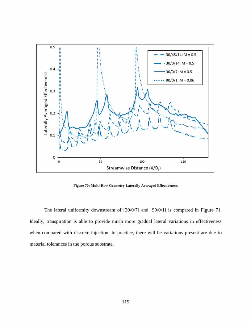
119
Figure 70: Multi-Row Geometry Laterally Averaged Effectiveness
The lateral uniformity downstream of [30/0/7] and [90/0/1] is compared in Figure 71.
Ideally, transpiration is able to provide much more gradual lateral variations in effectiveness
when compared with discrete injection. In practice, there will be variations present are due to
material tolerances in the porous substrate.
0
0.1
0.2
0.3
0.4
0.5
0 50 100 150
Late
rally
Ave
rage
d E
ffec
tive
nes
s
Streamwise Distance (X/Df)
30/45/14: M = 0.5
30/0/14: M = 0.5
30/0/7: M = 0.5
90/0/1: M = 0.06
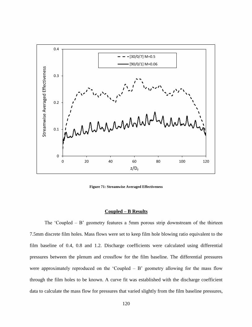
120
Figure 71: Streamwise Averaged Effectiveness
Coupled – B Results
The ‘Coupled – B’ geometry features a 5mm porous strip downstream of the thirteen
7.5mm discrete film holes. Mass flows were set to keep film hole blowing ratio equivalent to the
film baseline of 0.4, 0.8 and 1.2. Discharge coefficients were calculated using differential
pressures between the plenum and crossflow for the film baseline. The differential pressures
were approximately reproduced on the ‘Coupled – B’ geometry allowing for the mass flow
through the film holes to be known. A curve fit was established with the discharge coefficient
data to calculate the mass flow for pressures that varied slightly from the film baseline pressures,
0
0.1
0.2
0.3
0.4
0 20 40 60 80 100 120
Stre
amw
ise
Ave
rage
d E
ffec
tive
nes
s
z/Df
[30/0/7] M=0.5
[90/0/1] M=0.06

121
shown in Figure 72. The venturi flow meter installed upstream of the coolant plenum measures
the total mass flow through the coolant plenum; therefore the transpiration mass flow rate is also
known.
Figure 72: Mass Flow vs Differential Pressure
The local effectiveness contours for the three blowing ratios tested are shown in Figure
73 through Figure 75. The lateral non-uniformity is present in the same location as the
transpiration baseline. Therefore the reinstallation of the porous piece did not affect it, showing
that the non-uniformity is inherent in the porous piece. The areas of low effectiveness between
the discrete jets present in the film baseline are diminished due to the injection from
transpiration. The film and transpired flow mix into a constant coverage past 30 diameters
y = -9E-10x2 + 1E-05x + 0.0019 R² = 0.9916
0
0.005
0.01
0.015
0.02
0.025
0.03
0.035
0.04
0 1000 2000 3000 4000 5000 6000
Mas
s Fl
ow
(kg
/s)
dP (Pa.)
Cylindrical Holes@ Uinf=24m/s

122
downstream. Increasing the blowing ratio to 0.81 does not qualitatively increase effectiveness
versus the 0.4 case. The peaks of the jets extend a shorter distance downstream due to jet lift-off
present at this blowing ratio. The transpiration received the same blowing ratio for both cases,
causing a constant effectiveness downstream on the test surface. The highest blowing case of
1.21 resulted in a high transpiration blowing ratio of 0.21; the result of which is an increase in
non-uniformity at a Z/D of 0. High effectiveness extends downstream of the porous section
followed by noticeable jet lift-off. Reattachment occurs followed by significant mixing between
the transpired and discrete film. With this number of contours, the flow becomes homogenous
past 30 diameters downstream, except for the non-uniformity at Z/D of 0.
Figure 73: Local Effectiveness Contours MCYL = 0.41 MTRAN =0.074

123
Figure 74: Local Effectiveness Contours MCYL =0.81 MTRAN=0.075
Figure 75: Local Effectiveness Contours MCYL = 1.22 MTRAN =0.21
124
The laterally averaged effectiveness profiles for the Coupled-B geometry are shown in
Figure 76. The transpiration strip is downstream of the film holes in this arrangement. The
different sets of blowing ratios tested give effectiveness curves similar in magnitude and slope.
The lowest film blowing ratio case, Mcyl = 0.4, surpasses the higher film blowing ratio of 0.8
case past an X/D of 5. This can easily be attributed to the film blowing ratio at the critical value
between staying attached to the wall and being lifted from the surface. This results in low
effectiveness. Since the two cases have the same transpiration blowing ratio, they reach the same
effectiveness value far downstream of the injection location. The highest blowing ratio case
reaches the highest effectiveness over the entire test surface. The first 10 diameters of
effectiveness appears to be dominated by the transpired flow. Far downstream the increased
thermal capacity of the larger film injected mass as well as increased turbulent mixing from the
higher momentum film flow results in the effectiveness being dominated by the discrete hole
injection.

125
Figure 76: Laterally Averaged Effectiveness Coupled-B
When plotted with the two baseline cases that approximately match the coupled case, it is
apparent that the transpiration effectiveness does dominate the effectiveness value. Figure 77
shows the lowest blowing ratio cases. The discrete hole film begins to dominate in the
downstream region where the discrete jets have mixed and spread out. From a linear
superposition perspective, the region just downstream of injection is not indicative of positive
effect on effectiveness from coupling the two technologies. However, far downstream appears to
have validity for a linear superposition approach. If the blowing ratios between the three cases
were the same, past a X/D of 35, the linear superposition technique could be valid. The net effect
is an effectiveness profile that reaches transpiration levels just downstream and exceeds both
film and transpiration further downstream.
0
0.2
0.4
0.6
0.8
1
0 5 10 15 20 25 30 35 40 45 50
Late
rally
Ave
rage
d E
ffec
tive
nes
s
X/D
Mcyl=0.4, Mtran=0.074, h/D=2/3, O/D=-1, P/D=3
Mcyl=0.8, Mtran=0.075, h/D=2/3, O/D=-1, P/D=3
Mcyl=1.2, Mtran=0.21, h/D=2/3, O/D=-1, P/D=3

126
Figure 77: Laterally Averaged Effectiveness Comparison, Mcyl=0.4, Mtran=0.07
The next set of blowing ratios is shown in Figure 78. The point that discrete hole film
injection surpasses the transpiration effectiveness has been shifted downstream, due to the lower
effectiveness of the Mcyl blowing ratio case. The coupled case once again matches and surpasses
the transpiration effectiveness. Only far downstream would a linear superposition possibly be
valid.
0
0.2
0.4
0.6
0.8
1
0 10 20 30 40 50
Late
rally
Ave
rage
d F
ilm E
ffec
tive
nes
s
X/D
M=0.094 Transpiration
M 0.41 Film Hole
Mcyl=0.4, Mtran=0.07, h/D=2/3, O/D=-1, P/D=3

127
Figure 78: Laterally Averaged Effectiveness Comparison, Mcyl=0.8, Mtran=0.08
The highest transpiration blowing ratio fell short of the coupled transpiration blowing
ratio, 0.155 versus 0.21 respectively. With this magnitude greater transpiration blowing ratio,
one would expect greater effectiveness just downstream of injection. However this is not the
case, the coupled geometry once again matches the transpiration effectiveness regardless of the
greater amount of mass injected. As the blowing ratios are increased, the point which film
cooling surpasses transpiration cooling effectiveness is shifted further downstream. The coupled
case approximately stops decaying past a X/D of 15, due to the increasing trend in effectiveness
of the film injection.
0
0.2
0.4
0.6
0.8
1
0 10 20 30 40 50
Late
rally
Ave
rage
d F
ilm E
ffec
tive
nes
s
X/D
M=0.094 Transpiration
M 0.79 Film Hole
Mcyl=0.8, Mtran=0.08, h/D=2/3, O/D=-1, P/D=3

128
Figure 79: Laterally Averaged Effectiveness Comparison, Mcyl=1.2, Mtran=0.21
Coupled – A Results
The Coupled-A geometry features a 5mm porous strip upstream of a row of 7.5mm
discrete film holes. This is a shift of the permeable section by 4-5 hole diameters upstream
compared to the previous Coupled-B geometry. This significant shift in the permeable section
can be seen to only marginally affect the surface downstream. Also very similar is the film
effectiveness following the coupled source despite the large shift in permeable section location.
At large downstream distances, greater than thirty, the effectiveness following each coupled
source collapse on one another showing the downstream effectiveness is governed by the
discrete row alone; transpiration no longer governs cooling at large downstream distances. The
laterally averaged effectiveness for the Coupled-A geometry is shown in Figure 80.
0
0.2
0.4
0.6
0.8
1
0 10 20 30 40 50
Late
rally
Ave
rage
d F
ilm E
ffec
tive
nes
s
X/D
M=0.155 Transpiration
M=1.21 Film Hole
Mcyl=1.2, Mtran=0.21, h/D=2/3, O/D=-1, P/D=3

129
Figure 80: Laterally Averaged Effectiveness Coupled-A
The magnitude of effectiveness is similar for the three cases. The cylindrical blowing
ratio cases of 0.4 and 0.8 show nearly identical effectiveness until an X/D of 20. Since a
cylindrical blowing ratio 0.8 is shown to have characteristically low effectiveness, therefore the
initial high effectiveness is entirely due to the transpiration injection. The highest blowing ratio
case has negligibly higher initial effectiveness than the two lower blowing cases despite having
twice the amount of transpired flow. The film flow serves to increase effectiveness past an X/D
of 20 from the thermal capacity of the larger mass of coolant and the increased turbulent mixing
with the mainstream.
Local effectiveness contours for the three cases are shown in Figure 81 through Figure
83. From these contours, it is seen that the transpiring flow appears to have less effect on the film
0
0.2
0.4
0.6
0.8
1
0 10 20 30 40 50
Late
rally
Ave
rage
d E
ffec
tive
nes
s
X/D
Mcyl=0.4, Mtran=0.11, h/D=2/3, O/D=1, P/D=3
Mcyl=0.8, Mtran=0.12, h/D=2/3, O/D=1, P/D=3
Mcyl=1.2, Mtran=0.22, h/D=2/3, O/D=1, P/D=3
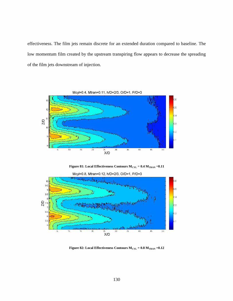
130
effectiveness. The film jets remain discrete for an extended duration compared to baseline. The
low momentum film created by the upstream transpiring flow appears to decrease the spreading
of the film jets downstream of injection.
Figure 81: Local Effectiveness Contours MCYL = 0.4 MTRAN =0.11
Figure 82: Local Effectiveness Contours MCYL = 0.8 MTRAN =0.12
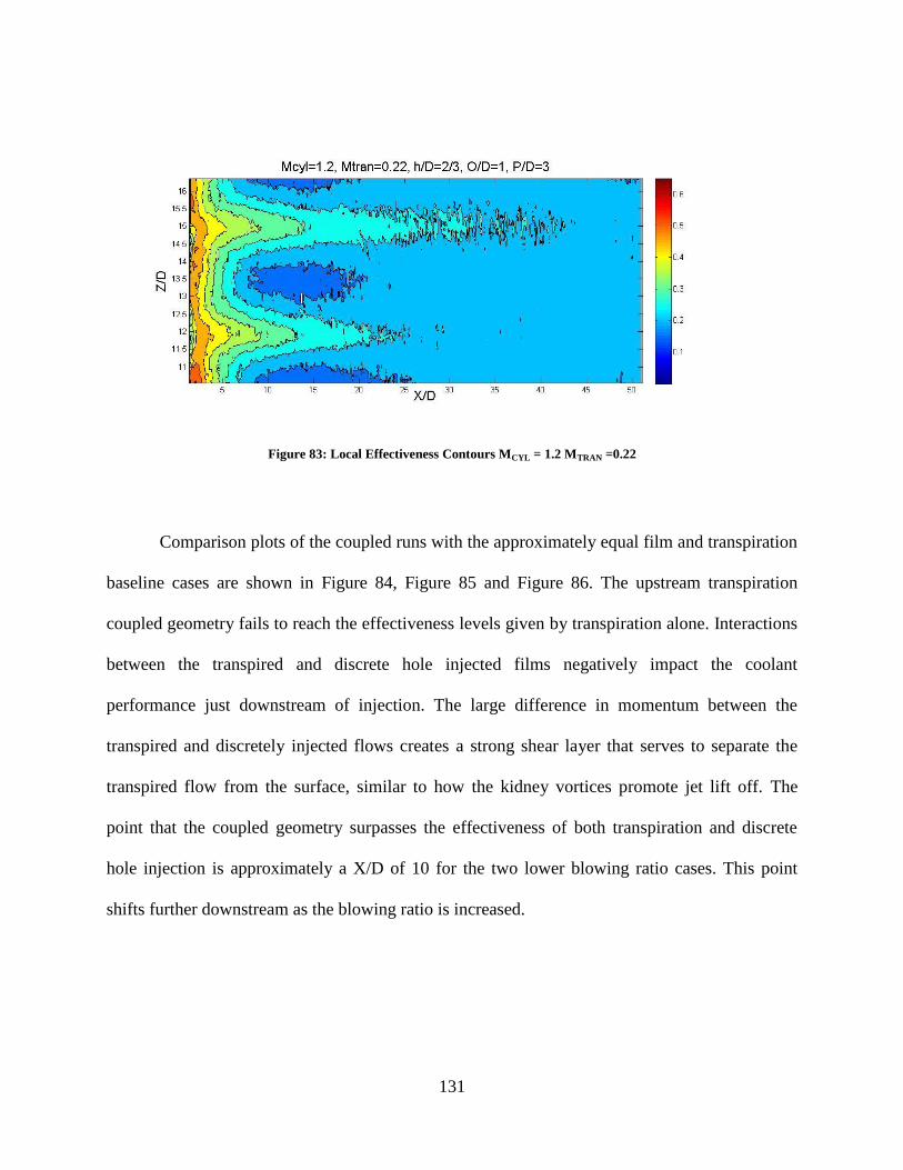
131
Figure 83: Local Effectiveness Contours MCYL = 1.2 MTRAN =0.22
Comparison plots of the coupled runs with the approximately equal film and transpiration
baseline cases are shown in Figure 84, Figure 85 and Figure 86. The upstream transpiration
coupled geometry fails to reach the effectiveness levels given by transpiration alone. Interactions
between the transpired and discrete hole injected films negatively impact the coolant
performance just downstream of injection. The large difference in momentum between the
transpired and discretely injected flows creates a strong shear layer that serves to separate the
transpired flow from the surface, similar to how the kidney vortices promote jet lift off. The
point that the coupled geometry surpasses the effectiveness of both transpiration and discrete
hole injection is approximately a X/D of 10 for the two lower blowing ratio cases. This point
shifts further downstream as the blowing ratio is increased.
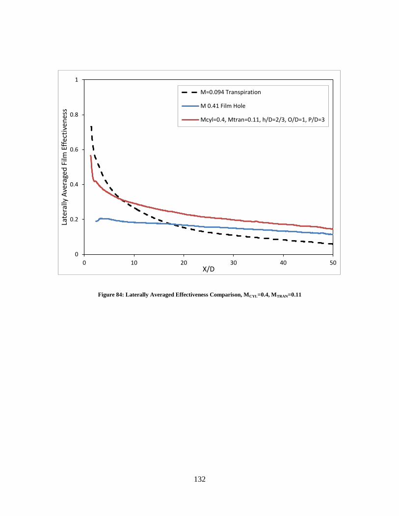
132
Figure 84: Laterally Averaged Effectiveness Comparison, MCYL=0.4, MTRAN=0.11
0
0.2
0.4
0.6
0.8
1
0 10 20 30 40 50
Late
rally
Ave
rage
d F
ilm E
ffec
tive
nes
s
X/D
M=0.094 Transpiration
M 0.41 Film Hole
Mcyl=0.4, Mtran=0.11, h/D=2/3, O/D=1, P/D=3

133
Figure 85: Laterally Averaged Effectiveness Comparison, MCYL=0.8, MTRAN=0.12
0
0.2
0.4
0.6
0.8
1
0 10 20 30 40 50
Late
rally
Ave
rage
d F
ilm E
ffec
tive
nes
s
X/D
M=0.094 Transpiration
M 0.79 Film Hole
Mcyl=0.8, Mtran=0.12, h/D=2/3, O/D=1, P/D=3

134
Figure 86: Laterally Averaged Effectiveness Comparison, MCYL=1.2, MTRAN=0.22
Coupled Comparison
The laterally averaged effectiveness for both coupled geometries is shown in Figure 87.
Coupled-A is depicted as solid lines (O/D=1) while Coupled-B is shown as dashed lines (O/D=-
1). The Coupled-A geometry has the transpiration strip upstream of the film holes while
Coupled-B has it downstream. The difference in geometry causes two distinct trends, the
Coupled-B geometry has greater initial effectiveness due to the downstream placement of the
transpiration segment, and far downstream the discrete hole injection clearly dominates the
effectiveness. Since the discrete hole blowing ratios were able to be consistently kept the same,
0
0.2
0.4
0.6
0.8
1
0 10 20 30 40 50
Late
rally
Ave
rage
d F
ilm E
ffec
tive
nes
s
X/D
M=0.155 Transpiration
M=1.21 Film Hole
Mcyl=1.2, Mtran=0.22, h/D=2/3, O/D=1, P/D=3

135
the far downstream effectiveness for the cases between geometries with the same blowing ratio
reach the same effectiveness value. It appears that having the transpiration segment downstream
of the discrete holes allows for the discrete jets to entrain transpired flow instead of the
mainstream flow.
Figure 87: Laterally Averaged Effectiveness Coupled Geometries
Further analysis must be performed to compare the relative amount of losses generated
from either coupled geometry. Comparisons from an application perspective would then be more
possible.
0
0.2
0.4
0.6
0.8
1
0 5 10 15 20 25 30 35 40 45 50
Late
rally
Ave
rage
d E
ffec
tive
nes
s
X/D
Mcyl=0.4, Mtran=0.11, h/D=2/3, O/D=1, P/D=3Mcyl=0.8, Mtran=0.12, h/D=2/3, O/D=1, P/D=3Mcyl=1.2, Mtran=0.22, h/D=2/3, O/D=1, P/D=3Mcyl=0.4, Mtran=0.07, h/D=2/3, O/D=-1, P/D=3Mcyl=0.8, Mtran=0.08, h/D=2/3, O/D=-1, P/D=3Mcyl=1.2, Mtran=0.21, h/D=2/3, O/D=-1, P/D=3

136
CHAPTER 6: CONCLUSION
Ex Supra
The first chapter introduced basic theory behind gas turbine operation and explained the
need for advancing turbine cooling technologies. The two distinct technologies, discrete hole
film cooling and transpiration cooling were introduced. The current work was introduced as the
coupling of those two technologies for the improvement of cooling performance.
The second chapter described some of the history of film cooling and transpiration and
detailed the governing parameters as well as fundamental concepts behind those two
technologies. Included is an extensive literature review of research regarded as directly
applicable to the current work.
The third chapter incorporated correlations found in literature in order to find an optimal
starting point for a coupled discrete hole and transpiration cooling system. The two coupled
geometries were described in detail.
The fourth chapter detailed the experiment wind tunnel and measurements techniques
used to characterize the performance of the baseline, coupled, and multi-row geometries. The
hot-wire anemometry setup was detailed and calculation methods for turbulence length scales
were explained. The temperature sensitive paint measurement technique luminescent process is
overviewed. The data acquisition and processing systems utilized along with the image
registration process is given.
The fifth chapter incorporated experiment validation as well as experiment results. The
discrete hole and transpiration baselines were validated against literature data and correlations
137
from literature respectively. The baseline data was found to be valid and of excellent resolution.
The coupled geometries were analyzed based on film effectiveness. The local effectiveness as
well as laterally averaged effectiveness was presented and detailed. Both geometries increased
effectiveness over the baseline cases; giving credibility to incorporating either geometry based
on design constraints. However having the transpiring section downstream of the film holes did
increase effectiveness downstream of injection to the levels of transpiration. The upstream
transpiring section geometry did not match the transpiration level of effectiveness just
downstream of injection.
De Futuro
The current study is just the first step in the research of coupling these cooling
technologies. The increase in cooling performance has been established, now the physics behind
how the two flows interact needs to be analyzed. Flow imaging technology such as PIV or LDV
should be used to visualize the interactions between the transpiring and discretely injected flows.
Furthermore, experimental data needs to be compared with CFD simulations in order to create
design tools for implementation. Additionally, with the progression of laser additive
manufacturing, airfoil shapes can be created with discrete holes and porous sections. The
inclusion of surface curvature as well as varying levels of turbulence intensity needs to be
experimentally performed. From a mechanical standpoint, the effect on thermo-mechanical
stresses from having both transpiration and film cooling needs to be addressed.

138
REFERENCES
Baldauf, S., Scheurlen, M., Schulz, A., & Wittig, S. (2002a). Correlation of Film-Cooling
Effectiveness From Thermographic Measurements at Enginelike Conditions. Journal of
Turbomachinery, 124(4), 686-698. doi: 10.1115/1.1504443
Baldauf, S., Scheurlen, M., Schulz, A., & Wittig, S. (2002b). Heat Flux Reduction From Film
Cooling and Correlation of Heat Transfer Coefficients From Thermographic
Measurements at Enginelike Conditions. Journal of Turbomachinery, 124(4), 699-709.
doi: 10.1115/1.1505848
Barrett, M. J., & Hollingsworth, D. K. (2001). On the calculation of length scales for turbulent
heat transfer correlation. Journal of Heat Transfer, 123(5), 878-883.
Bergeles, G., Gosman, A. D., & Launder, B. E. (1977). Near - Field Character of Jet a
Discharged Through a Wall at 30 Degrees to a Mainstream. AIAA Journal, 15(4), 499-
504.
Brown, A., & Saluja, C. L. (1979). Film cooling from a single hole and a row of holes of variable
pitch to diameter ratio. International Journal of Heat and Mass Transfer, 22(4), 525-534.
doi: 10.1016/0017-9310(79)90056-5
Cal, R. B., Wang, X., & Castillo, L. (2005). Transpired turbulent boundary layers subject to
forced convection and external pressure gradients. Journal of Heat Transfer, 127, 194.
Crawford, M. E., Kays, W. M., & Moffat, R. J. (1980). Full-coverage film cooling. Part I:
Comparison of heat transfer data for three injection angles. Journal of Engineering for
Power, 102, 1000-1005.
Denton, J. D. (1993). The 1993 IGTI Scholar Lecture: Loss Mechanisms in Turbomachines.
Journal of Turbomachinery, 115(4), 621-656. doi: 10.1115/1.2929299
Dryden, H. L., Shubauer, G. B., Moch, W. C., & Skramstad, H. K. (1937). Measurements of
intensity and scale of wind-tunnel turbulence and their relation to the critical Reynolds
number of spheres: National Advisory Committee for Aeronautics.
Eckert, E. R. G. (1952). Transpiration and film cooling. Paper presented at the Heat-Transfer
Symposium, Ann Arbor Engineering-Research Institute, University of Michigan.
Eckert, E. R. G., & Cho, H. H. (1994). Transition from transpiration to film cooling.
International Journal of Heat and Mass Transfer, 37, Supplement 1(0), 3-8. doi:
10.1016/0017-9310(94)90003-5

139
Eckert, E. R. G., & Livingood, J. N. B. (1954). Comparison of effectiveness of convection,
transpiration and film cooling methods with air as coolant. NACA TN 3010(Journal
Article).
Forth, C. J. P., Loftus, P. J., & Jones, T. V. (1985). The Effect of Density Ratio on the Film
Cooling of a Flat Plate. Heat Transfer and Cooling in Gas Turbines, AGARD-CP-390,
Paper 10(Journal Article).
Foster, N. W., & Lampard, D. (1980). The Flow and Film Cooling Effectiveness Following
Injection Through a Row of Holes. ASME J. Eng. Power, 102(Journal Article), 584-588.
Fraser, R., Pack, C. J., & Santavicca, D. A. (1986). An LDV system for turbulence length scale
measurements. Experiments in Fluids, 4(3), 150-152.
Georgiou, D. P., & Louis, J. F. (1985). The Transpired Turbulent Boundary Layer in Various
Pressure Gradients and the Blow-Off Condition. Journal of Engineering for Gas Turbines
and Power, 107(3), 636-641. doi: 10.1115/1.3239783
Goldstein, R. J. (1965). Film Cooling Effectiveness With Injection Through a Porous Section.
Journal of Heat Transfer, 87(Journal Article), 353.
Goldstein, R. J. (1969). Film Cooling Following Injection Through Inclined Circular Tubes (Vol.
NASA CR 72612).
Goldstein, R. J. (1971). Film Cooling. In F. I. Thomas & P. H. James (Eds.), Advances in Heat
Transfer (Vol. Volume 7, pp. 321-379): Elsevier.
Goldstein, R. J., Eckert, E. R. G., & Burggraf, F. (1974). Effects of hole geometry and density on
three-dimensional film cooling. International Journal of Heat and Mass Transfer, 17(5),
595-607. doi: 10.1016/0017-9310(74)90007-6
Goldstein, R. J., Jin, P., & Olson, R. L. (1999). Film Cooling Effectiveness and Mass/Heat
Transfer Coefficient Downstream of One Row of Discrete Holes. Journal of
Turbomachinery, 121(2), 225-232. doi: 10.1115/1.2841305
Gutmark, E. J., & Grinstein, F. F. (1999). Flow Control with Non Circular Jets Annual Review of
Fluid Mechanics, 31(1), 239-272.
Han, J.-C., Sandip, D., & Srinath, E. (2000). Gas Turbine Heat Transfer and Cooling
Technology. New York: Taylor & Francis.
Haven, B. A., & Kurosaka, M. (1997). Kidney and anti-kidney vortices in crossflow jets. Journal
of Fluid Mechanics, 352(Journal Article), 27-64.
Hinze, J. (1975). Turbulence (2nd ed.): McGraw-Hill.
140
Holm, D. D. (2005). Taylor’s Hypothesis, Hamilton’s Principle, and the LANS-α Model for
Computing Turbulence. Los Alamos Science, 29(1).
Johnson, P. L., Nguyen, C. Q., Ho, S. H., & Kapat, J. S. (2010). Sensitivity Analysis of Domain
Considerations for Numerical Simulations of Film Cooling. ASME Conference
Proceedings, 2010(49408), 285-300. doi: 10.1115/ihtc14-23241
Kays, W. M. (1972). Heat transfer to the transpired turbulent boundary layer. International
Journal of Heat and Mass Transfer, 15(5), 1023-1044. doi: 10.1016/0017-
9310(72)90237-2
Kline, S. J., & McClintock, F. A. (1953). Describing uncertainties in single-sample experiments.
Mechanical engineering, 75(1), 3-8.
Kutateladze, S. S., & Leont'ev, A. I. (1963). The Heat Curtain in the Turbulent Boundary Layer
of a Gas. High Temperature, 1(Journal Article).
Lewalle, J., & Ashpis, D. E. (2004). Estimation of Time Scales in Unsteady Flows in a
Turbomachinery Rig: Final Report NASA-TM-2004-209452, NASA Lewis Research
Center, Cleveland, Ohio, USA.
Liu, T., & Sullivan, J. P. (2005). Pressure and Temperature Sensitive Paints. Berlin: Springer.
Mayle, R. E., & Camarata, F. J. (1975). Multihole cooling film effectiveness and heat transfer.
Journal of Heat Transfer, 97, 534.
Moretti, P., & Kays, W. M. (1965). Heat transfer to a turbulent boundary layer with varying free-
stream velocity and varying surface temperature—an experimental study. International
Journal of Heat and Mass Transfer, 8(9), 1187-1202.
Morris, S. C., & Foss, J. F. (2003). Turbulent boundary layer to single-stream shear layer: the
transition region. Journal of Fluid Mechanics, 494, 187-221.
Natsui, G., Johnson, P. L., Torrance, M. C., Ricklick, M. A., & Kapat, J. S. (2011). The Effect of
Transpiration On Discrete Injection For Film Cooling. Paper presented at the ASME
Turbo Expo 2011, Vancouver, Canada.
Natsui, G., Torrance, M. C., Miller, M. W., Ricklick, M. A., & Kapat, J. S. (2011). Multi-Row
Transpiration Cooling with Comparison to Discrete Arrays. Paper presented at the IGTC
2011, Osaka, Japan.
Pedersen, D. R., Eckert, E. R. G., & Goldstein, R. J. (1977). Film Cooling With Large Density
Differences Between the Mainstream and the Secondary Fluid Measured by the Heat-
Mass Transfer Analogy. Journal of Heat Transfer, 99(4), 620-627. doi:
10.1115/1.3450752

141
Pietrzyk, J. R., Bogard, D. G., & Crawford, M. E. (1989). Hydrodynamic Measurements of Jets
in Crossflow for Gas Turbine Film Cooling Applications. Journal of Turbomachinery,
111(2), 139-145.
Pietrzyk, J. R., Bogard, D. G., & Crawford, M. E. (1990). Effects of Density Ratio on the
Hydrodynamics of Film Cooling. Journal of Turbomachinery, 112(3), 437-443.
Polezhaev, J. (1997). The Transpiration Cooling for Blades of High Temperatures Gas Turbine.
International Symposium on Advance Energy Conversion Systems and Related
Technologies, 38(10), 1123-1133. doi: 10.1016/s0196-8904(96)00142-2
Quinn, W. R. (1992). Turbulent free jet flows issuing from sharp-edged rectangular slots: The
influence of slot aspect ratio. Experimental Thermal and Fluid Science, 5(2), 203-215.
Sellers, J. P. (1963). Gaseous film cooling with multiple injection stations. AIAA J, 1(9), 2154-
2156.
Sinha, A. K., Bogard, D. G., & Crawford, M. E. (1991). Film-Cooling Effectiveness
Downstream of a Single Row of Holes With Variable Density Ratio. Journal of
Turbomachinery, 113(3), 442-449.
Welch, P. (1967). The use of fast Fourier transform for the estimation of power spectra: a
method based on time averaging over short, modified periodograms. Audio and
Electroacoustics, IEEE Transactions on, 15(2), 70-73.
Wilcock, R. C., Young, J. B., & Horlock, J. H. (2005). The Effect of Turbine Blade Cooling on
the Cycle Efficiency of Gas Turbine Power Cycles. Journal of Engineering for Gas
Turbines and Power, 127(1), 109-120. doi: 10.1115/1.1805549