Coupled Tanks Experiment for MATLAB /Simulink Users

INSTRUCTOR WORKBOOKCoupled Tanks Experiment for MATLAB /Simulink Users

Standardized for ABET* Evaluation Criteria

Developed by:Jacob Apkarian, Ph.D., Quanser

Hervé Lacheray, M.A.SC., QuanserAmin Abdossalami, M.A.SC., Quanser

CApTIvATE. MOTIvATE. GRAdUATE.

Quanser educational solutions are powered by:

Course material complies with:

* ABET Inc., is the recognized accreditor for college and university programs in applied science, computing, engineering, and technology; and has provided leadership and quality assurance in higher education for over 75 years.

© 2013 Quanser Inc., All rights reserved.

Quanser Inc.119 Spy CourtMarkham, OntarioL3R [email protected]: 1-905-940-3575Fax: 1-905-940-3576

Printed in Markham, Ontario.

For more information on the solutions Quanser Inc. offers, please visit the web site at:http://www.quanser.com

This document and the software described in it are provided subject to a license agreement. Neither the software nor this document may beused or copied except as specified under the terms of that license agreement. All rights are reserved and no part may be reproduced, stored ina retrieval system or transmitted in any form or by any means, electronic, mechanical, photocopying, recording, or otherwise, without the priorwritten permission of Quanser Inc.

ACKNOWLEDGEMENTSQuanser, Inc. would like to thank the following contributors:

Dr. Hakan Gurocak, Washington State University Vancouver, USA, for his help to include embedded outcomes assessment, and

Dr. K. J. Åström, Lund University, Lund, Sweden for his immense contributions to the curriculum content.

COUPLED TANKS Workbook - Student Version 2

http://www.quanser.com

CONTENTS1 Introduction 4

2 Modeling 52.1 Background 52.2 Pre-Lab Questions 10

3 Tank 1 Level Control 113.1 Background 113.2 Pre-Lab Questions 143.3 Lab Experiments 153.4 Results 17

4 Tank 2 Level Control 194.1 Background 194.2 Pre-Lab Questions 214.3 Lab Experiments 224.4 Results 25

5 System Requirements 265.1 Overview of Files 275.2 Setup for Tanks 1 Control Simulation 275.3 Setup for Tanks 2 Control Simulation 285.4 Setup for Implementing Tank 1 Control 285.5 Setup for Implementing Tank 2 Level Control 28

6 Lab Report 306.1 Template for Tank 1 Level Control Report 306.2 Template for Tank 2 Level Control Report 316.3 Tips for Report Format 32

COUPLED TANKS Workbook - Student Version v 1.0

1 INTRODUCTIONThe Coupled Tanks plant is a "Two-Tank" module consisting of a pump with a water basin and two tanks. The twotanks are mounted on the front plate such that flow from the first (i.e. upper) tank can flow, through an outlet orificelocated at the bottom of the tank, into the second (i.e. lower) tank. Flow from the second tank flows into the mainwater reservoir. The pump thrusts water vertically to two quick-connect orifices "Out1" and "Out2". The two systemvariables are directly measured on the Coupled-Tank rig by pressure sensors and available for feedback. They arenamely the water levels in tanks 1 and 2. A more detailed description is provided in [5]. To name a few, industrialapplications of such Coupled-Tank configurations can be found in the processing system of petro-chemical, papermaking, and/or water treatment plants.

During the course of this experiment, youwill become familiar with the design and pole placement tuning of Proportional-plus-Integral-plus-Feedforward-based water level controllers. In the present laboratory, the Coupled-Tank systemis used in two different configurations, namely configuration #1 and configuration #2, as described in [5]. In config-uration #1, the objective is to control the water level in the top tank, i.e., tank #1, using the outflow from the pump.In configuration #2, the challenge is to control the water level in the bottom tank, i.e. tanks #2, from the water flowcoming out of the top tank. Configuration #2 is an example of state coupled system.

Topics Covered

• How to mathematically model the Coupled-Tank plant from first principles in order to obtain the two open-looptransfer functions characterizing the system, in the Laplace domain.

• How to linearize the obtained non-linear equation of motion about the quiescent point of operation.

• How to design, through pole placement, a Proportional-plus-Integral-plus-Feedforward-based controller for theCoupled-Tank system in order for it to meet the required design specifications for each configuration.

• How to implement each configuration controller(s) and evaluate its/their actual performance.

Prerequisites

In order to successfully carry out this laboratory, the user should be familiar with the following:

1. See the system requirements in Section 5 for the required hardware and software.

2. Transfer function fundamentals, e.g., obtaining a transfer function from a differential equation.

3. Familiar with designing PID controllers.

4. Basics of Simulinkr.

5. Basics of QUARCr.


2 MODELING

2.1 Background

2.1.1 Configuration #1 System Schematics

A schematic of the Coupled-Tank plant is represented in Figure 2.1, below. The Coupled-Tank system's nomen-clature is provided in Appendix A. As illustrated in Figure 2.1, the positive direction of vertical level displacement isupwards, with the origin at the bottom of each tank (i.e. corresponding to an empty tank), as represented in Figure3.2.

Figure 2.1: Schematic of Coupled Tank in Configuration #1.

2.1.2 Configuration #1 Nonlinear Equation of Motion (EOM)

In order to derive the mathematical model of your Coupled-Tank system in configuration #1, it is reminded that thepump feeds into Tank 1 and that tank 2 is not considered at all. Therefore, the input to the process is the voltage tothe pump VP and its output is the water level in tank 1, L1, (i.e. top tank).

The purpose of the present modelling session is to provide you with the system's open-loop transfer function, G1(s),which in turn will be used to design an appropriate level controller. The obtained Equation of Motion, EOM, shouldbe a function of the system's input and output, as previously defined.


Therefore, you should express the resulting EOM under the following format:

∂L1

∂t= f(L1, Vp)

where f denotes a function.

In deriving the Tank 1 EOM the mass balance principle can be applied to the water level in tank 1, i.e.,

At1∂L1

∂t= Fi1 − Fo1 (2.1)

where At1 is the area of Tank 1. Fi1 and Fo1 are the inflow rate and outflow rate, respectively. The volumetric inflowrate to tank 1 is assumed to be directly proportional to the applied pump voltage, such that:

Fi1 = KpVp

Applying Bernoulli's equation for small orifices, the outflow velocity from tank 1, vo1, can be expressed by the followingrelationship:

vo1 =√2gL1

2.1.3 Configuration #1 EOM Linearization and Transfer Func-tion

In order to design and implement a linear level controller for the tank 1 system, the open-loop Laplace transferfunction should be derived. However by definition, such a transfer function can only represent the system's dynamicsfrom a linear differential equation. Therefore, the nonlinear EOM of tank 1 should be linearized around a quiescentpoint of operation. By definition, static equilibrium at a nominal operating point (Vp0, L10) is characterized by theTank 1 level being at a constant position L10 due to a constant water flow generated by constant pump voltage Vp0.

In the case of the water level in tank 1, the operating range corresponds to small departure heights, L11, and smalldeparture voltages, Vp1, from the desired equilibrium point (Vp0, L10). Therefore, L1 and Vp can be expressed asthe sum of two quantities, as shown below:

L1 = L10 + L11, Vp = Vp0 + Vp1 (2.2)

The obtained linearized EOM should be a function of the system's small deviations about its equilibrium point(Vp0, L10). Therefore, one should express the resulting linear EOM under the following format:

∂

∂tL11 = f(L11, Vp1) (2.3)


Example: Linearizing a Two-Variable FunctionHere is an example of how to linearize a two-variable nonlinear function called f(z). Variable z is defined

z⊤ = [z1 z2]

and f(z) is to be linearized about the operating point

z0⊤ = [a b]


The linearized function is

fz = f(z0) +

(∂f(z)

∂z1

) ∣∣∣∣z=z0

(z1 − a) +

(∂f(z)

∂z2

) ∣∣∣∣z=z0

(z2 − b)

For a function, f , of two variables, L1 and Vp, a first-order approximation for small variations at a point (L1, Vp) =(L10, Vp0) is given by the following Taylor's series approximation:

∂2

∂L1∂Vpf (L1, Vp) ∼= f (L10, Vp0) +

(∂

∂L1f (L10, Vp0)

)+ (L1 − L10)

(∂

∂Vpf (L10, Vp0)

)(Vp − Vp0) (2.4)

Transfer FunctionFrom the linear equation of motion, the system's open-loop transfer function in the Laplace domain can be definedby the following relationship:

G1(s) =L11(s)

Vp1(s)(2.5)

The desired open-loop transfer function for the Coupled-Tank's tank 1 system is the following:

G1(s) =Kdc1

τ1s+ 1(2.6)

where Kdc1 is the open-loop transfer function DC gain, and τ1 is the time constant.

As a remark, it is obvious that linearized models, such as the Coupled-Tank tank 1's voltage-to-level transfer function,are only approximate models. Therefore, they should be treated as such and used with appropriate caution, that isto say within the valid operating range and/or conditions. However for the scope of this lab, Equation 2.5 is assumedvalid over the pump voltage and tank 1 water level entire operating range, Vp_peak and L1_max, respectively.

2.1.4 Configuration #2 System Schematics

A schematic of the Coupled-Tank plant is represented in Figure 2.2, below. The Coupled-Tank system's nomen-clature is provided in Appendix A. As illustrated in Figure 2.2, the positive direction of vertical level displacement isupwards, with the origin at the bottom of each tank (i.e. corresponding to an empty tank), as represented in Figure2.2.

2.1.5 Configuration #2, Nonlinear Equation of Motion (EOM)

This section explains the mathematical model of your Coupled-Tank system in configuration #2, as described inReference [1]. It is reminded that in configuration #2, the pump feeds into tank 1, which in turn feeds into tank 2.As far as tank 1 is concerned, the same equations as the ones explained in Section 2.1.2 and Section 2.1.3 willapply. However, the water level Equation Of Motion (EOM) in tank 2 still needs to be derived. The input to the tank2 process is the water level, L1, in tank 1 (generating the outflow feeding tank 2) and its output variable is the waterlevel, L2, in tank 2 (i.e. bottom tank). The purpose of the present modelling session is to guide you with the system'sopen-loop transfer function, G2(s), which in turn will be used to design an appropriate level controller. The obtainedEOM should be a function of the system's input and output, as previously defined.

Therefore, you should express the resulting EOM under the following format:

∂L2

∂t= f(L2, L1)


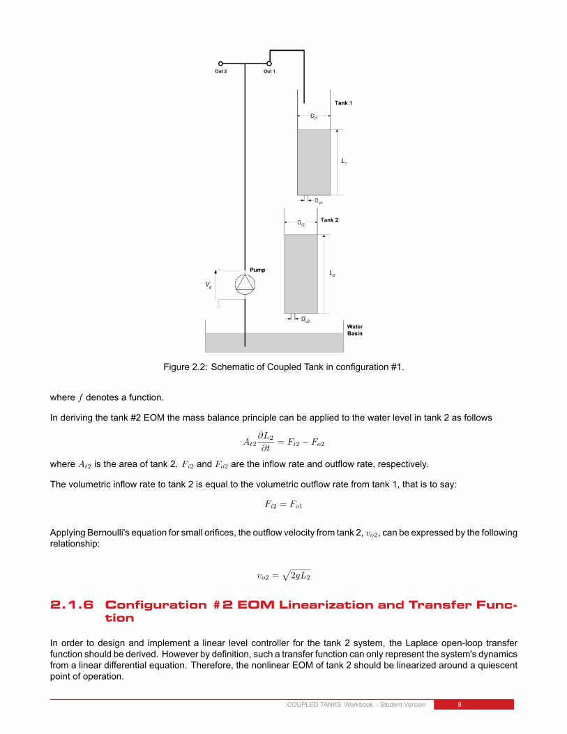
Figure 2.2: Schematic of Coupled Tank in configuration #1.


In deriving the tank #2 EOM the mass balance principle can be applied to the water level in tank 2 as follows

At2∂L2

∂t= Fi2 − Fo2

where At2 is the area of tank 2. Fi2 and Fo2 are the inflow rate and outflow rate, respectively.

The volumetric inflow rate to tank 2 is equal to the volumetric outflow rate from tank 1, that is to say:

Fi2 = Fo1

Applying Bernoulli's equation for small orifices, the outflow velocity from tank 2, vo2, can be expressed by the followingrelationship:

vo2 =√2gL2

2.1.6 Configuration #2 EOM Linearization and Transfer Func-tion

In order to design and implement a linear level controller for the tank 2 system, the Laplace open-loop transferfunction should be derived. However by definition, such a transfer function can only represent the system's dynamicsfrom a linear differential equation. Therefore, the nonlinear EOM of tank 2 should be linearized around a quiescentpoint of operation.


In the case of the water level in tank 2, the operating range corresponds to small departure heights, L11 and L21,from the desired equilibrium point (L10, L20). Therefore, L2 and L1 can be expressed as the sum of two quantities,as shown below:

L2 = L20 + L21, L1 = L10 + L11 (2.7)

The obtained linearized EOM should be a function of the system's small deviations about its equilibrium point(L20, L10). Therefore, you should express the resulting linear EOM under the following format:

∂

∂tL21 = f(L11, L21) (2.8)


For a function, f , of two variables, L1 and L2, a first-order approximation for small variations at a point (L1, L2) =(L10, L20) is given by the following Taylor's series approximation:

∂2

∂L1∂L2f (L1, L2) ∼= f (L10, L20) +

(∂

∂L1f (L10, L20)

)+ (L1 − L10)

(∂

∂L2f (L10, L20)

)(L2 − L20) (2.9)

Transfer FunctionFrom the linear equation of motion, the system's open-loop transfer function in the Laplace domain can be definedby the following relationship:

G2(s) =L21(s)

L11(s)(2.10)

the desired open-loop transfer function for the Coupled-Tank's tank 2 system, such that:

G2(s) =Kdc2

τ2s+ 1(2.11)

where Kdc2 is the open-loop transfer function DC gain, and τ2 is the time constant.

As a remark, it is obvious that linearized models, such as the Coupled-Tank's tank 2 level-to-level transfer function,are only approximate models. Therefore, they should be treated as such and used with appropriate caution, that is tosay within the valid operating range and/or conditions. However for the scope of this lab, Equation 2.10 is assumedvalid over tank 1 and tank 2 water level entire range of motion, L1_max and L2_max, respectively.


2.2 Pre-Lab Questions

Answer the following questions:

1. Using the notations and conventions described in Figure 2 derive the Equation Of Motion (EOM) characterizingthe dynamics of tank 1. Is the tank 1 system's EOM linear?Hint: The outflow rate from tank 1, Fo1, can be expressed by:

Fo1 = Ao1vo1 (2.12)

2. The nominal pump voltage Vp0 for the pump-tank 1 pair can be determined at the system's static equilibrium.By definition, static equilibrium at a nominal operating point (Vp0, L10) is characterized by the water in tank1 being at a constant position level L10 due to the constant inflow rate generated by Vp0. Express the staticequilibrium voltage Vp0 as a function of the system's desired equilibrium level L10 and the pump flow constantKp. Using the system's specifications given in the Coupled Tanks User Manual ([5]) and the desired designrequirements in Section 3.1.1, evaluate Vp0 parametrically.

3. Linearize tank 1 water level's EOM found in Question #1 about the quiescent operating point (Vp0, L10).

4. Determine from the previously obtained linear equation of motion, the system's open-loop transfer function inthe Laplace domain as defined in Equation 2.5 and Equation 2.6. Express the open-loop transfer function DCgain, Kdc1 , and time constant, τ1, as functions of L10 and the system parameters. What is the order and typeof the system? Is it stable? Evaluate Kdc1 and τ1 according to system's specifications given in the CoupledTanks User Manual ([5]) and the desired design requirements in Section 3.1.1.

5. Using the notations and conventions described in Figure 2.2, derive the Equation Of Motion (EOM) character-izing the dynamics of tank 2. Is the tank 2 system's EOM linear?Hint: The outflow rate from tank 2, Fo2, can be expressed by:

Fo2 = Ao2vo2 (2.13)

6. The nominal water level L10 for the tank1-tank2 pair can be determined at the system's static equilibrium. Bydefinition, static equilibrium at a nominal operating point (L10, L20) is characterized by the water in tank 2 beingat a constant position level L20 due to the constant inflow rate generated from the top tank by L10. Expressthe static equilibrium level L10 as a function of the system's desired equilibrium level L20 and the system'sparameters. Using the system's specifications given in the Coupled Tanks User Manual ([5]) and the desireddesign requirements in Section 4.1.1, evaluate L10.

7. Linearize tank 2 water level's EOM found in Question #5 about the quiescent operating point (L10, L20).

8. Determine from the previously obtained linear equation of motion, the system's open-loop transfer function inthe Laplace domain, as defined in Equation 2.10 and Equation 2.11. Express the open-loop transfer functionDC gain, Kdc2 , and time constant, τ2, as functions of L10, L20, and the system parameters. What is the orderand type of the system? Is it stable? Evaluate Kdc2 and τ2 according to system's specifications given in theCoupled Tanks User Manual ([5]) and the desired design requirements in Section 4.1.1.


3 TANK 1 LEVEL CONTROL

3.1 Background

3.1.1 Specifications

In configuration #1, a control is designed to regulate the water level (or height) of tank #1 using the pump voltage. Thecontrol is based on a Proportional-Integral-Feedforward scheme (PI-FF). Given a ±1 cm square wave level setpoint(about the operating point), the level in tank 1 should satisfy the following design performance requirements:

1. Operating level in tank 1 at 15 cm: L10 = 15 cm.

2. Percent overshoot less than 10%: PO1 ≤ 11 %.

3. 2% settling time less than 5 seconds: ts_1 ≤ 5.0 s.

4. No steady-state error: ess = 0 cm.

3.1.2 Tank 1 Level Controller Design: Pole Placement

For zero steady-state error, tank 1 water level is controlled by means of a Proportional-plus-Integral (PI) closed-loopscheme with the addition of a feedforward action, as illustrated in Figure 3.1, below, the voltage feedforward actionis characterized by:

Vp_ff = Kff_1√

Lr_1 (3.1)

and

Vp = Vp1 + Vp_ff (3.2)

As it can be seen in Figure 3.1, the feedforward action is necessary since the PI control system is designed tocompensate for small variations (a.k.a. disturbances) from the linearized operating point (Vp0, L10). In other words,while the feedforward action compensates for the water withdrawal (due to gravity) through tank 1 bottom outletorifice, the PI controller compensates for dynamic disturbances.

Figure 3.1: Tank 1 Water Level PI-plus-Feedforward Control Loop.


The open-loop transfer functionG1(s) takes into account the dynamics of the tank 1 water level loop, as characterizedby Equation 2.5. However, due to the presence of the feedforward loop, G1(s) can also be written as follows:

G1(s) =L1(s)

Vp1(s)(3.3)

3.1.3 Second-Order Response

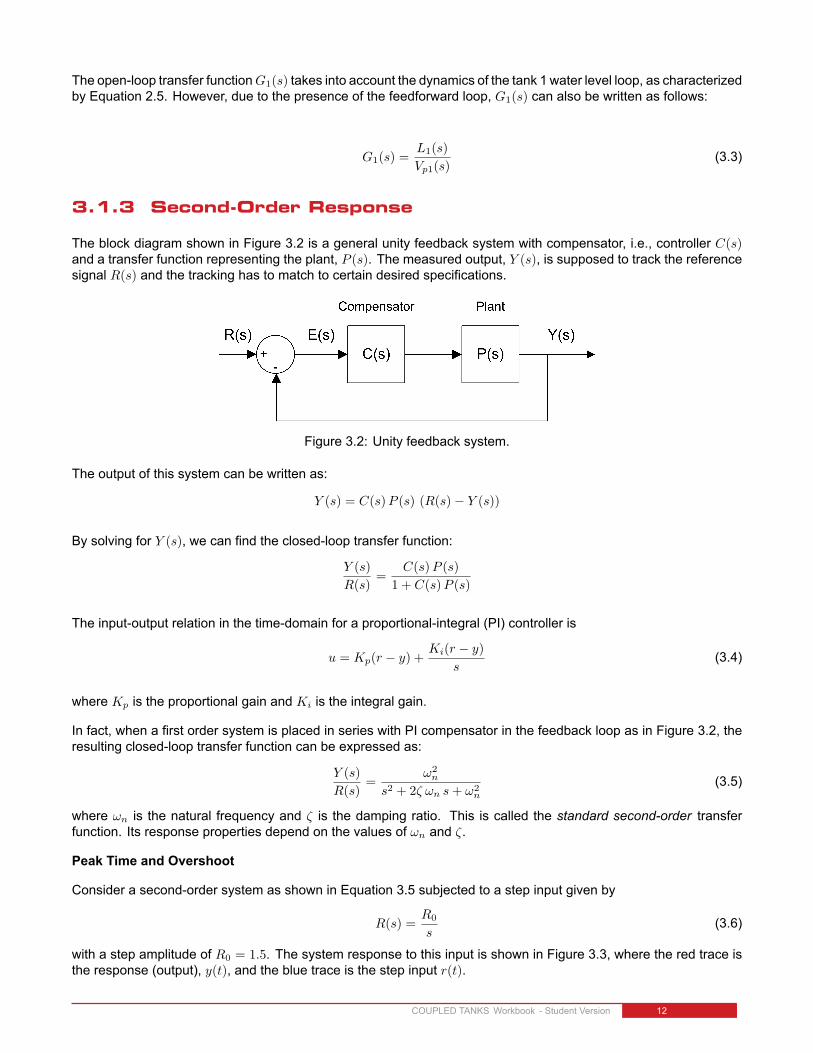
The block diagram shown in Figure 3.2 is a general unity feedback system with compensator, i.e., controller C(s)and a transfer function representing the plant, P (s). The measured output, Y (s), is supposed to track the referencesignal R(s) and the tracking has to match to certain desired specifications.

Figure 3.2: Unity feedback system.

The output of this system can be written as:

Y (s) = C(s)P (s) (R(s)− Y (s))

By solving for Y (s), we can find the closed-loop transfer function:

Y (s)

R(s)=

C(s)P (s)

1 + C(s)P (s)

The input-output relation in the time-domain for a proportional-integral (PI) controller is

u = Kp(r − y) +Ki(r − y)

s(3.4)

where Kp is the proportional gain and Ki is the integral gain.

In fact, when a first order system is placed in series with PI compensator in the feedback loop as in Figure 3.2, theresulting closed-loop transfer function can be expressed as:

Y (s)

R(s)=

ω2n

s2 + 2ζ ωn s+ ω2n

(3.5)

where ωn is the natural frequency and ζ is the damping ratio. This is called the standard second-order transferfunction. Its response properties depend on the values of ωn and ζ.

Peak Time and Overshoot

Consider a second-order system as shown in Equation 3.5 subjected to a step input given by

R(s) =R0

s(3.6)

with a step amplitude of R0 = 1.5. The system response to this input is shown in Figure 3.3, where the red trace isthe response (output), y(t), and the blue trace is the step input r(t).


Figure 3.3: Standard second-order step response.

The maximum value of the response is denoted by the variable ymax and it occurs at a time tmax. For a responsesimilar to Figure 3.3, the percent overshoot is found using

PO =100 (ymax −R0)

R0(3.7)

From the initial step time, t0, the time it takes for the response to reach its maximum value is

tp = tmax − t0 (3.8)

This is called the peak time of the system.

In a second-order system, the amount of overshoot depends solely on the damping ratio parameter and it can becalculated using the equation

PO = 100 e

(− π ζ√

1−ζ2

)(3.9)

The peak time depends on both the damping ratio and natural frequency of the system and it can be derived as

tp =π

ωn

√1− ζ2

(3.10)

Tank 1 level response 2% Settling Time can be expressed as follows:

ts =4

ζω(3.11)

Generally speaking, the damping ratio affects the shape of the response while the natural frequency affects thespeed of the response.



1. Analyze tank 1 water level closed-loop system at the static equilibrium point (Vp0, L10) and determine andevaluate the voltage feedforward gain, Kff_1, as defined by Equation 3.1.

2. Using tank 1 voltage-to-level transfer function G1(s) determined in Section 2.2 and the control scheme blockdiagram illustrated in Figure 3.1, derive the normalized characteristic equation of the water level closed-loopsystem.Hint#1: The feedforward gain Kff_1 does not influence the system characteristic equation. Therefore, thefeedforward action can be neglected for the purpose of determining the denominator of the closed-loop transferfunction. Block diagram reduction can be carried out.Hint#2: The system's normalized characteristic equation should be a function of the PI level controller gains,Kp_1, and Ki_1, and system's parameters, Kdc_1 and τ1.

3. By identifying the controller gains Kp_1 and Ki_1, fit the obtained characteristic equation to the second-orderstandard form expressed below:

s2 + 2ζ1ωn1s+ ω2n1 = 0 (3.12)

Determine Kp_1 and Ki1 as functions of the parameters ωn1, ζ1, Kdc_1, and τ1 using Equation 3.5.

4. Determine the numerical values forKp_1 andKi_1 in order for the tank 1 system to meet the closed-loop desiredspecifications, as previously stated.


3.3 Lab Experiments

3.3.1 Objectives

• Tune through pole placement the PI-plus-feedforward controller for the actual water level in tank 1 of theCoupled-Tank system.

• Implement the PI-plus-feedforward control loop for the actual Coupled-Tank's tank 1 level.

• Run the obtained PI-plus-feedforward level controller and compare the actual response against the controllerdesign specifications.

• Run the system's simulation simultaneously, at every sampling period, in order to compare the actual andsimulated level responses.

3.3.2 Tank 1 Level Control Simulation

Experimental Setup

The s_tanks_1 Simulinkr diagram shown in Figure 3.4 is used to perform tank 1 level control simulation exercisesin this laboratory.

Figure 3.4: Simulink model used to simulate PI-FF control on Coupled Tanks system in configuration #1.

IMPORTANT: Before you can conduct these simulations, you need to make sure that the lab files are configuredaccording to your setup. If they have not been configured already, then you need to go to Section 5 to configure thelab files first.

Follow this procedure:

1. Enter the proportional, integral, and feedforward gain control gains found in Section 3.2 in Matlab as Kp_1,Ki_1, and Kff_1.

2. To generate a step reference, go to the Signal Generator block and set it to the following:

• Signal type = square• Amplitude = 1• Frequency = 0.02 Hz

3. Set the Amplitude (cm) gain block to 1 to generate a square wave goes between ±1 cm.


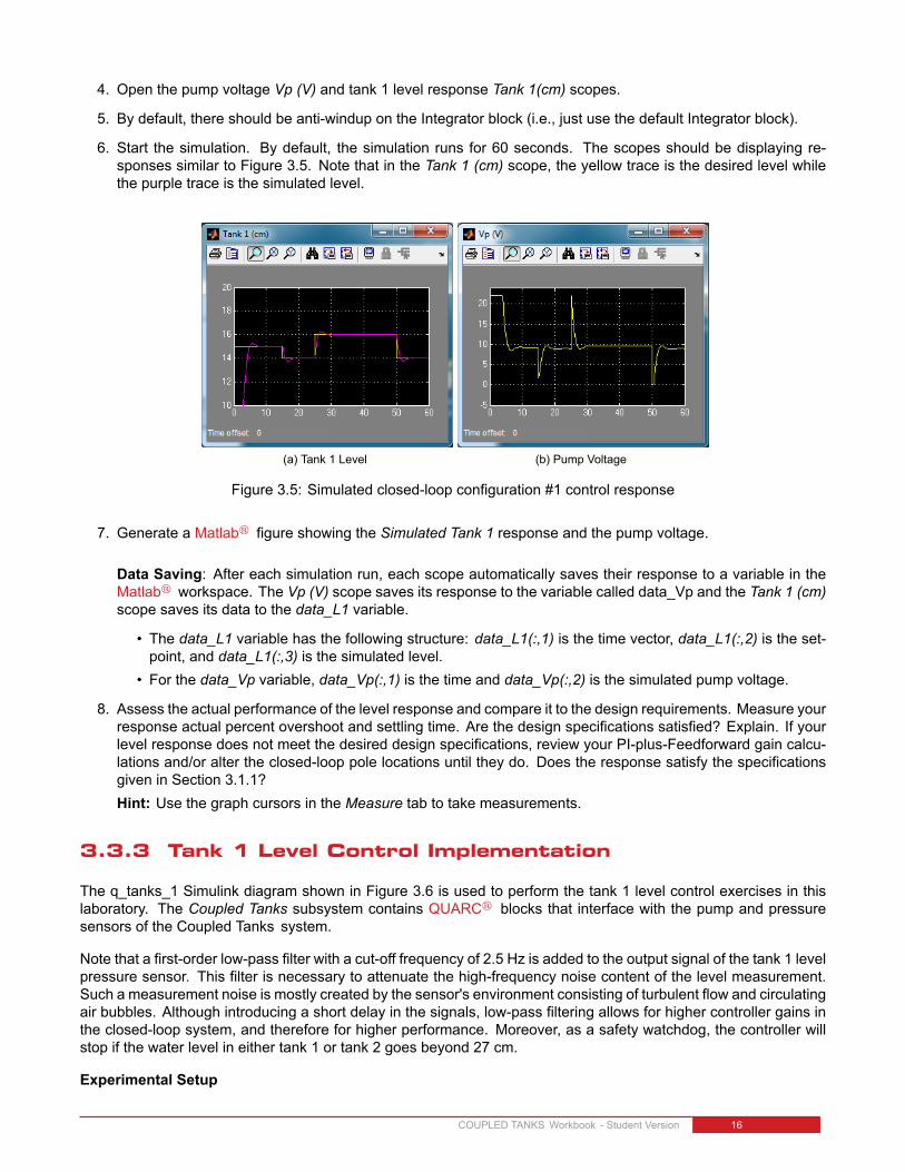
4. Open the pump voltage Vp (V) and tank 1 level response Tank 1(cm) scopes.

5. By default, there should be anti-windup on the Integrator block (i.e., just use the default Integrator block).

6. Start the simulation. By default, the simulation runs for 60 seconds. The scopes should be displaying re-sponses similar to Figure 3.5. Note that in the Tank 1 (cm) scope, the yellow trace is the desired level whilethe purple trace is the simulated level.

(a) Tank 1 Level (b) Pump Voltage

Figure 3.5: Simulated closed-loop configuration #1 control response

7. Generate a Matlabr figure showing the Simulated Tank 1 response and the pump voltage.

Data Saving: After each simulation run, each scope automatically saves their response to a variable in theMatlabr workspace. The Vp (V) scope saves its response to the variable called data_Vp and the Tank 1 (cm)scope saves its data to the data_L1 variable.

• The data_L1 variable has the following structure: data_L1(:,1) is the time vector, data_L1(:,2) is the set-point, and data_L1(:,3) is the simulated level.

• For the data_Vp variable, data_Vp(:,1) is the time and data_Vp(:,2) is the simulated pump voltage.

8. Assess the actual performance of the level response and compare it to the design requirements. Measure yourresponse actual percent overshoot and settling time. Are the design specifications satisfied? Explain. If yourlevel response does not meet the desired design specifications, review your PI-plus-Feedforward gain calcu-lations and/or alter the closed-loop pole locations until they do. Does the response satisfy the specificationsgiven in Section 3.1.1?Hint: Use the graph cursors in the Measure tab to take measurements.

3.3.3 Tank 1 Level Control Implementation

The q_tanks_1 Simulink diagram shown in Figure 3.6 is used to perform the tank 1 level control exercises in thislaboratory. The Coupled Tanks subsystem contains QUARCr blocks that interface with the pump and pressuresensors of the Coupled Tanks system.

Note that a first-order low-pass filter with a cut-off frequency of 2.5 Hz is added to the output signal of the tank 1 levelpressure sensor. This filter is necessary to attenuate the high-frequency noise content of the level measurement.Such a measurement noise is mostly created by the sensor's environment consisting of turbulent flow and circulatingair bubbles. Although introducing a short delay in the signals, low-pass filtering allows for higher controller gains inthe closed-loop system, and therefore for higher performance. Moreover, as a safety watchdog, the controller willstop if the water level in either tank 1 or tank 2 goes beyond 27 cm.

Experimental Setup


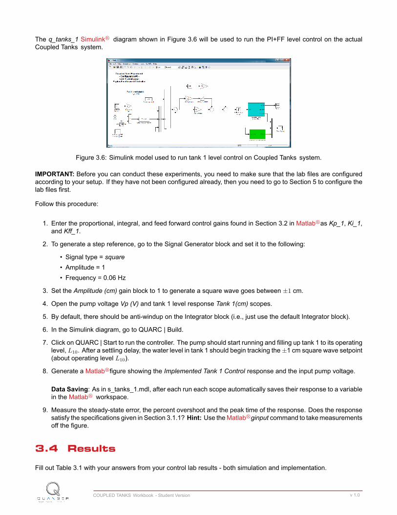
The q_tanks_1 Simulinkr diagram shown in Figure 3.6 will be used to run the PI+FF level control on the actualCoupled Tanks system.

Figure 3.6: Simulink model used to run tank 1 level control on Coupled Tanks system.

IMPORTANT: Before you can conduct these experiments, you need to make sure that the lab files are configuredaccording to your setup. If they have not been configured already, then you need to go to Section 5 to configure thelab files first.


1. Enter the proportional, integral, and feed forward control gains found in Section 3.2 in Matlabras Kp_1, Ki_1,and Kff_1.

2. To generate a step reference, go to the Signal Generator block and set it to the following:


3. Set the Amplitude (cm) gain block to 1 to generate a square wave goes between ±1 cm.

4. Open the pump voltage Vp (V) and tank 1 level response Tank 1(cm) scopes.

5. By default, there should be anti-windup on the Integrator block (i.e., just use the default Integrator block).

6. In the Simulink diagram, go to QUARC | Build.

7. Click on QUARC | Start to run the controller. The pump should start running and filling up tank 1 to its operatinglevel, L10. After a settling delay, the water level in tank 1 should begin tracking the±1 cm square wave setpoint(about operating level L10).

8. Generate a Matlabrfigure showing the Implemented Tank 1 Control response and the input pump voltage.

Data Saving: As in s_tanks_1.mdl, after each run each scope automatically saves their response to a variablein the Matlabr workspace.

9. Measure the steady-state error, the percent overshoot and the peak time of the response. Does the responsesatisfy the specifications given in Section 3.1.1? Hint: Use theMatlabrginput command to takemeasurementsoff the figure.

3.4 Results

Fill out Table 3.1 with your answers from your control lab results - both simulation and implementation.


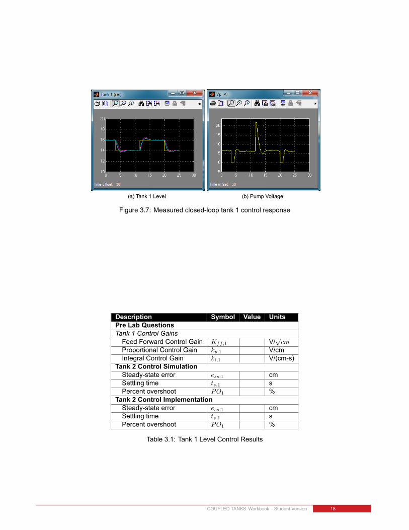
(a) Tank 1 Level (b) Pump Voltage

Figure 3.7: Measured closed-loop tank 1 control response

Description Symbol Value UnitsPre Lab QuestionsTank 1 Control GainsFeed Forward Control Gain Kff,1 V/

√cm

Proportional Control Gain kp,1 V/cmIntegral Control Gain ki,1 V/(cm-s)

Tank 2 Control SimulationSteady-state error ess,1 cmSettling time ts,1 sPercent overshoot PO1 %

Tank 2 Control ImplementationSteady-state error ess,1 cmSettling time ts,1 sPercent overshoot PO1 %

Table 3.1: Tank 1 Level Control Results


4 TANK 2 LEVEL CONTROL

4.1 Background

4.1.1 Specifications

In configuration #2, the pump feeds tank 1 and tank 1 feeds tank 2. The designed closed-loop system is to controlthe water level in tank 2 (i.e. the bottom tank) from the water flow coming out of tank 1, located above it. Similarlyto configuration #1, the control scheme is based on a Proportional-plus-Integral-plus-Feedforward law.

In response to a desired ± 1 cm square wave level setpoint from tank 2 equilibrium level position, the water heightbehaviour should satisfy the following design performance requirements:

1. Tank 2 operating level at 15 cm: L20 = 15 cm.

2. Percent overshoot should be less than or equal to 10%: PO2 ≤ 10.0 %.

3. 2% settling time less than 20 seconds: ts,2 ≤ 20.0 s.

4. No steady-state error: ess,2 = 0 cm.

4.1.2 Tank 2 Level Controller Design: Pole Placement

For zero steady-state error, tank 1 water level is controlled by means of a Proportional-plus-Integral (PI) closed-loopscheme with the addition of a feedforward action, as illustrated in Figure 4.1, below.

In the block diagram depicted in Figure 4.1, the water level in tank 1 is controlled by means of the closed-loop systempreviously designed in Section 3.1. This is represented by the tank 1 closed-loop transfer function defined below:

T1(s) =L1(s)

Lr_1(s)(4.1)

Such a subsystem represents an inner (or nested) level loop. In order to achieve a good overall stability with sucha configuration, the inner level loop (i.e. tank 1 closed-loop system) must be much faster than the outer level loop.This constraint is met by the previously stated controller design specifications, where ts_1 ≤ ts_2.

However for the sake of simplicity in the present analysis, the water level dynamics in tank 1 are neglected. There-fore, it is assumed hereafter that:

L1(t) = Lr_1(t) i.e. T1(s) = 1 (4.2)

Furthermore as depicted in Figure 4.1, the level feedforward action is characterized by:

Lff_1 = Kff_2Lr_2 (4.3)

and

L1 = L11 + Lff_1 (4.4)


The level feedforward action, as seen in Figure 4.1, is necessary since the PI control system is only designed tocompensate for small variations (a.k.a. disturbances) from the linearized operating point L10, L20. In other words,while the feedforward action compensates for the water withdrawal (due to gravity) through tank 2's bottom outletorifice, the PI controller compensates for dynamic disturbances.

Figure 4.1: Tank 2 Water Level PI-plus-Feedforward Control Loop.

The open-loop transfer functionG2(s) takes into account the dynamics of the tank 2 water level loop, as characterizedby Equation 2.10. However, due to the presence of the feedforward loop and the simplifying assumption expressedby Equation 4.2, G2(s) can also be written as follows:

G2(s) =L2(s)

L1(s)(4.5)



1. Analyze tank 2 water level closed-loop system at the static equilibrium point (L10, L20) and determine andevaluate the voltage feedforward gain, Kff_2, as defined by Equation 4.3.

2. Using tank 2 voltage-to-level transfer function G2(s) determined in Section 2 and the control scheme blockdiagram illustrated in Figure 4.1, derive the normalized characteristic equation of the water level closed-loopsystem.Hint#1: Block diagram reduction can be carried out.Hint#2: The system's normalized characteristic equation should be a function of the PI level controller gains,Kp_2, and Ki_2, and system's parameters, Kdc_2 and τ2.

3. By identifying the controller gainsKp_2 andKi_2, fit the obtained characteristic equation to the standard second-order equation: s2+2ζ2ωn2s+ω2

n2 = 0. DetermineKp_2 andKi2 as functions of the parameters ωn2, ζ2,Kdc_2,and τ2.

4. Determine the numerical values forKp_2 andKi_2 in order for the tank 2 system to meet the closed-loop desiredspecifications, as previously stated.


4.3 Lab Experiments

4.3.1 Objectives

• Tune through pole placement the PI-plus-Feedforward controller for the actual water level of the Coupled-Tanksystem's tank 2.

• Implement the PI-plus-Feedforward control loop for the actual tank 2 water level.

• Run the obtained Feedforward-plus-PI level controller and compare the actual response against the controllerdesign specifications.

• Run the system's simulation simultaneously, at every sampling period, in order to compare the actual andsimulated level responses.

• Investigate the effect of the nested PI-plus-Feedforward level control loop implemented for tank 2.

4.3.2 Tank 2 Level Control Simulation

In this section you will simulate the tank 2 level control of the Coupled Tanks system. The two-tank dynamics aremodeled using the Simulink blocks and controlled using the PI+FF controller described in Section 4.1. Our goalsare to confirm that the desired response specifications are satisfied and to verify that the amplifier is not saturated.

Experimental Setup

The s_tanks_2 Simulinkr diagram shown in Figure 4.2 will be used to simulate the tank 2 level control responsewith the PI+FF controller used earlier in Section 4.1.

Figure 4.2: Simulink model used to simulate tank 2 level control response.

IMPORTANT: Before you can conduct these experiments, you need to make sure that the lab files are configured.If they have not been configured already, then you need to go to Section 5 to configure the lab files first.

1. Enter the proportional, integral, and feed-forward gains in Matlab found in the Tank 1 Control pre-lab questionsin Section 3.2 as Kp_1, Ki_1, and Kff_1.

2. Enter the proportional, integral, and feed-forward control gains found in Section 4.2 in Matlabr as Kp_2, Ki_2,and Kff_2.


3. To generate a step reference, go to the Position Setpoint Signal Generator block and set it to the following:


4. Set the Amplitude (cm) gain block to 1 to generate a step that goes between 14 and 15 mm (i.e., ±1 cm squarewave with L10 = 15 cm operation point).

5. Open the Tank 1 (cm), Tank 2 (cm), and Vp (V) scopes.

6. Start the simulation. By default, the simulation runs for 120 seconds. The scopes should be displaying re-sponses similar to Figure 4.3. Note that in the Tank 1 (cm) and Tanks 2 (cm) scopes, the yellow trace is thesetpoint (or command) while the purple trace is the simulation.

(a) Tank 1 Level (b) Tank 2 Level (c) Pump Voltage

Figure 4.3: Simulated closed-loop tank 2 level control response.

7. Generate a Matlabr figure showing the Simulated Configuration #2 response. Include both tank 1 and 2 levelresponses as well as the pump voltage.

Data Saving: Similarly as with s_tanks_1, after each simulation run each scope automatically saves theirresponse to a variable in the Matlabr workspace. The Tank 2 (cm) scope saves its response to the data_L2variable. The Tank 1 (cm) scope saves its response to the variable called data_L1 and the Pump Voltage (V)scope saves its data to the data_Vp variable.

8. Measure the steady-state error, the percent overshoot and the settling time of the simulated response. Doesthe response satisfy the specifications given in Section 2.1.4? Hint: Use the Matlabr ginput command totake measurements off the figure.

4.3.3 Tank 2 Level Control Implementation

The q_tanks_2 Simulink diagram shown in Figure 4.4 is used to run the Tank 2 Level control presented in Section 4.1on the Coupled Tanks system (i.e., when set up in Configuration #2). The Tank 1 Inner Loop subsystem contains thePI+FF control used previously in Section 3.3.3 as well as the Coupled Tanks subsystem, which contains QUARCr

blocks that interface with the pump and pressure sensors of the Coupled Tanks system.

Experimental Setup

The q_tanks_2 Simulinkr diagram shown in Figure 4.4 will be used to run the feed-forward and PI level control onthe actual Coupled Tanks system.


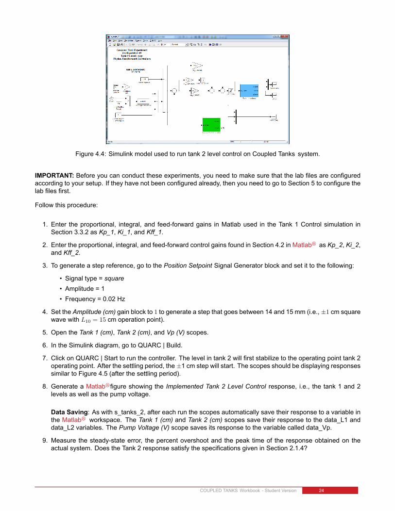
Figure 4.4: Simulink model used to run tank 2 level control on Coupled Tanks system.

IMPORTANT: Before you can conduct these experiments, you need to make sure that the lab files are configuredaccording to your setup. If they have not been configured already, then you need to go to Section 5 to configure thelab files first.


1. Enter the proportional, integral, and feed-forward gains in Matlab used in the Tank 1 Control simulation inSection 3.3.2 as Kp_1, Ki_1, and Kff_1.


3. To generate a step reference, go to the Position Setpoint Signal Generator block and set it to the following:


4. Set the Amplitude (cm) gain block to 1 to generate a step that goes between 14 and 15 mm (i.e., ±1 cm squarewave with L10 = 15 cm operation point).

5. Open the Tank 1 (cm), Tank 2 (cm), and Vp (V) scopes.

6. In the Simulink diagram, go to QUARC | Build.

7. Click on QUARC | Start to run the controller. The level in tank 2 will first stabilize to the operating point tank 2operating point. After the settling period, the±1 cm step will start. The scopes should be displaying responsessimilar to Figure 4.5 (after the settling period).

8. Generate a Matlabrfigure showing the Implemented Tank 2 Level Control response, i.e., the tank 1 and 2levels as well as the pump voltage.

Data Saving: As with s_tanks_2, after each run the scopes automatically save their response to a variable inthe Matlabr workspace. The Tank 1 (cm) and Tank 2 (cm) scopes save their response to the data_L1 anddata_L2 variables. The Pump Voltage (V) scope saves its response to the variable called data_Vp.

9. Measure the steady-state error, the percent overshoot and the peak time of the response obtained on theactual system. Does the Tank 2 response satisfy the specifications given in Section 2.1.4?


(a) Tank 1 Level (b) Tank 2 Level (c) Pump Voltage

Figure 4.5: Typical response when controlling tank 2 level.

4.4 Results

Fill out Table 4.1 with your answers from your control lab results - both simulation and implementation.

Description Symbol Value UnitsPre Lab QuestionsTank 1 Control GainsProportional Control Gain kp,1 V/cmIntegral Control Gain ki,1 V/(cm-s)Feed Forward Control Gain Kff,1 V/

√cm

Tank 2 Control GainsProportional Control Gain kp,2 cm/cmIntegral Control Gain ki,2 1/sFeed Forward Control Gain Kff,2 cm/cm

Tank 2 Control SimulationSteady-state error ess cmSettling time ts sPercent overshoot PO %

Tank 2 Control ImplementationSteady-state error ess cmSettling time ts sPercent overshoot PO %

Table 4.1: Tank 2 Level Control Results Results


5 SYSTEM REQUIREMENTSRequired Software

• Microsoft Visual Studio (MS VS)

• Matlabr with Simulinkr, Real-Time Workshop, and the Control System Toolbox

• QUARCr

See the QUARCr software compatibility chart in [3] to see what versions of MS VS and Matlab are compatible withyour version of QUARC and for what OS.

Required Hardware

• Data acquisition (DAQ) device that is compatible with QUARCr. This includes Quanser DAQ boards suchas Q2-USB, Q8-USB, QPID, and QPIDe and some National Instruments DAQ devices. For a full listing ofcompliant DAQ cards, see Reference [1].

• Quanser Coupled Tanks.

• Quanser VoltPAQ-X1 power amplifier, or equivalent.

Before Starting Lab

Before you begin this laboratory make sure:

• QUARCris installed on your PC, as described in [2].

• DAQ device has been successfully tested (e.g., using the test software in the Quick Start Guide or the QUARCAnalog Loopback Demo).

• Coupled Tanks and amplifier are connected to your DAQ board as described Reference [5].


5.1 Overview of Files

File Name DescriptionCoupled-Tanks User Manual.pdf This manual describes the hardware of the Coupled Tanks

system and explains how to setup and wire the system forthe experiments.

Coupled-TanksWorkbook (Student).pdf This laboratory guide contains pre-lab questions and labexperiments demonstrating how to design and imple-ment controllers for on the Coupled Tanks plant usingQUARCr.

setup_lab_tanks.m The main Matlab script that sets the Coupled Tanks con-trol and model parameters. Run this file only to setup thelaboratory.

config_coupled_tanks.m Returns the Coupled Tanks system parameters as well asthe amplifier limits VMAX_AMP and IMAX_AMP.

s_tanks_1.mdl Simulink file that simulates the Tank 1 Level Control, i.e.,Coupled Tanks Configuration #1 system.

s_tanks_2.mdl Simulink file that simulates the Tank 2 Level Control, i.e.,Coupled Tanks Configuration #2 system.

s_tanks_3.mdl Simulink file that simulates the Tank 2 Level Control whenthe Coupled Tanks is in Configuration #3. Note that thereare no instructions on how ot use any of the Configuration#3 files.

q_tanks_1.mdl Simulink file that implements the PI+FF controller on theCoupled Tanks system using QUARCr when setup inConfiguration #1.

q_tanks_2.mdl Simulink file that implements the PI+FF controller on theCoupled Tanks system using QUARCr when setup inConfiguration #2.

q_tanks_3.mdl Simulink file that implements the PI+FF controller on theCoupled Tanks system using QUARCr when setup inConfiguration #3. Note that there are no instructions onhow ot use any of the Configuration #3 files.

Table 5.1: Files supplied with the Coupled Tanks

5.2 Setup for Tanks 1 Control Simulation

Before beginning the in-lab procedure outlined in Section 3.3.2, the s_tanks_1 Simulink diagram and the setup_lab_tanks.mscript must be configured.

Follow these steps:

1. Load the Matlabr software.

2. Browse through theCurrent Directory window inMatlab and find the folder that contains the file setup_lab_tanks.m.

3. Open the setup_lab_tanks.m script.

4. Configure setup_lab_tanks.mscript: Make sure the script is setup to match your system configuration:

• K_AMP to 3 (unless your amplifier gain is different)• AMP_TYPE to your amplifier type (e.g., VoltPAQ).• CONTROLLER_TYPE to 'MANUAL'.


5. Run setup_lab_tanks.m to setup the Matlab workspace.

6. Enter the PI+FF control gains you found in the Pre-Lab Questions Section 3.2 in the Matlab as the variables:Kp_1, Ki_1, Kff_1.

7. Open the s_tanks_1.mdl Simulink diagram, shown in Figure 3.4.

5.3 Setup for Tanks 2 Control Simulation

Before beginning the in-lab procedure outlined in Section 4.3.2, the s_tanks_2 Simulink diagram and the setup_lab_tanks.mscript must be configured.

Follow these steps:

1. Go through the steps outlined in Section 5.2 to configure the setup_lab_tanks.m script properly.

2. Run setup_lab_tanks.m to setup the Matlab workspace.

3. Enter the proportional, integral, and feed-forward gains in Matlab used in the Tank 1 Control simulation inSection 3.3.2 as Kp_1, Ki_1, and Kff_1.


5. Open the s_tanks_2.mdl Simulink diagram, shown in Figure 4.2.

5.4 Setup for Implementing Tank 1 Control

Before performing the in-lab exercises in Section 3.3.3, the q_tanks_1 Simulink diagram and the setup_lab_tanks.mscript must be configured.

Follow these steps to get the system ready for this lab:

1. Go through the Coupled Tanks User Manual ([5]) to set up the system:

• Hardware set up and connections.• Make sure the pressure sensors of the system have been calibrated.• Set up the Coupled Tanks in Configuration #1 (i.e., tank 1 only).

2. If using the VoltPAQ-X1, make sure the Gain switch is set to 3.

3. Configure and run setup_lab_tanks.m as explained in Section 5.2.

4. Open the q_tanks_1.mdl Simulink diagram, shown in Figure 3.6.

5. Configure DAQ: Ensure the HIL Initialize block in the Simulink model is configured for the DAQ device that isinstalled in your system. See Reference [1] for more information on configuring the HIL Initialize block.

5.5 Setup for Implementing Tank 2 Level Control

Before performing the in-lab exercises in Section 4.3.3, the q_tanks_2 Simulink diagram and the setup_lab_tanks.mscript must be configured.

Follow these steps to get the system ready for this lab:


1. Go through the Coupled Tanks User Manual ([5]) to set up the system:

• Hardware set up and connections.• Make sure the pressure sensors of the system have been calibrated.• Set up the Coupled Tanks in Configuration #2 (i.e., tank 1 feeds into tank 2).

2. If using the VoltPAQ-X1, make sure the Gain switch is set to 3.

3. Configure and run setup_lab_tanks.m as explained in Section 5.2.

4. Open the q_tanks_2.mdl Simulink diagram, shown in Figure 4.4.

5. Configure DAQ: Ensure the HIL Initialize block in the Simulink model is configured for the DAQ device that isinstalled in your system. See Reference [1] for more information on configuring the HIL Initialize block.


6 LAB REPORTThis laboratory contains two groups of experiments, namely,

1. Tank 1 Level control, and

2. Tank 2 Level control.

For each experiment, follow the outline corresponding to that experiment to build the content of your report. Also,in Section 6.3 you can find some basic tips for the format of your report.

6.1 Template for Tank 1 Level Control Report

I. PROCEDURE

1. Simulation

• Briefly describe the main goal of the simulation.• Briefly describe the simulation procedure in Step 7 in Section 3.3.2.

2. Implementation

• Briefly describe the main goal of this experiment.• Briefly describe the experimental procedure in Step 8 in Section 3.3.3.

II. RESULTSDo not interpret or analyze the data in this section. Just provide the results.

1. Response plot from step 7 in Section 3.3.2, Tank1 level control simulation.

2. Response plot from step 8 in Section 3.3.3, Tank 1 level control implementation.

3. Provide applicable data collected in this laboratory (from Table 3.1).

III. ANALYSISProvide details of your calculations (methods used) for analysis for each of the following:

1. Peak time, percent overshoot, steady-state error, and input voltage in Step 8 in Section 3.3.2.


IV. CONCLUSIONSInterpret your results to arrive at logical conclusions for the following:

1. Whether the controller meets the specifications in Step 8 in Section 3.3.2, Tank1 level control simulation.

2. Whether the controller meets the specifications in Step 9 in Section 3.3.3, Tank1 level control implementation.


6.2 Template for Tank 2 Level Control Report

I. PROCEDURE

1. Simulation

• Briefly describe the main goal of the simulation.• Briefly describe the simulation procedure in Step 7 in Section 4.3.2.

2. Implementation

• Briefly describe the main goal of this experiment.• Briefly describe the experimental procedure in Step 8 in Section 4.3.3.

II. RESULTSDo not interpret or analyze the data in this section. Just provide the results.

1. Response plot from step 7 in Section 4.3.2, Tank2 level control simulation.

2. Response plot from step 8 in Section 4.3.3, Tank2 level control implementation.

3. Provide applicable data collected in this laboratory (from Table 4.1).

III. ANALYSISProvide details of your calculations (methods used) for analysis for each of the following:



IV. CONCLUSIONSInterpret your results to arrive at logical conclusions for the following:

1. Whether the controller meets the specifications in Step 9 in Section 4.3.3, Tank2 level control implementation.


6.3 Tips for Report Format

PROFESSIONAL APPEARANCE

• Has cover page with all necessary details (title, course, student name(s), etc.)

• Each of the required sections is completed (Procedure, Results, Analysis and Conclusions).

• Typed.

• All grammar/spelling correct.

• Report layout is neat.

• Does not exceed specified maximum page limit, if any.

• Pages are numbered.

• Equations are consecutively numbered.

• Figures are numbered, axes have labels, each figure has a descriptive caption.

• Tables are numbered, they include labels, each table has a descriptive caption.

• Data are presented in a useful format (graphs, numerical, table, charts, diagrams).

• No hand drawn sketches/diagrams.

• References are cited using correct format.


REFERENCES[1] Quanser Inc. QUARC User Manual.

[2] Quanser Inc. QUARC Installation Guide, 2009.

[3] Quanser Inc. QUARC Compatibility Table, 2010.

[4] Quanser Inc. Coupled Tank User Manual, 2012.


Solutions for teaching and research. Made in Canada.

[email protected] +1-905-940-3575 QUANSER.COM

Magnetic LevitationCoupled Tanks

Process control plants for teaching and research

These plants are ideal for intermediate level teaching. They are also suitable for research relating to traditional or modern control applications of process control. For more information please contact [email protected]

©2013 Quanser Inc. All rights reserved.

Documents

Coupled Tanks Experiment for MATLAB /Simulink Users