Embed Size (px)
Citation preview
NASA Contractor Report 189150 /.79
Coupled Structural/Thermal/Electromagnetic
Analysis/Tailoring of Graded
Composite StructuresFirst Annual Status Report
R.L. McKnight, P.C. Chen, L.T. Dame, H. Huang,
and M. Hartle
General Electric
Cincinnati, Ohio(NASA-CR-I89150) COUPLED
STRUCTURALITHERMAL/ELECTROMAGNETICANALYSIS/TAILORING OF GRADED
COMPOSITF STRUCTURES Annual Status
Rnport No. I (GE) 99 p
G3139
N93-13443
Uncl_s
0131796
April 1992
Prepared forLewis Research Center
Under Contract NAS3-24538
N/ ANational Aoronaulics and
Spaco Adminislration
https://ntrs.nasa.gov/search.jsp?R=19930004255 2019-08-10T20:23:31+00:00Z

!
J
jr

FOREWORD
This report has been prepared to expedite early domestic dissemination
of the information generated under the contract. The data and conclusions
must be considered preliminary and subject to change as further progress is
made on this program. This is a progress report covering the work done
during the first 12 months of the contract; it is not a final report.
The NASA Program Manager is Dr. C.C. Chamis.
ABSTRACT
Accomplishments are described for the first year effort of a 5-year pro-
gram to develop a methodology for coupled structural/thermal/electromagnetic
analysis/tailoring of graded composite structures. These accomplishments
include: (I) the results of the selective literature survey; (2) 8-, 16-, and
20-noded isoparametric plate and shell elements; (3) large deformation struc-
tural analysis; (4) Eigenanalysis; (5) anisotropic heat transfer analysis; and
(6) anisotropic electromagnetic analysis.


TABLE OF CONTENTS
Section
1.0
2.0
APPENDIX A
APPENDIX B
APPENDIX C
INTRODUCTION
I.I Executive Summary
TECHNICAL PROGRESS
2.1 Task I - Selective Literature Survey
2.2 Task II - Graded Material Finite Elements
2.2.1 Task IIA - Plate Elements
2.2.2 Task liB - Shell Elements
2.2.3 Task IIC - Graded Composite Materials
2.2.4 Task liD - I/0 and Solution Techniques
2.2.5 Task liE - Stand-Alone Codes
Accumulated Literature
Closed-Form Eigenvalue Solutions
Eigenshift and Rayleigh Quotient Example
i
3
i0
I0
i0
i0
i0
67
74
77
79
91
93
f111
P t
PRECEDING PAGE BLANK NOT FILMED

I.
2.
3.
4.
5.
6.
7.
8.
9.
I0.
Ii.
12.
13.
LIST OF ILLUSTRATIONS
Program Flow Chart.
Composite Analysis System.
Total Composite Analysis System.
CSTEH System.
Constitutive Model - Structural Model Interaction.
Typical Two'Dimensional Eiement_
Eight-Noded Solid Coordinate and Node Numbering System.
Sixteen-Noded Solid Coordinate and Node Numbering System.
Twenty-Noded Isoparametric Finite Element Mapping.
Twenty-Noded Isoparametric Finite Element Mapping.
Patch Test for Solids.
Straight Cantilever Beam.
Curved Beam.
2
4
5
6
7
. 13
16
19
23
24
68
69
70
_v

LIST OF TABLES
Table
I •
2.
3.
4.
5.
6.
7.
Nodal Coordinates for 20-Nodal Element.
Gauss-Legendre Quadrature.
Newton-Cotes Quadrature.
Existing FEM Code.
CSTEM Stiffness Code.
Theoretical Solutions.
Twenty-Noded Bricks.
25
32
33
71
72
73
75
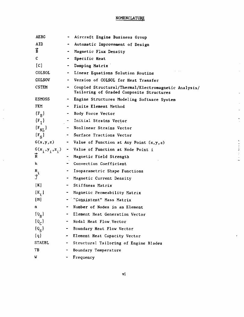
NOMENCLATURE
AEBG
AID
C
[cl
COLSOL
COLSOV
CSTEM
ESMOSS
FEM
{rB }
{FI }
{FNL}
{FS }
G(x,y,z)
G(xl,Yi,Z i)
g
h
H.1
J
[El
[Ktl[MI
n
{QB}
{ec }
{Qs}
STAEBL
TB
W
- Aircraft Engine Business Group
- Automatic Improvement of Design
- Magnetic Flux Density
- Specific Heat
- Damping Matrix
- Linear Equations Solution Routine ..........
- Version of COLSOL for Heat Transfer
- Coupled Structural/Thermal/Electromagnetic Analysis/
Tailoring of Graded Composite Structures
- Engine Structures Modeling Software System
- Finite Element Method
- Body Force Vector
- Initial Strains Vector
- Nonlinear Strains Vector
- Surface Tractions Vector
- Value of Function at Any Point (x,y,z)
- Value of Function at Node Point i
- Magnetic Field Strength
- Convection Coefficient
- Isoparametric Shape Functions
- Magnetic Current Density
- Stiffness Matrix
- Magnetic Permeability Matrix
- -"Consistent" Mass Matrix
Number of Nodes in an Element
Element Heat Generation Vector
Nodal Heat Flow. Vector
Boundary Heat Flow Vector
Element Heat Capacity Vector
Structural Tailoring of Engine Blades
Boundary Temperature
Frequency
m
w
vi

NOMENCLATURE (Concluded)
¥
I
P
- Surface Heat Transfer Coefficient
- Reciprocal Permeability
- ith Eigenvalue
- Magnetic Permeability
- Resistivity
- ith Eigenvector
vii


1.0 INTRODUCTION
This technical program is the work of the Engineering Mechanics and Life
Management Section of the Aircraft Engine Business Group (AEBG) of the General
Electric Company in response to NASA RFP 3-537260, "Coupled Structural/
Thermal/Electromagnetic (CSTEM) Analysis/Tailoring of Graded Composite Struc-
tures." The overall objective of this program is to develop and verify analy-
sis and tailoring capability for graded composite engine structures taking
into account the coupling constraints imposed by mechanical, thermal, acous-
tic, and electromagnetic loadings.
The first problem that will be attacked is the development of plate and
shell finite elements capable of accurately simulating the structural/thermal/
electromagnetic response of graded composite engine structures. Because of
the wide diversity of engine structures and the magnitudes of the imposed
loadings, the analysis of these is very difficult and demanding when they are
composed of isotropic, homogeneous materials. The added complexity of direc-
tional properties which can vary significantly through the thickness of the
structure will challenge the state-of-the-art in finite element analysis. We
are applying AEBG's 25 years of experience in developing and using structural
analysis codes and the exceptional expertise of our University consultants
toward the successful conclusion of this problem. To assist _,_ this, we are
drawing heavily on previously funded NASA programs.
We are drawing on NASA programs NAS3-23698, 3D Inelastic Analysis Methods
For Hot Section Components, and NAS3-23687, Component Specific Modeling, in
our development work on the plate and shell elements. In addition to these
two programs, we will draw on NAS3-22767, Engine Structures Modeling Software
System (ESMOSS), and NAS3-23272, Burner Liner Thermal/Structural Load Model-
ing, in Task III when we generate a total CSTEM Analysis System around these
finite elements. This will guarantee that we are using t_e latest computer
software technology and will produce an economical, flexible, easy to use
system.
In our development of a CSTEM tailoring system, we will build on NASA
Program NAS3-22525, Structural Tailoring of Engine Blades (STAEBL) and AEBG
program, Automatic Improvement of Design (AID), in addition to the program
system philosophy of ESMOSS. Because of the large number of significant
parameters and design constraints, this tailoring system will be invaluable
in promoting the use of graded composite structures.
All during this program, we will avail ourselves of the experience and
advice of our Low Observables Technology group. This will be particularly
true in the Task V proof-of-concept. Their input will be used to assure the
relevancy of the total program.
Figure 1 shows our program and major contributions in flowchart form.
This gives a visual presentation to the synergism that will exist between
this program and other activities.

TexasA&M
NAS3-236983D Inelastic
NAS3-22767ESMOSS
NAS3-22525
STAEBL
Task ISelectiveLiterature
Survey
Task IIGradedMaterial
FiniteElements
Task IIICSTEM
Analyzer
Task IVCSTEM
Tailoring
Task V
CSTEM Tailoringof Simulated
Components
NAS3-23687
ComponentSpecific
Modeling
Texas IA&M
NAS3-23272BurnerLiner
AEBGAutomatic
Improvementof Design
(AID)
AEBGLow
Observable
Technology Task VI
Reporting @ NASA ProgramManager's Approval
Figure i. Program Flow Chart.
2

Figure 2 depicts an integrated analysis of composite structures currently
under development in the composite users' community. The severe limitations
of such a system are not highlighted because three major steps in the process
are not shown. Figure 3 adds these steps. The analysis system really begins
with a definition of geometry. A user then defines a finite element model
simulating this geometry and the anticipated loading. The process then moves
to defined Step 3. One cycle through the process ends with the prediction of
individual ply average stresses and strains. Now comes a significant produc-
tivity drain, namely, manual intervention to evaluate these stresses and
strains against strength and durability limits. Based on this, the user must
decide to (I) change the finite element model, (2) change the composite lami-
nate, (3) both of the above, or (4) stop here.
Obviously, there is a considerable cost savings to be obtained by select-
ing Number 4. The CSTEM system will obviate the reasons for selecting Number
4. This system, shown in Figure 4, begins with the definition of geometry, as
before, but then proceeds to a definition of master regions Which contain all
of the necessary information about geometry, loading, and material properties.
Step 3 is a constitutive model which develops the necessary structurai, ther-
mal, and electromagnetic properties based on a micromechanics approach. Fur-
thermore, this constitutive model will contain the logic to generate the
global finite element model based on the variation of the properties, as
depicted in Figure 5. Using a nonlinear incremental technique, these global
models will be solved for their structural, thermal, and electromagnetic
response. Based on this response the global characteristics will be evalu-
ated, with convergence criteria and decisions made on remodeling. Once the
global characteristics meet the accuracy requirements, the local characteris-
tics are interrogated and decisions made on remodeling because of strength,
durability, or hereditary effects. Once this cycle has been c+abilized, opti-
mization will be performed based on design constraint. Our goal in Task II is
to develop finite elements whose characteristics make this system possible.
Although the structural properties have been highlighted, the thermal and
electromagnetic properties have as much or more variation, and less work has
been done in these areas.
I. 1 EXECUTIVE SUMMARY
Meetings were held with designers and management of the Low Observables
Sections to determine their requirements. It was learned that the generic
problem was that structures designed for optimum electromagnetic capabilities
often have nonoptimum thermal and structural capabilities. There is a need
for a tool that can accurately and efficiently analyze and iterate among
these three fields so that viable compromise designs can be generated. At
present, no such tool exists.
Based on the Statement of Work and the results of the literature survey,
we have established the 8-, 16-, and 20-noded isoparametric finite elements
to be used to develop the CSTEM plate and shell element capabilities. These
three elements meet the requirements for the plate elements. They have
quadrilateral planform and are reducible to triangular planform, have nodes
on the upper and lower surfaces, will meet accuracy requirements, and have

4
0J _J ,-4
_'_ _ O•H I-,
I-4
¢1
•H ,._
,-4 l-J _
1..1
_--I
14 O _ m
•_ 0
4.J
I..-I
.I.I
0r_
°_,.t

01
01
01
°_
0
0
0
e_
0
o,-.I

I4-)(J
CrJ
Q;&J
°io_rO
°i°_
°I<
Q;4-)
0
0 m
6

(J
i.J@
0_3
0
0
4-)@
4n
0:_ CO
0
O_
-,-I
0O_
0ED
OJ
0(J
C) () C) C) ¢
)
]O []O ODD0[
(
)0 000 O O0 [
0
0
0
7 o0
O
0
(Jr_W@
@
m
!
,-t
1-1(8
o
oel
7

the proper degrees of freedom to perform all three types of analyses. The
16- and 20-noded elements meet all of the requirements for the shell elements,
including double curvature.
Having established the basic building block, progress has been made in
the three major areas, that is, structural, thermal, and electromagnetic,
while maintaining the maximum commonality in computer software, such as shape
functions, Jacobians, et cetera.
Progress has occurred in the structural analysis area, as follows:
Defined the nonlinear equilibrium system of equations, including
large deformation effects. Established an incremental, updated
Lagranian solution.
Defined the overall programming architecture.
Wrote the modular stiffness matrix subroutines.
Wrote the modular mass matrix subroutines.
Wrote the subroutines for modular load.
Wrote subroutines for modular assembly and boundary conditions.
Established the input data format and wrote input subroutines.
Wrote the modular eigenvalue/eigenvector routines.
Incorporated the linear constraint equations.
Wrote a stress smoothing subroutine.
Wrote a modular equation solver.
Studied the micromechanics approach to stiffness formulation for
composite elements.
Ran the verification and validation cases for the elasticity and
eigenanalysis capabilities.
The file structure and data flow are currently under development.
In the thermal area, the following progress has been made:
Anisotropic heat transfer equations have been defined for both
linear and nonlinear conductivities and for steady-state and
transient problems.
All of the subroutines necessary to perform a linear, steady-state,
anisotropic heat transfer problem have been written, making maximum
use of the code that is common with the structural analysis.
In the electromagnetic area, the following progress has been made.
• Results of the literature survey have been studied.

Dr. M.V.K. Chari, General Electric's expert on finite element elec-
trical analysis, has been contacted.
Finite element equations for the electromagnetic field problem have
been established.

2.0 TECHNICAL PROGRESS
2.1 TASK I - SELECTIVE LITERATURE SURVEY
The first activity on this program was to perform'a selective literature
search using our internal General Electric data bases, the external COMPENDEX
data base, and the literature supplied by the Texas A&M consultants. The
pertinent articles turned up by this search are enumerated in Appendix A.
Based on the results of this survey, it was proposed to the NASA Program
Manager that the family of 8-, 16-, and 20-noded isoparametric elements be
used for all three aspects of this program: structural, thermal, and electro-
magnetic.
The proposed plan of attack was:
Work on three parallel efforts - structural, heat transfer, and
electromagnetic
Use an incremental updated Lagrangian approach for the large dis-
placement structural problem.
• Handle the coupling among the fields by an iterative procedure.
2.2 TASK II - GRADED MATERIAL FINITE ELEMENTS
2.2.1 Task IIA - Plate Elements
The 8-, 16-, and 20-noded isoparametrics will be used as plate elements
and shell elements. As plate elements, there will be a restriction that the
midsurfaces be in a plane. This restriction will be the only difference
between the plate and shell elements and, primarily, affects the program
input. A simpler geometric and loading input can be used. Beyond this, all
of the technical requirements are the same as for the shell elements. These
will be discussed in the next section.
2.2.2 Task liB - Shell Elements
AEBG has developed and used many different plate and shell elements.
The elements to be used in this program are the 8-, 16-, and 20-noded iso-
parametric elements. These have been used both as plates and as doubly curved
shells for both linear and nonlinear material behavior. A review of these
elements follows.
Isoparametric Solid Elements
The isoparametric solid elements permit the modeling of any general
three-dimensional (3D) object, since the elements represent a discretization
IO

of the object into finite elements which are 3D continuous representations.The basic term "isoparametric" meansthat the elements utilize the same inter-polating functions (also called "shape functions") to interpolate geometry,displacements, strains, and temperatures. It is, therefore, important that
the user be aware that not just any displacement, geometry, and temperature
field to be analyzed is necessarily compatible with a given element mesh.
This is particularly true where high temperature or strain gradients occur.
The following sections discuss the basic element formulation assumptions.
Shape functions are used to describe the variation of some function G
within an element in terms of the nodal point values.
n
G(x,y,z) = _ HiGi(xi,Yi,Z i)
i=l
whe re
G(x,y,z) = the value of the function (such as displacement, tempera-
ture) at any point with coordinates (x,y,z) within an
element
G (xi,Yi,z i) = the value of the function at node point i
H.
1= the element "shape function" associated with node i
n = the number of nodes describing intraelement variation.
In order to ensure monotonic convergence to the correct results, shape
functions must satisfy several requirements. Satisfaction of these require-
ments results in convergence from an upper bound. These displacement function
requirements are:
They must include all possible rigid body displacements
They must be able to represent constant strain states
They must be differentiable within elements and compatible between
adjacent elements.
While the above conditions prove valuable for establishing upper bounds
for solutions, they are not essential. Incompatible displacement modes are
widely and successfully used. Their principal disadvantage is that stiffness
may no longer be bounded from above.
Curvilinear coordinates are introduced into the isoparametric concept to
overcome the difficulty of formulating shape functions in global Cartesian
coordinates. Also, generality in element geometry definition is obtained by
this process.
ii

A local curvilinear coordinate system (r,s,t), which ranges from -1 to
I within each element, is_introduced in which shape functions are formulated.
Also, a mapping from curvilinear to global coordinates is defined. A typical
two dimensional element is shown in Figure 6.
The same polynomial terms used in the Cartesian coordinates are used but
with the curvilinear coordinates r,s,t replacing x, y, and z to generate
shape functions. The r, s, and t coordinates are the same for all global
element configurations.
Typical finite element equilibrium equations:
I. Structural
[M]{_i} + [C]{dl} + [Z]{u i} = {FB} + {F s} + {F I} + {F C} + {FNL}
[M] = SvP[H]T[H]dv "Consistent" mass matrix
[C] = Damping matrix
[K] = Iv[B]T[D][B]dv Stiffness matrix
{FB} = /v[H]T{fB}dV Body forces
{Fs} = $s[HS] T {fs}dS Surface tractions
{FI} = Iv[B]T[D]{¢T}dV Initial strains
{FNL } = Iv[B]T[D]{¢NL}dv Nonlinear strains
where
{ui}T = [uI v I w I u 2 v 2 w2 .... ]
{u}Z = [u v w]
{u} = [H]{ui}
{¢} = [B]{ui}
12

P84-73-2
4
r = -1
8
ss =+I
7
01 5 2
S = -1
3
r = +l
6
r
(a) Curvilinear Coordinates
Y
8
1
r X
(b) Global Coordinates
Figure 6. Typical Two-Dimensional
Element.
13

{a} - [D]{¢ e) - [D] ({eTOT}-{gTHERM}-(eNL})
,
{fB} T = [fBx fBy fBz]
(fS} T = [fSx fSy fsz]
Thermal
[q]{Ti) + [K]{Ti} " {QB) + {Qs} + {Qc}
[q] = Yv c[H]T[H]dv Element heat capacity
[K] = Iv[B]T[R][B]dv + IS2S [HS]T[HS]dS2
Element conductivity
[QB] = Iv[H]T{qB}dV Element heat generation
[Qs ] " /Sl[lIS1]T{qs}dSl + IS a[HS]TTBdS2
Boundary heat flow
(Qc } = Concentrated heat flow
where
{Ti) T = iT1 T2 T3...]
{T) - [H] {T i}
{q} - [B]{T i}
C
TB
= Specific heat
ffiBoundary temperature
= Surface heat transfer coefficient
14

3. Electromagnetic
y[S]{A i} + _[D] (A i} + _[E]{A i} + J_._w[T]{A i} = [T]iJi}0
where iS], [D], [E], and iT] are functions of [H].
{A i} = Nodal point values of potential
{Ji} = Nodal point values of forcing functions
= Reciprocal permeability
w = Frequency
o = Resistivity
Other field problems have similar finite element expressions.
8-Noded Solid
The 8-noded solid element utilizes a formal mapping technique with dis-
placement functions defined by a series of interpolating polynomials called
"shape functions." In this manner, an arbitrary solid of six faces can be
mapped from a parent coordinate system as shown in Figure 7. The numbering
sequence must be as shown in this figure, except the user may define the nodes
NI and N5 as any convenient nodes on the solid. Note that node N1 has the
parent coordinates (r,s,t) = (1,1,1). Once this has been established by the
user, all face definition given later in this section is established.
The shape functions for this element are as follows:
H 1 = (I + r) (1 + s) (I + t)/8
H2 = (I - r) (I + s) (I + t)/8
H3 = (I - r) (I - s) (I + t)/8
H4 = (I + r) (I - s) (I + t)/8
H5 = (I + r) (1 + s) (1 - t)/8
H6 = (I - r) (I + s) (I - t)/8
H7 = (i - r) (I - s) (I - t)/8
H8 = (I + r) (I - s) (I - t)18
Since this element has linear displacements on an edge, the ability to model
the deformation due to bending is not possible, and the element will be overly
stiff in bending. To overcome this, the addition of non-nodal degrees of
freedom can be used as an option. These are called "incompatible modes," and
are condensed out of the element stiffness after stiffness generation, leaving
24 degrees of freedom per element. The interpolation for all element proper-
ties and displacements is given by: 15

P84-73-3
S
Parent Coordinate System
/
(a) Element Mapping
t
N3 A
N _ .....
t
Mapped Element
(Physical Space)
N2
./r
s
(b) Node-Numbering :gystem ...............
Figure 7. Eight-Noded Solid Coordinate and Node Numbering System.
16
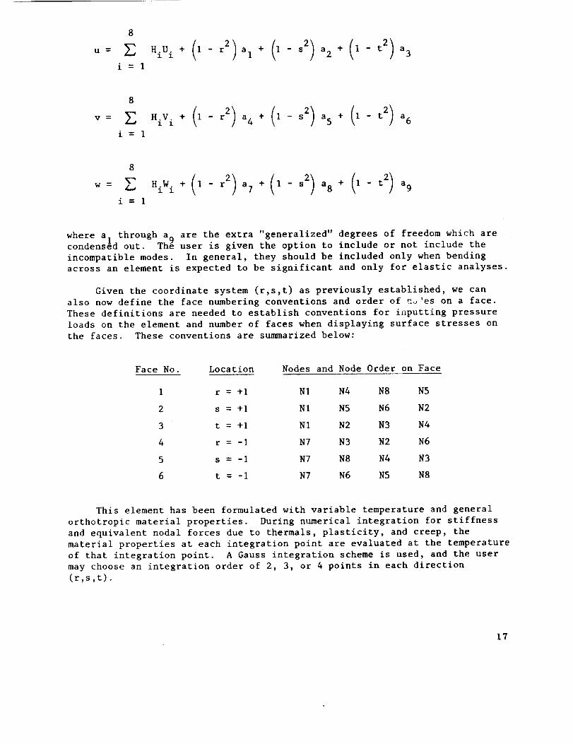
U
i = 1
V _
i= 1
W _
8
Z_.,
i= 1
Hiwi+(i_r2)a,+_s2)as (1-t2)a9
where a. through a^ are the extra "generalized" degrees of freedom which are
condensed out. The user is given the option to include or not include the
incompatible modes. In general, they should be included only when bending
across an element is expected to be significant and only for elastic analyses.
Given the coordinate system (r,s,t) as previously established, we can
also now define the face numbering conventions and order of n_es on a face.
These definitions are needed to establish conventions for inputting pressure
loads on the element and number of faces when displaying surface stresses on
the faces. These conventions are summarized below:
Face No. Location Nodes and Node Order on Face
I r = +I N1 N4 N8 N5
2 s = +I N1 N5 N6 N2
3 t = +I N1 N2 N3 N4
4 r = -I N7 N3 N2 N6
5 s = -I N7 N8 N4 N3
6 t = =I N7 N6 N5 N8
This element has been formulated with variable temperature and general
orthotropic material properties. During numerical integration for stiffness
and equivalent nodal forces due to thermals, plasticity, and creep, the
material properties at each integration point are evaluated at the temperature
of that integration point. A Gauss integration scheme is used, and the user
may choose an integration order of 2, 3, or 4 points in each direction
(r,s,t).
17

16-Noded Solid
The 16-noded solid follows the same type of development for stiffness
and loads as the 8-noded solid and, like the 8-noded solid, it has three dis-
placement degrees of freedom per node, thus a total of 48 degrees of freedom
on the element. Since this element has higher order interpolating functions
in two directions on an edge, this element is sometimes called a "thick shell"
element, as it can be used with reasonable approximation in this type of
analysis where the shell thickness is in the t direction.
The node numbering sequence must be as shown in Figure 8, except that
the user can define the location of Nodes N 1 and N as desired. Note that
Node N I has the parent coordinates (r,s,t) = (I,I,_). Since this has beenestabllshed, all face numbering is then defined.
Starting with the basic interpolating functions for the corners, wedefine:
G1 = (I + r) (1 + s) (1 + t)/8
G3 = (I - r) (1 + s) (1 + t)/8
G5 = (I - r) (I - s) (I + t)18
G7 = (1 + r) (I - s) (I + t)/8
G9 = (I + ri(1 + s) (I - t)18
GI] = (] - r) (I + s) (I - t)18
G13 = (1 - r) (1 - s) (1 - t)18
GI5 = (1 + r) (1 - s) (I - t)/8
Then, for the midside nodes, the shape functions are:
H 2 = (I - r) (I + s) (1 + t)14
H 4 = (I - r) (I - s) (I + t)14
H6 = (1 - r) (1 - s) (1 + t)/4
H8 = (1 + r) (1 - s) (1 + t)/4
H10 = (1 - r) (1 + s) (I - t)/4
H!2 = (I - r) (I - s) (I - t)14
HI4 = (1 - r) (1 - s) (1 - t)14
H16 = (I + r) (1 - s) (1 - t)14
18

P84-73-4
N15q
t
N5
N6
N3
Figure 8. Sixteen-Noded Solid Coordinate and
Node Numbering System.
19

and for the corner nodes, the modified shape functions are:
H 1 = G 1 - (H2 + H8)12
H 3 = G3 - (H2 + H4)12
H5 = G5 = (H4 + H6)/2
H7 = G7 - (H 6 + H8)/2
H9 = G9 - (HI0 + H16)/2
H11 = Gll (H10- + H12)/2
H13 = G13 - (H12 + H14)/2
H15 = G15 - (H14 + H16)12
As in the case of the 8-noded solid, the user may use an option to
specify that certain extra generalized degrees of freedom be added to intro-
duce "incompatible modes" for bending. If through-thickness bending in the t
direction is significant, these modes will prevent the element from being
overly stiff, These generalized degrees of freedom are condensed out after
stiffness formulation, leaving only the 48 nodal degrees of freedom. The
complete element interpolating functions, used to interpolate displacements,
etc., are thus:
--L-
[-
16 6
u = _ H.U. + _ _.a.1 1 1 1
i= 1 i= 1
20
16 6
V = Z H.V. + Z H,b,1 I 1 1
i= 1 i= 1

• 16 6
i i i i
i=l i=l
where the interpolating function coefficients for the generalized displace-
ments are:
HI = r (I - r 2) H2 = s (I - s 2) H3 = (I - t2)
H4 = rs (I - r 2) H5 = rs (i - s 2) R6 = (] - r2) (I - s 2)
and the variables a_ to a6, b I to b6, and c_ to c_ are the 18 generalizeddisplacements which I 1 bare condensed out after stiffness formulation.
Given the coordinate system (r,s,t) as previously established, we can
also now define the face numbering conventions and order of nodes on a face.
These definitions are needed to estab!ish conventions for inputting pressure
levels on the element and numbering of faces when displaying surface stresses
on the faces. These conventions are summarized below:
Face No. Location Nodes and Node Order on Face
1 r = +I N1 N8 N7 NI5 NI6 N_
2 s = +l N1 N9 NIO NIl N3 N2
3 t = +I NI3 N2 N3 N4 N5 N6
4 r = -I NI3 N4 N4 N3 Nil NI2
5 s = -I NI3 NI4 NI5 N7 N6 N5
6 t = -I NI3 NI2 NIl NIO N9 NI6
N7 N8
NI5 NI4
This element has been formulated with variable temperature general ortho-
tropic material properties. During numerical integration for stiffness and
equivalent nodal forces due to thermals, plasticity, and creep, the material
properties at each integration point are evaluated at the temperature of that
integration point. A Gauss integration scheme is used, and the user may
choose an integration order of 2, 3, or 4 points in each direction (r,s,t).
21
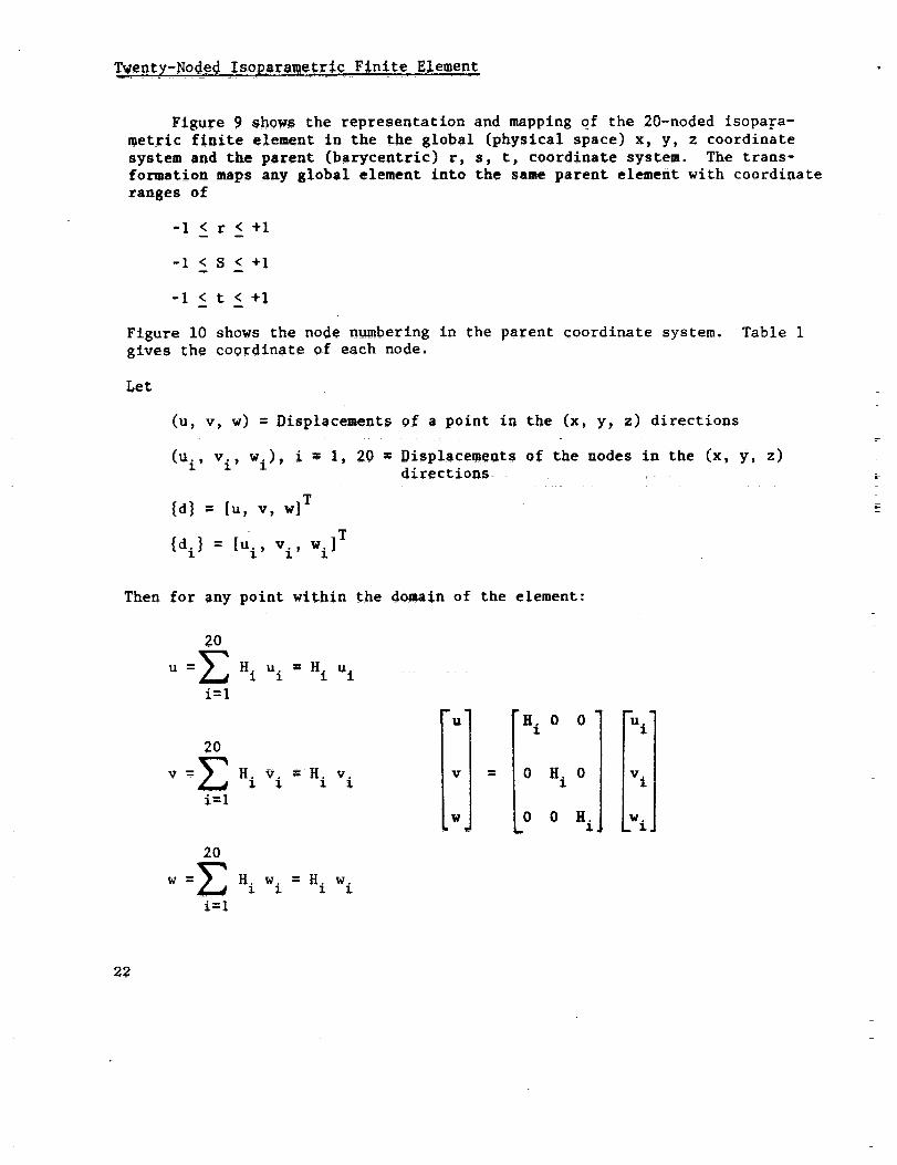
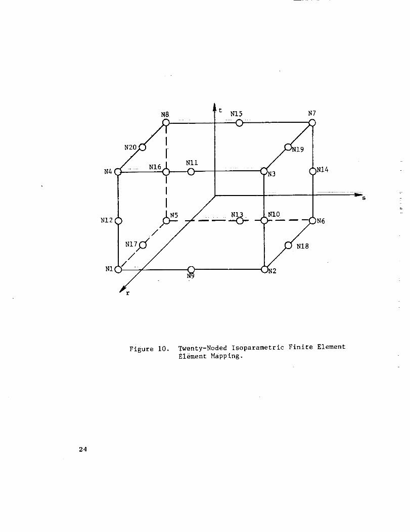
_e_ty-Nod_ed lsop.ar_etric Finite Element
Figure 9 shows the representation and mapping of the 20-noded isopa_a-
metric finite element in the the global (physical space) x, y, z coordinate
system and the parent (barycentric) r, s, t, coordinate system. The trans-
formation maps any global element into the same parent element with coordinate
ranges of
-! <r<+l
-i <S<+1
-I <t<+l
Figure i0 shows the node numbering in the parent coordinate system. Table I
gives the coordinate of each node.
Let
(u, v, w) = Displacements of a point in the (x, y, z) directions
(ui, vi, wi) , i = I, 20 = Displacements of the nodes in the (x, y, z)directions
{d} = [u, v, w] T
{di} = [ui, v i, wi]T
Then for any point within the domain of the element:
20
u =E Hi
i=l
u i = H i u i
20
v =E Hi v. = H. v.1 i i
i=l
2O
i=!H. wi=H. w.
I
vl:I
.wJ
H. 0 01
0 H. 0I
0 0 H.I
l •
U.I
v i
W,
22

x
\\ o
/
0
0
(x7,Y7,Z7,)
(-i, -i,-i)
(
() pJ
i
/I I
#/
O
O
O
t
s
(
r
(
(
(+i,+i,+i)
Figure 9. Twenty-Noded Isoparametric Finite Element
Mapping. 23
N4(
NI2(
NI(
N8
....... NI6_ Il
l
tNI5 N7
_3 ()N14
• r 5
NI0)N6
Figure I0o Twenty-Noded Isoparametrlc Finite Element
Element Mapping.
24

Table I. Nodal Coordinates for20-Nodal Element.
NodeNumb e r r__ s
1 1 -1
2 1 1
3 1 1
4 I -I
5 -I -I
6 -I 1
7 -I I
8 -1 -1
9 1 0
10 1 1
11 1 0
12 1 -1
13 -I 0
14 -1 1
15 -I 0
16 -1 -1
17 0 -1
18 0 1
19 0 1
20 0 -I
t
-I
-I
1
1
-I
-I
1
1
-I
0
1
0
-I
0
1
0
-I
-I
1
1
25

where the H i in terms of the parent coordinate system are given as follows.The basic corner noded shape functions are
G 1 = (1+r)(1-s)(1-t)/8
G2 = (l+r)(l+s)(l-t)/8
G3 = (l+r)(l+s)(l+t)/8
G4 = (l+r)(l-s)(l+t)/8
G5 = (l-r)(1-s)(1-t)/8
G6 = (l-r)(l+s)(1-t)/8
G7 = (1-r)(1+s)(z+t)/8
G8 = (1-r)(l-s)(1+t)/8
The midside node shape functions are
H 9 = (l+r)(l-s2)(l-t)/4
HI0 = (l+r)(1+s)(1-t2)/4
HI1 = (l+r)(1-s2)(1+t)/4
H12 = (l+r)(1-s)(1-t2)/4
HI3 = (l-r)(l-s2)(l-t)/4
HI4 = (l-r)(l+s)(l-t2)/4
H15 = (1-r)(l-s2)(l+t)/4
HI6 = (l-r)(l-s)(l-t2)/4
HI7 = (1-r2)(l-s)(l-t)/4
HI8 = (l-r2)(1+s)(1-t)/4
= (l-r2)(1+s)(1+t)/4H19
H20 = (l-r2)(l-s)(1+t)/4
The modified corner node shape functions are
H I = G 1 - (H9+HI2+H17)/2
H 2 = G2 - (H9+H10+HI8)/2
26

and
H3 = G3 - (HI0+HII+HI9)/2
H4 = G4 - (HII+HI2+H20)/2
H 5 = G5 - (HI3+HI6+HIT)/2
H6 = G6 - (H13+HI4÷H18)/2
H7 = G7 - (HI4+H15+HI9)/2
H8 = G8 - (HI5+H16+H20)/2
In a three-dimensional context_ the relations between the displacements
the strains are given by the following.
Six Strain-Displacement Relations
_U
xx _x
_V
yy Oy
_W-- m6
zz _z
exy = _ Yxy = _ +
gyz =
ZX
Yy_.= _ _ +
I 1(aw au)
Therefore, the strain at any point within the elements domain is given
by the following.
27

E x
_y
gZ
YxY I =
II
I
¥yzl
8u8x
8v8y
8w8z
8u 8v
8v _w
8w 8u
w
b
_H_i8x
8H.l
8y
0
8H.
8z
0
8H.l
8x
8H.i
8z
0
0
8H.I
8z
8H.i
8y
8H.
8x
U.
1
V°
1
I
wi
or
{_} = [Bi] {di}
g=B.d,1 1
Since the Hi are defined in the parent coordinate system, we need to define
the derivatives with respect to the global coordinate system by the chain
rule of differentiation.
8H 8H. 8H.8Hi i 8r I 8s I 8t
8x 8r 8x 8s 8x 8t 8x
0Hi 8Hi 8r 8H. 8HI 8s i 8t
8y Or 8y 8s 8y 8t 8y
8H i 8H. 8H. 8Hi 8r m 8s i 8t
8z 8r 8z 8s 8z 8t 8z
To produce the required terms for the above expressions we need to develop
the Jacobian matrix.
28

S --
D
_x a_x az8r 8r 8r
ax _ ___8s 8s 8s
J --
j --
8H. 8H. 8H iI X
_-r xi 8_r Yi _ zi
8H. 8H. 8H.l 1 l
F7"_._FJ'Yi FTzi
8H. 8H. 8H.x X X
8H 1 _H 2 8H2.__.q
_r _r .... _r
8H 1 8H 2 8H20
8S 8S .... 8S
8H 1 8H 2 8H2__._O0
8t _t .... _t
m
x 1
x2
x20
Yl
Y2
Y20
z 1
z2
z20
29

Inverting this Jacobian gives the following:
m
8r 8s 8t
8x 8x ax
j-1 8r 8s 8t
8y 8y 8y
8r 8s 8t
8z az 8z
This is equivalent to the following:
- 8z 8z 8z"
8t 8s 8r
j-l= 1 _ _ _ __.%detJ 8t 8s 8r
8x 8x 8x
8t 8s 8r
This gives all the necessary terms for the B matrix and therefore the ability
to Compute strain at any point within the element domain.
e(x,y,z) = B(x,y,z)i d.l
8H 1 8H 2 8H20
o o FT o o .... 2--i-o o
8H i 8H 2 8H20e = 0 _ 0 0 _ 0 .... 0 _ 0
8y ay ay
aH._ aH._ aH2o0 0 _ 0 0 _ .... 0 0
8z 8z 8z
u
x 1
Yl !
z II
x 2
Y2
z 2
i
x20
Y20
z20
30

The volume of the element is given by the following integral:
V = detJ drdsdt
The various structural, thermal, and electromagnetic quantities will be deter-
mined by integrals over the volume, which takes the following form.
+1 +1 +1
-- D m
gijdetJ drdsdt
Or, letting Gij = gij detJ
Fij = _/ _ . Gij drdsdt
This is normally evaluated by numerical integration of some form.
m n o
a=l b=l c=l
sb tc) W a Wb W' C
where m x n x o sampling points are used and W , W., W are the weightinga D c
factors for location r , s. , t . One of our major efforts is the investi-a
gation of various numerica_ integration techniques with respect to the require-
ments of CSTEM. Table 2 gives the locations and weights for up to the fourth
order Glauss-Legendre Quadrature. Table 3 gives the information for up to
sixth order Newton-Cotes (even interval) quadrature.
31
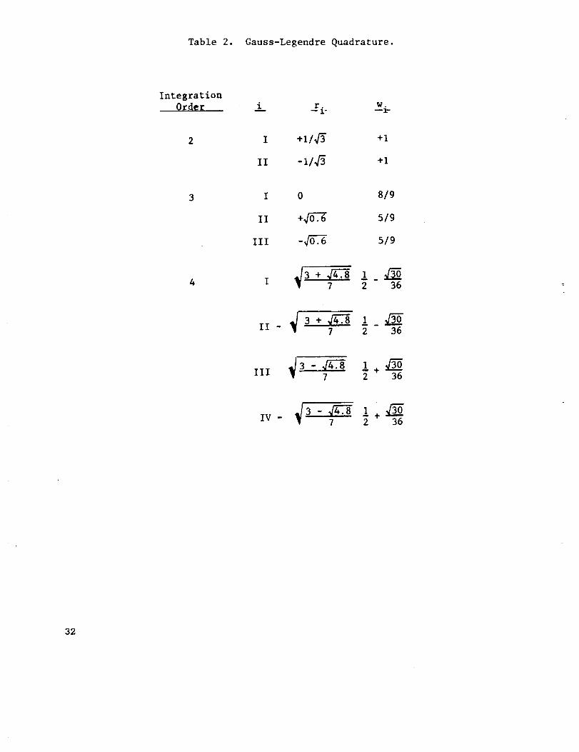
Table 2. Gauss-Legendre Quadrature.
Integration
Order mi _ x.r. _i-w-
I +I l_f3 +I
II -11_'3 +I
3 I 0 8/9
II +#-6"_6 5/9
III -#'6--.'6 5/9
V 31 + 4_.87 21 _-_36
i i - V 3 + 4_,.87 21 3_36
III
IV - V3 - 74_--._.8 21 + 3_36
32

Table 3, Newton-Cotes Quadrature.
b n
f F(r)dr = (b-a) E cn F. + Ri i n
o i=0
No. of
Intervals
nn n n n n n n
CO C I C2 C3 C4 C5 C6
1 Iu
2 2
2
3
i 4 !_ 6
! _3 _3 !8 8 8 8
4 7 32 12 32 __790 90 90 90 90
5 j_99 7__5 5__oo 5___o 7___5 ]__%9288 288 288 288 288 288
6 41 21__6 27 272 27 216 4__I840 840 840 840 840 840 840
33

For the stiffness matrix:
Kij ./+I j,+1 /+IBiDB j detJ drdsdt-1 -1 -1
where
Gij = BiDB j detJ
and D is the constitutive matrix
The body force is given by:
+I +i +1 T
FBI "/-1 I.l I_i Hi fB detJ drdsdt
where
Gi = HT fB detJ
and
[fB] T " [fBx FBy FBz]
The initial strain effect is given by:
Fo i =/+If+I/+1 BiDE o detJ drdsdt
-1 -I -I
where
r,i = BiD co detJ
and
[_o] T = [_x Cy Ez "_xy Yyz )ZX]
34

The "consistent" mass matrix is given by:
Mij=_I_:_I_:£:IoHTHjdetjdrdsdt
Where
Gij = pHTHjdetJ
The thermal strain effect is given by:
+I
FTHi : LI
+I +I
_1 _1 BTDETHdetJdrds°t
Where
TG i = BiD_THdetJ
And
T _y:T _ 0 0 0[ETH ] : [_x_T ^ z_T ]
The nonlinear strain effect is given by:
FNL i : i+I i+I i+I BT-I -I -1 iENL detJdrsdt
Where
T
Gi : BiDENLdetJ
And
[_NL] : [ _NLX _NLY CNLZ YNLXY YNLYZ YNLZX]
35
The surface traction effect is given by:
p+l e+l
H T . f dAFsri = j w sx s
-1 -I
Where the F . are the nodal forces due to surface tractions f on a surfacesrl s
of constant r. Similar expressions apply for surfaces of constant s or t.
dA =
m
8x
8s
8s
8._z8s
m
8._x8t
x, _ dsdt =' at
i
8t
m m
_z.8s 8t 8s 8t
8z 8x 8x 8z
8s 8t 8s 8t
8s 8t 8s 8t
dsdt
dA = Cdsdt
Then
Gi = H T. f CSl s
36
Large Deflection Theory
Second order engineering strain-displacement equations
e = _ + + { +X
Z ox I
e = _ + + 4
y _y 2 __y /
e
z :_+_ + -, +z_ \_/
_ _ _+ av av 8_ a_exy = 8y + 8x +l 8x 8y 8-_ 8y + 8xk--.
- z -- __ 8w 8w8_Zv 2#_ + 88u + + --eyz = 8z + 8y 8y
8w 8u 8u 8u 8v 8v 8w 8we =-- + -- .l ----+ ----+--
zx 8x 8z 8x 8z 8x 8z 8x&=m
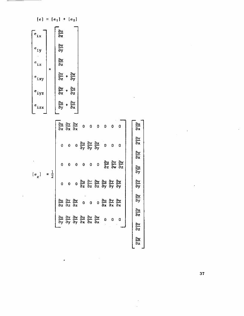
[e] = [ell + [e2]
eix I
e. I
zy
e.IZ
eixy ]
eiyzl
eizx I
n u
8u
8x
8y
8w
8z
8v 8w
8w 8u
8u _v
1[%] =
m
8u 8v 8w0 0 0 0 0 0
8x 8x 8x
8u 8v 8x0 0 0 0 0 0
8y 8y 8y
0 0 0 0 0 08u 8v 8w
8z 8w 8z
8u 8v 8w _u 8v 8W
o o o _-__-__ _y _y _y
8u 8v aw 8u 8v 8w0 0 0
8z 8z 8z 8x 8x 8x
8u 8v 8w 8u 8v 8w...... 0 0 08y 8y 8y 8x 8x 8x
m
8u
8v
8w
8__q8y
a_Xv
8y
8__w
8y
a_.p.u8z
I
._vj8z
8.._w8z
37

Let
38
d = au av awax 8x
d = 8u av 8waz az
[A]
X
= dl iY
dz_j
_T
IG II XI
OI
to-iT
_ _'r
101
d*l
"dl] TV!
[o]T
[._]T[o]T
[d_]T[o]T
[o]T
[d_]T[d_]T
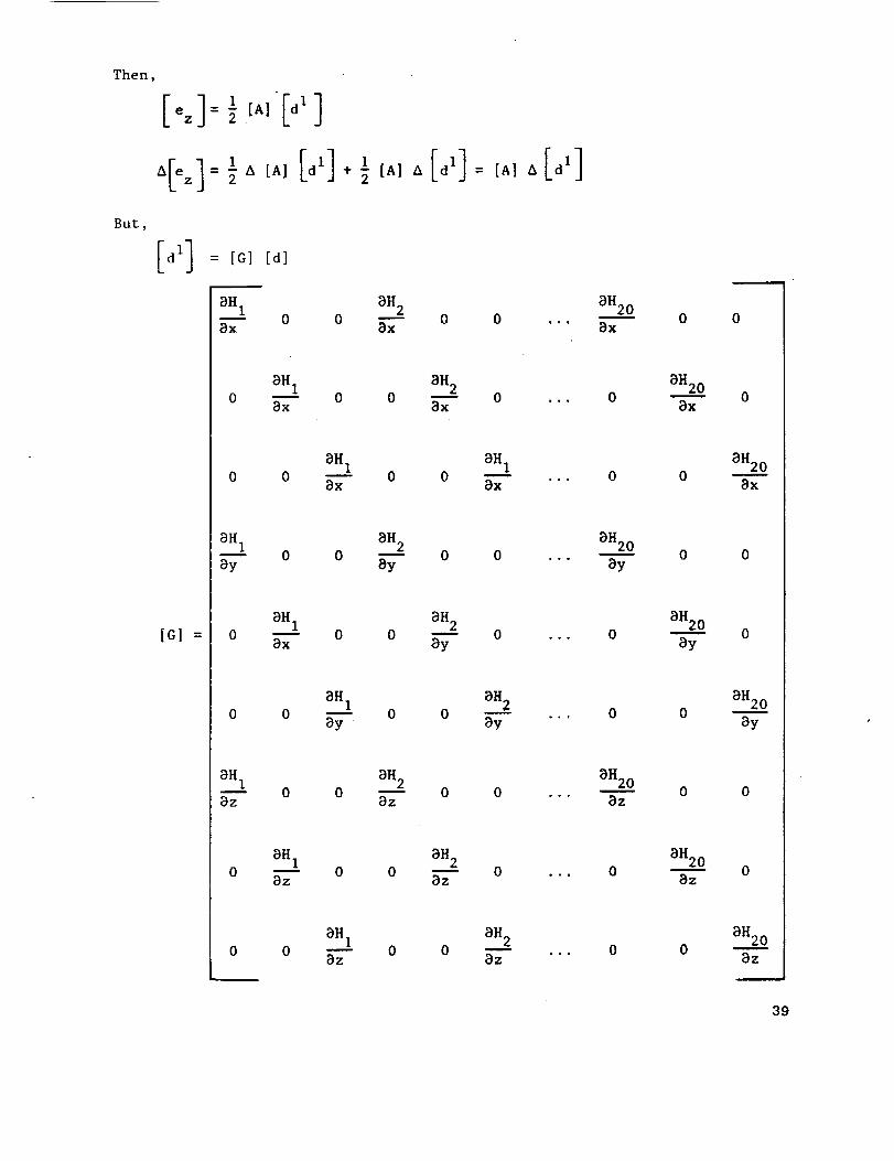
Then,
[,z]; ]
But
[G] =
8H 1 8H 20 0
ax 8x0 0
8H 1 8H 20 -- 0 0 -- 0
8x 8x
8H 1 8H 10 0 _ 0 0
8x 8x
8H 1 8H 20 0
8y 8y0 0
8H 1 8H 20 -- 0 0 -- 0
8x 8y
aH 1 _H_.__20 0 _ 0 0
8y 8y
8H 1 8H 20 0
8z 8z0 0
8H 1 8H 20 _ 0 0 _ 0
8z 8z
OH 1 OH20 0 _ 0 0 _ ,..
8z 8z
8H20
8x
8H20
8y
0
8H20
8z
0
0
0
8H20
8x
0
0
8H20
8y
0
0
8H20
8z
0
0
8H20
8x
0
0
8H20
8y
0
0
aH20
8z
39

So_
,, r_d']= tAl ,, _t_l tdJ_- tA1t_J'_Cdl
The incremental stiffness is
[R] :[_,].[q: [§l T [D] [B] dV
v
[q :/[q_ Io,[q_vv
The force unbalance is given by:
f(d) =[§l Is] dr- [_] = o
V
Where
[F] are the applied forces
a [el = IB] _ ld]
4O

But
And
A L,_:.f,'.,:_.I"'tsldv+ f_j_ ,,tsldvv
a [o] = [D] a[e] = [D] [§] a[d]
A [BI = A CB2]
Giving
A,,_: f_ [_]_,_v. ft_, + [m t_J_ [_,_vv v
Defining
[_s]_t_,: f[%]+,s,dvv
Gives
Then
For eigenvalue problems:
?_,]','=,oi+I,.,','
[_] ,,,:_,=f,o,'r,,,,,,,'r,s,_vv
41

But,
Then
[A] T IS] =
S 0 0x
0 S 0x
0 0 Sx
S 0 0xy
0 S 0xy
0 0 Sxy
S 0 0XZ
0 S- 0xz
0 0 Sxz
S 0 0 S 0xy xz
0 S 0 0 S 0xy xz
0
0 0 S 0 0 Sxy xz
S 0 0 S 0 0y yz
0 S 0 0 S 0y yz
0 0 S 0 0 Sy yz
S 0 0 S 0 0yz z
0 S 0 0 S 0yz z
0 0 S 0 0 Syz z
m
d 1x
A d 1Y
d 1z
[Ks]:/,oft ,M,Io,dvV
One of the major application areas for these graded material finite
elements will involve small linear elastic strains but extremely large dis-
placements. The severity of this condition is compounded by the involvement
of temperature effects and body forces, conditions which have not been
42

extensively addressed. Additionally, eigenvalue/eigenvector analysis is
required in the loaded conditions. We intend to take advantage of the sig-
nificant improvements in computer speed and memory size in attacking this
problem area.
We are using an incremental-updated Lagrangian approach. The virtual
work equation for the updated Lagrangian formulation leads to the nonlinear
incremental displacements from time (t) to time (t + &t).
At [C ijklSAEklA_ij - i °lJ 6 2AEtkAekj
_AUk _AUk ] /V- __ dV = _W(t + At) - t(Yij_AeljdV
where
6W(t + At) =ft(Fi + _i)_AUidV
(i)
(2)
+Lt(Ti + _i)_&Ui ds
A_ij -_ \_x'-'-T+ _xi/
Cijkl6AEklAeijdV is equivalent to
-2fv t oij6AeikAekjdV is equivalent to
(3)
{_u k} (4)
43

and
[KN1] { AUk } " (ft [BL] T [0"1] [BL] dV) l AUk}
At _lj6AUk'i'AUk'jdV is equivalent to
_J I__I(Lc__c__ _v)I_!
/Vt [BL]
where
t _ij6AgljdV is equivalent to
Ti_idv
(s)
(6)
(7)
(8)
IAolij" ["2] IA_"I0
TIAullj"[AUl,1AU1,2......%,3]
(9)
(i0)
_o._.[...._u__u;_u_...]_The incremental equilibrium is
where
[El] is the linear stiffness matrix, i.e.
(ii)
(12)
[KL] ._vt[BL] T [C] [BL] dV (13)
[KN] iS the nonlinear stiffness matrlx due to larger deformation, i.e.
44
[KN] : [KN1 ] + [KN2 ] (14)

[KNI] = /Vt [BL]T [(_I] [BL] dV
(15)
{API
" "_Vt [B2]T [O2] [B2] dV
is the incremental load from time (t) to (t + At) i.e.
- _(t+ At)-_ [BL]T 1o}dVt
(16)
(17)
The stress matrices are given by
[a] o
[02]
m
0
o [7] o
_ o o [o]_
(18)
[_]
- Oll
= 012
_ 013
o12 o13 -
(19)
[oi]
-2o22
(Symmetric)
0
-2033
-_2
-o12
0
- _ 1+°22 - i°13
- _ 2+03
m
-_13
0
- 01 3
1
i- -_.o12
- _- 33+Ol
(20)
45

Eigenvalue/Eigenvector Analysis
We are developing the algorithms for solving the lowest eigenvalue and
eigenvector pairs for large structure system of equations; that is,
K_ i = A i M@ i
where
K is the maximum symmetric stiffness matrix
M is the maximum symmetric mass matrix
A. is the ith eigenvaluei
_i is the ith eigenvector
The methodologies coded so far are the determinant search and subspace itera-
tion techniques.
Both of these techniques have been investigated extensively in a finite
element code that uses 8-noded shell elements and the COLSOL solution
scheme. The addition of the eigenvalue/eigenvector analysis capability is
closely linked to the solution procedure, and extensive changes to the COLSOL
routines were required. Both lumped mass and consistent mass matrices were
coded.
Determinant Search Method
In the determinant-search technique, a Sturm sequence check is very
useful for estimating the proper eigenshift. Once the proper eigenshift is
located in the neighborhood of the desired eigenvalue, a Rayleigh-quotient is
then employed to iterate the trial vector until convergence is reached. A
valid starting trial vector should be used, otherwise it may converge to the
wrong result even though the proper eigenvalue is obtained in the repeated
roots case. The logics for determining the proper eigenshift requires eigen
deflation, Gram-Schmidt orthogonality if necessary, and schemes of accelera-
tion, bisection, secant, or quadratic solutions. Appendix B shows the test
case results of this procedure.
Subspace Iteration
The subspace iteration technique employs vector transformation into
smaller q (n _ q _ m) eigen spaces, that is
46
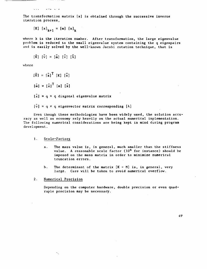
The transformation matrix [x] is obtained through the successive inverse
iteration process,
[K] [X]k+ 1 = [m] [x] k
where k is the iteration number. After transformation, the large eigenvalue
problem is reduced to the small eigenvalue system containing the q eigenpairs
and is easily solved by the well-known Jacobi rotation technique, that is
[;] = [&] [;]
where
[_1 = [_]T [K] [x]
[&] = [_]T [m] [_]
[x] = q x q diagonal eigenvalue matrix
Iv] = q x q eigenvector matrix corresponding [A]
Even though these methodologies have been widely used, the solution accu-
racy as well as economy rely heavily on the actual numerical implementation.
The following numerical considerations are being kept in mind during program
development.
I •
.
Scale-Factors
a. The mass value is, in general, much smaller than the stiffness
value. A reasonable scale factor (106 for instance) should be
imposed on the mass matrix in order to minimize numerical
truncation errors.
b. The determinant of the matrix [K - M] is, in general, very
large. Care will he taken to avoid numerical overflow.
Numerical Precision
Depending on the computer hardware, double precision or even quad-
ruple precision may be necessary.
47

3. Starting Trial Eigenvector
The starting trial eigenvector significantly affects the iteration
convergence rate. Most important is that the wrong trial eigenvec-
tot may lead to the wrong solution in the determinant search tech-
nique. In the subspace iteration technique, improper trial eigen-
vectors may skip some eigenpairs.
4. ConverRence Criteria Limits
a.
h.
c.
d.
Maximum number of iterations
Rayleigh-Quotient iteration tolerance
Eigenvector iteration tolerance
Solution convergence error tolerance
. The eigenshift for determinant search Rayleigh-quotient iteration
technique may converge to the wrong result if the proper eigenshift
is not determined. In order to determine the proper eigenshift for
the next eigenvalue, techniques should be investigated in order to
minimize the number of large matrix decompositions.
. Efficient decomposition and back substitution matrix decomposition
and back substitution play the most important role in the cost of
performing eigenvalue analysis.
48

Heat Transfer Development
Linear steady-state Equation:
at time step: t + At:
/e /s _s ht+Ate s dsD_ t+At
k e" dr +C
t+AtQe +/sc _s h t+Ateeds
X
r qs
where 8 "t =
K -"
"88 88 Be]8x 8y 8z
"Kx 1
0 0
0 Ky 0
0 0 K z
convection coefficient
surface of the body
49

governing equation: Linear heat transfer
e(KK + KC)Qt+At = Qt+At + Qt+At CA)
where KK - the conductivity matrix
m fV BmtKK = _=1 m • I_ Bm dVm (I)
K c - the convection matrix
m/.Kc= sch(m). Hs(m)T Hs(m). ds (m)
(II)
the nodal point heat flow input vector Q(t+At)
Qt+At = QB(t+At) + Qs(t+At) + Q (t+At)C
= _ fl H (m)T b(m) dVm
where QBt+At m jvm " 9t+At
(B)
(III)
fs S(m)Q (t+At) = m_ (m) HS(m)T qt+At " ds(m)
S 2
(IV)
where Qc(t+_t) - a vector of concentrated nodal point heat flow input
_J
50

e
The nodal point heat flow contribution Qt+At is due to the convection
boundary condition
b£ - the rate of heat generated in element
S
q - the surface heat flow input
At that time:
e(e) = H(e)t+At " 8t+At
es(e) = Hs(e)t+At 8t+&t
o(e) = B(e)t+At " et+_t
(la)
(Ib)
(lc)
where (e) _ denotes element m
®t+At---_ a vector of all nodal point temperatures at t+At
82t+A t 83t+& t em t+At ]
The matrix H(e)--_ Element Temperature
B(e)_ Temperature gradient interpolation matrice
Hs(e)---_ The surface temperature interpolation matrix
51

[B]--_derlvative of the shape function with respect to r, s, t and pre-
multiplication by J -1
e = I ; h ° Hs(m)T ° Hs(m) O (t÷_t) - dS (m)
Qt+At m jsc(m) " e
ee t+At The given nodal point environmental temperatures.
(v)
e
from this equation to find the Qt+At (i.e. 0e t+At and h are given)
Shape Function:
H1 = gl - (g9 + g12 + g17)/2
v
Y
3
4 I0_
5
2
18
6
H2 = g2 " (g9 + g10 + 818)/2
H3 = g3 " (gl0 + gll + g19)/2
H4 = g4 - (gll + g12 + g20)/2
H5 = g5 - (g13 + g16 + g17)/2
52

H6 = g6 - (g13 + 814 + g18)/2
H7 = g7 - (g14 + g15 + g19)/2
H8 = g8 - (g15 I+ g16 + g20)/2
H. = gi for ( i = 9 .... 20)1
gi = 0 if node i is not includes; otherwise:
gi = G(r, ri) G(s, si) GCt, ti)
G(_, _i ) = 1/2 (l+_i_) for _i = ± 1
G(_,_i) = (1-_ 2) for _i = 0
Jacobi's operator [J] is
The displacement functions:
X= 2H.x.
Y = X HiY i
Z=XH.z.1 ].
4
T
v
53

_t at at
w X
wher_:r_ s_ _ at_ the lbcar coordinates.
[B]:-_ _Hi
8r ar
aH.•a_ - 1
8s 8s
at at
H_- the rate of heat generated per unit volume
0 - the environmental temperaturee
sq: - the heat fiow input to the surface of the body
- the convecti6fl coefficient
"_ .¢q- =-h(O e - 0 s)
e - is the temperature of the body
_4

o(m) = H(m)t+At Ot+At
os(m) Hs(m)o= t+At
e-Cm) B (m)= " _t+_t
Ot+At - a vector of all nodal point
temperatures at t+_t
Tet+At = [elt+At e2 em] t+At
a)" from Equations (I), (II) we can find the
(Kk & K c)
(b): From Equation (B) the nodal point heat flow input
qt+At = QB(t+At) + qS(t+At) + qc(t+At)
where
/_qn b(m) dV(m)QB(t+At) = _ H(m)T _(t+At)
S Hs(m)T s(m) dS(m)Qs(t+At) = _ 2 " _(t+At)
Qc(t+At) - a vector of concentrated nodal point heat flow input
It can be solved for Q(t+&t)
(c): From Equation (V) the given nodal point environment temperatures
8e(t+At)
55

h _" Hs(m)T_ Hs(m) " _e (t+_t)e
dS (m)
ca_ solve for Q_t+At)(nodal pointheat distribution)
From _tems (a), (b), (c), substitute into Equation A.
(gk +!Kc) 9(t+At ) = Q(t+At) ÷ q_t+At)
The nodal point temperatures in each element can be found by using
equations (la), (Ib), (Ic).
ORIGINAL PAGE ISOF POOR QUALITY
56
E

I.I
l®
v
!-,
II II
J
It II II
%_d
% =
II _ Iml '_
0'
I
.,_
Iu
_ T_'1 .,4
Ztl
2"
÷
,I.
3.
V
®
9
÷
I
,o
÷
!
÷
*o÷
O"
II
4,
÷
v
5"/

A. Linear Steady-State:
• l,
Read Elem.
Connectivity
Material Prop.
Node Coordinates
Read Conductivity
Kx, Kyp Kz
Nodal Temperature 0.1
Heat Flux at Surface
sq
bHeat Generated Rate q
Convection Coefficient h
I iiiii _IDO I=i, NELM.
Transformation
of Conductivity
from Orthotropic
Axis to Local x, y, z
[K] = [A] T [km] [A]
Formed Conductivity
Matrix
[K] = BT - [K] • B
nxn
58
ORIG|_AL P._(}E IS
OF POOR QUALITY

i
Formed
[Kc] =/_ h - Hst • Ms • ds
[Kc] =EE w wnxn i j
(area) • h • H st • Hs
, ,,i
Formed
[Qe] h " Hst " (H s " 8e)dS
[qe] = rE w wnx 1 i j
(area) • H st - Ms • 8e
Formed
[QB ]=/v Ht " qb • dv
[QB ]
nx I
= ZZZ w • 5 • Wk • det [J] - H t • qb
Formed
[Qs ]= /s Hst "S
q • ds
[Qs]nx 1
=_ W. W. area • H st " qs1 3
59

T
..
Assemble the Matrix
into Structural Matrices
[ _k ] = E [K k]
[_c]=x [Kc]
E_ .1= EEQ]e e
[_]=xD ]B B
[_s] --_ [%] -ml
[iq o = [Q] I
Solve the Equation
o = [K] -1 [Q]
Use COLSOV Subroutine.m,..
l llf
Temp. Output
60
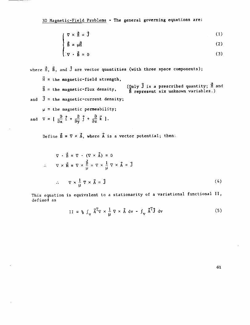
3D Magnetic-Field Problems - The general governing equations are:
V._=0
(1)
(2)
(3)
-> -->
where H, B, and _ are vector quantities (with three space components);
->
H = the magnetic-field strength,
->
B = the magnetic-flux density,
and J = the magnetic-current density;
(_nly _ is a prescribed quantity; H andB represent six unknown variables.)
and
p = the magnetic permeability;
v=[_x1+_a+ _ .
Define B = V x _, where _ is a vector potential; then:
°'o
_)V • B = V • (V x = 0
v× _ = v × __= v× iv× I = 3P P
! -> (4)•". V x V x A = JP
This equation is equivalent to a stationarity of a variational functional II,
defined as
II = ½ _v _TV x 1 V x _ dv - fv _T3 dvP
(s)
61

n
where _ = i_] Niai
N. = shape function of x, y, zl
N. = N. (x, y, z)i I
a. = the nodal value at Node i1
a. = a. (t)l i
where v is all space.
Define H = H + HS m
where
and
H = the magnetic source field,S
_ = the induced magentizations.m
The _ is any vector defined such thatS
V x _ = _ (6)s
then Equation 1 becomes:
->
V × H = 0 (7)m
This can be identically satisfied by introducing a scalar potential _ defined
by:
-9.
H = -V_m
.-9,
Eliminating B from Equations 2 and 3:
(g)
V • _ = V p_ = V IJ(_ s m )• • +H = 0
-V • pV_ + V • _s = 0 (9)
62
OR]GJNAL PAGE" IS
OF POOR QUALITY
T

For a simple scalar unknown
_= XN.a.I i
I _= _ (x, y, z, t)
where N. = N. (x, y, z)l l
a. = a. (t)1 i
Equation 9 may be written
V • pV¢ = _ (Px _(Py ay ) _(Pz
and, with the known quantity, written as:
f = V • p • Hs
For steady-state (time-dependent) problems, Equations I0 and 11 may be
rewritten:
(10)
(11)
_x)+ _ _ + _( (12)
S 1 + S 2 = F
Y
Boundary Conditions - Equation 12 is general and must be solved subject
to additional constraints on the boundary surface. On $1, if nonlinear
= _ (x, y, z, t),
63

¢ = ¢ (x, y, z) (13)
while the remaining part of the boundary has the following condition on S2
_x 88_xnx + _y _.n_yy + _z _z nz + g (x, y, Z) = 0 (14)
where n , n , and n are the direction cosines of the outward normal of the
x _ z SI and S 2 forms the complete boundary r, (Si + $2 = F).surface, and the union
Equation 13 is called Dirichlet condition, and Equation 14 is called Cauchy
boundary condition; if g = O, it is called Neumann boundary condition. A
field problem is said to have mixed boundary conditions when some portions of
F have Dirichlet while others have Cauchy.
In Equation 12, if _x =called Poisson's equation. Ify
equation.
= Pz =f = 0,
constant = p, ?z# = f(x, y, z)/_ is
then re# = 0 is known as the Laplace
Variational Principal - The function #(x, y, z) that satisfies Equations
12, 13, and 14 also minimizes the functional:
6I(@) = 0
+ 2f¢] dxdydz + fs2(g¢) dS2(15)
(16)
Element Equations - Suppose that the solution domain v is divided into
H elements of y nodes each. In each element, the unknown function may be
expressed by
Y (e)q(e)= i_l Ni@i = [N]{O} (17)
where #i is the nodal value of 0 at Node i. Equation 17 implies that onlynodal values of # are taken as nodal degrees of freedom, but derivatives of
may also be used as nodal parameters.
n (e)
I(¢) = Z I(¢ )
e=l
8I(_ (e))1 = O,
80 ii = I, 2, .... y
64

For a Node i on boundary $2, from Equation 15 we have on Surface $2 (e)"
#,B__(e)) B__(e) 8 8_ (e)) + ___(e) 8 (___(e)v_(e)[Px 85_x(e) __ + py (_y _z _i 8z
)a¢i "ax ay _i az
f B__(e) B__(e)
+ ] dr(e) + _(e) (g 8,i ) dS2a¢i(18)
If Node i does not lie on S2, the second integral does not appear.
to Equation 17, these terms typically become:
Y 8N i{ _x (e)= Z _ $i = [8N/Sxl{$}(e)
i=I
Referring
a rB___(e) aNi"8x ) = aW-
Thus on Surface S_ e) (Equation 14) we have:
aI(_ (e)) =
a¢ i
aN. aN i aN.
v_(e)[_x[aN/ax]{$}_-_ + _y[SN/ay]{$}B-_-- + pz[aN/Sz]{$}-_-? + fN i] dv (e)
+ _2(e ) ['Ni] dS2(e)
Let $ =_ Ni$i, then
65

8N i_= z EE- ¢i
8N.= Z i
ay _ _i
8N.
= Z _-i--$i
(19)
8y = [B(x,y, z)]¢i
where
[B(x, y, z)]=
8x 8x 8x
8N
8y 8y 8y
8N
8z 8z 8z
From Equation 19, this may be rewritten
where
Iv [s]T[kt][B]{¢} dv + Iv[fNi] dv + IS2[SN i] dS2 = 0
¢i
2
{¢}=
CY •
(nodal value)
(20)
66

Px 0 1
[k t ] = Py
0 Pz
[kt] = magnetic permeability on the principal axis (Px' Py' and pz ).
2.2.3 Task IIC - Graded Composite Materials
An investigation into the merits of various numerical integration schemes
has been pursued in order to determine which schemes might be best suited tothe calculation of stiffness matrices for elements composed of several layers
of different composite materials. All of the schemes investigated to this
point integrate by summing weighted properties evaluated at sampling points
which are spaced throughout the element volume. The differences between the
various schemes is in the weights associated with the sampling points and the
distribution of the sampling points.
The modularization of the stiffness routines allows fairly easy implemen-
tation of the various integration schemes. At present, the Gauss integration
schemes and Newton-Cotes integration schemes have been coded. In addition, a
selective Gauss integration scheme has been coded which uses different Gauss
integration orders for calculation of normal stress/strain terms than the
order used for shear stress/strain terms. Element stiffness matrices have
been obtained using these methods, and a consistent, accurate method for com-
paring them is being worked on.
The previously coded stiffness routines for the 8-, 16-, and 20-noded
isoparametric brick elements have been included in an existing finite-element
code, and an extended checkout has begun. Elastic test case runs of isotropic
materials have begun with comparisons to an existing finite-element code as
well as the critical results.
The test cases run to this point are from "A Proposed Standard Set of
Problems to Test Finite Element Accuracy," by R.H, HacNeal and R.L. Harder, a
paper presented at the 25th SDM Finite Element Validation Forum, May 14, 1984,
and are patch tests and cantilevered-element assemblages for eight-noded-brick
elements (Figures 11 - 13), Tables 4 and 5 summarize the results of some of
the test cases, and the theoretical results are presented in Table 6. It
should be noted that all of these cases were run using single precision.
Further improvement in the calculated answers is expected if double precision
is used, and this will be investigated in the future.
The 8-noded-brick results show that in the bending test cases the use of
incompatible modes produces a considerably better solution as measured by tip
displacement of the cantilevered beam model. However, the straightforward
inclusion of incompatible modes causes the element to fail the patch test, as
can be seen in the result for the existing code. An attempt to rectify this
problem was made in the CSTEM code and is reflected in the results. Here,
67

¥Outer DSmenstcms: klmtt Cube
[ • 1.0 st 106; v o .ZS
X
Locitlm of lamer taxies:
1 .Z49 .342 .192Z .826 .Z88 .Z883 .8SO .M9 .Z634 .Z?3 .?SO .nO5 .320 .IU .$436 .677 .305 .U37 .?M .H3 .6448 .165 .;45 .702
Iqoundar_ Cemdttton$: . • 10 .3 (Zx ,_ Jr ÷ Z)/2
v • 10.3 (x-_• z)/2
• - 10 .3 (x 4. Jr • 2z)/Z
Figure ii. Patch Test for Solids.
68
ORIGINAL P'._GE IS
OF POOR QUALITY

I I 1 ! 1 Ia) R_ular Shape _s
c) Parallelogram Shape (1merits
Length • (.0; Vtdth • 0._ Depth - 0.1
E - 1.0 x 10⁷; v - 0.3); Ilesh • 6 x 1
Loadtng: Untt forces at free end
Note: All elment.s have e4ual volume
Figure 12. Straight Cantilever Beam.
69

Inner Rjdtus.- 4.12; Outtr tHtus • 4.3_; Arc • gO"
Thickness • Go); [ • 100 ! |07; v • 0,)5; )ltSh • (S ! |
Loading: Unit forces it ttp
Figure 13. Curved Beam.
7O

Table 4, Existing FEMCode.
Eight-Noded Bricks
Patch Test
Without With
Incompatibles Compatibles
0% 15o%
% Error in Stress
Cantilevered Beam
Rectangular
Elements
Extension
In Plane
Out of Plane
Twist
Trapezc,idElements
Extension
In Plane
Out of Plane
Twist
Parallelogram
Elements
Extension
In Plane
Out of Plane
Twist
Without With
Incompatibles Compatibles
0.9856 (1.4%) 0.9875 (1.2%)
0.0928 (90.7%) 0.9922 (0.8%)
0.0252 (97.5%) 1.070 (7.0%)
0.8383 (16.2%) 0.7830 (21.7%)
0.9845 (1.5%) 1.007 (0.7%)
0.0040 (96.0%) 0.1855 (81.4%)
0.0067 (99.3%) 0.0286 (97.1%)
0.6075 (39.2%) 0.6507 (34.9_)
0.9846 (1.5%) 1.011 (1.1%)
0.0543 (94.6%) 0.7284 (27.2%)
0.0084 (99.2%) 0.6367 (36.3%)
0.4541 (54.6%) 0.7584 (24.2%)
Curved Beam
In Plane
Out of Plane
0.0732 (92.7%) 0.9498 (5.0%)
0.2249 (77.5%) 0.7874 (21.3%)
Normalized Tip Displacement (% Error)
71

Table 5. CSTEM Stiffness Code.
Eight-Noded Bricks
Patch test
Without With
Incompatibles Compatibles
0% 0%
% Error in Stress
Cantilevered_Beam
Rectangular
Elements
Extension
In Plane
Out of Plane
Twist
Trapezoid
Elements
Extension
In Plane
Out of Plane
Twist
Parallelogram
Elements
Extension
In Plane
Out of Plane
Twist
Without With
Incompatibles Compatibles
0.9856 (1.4%) 0.9875 (1.2%)0.0928 (90.7%) 0.9922 (1.8%)0.0252 (97.5%) 0.9081 (9.2%)0.8394 (16.1%) 0.8186 (18.1%)
0.9845 (1.5%) 1.007 (0.7%)
0.0040 (96.0%) 0.1851 (81.5%)
0.0067 (99.3%) 0.0285 (97.1%)
0.6078 (39.2%) 0.6502 (35.0%)
0.9846 (1.5%) 1.009 (0.9%)
0.0543 (94.6%) 0.7343 (26.6%)
0.0084 (99.2%) 0.5960 (40.4%)
0.4543 (54.6%) 0.8008 (19.9%)
Curved Beam
In Plane
Out of Plane
0.0733 (92.6%) 0.9520 (4.8%)
0.2265 (77.4%) 0.8771 (12.3%)
Normalized Tip Displacement (% Error)
72

Table 6. Theoretical Solutions.
Patch Test
_x = ey + _z = yxy = _0/z = yzx = 10 -3
ox = oy = gz = 2000 psi, Ixy = lyz = Izx = 400 psi
Straight Beam
Extension
In Plane
Out of Plane
Twist
(Tip Displacement in Direction of Load)
3.0 x I0-5 in.
0. 1081 in.
0. 4321 in.
0.00341 in.
Curved Beam (Tip Displacement in Direction of Load)
In Plane 0.08734 in.
Out of Plane 0.5022 in.
73

the incompatible modesare included in the stiffness matrix and thus in the
solution of the system of equations. This improves displacements; however,
the recovery of stress from the displacement solution doesn't include
incompatible modes, so the patch test is satisfactory. Along with other
possibilities, this technique is still being investigated.
Another observation that can be made is the reinforcement of the fact
that modeling technique can greatly influence the results. This is evident
from the use of trapezoid- and parallelogram-shaped elements to solve the
same cantilever beam problem. A trapezoid-shaped element in particularshould be avoided in view of the bad results.
The 20-noded brick passes the patch test with no problem regardless of
integration order or whether single or double precision is used. The 20-noded
brick is a quadratic displacement element by nature, and so there are no
incompatible modes associated with it. The problem with the patch test as
exhibited in the 8-noded brick is then avoided by the 20-noded brick.
The regular beam was used for the remainder of the investigation.
Because of the single layer of elements, reduced integration produces poor
results when looking at displacements. This is due to the presence of zero
energy modes: spurious nodal displacements which still satisfy the elemental
equations at the Gauss points. More than one layer of elements would help to
eliminate this phenomena due to the continuity of the element boundaries.
It was found that the use of single or double precision would greatly
affect the results as can be seen in the tabulated results, Table 7. This
points to a numerical sensitivity to rounding off or truncation. Using the
CSTEM code, attempts were made to improve the results by performing certain
operations in double precision while the majority of operations remained in
single precision. It was finally found that the best improvement was obtained
by calculating the shape functions using double precision while all other
operations remained single precision.
2.2.4 Task liD - I/0 and Solution Techniques
To achieve computational efficiency and to avoid repeated codings, a
modular equation solver has been written to perform combinations of the fol-
lowing functions:
Matrix decomposition (matrix triangularization)
Force vector reduction and back-substitution
Matrix decomposition and force vector back-substitution
Partial matrix static condensation
Matrix determinant and Sturm sequence count.
Investigations of the eigenvalue/eigenvector large deformation structural
problem were conducted. Two popular techniques were studied: determinant
search and subspace iteration.
7d

oZI
,'-4
Z1'--4
"ii0
w
o
o
_J
gg_o
6 g _ _! !
o _ _ _
_J
_ 0
0
tD
I,.i0
"0
o_
o
o
wu_ aJ
_Jw
m o
1.a
"11
6_6o
o_ o_ o_ o0
6 6 _ o
_oo
o0 o 000 _D 0'_ ,,d"o_ oO 0 I_.
o _ _ _a,,._ _ _ ,_
_ o
0
75

Determinant Search - This technique employs inverse iteration in conjunc-
tion with eigenshift and Rayleigh quotient method. This method relies heavily
on the equations solver to compute Sturm sequence checks and matrix determi-nants. The starting trial eigenvector plays a very important role in converg-
ing to the appropriate corresponding eigenpair. Orthogonality criteria must
be imposed for computing repeated, or cluster, eigenpairs.
Subspace Iteration - This method employs inverse iteration, subspace
transformation, and Jacoby successive rotation. Besides the efficient equa-
tions solver, this method relies heavily on the stiff/mass ratio and conver-
gence criteria. This method will generally compute the desired eigenpairs,
but it may not guarantee the lowest eigenpairs.
Constraint equations play a very important role in solving boundary value
problems. Two techniques have been developed for solving FEM structural prob-lems with constraints. The first technique is the so-called "penalty func-
tion" method which treats the constraint equation as a stiff finite element
and is very easy to incorporate in the program, such as:
To construct a fairly stiff symmetric stiffness matrix out of the
given linear constraint equation
To assemble the constraint stiffness matrix into the global overall
structural stiffness matrix.
The technique generally yields satisfactory solutions as long as the
number of constraints is not large.
The second technique is the classical matrix partitioning method. For
computational efficiency, Gauss elimination is used to perform static con-
densation rather than using matrix inversion to effect matrix partitioning
and reduction. This method is mathematically exact and should be employed
when the number of constraints becomes large. However, implementation of
this technique into the program may be complicated due to the variation of
structural modelings.
For those stress computations within the finite element, Lagrange inter-
polation demonstrated very good results when data are interpolated or extrapo-
lated from the known Gaussian quadrature quantities.
In order to extend the program capability from static analysis to eigen-
value/eigenvector dynamic analysis, the assembly of consistent mass matrices
is required. Because of the similarity between element stiffness matrix and
element consistent mass matrix_ the assembly routines were extended to accom-
modate either.
A new data :file structure has also been added to the CSTEM stiffness
routines. The investigation into different integration techniques emphasized
the need to base storage of certain data on the integration point, rather than
the element as previously done. This is due to the fact that the number of
integration points may vary from element to element, depending on the inte-
gration scheme used. The new data-file structure was incorporated into the
76

code used for the preceding investigations, so installation can be considered
complete.
2.2.5 Task liE - Stand-Alone Codes
These capabilities are being generated as stand-alone codes while the
development continues. The major effort in this area is the development of
the file structure and data flow for this complex, interconnected problem. A
change in the file structure is under consideration as a result of the larger
number of integration points being considered. The present element-based
file structure will not adequately handle this problem.
77


APPENDIX A - ACCUMULATED LITERATURE
AEBG Literature Search
I ° Allen, D.H., "Predicted Axial Temperature Gradient in a Viscoplastic
Uniaxial Bar Due to Thermomechanical Coupling," Texas A&M University,
HM 4875-84-15, November 1984.
2. Allen, D.H. and Haisler, W.E., "Predicted Temperature Field in a Thermo-
mechanically Heated Viscoplastic Space Truss Structure," Texas A&M
University, MM 4875-85-I, January 1985.
3. Kersch, U., "Approximate Reanalysis for Optimization Along a Line," Int.
J. Num. Meth. Engrg., Vol. 18 pp 635-650, 1982.
. Berger, M.A. and McCullough, R.L., "Characterization and Analysis of the
Electrical Properties of a Metal-filled Polymer," Composites Science and
Technology, 22, pp 81-106, 1985.
° McCullough, R.L., "Generalized Combining Rules for Predicting Transport
Properties of Composite Materials," Composites Science and Technology,
22, pp 3-21, 1985.
. Minagawa, S., Nemat-Nasser, S., and Yanada, M., "Dispersion of Waves in
Two-Dimensional Layered Fiber-Reinforced, and other Eleastic Composites,"
Computers and Structures, Vol. 19, No. 1-2, pp 119-128, 1984.
. Oliver, J. and Onate, E., "A Total LaGrangian Formulation for the Geo-
metrically Nonlinear Analysis of Structures using Finite Elements. Part
I Two-Dimensional Problems: Shell and Plate Structures," Int. J. Num.
Meth. Eng., Vol. 20, pp 2253-2281, 1984.
. Adams, D.F. and Crane, D.A., "Combined Loading Micro-Mechanical Analysis
of a Unidirectional Composite," Composites, Vol. 15, No. 3, pp 181-192,
1984.
, Ni, R.G. and Adams, R.D., "A Rational Method for Obtaining the Dynamic
Mechanical Properties of Laminae for Predicting the Stiffness and Damping
of Laminated Plates and Beams," Composites, Vol. 15, No. 3, pp 193-199,
1984.
10. Reddy, J.N. and Chandrosheklara, K., "Nonlinear Analysis of Laminated
Shells Including Transverse Shear Strains," AIAA J., Vol. 23, No. 3, pp
440-441, 1985.
11. Pedersen, P. and Jorgensen, L., "Minimum Mass Design of Elastic Frames
Subjected to Multiple Load Cases, "Computers and Structures Vol. 18,
No. i, pp 147-157, 1984.
79
_._]NT_NTIONALLY _L _,'t
PRECEDING PPlGE BLANK NOT FILMED

12.
13.
14.
15.
16.
17.
18.
19.
20.
21.
22.
23.
24.
25.
80
Maymon, G., "Response of Geometrically Nonlinear Elastic Structures to
Acoustic Excitation - An Engineering Oriented Computational Procedure,"
Computers and Structures Vol. 18, No. 4, pp 647-652, 1984.
Nomura, S. and Chow, T.W., "Bounds for Elastic Moduli of Multiphase
Short-Fiber Composites," ASME Journal of Applied Mechanics, Vol. 59,
pp 540-545, 1984.
Bert, C.W. and Gordaninejad, F., "Forced Vibration of Timoshenco Beams
made of Multimodular Materials," ASME Journal of Vibration, Acoustics,
Stress, and Reliability in Design, Vol. 107, pp 98-105, 1985.
Takenti, Y., Furukawa, T., and Tanigawa, Y., "The Effect of Thermoelastic
Coupling for Transient Thermal Stresses in a Composite Cylinder," ASME
Journal of Vibration, Acoustics, Stress, and Reliability in Design, Vol.
106, pp 529-532, 1984.
Abondi, J° and Benveniste, U., "Constitutive Relations for Fiber-
Reinforced Inelastic Laminated Plates," ASME Journal of Applied
Mechanics, Vol. 51, pp 107-113, 1984.
Wilson, E.L., Taylor, R.L., Doherty, W.P., and Ghabonski, J., Incompat-
ible Displacement Models," Numerical and Computer Methods in Structural
Mechanics, Academic Press, 1973.
MacNeal, R.H. and Harder, R.L., "A Proposed Standard Set of" Problems to
Test Finite Element Accuracy," 25th SDM, Finite Element Validation Forum,
May 14, 1984.
Casey, J.K., Moore, C.L., and Bartlett, J.C., "Automatic Improvement of
Design (AID) User's Manual," General Electric R67FPD214, May 1967.
Platt, C.E., Pratt, T.K., and Brown, K.W., "Structural Tailoring of
Engine Blades (STAEBL)," NASA CR-167949, June 1982.
Zienkiewicz, O.C. and Nayak, G.C., "A General Approach to Problems of
Large Deformation and Plasticity using Iso-Parametric Elements," 3rd
Conference on Matrix Methods in Structural Mechanics, Wright Patterson
Air Force Base, October 19-21, 1971.
Mondkar, D.P. and Powell, G.H., "3D Solid Element (Type 4 - Elastic or
Elastic-Perfectly-Plastic) for the ANSR-II Program," NSF/RASO0293, July
1980.
Chamis, C.C. and Minich, M.D., "Structural Response of Fiber Composite
Fan Blades," ASME 75-GT-78, 1975.
Bathe, K.J., Finite Element Procedures in Engineering Analysis_ Prentice-
Hall, Inc., Englewood cliffs, New Jersey, 1982.
Khot, N.S., "Optimality Criterion Methods in Structural Optimization,"
AFWAL-TR-81-3124, October 1982.

26
27.
28.
29.
30.
31.
32.
33.
34.
35.
Jense, P.S. and Loden, W.A., "Supplementary Studies on the Sensitivity ofOptimized Structures," AFWAL-TR-81-3013,March 1981.
Batt, J.R., Gellin, S., and Gellatly, R.A., "Force Method Optimization
II, Volume I - Theoretical Development," AFWAL-TR-82-3088 Volume I,
November 1982.
Batt, J.R., Dale, B.J., Skalski, S.C., Witkop, D.L., and Gellin, S.,
"Force Method Optimization II, Volume II, User's Manual,"
AFWAL-TR-82-3088, Volume II, November 1982.
Bushnell, D., "Computerized Analysis of Shells - Governing Equations,"
AFWAL-TR-81-3048, December 1981.
Chari, M.V.K., Berkery, K.F., and Ogle, M.D., "Finite Element Evaluation
of Power Losses in Electrical Devices of Axisymmetric Cross-Section,"
General Electric R81CRDI68, July 1981.
Flanagan, G.V., "Composite Laminate Weight Optimization on the HX-20,"
AFWAL-TR-83-4061, August 1983.
Flanagan, G.V. and Park, W.J., "Composite Laminate Weight Optimization
on the Sharp PC-1500 Pocket Computer," AFWAL-TR-83-4095, August 1983.
McKnight, R.L., "Poroloy Shroud Analysis," General Electric R73AEG323,
1973.
Chang, F.K., Scott, R.A., and Springer, G.S., "Strength of Bolted Joints
in Laminate Composites," AFWAL-TR-84-4029, March 1984.
Boyd, Harris, King, and Welch, Electronic Countermeasures_ Peninsula
Publishing, 1978.
Emerson and Cuming 1982 Products Catalog.
Krueger, C.H., "A Computer Program for Determining the Reflection and
Transmission Properties of Multilayered Plane Impedance Boundaries,"
AFWAL-TR-67-191, September 1967.
Contributed by Texas A&M Consultants
I ,
.
Duhamel, J.M.C., "Memoire sur le calcul des actions moleculaires
developpees par les changements de temperature dans les corps solides,"
Memories par divers savans_ vol. 5, pp 440-498, 1838.
Neuman, F., Vorlesungen uver die Tjeorie der Elasticitat der festen
Korper und des Lichtathers t pp 107-120, Leipzig, 1885.
81

. Boley, B.A., "Survey of Recent Developments in the Fields of Heat Con-
duction in Solids and Thermo-Elasticity," Nuclear Ekngineering and
Design, Vol. 18, pp 377-399, 1972.
. Danilovskaya, V.I., "Thermal Stresses in an Elastic Half-Space Arising
After a Sudden Heating of its Boundary," Prikl. Mat. Mekh., Vol. 14, pp316-318, 1950.
"On " Prikl5. Danilovskaya, V.I., a Dynamic Problem of Thermoelasiticity, .
Mat. Mekh., Vol. 16, pp 341-344, 1952.
6. Boley, B.A. and Weiner, J.H., Theory of Thermal Stresses, Wiley, New
York, 1960.
7. Coleman, B.D., "Thermodynamics of Materials with Memory," Archives for
Rational Mechanics and Analysis, Vol. 17, pp 1-46, 1964.
• " Journal of8 Takeuti, Y., "Foundations for Coupled Ther_oelasticity,
Thermal Stresses, Vol. 2, pp 323-339, 1979.
9. Boley, B.A., "Thermal Stresses Today," source unknown.
I0. Bargmann, H., "Recent Developments in the Field of Thermally Induced
Waves and Vibrations," Nuclear Engineering and Design, Vol. 27,
pp 372-385, 1974.
II. Chester, M., "Second Sound in Solids," Physics Review, Vol. 131,
pp 2013-2015, 1963.
12. Biot, M.A., "Thermo-elasticity and Irreversible Thermodynamics," Journal
of Applied Physics, Vol. 27, pp 240-251, 1956.
13. Blot, M.A., "New Methods in Heat Flux Analysis with Application to Flight
Structures," Journal of Aeronautical Sciences, Vol. 24, pp 857-874, 1957.
14. Zienkiewicz, O.C. and Cheung, Y.K., "Finite Elements in the Solution of
Field Problems," The Engineer, Vol. 220, pp 507-527, 1965.
15. Wilson, E.L. and Nickell, R.E., "Application of the Finite Element Method
to Heat Conduction Analysis," Nuclear Engineering and Design, Vol. 4,
pp 276-286, 1966.
16. Fraeijs de Veubeke, B.M. and Hogge, M.A., "Dual Analysis for Heat
Conduction Problems by Finite Elements," International Kournal for
Numerical Methods in Engineering, Vol. 5, pp 65-82, 1972.
17. Aguirre-Ramirez, G. and Oden, JOT., "Finite Element Technique Applied
to Heat Conduction in Solids with Temperature Dependent Thermal Conduc-
tivity," International Journal for Numerical Methods in Engineering,
Vol. 7, pp 345-355, 1973.
82
=

18.
19.
20.
21
22
23
24
25
26
27
28
29.
30.
Wilson, E.L., Bathe, K.J., and Peterson, F.E., "Finite Element Analysis
of Linear and Nonlinear Heat Transfer," Nuclear Engineering and Design
Vol. 29, pp 110-124, 1974.
Bruch, J.C. Jr. and Zyvoloski, G., "Transient Two-Dimensional Heat Con-
duction Problems Solved by the Finite Element Method," International
Journal for Numerical Methods in Engineering, Vol. 8, pp 481-494, 1974.
Comini, G., Del Guidice, S., Lewis, R.W., and Zienkiewicz, O.C., "Finite
Element Solution of Non-linear Neat Conduction Problems with Special
Reference to Phase Change," International Journal for Numerical Methods
in Engineering, Vol. 8, pp 613-624, 1974.
Donea, J., "On the Accuracy of Finite Element Solutions to the Transient
Heat-Conduction Equation," International Journal for NuMerical Methods
in Emgineering, Vol. 8, pp 103-110, 1974.
Kohler, W. and Pittr, J., "Calculation of Transient Temperature Fields
with Finite Elements in Space and Time Dimensions," International Journal
for Numerical Methods in Engineering, Vol. 8, pp 625-631, 1974.
Wood, W.L. and Lewis, R.W., "A Comparison of Time Marching Schemes for
the Transient Heat Conduction Equation," International Journal for
Numerical Methods in Engineering, Vol. 9, pp 679-689, 19,5.
Hughes, T.J.R., "Stability of One-Step Methods in Transient Nonlinear
Heat Conduction," Transactions of the 4th International Journal for
Numerical Methods in Engineering, Vol. 9, pp 679-689, 1975.
Bathe, K.J. and Khoshgoftaar, R., "Finite Element Formulation and
Solution of Nonlinear Heat Transfer," Nuclear Engineering and Design,
Vol. 51, pp 389-401, 1979.
Hogge, M.A., "Secant Versus Tangent Methods in Nonlinear Heat Transfer
Analysis," International Journal for Numerical Methods in Engineering,
Vol. 16, pp 51-64, 1980.
Chung, K.S., "The Fourth-Dimension Concept in the Finite Element Analysis
of Transient Heat Transfer Problems," International Journal for Numerical
Methods in Engineering, Vol. 17, pp 325-325, 1981.
Parkus, H., "Methods of Solution of Thermoelastic Boundary Value Problems
in High Temperature Structures and Materials," Proceedings of the Third
Symposium on Naval Structural Mechanics, 1964.
Lord, H.W. and Shulman, Y., "A Generalized Dunamical Theory of Thermo-
elasticity," Journal of Mechanics and Physics of Solids, Vol. 15,
pp 299-309, 1967.
Achenbach, J.D., "The Influence of Heat Conduction on Propagating Stress
Jumps," Journal of Mechanics and Physics of Solids, Vol. 16, pp 273-282,
1968.
83

31.
32.
33.
34.
35.
36.
37.
38.
39.
40.
41.
42.
Oden, J.T., "Finite Element Analysis of Nonlinear Problems in the
Dynamical Theory of Coupled Thermoelasticity," Nuclear Engineering
and Design, Vol. 10, pp 465-475, 1969.
Oden, J.T. and Kross, D.A., "Analysis of General Coupled Thermoelasticity
Problems by the Finite Element Method," Proceedings 2nd Conference on
Matrix Methods in Structural Mechanics, AFFDL-TR-68-150, pp I091-I120,1969.
Oden, J.T., Chung, T.J., and Key, J.E., "Analysis of Nonlinear Thermo-
elastic and Thermoplastic Behavior of Solids of Revolution by the Finite
" Proceedings 1st International Conference on StructuralElement Method,
Mechanics and Reactor Technology, Berlin, 1971.
Allen, D.J. and Milly, T.M., "A Comparison of Constitutive Models for
Nonlinear Rate Dependent Material Behavior of Solids," Virginia Poly-
technic Institute and State University, Report No. VPI-E-81-16, 1981.
Burnett, J.A. and Padovan, J., "Residual Stress Fields in Heat-Treated
Case-Hardened Cylinders," Journal of Thermal Stresses, Vol. 2, pp
251-263, 1979.
Cernocky, E.P. and Krempl, E., "A Coupled, Isotropic Theory of Thermo-
viscoplasticity Based on Total Strain and Overstress and its Predictions
in Monotonic Torsional Loadings, "Journal of Thermal Stresses, Volo 4,
pp 69-82, 1981.
Inoue, T., Nagaki, S., and Kawate, T., "Successive Deformation of a Vis-
coelastic-Plastic Tube Subjected to Internal Pressure under Temperature
Cycling," Journal of Thermal Stresses, Vol. 3, pp 185-198, 1980.
Huang, S. and Cozzarelli, F.A., "Some Analytical and Numerical Results
for Cladded Fuel Rods Subjected to Thermoirradiation Induced Creep,"
State University of New York at Buffalo, Noo 105, 1979.
. . "A Theory of Thermoviscoplasticity BasedCernocky, E.P. and Krempl, E ,
on Infinitesimal Total Strain," International Journal of Solids and
Structures, Vol. 16, pp 723-741, 1980.
Mukherjee, S., Kumar, V., and Kuang, J.C., "Elevated Temperature Inelas-
tic Analysis of Metallic Media Under Time Varying Loads Using State Vari-
able Theories," International Journal of Solids and Structures, Vol. 14,
pp 663-679, 1978.
Perzyna, P., "Fundamental Problems in Viscoplasticity," Advan. Appl.
Mech. Vol. 9, pp 243-377, 1966.
Zienkiewicz, O.C and Courmeau, I.C., Visco-P!asticity--Plasticity and
Vreep in Elastic Solids--A Unified Numerical Approach," International
Journal for Numerical Methods in Engineering, Vol. 8, pp 821-845, 1974.
84
%

43.
44.
45.
46.
47.
48.
49.
50.
51.
52.
53.
54.
55.
Lee, D. and F. Zaverl, Jr., "A Generalized Strain Rate Dependent Consti-
tutive Equation for Anistropic Metals," Acta. Met., Vol. 26, No. II,
p 1171, 1978.
Pugh, C.E., Corum, J.M., Lin, K.C., and Greenstreet, W.L., "Currently
Recommended Constitutive Equations for Inelastic Design Analysis of FFTF
Components," ORNL TM-3602, Oak Ridge National Laboratory, September 1972.
Valanis, K.D., "A Theory of Viscoplasticity Without a Yield Surface, Part
I - General Theory," Archives of Mechanics, Vol. 23, pp 517-533, 1971.
Laflen, J.H. and D.C. Stouffer, "An Analysis of High Temperature Metal
Creep: Part I - Experimental Definition of an Alloy and Part II - A
Constitutive Formulation and Verification," ASME J. Eng. Mat. & Tech.
I00, p 363, 1978.
Walker, K.P., "Representation of Hastelloy-X Behavior at Elevated Temper-
ature with a Functional Theory of Viscoplasticity," presented at ASME
Pressure Vessels Conference, San Francisco, Aug. 12, 1980 (Also to appear
in ASME Journal of Engineering Materials and Technology).
Hart, E.W., "Constitutive Relations for the Nonelastic Deformation of
Metals," ASME J. Eng. Mat. & Tech. 98-H, p 193, 1976.
Krieg, R.D., Swearengen, J.C., and Rohde, R.W., "A Phsically-Based Inter-
nal Variable Model for Rate-Dependent Plasticity," Proceedings ASME/CSME
PVP Conference, pp 15-27, 1978.
Bodner, S.R. and Partom, Y., "Constitutive Equations for Elastic-Visco-
plastic train-Hardening Materials," Journal of Applied Mechanics, Vol.
42, No. 2, pp 385-389, 1975.
Miller, A.K., "An Inelastic Constitutive Model for Monotonic, Cyclic, and
Creep Deformation: Part I - Equations Development and Analytical Pro-
cedures and Part II - Application to Type 304 Stainless Steel," ASME J.
Eng. Mat. & Tech. 98-H, p 97, 1976.
Lou, Y.C. and Schapery, R.A., "Viscoelastic Characterization of a Non-
linear Fiber-Reinforced Plastic," Journal of Composite Materials, Vol. 5,
pp 208-234, 1971.
Schapery, R.A., "A Theory of Non-Linear Thermovisco-elasticity Based on
Irreversible Thermodynamics," Proceedings 5th U.S. National Congress on
Applied Mechanics, pp 511-530, 1966.
Schapery, R.A., "On a Thermodynamic Constitutive Theory and Its Appli-
cation to Various Nonlinear Materials," Proceedings IUTAM Symposium, pp
259-285, 1968.
Bouc, R. and Geymonat, G., "Linearized Thermoviscoelasticity with High
Temperature Variations and Related Periodic Problems," International
Journal of Engineering Science, Vol. 16, pp 681-705, 1978.
85

56.
57.
58.
59.
60.
61.
62.
63.
64.
65.
66.
67.
68.
Frutiger, R.L. and Woo, T.C., "A Thermoviscoelastic Analysis for Circular
Plates of Thermorheologically Simple Material," Journal of Thermal
Stresses, Vol. 2, pp 45-60, 1979.
Herrman, K. and Hattheck, C., "Thermal Stresses in the Unit Cell of a
Fiber-Reinforced Material," Journal of Thermal Stresses, Vol. 2, pp
179-191, 1963.
Gurtin, M.E., "Variational Principles in the Linear Theory of Visco-
elasticity," Archive for Rational Mechanics and Analysis, Vol'. 3, pp
179-191, 1963.
Leitman, H.J., "Variational Principles in the Linear Theory of Visco-
elasticity," Archive for Rational Mechanics and Analysis, Vol. 3, pp
179-191, 1963.
Reddy, J.N., "Modified Gurtin's Variational Principles in the Linear
Dynamic Theory of Viscoelasticity," International Journal of Solids and
Structures, Vol. 12, pp 227-235, 1976.
Zienkiewicz, O.C. and Godbole, P.N., "Flow of Plastic and Visco-Plastic
Solids with Special Reference to Extension and Forming Processes," Inter-
national Journal for Numerical Methods in Engineering, Vol. 8, pp 3-16,1974.
Williams, J.R., Lewis, R.W., and Morgan, K., "An Elasto-Viscoplastic
Thermal Stress Model with Applications to the Continuous Casting of
Metals," International Journal for Numerical Methods in Engineering,
Vol. 14, pp 1-9, 1979.
Sprinatha, H.R. and Lewis, R.W., "A Finite Element Method for Thermo-
viscoelastic Analysis of Plane Problems," Computer Methods in Applied
Mechanics and Engineering, Vol. 25, pp 21-33, 1981.
Allen, D.H. and Haisler, W.E., "A Theory for Analysis of thermoplastic
Materials," Computers & Structures, Vol. 13, pp 124-135, 1981.
Yamada, Y., "Constitutive Modelling of Inelastic Behavior and Numerical
Solution of Nonlinear Problems by the Finite Element Method," Computers
& Structures, Vol. 8, pp 533-543, 1978.
Snyder, M.D. and Bathe, K.J., "Formulation and Numerical Solution
of Thermo-Elastic-Plastic and Creep Problems," National Technical
Information Service, No. 82448-3, 1977.
Newman, J.B., Giovengo, J.F., and Comden, L.P., "The CYGRO-4 Fuel Rod
Analysis Computer Program," Transactions of the 4th International Con-
ference on Structural Mechanics in Reactor Technologu, D I/I, 1977.
Kulak, R.F., Belytschko, T.B., Kennedy, T.H., and Schoeberle, D.F.,
"Finite Element Formulations for the Thermal Stress Analysis of Two-
86

69.
70.
71.
72.
73.
74.
75.
76.
77.
78.
79.
80.
and Three-Dimensional Thin Reactor Structures," Transactions of the 4thInternational Conference on Structural Mechanics in Reactor Technology,E 3/3, 1977.
Kulak, R.F. and Kennedy, J.M., "Structural Responseof Fast Reactor CoreSubassemblies to Thermal Loading," 3rd International Conference onStructural Mechanics in Reactor Technology, E I/6, 1975.
Spaas, H.A.C.M., Mjuazono, S., Kodaira, T., and Ito, K., "Theoretical and
Experimental Analysis of Sodium Cooled Nuclear Reactor Nozzle Loaded by
Thermal Shocks," 3rd International Conference on Structural Mechanics in
Reactor Technology, G I/5, 1975.
GHlkan, P. and Akay, H.U., "Analysis of Prestressed Concrete Reactor
Vessels under High Thermal Gradient," 3rd International Conference on
Structural Mechanics in Reactor Technology, H 2/4, 1975.
Cost, T.L. and Heard, J.M., "Finite-Element Analysis of Coupled Thermo-
viscoelastic Structures Undergoing Sustained Periodic Vibrations," AIAA
Journal, Vol. 16, pp 795-799, 1978.
Truesdell, C. and Toupin, R., "The Classical Field Theories,"
Encyclopedia of Physics, Vol. III/I, 1960.
Truesdell, C. and Noll, W., "The Nonlinear Field Theories of Mechanics,"
Encyclopedia of Physics, Vol. 111/3, 1965.
Coleman, B.D. and Roll, W., "The Thermodynamics of Elastic Materials with
Heat Conduction and Viscosity," Archive for Rational Mechanics Analysis,
Vol. 13, pp 167-178, 1963.
Kuznetsov, V.N., Ogibalov, P.M., and Pobedrya, B.E., "The Coupling Prob-
lem in Polymer Mechanics," Mikhanika Polimerov, Vol. I, pp 59-65, 1971.
Bykov, D.L., ll'yusbin, A.A., Ogibalov, P.M., and Pobedrya, B.E., "Some
Fundamental Problems of the Theory of Thermoviscoelasticity," Mikhanika
Polimerov, Vol. I, pp 41-58, 1971.
Kovalenko, A.D. and Karnaukhov, V.G., "A Linearized Theory of Thermo-
viscoelasticity," Mekhanika Polimerov, Vol. 2, pp 214-221, 1972.
Navarro, C.B., "Asympototic Stability in Linear Thermoviseoelasticity,"
Journal of Mathematical Analysis and Applications, Vol. 65, pp 399-431,
1978.
Chang, W.P. and Cozzarelli, F.A., "On the Thermodynamics of Nonlinear
Single Integral Representations for Thermoviscoelastic Materials with
Applications to One-Dimensional Wave Propagation," Acta Mechanica, Vol.
25, pp 187-206, 1977.
87

81.
82.
83.
84.
85.
86.
87.
88.
89.
90.
91.
92.
93.
Lee, C., Chang, W.P., and Cozzarelli, F.A., "Some Results on the One-
Dimensional Coupled Nonlinear Thermoviscoelastic Wave Propagation Problem
with Second Sound," Acta Mechanica, Vol. 37, pp 111-129, 1980.
Turkan, D. and Mengi, Y., "The Propagation of Discontinuities in Non-
Homogeneous Thermoviscoelastic Media," Journal of Sound and Vibration,
Vol. 70, pp 167-180, 1980.
Nunziato, J.W. and Walsh, E.K., "Amplitude Behavior of Shock Waves
in a Thermoviscoelastic Solid," International Journal of Solids and
Structures, Vol. 15, pp 513-517, 1979.
Young, R.W., "Sensitivity of Thermomechanical Response to Thermal Bound-
ary Conditions and Material Constants," International Journal of Solids
and Structures, Vol. 15, pp 513-517, 1979.
Ting, E.C. and Tuan, J.L., "Effect of Cyclic Internal Pressure on the
Temperature Distribution in a Viscoelastic Cylinder," International
Journal of Mechanical Sciences, Vol. 15, pp 861-871, 1973.
Young, R.W., "Thermomechanical Response of aViscoelastic Rod Driven by a
Sinusoidal Displacement," International Journal of Solids and Structures,
Vol. 13, pp 925-936, 1977.
Mukherjee, S., "Variational Principles in Dynamic Thermoviscoelasticity,"
International Journal of Solids and Structures, Vol. 9, pp 1301-1316,
1973.
Reddy, J.N., "Variational Principles in Dynamic Thermoviscoelasticity,"
International Journal of Solids and Structures, Vol. 9, pp 1301-1316,
1973.
Reddy, J.N., "A Note on Mixed Variational Principles for Initial-Value
Problems," Quarterly Journal of Mechanics and Applied Mathematics, Vol.
28, 1975.
Oden, J.T. and Reddy, J.N., Variational Methods in Theoretical Mechanics,
Springer-Verlag, New York, 1976.
Batra, R.C., "Cold Sheet Rolling, The Thermoviscoelastic Problem, A
Numerical Solution," International Journal for Numerical Methods in
Engineering, Vol. II, pp 671-682, 1977.
Batra, R.D., Levinson, M., and Betz, E., "Rubber Covered Rolls - The
Thermoviscoelastic Problem. A Finite Element Solution," International
Journal for Numerical Methods in Engineering, Vol. I0, pp 767-785, 1976.
Oden, J.T., "Finite Element Approximations in Nonlinear Thermovisco-
elasticity," NATO Advanced Study Institute on Finite Element Methods in
Continuum Mechanics, Lisbon, 1971.
88

94.
95.
96°
97.
98
Oden, J.T., Finite Elements of Nonlinear Continua, McGraw-Hill, New
York, 1972.
Oden, J.T., Bhandari, D.R., Yagawa, G., and Chung, T.J., "A New Approachto the Finite-Element Formulation and Solution of a Class of Problems in
Coupled Thermoelastoviscoplasticity of Crystalline Solids," Nuclear
Engineering and Design, Vol. 24, pp 420-430, 1973.
Strung, G. and Matthies, H., "Numerical Computations in Nonlinear
Mechanics," presented at the Pressure Vessels and Piping Conference,
ASME, No. 79-PVP-I03, San Francisco, 1979.
Allen, D.H., "Predicted Axial Temperature Gradient in a Viscoplastic
Uniaxial Bar Due to Thermomechanical Coupling," Texas A&M University, MM
4875-84-15, November 1984.
Allen, D.H., and Haisler, W.E., "Predicted Temperature Field in a
Thermomechanically Heated Viscoplastic Space Truss Structure," Texas A&M
University, MM 4875-85-I, January 1985.
89

qik
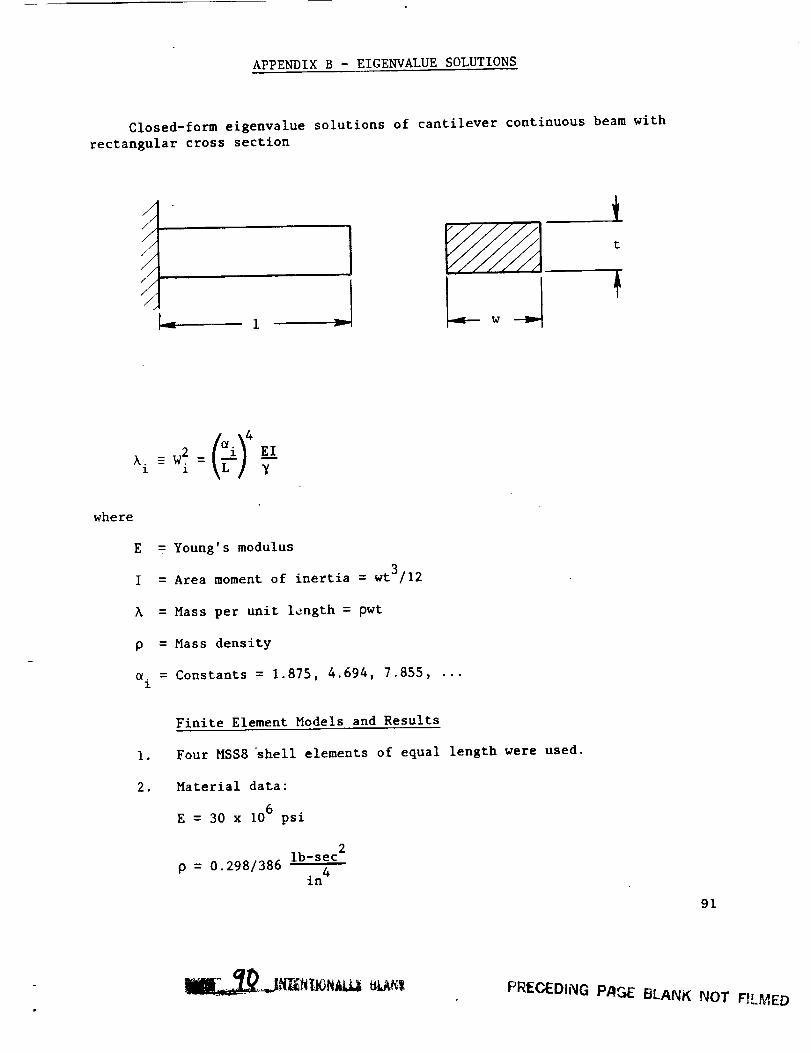
APPENDIX B - EIGENVALUE SOLUTIONS
Closed-form eigenvalue solutions of cantilever continuous beam with
rectangular cross section
///
/
i
where
E
I
= Young's modulus
= Area moment of inertia = wt3/12
= Mass per unit length = pwt
p = Mass density
_. = Constants = 1.875, 4.694, 7.855, ...i
2.
Finite Element Models and Results
Four MSS8 shell elements of equal length were used.
Material data:
E = 30 x 106 psi
ib-sec 2
0 = 0.298/386 4in
91
PRECEDING P.'_C._E BLAtYK _JOT F,..t_rD_ '-

3. Constant cantilever dimensions:
4_
L=8 in.
W=2 in.
Results :
Test Case Thickness
t = 2 in.
Theoretical
k I = 39
k2 = 1535
MSS8
A 1 = 38.9
k 2 = 1014
t= 1 in.A 1 = 9.77
A2 = 384
A 1
X2
= 10.3
= 347
t=0.2 in.
A 1 = 0.39
A 2 = 15.4
A3 = 120
A I
A2
k3
= 0.42
= 15.7
= I18
92

APPENDIX C - EIGENSHIFT AND RAYLEIGH QUOTIENT EXAMPLE
/
/////
L=8 in.
------_ X
tt=2 in.
Y
E = 30 x l0 s psi, v = 0.3, p = 0.298 x l0 s lb/in 3
i
Mode
Shape
(Axis-About)
Ist Bend E
Ist Bendy
Ist Tors X
2nd Bend Z
2nd Bendy
Ist Axial X
3rd Bend E
3rd Bendy
Eigen Values
Eigenvalue Shift and
Subspace Iterations Rayleigh Quotient
0.357145302
0.362975676
6.24068457
9.53697761
0.3+0
0.4- 0
6.0+0
8.0+0
I0.0 - 0
16.0 - 0
44+0
49+049.4069934
.057320891
.037155197
.24067101
.79694164
.46902631
.98479339
.82830848
.40698682
93

Form Approved
REPORT DOCUMENTATION PAGE OMBNo.070.01a8Public repo_ burdenfor this co#t_ec_onof InformationIs estimated to average 1 hourper response, includingthe time for mvlew_g insb'uctions,searchingexistingdata sources,gatheringand malnlainlr_ the data needed, and completinglind reviewing the collectionof information. Send commentsregardingthis burden estimate or any other aspect of thiscollectionof i_focmatton,includingsuggestionsfor reducingthis burden, to WashingtonHeadquarters Services,Directoratefor informationOperationsand Reports, 1215 JeffersonDavis Highway,Suite 1204, Arlk_gton,VA 22202-4302, and to the Office of Management and Budget,Paperwork ReductionProject (0704-0188), Washington,DC 20503.
1. A(_ENCY USE ONLY i/_ea_'_a_) ..... 2. REI;OR'T DATE 3. REPORT TYPE AND DATES COVEi_ED
April 1992 Final Contractor ReportL
4. TITLE AND SUBTITLE 5. FUNDING NUMBERS
Coupled Structural/Thermal/Electromagnetic Analysis/Tailoring of
Graded Composite Structures
First Annual Status Report WU-505-62-91
6. AU'rHo_fi(Si' C-NAS3--24538
R.L. McKnight, P.C. Chen, L.T. Dame, H. Huang, and M. Hartle
7. PERFOI_MING ORGANIZATION NAME(S) AND ADDRESS(ES)
General Electric
Aircraft Engine Business GroupCincinnati, Ohio 45215
9. SPONSORING/MONITORING AGENCY NAMES(S) AND ADDRESS(ES)
National Aeronautics and Space AdministrationLewis Research Center
Cleveland, Ohio 44135-3191
11. SUPPLEMENTARY NOTES
8. PERFORMING ORGANIZATION
REPORT NUMBER
None
!10. sPoNsoRING/MONITORINGAGENCY REPORTNUMBER
NASA CR-189150
Project Manager, C.C. Chamis, Structures Division, NASA Lewis Research Center, (216) 433-3252.
'1'2a. DiSTRIBUTIONIAVAILkBILITY STATEMENT
Unclassified - Unlimited
Subject Category 39
12b. DISTRIBUTION CODE
13. ABSTRACT (Maximum 200 words)
Accomplishments are described for the first year effort of a 5-year program to develop a methodology for coupled
structural/thermal/electromagnetic analysis/tailoring of graded composite structures. These accomplishments
include: (1) the results of the selective literature survey; (2) 8-, 16-, and 20-noded isoparametric plate and shell
elements; (3) large deformation structural analysis; (4) Eigenanalysis; (5) anisotropic heat transfer analysis; and
(6) anisotropic electromagnetic analysis.
14. SUBJECT TERMS
Literature survey; Solid elements; Plate elements; Large deformation; Eigenanalysis;
Anisotropic; Heat transfer; Electromagnetic analysis; Graded composites
17. SECURITY CLASSIFICATION 18. SECURITY CLASSIFICATION 19. SECURITY CLASSIFICATION
OF REPORT OF THIS PAGE OF ABSTRACT
Unclassified Unclassified Unclassified
NSN 7540-01-280-5500U.S. C,-OVERNMENTPRINTING OFFICE: 1992 - 750-034/60307
15. NUMBER OF PAGES
10216. PRICE CODE
A0620. LIMITATION OF ABSTRACT
Standard Form 298 (Rev. 2-89)
Prescribed by ANSI Std. Z39-18298-102


![[X] EXPEDITE](https://img.dokumen.tips/doc/110x75/6290ebe975ad8d306424d00c/x-expedite.jpg)