Embed Size (px)
Citation preview

NASA Contractor Report 194457CU--CSSC-93-06-II
Coupled Structural, Thermal, Phase-Change andElectromagnetic Analysis for SuperconductorsVolume II
C.A. Felippa, C. Farhat, K.C. Park, C. Militello, and J.J. SchulerUniversity of ColoradoBoulder, Colorado
January 1996
Prepared forLewis Research CenterUnder Grant NAG3-934
National Aeronautics and
Space Administration
https://ntrs.nasa.gov/search.jsp?R=19960015528 2018-09-06T04:41:13+00:00Z


TABLE OF CONTENTS
VOLUME II
Part I - Parametrized Variational Principles for Linear Electromagnetodynamics.
Abstract .................................................. 1
Introduction ................................................ 2
Field Equations ............................................. 4
Six-Field Variational Principles .................................. 7
Seven-Field Functionals ....................................... 13
Finite Element Discretization ................................... 19
Conclusions ................................................ 25
References ................................................. 27
Part II - Finite Element Analysis of Time-Independent Superconductivity,
Ph.D. thesis, Report CU-CSSC-93-02, Center for Space Structures
and Control, College of Engineering, University of Colorado,
Boulder, Colorado, 1993.
Abstract ................................................. 29
Introduction ................................................ 31
EM and Four-Potential Theory .................................. 45
Current Density Predicting Four-Potential Theory .................... 61Thermal Effects ............................................. 81
The Clemld Finite Element .................................... 101
The Clem2d Finite Element .................................... 114
The Cupleld Finite Element ................................... 134
The Superconducting Finite Element ............................. 155
The Thermal Problem ........................................ 192
Coupled Thermal-EM Problem in Normal Conductor ................. 218
The Complete Coupled Problem ............................... 231
Conclusions ................................................ 264
References ................................................. 271

S_Y
Describedare the theoretical development and computer implementation of reliable and efficient
methods for the analysis of coupled mechanical problems that involve the interaction of mechanical,
thermal, phase-change and electromagnetic subproblems. The focus application has been the
modeling of superconductivity and associated quantum-state phase-change phenomena. In support
of this objective the work has addressed the following issues: (1) development of variational
principles for finite elements, (2) finite element modeling of the electromagnetic problem, (3) coupling
of thermal and mechanical effects, and (4) computer implementation and solution of the
superconductivity transition problem. The main accomplishments have been: (1) the development
of the theory of parametrized and gauged variational principles, (2) the application of those principled
to the construction of electromagnetic, thermal and mechanical finite elements, and (3) the coupling
of electromagnetic finite elements with thermal and superconducting effects, and (4) the first detailed
finite element simulations of bulk superconductors, in particular the Meissner effect and the nature
of the normal conducting boundary layer. The theoretical development is described in two volumes.
Volume I describes mostly formulations for specific problems. Volume II describes generalization
of those formulations.
i±

PART I
PARAMETRIZED VARIATIONAL PRINCIPLES
FOR LINEAR ELECTROMAGNETODYNAMICS
ABSTRACT
Two families of paramet_rizvd mixed variational principles for linear electmmagnetodynamics am
constructed. The first family is applicable when the current density distribution is known a priori. Its
six independent fields are magnetic intensity and flux density, magnetic potential, electric intensity
and flux density and electric potential. Through appropriat_ specialization of parameters the first
principle reduces to more conventional principles proposed in the literature. The second family is
appropriate when the current density distribution is an additional unknown, giving a total of seven
independently varied fields. In this case it is shown that a conventional variational principle exists
only in the time-independent (static) case. Two static functionals with reduced number of varied
fields are investigated. The application of one of these principles to construct finite elements with
current prediction capabilities is illustrated with a numerical example.

1. INTRODUCTION
The application of energy and variational methods in electroma_etodynamics to construct
finite element approximations has not received to date the same level of attention gained in con-
tinuum and structural mechanics. Part of this lag can be attributed to the dominance of analytical
and semi-analytical methods. Over the past century (since Heaviside's landmark papers) these
methods have been refined and tuned to routinely treat special but important classes of application
problems such as circuits, antennas and waveguides. The most comprehensive exposition of EM
energ3, methods in book form is that of Hammond [1 ], who applies these methods to hand-computed
Rayleigh-Ritz and Galerkin approximations.
The use of EM finite elements has received modest but increasing attention for calculations that
involve multidimensional, complex geometries and intricate field distributions. Much of the work
to date appears to have been done in England, most likely because of the strong influence of the
Swansea *_r_up formerly headed by O. C. Zienkiewicz. The work is well described in survey articles
by Davies [2], Trowbridge [3], Simkin and Trowbridge [4] and the textbook by Silvester and Ferrari
[5]. The overall impression given by these expositions is that of an unsettled subject, reminiscent
of the early period (1955-1968) of finite elements in structural mechanics. ! A great number
of single-field formulations based on flux, intensity, scalar and reduced potentials are described
with the recommended choice varying according to the application, medium involved (polarizable,
dielectric, semiconductors, etc.) number of space dimensions, temporal variation characteristics
(static, quasi-static, harmonic or transient) as well as other factors of lesser importance.
The present work is part of an ongoing research project to develop one- and two-dimensional
finite element models for superconductors [6--8]. During the course of this project several variational
principles of increasing generality were constructed. This paper presents a partial unification of
mixed variational principles for linear electromagnetics. Two families of parametrized variational
principles are considered. These two families, identified by the number of independently varied
fields in the sequel, are intended for two different _ of source data.
The six-field family is appropriate when the current density distribution J is a source field (that
is, is known a priori). Its general functional is denoted by .-
Rc6)(E,D, B, H, A, ¢), (I)
where E, D, B and H are theclassicalelectromagneticfieldsthatappear inMaxwelrs equations,
and • and A aretheelectroma_maeticpotentials.Thisfunctionalisfound todepend on 21 numerical
coefficientsthatspecifythe weights of variousfields.The coefficientsmust satisfy12 consistency
constraints,leaving9 freeparameters.Through appropriatespecializationof theseparametersall
specificfunctionalsof thisform thatcontainthepotentialsA and _ as independentfieldscan be
produced. These functionalsare applicabletobothstaticand dynamic problems.
i For example; mixed multifietd variational principles are not mentioned.
2

The seven-field family is a generalization of R (6) that is appropriate when the current density
distribution J is unknown. Its general functional is denoted by
R (7) (E, D, B, H, A, *, J). (2)
This functional depends on 36 coefficients that must satisfy 24 constraints, apparently leaving
12 free parameters. These constraints, however, can only be fully satisfied only if the system is
time-independent; thus a variational principle of the assumed quadratic form exists only in the
static case. For the dynamic case a four-field restricted variational principle in the sense of Rosen-
Prigogine can be readily constructed. For static problems specialized principles with two to four
variables are investigated. One of these static principles is applied to the finite element calculation
of current distribution in a wire of varying conductivity.
The two families do not exhaust 2 the totality of variational principles for linear electromagnetics
because two classes of functionals are excluded:
(I) Functionals in which the distribution of volume charges is also varied independently are not
covered. The techniques of Sections 3 and 4 can be applied to derive an eight-field family
that provides a true variational principle for the static case. This principle would have limited
practical application, however, because in electrostatics free charges migrate to the surface of
conductors; consequently the internal charge distribution is known to be zero. It is doubtful
whether conventional principles for the dynamic case exist.
(17) Functionals that lack the EM potentials A and q_ as independently varied fields are not covered.
These would be analogous to the complementary energy principles of mechanics. Although
occasionally used for bound estimation purposes, complementary EM principles lack ap-
peal in our research program because of three reasons: (1) A and • appear naturally in the
volume-source and boundary-closure terms, (2) potentials are excellent variables to treat ma-
terial interface discontinuities in finite element discretizations, and (3) A is a key variable in
superconductor modeling.
Extensions of the present variational principles to nonlinear and coupled-field problems are
outlined in the Conclusions. Our main research thrust has been the generalization to the highly
nonlinear problem of superconductivity. Such problems usually display a mix of conducting and
superconducting regions. As a result the current density varies enormously in space. Finding this
distribution, which reflects the separation of the material into normal and superconducting regions,
is an essential part of the problem. It follows that the seven-field family is of particular interest as a
point of departure for constructing variational principles for superconductors. Such developments
will be reported in a sequel paper.
2 Thus the qualification "partial unification" used above.

2. FIELD EQUATIONS
The Maxwell Equations
The Maxwell equations of electromagnetodynarnics, developed in the I860s, are used here
in the classical '3+1' format. These equations involve six space-time fields: B, D, E, H, J and
p. Vectors E and H represent the electric and magnetic field strengths (also called intensities),
respectively, whereas D and B represent the electric and magnetic flux densities, respectively) All
of these are three-vector quantities, that is, vector fields in three-dimensional space (xt ----x, x2 --
y X3 -_ Z):
_1 DI El} {HIB= B2 , D= D2 , E= E2 , H= /'/2 (3)
B3 D3 E3 /'/3
Each component may depend on space and time. Other field quantities are the total current density
J (a three-vector) and the electric free-charge density p (a scalar). Using superposed dots to denote
differentiation with respect to time t, we can state Maxwell's equations in afixed Galilean frame 4
VxH-D=J,
V.B=0,
VxE+B=0,
V.D=p,(4)
in which the use of a rnks-Giorgi system of units is assumed: The first three equations are also
called Ampere-Maxwell, Faraday's and Gauss' laws, respectively.
The system (4) supplies a total of eight partial differential equations, which as stated are
independent of the properties of the underlying medium. If J and p are prescribed source fields the
eight equations are insufficient, however, to determine the twelve spatial components of fields B,
D, E and H.
Constitutive Equations
The field intensities E and H and the corresponding flux densities D and B are not independent
but connected by electromagnetic constitutive equations. For an etectromagnetically isotropic
material the equations are
I B=/_H, D=EE. ] (5)
B is also called the mag-netic induction vector and D the electric displacement vector. Many authors
note, however, that the last term may be highly misleading.
Corrections, whether relativistic or not, required as a result of the motion of the reference system arenot considered here.
5 In a cgs-unit system, factors of 4rr appear in the nonhomogeneous Maxwell equations.

where/_ and_ arethepermeabilityandsusceptibility,respectively,of thematerial6. Thesecoeffi-cientsmaybefunctionsof positionbut(for staticor harmonicfields)donotdependon time. For ageneralnon-isotropicmaterialboth_ andEbecometensors.Evenin isotropicmediatx may be a
complicated function of H; in ferromagnetic materials that exhibit hysteretic effects/x depends on
the previous magnetization history.
In free space # =/x0 and _ = E0, which are connected by
c_ = 1/(/x0Eo), (6)
where co is the speed of light in vacuum.
Many conductors, obey Ohm's law, which relates the electrical field strength E to the current
density J:
[ J:_E, J (7)
where a is the conductivity of the material. Again for a non-isotropic material a is generally a tensor
that for time-harmonic fields may contain real and imaginary components; in which case the above
relation becomes a generalized Ohm's law. In the sequel cr is assumed to be time-independent. For
good conductors cr > > _; for bad conductors o" < < E. In free space, cr -- O.
The Electromagnetic Potentials
The electric scalar potential • and the magnetic vector potential A are introduced by the
standard definitions
E=-Vq_-A, B=VxA, ] (8)
upon which the two homogeneous Maxwell equations in (4) become identically satisfied. The
definition of A leaves its divergence V • A arbitrary. A common choice to fix A is the Lorentz
gauge:
V. A _ 0. (9)+ _zE
With this choice the two non-homogeneous Maxwell equations written in terms of * and A
separate into the wave equations
V2<_ -- _,E_ ) --" --p/E, VZA - tzE.4, = -/_J, (10)
For a conducting medium, these equations are indirectly coupled on the right-hand side through
Ohm's law (7).
6 Other names for these quantities, such as inductivity and permittivity, are also used
5

Summary of Field Equations
For furtheruse in the derivation of variational principles, we summarize and label the field
equations as follows:
MH: V×H-D-J=0,
Mo: V.D-p=0,
C_ : D-eE= 0,
C. : B-/zH = 0,
PE: E+v_+A =0,
Ps: B-VxA=0,
Co: E-crJ= O,
MB: V.B=0,
ME: V×E+B=0,
GL : V-A+/zE_ = 0.
(11)
The set (MH, Mo, C,, C_, Pe, [8) supplies 16 equations for the 5 x 3 + 1 = 16 unknown
spatial components of (E, D, B, H, A, q_). Equations (Ms, ME) are in fact redundant, being iden-
tically satisfied by (PE, Ps). Equation GL is only a normalization condition on A. Ohm's law Ca
may be adjoined if the current density J is not given, in which case we obtain 19 equations for 19
unknown component functions.
Notational Conventions
In the following derivation of parametrized variational principles, the notational conventions
of references [9-13] are followed. An independently varied field is identified by a superposed
tilde; for example E, B. A derived field is identified by writing its independent "parent" field as
superscript; for example:
D e = eE, B A -- V x A, H A --/z-lB A =/z-Iv x A. (12)
If a derived quantity depends on two parent fields, both are listed starting with the most
significant one:
D ¢'A -- EE ¢'A = -E(V_ +/ix). (13)
The integral of a function f over volume V or surface S is often abbreviated to
6

Integralsoverspace-timeV x [tl, t2] or S x [tt, t2] may be shortened to
If f, g are two vector functions, their inner-product over V may be abbreviated in the usual
manner:
( f'gv=) d '/vfTgdV' (16)
and similarly for surface, volume x time, and surface x time integrals.
3. SIX-FIELD VARIATIONAL PRINCIPLES
The functionals considered in this and following sections have the general form
I R=U-P+B=L+BI (XT)where U is a quadratic form that characterizes the internal (stored) energy of the electromagnetic
field, P is a linear form that characterizes the potential of volume-source contributions, and B
contains boundary closure integrals. We often use L (the volume Lagrangian) for U - P.
The first two components can be expressed as space-time integrals:
£L () £LU= Lt d V dt = IA P= 79 d V dt (79)Vxtv×t' = , (18)
where/,4 and 79 are the electromagnetic energy density and source density, respectively. We also
denote 12 =/,4 - 79 as Lagrangian volume density. The boundary closure term is treated later as it
emerges from the first variation of L = U - P. The functionals and densities in (17) and (18) will
be superscripted with the number of independent fields as appropriate.
The six-field source density is given by
79(6) = jr A + p¢_, (19)
because J and p are prescribed. As for L4<6), making use of the "undetermined coefficient template"
technique of references [ 11-13], the following parametrized form is postulated: 7
c-lH s
c-tH A
5D e
D _a
T -gllI
g21I
g31I
g41I
gslI
_ g611
g12I gt3I gl41 gIsI g16I-
g22I g23I g24I gzsI g26I
g32I g33I g34I g35I g36I
g42I g43I g44I g45I g46I
g52I g53I g54I g55I g56I
g62I g63I g64I g65I g66I_
• cB H
cB
cB a
' E O
E
E *a
(20)
Following a nomenclature similar to that used in developing parametrized variational principles for
continuum mechanics, L4 may be called the generalized electromagnetic field energy density. As a
rough _maide in comparing to such principles, c-tH and D may be regarded as analogous to mechanical
stresses whereas cB and E are analogous to mechanical strains. The potentials A and _ are analogous
to displacements. The analogy, however, does not readily extend to boundary conditions.

where gij are dimensionless scalar coefficients to be selected, I denotes the 3 x 3 identity matrix
and
c2= 1/(/xE), (21)
is the speed of propagation of EM disturbances in matter. The scaling of B and tt by c and c- l in
(19) "equilibrates" the physical units. The derived fields that appear there are:
B _ =/xH, B A=Vx_,, E D=6-15, E _A=-V_-A,,
H a =/x-lB, H A -----/_-IBA -----/Z-IV X A, D e = EE, D *_ = _E *A.(22)
Relations (22) may be expressed in matrix form as
cB n
cB
cB A
E o
I
E_, A
-/xcI 0 0 0 0 0 "]
0 cI 0 0 0 0 ]
0 0 cA 0 0 0 ._.
0 0 0 E-ll 0 0
0 0 0 0 I 0 E0 0 -0_I 0 0 -V
or
(23)
¢- fi [c-tH s
¢-IHA
D e
D*a
-c-lI 0 0 0 0
o (/xc)-LI 0 0 0
0 0 (/xc)-tA 0 0
0 0 0 I 0
0 0 0 0 E1
0 0 - O.._:EI 0 0OI
o §oo 5o E
-EV
(24)
in which A ----V x denotes the curl operator for typographical convenience; note that A T _ - x V.
Let
'H
§
Z(6) = A_
D
E
¢,
, C (6) =
CII C12 C13 C14 C15 C16-
C21 C22 C23 C24 C25 C26
C31 C32 C33 C34 C35 C36
C41 C42.. C43 C44 C45 C46
C51 C52 C53 C54 C55 C56
C61 C62 C63 C64 C65 C66 _
(25)
be the complete 16-component state vector of six independent fields and the 16 x 16 kernel matrix,
respectively, obtained by changing the variables in (20) according to (23) and the transpose of (24).
Then
_//(6) _. 1Z(6) TC(6)Z(6)" (26)
8

The component submatrices of C (6) are given by
Ctt = gtt/zI, El2 = g12I,
C14 = g_4txcI, C15 = gtsc -lI,
C21 = g21I, C22 = g22/x-lI,
C24 = g24ci, Cz5 = g25ecI,
0
Cl3 = g13A - gl6c-t _-)"I,
C16 -" -g16 c-IV,
a
C23 -" g23/_-IA- - g26Ec-_I,
C26 = -g26EcV,
C31 = g31Ar - g6t c-1 I, C32 = g32/x-lAr - g62(/xc)- _-I,
C3 3 --- g33/x-tATA -- (/xc)-t (g36A r + g63A)_ + gosE _-_ I,
C34 = g34c Ar - gc:,4-_ , C35 = g35E cAr - g65_ a_'_I, C36 = -g36E cArV + g66_ V,
C42 = g42ci, C43 -- g43cA - g46 _'_ I,
C46 "--" --g46 V,
0 IC53 = g53EcA - g56E_" ,
C41 --" g41_zcI,
C,_ = g_I, C45 = g45 e-lI,
Cs1 = g51c -11, C52 = gszECI,
C54 = gs,,EI, C55 = gssI,
C61 = -g61 c-tVr, C62 = -g62 EcVr,
C64 = -g64 Vr, C65 = -g65 EVr,
C56 = -g56EV,0
C63 = -g63E cVrA + g66 sVr 0-'t'
C66 = g66E VrV.(27)
Note that in the above Ec = (/.zc)-t; one expression or the other is used to facilitate taking the
first variation below. Matrix C (6) must be symmetric because only its symmetric part participates
in the first variation of Lg(6_. This requirement provides the 21 symmetry conditions:
gig=g,J, i= 1..... 6, j=l,...,6. (28)
Consequently the functional U (6), and thus R (6_, is fully characterized by 21 dimensionless
coefficients, which may be arranged as a symmetric 6 x 6 matrix:
G (6) =
gtl g12 g13 gv_ g15 gt6
g2z g23 g2a g2s g26
g33 g34 g35 g36
g,_ g45 g46
g55 g56
symrn g66
(29)
This is called the functional-generating matrix. The entries of G (6) cannot be selected arbitrarily,
however, because the consistency conditions derived below impose several constraints.
9

Forfurtherusedefinethesix-fieldsourcevectors(6)r = [0
,p(6) .._ S(6)Tz(6)"
0 J 0 0 p]sothat
(30)
The First Variation
With the definitions (26) and (30) the first variation of the volume terms of the six-field form
is given by
St(6) = _(U(6) _ p(6)) __ @z(6), C(6)Z(6) -- S(6)) Vxt (31)
After appropriate manipulations s we get
Vxt Vxt v×t (32)
where the coefficients of the volume variations are
AB = gliB" -4-- gI2B --I- g13 BA q- c -1 (gl4E D --t- g15 _D dr" g16 E_A) (33)
AH = gt2H + g22 HB + gz3 HA + c(gz, I) + gasD E + gz6DOa), (34)
0
Q = v × (g_3_+ g:3nB+ g_rIA)+ g; (g_D+ g,6DE+ g_6D-A)
[a - )t (3,)--+- ,¢ _ (g16 BH -'t- g26 B q- g36 BA) q" V × (g34 ED q'- g35F_, --t- g36 E*A ,
AE ---'- ¢(gl4BH "t- g24B q" g34B") -1" g4aE D -1- g45 _-. + g46 E'` , (36)
AD = c -t (glSH + g2,H B + g3, I'Ia) + g45D + g55D e + g56D *a, (37)
K -- -V. (g_D + g56D e + g66D *a) - ,cV- (gt6B t'/+ g26B + gB6BA), (38)
In deriving the expressions for the variations of • and A, the following integration-by-parts formulashave been used:
(v,_5(VdO)) v = (v, VS_) v = --@_, Vv) v + [BdO,v'n]s '
(v,'(V x A))v = (V, V x 'A)v = ('A, V x v)v - [_A'v x n]s '
where v is an arbitrary vector and n denotes the external unit normal on S. Furthermore, the variations of
the independent fields at initial and final times, in accordance with the usual procedure in Hamiltonian
forms, have been assumed to vanish.
10

and for the surface variations
Hnw = H w × n = (g13fi + gz3H a + g33H A) x n. (39)
D_ = D_.n = - (g46D -'I- g56 DE q- g66D*a) • n, (40)
Here D _ and H w denote weighted combinations of independent and derived electric and magnetic
fluxes, respectively, on S. It follows that the appropriate boundary term is
B(6)= [H w x A, n]sxt + [D:, *]sx, • (41)
where the first term follows from H × n. A = -H × A • n. This term defines essential and natural
boundary conditions. For example, either _ or D_ may be prescribed on S x t.
Consistency Conditions
When the varied electromagnetic fields coincide with the exact ones we must have H = H =
H 8 = H A, E = F_,= E D = E '_a, and so on. Substituting these conditions into the first variation
yields
AB = (gll + g12 + g13)B + (gig -Jr"g15 "4- gl6)c-lE,
AH "- (g12 Jr" g22 4- g23)H q- (g24 + g25 q- g26)cO,
Q = (g13 + g23 + g33)v x H + (g46 + g56 + g66)D
4- EC [(gt6 -t-- g26 q" g36)B + (g34 --}-g35 + g36) _7 x E], (42)
AE = (gl,* + g24 -t- g34) cB + (g44 + g45 q'- g46)E,
AD = (gas + g25 + g35) c-Ill + (g45 "+"g55 -'I- g56)D,
K = -(g_ + g56 + g66) V • D - Ec(gl6 + g26 + g36) V • B,
The Euler equations that emanate from (32) are AB = 0, AH = 0, AD = 0, AE = 0, Q - J = 0,
and K - p = 0. Consistency with the field equations (11) requires that
gll + g12 -4-gt3 = 0,
g12 q- g22 4- g23 = 0,
g13 + g23 4" g33 = 1,
g34 + g35 + g36 -- 0,
g14 "+"g24 "+"g34 = 0,
g15 + g25 + g35 = 0,
gl4 + gt5 + g16 -- 0,
g24 "4-g25 + g26 -" 0,
g16 + g26 4" g36 "- 0,
g46 4- g56 + g66 ---- --I,
g44 + g45 -k- g46 "- 0,
g45 + g55 + g56 -- 0,
(43)
The 12 constraints reduce the number of free parameters in matrix G to 21 - 12 = 9. Notice that
this choice also satisfies the consistency requirements for the weighted boundary terms in (39) and
(4O).
11

Interpretation of Euler Equations
Several of the Euler equations appear in unconventional form because they involve a weighted
combination of several field equations. Take for definiteness AB = 0. Split as AB = AB8 +
ABe = 0. Each component must vanish separately because of field independence. Consider the
first component rewritten in terms of weights w_, w2 and w3 as
ABB = gliB H + gl2B + g13 BA -" (7.01 - w3)B H + (w2 - wl)B + (1,o3 - w2)B A
= /2)1(B H - B) -{-- wz(h - B A) q- to3(B a - Bt4).(44)
Now the constraint glt + gi2 + g13 = 0 is satisfied for arbitrary nonzero weights wt, w2, w3. But
B n = B is the constitutive equation labeled C u in (11), B = B a is the potential definition labeled
PB, and B a = B t4 is a transitive combination of C u and PB. Thus we conclude that AB8 = 0
is a weighted-residual representation of Pa and C_,. Similarly one can show that ABE = 0 is a
weighted-residual representation of PE and C_.
Similar interpretations can be worked out for AH = 0, AD = 0, and AE = 0. Summarizing,
the Euler equations associated with the variations in H, B, E and D represent, in weighted form,
the constitutive equations Cu, C_ and the potential definition equations P8 and Pc. Because the
latter verify the homogeneous Maxwell equations Ma and Me by definition, we recover the first 8
equations of (11) except for the Maxwell source equations Mt-t and MD. These follow directly from
the variations in A and _, respectively, as is obvious from (32) and (42). Should the coefficients
be such that the weight of a particular equation turns out to be zero, that relation must be verified
in strong (pointwise) form.
Equation C,_ (Ohm's law) is not included in this principle because J is prescribed. The Lorentz
gauge condition GL does not follow from the variational principle and must be separately imposed
by augmenting the variational principle with a Lagrange multiplier [7].
Specializations
The simplest choice (in the sense of having the sparsest
conditions (43) is
G(6) _.
which supplies the two-field form
G (6) matrix) that verifies the consistency
0 0 0 0 0 0-
0 0 0 0 0 0
0 0 1 0 0 0
0 0 0 0 0 0
0 0 0 0 0 0
0 0 0 0 0 -l
(45)
' (eEOA E'_A)vx,- (J' _')v×,- (P, _)vL(A, _) = ½ (/.z-lB A, BA)v×,- _ , ×,
(46)
12

whereIIv[I2 _ vTv. The integrandis the ConventionalelectromagneticLagangian densityex-pressedin termsof thepotentials.9 In (46)theconstitutiverelationsCu and C_ are verified in strong
(pointwise) form.
Oden and Reddy [18] present a six-field variational principle for magnetohydrodynamics
which, on correcting some sign glitches, may be maneuvered to
- 1 -I
-I 0
G(6) = 0 10 0
0 0
0 0
0 0 0 0
1 0 0 0
0 0 0 0
0 0 1 -1
0 1 -1 0
0 -1 0 0
(47)
It can be observed that the previous two examples pertain to the following "template" subset
of (29), in which coupling between electric and magnetic fields is absent:
-gll g12
g12 g22
G(6) ._ g13 gz30 0
0 0
0 0D
g13 0 0 0 -
g23 0 0 0
g33 0 0 0
0 g4a g45 g46
0 g45 g55 g56
0 g46 g56 g66
(48)
subject to gtl + g12 + g13 -- 0, g21 + g22 + g23 -- 0, g31 -i- g32 + g33 = 1, g44 + g45 + g46 = 0,
g45 + g55 + g56 -- 0 and g46 + g56 + g66 "- --1. This leaves three free parameters in each 3 x 3
block. The parameter selection for each block is then similar to that found for the generalized strain
energy of compressible elasticity [ 1 1,12].
Given the relative lack of development of mixed principles in electromagnetics, mechanics
terminology could perhaps be transliterated to electromagnetodynamics without fear of clashing
with existing names. For example, the Hu-Washizu principle of mechanics is obtained by taking
g12 = --1, g13 --" g22 -- 1, others zero, if mechanical stresses o', strains e and displacements u are
ordered as independent fields 1, 2 and 3, respectively. Insertion of this pattern into the blocks of
matrix (48) yields what may be called the "six-field Hu-Washizu principle of electromagnetism" if
o', e and u are identified with H, B and A for magnetic fields and D, E and • for electric fields,
respectively. Note that (47) displays the (negative of the) Hu-Washizu pattern for the electric fields,
but not for the magnetic fields.
4. SEVEN-FIELD FUNCTIONALS
This specific form is Nven for free space by Lanczos [14]. It is worked out (with scaling errors) for a
single charge in Yourgrau and Mandelstam [ 15] and again for free space in Gelfand and Fomin [ 16]. It is
elegantly derived in Finlayson [17], who attributes it to prior mid- 1960s work in magnetohydrodynamics
referenced therein. Inasmuch as the first edition of [ 14] was published in 1949, the associated variational
principle is undoubtedly much older.
13

Next weallow thecurrentdensityJ in a conducting medium to be an independent field subject to
variation. Then Ohm's law (7) must be adjoined to get a sufficient number of equations; in the
sequel cr _ 0 is assumed. The internal energy density is redefined as follows:
U(7) -- !
c-l_
c-tH 8
C-l I-IA
D E
D_a
D J
Y,
T gllI g12I g13I gl4I glsI g16I glTI glsl
g21I g22I g23I g24I g25I g26I g27I g28I
g31I g32I g33I g34I g35I g36I g37I g38I
, gatI g42I g43I g_I g45I g46I g47I g48I ,
gslI g52I g53I g54I g55I g56I g57I gssI
g61I g62I g63I g64I g65I g66I g67I g68I
g71I g72I g73I g74I g75I g77I g77I g7sI
gslI g82I gs3I gsaI gssI g88I gsvI gssI
d3 r
cB t
l'J
gE*t
6--I_
_ T"--'. - A J, (49)
Two additional derived quantities appear in (49): E J = cr-lJ and D J -- _E:. Furthermore, a
3-vector Lagrange multiplier field A with physical dimensions of D, has been adjoined to weakly
specify Ohm's law (7). Because both A and J are now unknown terms, term Arj of (18) must be
moved to the quadratic form/,4 (7), and the source density reduces to 79(7) = p_. Relations (23) and
(24) become
cB n
cB
cB A
E o
Eea A
E s
6-1X
-/.zcI 0 0 0 0 0 0 0 _ "_
o cI o o o o o o I|
0 0 cA 0 0 0 0 0 , (.
0 0 0 E-tI 0 0 0 0 I
o o o o I o o oo o -_I_ o o-v o 0 I
0 00tO 0 0 0 o'-1I 0 I
0 0 0 0 0 0 0 E-_I-I (
(5O)
c-1_
c-ilia I
c--IHA I
De I
D_'a ID J
A
c-lI
0
0
0
= 0
0I, 0
Lo
0 0 0 0 0 0 0-
(/_c)-II 0 0 0 0 0 0
0 (izc)-_A 0 0 0 0 0
0 0 I 0 0 0 0
0 0 0 eI 0 0 0
0 -_EI 0 0 -EV 0 0
0 0 0 0 0 ecr-iI 0
0 0 0 0 0 0 I
'H
B
A
D
E
JA
(51)
Transforming (49) via (50) and (51) to independently varied fields it is found that symmetry
of the resulting kernel matrix C (7) is satisfied by g,j = gji for i, j = 1 ..... 8. Thus functional L (7)
14

and/{(7) are completely characterized by the symmetric functional-generating matrix
G (7)=
gll gl2 g13 gl4
gn g23 gz4
g33 g34
g4,,
. symm
The first variation of L (7) = U (7) - p(7) may be written
g15 gl6 g17 g18 "
g25 g26 g27 gz8
g35 g36 g37 g38
g45 g46 g47 g48
g55 g56 g57 g58
g66 g67 g68
g77 g78
g88
where now
(52)
(53)
AB = gll Bt'/4- gl2B + g13B a + c-I (glaE O + glsE + gt6E *a -+-g17E j + gls_-tX), (54)
AH = gl2H -4- g22H B 4- g23 HA 4- c(g24[) 4- g25D E 4- g26D <_A4- g27D / 4- g2s.X), (55)
0
Q = v x (g13H + g23H B + g33H A) + _-_ (g46D + g56D E 4- g66 D_A 4- g67D J 4- g68_)
4-6C _ (g16 BH 4-g26B4-g36 BA) 4-V x (g34E D 4-g35E4-g36 E_A 4-g37 EJ-+-g386-1_) ,
(56)
AE -- C (g14 BH 4- g24B 4- g34B A) 4- g44E D 4- g45F-. 4- g46EdpA dr-g47 EJ -.{-g486-l_k, (57)
AD -- c -I (gIsH 4- g7..5I-IB 4- g35H A) 4- g45D 4- gssD e + g56D _'A nt- g57D J -4- g58X, (58)
K -V. (g46 DE 4- g56D 4- g66 D_A + g670 J 4- g78_k) -,cV. (g16 BH + g26_ -4- g36BA) , (59)
M = c -1 (gl, FI + g:TH s + g37H A) 4- g47D 4- g57D E 4- g67D *A + g,TD" + g78X, (60)
AJ -- c(gl8B H 4- g28B 4- g38B A) 4- g48E D 4- g58E + g68E _'A 4- g78a-lJ 4- g88E-IX, (61)
H. = Hw× 11= (g13 + g:3H 4- × n. (62)
D_ = D w • n = - (ga6D 4- g56D E 4- g66 D*A 4- g67D J 4- g68_) - n, (63)
The multiplier field can be obtained from the Euler equation cr-_M - A = 0, which yields
= [o'A-c-l(g17 _ + g27 HB 4- gBvH A) - (g47D+ g57D E 4- g67D '_a 4- gvTDJ)]/g78. (64)
15

Now if all fields reduce to
AB =
AH =
Q=
+
AD =
AE =
K=
M=
A J=
A=
(g_l + g12 -1-
(g12 q- g22 +
(g _3 + g23
Ec [(g16+
(g14 + g24
the exact ones the preceding equations become
gl3)B + (g14 + g_5 + gl6 + glT)c-lE + glsc-lA,
g23)H + (g24 + g_ + g26 + g27)cD + g28c/_,
-.{-g33)X7 × H "k- (g46 "+"g56 -+- g66 q'- g67)D + g68,_
g26 + g36)g + (g34 + g35 + g36 + g37) V x E + g387 X 6-1/_] ,
q" g34) c-IH + (g44 + g45 -q- g46 -+- g47)D + g48)k,
(g15 + g25 + g35) cB + (g45 + g55 + g56 + g57)E + g58E-1A,
--(g46 + g56 + g66 + g67) V • D - g68V • )_ - Ec(gl6 + g26 + g36) V • B,
c-I (g17 '+- g27 -k- g37)H + (g47 q- g57 + g67 q- gv'7)D + g78,_,
c(gl8 + g28 + g38)B + (g48 -+-g58 jr. g68)E + gvscr-IJ + g88E-t,,k,
H '_ x n = (g13 "+"g23 -t- g33)H x n,
D w • n = -(g46 -+- g56 + g66 q" g67 -+- g68)D • n,
[erA - c-1(g17 + g27 + g37)H - (g47 + g57 + g67 + gvT)D]/g78.
(65)
Consistency of AH = AB = AE = AD = 0, Q - J = 0, K - p = 0 and AJ = 0 with the field
equations MH through C,, in (1 I) requires verification of the 24 conditions
gll + g12 q- g13 -" 0, g14 + gls + g16 -+-g17 = 0, g18 = 0,
g12 -4- g22 q- g23 "-"0, g24 + g25 + g26 q'- g27 -" 0, g28 -- 0,
g13 q" g23 + g33 --" 1, g34 -k-g35 + g36 q" g37 -- 0, g38 - 0,
g14 + g24 4- g34 -- 0, g44 + g45 + g46 + g47 = 0, g48 = 0,
g15 + g25 + g35 -- 0, g45 + g55 + g56 4- g57 ---- 0, gss = 0,
g16 q-"g26 q" g36 -" 0, g46 q" g56 q'- g66 q- g67 -" -1, g68 ----0,
g17 + g27 "+ g37 -- 0, g47 + g57 "+-g67 -I- g77 --" 0, g78 = 1,
g18 + g28 + g38 = 0, g48 + g58 + g68 = -- 1, g88 = 0.
(66)
Conditions (66) also meet the consistency requirements for the weighted boundary terms D w
and H w. The boundary term B (7) has a structure similar to (41) but with D,w redefined according to
(63). Furthermore, if these constraints are met, the last of (65) shows that the Lagrange multiplier
field at the exact solution becomes
A = aA. (67)
But examination of (66) uncovers a contradiction: g48 q- g58 + g68 = --1 and g48 = g58 =
g68 "- 0 are incompatible conditions. Consequently a variational principle of the postulated form
does not exist in the general time-dependent problem. But in the static case condition g68 -- 0
is no longer necessary, which allows us to select g68 = -1, g48 = g58 = 0 and thus satisfy
g48 + g58 + g68 -- -- 1. This particular choice is further explored below.
16

A Restricted Variational Principle
As discussed above, the simplest G (7) that "almost" satisfies
0 0 0
0 0 0
0 0 1
G(7) = 0 0 00 0 0
0 0 0
0 0 0
0 0 0
This choice reduces the general functional to a
L(A, _, J, ,_) = t -t (BA) BA-
which may be otherwise constructed by augmenting
A(o'-tJ - E'_A). Its Euler equations are
V x HA--DeA-- _=J,
0 0 0 0
0 0 0 0
0 0 0 0
0 0 0 0
0 0 0 0
0 0 -1 0
0 0 0 0
0 0 -1 1
four-field one, with
all constraints (66) is
0-
0
0
0
0
-1
1
0_
the volume Lagrangian
(E*a)rE *a + k(o"
V. D *A - V- _ --p,
(46)
(68)
E*A)- U3- ;$} dVdr,(69)
with the Lagrange multiplier term
,_ = erA, cr-lJ = E 't'A. (70)
Under static conditions all field equations are satisfied because ,k = 0 and V. A = 0, 8 and we have
a true variational principle. But in the general (dynamic) case M_ and M, are not satisfied because
of the nonvanishing residual terms ,X = cr,_ and V • ,k = V • (crA). 9
To render (69) into a true dynamic variational principle requires the use of complicated tech-
niques such as inclusion of the adjoint or "image" system [1] or the method of vanishing parameters
[19]. If one is content, however, with a restricted variational principle in the sense of Rosen [20],
the above functional is augmented with compensating terms:
L R(A, ¢,, J, A) = L (A, _, J, A) - ,_r J_o - _ V. Ao. (71)
Here field ,Xo is kept "frozen" in the variation process, upon which one sets X0 = k. All dynamic
field equations are thereby recovered. As pointed out by Finlayson [17] this technique is equivalent
to the use of Galerkin's method for the residual terms, with X0 as test function. Note also that the
second correction term is not necessary if one normalizes the divergence of that test function with
the Coulomb-like gauge V • .X0 = 0.
8 Ifcr varies smoothly in space, the divergence-free condition V. A = 0 has to be imposed as an adjunct of
the gauge V- A = 0; otherwise integration by parts is required to transform that residual into boundaryterms. That transformation is mandatory if cr jumps across some material interface.
9 The last residual term becomes -/x¢crV+ if _ is spatially uniform and the Lorentz gauge (9) is chosen
to normalize V •A. But generally cr varies in space when different media are considered.
17

Two- through Four-Field Functionals for Electromagnetostatics
To simplify the construction of finite element approximations it is desirable to reduce the
number of fields to be discretized. For dynamic problems, the corrected four-field functional (71)
appears to be the simplest one. For static problems, however, one may attempt further reductions
subject to consistency verification. Assuming p = 0 in V, setting )_ = erA and J = erE '_ = -cr V_
and eliminating the time dependence yields the two-field functional
(72)
Its first variation is
3L(A, _)= (VxHA-J '_, 3A)v+(V-D_-V-(aA), 6_)v+[Ha xn, 6_,]s+[(D-a._)-n, 3_]s
(73)
This provides the correct Euler equations if one enforces the gauge V. (aA) = 0 instead of V-A = 0.
If this condition is not enforced a priori, a multiplier field rlV • (aA) has to be adjoined to (72).
For anticipated extensions to superconductivity it would be desirable to have J as a primary
field whereas the electric potential • is of little interest. This has motivated us to study whether
static principles of the form L(A, J) are possible. Replacing E* = -V_ by a-lJ in (72) yields
the deceptively simple form
(74)
Its first variation is
8L(A, J) -(VxH a-J,6A)v -(_a-ZJ+A, 8J)v + [Ha xn, 8A]s. (75)
The second Euler equation Ecr-ZJ + A = 0, which replaces V. D = 0, is generally incorrect: this is
due to the elimination of V ¢,, which inhibits the necessary integration by parts. The disappearance
of the potential _ has also the effect of forfeiting the automatic verification of the homogeneous
Maxwell equation V x E = 0. Both deficiencies can be corrected by augmenting (74) with two
Lagrangian multiplier fields: a 3-vector _ and a scalar ;7 to get
L(A,J,_,r/)=fv{½_z-l(Ba)rBa-½,a-2jrj-ArJ+_.rVxEY+_V.D:] dV. (76)
The first variation becomes
V v
+(V x EJ,'_;)v + (V" DJ, '_')v + [HA x n, ,A]s + [o'-I (_, x n + E_n), ,J]s,
(77)
18

which has the correct Euler equations. For finite element work it is convenient to integrate (76) by
parts to lower the variational index of J to zero:
+ fs or-1 (7_x n - E_'n)r E J dS.
dV
(78)
The application of (78) or (76) to finite element discretization is simplified if V .D J = V. (Ecr-tJ) =
0 is enforced automatically on account of the nature of the problem, because if so multiplier field r/
is not needed. This happens in the one-dimensional axisymmetric case as the analysis of the next
section shows.
5. FINITE ELEMENT DISCRETIZATION
In this section we illustrate the application of the preceding static functionals to construct
finite element models for treating one-dimensional axisymmetric problems with unknown current
distribution. These problems involve cylindrical conductors with hollow or solid circular cross
sections carrying current axially, such as the one illustrated in Figure 1. It is convenient to use a
cylindrical coordinate system (r, O, z) as illustrated in that Figure.
The material properties may only vary radially:
ix =/x(r), E = _(r), cr -- or(r). (79)
cies:The unknown fields in equations (72)-(78) have the following structure and spatial dependen-
0 00A, E*A= 0 ' Ba=VxA= --3r-r ' _=zEz(r)' =V_= 0 ,
Az(r) 0 Ez
(8o)
o /o o /o} oJ= 0 , E"= 0 , Ds= 0 , _;= _co(r) , Vx_= 0
(81)For the exact solution E[ = Jz (r)/a (r) = Ez must be a constant throughout, for otherwise E_ -#- 0.
Because V • D J = 0 is verified identically even if Ez (in the numerical approximation) depends on
r, the multiplier field r7 in (76)-(78) may be omitted. Similarly, since V.(crA) vanishes identically,
no augmentation of (72) is required.
1 1Over the problem domain ri _< r < r.i , 0 < 0 _< 2rr and -_ H < z < _ H, functionals (72)
and (78) (with dV = 2re Hr dr, and dS = 2rrrH on the lateral surfaces) become
fr_{ 1 (OAz'] z , (O_ )T }2,L(az,*)=ZrrH _ --_-r/ --_E --_z +Craz _ rdr, (82)
19

L(Az, J.,. xo)=2rcH _ \ Or } - _ = + Az r Or Jz rdr+2rcHKocr r,'
(83)
The boundary integral in (83) is taken only over the cylinder faces at r = ri and r = rj because the
integrals over the cross sections at z = +H/2 cancel out.
Discretization
To treat the one-dimensional axisymmetric problem it is sufficient to use two-node "line'"
elements that represent rectangular tori of common z-dimension H. Here we consider an individual
element identified by superscript e. The two element end nodes are denoted by i and j, with inner
and outer radial coordinates r e and r_, respectively. The element radial length is L e = rf - r e and
e t e rT). The material properties (79) are taken to be constant over eachthe mean radius is r,,, = _ (r i +
element and are denoted by/x e, Ee and a e.
In functionals (82) and (83) fields _, Az and K0 appear with variational index 1 that requires
C O continuity, and consequently are interpolated linearly over the element:
{,} . {A.},_e=zN_e=Z[N e NT] *i A z =NA_=[N 7 Nje] A ez_ , n 0 =Ne;_ = [N e Nj] .
8)Here row vector N (with element superscript suppressed for simplicity) contains the linear-in-r
finite element shape functions N_ = (rf - r)/L e and N_ = (r - r_)/L'. On the other hand Jz in
functional (83) has variational index 0 thus admitting C -1 continuity, and will be approximated as
a constant (step) function Jz_ over the element.
Substituting the finite element assumptions into (82)-(83) and taking variations with respect
to the nodal values yields the following element contributions:
. { K o]{A /8L(Az, @:)= dA_ 7"S_I:'e K_A K_ ,I," '
(85)
8L(Az, Jz, K_) =
_A_ IT F KeAA KeAj 0
'J2 / /K')a K++ K,_a_ 10 K'_+ 0Ae4"4
(86)
20

in which
K_A "-- 27rH f_'
a,?
K,:t,¢ = 2:r H
, ,(lzq-t r dr = 2re nre (_e ze'_ -I-1 1 '
1 2rein -tLe rm
¢eNrNrdr = 2rcHEeLe 6 r e. 2r_, + _L e 'm
KeA. =2rrH. ,,',,f< _ej (0-_rN) r
KcAj = 2rc H f [:
Kejd = 2re H ff
Ke:,_ = 2:rr H f_" (o'e) -I 1 O(rN)J rf r Or
-'m - g '" -._(K_,A)rNrdr=2rcH_eae'2 e i e _e -- Irer m -- _L _ "1- _
1 e t L e e _L e TN rrdr=2rrHL eitr_-g r;,+ ]=(KS.a) ,
6e(o'e) -2 r dr = 2;r HEe(cre)-Zre L e,
r dr = 2zcH(cre)-l[-r e ,;j = (K:A .(87)
The finite element equations may now be assembled in the usual manner and result in the master
stiffness equations
Kv = p, (88)
where, using terminology and notation analogous to structural mechanics, K denotes the master
stiffness matrix, v the array of degees of freedom, and p the corresponding force vector. More
details as regards the structure of this system and the application of boundary and global-constraint
conditions are given below for the finite element model based on the functional (83).
Finite Element Model and Boundary Conditions
Element models (85) and (86) have the same number (four) of end-node degees of freedom.
The second one also has an internal degree of freedom Jz- In the sequel we shall consider only
model (86) formulated from the L(Az, Jz, Xo) functional because imposition of the total-current
constraint condition is easier.
For this model the axisymmetric "line" elements may be regarded as having four nodes:
I. The two element end nodes i and j at which Az and x0 are assigned.
2. One interior node at the element center where Jze is assigned.
3. A "global" node shared by all conducting elements where the Lagrange multiplier kg defined
below is assigned. This is conventionally placed at the outer end of the mesh.
The magnetic potential Az (r) is determined up to an arbitrary constant. Conventionally we
fix that constant by setting Az = 0 on the outermost node of the mesh, located in free space. The
"reaction force" corresponding to this constraint can be readily worked out [6] to be -I, where I
is the total current flowing through the wire. This "force" is in fact obtained from Amp_re's law by
integrating the flux H over a circular path on the wire boundary.
23.

This boundarytermcanbegiventwo differentphysicalinterpretations.Thefirst interpretationhasa current1 in the conductor and a field -Hb at the boundary. Hb is generated by the current
within the conductor. The second interpretation has zero current in the conductor and an external
applied field equal to Hb at the boundary. Distinguishing between these two interpretations is crucial
in superconductivity modeling [8] so as to start from the physically correct state in nonlinear path
continuation procedures.
For normal (nonsuperconducting) conductors the first interpretation is the most practically
•important one. To impose the current conservation constraint, I - fF Jz " dr = 0, where r is the
wire cross section area, the functional (84) is augmented by that constraint weighted by a Lagrange
multiplier Lg. The discretized form of that term is
): - : dr, , (89)e=l
where Nce is the number of conducting elements, and Fe = 2rrr_L" is the normal-to-z element
cross section. The La_ange multiplier freedom Lg is assigned to a "global" node shared by allelements as discussed above.
The complete degree of freedom vector v has the following structure:
v = {Az, Az2 ... Az_, Jz, Jz2 ... JzN, _co, xo2 ...XeN,_ )_g}T, (90)
where Nn = Ne + 1 is the total number of nodes and Non = N¢, + 1 the number of "conducting
nodes" (nodes attached to conducting elements). The associated force vector p in (88) has all zero
entries except for the last one (that corresponding to _.g), which is -I to enforce the total current
constraint. The last row and colum of K are modified to implement the bilinear terms in (89).
Finally, an essential boundary condition on _0 can be obtained in the following manner. The
second Euler equation in (83) yields for the exact solution
1 O(rro) = Ea_2j z +tr-aAz. (91)r Or
Integration of this differential equation shows that Joe must have the form ro = rk(r), where k(r) is
regular at the origin. It follows that xo (0) = 0. Consequently the value Ko, at a node on the z-axis
must be prescribed to be zero.
Test Problems
The formulation presented in the previous subsection has been applied to two one-dimensional
axisymmetric test problems discussed below. Both problems involve conduction along the solid
wire of circular cross section depicted in Figure 1.
All elements have a unit thickness H = 1 in the z direction. The finite element mesh is
terminated at a finite size outside the wire. For both test problems, the outer radial end of the mesh
22

Z, I
Rtoire = 1
Figure 1. Infinite wire of circular cross section carrying total current I,
referred to a cylindrical coordinate system r, _9, z.
is defined as the truncation radius r = Rr. The outer radial end of the conductor's mesh is defined
as the wire radius r = Rwire. Because current is only carried in the conductor, the Jr,,e freedoms
between R_oire and Rr are constrained to be zero.
The components of the element stiffness matrix corresponding to the conducting elements
(1 to Nee) are calculated and merged into the master stiffness matrix. The components for the
free-space elements are next determined and merged. The total-current constraint (89) is imposed
on the master stiffness and the load vector. Finally, essential boundary conditions on individual
node values are set as previously explained. The master equations modified for B.C. are processed
by a standard symmetric skyline solver, which returns the computed v vector.
e
The physical quantities of interest are not Azj, but the magnetic field Bo and the current density
Jz. According to (80) Bo = -(8N/Or)A z. Since A_ is linearly interpolated over the element, only
a mean value B_ can be recovered with that formula. Plots for Bo are not included here because of
space constraints, but may be found in Ref. [8]. Instead, the results for Jz are presented to illustrate
the accuracy that may be obtained by using the variational approach.
The ability of the potential-based variational principles to accurately model discontinuities
in the B field at a conductor/free space interface has already been established for one- and two-
23

,41111° _...q
=
P,
r,.)
0.40
0.30
0.20
0.10
0.00
- Exact
_ Computed!I
i
0.00 1.00 ZOO
Radial distance r
Figure 2. Current density Jz versus radial distance r for equal-conductivity test case. Computed
solution plotted as points to highlight accuracy of method in matching exact solution.
°w,i
411
r,.)
0.465
0.372
0.279
0.186
0.093
t "-'_
.r
L f
i-i
SI I i i
Exact
o Computed
0.00 1.00 2.00
Radial distance r
Figure 3. Current density J: versus radial distance r for conductivity set equal to element index. Computed
solution plotted as points to highlight accuracy of method in matching exact solution.
24

dimensionalproblemsin previouswork [6, 7]. Consequentlyin both testproblems_ andE aresetto unity in thewire andfreespace.In the first testproblemthe conductivitycreis setto onefor all wire elements.In the secondproblemthis is setto theelementnumber,i.e. cre = e. Since
the wire elements have equal radial width, this admittedly artificial assumption models a "layered"
wire with conductivity varying in linear stepwise fashion from r = 0 to r = Rw;,e.
Discussion of Test Results
The first test problem is identical to that reported in Schuler and Felippa [6], where the current
density was assumed a priori to be uniform. As shown in Figure 1, it consists of a wire conductor
of radius Rtoire transporting a total current I equal to one ampere in the z direction. The radial
direction is discretized with Nwire elements inside the wire and Nfree elements outside the wire in
free space. The mesh is truncated at a "truncation radius" Rr, where Az = 0. Other boundary
conditions are set as previously stated. The conductivity cr is unity everywhere.
The results obtained with Rr = 2Rwire, Nwire = Nfree --- 20 for the potentials and B0 matched
those generated by the prescribed-current potential-based finite elements [6]. Figure 2 shows the
analytical and computed solutions for the current density Jz. The computed results differ from
the exact uniform current distribution by less than 10 -6, thus providing a check on the element
calculations.
The second problem is identical to the first one in all respects except that cre = e for e =
1..... Nfree. The exact current distribution is an element-driven step function. Figure 3 shows
the exact and computed solutions for Jz. The results were as accurate as those reported in the first
problem. The computed potentials and magnetic fields (not shown here) displayed the same order
of accuracy obtained for the prescribed-current finite elements in previous work [6,7].
6. CONCLUSIONS
Two families of parametrized functionals for linear electromagnetodynamics have been pre-
sented. The six-field family is applicable to problems where the current density is given, and is
valid in static and dynamic situations. The seven-field family allows the current density to be an
independent field. This family yields true variational principles for time-independent problems. In
the dynamic case it supplies a basis for the development of restricted variational principles from
which Galerkin approximations can be constructed. In the static case it supplies a framework for
obtaining "problem customized" principles with reduced number of varied fields.
The results obtained in test problems show that it is possible to extend our previous finite ele-
ment formulations to cover the situation where the current distribution is not known a priori. This
is encouraging for its application to superconductivity. The two reduced-field static functionals
analyzed in some detail are computationally similar in the one-dimensional axisymmetric idealiza-
tion. The functional with Jz as primary variable permits, however, a simpler implementation of a
total-current conservation constraint. For two- and three-dimensional problems, however, (72) is
likely to be computationally superior over (78) because it has less degrees of freedom per connected
25

node.l0
Wefinally commentonthefeasibilityof extendingthesevariationalprinciplesin thefollowingdirections.
Anisotropy. The principles are not affected in any way by making IX, _ and cr tensors as long as they
do not depend on time (or frequency). Space dependence per se does not introduce difficulties.
Ferromagnetism. If Ix is a unique nonlinear function of the magnetic intensity, extension is straight-
forward as long as Ix > 0. If path dependence (hysteretic) effects are considered, only rate forms
can be constructed.
Mechanical Motion. To account for motion of the reference frame, the Maxwell equations have to
be modified for velocity effects. A hierarchy of corrections may be built depending on the relative
speed of these motions with respect to the light. For many practical problems in electric machinery
the first-order correction, which retains Galilean frames and ignores relativistic effects, is sufficient.
Interaction with Mechanical and Thermal Fields. Including effects such as piezoelectricity, mag-
netostrictivy and thermomagnetics (see, for example, Parkus [21]) into the linear theory require
expanding the number of field variables and equations, much in the same manner as one passes
from six-field to seven-field functionals. The complexity of the systems, however, may make use
of symbolic computations a necessity. 11
Superconductivity. As noted in the Introduction, this is our primary goal. The principles (17) of
linear electromagnetics may be extended to cover superconductivity by appending a term G:
[ R=U-P+B+G=L+B+G J (92)
This additional term, which is highly nonlinear and vanishes on normal-conducting volume portions,
depends on the superconducting model. The London and Ginsburg-Landau models for Type I and
II superconductors [22,23] have been investigated [8]. The Ginsburg-Landau model requires the
introduction of an additional complex-valued field qJ, which models quantum-mechanics effects.
Interaction with temperature and accounting for phase changes remain important objectives of the
superconductor simulation.
10 Assuming that the 17field need to be retained in (78), the "element connector" degree-of-freedom ratio
between L (A, _) and L (A, J, to, r/) is 3/5 in two dimensions and 4/7 in three dimensions. In addition
(78) requires one internal node for the J components.
11 In fact most derivations in Sections 3 and 4 of the present paper were carded out with MACSYMA.
26

ACKNOWLEDGEMENTS
This work was supported by NASA Lewis Research Center under Grant NAG 3-934, monitored by
Dr. C. C. Chamis.
,
2.
.
.
.
6.
.
°
.
10.
11.
REFERENCES
E Hammond, Energy Methods in Electromagnetism, Clarendon Press, Oxford, 1981
J. B. Davies, 'The finite element method,' Chapter 2 in Numerical Techniques for Microwave
and Millimeter-Wave Passive Structures, ed. by T. Itoh, Wiley, New York, 1989
C. W. Trowbridge, 'Numerical solution of electromagnetic field problems in two and three
dimensions,' Chapter 18 in Numerical Methods in Coupled Problems, ed. by R. Lewis et.aL,
Wiley, London, 1984
J. Simldn and C. W. Trowbridge, 'Finite Elements and Magnetic Scalar Potentials,' in The
Finite Element Method in the 1990's, ed. by E. Ofiate, J. Perriaux and A. Samuelsson, CIMNE,
Barcelona and Springer-Vertag, Berlin, 509-517 (1991)
A. Silvester and R. L. Ferrari, Finite Elements for Electrical Engineers, Cambridge, 2ed. 1990
J. J. Schuler and C. A. Felippa, 'Electromagnetic Finite Elements Based on a Four-Potential
Variational Principle', Finite Elements in Analysis and Design, 6, 273-284 (1990)
J. J. Schuler and C. A. Felippa, 'Electromagnetic Axisymmetric Finite Elements Based on a
Gauged Four-Potential Variational Principle', presented at the Symposium on Computational
Technology for Flight Vehicles, November 5-7, 1990, Washington, D.C. also in in J. Computing
Systems in Engineering, 1,273-285 ( 1991)
J. J. Schuler and C. A. Felippa, 'Analysis of Superconducting Electromagnetic Finite Elements
Based on a Magnetic Vector Potential Variational Principle', CSSC report CU-CSSC-91-28,
Department of Aerospace Engineering Sciences, Center for Space Structures and Controls,
University of Colorado at Boulder, October 1991.
C. A. Felippa, 'Parametrized Multi field Variational Principles in Elasticity: I. Mixed Func-
tionals,' Communications in Applied Numerical Methods, 5, 79-88 (1989)
C. A. Felippa, 'Parametrized Multifield Variational Principles in Elasticity: 11. Hybrid Func-
tionals and the Free Formulation,' Communications in Applied Numerical Methods, 5, 89-98
(1989)
C. A. Felippa and C. Militello, 'Developments in Variational Methods for High-Performance
Plate and Shell Elements,' in Analytical and Computational Methods for Shells, CAD
Vol. 3, ed. by A. K. Noor, T. Belytschko and J. C. Simo, American Society of Mechanical
Engineers, ASME, New York, 191-216 (1989)
27

12. C. A. Felippa and C. Militello, 'The Variational Formulation of High-Performance Finite
Elements: Parametrized Variational Principles,' Computers & Structures, 36, 1-11 (1990)
13. C.A. Felippa, 'Parametrized Variational Principles Encompassing Compressible and Incom-
pressible Elasticity,' Int. J. Solids Structures, 29, 57-68 (1991)
14. C. Lanczos, The Variational Principles of Mechanics, Dover, New York, 4th ed., 1970
15. W. Yourgrau and S. Mandelstam, Variational Principles in Dynamics and Quantum Theory,
Dover, New York, 1968
16. I.M. Gelfand and S. V. Fomin, Calculus of Variations, Prentice-Hall, Engtewood Cliffs, N J,
1963
17. B. A. Finlayson, The Method of Weighted Residuals and Variacional Principles, Academic
Press, New York, 1972
18. J.T. Oden and J. N. Reddy, Variational Methods in Theoretical Mechanics, Springer-Vertag,
Berlin, 1983
19. B.D. Vujanovic and S. E. Jones, Variational Methods in Nonconservative Phenomena, Aca-
demic Press, New York, 1989
20. P. Rosen, 'On Variational Principles for Irreversible Processes,' J. Chem. Phys., 21, 1220-1221
(1953)
21. H. Parkus (ed.), Electromagnetic Interactions in Elastic Solids, Springer-Verlag, Berlin, 1979
22. C. Kittel, Introduction to Solid State Physics, 6th. ed, Wiley, New York, 1986
23. M. Tinkham, Introduction to Superconductivity, Krieger Pub. Co., Malabar, FA, 1975
28

PART H
FINITE ELEMENT ANALYSIS OF
TIME-INDEPENDENT SUPERCONDUCTIVITY
ABSTRACT
The focus of this part is the development of electromagnetic (EM) finite elements
based upon a generalized four-potential variational principle. The final goal of this research
is to formulate, develop and validate finite element models that can accurately capture elec-
tromagnetic, thermal and material phase changes in a superconductor. The use of the four-
potential variational principle allows for downstream coupling of electromagnetic fields with
the thermal, mechanical and quantum effects exhibited by superconducting materials. The
use of variational methods to model an electromagnetic system allows for a greater range
of applications than just the superconducting problem. In fact, the four-potential variational
principle can be used to solve a broader range of EM problems than any of the currently
available formulations. It also reduces the number of independent variables from six to four
while easily dealing with conductor/insulator interfaces.
This methodology has been applied to a range of EM field problems. Seven
problems are presented here. These applications show the power of the four-potential
variational method, when augmented by Lagrange multiplier weighted constraint equations,
29

to solve diverse EM field problems. All of the finite element models predict EM quantifies
exceptionally well and match the expected physical behavior.
The results obtained with these finite element models display in previously unseen
detail the physics of the superconducting charge carriers within the boundary layer of a
Ginzburg-Landau superconductor. These results are compared to the physics of a low
viscosity fluid problem. From this analogy, a physical argument is advanced about
superconductors. This argument is that the small resistance that exists within a superconduc-
tor is similar in origin to the viscous effects of fluid and can be attn'buted to collisions that
occur between moving and static charge carriers.
30

INTRODUCTION
1.1 MOTIVATION AND BACKGROUND.
The computer simulation o£ electromagnetic (EM) field problems
has received considerable attention during the past thirty years. This is a
direct result of the realization among scientists and engineers that the com-
puter could be exploited to solve EM problems that had previously been too
complex or cumbersome to be treated by established analytical techniques.
Before the advent of computer technology, solutions of EM field problems
were often limited to relatively simple problems or geometries. Generally,
the intractability of standard analytical techniques and the nonlinearity of
solutions of EM problems is largely a result of the coupling between electric
and magnetic fields. With the aid of computers, the inherent nonlinearity
of EM field problems became more manageable and more complex EM sys-
tems problems could be and were solved. When problem solving capabilities
advanced, so did computer and electrical engineering technology. These new
technologies were then increasingly used in aerospace applications. These
applications were in control and guidance as well as more efficient servos, mo-
tors, generators and electronic sensing and surveillance gear. More recently,
high-temperature superconductors (HTS) have been discovered. These com-
posite materials are presently the subject of intensive experimental research
31

and are expected to have a major impact in space propulsion, digital com-
puting, power systems and communications in the next century.
The present work is part of a research program for the numerical
simulation of EM/mechanical systems that involve superconductors. The
point of departure from previous works is the use of finite elements based
upon a four-potential variational principle to predict desired EM quantities.
The simulation involves the interaction of the following four compo-
nents:
(1) Thermal Fields: temperature and heat fluxes.
(2) Electromagnetic Fields: electric and magnetic field stren_hs and fluxes,
currents and charges.
(3) Quantum Mechanics: the constitutive behavior of the superconducting
system is governed by quantum mechanical effects. Particularly impor-
tant is the superconducting phase change, governed by phenomena at
the quantum level, and triggered by thermal, mechanical and EM field
energy levels.
All three components can be treated by the finite element method.
This treatment produces the spatial discretization of the continuum into
mechanical, thermal, quantum mechanical and electromagnetic meshes of a
finite number of degrees of freedom. The finite element discretization may
be developed in two ways:
(1) Simultaneou_ Treatment. The whole problem is treated as an indivisi-
ble whole. "]?he four meshes noted above become tightly coupled, with
common nodes and elements.
32

(2) S_aged TTealraen_. The mechanical, thermal and electromagnetic com-
ponents of the problem are treated separately. Finite element meshes
for these components may be developed separately. Coupling effects
are viewed as information that has to be transferredbetween these four
meshes.
The present research follows the staged treatment. More specifically,
we develop finite element models for the fields in isolation, and then treat
coupling effects as interaction forces between these models. This "divide
and conquer" strategy is ingrained in the partitioned treatment of coupled
problems [2,3], which offers significant advantages in terms of computational
efficiency and software modularity. Another advantage relates to the way
research into complex problems can be made more productive. It centers
on the observation that some aspects of the problem are either better un-
derstood or less physically relevant than others. These aspects may then be
temporarily left alone while efforts are concentrated on the less developed
and/or more physically important aspects. The staged treatment is better
suited to this approach. Of the four components listed previously, the last
two are less developed in a modeling and computational sense.
Mechanical elements for this research have been derived using general
variational principles that decouple the element boundary from the interior,
thus providing efficient ways to work out coupling with non-mechanical fields.
The point of departure was the previous research into the free-formulation
variational principles presented by Felippa [4]. A more general formulation
for the mechanical elements, which includes the assumed natural deviatoric
strain formulation was established and reported in Refs. [5,6,7,8]. New repre-
sentations of thermal fields have not been addressed as standard formulations
33

are consideredadequatefor the coupled-field phasesof this research. How-
ever, researchin thermomechanical interactions supported by this program
has resulted in the construction of robust and eKicient staggered solution
procedures [9].
The development of EM finite elements to date has not received the
same degree of attention given to mechauical mad thermal elements. Part of
the reason is the widespread use of analytical and semianalytical methods
in electrical engineering. These methods have been highly refined for spe-
cialized but important problems such as circuits and wave guides. Thus the
advantages of finite elements in terms of generality have not been enough to
counterweight established techniques. Much of the EM finite element work to
date has been done in England and is well described in the surveys by Davies
[10] and Trowbridge [11]. The general impression conveyed by these surveys
is one of an unsettled subject, reminiscent of the early period (1960-1970)
of finite elements in structural mechanics. A great number of formulations
that combine flux, intensity, and scalar potentials are described with the
recommended choice varying according to the application, medium involved
(polarizable, dielectric, semiconductors, etc.), number of spatial dimensions,
time-dependent characteristics (static, quasi-static, harmonic, or transient),
as well as other factors of lesser importance. The possibility of a general
variational formulation has not been recognized.
34

1.2 REVIEW OF EXISTING TECHNIQUES
As mentioned previously,the computer simulation and modeling of
EM fieldproblems is presently an unsettled subject especiallyin nonlinear
problems. A richvarietyof mathematical techniques have been used to solve
these complex problems. Some of these techniques involve using integral
transforms to find a solution,while other techniques yield solutions to the
integralor differentialEM fieldequations that contain Bessel,Airy, Gamma,
and Legendre functions [12].A common method of computer implementa-
tioninvolves taking the analyticalrepresentationof the solution to a problem
and making a numerical approximation to that solution.In time-independent
problems the implementation may take the form of discretizingthe analytical
differentialor integralEM fieldequations over the system's spatialdimen-
sions [13].Linear time-dependent problems may be transformed to Fourier
or Laplace space, solved, and then converted back to the real time domain.
The computer is simply used to make good approximations to an integral
which isan ana/ytic_dsolution to the problem, but for which no dosed form
solution of the integralexists.While these methods are effectivefor specific
problems, they are rarelyof a general enough nature that they can be used
on most EIvIsystem problems. A recognitionof the interestin and the need
for more gener_dizedcomputer solution techniques for EM fieldproblems led
to the firstCOiV[PUMAG seriesof conferences in 1976 [II,p. 506].
Prior to thistime, few finiteelement techniques existedbut the power
of more generalized schemes were demonstrated in finitedifferencecodings
that used the differentialforms of Mazwell'_ fieldequations. Usually the
conventional fieldquantities were replaced by potentials mud the resultant
35

EM field equations were discretized over space [14, pp. 10!-105;15,16]- Fi-
nite difference schemes generally are not as amenable to Neumann boundary
conditions or an easy change to a higher variational order as finite element
methods. Because of the prevelance of Neumann boundary conditions in EM
field problems, especially when conventional field quantities are replaced by
a potential formulation, as well as difficulties associated with a change in the
variational order of variables when finite difference methods are used, finite
difference techniques are rarely used for the spatial discretization of EM field
equations.
Maxwetl's EM field equations may be recast in a potential formula-
tion. This reduces the number of independent variables for the electric field
E from three to one through the substitution E = -_7_, where <I, is the
electrostatic potential. The reformulation of the magnetic field is more com-
plicated. In free space, the magnetic field B can be defined as the negative
gradient of the magnetostatic potential _ (i.e., B= -_7_). This substitu-
tion reduces the number of independent variables from three to one for the
magnetic field but this potential is neither single valued nor defined in a
conductor that is carrying a steady current [14, p.139]. Another reformu-
lation substitutes the curl of the magnetic vector potential A for B (i. e.,
V x A = B). Although this formulation does not reduce the number of inde-
pendent variables in a.u EM field problem, it does require that the solution
of A be C ° continuous across material interfaces, thus simplifying finite ele-
ment development. Formulations that use the B field as a primary variable
are not required to be C ° continuous across material boundaries. In spite
of the difficulties presented by a discontinuous variable, the majority of ElVI
36

field finite element formulations to date arebasedon the original EM fields,
e.g., see Refs. [17,18].
Some researchers have also experimented with magnetic vector po-
tential based finite elements [11]. These formulations use a Galerkin weighted
residual method applied to the strong form of the EM field equations. The
drawback with this approach is that the uniqueness of a numerical solution
is questionable because the divergence of A is not specified. A variational
approach based upon A can easily overcome this difficulty by specifying a
function or gauge for the divergence of A, weighting it by a Lagrangian mul-
tiplier, and augmenting it to the energy functional of the EM system. The
only requirement on the choice of gauge is that the Euler equations of the
weighted gauge choice equal zero. Another statement of this requirement is
that the augmented energy functional should differ from the EM field en-
ergy functional by a constant [19, p. 36]. In fact, by an appropriate use
of the Lorentz gauge, the Lagrangian, or energy functional, of the EM field
equations can be used to perform a canonical transformation to produce the
Hamiltonian of the system [20, pp. 72-91]. The only EM finite elements
that use the approach of energy functionals augmented by a weighted gauge
equation are the ones presented in this work.
As mentioned on the previous page, the magnetic scalar potential
can be used to calculate the B field in free space and reduce the number of
independent variables from three to one. To increase computational speed
and reduce memory allocation, Trowbridge [11] has coupled A with _2 to
produce a new independent variable vector quantity R. R requires that three
variables be solved in a conducting media and only one variable be solved in
free space. This method has drawbacks, specifically that R and _ are not
37

unique, and that in the interior of conductors cancellation problems arise
that cangive erroneousvaluesfor B [11, pp. 521-525].
To model EM fields in a superconductor, another field variable must
be included: the waveorder parameter _b.This function can be complex and
the absolutevalueof _btimes its complex conjugate (l@tb*I = I_bl2) is defined
as the number density of superconducting electron pairs. This new variable
accountsfor the quantum mechanicaleffectsthat appear in the interior of a
superconductor. Thesequantum effectschangethe value of the B field and
current density vector j within a superconductor.
A widely usedmathematical model that describesquantum and EIVI
interactions within a superconductorare the Ginzb_rg-Landa=equations [21,
p. 104] . These equations reduce to Ylaxwell's equations, the sameequa-
tions that govern EM fields in normal conductors and in _-acuum. The
Ginzburg-Landau equations are derived using variational principles and re-
quire a unique gaugechoice to ensure that a superconducting current can
onty exist in a conductor as physicsdemands. The gaugechoiceused in the
present work is called the London gauge and is equivalent to the Lorentz
gauge for magnetostatic problems. The Ginzburg-Landau equations also
contain A explicitlyas well as the vector curl of A. To model superconduc-
tors numerically, the optimal choice of independent variables is to use A.
The use of a fieldbased formulation requires the numerical integration of
B to remove terms in the Ginzburg-Landau equations that contain A. This
integration can easily become the source of additional numerical error, an
error that isnot present when the choice of independent variable is A.
A finitedifferenceformulation of the Ginzburg-Landau equations has
been developed that producs reasonable results[15,16].The formulation uses
38

A as a primary variable, but thermal effects are neglected when this model is
in the normal state. This formulation also suffers from the previously men-
tioned drawbacks of finite difference methods in the treatment of arbitrary
geometries.
1.3 THESIS CONTENT.
The objective of this thesis is to develop EM finite elements for type I
and II superconductors based upon a gauged four-potential variational prin-
ciple. At present, the physics of high temperature superconductors (HTS) are
not well enough understood to permit the development of an adequate math-
ematical model. The last elements developed in this work include thermal
coupling, but are magnetostatic. This restriction is motivated by the fact
that the time-independent problem exhibits strong nonlinearities; further-
more, no completely satisfactory mathematical model has been developed
for the time-dependent case [21, p. 273]. The highly nonlinear nature of
the problem is the result of a boundary layer effect exhibited at a supercon-
ductor/normal conductor or superconductor/vacuum interface. Extremely
strong gradients of the independent variables _b, A, B, and j are present in
this regime. These gradients bring about serious numerical difficulties, the
most important ones being a highly ill-conditioned system of incremental
equations and the need for specialized mesh discretization. The final super-
conducting finite element developed is of a general enough nature that it
works equally well in both the boundary layer and the bulk of the super-
conductor. Unlike the previously mentioned field based formulations, this
element requires no special treatment for material interfaces, in particular,
the superconductor/vacuum interface.
39

The derivation of all of the EM finite elementsin this thesisarebased
upon a four-potential variational formulation that usesthe four-potential as
the primary variable. The electric field is represented by a scalar potential
and the magnetic field by a vector potential. W-hen the superconductor is
modeled, the electric field scalar potential is dropped, because it does not
couple with the magnetic field in the magnetostatic case. The modulus and
phase of ¢ are then added as new independent variables. The formulation of
the four-potential variational principle proceeds along lines previously devel-
oped for the acoustic fluid problem [22,23]. The appropriate gauge normal-
ization is incorporated in the variational (weak) form through the adjunction
of a Lagrange multiplier field.
The main advantages of developing finite elements using a potential
based variational formulation in contrast to using existing EM numerical
techniques are summarized as follows.
(1) Interface discontinuities are automatically taken care of without any
special intervention.
(2) No approximations are invoked a priori since the general Maxwell equa-
tions are used.
(3) The number of degrees of freedom per finite element node is kept modest
as the problem dimensionality increases.
(4) Higher order and hybrid elements are more easily accomodated.
(5) The Ginzburg-Landau equations naturally possess A as an independent
variable; possibilities for errors from an additional numerical integration
are removed.
(6) A generalized formulation that posesses a broad range of applicability.
40
REMARK1.3.1An interestingbyproductof this formul_tionis that with minor modifications,itcanbeusedto describethe physicsof a superfluid.SeeRef. [20],pp. 152-158.
1.3.1 FINITE ELEMENTS.
A total of eight finite elements were developed in the course of the
the author's research. Seven of these are based upon the four-potential varia-
tional principle, and the last is a thermal conduction element developed from
a different variational principle according to Ref.[24]. They are in order of
development:
(1) aone-dimensionalCoupled
finite element
(2)
(3)
(4)
(s)
(6)
Linear Electric and Magnetic field (CLEM1D)
a two-dimensional axisymmetric Coupled Linear Electric and Magnetic
field (CLEM2D) finite element
a one-dimensional Coupled Linear Electric and Magnetic field INFinite
(CLEMINF) finite element
a one-dimensional CUrrent Predicting Linear Electromagnetic (CU-
PLEID) finite element
a one-dimensional Superconducting Thermal, Electromagnetic and Phase
coupled (STEP1D) finite element
a one-dimensional Superconducting ThErmAl, and electromagnetic
field (STEAL1D) finite element
a one-dimensional LINear Thermal conduction (LINT1D) finite element
a one-dimensional Linear Electromagnetic and Thermally coupled (LET1D)
finite element
41

Elements (1), (2) and (3) predict only electric and mag_neticfields. Element
(3) wasdevelopedas a term project, but has limited practical usageexcept
for the development of an EM finite element that is time-dependent. Ele-
ments (4), (5), (6), and (8) canpredict EM fields, but also have the ability
to predict the current density distribution, j, #yen the scalar input I, the
total current. Element (6) is not presented here, because it can easily be
derived from element (5) by constraining the variable I_'] to be a constant.
This formulation is known as the the London formulation for superconduc-
tors. This element was developed solely for the purpose of troubleshooting
element(5) [25]. Element (5) also predicts the quantum mechanical quantity
[¢[. It also contains two thermally dependent material parameters. These
two parameters couple the superconductor to thermal fields. Element (7)
was constructed to predict the temperature distribution within the conduc-
tor. Element(8) can predict j and EM fields, but is coupled to thermal fields
by the electrical resistivity, w.
REMARK 1.3.2
Appropriate changes to the Ginzburg-Landau theory and finite element formulation
for the construction of element (6) are listed in this thesis. Results for (6) aredeleted a_ they are not as accurate as the results obtained from the STEP1D finite
element which is based upon the complete Ginzburg-Landau theory where _b isallowed to vary.
1.3.2 DISSERTATION OUTLINE.
The dissertation is organized as follows. Chapter II is devoted to
a review of basic EM theory, and the development of four-potential theory.
Variational functionals for two cases where the current density vector j is
known are also discussed. Chapter III is devoted to the development of vari-
ational functionals for conductors where j is undetermined. In this chapter,
42

functionalsfor the normal and superconducting statesofa conductor are pre-
sented. Chapter IV introduces the variationalfunctionalsnecessary for the
time-independent heat conduction and convection problems. Some general-
ized solutionsfor one-dimensional conductors are also presented here. This
chapter also includes formulas that express the values of a conductor's EM
material properties as a function of the temperature 17".Accurate numerical
approximations for the values of these material properties are alsodeveloped.
The firstfour chapters outlined above comprise the firststep in the
development of EM finiteelements that can model the quantum and ther-
mal effectsthat appear within a superconducting material. The main goal of
these chapters isto develop variationalfunctionalsthat are laterdiscretized
to produce finiteelements. These finiteelements are then used to analyze the
thermal, quantum and electromagnetic properties of a conductor for some
specificEM fieldproblems. The followingseven chapters are devoted to de-
veloping finiteelements and solving those specificEM fieldproblems. Where
an analyticalsolutionto the fieldproblem exists,itispresented in that chap-
ter.Ifspecialnumerical procedures are necessary for the solutionof the field
problem, the procedures are also discussed in that chapter. Chapters V and
VI deal with one and two-dimensional axisymmetric EM fieldproblems re-
spectively,where the current density vector j is known and the conductor
remains in the normal state. Chapter VII presents the finiteelement solu-
tion of a one-dimensional axisymmetric conductor in itsnormal state where
the current density vector j is unknown. Chapter VIII is concerned with
finding the values of EM fieldswithin a one-dimensionai time-independent
axisymmetric superconductor. Chapter IX develops a one-dimensional heat
43
conduction finite element. This element is employed with a modified ver-
sion of the element of Chapter VII to solve the coupled problem of a one-
dimensional axisymmetric conductor that is subjected to a varying thermal
load. Chapter X employs appropriately modified versions of the elements
of Chapter IX to solve the coupled EM-thermal system where the electric
current through a one-dimensional axisymmetric wire is varied. Chapter
XI models the complete quantum, themal and EM field problem for a one-
dimensiodal axisymmetric wire. The temperature T and the electric current
are allowed to vary, but the wire is also allowed to change its quantum state
and be either a normal conductor or a superconductor.
The last chapter, Chapter xII, contains a broad summary of the
dissertation. This chapter highlights some of the more important aspects of
the variational methods used here. It concludes the dissertation with a small
section on new research directions that the thesis research has suggested.
44

EM AND FOUR-POTENTIAL THEORY
2.1 ELECTROMAGNETIC FIELD EQUATIONS.
2.1.1 THE MAXWELL EQUATIONS.
The original Maxwell equations (1873) involve four three-vector
quantities: B, D, E, and H. Vectors E and H represents the electric and
magnetic field strengths, respectively, whereas D and B represent the electric
and magnetic fluxes, respectively. All of these are three-vector quantities,
that is, vector fields in three-dimensional space (e.g., in Cartesian space,
xl _z, z2-=y, x3-=z):
{ol/ {B1}E= E2 D= D2 B= B2 H= H=
E3 D3 B3 /'/3
(2.1.1)
Other quantities are the electric current 3-vector j and the electric charge
density p (a scalar).
With this notation, and using superposed dots to denote differenti-
ation with respect to time t, Maxwell equations can be stated as
IB+V×E=0
V.D=p
(2.1.2)
The first and second equation are also known as Faraday's and Amp_re-
Maxwell laws, respectively.
45

The system(2.1.2) supplies a total of eight partial differential equa-
tions, which as stated are independent of the properties of the underlying
mediUlTl.
REMARK 2.1.1
Some authors, for example, Eyges [26], include 41r factors and the speed of light c
in the Maxwell equations. Other textbooks, e.g. [27, 28], follow Heaviside's advice
in using technical units that eliminate such confusing factors.
2.1.2 .C.ONSTITUTIVE EQUATIONS.
The field intensities E and H and the corresponding flux densities
D and B are not independent but are connected by the electromagnetic
constitutive equations. For an electromagnetically isotropic, non-polarized
D=,EJ
material the equations are
B = ]_II (2.1.3)
where/_ and e are the permeability and permitivity, respectively, of the ma-
terial. These coefficients are functions of position but (for static or harmonic
fields) do not depend on time. In the general case of a non-isotropic mate-
rial both p and e become tensors. Even in isotropic media/_ in general is
a complicated function of H; in ferromagnetic materials it depends on the
previous history (hysteresis effect).
In free space _ =/_0 and e = e0, which are connected by the relation
= (2.1.4)/_oeo
where co is the speed of light in a free vacuum. In rationalized MKS units,
Co _ 3.10 s m/sec and
p0 = 4rr x 10 -7 henry/m, e0 = polCo 2 = (367r) -1 x 10 -11 sec2/(henry • m)
(2.1.5)
46

The condition # m #0 holds well for most practicalpurposes in such media
as air and copper; in fact #_i,-= 1.0000004#0 and _coVVer= .99999#0.
The electricfieldstrength E isfurther relatedto the current density
j by Ohm's law:
j=aE (2.1.6)
where _r is the conductivity of the material. Again for a non-isotropic mate-
rial a isgenerally a tensor which may also contain realand imaginary com-
ponents; in which case the above relation becomes the generalized Ohm's
law. For good conductors a >> e;for bad conductors o"<< e. In freespace,
O" _0.
2.1.3 MAXWELL EQUATIONS IN TERMS OF E AND B.
To pass to the four-potential considered in this work it is convenient
to express Maxwell's equations in terms of the electric field strength E and
the magnetic flux B. In fact this is the pair most frequently used in elec-
tromagnetic work that involve arbitrary media. On eliminating D and H
through the constitutive equations (2.1.3), we obtain
B+VxE=0
V. E = p/_
(2.1.7)
The second equation assumes that e is independent of time; otherwise e_] =
e dE�dr should be replaced by d(_E)/dt. In charge-free vacuum the equations
reduce to
ZE_JxB - co2 = 0
V.B=0
(2.i.s)B+VxE=0
V.E =0
47

2.1.4 THE ELECTROMAGNETIC POTENTIALS.
The electric scalar potential _ and the magnetic vector potential A
are introduced by the definitions
[ E = -re- A B = VxA (2.1.9)
This definition satisfies the two homogeneous Maxwell equations in (2.1.7).
The definition of A leaves its divergence V. A arbitrary. We shall use the
Lorentz gauge [29]
IV. + = ] (2.1.10)/
A 0
With this choice the two non-homogeneous Maxwell equations written in
terms of q_ and A separate into the wave equations
(2.1.11)
2.2 THE ELECTROMAGNETIC FOUR-POTENTIAL.
Maxwell's equations can be presented in a compact manner (a form
compatible with special relativity) in the four-dimensional spacetime defined
by the coordinates
zl =- z, z2 - y, z3 - z, z4 = ict (2.2.1)
where xl, z2, z3 are spatial Cartesian coordinates, i 2 _- -I is the imaginary
unit, and c = 1/v/'fi7 is the speed of EM waves in the medium under con-
sideration. In the sequel Roman subscripts will consistently go from 1 to 4
and the summation convention over repeated indices is used unless otherwise
stated.
48

2.2.1 THE FIELD STRENGTH TENSOR.
The unification can be expressed most conveniently in terms of the
field-strength tensor F, which is a four-dimensional anti_yrametric tensor
constructed from the components of E and B as follows:
0 _2 _3 _4-_ 0 _3 _4
-_4 -Ks -_4 0
def= V
0 cB3
-cB3 0
cB2 --CB1
iEa iE2
F ___
Here 7 is an adjustment factor to be determined later.
introduce the four-current vector J as
J2 def c#j2 _j2J
= = V c#j3 = Vc #J3
J4 ip/_ i,/777;
-cB2 -iE1
cB1 -iE2
0 -iE3
iE3 0
(2.2.2)
Similarly, we can
(2.._..3)
Then, for arbitrary V, the non-homogeneous Maxwell equations, namely
V xB - #el_ = #j and V- E = p/e, may be presented in the compact
"continuity" form (the covariant form of these two equations):
Ofik-- Ji (2.2.4)
Oxk
The other two Maxwell equations, V • B = 0 and VxE + B = 0, can be
presented as
OFik OFmi OFk,,,o=---£+ o=---2+ o_, - o, (2.2.5)
where the index triplet (i, k,m) takes on the values (1,2,3), (4,2,3), (4,3,1)
and (4,1,2).
49

2.2.2 THE FOUR-POTENTIAL,
The EM "four-potential"¢ is a four-vector whose components are
constructed with the electric and magnetic potential components of A and
{cA1}¢2 def cA2
¢ = 7 ¢3 = cA3 (2.2.6)
¢4 i¢
It may then be verified that F can be expressed as the four-curl of ¢, that is
OCk 0¢_
Fik- Oxi O:r,k' (2.2.7)
or in more detail and using commas to abbreviate partial derivatives:
0
¢1,2 - ¢2,1F= ¢1,3-¢3,1
¢1,4 - ¢4,1
¢2,1 - ¢1,2 ¢3,1 - ¢1,3 ¢4,1 - ¢1,40 ¢3,2 - ¢2,3 ¢4,2 - ¢2,4
¢2,3 - ¢3,2 0 ¢4,3 - ¢3,4¢2,4- ¢4,2 ¢3,4- ¢4,3 0
(2.2.s)
2.2.3 THE UNGAUGED LAGRANGIAN.
With these definitions, the basic Lagrangian of electromagnetism can
be stated as
= iFikFik - Ji¢_ = 77 , Ozi _'_zk) - Ji¢_
72= ½¢ (c2B 2 - E 2) - 7(JlA1 +j2A2 +j3A3 - pC)
(2.2.9)
in which
B 2 =BTB=B_+B22+B_, E 2=ETE=E_+E_+E_ (2.2.10)
Comparing the first term with the magnetic and electric energy densities
[26,27,28]
UM 7B H = B 2,#
1 T 1 .2UE= 7D E=TeE , (2.2.11)
5O

we must have 72c 2 = 72/(#e) = 1/#, from which
7 = v"7 (2.2.12)
Consequently, the required Lagwangian is
= - -_eE - (jl,41 + j_A2 + jaA3 - pO). (2.2.13)2g
The associated variational form is
R = L dVd_ (2.2.14)
where V is the integration volume considered in the analysis. In theory V
extends over the whole space, but in the numerical simulation the integration
is truncated at a known boundary or special devices are used to treat the
decay behavior at infinity.
REMARK 2.2.1
Lanczos [30] presents this Lagrangian for free space, but the expression (2.2.13)for an arbitrary material was found in none of the textbooks on electromagnetismlisted in the References.
2.2.4 THE GAUGED LAGP_ANGIAN.
If the fields A and • to be inserted into L do not satisfy the Lorentz
gauge relation (2.1.10) a priori, this condition has to be imposed as a con-
straJnt using a Lagrange multiplier field ig(z_), leading to the modified or
"gauged" Lagrangian:
£g = L + , g(v • A + (2.2.15)
51
2.2.5 THE FOUR-FIELD EQUATIONS.
On setting the variation of the functional (2.2.15) to zero we re-
cover the field equations (2.2.4) and (2.2.5), as well as the gauge constraint
(2.1.10) as Euler-Lagrange equations. Taking the divergence of both sides of
(2.2.4) and observing that F is an antisymmetric tensor so that its divergence
vanishes we get
OJi
0x---_= c_(v. j + _) = 0 (2.2.16)
The vanishing term in parenthesis is the equation of continuity, which ex-
presses the law of conservation of charge. The Lorentz gauge condition
(2.1.10) may be stated as O¢i/Oxi. Finally, the potential wave equations
(2.1.11) may be expressed in compact form as
[]¢i = -Ji (2.2.1T)
where [] denotes the "four-wave-operator", also called the D'Alembertian:
[] def 0 2 0 2 0 2 0 2 0 2
= = + + 04 (221s)
Hence each component of the four-potential _ satisfies an in.homogeneous
wave equation. In free space, Ji = 0 and each component satisfies the homo-
geneous wave equation.
The following sections of this chapter are devoted to derivations of
the appropriate expression for L a for selected cases. The first variation of R
with respect to the independent variables is also taken. With few exceptons,
the solutions of the independent variables _ is not determined. The variation
is performed primarily to determine the natural boundary conditions of each
test case for the eventual extension of the four-potential method to finite
52

element analysis.The variationis also performed to confirm the validityof
the four-potentialmethod as an analyticaltoolby directlycomparing the re-
sultant Euler equations minus the Lagrange multiplierterms with Maxwell's
fieldequations.
2.3 THE ONE-DIMENSIONAL AXISYMMETRIC CASE.
The simplest application for the four-potential variational principle
is to an infinitely long, straight conductor of circular cross section which car-
ries a known, time-independent uniform current in the longitudinal direction
(Fig. 2.1.).To take advantage of the axisymmetric geometry a cylindrical
coordinate system is chosen with the wire centerlineas the longitudinal z-
axis. The vector components in the cylindricalcoordinate directionsr,0 and
z are denoted by
A1, B1, E1 =- At, Br, E,-
A2, B2, E2 --- Ao, Bo, Eo
A3, B3, E3 - A., B:, Ez
in the r (radial) direction,
in the 0 (circumferential) direction,
in the z (longitudinal) direction.
The first step in solving for the fields is to express the gauged La-
gran_an
= 2__B 2 _ 1TeE 2 _(jTA -- p¢) + ,_g(V- A + pe_), (2.3.1)Lg
in terms of the potentials written in cylindrical coordinates.
53

radius rc
Fio_ure 2.1: One-dimensional axisymmetric wire.
54

For B -_we use (2.1.9),(2.2.10)and the cylindrical-coordinatecurl formulas
to get
For E 2 we use (2.1.9) and the cylindrical-coordinate gradient formulas to
produce
¢'4 }E= E2 = Eo =- -{_-I- _o
E3 E, 0_ "3F + Az
so that (2.2.10)becomes
(2.3.3)
E2 = ETE = _ + at J + \ r 00 + -- + _-z + _ (2.3.4)
For the Lorentz gauge we use the cylindrical-coordinatedivergence formula
to get
V. A + #e_ - 1 0(rA,.) 1 OAe OAzr 0r + -r --0_ + _ + pe_ (2.3.5)
The electromagnetic fields, for the one-dimensional case, only vary in the
radial (r) direction and any partials with respect to 0 and z vanish. In the
time-independent case, all partials with respect to t also vanish. With no
static charge density, p = 0, and with only a longitudinal current, the single
non-vanishing component of j is j,. The constitutive relation (2.1.6) can be
used to remove the dependence of Lg on ¢_; because jz is known, E is known,
and it is not necessary to carry the terms in Lg necessary to determine E.
These simplifications produce
' <!c3(rA"))-(jzA=)} (2.3.6)+,,kgOr
55

The first variation of R, with (2.3.6) as the Lagrangian, with respect to Ag
gives the Euler equation:
0(rA,.) =0 (2.3.7)Or
The solution for A, is simply a constant over r. For A_ to remain bounded
as r goes to zero, the constant must be zero. The first variation of 2_ with
respect to A0 and integration by parts yields the following Euler equation
for Ae
aT / = 0 (2.3.S)
The solution to this equation is Ae =- CIT + C2r -1 where C1 and C2 are
constants of integration. Again C2 must be zero for A0 to remain bounded
as r approaches zero. If C1 is nonzero, a magnetic field will exist in the z
(longitudinal) direction. For the problems considered here, the only ma_-netic
fields that exist axe generated by the current I in the wire and C1 is also
chosen to be zero.
Because A_ and Ae are identically zero, it is not necessary to carry
the terms in (2.3.6) dependent upon A_ and Ae. Consequently, the expres-
sion for the gauged Lagrangian for the one-dimensional, time-independent
axisymmetric conductor with a known current density distribution is
L g ----_-_p k. Or / -- ( j zA z ) (2.3.9)
Notice that for this particular geometry, with time-independent fields, the
gauge choice for A does not contribute to the Lagrangian and A is completely
determined by the boundary conditions. For this particular case, L is equal
to Lg.
56

The new expressionfor R is
R= dV E \-F;J / -(j:A..) (2.3.10)
The first variation of R with respect to Az and integration by parts produces
(2.3.11)
where F is the surface of the integration volume considered in the analysis_
and ri and rj are the inner and outer radial limits respectively of the integra-
tion volume. For this problem, dlm is simply d_dz. Substituting the relation
for B from (2.1.9) (i.e., B = VxA) into the Euler equation in (2.3.11) gives
the following Maxwell relation and verifys that (2.3.9) is the correct form for
Lg.
I a(rBe) = #j: (2.3.t2)r c_r
2.4 THE TWO-DIMENSIONAL AXISYMMETRIC CASE.
The next simplest problem with which to test the four-potential
method is the two-dimensional axisymmetric case. As in the one-dimensional
case, the current is steady (time-independent) and known, p is still zero, and
cylindrical coordinates are chosen with the rotational axis coinciding with
the z axis. The four-potential method is now extended to cover this problem
by allowing _b to vary in the radial and longitudinal directions 6,- and 6. but
not in the circumferential direction ee. Here, and in the sequel, 6_, ee, and
ez are defined as the unit direction vectors in the r, _ and z directions respec-
tively. All partials with respect to/? now disappear but partials with respect
to z now remain. Since the problem is time-independent, and j is known,
57

partials with respect to _ and partials containing _ can be eliminated. The
gaugedLagrangian is now
Lg-'- _-_. /,, _z ar +\ c::gz.,,/ + ar
+ :,, (1 a(TA,) aA,' r Or + "_z ,] - (j,A, +jeAe + j=A,)
(2.4.1)
Note that this Lagrangian involves all components of A although the inde-
pendence from 8 has introduced some simplifications with respect to the full
three-dimensional case.
Variation of the above with respect to Ar and integartion by parts
produces
(2.4.2)
where dI'l and dI'2 are defined as rdrd8 and dSdz in the ez and er directions
respectively and z, and zj are the lower and upper limits of integration
respectively, of the integration volume in the &_ direction. To verify that
the first three terms of the volume integral in (2.4.2) represent a Maxwell
equation, the expression for B in terms of A,., A0 and Az is needed. The
correct expression for this problem is
B_r I
I
1 0 (rAe)ez
(2.4.3)
58

The following expressionfor _xB in terms of B_, Be and B= is helpful for
verification purposes:
1 O (rS0)G73-_
(2.4.4)
Comparison of the 8 component of B with the Euler equation of (2.4.2)
verifies that it is the Maxwell equation _xB = #j in the 6_ direction.
Variation of (2.4.1) with respect to Ao and integration by parts pro-
duces
ii {,o }l", -d 0--7- + fr, dr2'SA° -AG ('A°) _,
(2.4.5)
Comparison of the r and $ components of B in (2.4.5 / verifes that the Euler
equations match the desired Maxwell equation in the e0 direction.
Finally, variation of (2.4.1) with respect to A= and integration by
parts produces
5R(A_)= /v
dF15A.. {rAg } + dF25A, r cgz2
cgz
(2.4.6)
Comparison of the 8 component of B again verifies the derivation of the
correct Euler equation, this time for the _ direction.
59

2.5 SUMMARY.
In this chapter, the terminology and basic background for dealing
with EM fieldsis developed. The four-potentialmethod is also introduced
and modified for arbitrary materials. The basic Lagrangian for EM field
problems ispresented and a gauged form of this Lagrangian is also shown.
To show the broad range of applicabilityof the four-potentialmethod to EM
fieldproblems, the gauged Langrangian for two simple time-independent
cases is derived. The firstvariation of this Lagrangian, integrated over the
independent variables,is also taken. This variation is performed to verify
that the Euler-Lagraznge equations for these two particularcases match their
respective Maxwell equations and also to determine the natural boundary
conditions for each case.
In the next chapter, the four-potentialmethod is extended again to
obtain the appropriate Lagrangian for two special cases. These cases are a
conductor with an unknown current density vector j and a conductor in the
superconducting state.
60

CURRENT DENSITY PREDICTING FOUR-POTENTIAL THEORY
In the previous chapter, the current density distribution j is known.
Unfortunately, for the general case, neither the path that the current I takes
through a conductor nor its distribution is known. In this chapter, two
different cases where f is known, but j is not, are examined. The first
case is a normal conductor and the second case is a type I or II (Ginzburg-
Landau) superconductor. Both cases have an identical geometry, that of a
one-dimensional infinite wire and both are time-independent with p equal to
zero. Cylindrical coordinates are used to describe the problem witl_ the z
axis coinciding with the rotational axis of the wire.
The purpose of this chapter is to develop the Lagran_ans for each
of the two problems, and their residuals (Euler equations), so that they may
be extended to a finite element formulation. Also included in this chapter is
a brief presentation of the basic theory of superconductivity for types I and
II superconductors.
3.1 LINEAR CONDUCTORS.
The previously derived La_an_an for the time-independent case in
three dimensions is
t Lg=/vdV{_-_'_I(v×A)T(v×A)-2ev¢Tv¢-jTA+Ag(V'A)}I
(3.1.1)
61

where the superscript T represents the transpose of the matrix or vector.
The constitutive equation for a linear conducting medium is
IJ = -- i (3.1.2)
As a first guess, (3.1.2) is used to eliminate j from (3.1.1) in terms of the
variable ¢. The resulting equation for the Lagran_an is
1 (VxA)r (VxA) evCTv_ + avoTA + _9 (V. A)Lg =
(3.1.3)
Integrating Lg over the volume and taking the first variation yields, after
integration by parts, the following equation
6R= fvdVSAT {1V×VxA +aV¢- VAg}- /vdV6¢V.{_V_-_A}
+ _rdF6AT {_(V×A × fi)+('fiA,)} + frdI_6_{_V_+_A_ ""
(3.1.4)
where fi is the unit outward normal to the surface of the volume of integ'ra-
tion.
The first volume integral is an augmented form of Max'well's equa-
tion V x B = j, whereas the first boundary integral ensures tha_t the B field
component parallel to the surface is continuous across boundary surfaces.
If a is constant across the volume of integration, then the second-volume
integral is a restatement of the Maxwell equation V- D = 0 because V. (o'A)
= aV. A = 0. The second boundary integral enforces the condition that
the normal component of D be continuous across boundaries. For the one-
dimensional problems studied here where the value of e does not change
across boundaries, this condition automatically satisfies the homogeneous
Maxwell equation V x E = 0.
62

Ifcrisconstant acrossthe whole volume of a conductor, thisformula-
tion presents no diflZiculties.However, ifcrchanges as a continuous (smooth)
function across a conductor, the second Euler equation is incorrect. This
can be corrected by augmenting the Lagangian with the constraint _Y. D =
0 or by changing the gauge constraint to V •(GA) = 0. If the conductivity
changes slowly across the conductor, the conductivity can be approximated
by a seriesof step functions. At low temperatures, for the conductors exam-
ined in thiswork, the conductivity does change slowly across the conductor
volume and the step function approximation isused. This formulation Mso
has problems. The second boundary and volume integralsin (3.1.4)combine
to produce a seriesof u - 1 equations for n unknowns where u isthe number
of differingregions that E fieldpasses through. These regions are caused
by the choice of integrationvolumes and changing EM material properties.
Augmenting (3.1.4) by the current conservation constraint, I = fr dFflc, j,
where tic is the directed unit normal to the surface that the current flows
through, solves this problem, tic is aligned in the direction on current flow.
The new functional -_9¢c is
/v { 1 (VxA)T(VxA)_I v_2Tv_+_v_2TA+)_,(V.A)}Rgcc = dV
+ A_ (I + _r dr'o'fi_ • _7_ )
63

Variation with respect to A and ¢ produces
'Rg*==LdV'AT{lXTx_xA+cr_e2-VAg}#
.fr dV6¢ {V. (eV¢ - aA) +VAc}
+J/FdF'AT{l(vxixfi)+('fiAg)}; (3.1.6)
+ dr6¢ + +v &
For anticipated extensions to superconductivity, it was originally de-
sirable to have j as a primary variable whereas the electrical potential was
of little interest. Rgcc was written in terms of the variables A and j and the
first variation and integration by parts was performed to give
(3.1.7)
where w, the resistivity, equals 1/a.
The second Euler equation ew2j + A = 0, which replaces _. D =
0, is generally incorrect: this is due to the elimination of V¢, which inhibits
the necessary integration by parts. The lack of this integration also has the
effect of forfeiting the automatic verification of the homogeneous Maxwell
equation _Vx E = 0. These deficiencies can be corrected by augmenting Rgc_
64

with a Lagrangian multiplier field _ to produce the new functional, Rp, which
follows.
1 l w2jTj + jT AR, = fvdV{ (vxA)-
At the start of the thesis research, for the finite element work, _j was
originally substituted for -V_ in (3.1.1). The original equations produced
a variational index of zero for j. This variational index is a constraint that
was kept as an arbitrary choice to make the research proceed more rapidly
and results in a formulation that is not the most computationally efficient.
For the one-dimensional problem, • as a primary variable, not j, is
the better choice. A formulation that uses • is better because it only varies
in the z direction. This requires only two degrees of freedom over the whole
domain of the problem to model E and D. With j as the primary variable,
one degree of freedom per element is needed to evaluate j, and a minimum
of two additional degrees of freedom per element are necessary to evaluate
_. The j formulation requires three degrees of freedom per element to model
the E and D fields.
Another advantage of the _ based formulation is that with the gauge
choice V. (aA) = 0, only one constraint has to be augmented to the gauged
Lagrangian, the current conservation constraint. An additional benefit of
the ¢ formulation is that it does not exclude a o" that varies smoothly. In
the thesis formulation, because j is C -1 continuous, a must also be C -1
continuous to satisfy the homogeneous Maxwell equation V xE = 0.
However, the formulation that was used to produce numerical results
here contains j as primary variable and not ¢ because of time limitations on
65

the thesis research. To reproduce this formulation, it is necessary to integrate
(3.1.8)by parts to lower the variationalindex of j to zero. The resultis
{E ''-'-Rp dV 1 (V×A)T (V×A) 2= --ew j j+jTA
+ (v.A)+ jr
+ fr dF_jT (,¢ × /_) + ),c (I - fr dr/_c •J)
(3.1.9)
3.1.1 ONE-DIMENSIONAL LINEAR CONDUCTOR.
As in section 2.3, the simplest application arises for an infinitely
long, straight conductor of circular cross section. A depiction of the physical
problem is illustrated in the upper half of Figure 3.1. Again, p equals zero,
and all partials with respect to 8 and z vanish. The only nonzero components
of A and j are A: and jz. By(3.1.2), the only nonzero component of E is E-,
consequently the only nonvanishing component of t¢ is in the ee direction.
The e,x-pression for Rp reduces to
Iv { 1 )2 1_w2"2 jzAz+ " 1 a }
- _r2dF2wrJ,_o :: + A¢ (I- fr arFlJz)
(3.1.1o)
where dl"2 and dF1 are again defined as d_dz and rdrdO respectively. Varia-
66

if" _ . N whole region conducting
TYPE I AND II
nonconducting region
I conducting boundary region
Figure 3.1: Physical Problem: One-dimensional bulk conductors.
67

tion with respect to Az, j.-Ac and R8 and integrationby parts produces
(3.1.11)
3.2 SUPERCONDUCTIVITY.
This section presents some of the basic theory of superconductivity
and the application of the four-potential method to the solution of the time-
independent superconductor problem. For this problem, p is taken as zero,
and the variable (I, is no longer required. For cases where E or p axe not zero,
the superconductor behaves as a normal conductor for the E and D fields,
and these fields can be treated by the methods discussed in the previous
chapters. The departure from a normal conductor is exhibited in the B
and H fields and in the resistance of a superconductor. There is an almost
complete absence of resistance and the B and H fields are non-linear. The
linear constitutive relation (3.1.2) no longer applies, and j is now- a function
of A and the quantum mechanical quantity, the wave order parameter _. For
these reasons, the non-linear fields and non-linear constitutive equations, this
work deals exclusively with magnetostatic superconductor problems.
The most widely accepted microscopic theory of low temperature
superconductivity is due to Bardeen, Cooper and Schreifer [21, pp. 16-71] and
68

isreferred to as BCS theory. No attempt is made here to present the BCS
theory of superconductivity, as the author's work is based on the Ginzburg-
Landau equations. The Ginzburg-Landau equations, which describe types I
and II superconducting phenomena, are based upon the BCS theory. The
important result of the BCS theory is that below a certain temperature it
becomes energetically more favorable for "free" electrons to bind together in
pairs, called Cooper pairs, and that the density of these pairs in a volume
can be represented by the quantum probability density function ¢. Table
3.1 lists the relevant nomenclature for superconductivity.
Table 3.1 Superconducting Theory Nomenclature
Symbol Quantities
q"m*
A
B
J
LF
Temperature dependent material parameters
Analgous to a wave/position
function in particle mechanics
Number of superconducting charge carriers
per unit volume
Complex conjugate of ¢
Effective charge of charge carriers
Effective mass of charge carriers
Planck's constant divided by 2 zr
Magnetic potential vector
Total magnetic field
Current distribution
Helmholtz free energy of superconducting state
Helmholtz free energy of normal state
F -Yn
69

3.2.1 THE HELMHOLTZ FREE ENERGY FOR A SUPERCONDUCTOR.
The Helmholtz free energy of a system is expressed as
F= u- Ts (3.2.1)
where F, U, 7" and $ represent the Helmholtz free energy, the potential
energy, the temperature and the entropy of the system respectively.
In the general vicinity of the transition or critical temperature for
a type I or n superconductor, the difference between the Helmholtz free
energy of the superconducting and normal states of a conductor can be ap-
proximated as
_F=F,-F,_ =Iv + i'÷ l(3.2.2)
in S.I. units [20], where the quantities a, /3 and ¢ are defined in Table 1.
The first two terms represent a typical Landau expansion of the Helmholtz
free energy for a second order phase transition. The third term represents
the total momentum of the charge carrier. The -iN_7 term is analogous to
the dynamic (kinetic) momentum of a quantum wave-like particle; the q*A
term represents the field momentum [31, p. 633; 21, pp. 105-108].
REMARK 3.2.1
A good example to illustrate quantum kinetic momentum is provided by a one-
dimensional p_rticle in an infinitely deep energy well. The -ihV term in the
above functional is similar, in quantum theory, to the momentum of the particlein the well.
Using the identities, B = _oH, and B = V×A, the last term of
(3.2.2), which represents the field energy, can be replaced by
2-_o(V×A)_ (3.2.3)
7O
In (3.2.3), the material's magnetic permeability #, has been.set to
#o, the value of the permeability of free space. The justification for the
useof _o is that, in a superconductor, there is an almost total expulsion of
the magnetic field B from the interior of the superconductor. This effect is
called the Me_sner effect. The B field will only penetrate a small distance
into the superconductor. This approximate penetration depth is called the
Zondon penetration depth. For superconducting samples with dimensions
much larger than the London penetration depth, the contribution to F by
the difference between #H and #oH is small and the substitution of # for #o
is justified (Ref. [21], p.89). This type of superconductor is referred to as a
bulk superconductor. Superconductors with macroscopic dimensions on the
order of or smaller than the London penetration depth should use # instead
of #o- Only bulk superconductors are dealt with here.
Expanding LXF in terms of _ and ¢* gives
1 (v×.)T(v×.)} (a.2.4)(ihv¢" - q'A¢') + F/f,°
The quantities _, and ¢" are both complex quantities and present no
mathematic difficulties when deriving a variational formulation of supercon-
ductivity, but they do cause numerical problems. If ¢ and ¢" are used as
independent variables in a numerical model, they require twice the amount
of memory to store because both a real and imaginary number must be
stored for each variable. A preferred numerical formulation will only contain
variables that are real. Luckily, the independent variables _, and ¢* can
be expressed in several different manners, all of which are mathematically
71

equivalent. If we let _ equal _bR+ i_bl and _* equal _bR -{_I, where _bR and
_I represent the magnitudes of the real and imaginary parts respectively of
the old variables, and i the square root of -1, the memory storage problem
is solved and the new variables are real. This formulation was used in in
Ref. [32] for one-dimensional calculations. Although reasonable results for
most quantities were obta/ned, others lacked accuracy. Later, it was decided
to find an improved formulation. In the modified formulation, _ and _*
become I_le i_ and I_le -i_ respectively, where t_bl is the modulus and w is
the phase angle of _ and _b*. These are the new independent variables used
in the functional AF. With these substitutions, (3.2.4) becomes
_F : dv -_I_I_+ ½_I_I_+ 2_--:
+ I_I_(bY_ - q'Ar)(hV_ - q'A)) (3.2._)
The first variation of AF with respect to I_b] is
The first variation of AF with respect to w is
(3.2.6)
(3.2.7)
"/2

The first variation of AF with respect to A is
, }+ -- (V×V×A)/lo
(3.2.s)
Comparison of the above equations with the Maxwell eqaution _TxB = j
shows that the constitutive relation for a superconductor is
(3.2.9)
where j is now a function of A instead of E. Note that j and the constitutive
relation are already contained in the Euler equations and that j and Ac are
not needed as separate variables to make the set of equations determinate.
The set of Euler equations obtained by the variation of AF is collec-
tively called the Ginzburg-Landau equations. They describe the behavior of
type I and II superconductors. In the London approximation, ¢ is assumed
to be constant throughout the conductor volume. For this approximation,
equations (3.2.6) and (3.2.7) become zero and equation (3.2.8) becomes
5AF(SA)= dV_AT IV,_ +--(v×v×A) (3.2.10)#o
This type of conductor is known as a London type superconductor. Type I su-
perconductors are commonly referred to as London superconductors because
¢ is constant over the majority of the conductor volume and (3.2.10) can be
used to get a good approximation of the B field inside of the conductor.
For the Ginzburg-Landau bulk superconductor, ¢ becomes a con-
stant within the superconducting volume at the interior boundary. This
73

means that I_blis a constant there, and the interior boundary integral of
(3.2.6) is zero.
Although the curl of A has been defined, the divergence of A is
arbitrary. A common choice and the one used here is the London gauge,
_7• A = 0, which is equivalent to the time-independent Lorentz gauge. For
this gauge choice, A must go to zero inside of a bulk superconductor [32,
p.12]. _b must also go to zero at the exterior free space/conductor boundary.
This reference shows that, with the London gauge, _7_# also be zero at the
exterior boundary. This condition is equivalent to XT[_bI being zero on the
exterior boundary. With this condition, the outer boundary integral of(3.2.6)
is also zero, and the boundary term disappears completely.
Because of the London gauge choice and the condition that I%bl is
constant deep in the bulk layer, the Euler equation of(3.2.7) becomes, in the
bulk region, x72:v = 0, requiring that _Ycv be a constant. The value of the
constant is determined by energy considerations. The term I¢l/rn*( h_y= -
q* A) represents the net exchange of field momentum from the magnetic field
to the kinetic momentum of the charge carriers. Only in the boundary layer
is there an exchange of momentum and in the bulk of a superconductor this
term must be zero. Because A is zero in the interior of bulk superconductors,
V_ must also be zero or there will be an exchange of momentum. Therfore,
for the London gauge choice, =_ is a constant [21, p.107]. This reduces the
number of independent variables from three to two. The correct augmented
74

functional for the generalized three-dimensional case istherefore
1 (VxA)T(VxA)+Ag(V'A)}+_
q.2 T
7:A A)
and its first variation is
(a.2.ii)
gaF_ = dVal¢t -2_1¢1 + 25'1¢1_ - --V=l_,l + I_l A:rArr/*
+ dVaA T I_1= A+--(V×V×A) + vA_#o
(3.2._2)
3.2.2 ONE-DIMENSIONAL SUPERCONDUCTORS.
For the one-dimensional Ginzburg-Landau superconductor that has
the same geometry as the linear conductor examined earlier in this chapter,
and no static charge density p, (3.2.11) reduces to
,",& = dV{-_lel _ + ½al_l' + 2rn----7(h= --
+ I_?<=AI)+ _ \_J }
(3.2.13)
75

and the first variation is
(3.2.14)
An illustration of the physical problem is shownin the lowerportion of Figure
3.1.
For a London superconductor,¢ is constantand (3.2.11)and(3.2.12)
become
(3.zls)
and is
For both cases, the only nonzero component ofj is in the _z direction
q,2(3.2.16)
76

3.2.3 EVALUATION OF MATERIAL PARAMETERS a AND 8.
The followingisa summary of Tinkham's derivation of o_and ;3that
is presented in [21,pp.105-109]. Appropriate changes have been made to
convert this derivationfrom COS units to SI units.
Deep within a superconductor, due to screening effects(the Meissner
effect),there are no fieldsor gradients. The lastterms in the functional __F'
drop out and the resultingequation is
_'= -_I,I _ + ½51_/14 (3.2.17)
Near the second order phase transition,at the criticaltemperature T_, the
minimum value for the freeenergy occurs when
OAF- 2_I¢I+ 251,I3= 0 (3.2.18)
o_
from which
lWl=-lW_I 2= 2 (3:2.19)5
where I_ 12 is the value for the number density of superconducting charge
carriers deep within the conductor. Substituting 10_ 12 back into the preced-
ing equation for _F, gives
O_2 O_2 O_2
+ -- = --- (3.2.20)5 25 25
When the critical field Be is applied, AF = -B2¢ /2#0. Because of this
condition, deep within a superconductor, where no gradients are present,
the following approximation to AF can be made
AF = B2c _2 B_-c _- - =_ - (3.2.21)2_o 25 _o 5
77

The work, W, done in settingup a current distributionj [26]is
W = -½ Iv jTAdV (3.2.22)
From the London theory [21, p. 84], with AcM equal to the effective London
penetration depth, the following equation relating j and A can be derived
1J=- 2 A (3.2.23)
_oAeff
Substitution of this expression for j into the equation for W gives
w-- 12 ATAdV (3.2.24)2_oAeff
From the Ginzburg-Landau theory [21, p. 107], the ex-pression for the work
done in setting up a current density j is defined as being
_V .2W = -_mATA[¢=_I2dV (3.2.25)
If gradients of the order parameter are zero and there are no external fields
present, the two preceding equations are good approximations to W. Equat-
ing these two expressions for W gives
1 q.__._2-2 = 2m" 1_'_¢12
2_oAeff
Algebraic manipulation produces
(3.2.26)
Solving for _ gives
1¢_[ = = m*_oq.2 2 --Aeff
2].toq*2Aeff
_"t*
(3.2.27)
(3.2.28)
78

From before
B2 a2
Substitution for /3 finallyyields
q.2 2 2
a = --BcA_fy772=
#oq .4 2 4 ]
m.2 Bc_ll I
(3.2.29)
(3.2.30)
Allowing ]_oo]°"to equal the number of superconducting electron
pairs,itis seen'that to be consistentwith the London theory
q* = -2e = twice the electron charge
m* = 2m = twice the electron mass
3.3 SUMMARY.
In this chapter, the boundary conditions and the appropriate forms
of functionals based upon the four-potential method are determined for two
conductors with an unknown current density vector. The two types of con-
ductors considered are a normal linear conductor and a superconductor. The
only approximation made for the linear conductor is that both w and j be
step functions. The more general case where they are both C O continuous is
also discussed.
For the superconductor, the Ginzburg-Landau and London type su-
perconductors are discussed. The London type superconductor is shown to
be a simplification of the Ginzburg-Landau superconductor based upon the
assumption that the quantum mechanical variable ¢ becomes a constant
throughout the conductor volume.
79

Also determined are the boundary conditions for the gauge choice
_7 •A = 0. This particular gauge choice reduces the number of independent
variablesfor the Ginzburg-Landau superconductor by one. The appropriate
expressions for the two material parameters for thisconductor, _ and/3, are
also determined in thischapter.
The primary assumption in determining a functional forthe Ginzburg-
Landau superconductor is that the conductor is near the phase transition
temperature, Irc.Fortunately, there is some experimental support that the
Ginzburg-Landau theory isvalidin a much wider range of temperature than
thisnarrow range ifappropriate values for Aef/ and Bc are used.
In the next chapter, the thermal dependence of the two fuctionals
derived here isexplored. A functional to predict thermal fieldsis also pre-
sented.
00

THERMAL EFFECTS
In previous chapters thermal effects in conductors have been ignored.
Thermal effects are quite important in superconductivity because they deter-
mine whether a conductor remains in the normal or superconducting state.
Thermal fields also affect the current density distribution in normal linear
conductors. In order to develop more accurate models of the EM fields, it
is therefore important that thermal effects be included in numerical models
of these fields. To accomodate the need to model the thermal fields, this
chapter presents the functionals for two simple time-independent thermal
field problems, the heat conduction and heat convection problems. These
sections summarize material presented in references [24] and [33, pp.90-92].
Typically, the EM material properties a, 8, e,/_ and w are temperature-
dependent. The dependence of e on thermal fields for conductors is mild and
is not addressed here. The thermal dependence of/_ is not discussed ei-
ther because little experimental data for the test material, extremely pure
aluminum, could be found. The only available datum found was a room tem-
perature value[34, p.627], and this value is approximately/_o. If the value
of/_ remains within an order of magnitude of/Jo (i.e., .., 10_o), the for-
mulations presented in this work experience no numerical difficulties if the
correct value for p is used. Scaling schemes to improve matrix condition
numbers and numerical stability are also presented in the sequel, and they
81

can be implemented to cover cases where _ deviates significantly from #o.
For the above reasons, the values of #o and .% are substituted for/a and _ in
all numerical formulations presented here. The temperature dependence of
a,/3 and w are discussed later in this chapter.
4.1 THERMAL FUNCTIONALS.
For a time-independent three-dimensional system, the functional
can be used to model the heat conduction problem [24, p.2].
(4.1.1)
Q represents
the heat flux through the boundary of the integration volume, 9" the temper-
ature, k the thermal conductivity tensor, and_ the heat generation rate per
unit volume. For the time-independent case, all of the above are functions
only of the spatial coordinates.
The first variation of the above equation with respect to the inde-
pendent variable Y is
= fv Jv6 {v. + dr6T . {kVT q) (4.1.2)
For linear conducting media, the heat generation per unit volume
depends upon the current density j and the resistivity of the material w.
Both k and w for a material are functions of 2, but for the purposes of this
formulation, they are treated as functions of the space coordinates. When the
finite element solution process is discussed, this assumption will be treated in
a more complete manner. For now, it is assumed that w is a function of the
82

space coordinates and the appropriate value of q for the time-independent
linear conductor is [35, p.117]
=wj.j (4.1.3)
For the case of convection heat transfer, the heat flux across a boundary may
be expressed as [24, p.4]
Q = h(T_-T) (4.1.4)
where h is the heat-transfer coefficient tensor, which is only a function of
the spatial coordinates, and T_ is the known free-stream temperature. The
associated variational functional is
gt,, =/r drTfi . {h (T_¢ - ½T) - Q}
whose first variation is
_t2, =/r d'F6Tfl. {h(T_ - T) - Q}
(4.1.5)
(4.1.6)
with that of ez axis, and the conductor carries a steady current I.
to symmetry, there is no variation of 7 in the ee and 6z directions.
functional gld becomes
4.1.1 ONE-DIMENSIONAL THERMAL FUNCTIONALS.
For the one dimensional case, the same geometry as that of previous
chapters is used. An illustration of the thermal portion of the problem is
shown in Figure 4.1. Again there is a long cylindrical conductor that extends
to 4-00 in the ez direction, the longitudinal axis of the conductor coincides
Due
The
(4.1.7)
83
where k is the thermal conductivity, and like cois a function of r. Qr is the
heat flux in the radial direction 6,-. The first variation of (4.1.7) is
(4.1.s)
The one dimensional heat convection functional is
2 7"_
where hco,,_,isthe convection coefficient.The firstvariation is
gives
6a_=__6_ {hooo_(_ - _)- e_}1 (___o)2 r{
For the Euler equation of (4.1.8), integrating with respect to r once
kr OT_r =- f coj2rdr + C1 (4.1.11)
and integration with respect to r twice gives
i (i ) I'T =- _r wj_rdr dr +Ci _rdr +C2 (4.1.12)
where C1 and C2 are constants of integration.
A premise to the analysis of the heat conduction problem presented
here is that k varies slowly across the domain of integration, i.e., between ri
and r i. This premise will be true if the finite elements that are used in the
heat conduction analysis can be made small enough to model the temperature
distribution within the conductor adequately. The only limit on the size of
the elements is machine accuracy. For the cases where the size of the element
is smaller than machine accuracy, scaling schemes can be employed to move
84

Figure 4.1"Physical Problem: One-dimensional conductor generating a heat-
ing load.
85

finite element solutions back into the machine's range. So, theoretically at
least, the assumption that k varies slowly across an element's domain is a
valid assumption. This assumption proves to be true for the cases that are
presented later in this work. If k varies slowly, it can be approximated by a
linear interpolation across an element. This interpolation is
kj - k_ 2_k= --r = ki + (4.1.13)
k k_+ rj-ri _rr r
where ki and k s are the values of k at the inner and outer boundaries of
integration respectively.
In the previous chapter, it is assumed that over elements (between
boundary limits), that w and j, are approximated as step functions for a lin-
ear conductor. That assumption is made again here. With this assumption,
W and Jz become constants over the range of integration of (4.1.12). Sub-
stituting (4.1.13) into (4.1.12), and using the above assumption of constant
current density and resistivity, integration of (4.1.12) provides
where In represents the natural logarithm of the argument.
If w is allowed to go to zero, as in a superconductor, (4.1.14) becomes
7"= cl 7-ak + (4.1.15)
For this solution to remain bounded as ri goes to zero, C1 mu_t be zero.
Now T is an undetermined constant, C2, at rj. This provides an important
boundary condition for any cylindrical heat conduction problem that has
vi equal to zero, this boundary condition being that _l'/Or[o equal zero.
86

Referring to (4.1.8),the interiorboundary integral,with C2 substituted for
Q,. = _(9T = ;c_9C2c% = 0
T shows that
(4.1.16)
Consequently, the heat flux and the temperature gradient at r = 0 vanish if
the solution of 7" is to remain bounded.
Letting rj now equal an arbitrary interior point of the conductor, r2,
the exterior boundary integral of(4.1.8) also disappears for the case of a equal
to zero. To find the 7" distribution, another arbitrary point, r3, between re
and the conductor/free space boundary is chosen. The expressions, (4.1.11)
and (4.1.15) derived from the heat conduction variational principle, are also
used again. At r2, it is already known that c°7"/Or is zero. Using (4.1.11),
it is found that C1 again equals zero and using (4.1.15) determines that 7"
again equals an arbitrary constant. This constant must be the same as that
derived for the case where r varied between zero and r2 in order to satisfy
the C ° continuity of 7" in the variational functional as well as the boundary
conditions imposed by the first variation of that functional. Because r 2 gild
r3 are arbitrary, this requires for the case of zero resistivity that 7" become
a single constant over the domain of the conductor.
This constant is determined by the use of equations (4.1.8) and
Q, = ]co'/"0r =0
(4.1.10). The former states
(4.1.17)
Using this information, (4.1.10) gives
(4.1.18)
87
where Ts and Too represent the surface temperature and the temperature of
the cooling fluid outside of the convection cooling boundary layer respec-
tively. This gives the final result, when w = 0 the temperature distribution
within a conductor is the constant Too, and also that the thermal properties
k and hco,_v need not be known.
For the more general case of a nonzero w, equations (4.1.8) and
(4.1.10) are used again to find the temperature distribution T. For this case,
(4.1.11) must also be used. It is assumed here that ri is zero and rj is the
conductor radius, re. Equation (4.1.11) then gives
(4.1.19)
where rc is the conductor's radius. Combining this result with the boundary
integral of (4.1.8) _ves
Qr = _1 ["_oj_rdr (4.1.20)Fc ./0
Using this result and (4.1.10) gives the following equation
1 fo_¢¢oj_rdr + Too-- hconvrc(4.1.21)
At the interior boundary, ri is equal to zero and the value of C1 of equation
(4.1.12) is zero. The value for C2 can also be determined to be equal to Ts.
The temperature distribution is now
(/0 )T (r)= - _rr coj2zrdr dr + Ts (4.1.22)
REMARK 4.1.1
Strictly speaking, the application of the equation (4.1.15) for T to the supercon-
ductors presented in this work is only approximate. For these superconductors j
is a function of A and ]tbl, both of which are C ° continuous. This makes j C °
88

continuous, and the integration of the first term in (4.1.11) incorrect because j is
assumed to be C -1 continuous there. However, because a; is a constant and equal
to zero for a superconductor, the first term of (4.1.11) disappears, and integration
of the remaining terms gives the previous result, equation (4.1.15).
4.2 VALUES FOR THE THERMAL PARAMETERS k AND h ......
The first parameter discussed is the thermal conductivity k of a linear
conductor. The thermM conductivity of a superconductor is not necessary
for the problems studied in this work and will not be discussed. Reference
[36] gives a semi-empirical formula for the thermal conductivity of a material.
This formula is [36, p.6a]
where
1k = (4.2.1)
a,Tn + Z,/:r
a = a (4.2.2)
For these formulas, k is given in watt cm -1 T -1 where T -1 is in degrees
Kelvin. The constants rn, n, a" and _ were determined by a curve fit to
experimental data. The values of these constants for well annealed, 99.9999%
pure aluminum with a residual resistivity of 0.000593 micro-ohms per cm and
a critical temperature of 1.196 degrees Kelvin are [36, p.9]
n = 2.0 e/_ = 4.8 x 10 -8
rn = 2.61 _ = .0245
(4.2.3)
These values are used to determine k for all of the examples presented here.
The thermal conductivity returned by this formula is accurate to within 3-
5_ of experimental values in the temperature range of zero to fifteen degrees
Kelvin.
89

On a microscopic level,MI conductors are composed of a lattice
structure with tightly bound electrons and protons. Some loosely bound
electrons also exist and are called '_free"electrons. There are two types of
latticestructure interactions,and they determine, in part, how quickly heat
may be transported through a conductor. This part is called the lattice
structure'scontribution to the material's thermal conductivity or the ther-
mal conductivity of the lattice. The firstof the two latticeinteractionsis
that due to quantum latticevibrations calledpho_o_s, that can be treated
quantum-mechanically as both waves and particles,and collisionsbetween
these quasi-particles.For thisinteraction,the thermal conductivity is pro-
portionM to ir [31,pp.llS-121], and isrepresented by the second term in the
denominator of (4.2.1).The second interactionis due to material imperfec-
tions,such as a copper ion in an aJuminum latticestructure or imperfections
in the latticestructure itself,such as dislocations.In thissecond interaction,
the transport of both phonons and "free"electronsare being affectedby an
imperfect lattice.The net resultisthat a particleisbeing scattered by the
latticeimperfection. For an essentiallypure monocrystaline structure,these
effectscan be neglected. This assumption ismade for the above aluminum
sample for k because of its high purity and because it has also been well
annealed to remove latticeimperfections.
The _free"electronsprovide a third means of energy transport and
may either transport an electricalcurrent, heat or both heat and a cur-
rent. The rate of transport is governed predominantly by electron-phonon
collisions.For a conductor, this is the dominant form of heat transport
and is called the electroniccontribution. This contribution to the thermal
conductivity iscalled the electronicthermal conductivity. Electron-electron
9O
collisions also occur, but are so infrequent that they may be neglected here.
For the temperature range of interest, zero to fifteen degrees Kelvin, theory
predicts that the electronic thermal conductivity is proportional to T -2 [37,
p.204]. The first term in the denominator of(4.2.1) represents the electronic
contribution to the thermal conductivity and illustrates the excellent match
of theory to reality for aluminum.
The second parameter necessary to the computational analysis of the
problems posed in this work is the heat convection constant hco,_,,. Typically,
type I and II superconductors are cooled by liquid helium [38, p.193]. When
liquid helium is used, the boundary conditions are not of simple convection
cooling, but of combined convection cooling and heat transport by thermal
conductivity. At the low temperatures necessary to induce superconductivity
in aluminum, liquid helium becomes a two phase fluid. One part of the fluid
behaves normally, and the other part becomes a viscosity free (resistanceless)
fluid called a superfluid. Not wishing to model the physics of the superfluid,
as the focus of the present work is to model thermally coupled superconductor
behavior, a simple, arbitrary heat convection boundary term was adopted.
For this boundary term, it is assumed that the conductor is in a normM
state, the current density j, the resistivity w, and the thermM conductivity k
are constants across the whole domain of the conductor, and the difference
between the surface temperature T, and the cooling fluid does not drop below
one hundreth (.01) of a degree Kelvin.
The temperature of the cooling fluid Too is known and, together with
the current I, is one of the two independent loading parameters that are
varied in the computational analysis of coupled phase-thermal-EM systems
presented in later chapters. The maximum values of I and T_ are used to
91

choosethe value of hco,_. These values represent the state of the system
where the greatest amount of heat transfer occurs. The above choice of
state ensures that, by use of the formula for boon,, presented below, heat is
always being removed from the conductor by the cooling fluidand that the
conductor never cools the fluidinstead. To simplify the determination of
hconv, an overallenergy balance approach isused below (e.g.,see [33,p.92].
In the steady state,or time-independent system, the heat energy/produced
by the conductor must equal the amount of heat energy removed by the
cooling fluid.For the one-dimensional conductor thisis
/?/0TM2_r wj_rdrdz -- 27rr¢ h¢o,_(_ - _==)dz (4.2.4)
For a one-dimensional conductor with constant current density, jz = I/Trrc 2.
Substituting this expression for j_ into (4.2.4), and using all prior assump-
tions, produces the following expression for hco,_,.
hconv -- 507r-2rc-3_I 2 (4.2.5)
For this equation, w is evaluated at _ which equals :T_ + .01. This choice
for w generates the largest possible amount of heat in the conductor for the
two loading parameters.
4.3 THERMAL PROPERTIES OF ,.,.,.
Like the thermal conductivity, two primary mechanisms participate
to produce a resistance to EM energy transport. For this type of energy
transport, the electron-phonon interaction predominates again, but only
dominates at high temperatures (above ,-. 20 ° K). Unlike the thermal prob-
lem, lattice imperfections can contribute enough to the resistance of EM
92

energy transport that they must be accounted for. The firsttype of inter-
action is accounted for by the ideal resistivityof a material. The second
interactionis accounted for by the residual resistivityof the material. The
total resistivity is thus the sum of the residual and ideal resistivities
_z = w_ + wo (4.3.1)
where _zi and _o are the ideal and residual resistivities respectively.
Usually, the residual resistivity is a property of the particular sample
and is determined by experiment. The value used in the numerical examples
contained herein is given at the beginning of the previous section. The
following discussion of ideal resistivity is a summary of material presented
in Refs. [371and [39].
The ideal resistivity can be expressed as
= J5 (4.3.2)
where 7C is a material constant, TR is the Debye temperature as determined
by resistance methods, and J5 is
fo _ z s dz,:75 (z) = (ez_ 1)(1 _ e_Z ) (4.3.3)
This is the Bloch-Griineisen formula for the ideal resistivity of a material
[37, pp.189-190]. For materials at low temperatures, i:e., TR/7" >> 1, the
upper bound on Js can be extended to infinity with little error. Integration
by parts of (4.3.3) with this new limit produces
X5 _ _0 °° Z4,.75 (x) = e• 1 + 5 _dz (4.3.4)- ez -I
93

The first term evaluated at the limits is zero and the second term is 5! x Z(5)
where Z(n) represents the Riemann zeta function of argument n and .5!Z(5)
is approximately equal to 124.4. Equation (4.3.2) becomes
wi _ 124.4T_ _ (4.3.5)
It has been observed experimentally, that for low temperatures, ,J is propor-
tional to 7 .5 [37, pp.190-192]. This validates the general behavior of (4.3.5).
For reasons too lengthy to be discussed here (see Ref. [37], pp.182-202),
(4.3.2) and (4.3.5) are only good approximations to the ideal resistivity of
a material. To bring the formula closer to experimental values, T_ can be
replaced by an espression quadratic in 7" [40, p.470]. Equation (4.3.2) now
becomes
- ,.7"s (4.3.6)
where Co, C1 and C2 are constants determined from experimental data.
4.3.1 VALUES OF CONSTANTS FOR BLOCH-GRTJ'NEISEN FORMULA.
The value for T_ is documented as 395 ° K [39, p.100, 37, p.192]. The
values for 7_ or Co, C1, and C2 were not found after an extensive literature
search. Some constants related to Co, C1, and C2 were found in Ref. [40].
Rather than converting these constants, it was decided to do a curve fit of
the experimental data in the previously cited reference to determine the de-
sired constants. The software package Mathematica was implemented using
the "Fit" option. It was discovered that Co, C1, and C2 are not constants
but parameters dependent upon the annealing temperature, 7"A. Curve fits
94

with these parameters assumed to be quadratic functions of TA returned the
following formulas:
5C 0 ("TA) "- 0.0669523686343453 + 0.00006306135275167563"TA
- 1.320389349752735 x I0 -v 7 .2
5Ci (TA) -- --0.001133598163601825 + 0.000006634622902885976 TA
-- 7.731210566579611 X 10 -9 T_
5C2 (TA) = 0.000003186103199486918- 1.840858520126625 x 10 -8 TA
+ 2.147449451671961 x 10 -11 T,_
(4.3.7)
These empirical formulas agree within 5_ when compared with the experi-
mental data of Ref. [40] over the range of 2.21-273.16 ° K. For the numerical
examples presented in later chapters, it is assumed that these values can be
used down to _ 0 ° K with about the same accuracy. This assumption is
justified because experimental observation shows that in this temperature
range the residual resistivity is the dominant contribution to the total re-
sistivity. Five times the value of each constant is presented in the above
formulas. This removes a factor of five from the function 3.5 and simplifies
of the calculation of 3.5. The determination of 3"5 is discussed in the next
subsection. The value of the annealing temperature used for all numerical
experiments was 548.16 ° K.
4.3.2 NUMERICAL APPROXIMATION TO THE INTEGRAL LT:_.
In order to obtain valid values for _,, it is also necessary to have a
valid numerical approximation to Js- Although the numerical results pre-
sented herein lie in the range where TR/"I" >> 1, where the approximation of
95

equation (4.3.2) is valid, in the interest of additional accuracy, ,:75is evalu-
ated numerically betweenits actual limits. The evaluation of J5 between its
actual limits also ensuresvalid results for wi should the solution procedure
inadvertently step into a range where Tr/T is no longer much greater than
one.
The range of interestfor most of the the author's applications of the
Bloch-Grdneisen formula liesbetween absolute zero and about one hundred
degrees above absolute zero. In thisrange, numerical approximations to the
integral in (4.3.3) converges slowly. To improve the rate of convergence, an
equivalent expression is substituted that is composed of the difference of two
integrals. Formally, this expression is
z z 5 dz,17"s(x) = (e" -- I) (1- e-:)(4.3.8)
f0¢¢ zSdz L °° zSdz= (e:- 1)(1_ e_=)- (e: _ 1) (1_ e_.. )
The first integral, as noted before, is simply 5!Z[5], where Z[n] represents the
l:_iemann zeta function of order n. An approximation, good to sixteen deci-
mal places, as determined by the software package Mathematica for 5!Z[5],
is 124.4313306172044. This is the value used for the numerical experiments
contained in this work. Integration of (4.3.8) by parts produces
Z5 ][oo Loo Z4575 (x) = 5!Z[5] + e z - 1 , - 5 e-T--__ldZ
X 5 L c_ Z 4= _!z[_]- _, _ 1 _ e_--_-_dz
(4.3.9)
The integral in the above equation is known as a Debye function. Abramowitz
and Stegun [41, p.998] give the asymptotic approximation to this integral as:
Loo z4 oo {z__j 4x3 12x2 24z 24}_ez = _ e-"_ + 7 + -7 + -- + (4.3.10)e _ - 1 n 4 _-r_=l
96
A thirtyterm seriesapproximation was used in the numerical experiments
presented in thiswork to evaluate the Debye function. This number of terms
enabled the finiteelement coding to match the Mathematica software results
for wi to sixteen decimal places.
For the author's numerical experiments, the temperature is evalu-
ated at the nodal points of each element. This is a consequence of the C °
continuityof the variationalfunctionalspresented earlierin thischapter. The
problem presented by thisformulation isthat _ for each element isonly C -I
continuous. To overcome thisdifficulty,itwas decided to evaluate _ at each
node, and calculate the mean of the two returned values. This mean value
isused as the resistivityof the element. This ensures that a true mean for
over the element isrepresented. Ifthe mean temperature isused instead, the
resultant value for w does not represent a true mean because, at low tem-
peratures, w_ is proportional to T 5. The mean value that is used assumes
that wi varieslinearlyover an element whereas the second does not. The
assumption of a linear variation here is consistent with the linear variation
of aJlother independent variablesof variationalfunctionalspresented in this
work.
4.4 THERMAL DEPENDENCE OF a. _. AND !@_! 2.
The thermal behavior of the time-independent superconductor is
governed by the material parameters _ and/3. For numerical purposes, it
was found that itwas also necessary to know the thermal behavior of I_oo]2
Equation (3.2.30)of the previous chapter shows that a and D are both func-
tions of _eff and Be. Doss gives the empirical thermal dependence of Bc as
97

[3s,p.65]
Bc(:r)=Bo(0) 1- N
He also gives the semi-empirical approximation for _// as being [38, p.52]
1
_H(7)=_(o) 1- g (4.4.2)
where X_ll (0) and B_ (0) are semi-empirical constants that represent the
effective penetration depth and critical magnetic field when the temperature
of the system equals zero. For high-purity well-annealed aluminum, Bc (0)
equals 99 gauss [42, p.5] and )'ell (0) is equal to 500 angstroms [42, p.39].
Substitution of (4.4.1) and (4.4.2) into (3.2.30) gives
q.2 [_ _ (_r/_)2+ (7"/_) 2=E_Bc (0)__::(o) 22 (4.4.3)
/'t°q*4 yz_ I 1-- _ "-'c(O)__/I(O)4 1+(7/_) 2
Equation (3.2.27) gives the relation that I_[ 2 equals a/_. Substitution of
4.4.3) into this equation gives the thermal dependence of 1¢_12, which is:
#oq.2 A,f/(0)-2 I- (4.4.4)
Note that as Y approaches Yc, the critical field goes to zero. The
physical interpretation for this behavior is that any field at _ causes a col-
lapse of the superconducting phase in a conductor. This corresponds to the
actual physics of a superconductor. The parameter I_] 2 also goes to zero
as expected. The parameter &e,_/approaches infinity however. The physical
interpretation of this result is that the penetration of the magnetic field into
the conductor is complete, again in accordance with physical observation.
98

4.5 SUMMARY.
In this chapter, the variational functionals that describe two meth-
ods of heat transfer, conduction and convection, are presented. Important
assumptions about these functionals are that the thermal conductivity k and
the heat generation terms q, are functions of the spatial coordinates when
used with these functionals. The thermal dependence of k and w are also dis-
cussed, and appropriate numerical approximations for both parameters are
also presented. Physical constants necessary to the determination of these
parameters for the test material used in this work, high purity, well-annealed
aluminum, are also given.
An important assumption about the determination of the value of
for finite element analysis is also made. In a previous chapter, it was already
determined for the specific form of the four-potential formulation chosen for
numerical analysis that w be a step function across an element. In order to
evaluate _, the temperature 7" must be known. The thermal functionals of
this chapter returns two values of 7" for each element, leaving two choices
of how to determine an appropriate value of w for each element. The first
choice is to use the mean value of the two nodal temperatures to determine
the elemental w:
6d (e) Wo "{- Wi 2
The second choice is to evaluate _ at both nodal temperatures and use the
mean of these two w's for the elemental value of w:
99

The latter approach is used here becauseit more accurately representsthe
mean value of _ for an element.
In the discussionof the one-dimensionalforms of the heat function-
als, it is shownthat, for a one-dimensionalsteady state superconductor, the
temperature 7" is a constant across the domain of the conductor. This re-
sult is important for two reasons. First, knowledge of the values of k and
hco,,_ for the superconducting state axe not necessary and computational ef-
fort need not be expended to determine them. Second, since 2" is constant
across the domain, no numerical analysis is required to find the temperature
distribution in the conductor.
With the completion of this chapter, all the necessary tools have
been developed for the finite element treatment discussed in Chapters V-XI.
These chapters show specifically how to construct specific elements based on
the four-potential variational principle and their application to the solution
of thermal, EM, and quantum phase change problems.
I00

THE CLEM1D FINITE ELEMENT
The first finite element example of the use of the four-potential
method for determining EM fields is the simplest. It is the example dis-
cussed in Section 2.3, an infinitely long, straight conductor of circular cross
section which carries a known, time-independent, uniform current in the lon-
gitudinal direction. For comparison purposes, the analytical solutions of Az
inside the conductor and in free space are discussed first.
5.1 ANALYTICAL SOLUTIONS TO THE TEST PROBLEM.
5.1.1 THE FREE SPACE MAGNETIC FIELD.
In Cartesian coordinates the radial component of the magnetic vec-
tor potential in free space can be calculated from the expression (see, e.g.,
[14,26,27,28,43])
/_o Iv j"A_ = ._ _-_ dV (5.1.1)
where Irl is the distance between the elemental charge j: dV and the point in
space at which it is desired to find the field potential. The integral extends
over the volume containing charges. This expression serves equally well in
cylindrical coordinates. In fact, the transformation of z components is one
to one if the center of the coordinate systems coincide.
ioi
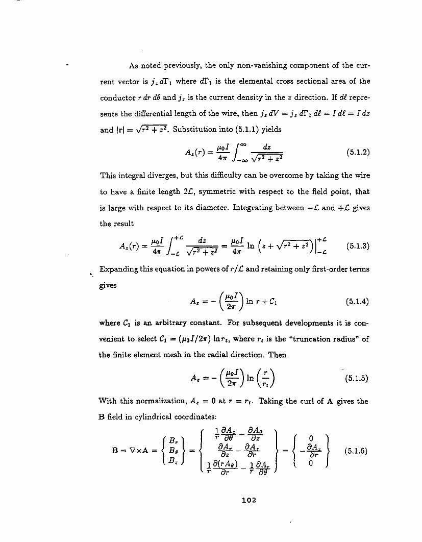
As noted previously, the only non-vanishing component of the cur-
rent vector is j.. dr1 where dr'l is the elemental cross sectional area of the
conductor r dr d6 and jz is the current density in the z direction. If de repre-
sents the differential length of the wire, then jz dV = jz FF1 dg = I de = I dz
and IrJ = _/r 2 + z 2. Substitution into (5.1.1) yields
Az(,) = _'°_/__ _/Jdz+z2 (5.1.2)
This integral diverges, but this difficulty can be overcome by taking the wire
to have a finite length 2_:, symmetric with respect to the field point, that
is large with respect to its diameter. Integrating between -£ and +/: gives
the result
(5.1.3)
Expanding this equation in powers of r//: and retaining only first-order terms
gives
Az = - \ _/_, + Cl (5.1.4)
where C1 is an arbitra.,T constant. For subsequent developments it is con-
venient to select C1 = (/_0I/2r) lnrt, where rt is the "truncation radius" of
the finite element mesh in the radial direction. Then
A, =- \ 2_ / _ _ (5.1.5)
With this normalization, Az = 0 at r = r_. Taking the curl of A gives the
B field in cylindrical coordinates:
B = VxA = Bo = _. = -"'0_r (5.1.6)
B: 10(rAo) 1 0.4_ 0_-"_ r
3.02

Itisseen that the only non-vanishing component of the magnetic flux density
is
c_A_ _oIBo = #o/-/e = - 0--_- = 2_r (5.1.7)
This expression iscalledthe law of Biot-Savart in the EM literature.
5.1.2 MAGNETIC FIELD WITHIN THE CONDUCTOR.
Again restricting our consideration to the static case, Maxwell's
equations in their integral flux form give
_cH.ds=_c#-iB.ds=_rj.ficdF (5.1.8)
where C is a contour around the field point traversed counterclockwise with
an oriented differential arclength ds and flcdF is the oriented surface element
inside the contour. The term for the electric field disappears in this analysis
because E = o. From before, it is known that the right hand side of (5.1.8)
is equal to the normal component of the current that flows through the
cross sectional area evaluated by the integral. In the free space case, this is
the total current that flows through the conductor. But in the conductor the
amount of current is a function of the distance r from the center. Again using
f to represent the total current carried by the conductor, and rc the radius
of the conductor, and assuming an uniform current density j z = I/(Trr_),
the right hand side of (5.1.8) becomes
j. fi dr = j:drl - _rr-2 dFi = I_--_2 (5.1.9)1 1
Evaluating the left hand side of the integral and solving for Bo gives:
27rr_ -I B8 : I r2- Be - ;ifrr_' 2_rr_ (5.1.10)
103

Comparing this equation with (5.1.5), it is seen that if # = #0 then B0 is
continuous at the wire surface r = re and has the value #0I/(2_rrc). But if
# # #0 there is a jump (_ - #o)I/(2_rrc) in B0.
The magnetic potential A= within the conductor is easily computed
by integrating -Be with respect to r:
_I7 "2
Az = 47rr_ + CI (5.1.11)
The value of CI is determined by matching (5.1.5) at r = re, since the
potential must be continuous. The result can be written as
Az=_ _ I- -#o in . (5.1.12)
The preceding expressions (5.1.5),(5.1.12)for Az can be verifiedas being
correct by substituting them directlyinto the Euder equation of (2.3.11).
5.2 FINITE ELEMENT DISCRETIZATION.
5.2.1 CONSTRUCTING EM FINITE ELEMENTS.
To deal with this particular axisymmetric problem a two-node "line"
finite element is sufficient. This provides the C ° continuity for As that the
variational formulation requires. In the following, individual elements and
element properties are indentified by the superscript (e). The two element
end nodes are denoted by the subscripts i and j. The magnetic potential A_
is interpolated over each element as
A_--- NA_ _) (5.2.1)
104

Here the row vector N contains the isoparametric finite elementshapefunc-
tions for A:. The elements of N are only functions of the isoparametric
parameter { which varies between -1 at node i and +1 at node j. The shape
functions are
N=½(1-_ 1+_) (5.2.2)
The shape functions are functions of the spatial variable r and the defining
relation between r and N is
r=N _)
A_ _) contains the nodal values for Az and are only functions of the time t,
A_e) = _1 (e)A (.r)
z 2
Substitution of these finite element assumptions into the previously derived
Lagrangian, Equation (2.3.9), and then into Equation (2.2.14), yields the
variational integral as the sum of elemental contributions R = ErR (r), where
f #<.,,r_4_.!.,T
The nodal values A_ ") are constant with respect to time because this is a
steady state problem. Therefore, the integration with respect to t disappears.
Taking the variation with respect to the element node values of A{ r) gives
5R(e)= gv(')fdV(e)SA(e)T{ 1�fir) ONTONo-'_0--7 A_z'r'j _ NTj!e) }
This can be written more simply as
KU(_)u (e) = p(_)
(5.2.6)
(5.2.7)
105

where
JV(,_)
Equation (5.2.7) is purposely written in a notation resembling the stiffness-
force equations of statics. K u(e) represents a stiffness matrix derived from
a potential energy variational formulation, u (¢) the nodal displacements and
p(_) repres'ents the external force vector. This form clearly illustrates that so-
lution and assembly techniques developed for finite element mechanics prob-
lems can be used to solve four-potential based EM field problems.
5.2.2 APPLYING BOUNDARY CONDITIONS.
The finite element mesh is necessarily terminated at a finite size,
which for this test problem is defined as the truncation radius r_ alluded to
in Section 5.2. In order to make the boundary integrals of R vanish, it is
necessary to look at the boundary integrals of (2.3.11). In the finite element
formulation, the discretized version of these integrals is
r OA= (1) r 8Az
where dl"2 is again d_dz, and Azl 1) and ,-zj represent the nodal values
for A: at r = 0 and r = rt respectively and numel is the total number of
finite elements. Simple observation shows that the first boundary integral
vanishes at r equal to zero. To make the other term vanish, the nodal value
for A= at r equal to rt can be constrained to zero. This is the essential
boundary condition used for this particular problem.
106
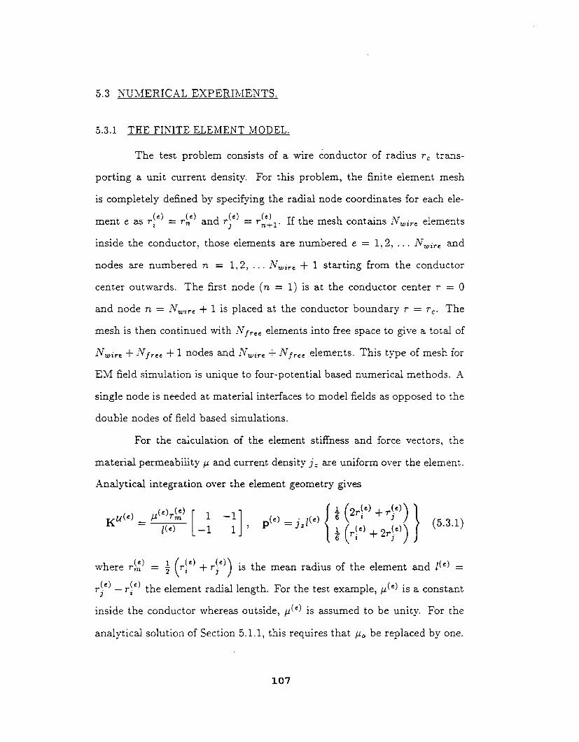
5.3 NUMERICAL EXPERIMENTS.
5.3.1 THE FINITE ELEMENT MODEL.
The test problem consists of a wire conductor of radius vc trans-
porting a unit current density. For this problem, the finite element mesh
is completely defined by specifying the radial node coordinates for each ele-
ment e as r! e) = r (e) and r (.e) _(e) If the mesh contains :Vwire elementsz ] -- rn+l.
inside the conductor, those elements are numbered e = 1,2,... Nwire and
nodes are numbered n = 1,2, ... Nwire + I starting from the conductor
center outwards. The first node (n = I) is at the conductor center r = 0
and node n = Nw_e + 1 is placed at the conductor boundary r = rc. The
mesh is then continued with !Y/tee elements into free space to give a total of
Nwi,-e+ iYfree+ I nodes and Nwire + IVf_e,elements. This type of mesh for
EM fieldsimulation isunique to four-potentialbased numerical methods. A
singlenode isneeded at material interfacesto model fieldsas opposed to the
double nodes of fieldbased simulations.
For the calculation of the element stiffnessand force vectors, the
material permeability > and current density jz are uniform over the element.
Analytical integration over the element geometry gives
-- ' i / (,)--9 (')_- 1 _ [r i + .ry )
1( -I-r_ )is the mean radius of the element and l(e)where r_ ) = 7 rle) *)
r(,) (e) the element radial length. For the test example,/_(') is a constantj --ri
inside the conductor whereas outside, #(_) is assumed to be unity. For the
analytical solution of Section 5.1.1, this requires that #o be replaced by one.
107

The longitudinal curent density is j= = I/(_rr 2) inside the conductor whereas
outside j_ vanishes.
The master stiffness matrix and force vector are assembled following
standard finite element techniques. The only essential boundary condition
requires setting the nodal potential on the truncation boundary to zero, as
explained in Section 5.2.2. The modified master equations are processed by
a conventional symmetric solver, which provided the value of the magnetic
potential at the mesh nodes. The magnetic flux density Be, which is constant
over each element, is recovered in element by element fashion through the
simple finite element approximation
B_e)_ aA: 0NA(e) - --z, .-zjOr -- Or z l_)" (5.3.2)
This value was assigned to the center of each element e for plotting purposes,
although it is a step function due to its C -1 continuity.
5.3.2 NUMERICAL RESULTS.
The numerical results shown in Figures 5.1 through 5.6 pertain to a
unit-radius conductor (r, = 1), with the external mesh truncated at r, = 5.
The element radial lengths, 1(e), were kept constant and equal to .25, which
corresponds to four internal and sixteen external elements.
The computed values of the potential A= are compared with the
analytical solutions of Sections 1.1.1 and 1.1.2. As can be seen, the agreement
between analytical and FE values is excellent. The comparison between
computed values of the magnetic flux density Be shows excellent agreement
108

except for the last element near the wire center, at which point the FE
approximation (5.3. i) loses accuracy.
Figures 5.1, 5.3, and 5.5 are for the case where #_,Te was I0.0, and
Figures 5.2, 5.4, and 5.6 are for the case in which #_T, was one, that is, the
same as the space surrounding the wire. Figures 5.1 and 5.2 show computed
and analytical magnetic potentials. The slope discontinuity at r = 1 in
Figure 5.1 and the jump in Be in Figure 5.3 are a consequence of the change
in permeability _ when crossing the conductor boundary. Figures 5.3 and 5.4
show the computed and analytical magnetic flux densities. Figures 5.5 and
5.6 show the computed and analytical magnetic flux densities in free space in
more detail. Note that Figures 5.5 and 5.6 for r > 1 are identical; this is the
expected result because as shown in Section 5.1.2, the free space magnetic
flux field depends only upon the current enclosed by a surface integral around
the wire and not on the details of the interior field distribution.
In summary, this finite element performed very accurately in the
example problem and converged, as expected, to the analytical solution as
the size of the elements decreased.
109
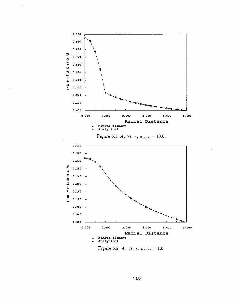
1.100
P0
te
n
tia1
0.990
0.880
0.770
0.660
0.550
0.440
0.330
0.220
0.110
0.000
0.000
\\
1.000 2.000 3.000 4. 000
Radial Distance
Finite Element
An_ytAcal
Figure 5.1:Az vs. r, #_ire = I0.0.
5.000
0.400
P0
te
n
tia1
0.360
0.320
0.280
0.240
0.200
0.160
0.120
0.080
0.040
0.000
0.000
\\
\
I I
1.000
\
I
2. 000 3.000 4.000
Radial DistanceFinite Element
Analytical
Figure 5.2: A_ vs. r, /_i,-_ = 1.0.
5.000
ii0

1.700
1.530
1.360
B 1.19o
1.020F
i o.,so /
° /1 0.6ao.
d0.510
0.340 '/
0.170
0.000 I
0.000
//
1. 000 2. 000 3. 000 4. 000 5. 000
Radial Distance
Finite Element
Analytical
Figure 5.3: Be vs. r, #_,ir_ = 10.0.Values shown on the interface r = 1 with
dark symbols have been extrapolated from element center values
to display the jump more accurately; this extrapolation scheme
has not been used elsewhere.
B
Fi
e
1d
0.170
0.153
0.136
0.119
0.102
0.085
0.0&8
0.051
0. 034
0. 017
0.000
/ \/ \
0.000
I I I I I I X I I
1. 000 2. 000 3. 000 4. 000
Radial Distance. Finite Element
o Analytical
Figure 5.4: Bo vs. r, #_ire = 1.0.
5.000
iii

B
F
ie
1d
1.700
1.530 _I1.360
1.190
i. 020
0.850
0.680
0.510
0.340
0.170
0. 000
0. 800 1.640 2. 480 3.320 4. 160 5.000
Radial DistanceFinite Elem_nt
o Analytical
Figure 5.5: Figure 5.3 for r > rc =1, _,-_ = 10.0, showing free space Befield in more detail.
0.170
0.136
0.119 -
F O.lO2
ei°"°ss ___1 0.068
d0.0SI
0.034 _S--_-_ o
0. 017
0.000 I I I _ [ i I I I
0 .800 1 .640 2 .480 3 .320 4 . 160 5 . 000
Radial DistanceFinit Q Element
Analytical
Figure 5.6: Figure 5.4 for r > rc =1, #_i_ = 1.0, showing free space Bo fieldin more detail.
112

5.4 SUMMARY.
In this chapter, the case of a simple one-dimensional infinite wire
is tested. To perform this test, the linear functional of Section 2.3 is dis-
cretized using standard FE techniques and appropriate boundary conditions
are determined. When the discretization is complete, it can be seen that the
governing equations are of a standard form and present no problems to the
use of standard FE solvers for linear systems.
Analytical solutions for the one-dimensional axisymmetric infinite
conductor are also derived in this chapter. Presented in this chapter are
graphs that compare results obtained from these analytical solutions and
from the FE model. The two solutions are in excellent agreement except at
the center of the conductor thereby validating the use of the four-potential
method for the determination of EM fields. Most importantly, th.e four-
potential method accurately predicts the B field across material interfaces
without any special boundary treatment, unlike the conventional field based
methods.
In the next chapter, the case of a two-dimensional problem with
similar boundary conditions and a -known current density is explored. The
extension of the four-potential method to the two-dimensional case is done
to offer further proof of the validity of this method for EM field analysis. It
is also performed in order to show the effect of the Lorentz gauge, as the
gauge effects disappear in the one-dimensional steady-state example.
113

THE CLEM2D FINITE ELEMENT
In this chapter, the four-potential FE element for axisymmetric two-
dimensional problems is developed. The new elements show the relatively
easy extension of the four-potential method through the use of Lag'range
multiplier adjunction to a broader class of problems. This element was tested
for two different geometries, a one-dimensional infinite conductor, and a
cylindrical "can" connected to two infinite feed wires on the top and bottom.
For both geometries, the current density j is known, and the static
charge density p is zero. The first geometry is the same as that of Chapter
IV, and is used to provide a check on the element calculations. The second
geometry is chosen to allow for a variation of B in more than one direction.
For this geometry, there is no analytical solution, but the results can be
examined to determine if they are physically realizable. For this reason, this
chapter begins with a discussion of the construction of the two-dimensional
axisymmetric finite element.
6.1 FINITE ELEMENT DISCRETIZATION.
In the previous chapter, the ungauged Lagran_an (2.2.13) is used
to construct one-dimensional axisymmetric finite elements. In the present
chapter, the four-potential method is extended to include two-dimensional
114

axisymmetric problems. In doing so, the basic four-potential does not nec-
essarily satisfy the gauge condition (2.1.10) a priori and consequently, the
gauged form of the four-potential (2.2.15) must be used.
6.1.1 CONSTRUCTING EM FINITE ELEMENTS.
For the finite element discretization of the two-dimensional case,
quadrilateral a,xisymmetric elements defined by their geometry on the r-z
plane are constructed. These elements are isoparametric with corner node
points only. Additional construction details are provided in a later section
of this chapter.
In the following, individual elements and element properties are
again identified by the superscript e in parentheses. The element nodes
are locally numbered i = 1,... n, where n is the number of corner nodes
(n = 4 for quadrilaterals). The magnetic potential components, A,-, Ae and
Az = NA_ e)
A: are interpolated over each element as
(6.1.1)
Here the row vector N contains the isopaxametric quadrilateral shape func-
tions, which are only functions of the radial and longitudinal coordinates r
and z
N- ( N,(r,z) Nz(r,z) N3(r,z) N4(r,z) ) (6.1.2)
and column vectors A ('), A (e), and Ai e) contain the nodal values of At, As
and Az respectively, which are only functions of the independent variable t
A(_e)=(A,-l(t) Ar_(t) Ar3(t) A,-4(t)>
A_e)=(A81(t) Ae2(t) Aea(t) A84(t)>
A_ e) = (A.-l(t) A,2(t) A_s(t) A:4(t)>
(6.1.3)
115

where, as in the one-dimensional time-independent case, the nodal values
for A (e), A(ee) and A! e) becomeconstants. Substitution of the above as-
sumptions into the previously derived Lagrangian, Equation (2.4.1), and
integration over the volume of the elementyields the variational integral as
a sum of element contributions R = EeR(e),where
R(e) =
+ A_e)T 0N0z7"0N0z A_e))
0 CONA(e)'_ }
(6.1.4)
and V (_) again denotes the volume of the element. Varying the above equa-
tion with respect to the element node values A_ e) produces
_R(6._'))= Jr(,,/ dv(')6A(:)_/A-(_(o)( _NTaNozOzA(°)ON r ON "_
Oz Or A(e) /
(6.1.5)
Taking the variation of (6.1.4) with respect to A (e) gives
ON TON (e)'_ _ NTj_e) 1+ Oz -O-fA° ) )
(6.1.6)
116

and taking the variation of (6.1.4) with respect to A(=_) produces
/t 8N r ON ,_,'_6R(6A(_))" = ,v(°)fdV(_)6A(_)T" 7 7yl kcONTor 8NA('_)0r" Or 0-7 A_ ')
aNT NTj_,) }+ )_g 8z
(6.1.7)
The variation of (6.1.4) with respect to the last independent variable Ag is
0 ON (_+--A ) (6.1.8)
To facilitate a more compact formulation, the introduction of the following
matrix notation is used for the stiffness matrix
K u(e) =
K(e) A,.A,. 0 K(e) A,.A, K(e)A,A9
K(e) AoAo 0 0
K(e)A,A, K(e)A=A9
symm. 0
(6.1.9)
where
K (_)A.A. = .Iv(.)f dV(_) ( 1 ON T )
ON
_(_) Oz -&z
K(_)A'A' =fdV(e)1 (( 10(aV(,) --#(e) _ rN T)) (1 0_r (rN)) 0NTaN)+0z 0z
K (') A,,_, [ dV (_) Ag o-NTJV(=) Oz
1 ONTON' IK(e)A,A_
ON T ON t
)Oz Or
(6.1.10)
117
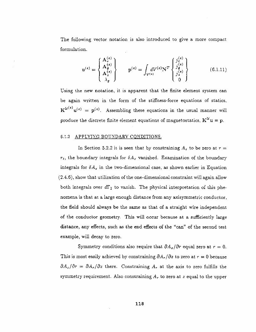
The following vector notation is also introduced to give a more compact
formulation.
A (e)
u (_) = A!_)
A9
?)}j_)
0
(6.1.11)
Using the new notation, it is apparent that the finite element system can
be again written in the form of the stiffness-force equations of statics,
Ku(_)u (_) = p(_). Assembling these equations in the usual manner will
produce the discrete finite element equations of magnetostatics, KUu = p.
6.1.2 APPLYING BOUNDARY CONDITIONS.
In Section 5.2.2 it is seen that by constraining Az to be zero at r =
r,, the boundary integrals for 6A_ vanished. Examination of the boundary
integrals for 6A, in the two-dimensional case, as shown earlier in Equation
(2.4.6), show that utilization of the one-dimensional constraint will again allow
both integrals over dF2 to vanish. The physical interpretation of this phe-
nomena is that at a large enough distance from any axisymmetric conductor,
the field should always be the same as that of a straight wire independent
of the conductor geometry. This will occur because at a sufficiently large
distance, any effects, such as the end effects of the "can" of the second test
example, will decay to zero.
Symmetry conditions also require that cOAz/Or equal zero at r = 0.
This is most easily achieved by constraining OAr/Oz to zero at r = 0 because
cOA,/Or = cOAr/Oz there. Constraining Ar at the axis to zero fulfills the
symmetry requirement. Also constraining A_ to zero at z equal to the upper
118

and lower mesh boundaries will make the boundary integralsof Equation
(2.2.2)disappear.
The application of these boundary conditions removes the rank de-
ficienciesof the assembled master stiffnessmatrix. They are not the only
boundary conditions that will work, as examination of Equations (2.4.2),
(2.4.5)and (2.4.6)show, but they are the easiestto derive,being based upon
simple physical and mathematical arguments. These are the boundary con-
ditionsthat are used for the two-dimensional examples presented herein.
6.2 NUMERICAL EXPERIMENTS.
6.2.1 THE FINITE ELEMENT MODEL.
The finite element formulation described in the previous section has
been applied to the solution of the two test examples described at the begin-
ning of this chapter. Both problems are treated with quadrilateral elements.
Each quadrilateral element has four corner points and one interior node.
_(e) and _(e) AtThese nodes are defined by their radial and axial positions r, z i .
each corner i, there are three degrees of freedom, namely Ari, Aoi, Az,. From
these values, the potential components are interpolated with the standard
bilinear shape functions, which provide the C ° continuity required by the
variational formulation. The centroidal node carries no physical significance
and is used solely to provide the extra degree of freedom assigned to the
Lagrange multiplier Ag(e) Thus each quadrilateral element has 4 x 3 + 1 =
13 degrees of freedom.
For the calculation of the element stiffness and force vectors, it is
assumed that the permeability #(e) and the current densities are uniform over
119

each element. The desired stiffness matrix and force vector are calculated
by numerical quadrature using Gauss formulas. The portion associated with
the potentials is always evaluated with the 2x2 rule. On the other hand,
three different schemes were tried on the entries associated with Ag:
Fall Integration. The same 2x2 rule as for the potentials is used.
Selective Integration. A one-point rule is used for K (_) and K (e)A, A9 A, X_ "
Zero In*egra*ion. The effect of Ag is ignored by omitting the integration of
the associated terms and placing ones on the diagonal. This numerical device
effectively forces Ag = 0, and thus "releases" the gauge constraint.
6.2.2 ASSEMBLY, SOLUTION AND FIELD RECOVERY.
The master stiffness matrix and force vector are assembled follow-
ing standard finite element techniques. The boundary conditions are set as
explained previously. The modified master equations modified for bound-
ary conditions are processed by a standard symmetric skyline solver, which
provides the value of the potentials at the mesh nodes.
The physical quantities of interest are not the potentials but the
magnetic flux density B. This is calculated by discretizing the curl of A.
Since 0A/c3# = 0, the magnetic fields become, after discretization,
ON A(_) ON A(e)Bo = -_ _ -W z . (6.2.1)
Bz 1 cO(rN A(, )r(e) Or 0
The nodal values for B are obtained by evaluation at the Gauss point followed
by extrapolation to node locations. The average of these quantities is also
reported as the centroidal value. As discussed below this value is found to
120

be more accurate than interelement-averaged node values. Consequently the
centroidal value isused to report results.
For both testproblems, the magnetic permeability #(e)= #wire was
constant insidethe conductor whereas outside itthe free-space permeability
#(*) = #/,._ was assumed to be unity. The current densitieswere assumed
to be uniformly distributed and consequently were calculated by dividing
the assumed total current flowing through the conductor by the total cross-
sectionalareas of the conductors.
6.2.3 PROBLEM 1: A CONDUCTING INFINITE WIRE.
The first test problem is identical to that reported in the previous
chapter with a one-dimensional axisymmetric discretization. ' As shown in
Figure 2.1, it consists of a wire conductor of radius rc transporting a total
current of I = 1 ampere in the z direction. This current was assumed to
be uniformly distributed over the wire cross section. For this problem one
layer of quadrilateral elements in the z direction, extending from z = 0
through z = d, was sumcient; here the distance d was chosen arbitrarily.
The radial direction is discretized with Nw_,-, elements inside the wire and
NSr** elements outside the wire in free space. The mesh is terminated at a
"truncation radius" r, >> rc where the potential component Az is arbitrarily
set to zero. Other boundary conditions are A,. = 0 on the nodes at r = 0,
z=0andz=d.
The results obtained with r, = 5re, Nw,_, = 4 and -J¥._,-e, = 10 for
the potentials are identical to those reported in the previous chapter, thus
providing a check on the element calculations. The same results were also ob-
tained with the three integration schemes noted above for the As term, which
121

verifies that the Lorentz gaugeconstraint (2.1.10) is automatically satisfied
by the finite elementshapefunction for one-dimensionalmagnetostatic fields.
The computed magnetic flux density B# at node points was not as
accurate ascould be expected,generallybeing too large, especiallyat r = 0.
The centroidal values_on the other hand, were considerably more accurate
as regards matching analytical results. Thus for the secondproblem field
values at the element centroids are reported. The extrapolation of B to
nodal locations is a disadvantageof the four-potential variational approach.
Field basedformulations cancompute the value of the B field directly at the
nodal locations while the four-potential method cannot.
6.2.4 PROBLEM 2: A CONDUCTING HOLLOW CAN.
The second test problem, shown in Figures 6.1 and 6.2, brings two-
dimensional features. It is a hollow conducting cylindrical :'can" with infinite
feed wires connected to the center of its top and bottom faces. These wires
carry a total current of I = 1 ampere in the +z direction; this current
was assumed to be uniformly distributed over the varying cross sections it
traversed. For the ends of the can, it was assumed that the current flowed in
the 4-_r direction, forcing J0 to be zero. For the areas where the feed wires
join the " "can , and the corners of the "can", it was assumed that the current
turned ninety degrees and was uniformly distributed. This assumption is
unrealistic physically, but warranted for the mesh used in this test problem.
The mesh choice is discussed below. The wire radius rc and the can wall
thicknesses were assumed to be identical.
Because of the symmetry of the problem it is sufficient to model only
the upper half z > 0. The results presented here were obtained by using a
122

* current I
radius rC
.hickness rc
Figure 6.1: Cross-section of two-dimensional axisymmetric case.
Cross-section taken through z axis.
123

l-i
o,.., o
Cr_
C_
0
0
0
e...o
(I)
0
P__
_D
I--.f *

25 × 25 element mesh of square elements. Within this mesh, the wire as "?-ell
as the can walls were modeled with only one element across the radius or
thickness,respectively.
The regular mesh indeed represents an "overkill"for the free space
while itisinsuflZicientlyrefinedto capture fielddistributiondetailsinsideand
near the conducting material. This mesh was actually chosen to conform
to limitations of the three-dimensional plotting functions of the software
pac "t_ge Mathematica.
The problem was run using full, selective and zero integration
schemes for the A9 freedoms. The magnetic permeability #f_e in the free
space outside the conducting material was chosen as unity. For the conduct-
ing material two different values for the permeability # = #wire were tried:
1.0 and 10.0; the latter to check whether flux jump conditions were auto-
matically accommodated by the potential formulation. Selective results are
reported graphically in Figures 6.3 through 6.8. Figures 6.3 and 6.4 show
the magnitude of Be for #_i,-, = #.h-ee = 1 obtained for the full and zero
order integration schemes, respectively. Figures 6.5 and 6.6 show these re-
sults in contour plot form. Figures 6.7 and 6.8 correspond to #wi,-, = 10 and
show the magnitude of Be from different viewing points. A discussion of the
results follows.
The full integration scheme for As performed well outside the con-
ductor. Results were compared with those of the analytical solution for the
infinite straight wire (the first test problem) to determine whether they were
physically reasonable. As r becomes large compared to the can cross dimen-
sion (towards the outer radial edge of the mesh), the answers agreed. This
is the expected behavior, because as r goes to _, the general axisymmetric
125

problem should behave as an infinite straight conductor. As one moved to-
wards the top of the mesh, the solution again approached that of an infinite
wire as can be observed in Figures 6.3 through 6.8. This behavior is expected
because as we move p_lel to the wire in the z direction, the effects of the
current in the can ends should tend to zero and the only far-field effects
should be from the total current. The results for the magnetic field within
the feed wire were not accurate as it did not vanish for r = 0; this behavior
was due to the use of only one element across the radius and the fact that
only centroidal values are reported as noted above.
The selective integration scheme gave answers of the same general
shape as the full integration scheme, but they only agreed to one or two
significant digits; these results are not shown here as they are hard to dis-
tinguish in plots. The zero integration scheme (which in fact releases the
Lorentz gauge coupling), gave solutions for the field that were larger than
expected at the conductor boundary and a physically unrealizable field in-
side of the _'can". This field grows shm'ply as the can axis is approached, as
shown in Figures 6.4 and 6.6.
126
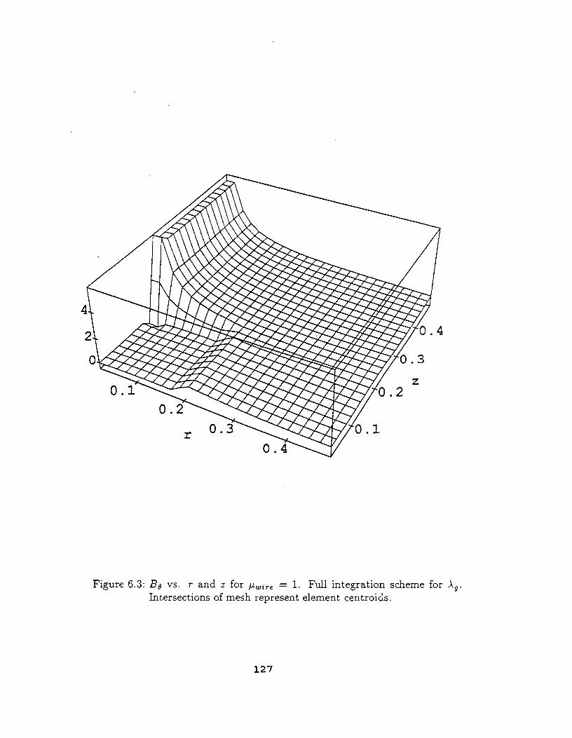
0.2
r0.3 0.I
0.3
Z
0.2
Figure 6.3: Bo vs. r and z for #wire = 1. Full integration scheme for Ag.
Intersections of mesh represent element centroids.
127

6_
4
2
C 0.3
z
Figure 6.4: Be vs. r and z for #,_,,-e = 1. Zero integration scheme for Ag.
Intersections of mesh represent element centroids.
128

25 .z
20-
15-
5-
I I
5 I0, , ir
15 20 25
Figure 6.5: Contour plot of Be vs. r and z for #_i,-_ = I. Full integration
scheme for Ag. Numbers on axes represent the number of element
centroids traversed from the center of the "can". Each element is
.02 × .02 square. All contours are equally spaced and range fromminumum to maximum values of the field.
129

25 .z
15
10
III
!I
II
!jj)
t10
1 I I E5 15 2O 25
Figure 6.6: Contour plot of Bo vs. r and z for #wi,-, = 1.0. Zero integration
scheme for A 9. Numbers on axes represent the number of element
centroids traversed from the center of the "can". Each element is
.02 x .02 square. All contours are equally spaced and range fromminumum to maximum values of the field.
130

60-
4C
2C
(
0.I
0.2
0.3r
0.3
Z
0.2
Figure 6.7: Bo vs. r and z for #wire = 10. Full integration scheme for A_.
Intersections of mesh represent element centroids. Note sharp
field jumps on conductor surfaces.
131

40
a 20"
O"
0.4
•
Z•
0 .4
D.3
r
0 .i 0 .i
Figure 6.8: The same case as Figure 6.7 shown from a different viewing point
to emphasize how Be fails to go to zero as r approaches zerobecause of the coarse conductor discretization.
132

6.3 SUMMARY.
The results of the CLEM2D finite element show that the four-
potential variational principle can be applied to a broader class of prob-
lems than the simple one-dimensional axisymmetric conductor. Although no
analytical solution is available for direct comparison, the physical behavior
of the numerical results strongly suggest that they are accurate. The only
point where the results are inaccurate are within the conductor itself. A finer
mesh grading within the conductor can solve this problem, as results o£ the
previous chapter illustrate.
The only truly unrealistic assumption about the second test prob-
lem was the assumption of the current density distribution. A physical cur-
rent mill in general not make a ninety de_ee turn and remain uniformly
distributed. To address this problem, the CUPLE series of elements was
developed. Given a known current I, these elements can determine the dis-
tribution of the current density j as well as the B and E fields. These finite
element models are the subject of the next chapter.
133

THE CUPLE1D FINITE ELEMENT
In this chapter, the four-potential finite element for one-dimensional
problems with an unknown current density vector is developed and tested
for two examples. Both examples possess the same circular-wire geometr_,
shown in Fibre 2.1, no static charge density (p = 0), and a known current
I in the positive z direction. In the first example, all elements have equal
conductivities. This example gives the same type of fields encountered in
Chapter V and is used to verify the accuracy of computed solutions. For
the second example, the element conductivities are allowed to differ. An
analytical solution to this problem exists and is compared with the numerical
solution.
7.1 ANALYTICAL SOLUTION TO THE TEST PROBLEM.
7.1.1 MAGNETIC FIELD WITHIN THE CONDUCTOR.
The Euler equation for $Ac of Equation (3.1.11) states
I= Jfr dr'lj, (7.1.1)1
This is the law of current conservation. For the examples presented here, it
is assumed that jz and w are simple step functions where w is known and jz
134

is unknown. Using these assumptions, (7.1.1) becomes
n_ TO. e _
dr(e)j_ (_) (7.1.2)I ----- __,(_)
e=l
where a superscript letter or number in parentheses denotes the element
number and numel is the total number of elements. The Euler equation for
5n0 of Equation (3.1.11) over each volume disappears because j_e) and a_(_)
are step functions. If _ is constrained at r = 0 and r = re, the set of surface
integrals for 5_0 of (3.1.11) do not vanish and produces the following set of
nurnel - 1 equations relating the j,(e)'s
j_(e)w(_) = j (e+l)w(e+l) (7.1.3)
Insertion of (7.1.3) into (7.1.2) gives
n lt'rll _ l
I = aJ(1)j_ (1) E fr(o_e=l
dl"(e)a, ,(e) (w(1)) -1 (7.1.4)
The above is used to determine j:(_), and this value is then used with (7.1.3)
to solve for the remainder of the undetermined jz (e)'s.
Equation (5.1.8) states
SFor this example, # is a constant over the volume of the conductor. This
assumption is discussed at the beginning of Chapter IV. For the one dimen-
sional case, the contribution for each j(e) using (7.1.5) is
Be (e) = -_j_(e)r (7.1.6)
135

where ri-C_)< r < rj-Ce)and ri-(e)and rj-(_)represent the inner and outer bound-
aries of jz(_). For r = r!_) Be (e) is zero. Using the principle of linear
superposition, the totalB fieldis
Be= _ \_=ir(e)<r <r_ _)i
(7.1.7)
The value of Az (')is computed by integrating(7.1.6)over r and taking the
negative of the answer, which is
A.(_).= - / B_d_= -,jr (_)_4 + Co (7.1.S)
where Co is again an integration constant. For _(e) equal to zero, Co is chosenr i
as zero. To ensure the C ° continuity specified for A_ by the four-potential
variational principle, Az,!2) must equal Az_ 1) when both are evaluated at
rj(i) = ri-(2)' This requires that for A=j = A= i , Co equal -# r /4j= (i).
The value of Co for each region where j(_) changes can be evaluated in a
similar manner. Doing so will give the following expression for A,
(') -(') (7.1.9)r i < r <_ rj
136

7.1.2 THE FREE SPACE MAGNETIC FIELD.
Using Equations (7.1.5)and (7.1.1),the expression for Be in the free
space outside of the conductor is
#of2_0 = --
2_r
The value for the potential.42 is
Az - - / Bodr -
(7.1.10)
#of Inr + Co (7.1.11)27r
Use of Equation (7.1.9) to determine Co gives the following expression for A_-
A: = - 2-_x #° in + _t (7.1.12)
The above result differs from the previous solution of (5.1.5) by a
constant. This is not surprising because, in the one-dimensional case, A is
not unique and is determined solely by the boundary conditions. For the
example of Chapter V, A is constrained to zero at rt. For this example, A
is constrained to zero at r equal to zero. For a one-dimensional bulk super-
conductor using the London gauge, A must vanish at r = 0 as discussed in
Section 3.2.1. Because of this boundary constraint on a superconductor, A
is also chosen as zero at r = 0 for the one-dimensional current density pre-
dicting case. This choice is made so that numerical coding that implements
both elements to model the phase transition of a superconductor will require
only one set of boundary conditions for A. The consequences of this choice
are discussed in the subsection on applying boundary conditions.
7.2 FINITE ELEMENT DISCRETIZATION.
137

7.2.1 CONSTRUCTING EM FINITE ELEMENTS.
To deal with this particular axisymmetric problem, the two-node
"line"finiteelement isagain sufficient.Individual elements and theirconsti-
tutive properties are denoted by a superscript (e). The element end nodes
are alsodenoted by the subscripts iand j again..4z and teeare interpolated
over each element as
Az = NA_ _) _e = N_ e) (7.2.1)
The row vector N contains the isoparametric shape functions for the inter-
polation of A_ and _e- The elements of N are only functions of the spatial
coordinate r. A_ _) and _) contain the nodal values for A= and _e and are
only functions of the time t, and for the time-independent problem studied
here, become constants with respect to time. Substitution of these finite
element assumptions into the previously derived variational functional of
Equation (3.1.10) gives
__- --A_, - __e" "w'" 1_" _(¢)A(_)TNTJ v_,) 2_(') Or O'-r/ J= "
- .-o Jr '>
+ (z-/"4t'>' )(7.2.2)
where dF2 and dFi are again dSdz and rdrd8 respectively. Variation with
respect to A! _), _), Ac and j(¢) produces the following expression for the
138

elemental stiffnessmatrix
K(e)AA g(e) Aj 0 0
..(e)K(e)_j I_'_; ) K(e) J ,¢ "_"jxo
0 K (_)r 0 03_
0 K (e) Tj;,_ 0 0
(7.2.3)
where
Xii e)o.,(e)2 (7.2.5)Jr(,) Jr ')
av(:) _r (rN) (7.2.6)
The above expression for K u(_) is not complete because it neglects contri-
butions to K(e)j,_ from the boundary integral over aft'2. The discussion of
this contribution is deferred to the subsection devoted to the application of
boundary conditions. Following the notation of previous chapters, u (O is
expressed as
{ }u(*)= Jl;, )) (7.2.7)
£¢
It is important to note that £¢ is a global degree of freedom. This condition
must be met when the elemental matrices are assembled to form the master
stiffness matrix.
_(¢) with respect to the independentTaking the second variation of ._p
variables produces the tangent stiffness matrix K, which is identical to K u(¢) .
This occurs because K u(_) is only a function of the radial coordinate r and
139

not the independent variables. This fact is important when non-linear solu-
tion techniques, such as the corrective Newton-Raphson method, are used for
the thermally coupled superconducting problem. To use the non-linear solu-
tion techniques, the tangent stiffness matrix is required, and the equivalency
of K u(e) and K means that K u(e) may be used in the normally conducting
portion with no modification.
7.2.2 APPLYING BOUNDARY CONDITIONS.
As mentioned in the previous subsection, K u(¢) is not complete be-
cause the boundary integral term over dF2 is not evaluated. The expanded
form of this term is
I
2_HrNlaoi(1) _'(1) £(1)[]z. rl 1) __ Z_TI_I TI¥2t_O j(numel+l) _j( numel )Jz'(numel) r! I)
(7.2.8)
where H is the height of the element, nurneI is the total number of elements,
N1 and .hr2 are the shape functions of N for the two-node "line" finite element
and the superscript terms in parentheses represent an element number again.
(1)Taking the variation of(7.2.8) with respect to the independent variables _ei ,
:(nuraet)(nurnel) j!l) and ]_ and evaluating at the specified values for r givestCOj
T, (x)¢ (1) .(1)j(1) (,_,n,0 .(--,,_*0,.(-,_,0_(,,m,07rl"lr i o_oi _ -- 2_Hrj 6_j _, j,
"_xa ri _Oi t_ --2 Hrj _j _ vjz
(7.2.9)
There remains in R (_) a volume term that contains _;_e) as an independent
variable. The variation of this term with respect to j_) and _) produces
(7.2.10)
_j_')K (¢)j_a_') = 0
(e)T-.'(e) T :(e)
_0 IX j,cJ z = 0
140

Evaluation of K(_)j. for a two-node element gives
-(_) -(_)> (7.2.11)K(e)j,¢ = 27rHaJ (e) ( -r i rj
Using this equation, 8j!_)K(e)j_ _e) for e = 1 and e = nurnel is
_jz(1)'r.,-(1) (1) _j!l) {,)7r.B,a.,,(, ) (_7. i Tj }r'i,, _0 = _(1) _(1) ) _])
6J(Z""_O""(""""O_i,, no('_"m_O
= 8j!.u_O {2,.rH_(n,,m_0 ( _(,-_m_0 (,_,,_t) ) (,-.,_0- --i 5 j
Addition of the third and fourth terms of (7.2.9) to the above gives
(_:(1)K(1)JzJ'cl¢o(1) = 6j_1) {27rHw(1) (0 r (3)J )_o(1)}
";( numet)14"( numet) _'( numel) (7.2.13)J z _'"j_ "_0
= . --r i 0 >
5tc(e)TK(e)T 4(e)Evaluation of 0 j_j_ at e = 1 and e = nurnel and the addition of
the first two terms of Equation (7.2.9) reproduces the transpose of the above
results.
These results have three consequences. The first is that for e = 1
and e = numel, zeros should be inserted in the appropriate positions of the
stiffness matrix to account for the effects of the boundary integral over F2.
Performing this operation creates a rank deficiency in the master stiffness
matrix. A solution to this problem is to insert a one (1) on the diagonal
elemefit of K at the appropriate degrees of freedom and to then constrain
_ (1) and (,_,,,_et)oi _oj to zero. This is easily accomplished and causes no ma-
jor difficulties for finite element analysis. Second, we now have a system
of nurnel - 1 equations for _0. The physical significance of this is that a
(7.2.12) _
141

Lagrangian multiplieris assigned to each of the boundaries in the conduc-
tor where aJ may change, thereby ensuring the verificationof the Max_vell
equation _xE = 0. Again, no difficultiesensue and the formulation still
matches the actual physics of the problem. Third, there are now nurnel - I
equations relating the nurnd degrees of freedom associated with the j_e)'s.
The latterconsequence isthe most important because itshows that the con-
stralntAc is necessary to remove the rank deficiencyof the master stiffness
matrix associated with the j_)'s.
As mentioned earlier,the boundary condition on -4z has been
changed so that the interiornode of the conductor is constrained instead
of the truncation node. The appropriate boundary integralof (3.1.11)is
r 0.4: r OAz_2'Az {-fi -_v } r - _2,Az {-fi -_r } o (7.2.14)
As assumed in Section 7.1.1 and at the be_nning of Chapter IV, # is assumed
to be constant for the examples of this work.
to produce the following result
Equation (5.1.8)is then used
IIe= _#-10Az _ I (7.2.15)oqr 2_rr
A minimum amount of algebra and the above relation changes (7.2.14) to
fr I ] = -H I6A,2 rt r t
(7.2.16)
where the first integral is again allowed to vanish at r = 0.
In Chapter V, the truncation node at r = rt is constrained to zero.
This will produce a reaction force at that node of magnitude HI because
the imposed constraint is an essential boundary condition. On the other
142

hand, at the degree of freedom associated with Azl 1) there is no boundary
force because the boundary integral vanishs there. In the case presented
in Chapter V, the reaction force at the last degree of freedom for A= was
not necessary for the analysis of the example problem. This information
is needed here for the determination of the new boundary forces. If A. is
constrained to zero at r equal to zero, a reaction force of -HI is produced
at the degree of freedom associated with A:I z). This situation is analogous
to changing the end constraint for a one-dimensional bar with a point force
on the free end from one end to the other.
For this example, it is necessary to achieve the same loading that
(n,Lme0was exhibited for the example of Chapter V when A.j was constrained.
This loading will produce the same B fields but different values for A. Again,
it is easier to visualize the rational for the above statement by again exam-
ining the example of a one-dimensional bar again. For a one-dimensional
bar, this would require that the same stresses be produced in the bar for
the different set of displacements produced by constraining first one end and
then the other. The validity of this comparison is shown by an examination
of(5.2.1). The expression for K u(e) is the same as that for a one-dimensional
FE "bar" element with a linearly varying cross-sectional area. Young's mod-
ulus has been replaced by 1//_ (*), and the cross-sectional area is denoted by
r_ ). For the forcing vector p(*), we see that j: is a uniformly distributed
constant loading force.
For our problem, to maintain the same boundary forces that are
( nurnel)exhibited when .._y is constrained, a reaction force of -HI is added
at this degree of freedom, and another reaction force of HI is added at the
143

first degree of freedom for A... The second force is added to cancel the force
of -HI produced when _ (1) is constrained.
The above reaction forces can also be used for a one-dimensional
superconductor. The forces are the same because variation of the terms in
AF associated with Az will produce boundary integrals that are identical
to those in Equation (7.2.14). The use of (5.1.8) to determine an analytical
expression for these integrals will still apply because the integral on the
right hand' side of (5.1.8) requires only the knowledge of the current I within
the conductor and not its distribution. The only limitation for the correct
determination of the boundary integral of (7.2.14) is that r >_ re.
Finally, one more reaction force appears from the variation of R_ e)
with respect to Ac. This force has a magnitude of -I and is applied at the
degree of freedom associated with A¢. Consequently, only three non-zero
values appear in the global external force vector p.
7.3 NUMERICAL EXPERIMENTS.
7.3.1 THE FINITE ELEMENT MODEL.
The finite element formulation derived in the previous section has
been applied to two test problems described below. Both problems are
treated with one-dimensional axisymmetric elements. Each of these "line"
elements has two end nodes and a common shared glodal node. These nodes
-(*) and _(e) Each end node has threeare defined by their axial positions r i ,j .
degrees of freedom. The first degree of freedom corresponds to _(e) and
the third degree of freedom corresponds to A (e). From these values, the
components of the magnetic potential and the Lagran_an multiplier ne are
144

interpolated with the standard linear shape functions, which provide the C °
continuity required by the variational formulation. The second degree of
freedom corresponds to j_e)on the interiornode while the exteriornode has
no independent variableassociated with iton the elemental leveland is con-
sidered "empty". This second degree of freedom has no physical significance
and ](:_)is carried on the interiornode so that an extra node per element
does not have to be injected to account for this independendent variable.
This scheme is used because it matches the format of the STEPID finite
element which carriesno injected interiornodes. The use of this scheme
makes downstream coupling of these elements, when modeling the complete,
coupled EM-thermal problem, more computationally efficient.All entriesin
K u(e) associated with the "empty" degree of freedom are assigned the value
of zero. The common shared global node isinjected at the end of the finite
element mesh. Itcarriesno physical significanceand isused solelyto provide
the extra degree of freedom assigned to Ac. Consequently, each element has
2 x 3 + 1 = 7 degrees of freedom.
For the calculationof the element stiiTnesses,itisassumed that the
permeability #, the resistivity w, the permittivity _ and the current density
j= are constant over the element. The desired stiffness matrix is calculated
by numerical quadrature using a two point Gauss rule. As mentioned at the
end of the preceding section, only three non-zero values appear in p and the
calculation of p(e) is not necessary.
145

7.3.2 APPLYING BOUNDARY CONDITIONS.
The finite element mesh is necessarily terminated at a finite size.
For the two test problems, the outer radial end of the mesh is defined as the
truncation radius r = ft. The outer radial end of the conductor's mesh is
defined as the wire radius rc. Since current is only carried in the conductor,
the degrees of freedom for j= between rc and rt are constrained to zero.
Similarly, the degrees of freedom for _;0 between rc and rt are also constrained
(1) (numel)to zero. The degrees of freedom corresponding to _0i and _0j are
also constrained to zero as explained in Section 7.2.2. A= is constrained to
zero at r equal to zero and HI is injected into p at the degree of freedom
,.4 (nurnel)corresponding to A: i(1)- At the degrees of freedom corresponding to ,,:j
and ,kc, -HI and -I are injected into p. The use of the seven degrees of
freedom format for each finite element results in a rank deficiency of one
for the assembled master stiffness equations. This occurs because there are
only nurael j(*)'s but the elemental degree of freedom format used produces
nurnel+ 1 equations when assembled. The last element only contributes zeros
to the master stiffness matrix for the second degree of freedom of the external
(j) node. To remove the rank deficiency, the second degree of freedom on
the outer node of the last element is constrained to zero.
7.3.3 ASSEMBLY, SOLUTION AND FIELD RECOVERY.
The master stiffness matrix is assembled following standard finite
element techniques. During the assembly, the elemental entries for _011) and
_o_ nu''et) are modified as discussed in Section 7.2.2. The external force vec-
tor is assembled by injecting its three non-zero entries as described in the
146

previous section. The remainder of the boundary conditions are set as ex-
plained previously. The modified master equations, modified for boundary
conditions, are processed by a standard symmetric skyline solver, which pro-
vides the value of A: and _0 at the mesh nodes, A, at the injected node, and
the mean current density over each element.
As in previous chapters, the physical quantity of interest is the mag-
netic flux density Be. The finite element approximation of Equation (5.3.2)
is used again. However, this time Bo is plotted as a step function to avoid
the extrapolations necessary to determine the value of Be at re.
The ability of the potential formulation to model the discontinutiy in
the B field at a conductor/free space has already been established in previous
chapters. For this reason, in both test problems # and _ were set equal to
one (I) inside the conductor and in the free space surrounding it. The first
test problem set all of the oJ(e) 's to one, and the second problem set each _(e)
to equal the inverse of the element number (i.e., cr(e) equaled the element
number).
7.3.4 PROBLEM I: EQUAL CONDUCTIVITIES.
The firsttestproblem isidenticalto that reported in Chapter V and
possesses a one-dimensional axisymmetric geometry. As shown in Figure 2.I,
itconsistsof a wire conductor of radius rc transporting a totalcurrent I = 1
ampere in the positive z direction.The elements were given a unit thickness
in the z direction. The radial directionis discretizedwith Nwi,-e elements
insidethe wire and 2¥/_eeelements outside the wire in freespace. The mesh
is truncated at a ':truncationradius" r,. Boundary conditions were set as
previously defined.
147

The results obtained with r, = 2re, N,_i,-e = 20, Nir,,= 20 for the
potentials differed from those generated by the previous EM finite elements
of Chapter V by a constant, as expected. These results are shown in Figure
7.1. They illustrate what appears to be an almost exact matching of the
computed solution to the analytical solution. Analysis of the data values
shows that at r equal to zero the error is about 33 per cent. The error
declines rapidly to .2 per cent at rc and even further to .08 percent at rt.
This error is attributed to the relatively coarse mesh used for the example
problem.
Figure 7.2 shows the results obtained for the computed current den-
sity. The result obtained is lower than the true value by less than one ten
thousandth of a percent, thus providing a check on the element calculations.
Because these results were so close to the exact solution, they were plotted
as a series of points, rather than a line, so that they could be distinguished
from the exact solution.
Figure T.3 shows the results obtained for the Be field. To evaluate
how closely the finite element solution matches the exact solution, it must
be observed where the analytical solution intersects the tops of the finite
element "steps". For an exact matching, the analytical solution will intersect
the middle of the "step" tops. Although dii_cult to see, at r equal to zero,
to approximately r equal to .1, the exact solution moves right of center on
the "steps". This means that the computed solution is larger than the exact
solution. The error in the computed solution ranges from 33 percent at the
center of the conductor to 4.6 percent at the conductor boundary. Outside
of the conductor, the error trailed off to .02 per cent. The high error at the
center of the conductor is due to the relatively coarse mesh discretization used
148

for this problem. Finer meshes were tested and the finite element solution
converged to the exact solution as expected.
7.3.5 PROBLEM 2: DIFFERENT CONDUCTIVITIES.
This problem's geometry and the values for rt, re, Nfree and Nwir,
are identical to those used in Problem 1. The only difference is that the
element conductivity is set to the element number. The values obtained for
the current densities shown in Figure 7.4 are as accurate as those obtained
in the first test problem.
The computed potential shown in Figure 7.5 displays a behavior that
is different from that exhibited in the first example. The error ranges from
a maximum of about 33 per cent at rc to zero per cent at r equal to zero.
The error at rt is approximately 13.4 per cent. But the primary quantity of
interest is Bo, not A,.
The behavior of Bo is shown in Figure 7.6 and displays much less
absolute error than Az. The error at r equal to zero is about 33 per cent, at
rc .064 per cent and at rt .016 per cent. The reason for such better results
for Bo is that the rate of change of Az is the quantity of interest, and not its
magnitude. Referring again to Figure 7.5, it can be seen that the computed
value for the rate of change of Az appears to be close to the analytical value
for over half of the range of r. This accounts for the good values of Bo that
occured for r > .2. Much of the error that occured in the computation of
A_ can be attributed to the large change in _o (= cr-1) for this example.
From the first conducting element to the last, there occured a 1900 per cent
change in the value of 0.,. Put into this context, the errors that did occur for
the finite element values of Az are reasonable. Several more examples with
149

more slowly varying resistivities were performed to verify that this was the
source of the error. They are not presented here because Figure 7.3 illustrates
what occurs in the limiting case where the conductivity does not vary at all;
the analytical and finite element solutions converge. Although some error
remains at the center of the conductor, finer mesh discretizations can be
used to generate computed solutions that lie within a desired tolerance.
It is recognized that the error at the center of the conductor for
both test problems appears large. This is because the error measured is the
absolute error. Other error estimators are available, but this topic is deferred
to Section 10.2.3 because of similar errors that occur for both the STEP1D
and LINT1D finite elements. As in the problems studied in this chapter, the
error measured is the absolute error and appears large. The discussion in
Section 10.2.3 shows that the error produced by using the STEP1D, LINT1D,
CUPLE1D and LET1D finite elements to solve EM and thermal problems is
within acceptable limits and that the absolute error alone is not always the
best measure of a computed solution's accuracy.
150

PO
te
n
ti
a
1
0.000 i-"
-0.019
-0.038
-0. 057
-0.076 I
-0.095
-0.I14
-0.133
-0.152 !-0.171
-0.190 I
0.000 0.400 0.800 1.200 I. 600 2.000
Radial DistanceA Finite Element
a Analytical
Figure 7.t: A= vs. r, all elements equal conductivities.
0.400
CU
rrent
D
enS
i
t
Y
0.350
0.300
0.250
0.200
0.150
0 .I00
0. 050
0.000
-0. 050
-0 .I00 I
0. 000
I X I I I I [ I
0. 400 0.800 1.200 1.600 2.000
Radial DistanceFinite Element
Analytical
Figure 7.2: j_ vs. r, allelements equal conductivities. Finite element solution
plotted as points to highlight accuracy of method in matching
analytical solution.
151

B
Fi
e
1d
0.170
0.153 l
0.136 _/" " "
0.119
0.102
0. 085
0.068
0.051
0.034
0. 017
0.000 I
0 . 000 0 .400 0. 800 1. 200 1 . 600 2. 000
Radial Distance-- Finlta Element
Figure 7.3:Bo vs. r, allelements equal conductivities.0.500
0.449
0.398
0.347
0.296
0.245
0.194
0.143
0.092
0.041
-0.010
0 .000 0 .400 0. 800 1 .200 1. 600 2 . 000
Radial DistanceFinite ElemJnt
Figure 7.4: j_ vs. r, element conductivity equal to element number. Fi-
nite element solution plotted as points to highlight accuracy of
method in matching analytical solution.
152
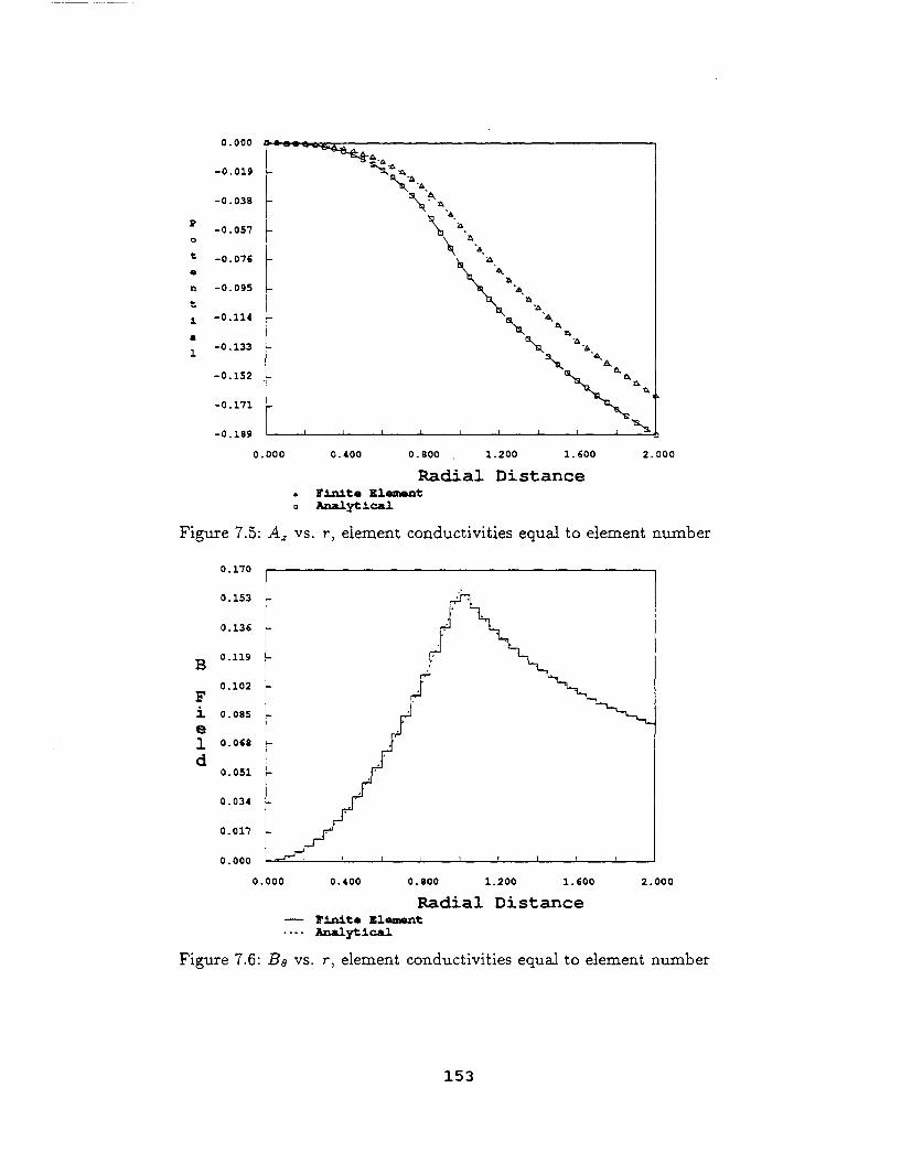
0.000
-0.019
-0.038
-0.057
-0.076
-0. 095
-0.114
-0,133
-0,152
-0.171
-0.189
0.000
N A
&,,_
0.400 0. 800 1.200 1.600
Radial DistanceFinite Elem_nt
Analytlcal
2.000
Figure 7.5: As vs. r, element conductivities equal to element number
B
Fie
1d
0.170
0.153
0.136
0.119
0.102
0. 085
0.068
0.051
0.034
0.017
0.000 ! I : I I I t
0.000 0. 400 0,800 1.200 I. 600
Radial Distance-- Finite Element
.... Analytical
2.000
Figure 7.6: Be vs. r, element conductivities equal to element number
153

7.4 SUMMARY.
The results obtained in the previous two problems show that it is
possible to extend the four-potential formulation to the case where the cur-
rent density distribution is unknown. This is important since this means
that it is now possible to solve problems where material and geometric non-
linearities preclude a Hnear current distribution. It also means that whereas
before a -1-1_owledge of how the current was distributed within a conductor
was necessary, with this extension of the four-potential variational principle,
all that is needed is the total current I through the conductor, its material
properties # and w, and the conductor geometry.
Having shown the validity of this extension of four-potential theory
to the prediction of electromagnetic quantities, one is now prepared to con-
struct a nonlinear conductor, the superconductor. This is the topic of the
next chapter.
154

THE SUPERCONDUCTING FINITE ELEMENT
In this chapter, the four-potential formulations of the Ginzburg-
Landau and London type superconductors are discussed. Both elements
use for the example problem the geometry of the one-dimensional infinite
conductor shown in Figure 2.1. Because the London type superconductor is
only an approximation to the more exact Ginzburg-Landau equations, only
the computational results for the Ginzburg-Laundau superconductor are pre-
sented here. _Ve restrict our consideration to the time-independent (static)
CaSe. -,
For both superconductors, the total current I is known, j is unknown,
and the static charge density p is zero. Because the four-potentia/method has
shown in the past three chapters that it can easily model the conductor/free
space boundary discontinuity for .Be, only the region within the conductor
is modeled. The stiffness and tangent stiffness matrices for the Ginzburg-
Landau superconductor contain the independent variables I¢[ and A and
therefore represent a set of non-linear equations. A short discussion of non-
linear solution techniques is included in this chapter as well as a discussion
on how [_/,[ and A are scaled to reduce the ill-conditioning of the system of
nonlinear superconducting finite element equations.
No analytical solution is available for the chosen problem. However,
numerical results can be examined to determine if they are physically re-
alizable. As a second check on the accuracy of the results, the B field as
155

determined by the finite element approximation using A can be compared
to the B field determined by j of the finite element formulation and Equa-
tion (7.1.5). Because no analytical solution is available, the first topic to be
discussed is the construction of the one-dimensional axisymmetric supercon-
ducting finite element.
¥
8.1 FINITE ELEMENT DISCRETIZATION.
As'mentioned in the introduction to this chapter, the discretization
of the Ginzburg-Landau equations results in a set of nonlinear equations. To
solve these equations, expressions for the residual r, the internal force vector
f, the external force vector p and the tangent stiffness matrix K are needed.
For this problem, f and r are determined by taking the first variation of the
governing functional, p by boundary integrals, and K by taking the second
variation of the governing functional. The relationship between r, f and p is
r = f- p (s.1.1)
In this section, r, f and K are determined and in the discussion of the
boundary terms, p is determined.
8.1.1 CDNSTRUCTING EM FINITE ELEMENTS.
For the finite element discretization of a one-dimenslonal supercon-
ductor, the two-node "line" element is again su_cient. Individual elements
are denoted by the superscript (e). As mentioned in Section 3.2.1, _ may be
replaced by _o with little loss of accuracy and this substitution is performed
for the superconducting finite elements derived here. The material parame-
ters a and _ are dependent upon T. Also mentioned in Section 4.1 is that
156

for the steady state heat conduction problem, Ir is a constant throughout a
superconductor. Consequently, the material parameters a, _ and #o are the
same for every element and the superscript (e) is omitted for these quanti-
ties. The element end nodes are denoted by the subscripts i and j. A: and
I¢1 are interpolated over each element as
A== A(<)= NA!') 1¢1= [_(_)1- Nl¢l(_) (8.1.2)
where the symbols A (e) and I_(e)[ have been introduced to simplify notation
later. The row vector N contains the isoparametric shape functions for the
interpolation of A: and I_#1. The elements of N are only functions of the
spatial coordinate r. A (e) and I_1 (e) contain the nodal values of A_ and ]¢1
respectively, and are time-independent. Substitution of these finite element
assumptions into the previously derived variational functional of Equation
(3.2.13) gives
aC')- .,v<<>fdV('){-<_t,¢I(')TNTNi,¢I(')+ _a (I,/.,I(<)TNTNI,/.,i(°))_
h2 T+ _m.I¢I(,)TON ON 1A(,)TONTONA(, )Or OrI@1(')+2vo : a,- Or
.2 -- T
+ _m.I¢I(')TNTNI¢I(')A(/) NTNA (_)}
(8.1.3)
Taking the first variation of AF_ e) gives a set of equations, which collectively
represent the internal force vector f for each finite element. The portion of
f(_) obtained by varying I¢l (_) is
Iv.,i= f dV(_) {-2<_NTNI¢I (<) +f(<) 2_['IS(e) 12NTNI¢i(")JV(_)
(8.1.4)
h 20NTON i.,/.,l(,)+ -_NTNi¢I(_)A (_)2+m* OF OF
157

The portion of the internal force vector associated with A (e) is
r { }f(¢)A, = dV(¢) 1 ON TONA_) + q I_(_)[2NTNA(_ ) (8.1.5)J v(_) #o (Or ar m*
The total internal force for each element is now
f(_) = { f(_)'_' } (8.1.6)f(e)A,
This expression applies to a Ginzburg-Landau superconductor. For a London
type superconductor [¢[2 is constant and equal to [¢_[2. Consequently, the
only nonzero portion of f(_) is f(_)A,.
Taking the derivative of f(e) with respect to the independent vari-
ables produces the tangent stiffness matrix K (e) for each element. The ex-
pression for a Ginzburg-Landau superconductor is
where
K(') = [[K(e)A'A:Id(e)TK(e)A'lt°l]L-_ A, hPl K(e)l_0[l_01
Jr(,) I_o Or O_ +-_ -EIffE(e)]2NTN
K(e)t,pll_ [ =
(8.1.7)
(8.1.8)
(8.1.9)
{( + 7i2 cONTON}m* ) m*& OrJV(_)
(8.1.10)
For the London superconductor K (*) is reduces to K(*)A, A,.
Examination of K(e)l¢ll,i and K(e)A:A: shows that an internal in-
consistency can appear because both of the independent variables, i¢1 and
158

Az, and their derivatives use the same shape functions. This inconsistency
can sometimes cause a "locking" problem. For the one-dimensional cases
considered here, this does not occur and is discussed further in Section 8.2.4.
For mechanical elements u (_) is the displacement field in the ele-
ment. In non-linear finite elements, v (_) are the visible degrees of freedom.
The nodal degrees of freedom v (e) cannot be solved for directly because the
internal forces are nonlinear functions of v (e), which in turn is a function of
the "loading parameter" (. The general technique to handle such nonlinear
problems is to convert the assembled residual force equations (8.1.0) to in-
cremental form by differentiating them with respect to a loading parameter
Of Of 0v 0p
8¢ - 0v a¢ - 0¢ or Kw = q (8.1.11)
where w is the set of incremental rates and q is the loading vector, w
and q represent the rate of change of v and p with respect to a loading
parameter C. The response v(_) is obtained by numerically integrating the
above equation in conjunction with Newton-Raphson iteration procedures
as described later in this chapter. The purpose of introducing these new
quantities here is that they are necessary for the topic of the next section,
the application of boundary conditions. In keeping with the new notation,
for a Ginzburg-Landau superconductor, v (e) and w (¢) are
{ oat?) }w (_) =
For a London superconductor, v (_) and w (_) are
OAtw(.,-
(8.1.12)
(8.1.13)
159

8.1.2 APPLYING BOUNDARY CONDITIONS.
The boundary conditions for Az are addressed first. As discussed
in the latter half of Section 7.2.2, the discrete boundary terms for the CU-
PLEID finite element are the same as those of a one-dimensional supercon-
ductor. The only non-zero values for PA, occur at the degrees of freedom
corresponding to the first and last nodal displacements of A,. They both
have a magnitude of H f and differ in the direction of their application. In
the past, f has been used to represent the total current load. It is now split
into two distinct parts to give
f = f_ + ell (8.1.14)
where fo represents the initial current and IL the loading current. When
the loading parameter _ is zero, the only load upon the system results from
the initial current load. When _ equals one, by convention the system is
regarded as being fully loaded. Using the new notation, the forcing vector
PAz is
/:}0PA, =(Io +(IL)H " (8.1.15)
where 1 and -1 correspond to the first and last degrees of freedom for A,
respectively, and the vertical dots represent a continuation of zeros over the
remaining degrees of freedom for Az. The expression for qA, is
0
OPAz = -ILH " (8.1.16)
qA" = (9"-_ 0
1
160

The above expressionsfor qA, and PA, are valid for any one-dimensional
conductor where the first degreeof freedom of A: is constrained to zero.
As discussed in Section 3.2.1,_'Ig_lon the boundaries is equal to
zero. Consequently, the boundary terms dependent upon l_I of (3.2.14)are
zero and make no contribution to p. The expressions for Plel and qleP are
therefore
PI,P] - 0 qle[ = 0 (8.1.17)
and the total external force and loading vectors are
p={PA,} q={qA_} (8.I.18)PIll ql*l
for a Ginzburg-Landau superconductor. To ensure that there are no su-
perconducting charge carriersin the free space surrounding the Ginzburg-
Landau superconductor, 1_] is constrMned to zero at r equal to re. For a
London superconductor, p and q reduce to PA, and qA_ respectively.
8.2 NUMERICAL EXPERIMENTS.
The finite element formulation for a Ginzburg-Landau superconduc-
tor has been applied to the solution of a one-dimensional axisymmetric infi-
nite wire. Each element contains two end nodes and a common global node
that is located at the truncation radius rt. These nodes are defined by their
-(') and _(e) The glodal node carries an "empty" degree ofradial positions r i rj..
freedom and is used only to provide the same number of degrees of freedom as
contained in the CUPLE1D finite element. Similarly, each end node contains
three degrees of freedom. The first and third degree of freedoms carry the
nodal values for I_b[ and Az respectively. The second degree of freedom is also
161

"empty". This choice provides for easier downstream coupling of the super
and normal conducting finite elements by reducing computational effort.
The computational effort is reduced because nodal connectivity and
freedom tables used to generate the diagonal location pointer array for the
skyline symmetric stored system of equations are only generated once. The
"empty" degree of freedom on each end node also allows for the easy addition
of the variable =_ if the gauge choice used is not the London gauge. With the
"empty" degrees of freedom, each element carries seven degrees of freedom
like the CUPLE1D finite element. The actual number of degrees of freedom
used per element is 2 x 2 = 4 degrees of freedom.
For the calculation of K, p, q and f the permeability # is set to #o,
as discussed in the introduction to Chapter IV. The values for a,/3 and I_ol 2
for each element are determined by using the formulas presented in Section
4.4. The tangent stiffness matrix and internal force vector are calculated by
numerical quadrature using a two point Gauss formula.
8.2.1 APPLYING BOUNDARY CONDITIONS.
The finite element mesh is terminated at rt, as in the linear conduc-
tor. To ensure that no superconducting flux can cross the conductor's outer
edge into free space, the degrees of freedom corresponding to ]¢1 between rc
and r, are set to zero. At r = re, l¢l is also set to zero. By doing this, the
boundary terms of (3.2.14) vanish. At r = 0, A, is set to zero as required
by the London gauge choice. Any "empty" degrees of freedom are also con-
strained to zero to prevent rank deficiencies of the assembled master stiffness
matrix.
162

8.2.2 ASSEMBLY AND SOLUTION.
The tangent stiffness and internal force vector are assembled follow-
ing standard finite element techniques. The tangent stiffness K is stored
using a symmetric skyline storage scheme, and then modified for boundary
conditions. The external force and loading vectors are inititalized to zero
and the two non-zero values for each are injected at the appropriate degrees
of freedom.
Solution Technique.
For linear finite elements, the displacements v can be solved for di-
rectly by inverting the stiffness matrix K u and multiplying it by the external
force vector p, i.e.,
= p (8.2.1)
The standard technique shown above to solve for v does not work for the
Ginzburg-Landau superconducting finite element because K u is a function
of [¢1 and A:. To begin our discussion of nonlinear solution techniques, the
residual equations are rewritten as
f-p = r = 0 (S.2.2)
where f and r represent the internal force and residual vectors respectively.
It can be seen that when the residual vector is zero, the solution vector v lies
upon an equilibrium curve or path called the response. The central idea of
non-linear solution techniques is to find a solution that lies upon a physically
correct equilibrium path and to then advance the solution along it. For
the cases examined in this work, the position along the equilibrium path is
determined by the loading parameter, also known as the control parameter, _'.
163

The displacements v are also called the state variables because they represent
the state of the system along an equilibrium path. For the cases presented
here, an initial solution that lies upon the physically correct equilibrium path
is not always known in advance. For these cases, we are required to guess
a "neighboring" state from which to start an iterative process that takes us
to the path. The initial solution, or "guess", is named the reference state of
the system.
For the Ginzburg-Landau superconducting finite element (STEP 1D),
it was found that the best choice for the reference state is that where Az is set
to 0 and all unconstrained values of I_l are set to I¢ool. The value for I¢0ol
is determined from the formula presented in Section 6.4. This state closely
approximates a Ginzburg-Landau superconductor with the total current I
and external B fields equal to zero, the difference for our choice occuring
primarily in the boundary layer. The true state can be closely approximated
by a step function for I¢1 over the interior of the conductor with a magnitude
of ]¢o¢]. However, the chosen reference state is close enough to the true state
that the same techniques used to advance the solution can also be used to
bring this reference state onto the desired equilibrium path.
To find how the solution vector v changes as the solution advances
along an equilibrium path, the partial of r with respect to the loading pa-
rameter ¢ is taken to give
ar af Op
Of Or Op
ov o¢ o(Ov
=K_--q
=Kw-q=O
(8.2.3)
164

The last equation shown above is known as the incremental rate equation.
K defines the tangent to the equilibrium path and is known as the tangent
stiffness matrix; w represents the rate of change of the solution vector along
the equilibrium path and is named the incremental velocity vector; and q is
the loading vector that represents the rate of change of the system's external
forces as the external loads of the system are varied.
To advance the solution along an equilibrium path, the values of the
solution vector at the current known state are used to determine the tangent
stiffness matrix. The loading vector is also determined and the following
system of equations is solved to determine the incremental rates.
w = K-lq (8.2.4)
Numerical problems arise, however, if the current position of the solution
on the equilibrium path is a stationary (critical) point. At these points, K
is singular. For the STEPID finite element, this occurs when AFg is zero.
There is no difference between the Helmholtz free energies for the supercon-
ducting and normal states of a conductor at this point. This point represents
a crossing of the equilibrium paths for the Helmholtz free energy functionals
of the normal and superconducting states and is called a bifurcation point.
If this point is reached or exceeded, because the free energies are equal, the
LETID finite element is used. The LET1D formulation is not singular at
this point because it does not contain the quantum parameter I_b]; conse-
quently it does not model the true state of the system at this point. The
true state is a mixture of normal and superconducting phases that lies be-
yond the modeling ability of one-dimensional finite elements as it is in fact
a multidimensional problem.
165

Assuming that a current value of v on the equilibrium path is "known,
as a first step to obtaining another solution, an increment along the tangent
to the equilibrium path is taken. That is, the solution is moved Av in the
v direction and A( in the ( direction of the hyperspace defined by v and (.
The step is named the predictor step. New values for v and ( axe computed
at the point that lies at the end of the predictor step. A corrector procedure,
called the correc_or step, is then invoked to iterate the solution back onto
the equilibrium path. The distances traversed in the v and ( directions for
each iteration are designated as d k and 77k respectively, where superscript
k designates the iteration number. The equilibrium path is reached when
r - 0. To ensure at each step n that the solution does not travel too far
from the equilibrium path, a distance l,_ is specified. The distance In is
also used to ensure that the distance along the equilibrium path traversed
is not too large. This distance is limited so that the solution procedure
does not accidentally step over a stationary point or move too far from the
equilibrium path. Detecting stationary points becomes important when they
are branching or bifurcation points because it is desired that the solution
procedure follow the equilibrium path that matches the true physics of the
system. If the solution procedure steps over one of these points, it may follow
a non-physical equilibrium path.
The addition of the length constraint adds an extra equation to the
original system of equations:
IzXs,_ ] - In = c = 0 (8.2.5)
where [As,l is an approximation to the distance s travelled on the equilib-
rium path. For the finite elements of this work, the initial values for v and
166

are computed using a Forward Euler scheme. The corrector step uses the
Conventional Newton-Raphson (CNR) method to iterateto a solution under
the arclength constraint (8.2.5). The formulas used for the forward Euler
integrationand the arclength constraint are reproduced below. Subscripts n
represent the step number and superscriptsk represent the iterationnumber.
Arclength Constraint
: .:nv.+ _¢-I-I.= 0la_.l-z.= T_
f. = q: + wrw.
0._.cc= aT _ Wn 0C 1@, so _- _- 7-:
(8.2.6)
Foward Euler Method with Arclength Constraint
A_, -- l,/f, sign (qTw,_)
(8.2.7)
To implement the Conventional Newton-Raphson technique, the
original equations for r must be augmented by the constraint equation c
and solved. This gives the linear system
(8.2.8)
Because this augmented system is not symmetric, the two linear symmetric
systems below are solved for instead
Kdr = -r Kdq = q (8.2.9)
167

to get
which finally gives
c + aTdr
r1 -- g + aTdq d = d,- + r/dq (8.2.10)
_k--k 1 _.. k _.k+l k,, v.+d .,. = _. +77 (8.2.11)
Iterations are performed until the 2-norm of r is less than a specified toler-
ance r. For cases where the 2-norm will not go below r, a limit is set on
the maximum number of iterations by another input parameter. Because the
Newton-Raphson technique can also diverge instead of converge upon a solu-
tion, limits on the maximum value for the 2-norm of v are also specified. To
stop the solution process, another input parameter limits the maximum value
of (. When this value for _ is surpassed, the solution process is terminated.
The solution procedure may be summarized as follows:
(1) Initialize v and ( to the reference state.
(2) Solve for w.
(3) Update v and ( using the Forward Euler integration scheme
(4) Evaluate r and c at step n + 1 by using v,+l and _,,+1-
(5) Solve (8.2.9) for dr and dq.
(6) Using (8.2.10) with the values for dr and dq, solve for 77and d.
(7) Update v and _ using(8.2.11).
(8) Find the 2-norm of v
(9) If the maximum value for the 2-norm of v or _ is exceeded, terminate
the solution procedure.
(10) Find the 2-norm of r and c.
168

(11) If the 2-norm of (10) is less than or equal to r, restart the solution
procedure over at step (2) until the desired value for _ is reached or
exceeded. If the 2-norm of (10) is greater than _-, go back to step (5)
and repeat the solution procedure until the 2-norm is less than or equal
to v or the maximum number of iterations is surpassed.
8.2.3 SCALING TECHNIQUES.
The solution procedure of the previous section is particularly sensi-
tive to heterogeneous physical dimensions in the solution vector v. In ad-
dition, off-diagonal terms of K may be either considerably larger or smaller
than the diagonal terms, giving K a high condition number. This means
that a small change in one degree of freedom may produce a large, non-
physical displacement at another degree of freedom. The STEPID finite
element solves the above problems by implementing several different scaling
techniques. The first technique gives the elements of v the same physical
dimensions. The second scaling makes off-diagonal terms of the same order
of magnitude as the diagonal terms. The third scaling is used to further
improve the condition number of K. Finally, the fourth scaling adjusts the
dimensions of v and _" in the solution hyperspace to improve convergence
rates and accuracy.
To perform the first, third and fourth scalings, the solution vector v
is scaled by a diagonal matrix Sn
_', = Shy (8.2.12)
where subscript n indicates either the first, third or fourth scaling and the
superposed tilde denotes a scaled quantity. If the stiffness-force equation is
169

premultiplied by S_ 1 and the scaled form of v is substituted, the results are
S_'IKUs[I-_ = S_lp
I_U÷ =(s.2._3)
where t( u and _ are the scaled versions of K u and p. The scaled versions of
other relevant quantities can be derived in a similar manner and are presented
below.
= S_ lr t' = S_ if ft = S_'lq
_r = S_'w _v = S_lAv I_ = S_IKS_ 1
la_l = _s_A_ + a< = l_ _ + A<l//
/= v/1+w_s_ = ,/1+._
First Scaling.
(8.2.14)
The first scaling is performed element by element at an element level,
and is used to scale I¢1 and Az to have the same dimensions. Let L, M,
T and Q represent units of distance, mass, time and charge respectively.
It can be seen that Az has units of ML/TQ and I_#t has units of L -3/2.
Numerical experiments showed that letting the units of v be L -1/2 improved
the stability of the solution process. For this scaling, S1 for each element is
expressed as
s;;) o o o1 0 0
s_;_ o
symm.
0 0 O"
0 0 0
0 0 0
0 0 0
i 0 0
s_;) o1.
(8.2.15)
170

fq,___2 q*
where ones have been placed at the degrees of freedom corresponding to the
"empty" degrees of freedom. This allows for the inversion of S_ e). Both
scaling factors are constants over the domain of the superconductor and do
not affect the assembled scaled master stiffness equations if this scaling is
performed at the elemental level.
Second Scaling.
The second scaling is performed to make off diagonal elements of K
of the same order of magnitude as the diagonal elements. It also serves the
dual purpose of bringing steps in the v-( hyperspace into a more reasonable
range. The second scaling is essentially a conversion of units from one system
to another. After performing the first scaling, the units of v are L -1 where
L is measured in meters, the appropriate unit of length for the rationalized
MKS system of measurement. However, most of the material parameters
for a superconductor are of the order of about 10 -s meters. To make the
order of magnitude of the off diagonal terms approximately the same as the
diagonal terms, it was observed that on an element level this could be done
by changing the units of length to micrometers (10 -s meters). To perform
_(e)-(_) and rj , are multiplied by l0 s.this conversion, all of the nodal positions, r i
The permeability of free space has units of M L/Q 2 and is also multiplied by
l0 s, whereas/i has units of ML_/T and is multiplied by 1012. The effective
penetration depth Ae/l has units of L and is also multiplied by l0 s. These
are the only quantities that are changed to perform the units conversion. The
remaining material parameters a,/9 and I_bool2 are calculated using the new
values for #o and Ae/f while the scaled value of/i is used for calculating $1
171

and K (_), B has units of M/TQ and is not affected by this unit conversion,
so scaled quantities can be used "as is" for field recovery.
Third Scaling.
The third scaling is performed on the assembled tangent stiffness
matrix K. It is a simple diagonal scaling where nonzero elements of the
diagonal matrix $3 are equal to the square root of the absolute value of the
corresponding diagonal element of K, i.e., Sii = _. For the "empty"
degrees of freedom, the diagonal elements of $3 are set to one to give full rank
to the matrix so that it can be inverted. This is a common scaling technique
that will reduce the condition number of a symmetric positive definite matrix.
Although the constrained stiffness matrix for the superconductivity problem
is negative definite, this technique works well here.
Fourth Scaling.
The fourth scaling is also performed on a global level. Again a diag-
onal matrix $4 is used, but this time all of the elements are the same. The
purpose of this scaling is to make A_ approximately equal to l,. To meet this
requirement, f must be approximately one. It is ensured with this require-
ment that no matter what the value of the product wTw may be, the scaled
distance traversed along the equilibrium path will be approximately equal
to the desired input distance 1,,. The value for each element of $4 that gave
the best results for the STEP1D finite element numerical examples presented
here was 10 4 .
172

8.2.4 MESH GENERATION.
The superconductivity problem exhibits boundary layercharacteris-
ticsbecause most of the physics occur in a relativelynarrow region close to
the conductor/free space boundary. The finiteelement mesh must have a
finegrading in thisregion to model superconductivity accurately. Eighteen
months of research and numerous numerical experiments have shown that
ifthe mesh grading there isinappropriate, the solution generated will suf-
fer accordingly. The problem most often encountered by poor mesh choices
was that of a high condition number for K. This generally causes the so-
lution method to failbecause the 2-norm of the residual vector r and the
arclength constraint c cannot be brought below a reasonable value for the
input tolerance T. The solution "dances" around the v - [ hyperspace until
the maximum number of correctoriterationsisreached or the 2-norm of v is
exceeded. In a few rare cases,with a poor mesh choice,the solution actually
did converge. These solutionswere rarelyof any value because the condition
number was estimated to be in the to range of 106 to 1016! Another diffi-
culty encountered with a poor mesh choice is that I%$1and .4= willoscillate
around theirequilibrium values. To solve these problems, it isnecessary to
reexamine the theory of superconductivity.
In the previous discussionof superconductivity,the effectiveLondon
penetration depth )_effwas introduced. The London penetration depth pro-
vides a measure ofhow far the B fieldpenetrates intoa superconductor from
the conductor/free space interface.This issignificantbecause Aeff provides
a minimum depth for the boundary layer that isbeing modeled. This isthe
173

range over which A, should decay to approximately zero. It is also neces-
sary to know the range in which the other variable, ]_1, decays from its bulk
layer value of 1_oo] to zero. To accomplish this goal, the Ginzburg-Landau
equations must be examined once again. The following is an abstraction of
material presented in Reference[ 21], pp. 111-114, and is used to determine
the range of decay of 1_31.
The variation of/kFg for a one-dimensional superconductor in Carte-
sian coordinate space will produce the Euler equation
_2 a2I#_I+ el't/,, I - #I¢I 3 = 0 (8.2.16)
2m* ax 2
where x is the one-dimensional spatial coordinate and A has been set equal
to zero because we are primarily interested in the behavior of J¢l- If the
normahzed wave function I¢lN which equals 1¢1/1¢o_1 is introduced, and
some algebra is performed, Equation (8.2.16) becomes
_2 a21¢lN -l_'l_v = o2,.,.,x,__ + I¢IN (8.2.17)
Linearizing this equation by setting I_']N equal to 1 + b(x), where b(x) <<I.I,
gives the first order expansion of this equation as being
_2 O2b(z)2rn*a Oz. 2 = -(1 + b(x)) + (1 + 3b(x))
=-7- (), ~(8.2,18)
The first term of the equation shows that the decay of ]¢]N is determined
by _//h2/2rn*o. This length is referred to as the Ginzburg-Landau coherence
length _(T). Appropriate substitutions from Chapter IV will give
!
_(T) - v_q*l I - (T/To) 2 (8.2.19)
174

To avoid confusion with the isoparametric coordinate _, this length shall
always be referred to as _(2-). The dimensionless Ginzburg-Landau param-
eter ,:(7") is also introduced, which is the ratio of the two lengths 4(T) and
A,::(2-).
where _(iF) shall be used for this ratio to distinguish it from the Lagrange
multiplier vector _. A superconductor with t¢(2-) < 1/v_ is called a type I
superconductor, while a superconductor with t¢(2-) > 1/v_2 is called a type
II superconductor. Figure 8.1 shows the difference between _(T) and AeH
for type I and II superconductors.
For the particular case of high purity aluminum, _(0) _ .1. This
makes it a type I superconductor and shows that the decay depth for I_1 is
approximately ten times the decay depth of A:, where Ae]] is the approx-
imate decay depth for Az. Consequently, the boundary layer region to be
modeled must have a depth of at least 10 x Aef] to capture I¢I, furthermore
_(T) determines the size of the boundary layer mesh. For a type II super-
conductor Ae]](2-) > _(2-) and the size of the boundary mesh is determined
by Aef](T). Numerical experiments confirm that for aluminum the mesh
choice of 10 × Ae]] reduces the condition number of the system. Numerical
experiments also show that the mesh generated must be a function of 2"
because Ae]] and _(T) are both functions of iF. The results obtained with
the above mesh show realistic values for I¢[, but both [_[ and Az exhibit
oscillatory behavior. Expanding the boundary layer depth to 200 x Aeff
caused the oscillations in I_l to disappear. All elements generated in the
175

B
._....Conductor
Boundary
Type I Superconductor
B
_.....Conductor
Boundary
_ k
Type II Superconductor
Figure 8.1: Differences between B, _, _(T) and _eff for type I and II super-conductors.
176

boundary layer were equal length elements, where the element length was
equal to the depth of the boundary layer divided by the number of boundary
layer elements Nbo,nd. The elements used to model the bulk layer were also
"regular", their length being equal to (re - 200 x A,f/(T))/Nb_k, with Nb_tk
representing the number of bulk layer elements.
The oscillations are triggered by three different error sources. The
first one comes from the approximation that is made for (8.2.18). The
Ginzburg-Landau equations are linearized there to get an idea of the pen-
etration depth of the magnetic field. The coherence length is only a rough
approximation to the true penetration depth and not an exact one because
only the lineaxized system of equations has been solved and not the exact
system. The second source of error arises because the finite element model
is not exact. It merely tries to approximate the continuous case by discretiz-
ing the region of interest. The third source of error is that finite precision
mathematics are used when a solution to the discretized superconductor is
attempted. The solution procedure and the scaling procedures used all in-
troduce numerical error into the computed solution because of the machine's
inability to resolve numbers beyond 16 significant numbers. The expansion
of the boundary layer helps to push the oscillations induced by the numerical
error of the solution and scaling techniques below machine limits and more
importantly, accurately captures the physics of the problem.
After the oscillations in I¢[ are removed, Az may still exhibit oscilla-
tions close to the conductor/free space boundary. It was thought that they
were induced by the mesh being too coarse for that region. Numerical exper-
iments showed that this was indeed the case. There are three methods that
can be used to resolve this problem. The first method consists of generating
177

another boundary layer of regular elements near the conductor/free space
boundary. The second method involves changing the length of each element
so that the mesh is more finely graded at the conductor/free space boundary
than at the interior edge of the boundary layer. The third method is to
simply insert more elements into the boundary layer. All three methods add
extra node points at the conductor/free space boundary and serve to make
the finite element approximation more accurate. The third method was used
for the examples here to expedite the research. This is the least compu-
tationally efficient of the three, but time constraints limited the author to
using this choice.
It is mentioned earlier in Section 8.1.1 that the use of the same shape
functions for the calculation of I¢l and A: and their derivatives can lead to
internal inconsistencies that can cause a "locking" problem. As the length of
the element l(_) goes to zero, the polynomial shape function approximation
of the independent variable tries to match the approximation of its first
derivative, which is a constant, when 'locking" is present. This leads to the
oscillatory behavior described above. But as more and more nodal points are
added, i. _., more finite elements are added, oscillations of the independent
variable will still persist if "locking" is present. These oscillations disappear
for the STEP1D finite element as the mesh is refined and show that "locking"
is not present for the one-dimensional cases studied here.
To summarize, the depth of the boundary layer mesh is determined
by the larger of A,I/ and _(T). This is the starting point for determining
the boundary layer depth. Numerical experiments are then used to expand
the boundary layer until oscillations of I%bl disappear. Finally, additional
178

elements are inserted into the boundary layer until oscillationsof A.. also
vanish.
8.2.5 FIELD RECOVERY.
The primary quantity of interest is again B. For this problem, there
is no analytical solution, but the results can be checked to determine if
they are physically correct. There are also two methods by which B can be
determined from the finite element solution. Comparison of the results of
these two methods determines if an internally consistent solution has been
reached.
The first method of determining the Be field is the finite element
approximation of Equation(5.3.2). The second method uses Equation(3.2.16)
inserted into Equatition (7.1.5). The one dimensional form of this equation
that gives the value for Be at the outer node of each element e is
"J ,_=_ I") 12,,4('_) rdr (8.2.21)
where the superscript letter in parentheses represents an element number.
The integration over each element is performed by numerical quadrature
using a two point Gauss rule.
8.2.6 TEST PROBLEM.
The test material used for this example was high purity aluminum.
The material constants a and fl for each element were evaluated at T equal to
zero degrees Kelvin using the formulas of Section 4.4. The permeability # of
each element was set to #o as discussed earlier in this chapter. The reference
state of v was set as described in Section 8.2.2. The mesh was discretized
179

as desribed in Section 8.2.4 with a regular mesh of Nb,tk elements in the
region 0 _> r > re - 200Aeff. Another regular mesh of Nbo,,nd elements was
generated in the region rc - 200Ae// >_ r > re. Nb_tk and 2Vboun d denote
the number of elements in the bulk and boundary layers respectively. Nb,,k
and Nbo,,nd were 2 and 98 for this problem respectively. Because the free-
space magnetic field element has been validated previously, all elements were
within the conductor. The conductor radius rc was 1.15 x 10 -4. The value
of Io was 5.0 amperes and the value of IL was 0.0 amperes for the results
presented here. The choice of these values ensures that an actual specified
current loading for results presentation was attained. The element has been
tested many times by loading from zero to full load and has worked extremely
well. The only problem that was experienced was when the current loading
appoached a magnitude that was large enough to move the solution close to
the stationary point. In this region, Av and A_ became increasingly smaller.
To rectify this problem, the coding was modified to ensure that the step size
at step n + 1 does not fall below an arbitrary value. If the step size became
too small, .9 × I, x IL was added to Io, the reference state was reset, and
the solution proccedure was restarted at step n. The only disadvantage to
this scheme was determining the correct value of I at each step for output
purposes. This problem was easily circumvented by outputting the value for
Io when it changed, and the step where the change took place.
The main disadvantage with using the incremental solution methods
for results presentation was that the solution process did not always stop at
the desired full load value, but usually exceed it by some fraction of the step
size ln. This is a consequence of the solution procedure used, and is inherent
180

in arclength schemes. By setting IL equal to zero and Io equal to I, this
problem was bypassed here.
For the results presented below, the solution procedure required 9
iterations to converge, with the solution tolerance _- being 4 x 10 -17. The
2-norm for r did not include the value for the constrained degree of freedom
of ItbI. The value of r there ranged between 10 -3 to 10 -7 depending on how
close the finiteelements came to modeling a zero slope for I_Iat the conduc-
tor/freespace boundary. To more accurately match thisslope requirement,
allthat was needed was a more refined mesh for this area. However the
resultsobtained were judged accurate enough for our purposes. Finally,the
estimated condition number of the system was 228.
Figures 8.2 and 8.3 show the resultsobtained for the normalized val-
ues of I_I2 plotted over the whole conductor and the boundary layer of the
conductor respectively.Ifa London type superconductor had been modeled,
an exact step function would have been expected. Because aluminum isan
extreme type I superconductor, I@I should exhibit behavior that is almost
"step"-like.Figure 8.2 illustratesthat the finiteelement does model phys-
icalbehavior by returning values that closelymatch a step function. The
boundary conditions are seen to match wellin Figure 8.3 in that the slope of
I@N 12iszero at the interiorboundary and isvery closeto zero at the exterior
boundary.
Results forAz are shown in Figures 8.4 and 8.5.Figure 8.4 shows the
behavior over the whole mesh and Figure 8.5 the behavior in the boundary
layer. The physical behavior of A= should approximately be the opposite
of I#]- Over the bulk of the conductor, Az should be zero, and where I@l
181

1.250
PS
i
NO
rma1i
Z
ed
1.125
1.000
0.875
0.750
0. 625
0.500
0.375
0.250
0.125
0.000 -----I
0.000
J £
2. 875 e-5 5.750 e-5 8.625 e-5 1.150 e-4 1.4375 e-4
Radial Distance
Figure 8.2: f¢t2/]¢o0[ 2 vs. r, values for complete mesh plotted.
1.250
P
si
N
orma1iZ
ed
1.125
1.000
0.875
0.750
0. 625
0.500
0.375
0.250
0.125
0.000
1.120 e-4
I I I
1.126 e-4
I
1.132 e-4 1.138 e-4 1.144 e-4 1.150 e-4
Radial Distance
Figure 8.3: [¢12/[¢o0[ = vs. r, values for boundary layer plotted.
182

Poten
tia
1
0.000
-2.97025 e-4
-5.94050 e-4
-8.91075 e-4
-0.001 -
-0.001
-0.001
-0.002
-0. 002
i-0.002
-0.003 !
0. 000
I ' I i I i
2.875 e-5 5.750 e-5 8.625 e-5 1.150 e-4
Radial Distance
1.4375 e-4
PO
t
e
n
tia
1
Figure 8.4: Az vs. r, values for complete mesh plotted.
0.000
-2.97025 e-4
-5.94050 e-4
-8.91075 e-4
-0.001
-0.001
-0.001
-0.002
-0.002
-0.002
-0.003
1.120 e-4
I I I r I t F 1 I
1.126 e-4 1.132 e-4 1.138 e-4 1.144 e-4 1.150 e-4
Radial Distance
Figure 8.5: Az vs. r, values for boundary layer plotted.
183

decreases, the magnitude of Az should increase as kinetic momentum is ex-
changed for magnetic field momemtum. Figure 8.4 shows this expected phys-
ical behavior. Figure 8.5 shows this behavior in more detail, and illustrates
one difference in behavior between Az and I_]. The slope of Az is zero at the
interior edge of the boundary layer, but nonzero at the exterior edge. This is
expected because the boundary conditions for Az and I_] are different at the
exterior edge, the behavior of Az matching its expected physical behavior.
Figures 8.6 and 8.7 display the results for jz over the entire conductor
and the boundary layer respectively. The behavior of jz can best be described
by making an analogy to a similar problem in fluid mechanics. The medium
of the problem would be a large pool of water contained between two infinitely
long straight walls. For convenience, the walls are aligned so that one is on
our left side and the other on our right. To make the analogy correlate to the
results presentation, the left wall would be the center of the superconductor,
and the right wall would be the conductor/free space boundary. The bottom
of the pool would be shaped so that the density of water molecules matches
the density of the superconducting charge carriers. The walls and the bottom
of the pool would present no resistance to water flow. Assuming laminar flow,
a rapidly moving stream of water is injected into the pool along the right wall.
For the EM problem, j: is analogous to the velocity of the water molecules,
vw in the pool. Where the stream is injected, it is expected that a large,
rapid change in v_ would exist, which upon first examination would appear
to be a Dirac delta function.
This behavior is exactly matched by the velocities of the supercon-
ducting electron pairs of the finite element model, and is shown in Figure 8.6.
At the conductor/free space boundary, a Dirac delta-like "spike" appears for
184

0.019
0.017
0.015
0.013
0.011
0.009
0.007 _-
0. 005
0.004 i
0.002 I0.000
0.000
t r J i I I
2.875 e-5 5.750 e-5 8.625 e-5 1.150 e-4
Radial Distance
1.4375 e-4
C
u
E
E
n
Figure 8.6: jz vs. v, values for complete mesh plotted.
0.019
0.017
0.015
0.013
0.011
0.009
0.007
0. 005
0.004
0.002
0. 000
1.120 •-4
I I r I I I f
1.126 •-4 1.132 e-4 1.138 •-4 1.144 •-4 1.150 •-4
Radial Distance
Figure 8.7: j_- vs. r, values for boundary layer plotted.
185

j:, which is zero otherwise. A closer examination of the fluid velocities for
the imaginary example would reveal that v_, would rise rapidly on both sides
of the stream, but a more gradual rise in v,, would occur on the side of the
stream facing the left wall as momentum is exchanged with the other water
molecules there. Again j: mimics this behavior as shown in Figure 8.7 and
validates the ability of the STEP1D element to model the expected physics
of a superconductor.
This comparison of a fluid flow to a Ginzburg-Landau supercon-
ductor is a particularly enlightening one because, if this superconductivity
model is correct, it explains the source of the miniscule resistivity in super-
conductors. The resistivity is a result of a momentum exchange produced by
colhsions of Cooper pairs, the supeconductor's charge carriers, as required
by the residual equation (3.2.6). Because the collisions are relatively infre-
quent, a "spike" in the current density appears in the boundary layer, rather
than a _%mearing" of the current density to an approximate step function.
The position of the spike is determined by the density of charge carriers, the
current density vector choosing the point where the fewest collisions can take
place. The fact that the density of Cooper pairs is higher on the interior of
the boundary layer than the exterior explains why j, changes more slowly
towards the center of the conductor. The Cooper pairs in the current stream
j: are simply experiencing more collisions with stationary Cooper pairs be-
cause the density of pairs is higher towards the center of the conductor. Its
position also determines that there is an expulsion of the B field from the
interior of the conductor (the Meissner effect) because there is no current
there to generate a field in accordance with Maxwell's equations.
186

0.010
B
Fie
1d
0.009
0.008
0.007
0.006
0.005
0.004
0.003
0. 002
0.001
0.000 I I I T I I ! I
0.000 2.875 e-5 5.750 e-5 8.625 e-5 1.150 e-4 1.4375 e-4
Radial Distance
B computed using potential
B computed using current density
Figure 8.8: Be vs. r, values for complete mesh plotted.
0.010
B
Fi
e
1d
0.009 .
0.008
0.007
0.006
0.005
0.004
0.003
0.002
0.001
0.000
/
r _ i L I L I ,. I
1.120 e-4 1.126 e-4 1.132 e-4 1.138 e-4 1.144 e-4 1.150 e-4
Radial Distance
-- B oomputed uaing potential
.... B computed using current density
Figure 8.9: Be vs. r, values for boundary layer plotted.
187

Figures 8.8 and 8.9 show the Be field generated there. Figure 8.8
shows Be over the whole conductor and Figure 8.9 shows Be in the boundary
region. Because no analytical solution is available, the B field has been
plotted using the two different methods cited previously and finite element
values for I_bl and A=. As in Chapter VII, the Be field calculated using
Equation (5.3.2) is plotted as a step function. Both sets of values match
fairly well over most of the region, but show some divergence towards the
maximum and minimum values of Be. No reason exists to prefer one set of
values over the other, but using j(e) to recover Be has the advantage of being
able to directly compute Be at element nodes.
Expected physical behavior is matched by both curves. The value of
Be computed by using (8.2.'2_1) also matches the necessary analytical value,
derived from an integral form of Maxwell's equations, of #oI/27rrc. A com-
parison of these values with values obtained by using the London model of
superconductivity does not allow any statement to be made about the accu-
racy of the Ginzburg-Landau model because the former neglects the o_radient
of I_bl. The important point is that the Ginzburg-Landau model must achieve
a specific magnitude at re, and this is verified by Equation (5.3.2). For the
above reasons, the London vMues are not compared to the finite element
values obtained here.
8.3 FURTHER DISCUSSION OF RESULTS.
A word of caution isnecessary here with regard to the author's phys-
icalinterpretationof results.Because no analyticalsolution isavailablefor
188

comparison with the numerical results, these results and their physical in-
terpretation must he treated with some suspicion pending experimental ver-
ification. However, there is a good evidence to suggest that the results are
valid.
First, the numerical approach has been based upon the Ginzburg-
Landau theory of superconductivity. This theory, while not being thoroughly
validated experimentally for cases away from the critical temperature, has
been able to predict superconducting phenomena with a great deal of accu-
racy (R.ef. [21, pp.104-191]). This provides a great deal of credibilty to the
ability of the Ginzburg-Landau theory for the prediction of EM and quan-
tum phenomena within a superconductor. It is universally accepted as an
accurate model of the macroscopic quantum-mechanical and electomagnetic
properties of a superconductor near its critical temperature To.
Second, the results of this chapter and Chapter XI exhibit behavior
that is in qualitative agreement with the physics of superconductors. These
behaviors are the appearance of the Meissner effect and a current carried
at the surface of a superconductor. The Meissner effect is the almost total
expulsion of a magnetic field from the interior of a conductor, and this be-
havior is shown in Figures 8.8 and 11.12. The cause of this effect is that the
current is carried at the surface of the conductor (Ref. [31, p.335]). In order
to satisfy Maxwell's law _ × xy × B = j, no current can be carried within the
bulk of the conductor or a magnetic field will be present there. Again, the
STEP1D finite element shows this behavior in Figure 8.6.
Finally, there is some quantitative agreement between the STEP1D
finite element and a known physical value. The value of the Be field at the
189

conductor radius is known to be #oI/27rrc. As mentioned at the end of the
prewio.us section, the finite element model achieves this value at rc.
8.4 SUMMARY.
In this chapter, a broad range of topics necessary to the solution of
the superconductivity problem by the finite element method are discussed.
The topics include the four-potential formulation of superconductivity, ap-
propriate boundary conditions, nonlinear solution techniques, scaling tech-
niques, and appropriate mesh choices for finite element models. The most
important aspect of this research is the insight that is gained about super-
conductivity. For the Ginzburg-Landau model, it is possible to think of
the current that moves through a superconductor as a "stream" of charge
carriers called Cooper pairs that moves through a "sea" of static Cooper
pairs. This "sea" acts like an extremely low viscosity fluid, and the "stream"
moves through the region of the "sea" where the density of the Cooper pairs
is the smallest. This region represents the place where the least amount of
ener&,3r is expended by the collisions of mowing Cooper pairs with station-
ary Cooper pairs. Unlike the London approximation, or linearized forms of
the Ginzburg-Landau model, the physics of the system as described above
are Shown only by modeling the exact Ginzburg-Landau equations so that a
complete description of jz can be obtained. The STEPID model shows this
behavior well, and from the limited search of literature that the author has
performed, it is believed that this is the first model that shows the physics
in such good detail.
Now that reasonable models for the normal and superconducting
states of a conductor have been developed, the next step in the complete
190

modeling of a conductor is to add thermaJ ei_ects. This is the topic of dis-
cussion of the next chapter.
191

THE THERMAL PROBLEM
It is first necessary to model the temperature distribution within a
conductor l_efore the effects a temperature field has on the EM fields and the
quantum properties of a conductor can be determined. Appropriately, the
first topic of discussion in this chapter is the modeling of the temperature
field of the steady state heat conduction problem with convection cooling
boundary conditions. The one-dimensional case is the case of interest for
this work's examples and is the only case discussed. In Chapter IV it is
mentioned that there are no temperature gradients within a one-dimensional
steady state superconductor. Because no gradients are present, the temper-
ature distribution of a superconductor is known and the calculation of the
temperature distribution by finite element methods is not necessary. There-
fore, this chapter is concerned with the finite element modeling of a normal
conductor. The temperature distribution within a conductor is a function
of the current I and the thermal boundary conditions at re. In the current
chapter, it is assumed that the current I is steady and does not change.
Cases where the current load I changes are discussed in the following chap-
ter. For this chapter, the discussion is about the physics of a conductor as
the thermal boundary loads are varied.
The discussion begins by first developing the finite element model
for the temperature distribution of a one-dimensional conductor, and then
determining the analytical solution of that problem. The analytical solution
192

to this problem is developed later because certain assumptions about the
finiteelement model have a directeffecton the analyticalsolution.
9.1 FINITE ELEMENT DISCRETIZATION.
9.1.1 CONSTRUCTING THE LINTID FINITE ELEMENT.
Using the two-node "line" finite element again provides the C ° conti-
nuity required by the variational functional of(4.1.7) for 7". Again individual
elements and elemental properties are identified by the superscript (e). The
two element end nodes are denoted by the subscripts i and j. The tempera-
ture 7" is interpolated over each element as
7" = N7- (e) (9.1.1)
where the row vector N contains isoparametric shape functions for the inter-
polation of 7". The elements of N are functions only of the spatialcoordinate
r. The column vector 9-(¢)contains the nodal values of :7",which are con-
stantswith respect to time. Substitution of these finiteelement assumptions
into the variationalfunctional of Equation (4.1.7)gives
= -T t _ -- --T J w(_)j(_)27"(")TNTJ V(') 2-- Or Or --
(9.1.2)
Variation of the above with respect to 7-(') will produce
(9.1.3)
193

Quantities k and w (')are functions of the spatialcoordinate r and no_ of the
independent variable T. This assumption is made because the variational
functional I'I_') does not give the correct residuals for the heat conduction
problem if the thermal conductivity and the electrical resistivity are allowed
to be functions Of 7". This approximation can be corrected by using the
nonlinear solution procedures of Chapter VIII. During the solution phase, k
and w (_) are held constant at their values for step n, and after the solution
vector v at step n + 1 is determined, k and _o(e) axe updated using the new
temperature distribution of step n + 1. If the step size l,_ is small, v does not
move too far from the true equilibrium path and the values of_.T (e) are close
enough to the exact values that any error is negligible. This assumption is the
reason for discussing the finite element model first instead of the analytical
solution. No analytical solution exists for the set of coupled EM-thermal
equations where k and w are functions of 7-. By making the approximation
that k and w axe functions of the spatial coordinate r, an analytical solution
can be developed.
The spatial approximations used are the ones discussed in previous
chapters, i.e., w is a step function or constant over an element, and k is
interpolated linearly across the element. In terms of our shape functions, k
may be written as
k = Nk (_) (9.1.4)
where k (_) contains the nodal values of the thermal conductivity. The values
for k (e) are obtained by using Equation(4.2.1). Equation(4.2.1) is a function
of T, and is evaluated at T/(_) and 7-/e) to obtain the respective components
of k (e), k} e) and k/). For the evaluation of k (_) and w (_), T/(e) and Tj (e)
194

are the two components of .T_.T(*) at step n. The elemental value for w(*) is
determined by the formula
where O_o is the residual resistivity, and wi(T) is the ideal resistivity. The
ideal resistivity is calculated as described in Section 4.3.
All but two of the boundary integrals of (9.1.3) can be ignored by
noticing that the heat flux Qr between interelement boundaries in the radial
direction must be C O continuous; this point is shown later by the analyt-
ical solution. The two remaining boundary integrals occur at r equal to
zero and re. At r equal to zero, itcan be seen that the boundary integral
there vanishes,and the only remaining boundary integraloccurs at re. The
remaining integral is a function of the boundary heat flux loading where
Qr((r) represents this load and _Ir is the thermal loading paramter.
Because non-linear solution techniques are used, expressions for K (_) ,
f(*), r (*), p(*) and q(*) must be determined. The Euler equations of (9.i.3)
give the following expressions for r (*), p(*) and f(*)
f( )=fdV( ){kONTONT( )}Y V(_) Or Or --
p(,)=[ dV(, ){w(,)j(/,2NT}+Snt, {27rrcQr(_Ir)}] {0} (9.1.6)d v(,) r, 1
r(,) = f(e) _ p(,)
where the Kronecker delta 5{j is defined as
= 0 i # j
=1 i=j
(9,1.7)
195

i rn = Nwire + 1, with Nwir_ again representing the number of elements in
the conductor. Taking the partials of r with respect to 7 "(e) and _T produces
the following expressions for K (e) and q(e).
Jr(,) [ -_r _ (9.1.8)
r OQ,( r) o
where j(¢) and w (e) have been assumed to be only functions of the nodal
position r and thereforevanish.
9.1.2 APPLYING BOUNDARY CONDITIONS.
In the previous section, expressions for p(e) and q(¢) are determined.
They contain the boundary heat flux term Qr(_T). The heat flux at rc for
the one-dimensional steady state convection cooling problem is expressed by
the Euler equation of (4.1.10)
Q,=h_o._(7"_-7-(r_)) (9.1.9)
Because the free stream temperature 7"_ is known, it is natural to choose
this variable as the load to be varied. To make T_ a variable load, it is
split into two parts where To is the initial loading temperature, and TL is the
variable loading temperature. The free stream temperature is now expressed
as
= % + (9.1.10)
The value of the temperature at r equal to re can also be expressed as
T(rc) = NjTj (m) = Tj(m); m = Nwi,e + 1 (9.1.11)Tc
196

where Nj is the second component of the shape function vector N, _(m)
is the nodal value of the temperature at re, and the superscript letter in
parentheses represents an element number and not an exponential. When the
new expressions for T_ and 3-(re) are substituted into (9.1.9), the expression
for Q,.(¢7) becomes
Qr(
and the expression for c_Q,-(¢7)/0_ v" is
OQ,.((7)
C3_7 -- hco._ TL a_ 7 = hco,_v 7"L--W ")/(_ _ (9.1.13)
where w_ m) is the nodal value of the incremental rate of change of 7" at rc.
By convention, any terms of a set of finite element equations that
include the incremental rates and the nodal displacements are usually moved
to the left hand side of the system of equations. Doing this, and making
substitutions for Qr(_ _') in the previously derived vectors p(e) and f(e) gives
f(,) [dV.(_){kaNTaNT(_)_ [0 O1]T(_)=Jr(.) 37 3;-,- j -
P(')-'-/J v(,:ldV('){w(')J_')2NT}+6"'{2?rr'h'°n'(T°+#mTL)}{ 01 }
(9.1.14)
Similarly, K (_) and q(_) are
-- JV(¢) Or Or + 6me {27rr¢} 1
q(e) - 6'ne {27rrchc°n"TL } { 0 }1
The addition of the boundary term Q_ makes this system of equations, when
assembled, determinate and no nodal values need to be constrained.
197
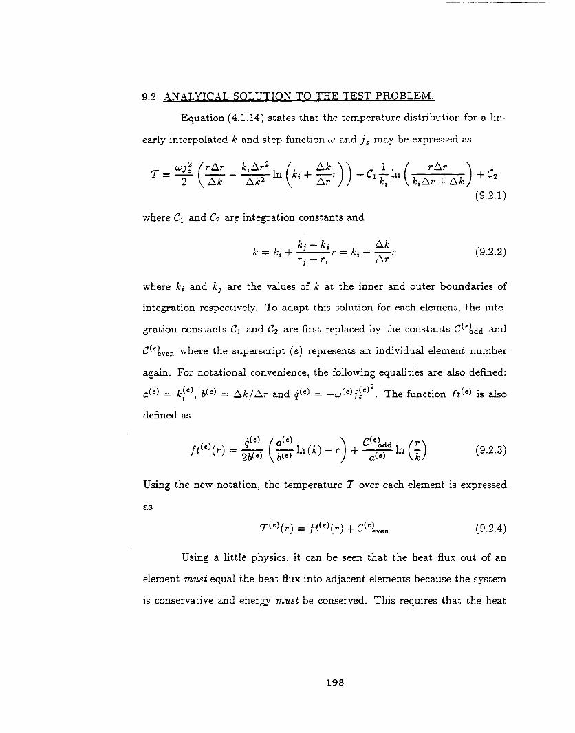
9.2 ANALYICAL SOLUTION TO THE TEST PROBLEM.
Equation (4.1.14) states that the temperature distribution for a lin-
early interpolated k and step function _ and jz may be expressed as
2 Ak Ak 2 _ ] +CI . in kiAr + Ak +C2
(9.2.1)
where C1 and C_ are integration constants and
kj - k_ Akk = ki + --r = ki + --r (9.2.2)
r I -- ri Ar
where ki and kj are the values of k at the inner and outer boundaries of
integration respectively. To adapt this solution for each element, the inte-
gration constants C1 and C_ are first replaced by the constants C(¢)odd and
C('),,e n where the superscript (e) represents an individual element number
again. For notational convenience, the following equalities are also defined:
a (') = k$ e), b(e) = Ak/Ar and q(') = _w(,)j(,)2. The function ft (') is also
defined as
ft(')(r) = 2-_ k b-_ in(k) - r + a(-----S-
Using the new notation, the temperature T over each element is expressed
(9.2.4)
as
T(')(r) = ft(e)(r) + C('),,e.
Using a little physics, it can be seen that the heat flux out of an
element must equal the heat flux into adjacent elements because the system
is conservative and energy must be conserved. This requires that the heat
198

fiux Qr be C ° continuous and gives the following seriesof equations that
relatethe heat flux transferredacross adjacent element boundaries
c%_a _('>_I_ C('-_oaa q(_-_>_/-_>(_-1) 2
rl ¢) 2 rj(9.2.5)
This equation can be rearranged to give
C(_)odd = q(_)r__)2 --_)(_--_)_"_ c(e-l)odd __ _(e rj2 2
(9.2.6)
by using the relation r (e-l) _(e) At r equal to zero, C(1)odd must also bej ---- z-i .
zero for the system of equations to remain bounded. This gives for C(e)dd
C(e)odd = 2' -- A-Jp=l r_ -- e > 1
= 0 ¢=1
(9.2.7)
The values for C (¢)even may be derived in a similar manner by ensuring that
7" is C ° continuous across element boundaries. The result is
,. even= - t (e)( (e) l -"<_) _ s ,,,, _ {st,(v;) S_.(rf)}p_e
(9.2.8)
where _ is the temperature at the surface of the conductor and equals the
nodal value Tj("0. Ts is determined by using the discretized version of Equa-
tion (4.1.21), which is
1 w(e)j_¢)_ rh_o.,,ro_ dr (9.2.9)e=l I ")
The preceding analytical solution is only valid for cases where b(0 is
nonzero. As k} _) approaches _!_) the first two terms of (9.2.3) diverge. For
199

cases where b(*) is zero, the methodology used to derive (9.2.1) in Chapter
IV can be used to determine that ft(*)(r) becomes
q(*) r 2 + C(e)odd 111(7") (9.').10)ft(e)(r) = 4
The methods of this section can then be used to show that the solutions for
Ts, C(*)dd, and C(e)e,,en are identical to those of Equations (9.2.7), (9.2.8) and
(9.2.9).
The above solutions to the heat conduction problem were originally
loaded into a Fortran subroutine and solutions to the example problem were
computed. For the example problem and material values used, it was found
that incorrectsolutionswere being determined. One source of error was that
the magnitude of the firsttwo terms of (9.2.3)were much greater than the
last term. Finite precisionnumerics caused the lastterm to be virtuallyig-
nored when determining C(e)ven and ft(e)(r) although this term should have
made a noticeable contribution to both. All of the formulas were rearranged
so that g(_)ve_ and f_(e)(r) were computed in a term by term manner, i.e.,
first all of the ln(k) terms were computed, then all of the ln(r/k) terms,
etc.. This improved the solution marginally, and the problem was examined
further. The largest source of error came from the finite precision mathe-
matics again. The term b(e) was seen to be extremely small and caused the
first two terms of (9.2.3) to diverge. Although the divergence of individual
terms should cancel when summed during the computation of C(e)_en, it Was
beyond the machine's capability to resolve the minute differences between
the large individual terms. False zero values or random values were being
assigned for the difference by the machine. To correct this problem, when
.(e) droppedthe absolute value of the percentage difference between kl e) and kj
200

below 2.2 x 10⁻⁹, k was assumed constant over an element. The value of k__)
was then used for the elemental value of k, and Equation (9.2.10)was used
to calculateft(e)(r)and C(e)even.
The numerical resultsbecame much better, and both of the above
correctiveprocedures are implemented in existingcoding. Results presented
in thiswork as the analyticalsolution to thermal problems used the above
methods to control numerical errors.
9.3 NUMERICAL EXPERIMENTS.
9.3.1 TIlE FINITE ELEMENT MODEL.
The finite element model derived in the previous section has been
applied to the test problem described later in this section. The LET1D finite
element is used for determining EM quantities and the LINT1D element is
used to determine the temperature distribution. Both of these elements are
treated as one-dimensional axisymmetric elements. The LET1D element is
identical to the CUPLE1D element except that w(_) is allowed to change
during the solution process. The description of the nodal deg'rees of freedom
and the variables associated with each de_ee of freedom for the CUPLE1D
element can be found at the beginning of Section 7.3.1. The permeability
#(e), the resistivity w(e) and the current density j(e) are uniform over each
element.
For the LINT1D element, the "line" type element has only two end
nodes which are defined by their axial positions rl e) and r_ _) . They each
have one degree of freedom corresponding to the temperature 7" which re-
sults in a total of two degrees of freedom per element. These nodal values are
201

determined by interpolation with standard linear shapefunctions that pro-
vide the C ° continuity required by the variational formulation. The thermal
conductivity of each element is also calculated by interpolation with stan-
dard linear shape function where the nodal values of k are determined by the
nodal temperatures at step n and use of Equation (4.2.1). The resistivity of
each element, for both the LET1D and the LINT1D elements, is calculated
by using Equation (4.3.1) and the nodal temperature values at step n to
determine w at each node, and then taking the mean of the two w's. The
value of j!e) for the LINT1D elements is determined by use of the LETID
Finite element.
9.3.2 APPLYING BOUNDARY CONDITIONS.
As shown earlier, no nodes are constrained for the thermal part of
this problem. The thermal flux terms that contain the Kronecker delta are
directly injected at their appropriate positions when assembling f(e), p(e),
r (e), K (e) and q(e) to account for boundary conditions. The electromagnetic
boundary conditions are set as described in Section 7.3.2.
9.3.3 ASSEMBLY AND SOLUTION.
Both tangent stiffness matrices gEM and K 7" are assembled in an el-
ement by element fashion following standard finite element techniques, gEM
and K _" are used here to represent the master electromagnetic and master
thermal tangent stiffness matrices respectively. The superscripts EM and 7"
are also used in the sequel to distinguish between assembled electromagnetic
and thermal vector quantities (e.g., V EM is the electromagnetic solution vec-
tor). gEM is stored in a symmetric skyline form and K :r is stored as three
202

vectors because it is a tridiagonal matrix. Systems of electromagnetic equa-
tions are modified for boundary conditions as described in Section 7.3.2 and
axe processed by a standard symmetric skyline solver. After the solution pro-
cedure that is described later has been used, v EM provides the desired nodal
values of A_ for field recovery and the elemental values of j_ for calculation
of the electromagnetic heating loads of the heat conduction problem.
Systems of thermal equations are modified for boundary conditions,
as discussed in the preceding section, and are then processed by a standard
tridiagonal solver. The solution procedure then returns v 7 which contains
nodal _-a/ues of T.
Solution Technique
Because the values for k and w (e) are actually functions of the tem-
perature iF and not the spatial coordinate r, the LINT1D finite element is
nonlinear, and the nonlinear solution techniques of Section 8.2.2 are used to
solve problems. These techniques work well for thermal problems if the rate
of change of temperature across an element is not too large.
The solution procedure is started by choosing a reference state for T.
The reference state chosen for the examples of this work is set by initializing
v _" to To and V EM to zero. For cases where To is not sufficiently close to
the equilibrium path, the reference state may be chosen by use of Equation
(4.1.22). For the latter case, the thermal conductivity and electrical resistiv-
ity axe evaluated as constants over the whole domain of the conductor and
evaluated at some mean representative temperature such as To. The current
density becomes a constant with these assumptions and is equal to I/TrrJ.
203

To advance the solution to the next step, the set of incremental rate
equations
Knwn = qn (9.3.1)
is solved. This system can be written as
[ g EM 0 w n qn
wn qn(9.3.2)
where the subscript n represents the current step number. The solution
vector vn is equal to <v EM v_ >T. The rest of the solution procedure is
identical to the procedure outlined in Section 8.2.2. except that K, r, f and
p at step n + 1 are calculated by using the values of T and j(e) from the
previous step n. The solution must be calculated in this manner because
the variational formulation assumes that k, w and j, are all functions of the
spatial coordinates and not the independent variable T. This device holds
the material properties and jz constant for K, r, f and p so that a new
temperature distribution at step n + 1 can be determined. This means that
the solution procedure is not solving the correct set of equations for the true
equilibrium path of the heat conduction problem.
Unfortunately, this is the current level of advancement of heat con-
duction analysis. To solve this problem, a relatively small step size In is
taken. This "fix" allows the computed solution to remain close to the cor-
rect equilibrium path. This problem can also be corrected by holding (_"
constant and taking several steps. The result is that the quantities K, r, f
and p are all updated until the correct equilibrium path is reached. For the
examples presented here, the last "fix" was not required as taking a small
step size In brought the solution sufficiently close to the true equilibrium
path.
204
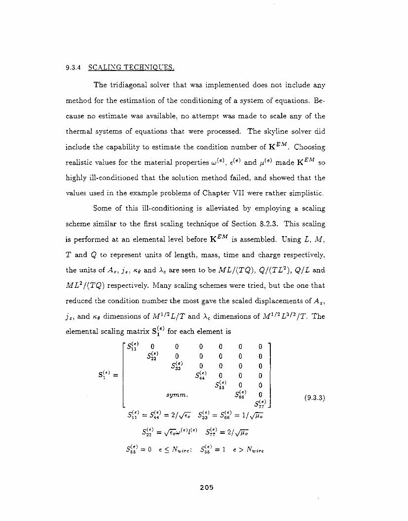
9.3.4 SCALING TECHNIQUES.
The tridiagonal solver that was implemented does not include any
method for the estimation of the conditioning of a system of equations. Be-
cause no estimate was available, no attempt was made to scale any of the
thermal systems of equations that were processed. The skyline solver did
include the capability to estimate the condition number of gEM. Choosing
realistic values for the material properties w (e), e(e) and #(e) made gEM so
highly ill-conditioned that the solution method failed, and showed that the
values used in the example problems of Chapter VII were rather simplistic.
Some of this ill-conditioning is alleviated by employing a scaling
scheme similar to the first scaling technique of Section 8.2.3. This scaling
is performed at an elemental level before gEM is assembled. Using L, M,
T and Q to represent units of length, mass, time and charge respectively,
the units of A=, jz, _0 and Ac axe seen to be ML/(TQ), Q/(TL2), Q/L and
ML 2/(TQ) respectively. Many scaling schemes were tried, but the one that
reduced the condition number the most gave the scaled displacements of A:,
jz, and _0 dimensions of MI/2L/T and Ac dimensions of M1/'2"L3/2/T. The
elemental scaling matrix S_ _) for each element is
S_') =
0 0 0 0 0
0 0 0 0 0
s_ _ o o o os2 _ o o o
s_? o osymm. s__ o
s_?= s;:?= 2/,/770
s_;_= ,/_:._'_l_°_
s__= o __<N_,,0;
s_?= s_;_= 1/,/-_;
s_?= 2/,/'#7
S[[ ) = I e > Nwi,-,
(9.3.3)
205

-(*) -(_) The inclusionof the elementalwhere I(¢)isthe elemental length .j - ri .
length in the scalingparameter for jz does not cause any difficultiesbecause
the only diagonal terms affectedby S_ )of K EM correspond to the jz degrees
of freedom which do not couple through the diagonal terms.
To illustrate this point, consider the diagonal terms corresponding to
the degrees of freedom for Az of a two element system that contains a total
of three element end nodes. If A(2 ) is scaled for each element by/(*), A(__) at
the shared center node will be scaled on an elemental level by l (1) for the first
element and l (2) for the second element. Note that the bracketed superscript
numbers represent the element number and not an exponent. This causes
no problem in determining scaling factors if l (1) equals l (2). It is simply
l (1) or l (2). But if the lengths differ, problems will occur because A_ at the
shared node will be scaled into two different dimensions! Trying to assemble
the scaled elemental diagonal terms of A_ with this scaling would result in
an error because each scaled variable represents a single scaled independent
variable.
The scaling matrix of(9.3.3) avoids these difficulties due to a careful
choice of its elements. ¢(e)"_55 ensures no coupling of adjacent values of j_') and
also ensures that there are no zero diagonal terms of the assembled scaling
q(e) alsomatrix for degrees of freedom of j(_') that are constrained to zero. "-55
ensures that no zero diagonal term appears for the extra "empty" degree of
freedom of K EM that is discussed in Section 7.3.
206

The scaled elemental electromagnetic tangent stiffness matrix for
1 < e < Nwi,-e is
-(_) 0 0 0 0 0
-(_) 0 K2_ K27--r(m*) K23 '-j
o o0 0 0 0
0 0 0
syrnrn, r_ ) 0
0
(9.3.4)
l (*) #oco r_ ) _/(*)/6 /(2s =I(23 = 2 _(*) 2 w(*)
l (_) _oCo r_ )K27 = 2 w(_)
where r_ ) = (!/2)(rl_) + r(-_))is the mean radius of the element and coJ J
is the speed of light in vacuum. As can be seen by inspection, the closer
(I(*)/2)(#oCo/w (_)) is to one, the better the conditioning of the matrix. If
this occurs, it can also be seen that all of the terms become proportional
to approximately r_)//(_). Using the test material of high purity aluminum
does not allow (l(e)/2)(#oco/w (_)) to come as close to one as is desired, and
other means are used to reduce the conditioning of the scaled electromagnetic
system of equations. It was found that the choice of mesh discretiztion
greatly affected the conditioning of the system, and this is the next topic of
discussion.
207

9.3.5 MESH GENERATION.
The thermal conduction problem is similar to the superconductivity
problem because a finer mesh discretization is required near rc to accurately
determine the nodal values of the independent variables. The independent
variable for the thermal conduction problem is 7" and the electromagnetic
quantity w in the temperature range of interest is proportional to its. This
behavior suggests that electromagnetic quantities vary either much more
quickly or more slowly than ir depending on whether the system is above
or below 1° Kelvin. This behavior also suggests the use of separate meshes
for the electromagnetic and thermal equations. Separate meshes were not
used for the examples of this work because they require a transfer of data
between the thermal mesh and the electromagnetic mesh and are subject to
extrapolation errors. Separate meshes also require more computational effort
and memory storage. For the above reasons, it was decided to use a single
mesh for both the linear electromagnetic and thermal system of equations.
As mentioned above, there is a finer grading of the thermal mesh at re. This
grading was determined to be a source of ill-conditioning for the assembled
EM equations.
Originally, a small region near rc was discretized with regular finite
elements and the remainder of the conductor volume was descretized with
larger regular finite elements. It was seen that at the node where the two
meshes joined, off-diagonal terms were generated that were substantially
larger than diagonal terms. Other off-diagonal terms that were substantially
smaller than diagonal terms were also generated. To cure this problem, the
scaling scheme of the previous section is used to make off-diagonal terms of
208
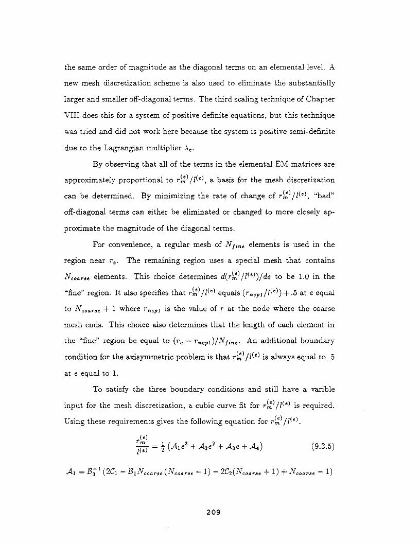
the same order of magnitude as the diagonal terms on an elemental level. A
new mesh discretization scheme is also used to eliminate the substantially
larger and smaller off-diagonal terms. The third scaling technique of Chapter
VIII does this for a system of positive definite equations, but this technique
was tried and did not work here because the system is positive semi-definite
due to the Lagrangian multiplier _c.
By observing that all of the terms in the elemental EM matrices are
approximately proportional to r_)/l (e), a basis for the mesh discretization
can be determined. By minimizing the rate of change of r_)//(e), "bad"
off-diagonal terms can either be eliminated or changed to more closely ap-
proximate the magnitude of the diagonal terms.
For convenience, a regular mesh of N fin, elements is used in the
region near re. The remaining re#on uses a special mesh that contains
N, oar,_ elements. This choice determines d(r_)/l(*))/de to be 1.0 in the
"fine" region. It also specifies that r_)/l (*) equals (r,,cpl//(*)) + .5 at e equal
to Ncoar,, + 1 where r,_cpl is the value of r at the node where the coarse
mesh ends. This choice also determines that the length of each element in
the "fine" region be equal to (re - rncpl)/Nfm,. An additional boundary
condition for the axisymmetric problem is that r_)/l (*) is always equal to .5
at e equal to 1.
To satisfy the three boundary conditions and still have a varible
input for the mesh discretization, a cubic curve fit for r_)/l (*) is required.
Using these requirements gives the following equation for r_ )/l (*).
•,41 = _-1 (2Cl -- ]31_coarse(_coarse -- 1) - 2C2(Ncoar, e + 1) + Ncoarae - 1)
2O9
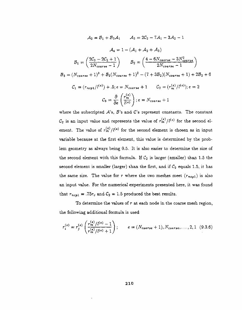
.2,2 --- B1 + B2.A1 .2,3 = 2C2 - 7.41 - 3.A2 - 1
A4 = 1 - (A_ + A2 + A3)
/33 = (Ncoa,-,e + 1) 3 + I32(Ncoar,_ + 1) 2 - (7 + 3B2)(N¢oa,.,_ + 1) + 2/32 + 6
cl = (T_cpl/z(*))+ .5;, = Nco,,,, + 1 ¢_.= (T_)/z(')); _ = 2
a (_)_,C3 = _ee \/-_J ,e= Nco_,s, + 1
where the subscripted A's, B's and C's represent constants. The constant
C2 is an input value and represents the value of r(_)/l(*) for the second el-
ement. The value of r_)/I (*) for the second element is chosen as in input
variable because at the first element, this value is determined by the prob-
lem geometry as always being 0.5. It is aaso easier to determine the size of
the second element with this formula. If C2 is larger (smaller) than 1.5 the
second element is smaller (larger) than the first, and if C2 equals 1.5, it has
the same size. The value for r where the two meshes meet (r,¢pl) is also
an input value. For the numerical experiments presented here, it was found
that r,,px = .75rc and C2 = 1.5 produced the best results.
To determine the values of r at each node in the coarse mesh region,
the following additioned formula is used
_.) _(.) -I)= -- ; e = (N,o:,-,, + 1),Nco,,-,,,... 2,1 (9.3.6)r, rj \r_)/;(. ) + 1
210

9.3.6 FIELD RECOVERY.
For the thermal part of the problem, the 7" field is recovered by
using the values of v "r. The electromagnetic fields are determined by using
the simple finite element approximation of Chapter V, Equation (5.3.6). This
value was plotted as a step function due to its C -I continuity.
9.3.7 TEST PROBLEM.
In this example, high purity aluminum was again used for the test
material. The values for k and _(e) were calculated as discussed earlier in
this chapter. The permeability and permittivity for all elements were set to
/1o and eo as explained at the beginning of Chapter IV. The reference state
for v was set as described in Section 9.3.3. The geometry was that of a
one-dimensional axisymmetric wire as shown in Figure 2.1 with a radius rc
transporting a total current I equal to 5 amperes in the positive z direction.
The mesh was discretized as described in Section 9.3.5 with rc equal to
1.15 × 10 -4, Ncoa,-s_ equal to 50 elements and dV/in_ equal to 30 elements.
This gave a total of 1¥_i,-_ equal to 80 elements. Because the element for
the free space magnetic fields had been validated before, no elements were
generated external to the conductor. The solution tolerance r was 9.0 × 10 -4
and required about 2 iterations per step to converge. The estimated condition
number for K EM ranged from 10816 to 65888. The initial temperature was
chosen as 10 Kelvin and the loading temperature was 1° Kelvin. The step
size In was chosen as .025 and 40 steps were necessary to move the solution
from the starting temperature of 10 Kelvin to 2 ° Kelvin.
The results for the analytical solution and the finite element solution
for 7" were so close as to be indistinguishable on a plot. Consequently, Figure
211

9.1 shows the results for the finite element solution for the temperature
distribution and Figure 9.2 showsthe percentageerror of the finite element
solution from the analytical solution as functions of the radial distance at
the final step (Too= 2° Kelvin). A comparison of the Euler equations of the
EM problem (Equation (2.3.11))and the thermal problem (Equation (4.1.8))
shows that they are of an identicalform. If/¢isnearly constant and w(_)j!e)//¢
approximates a constant, then the behavior of Az and ir within the example
wire should be the same. A comparison of Figure 9.1 with Figures 5.2 and
7.2 show that thisis indeed the case. Figure 9.2 shows the deviation of the
computed solution from the analyticalsolution as a percentage error,and it
ranges from a maximum at r = 0 of 2.860 x 10⁻³ to zero at r = r=.
The primary variablesof interestfor thisresearch were the B fields,
and they are the only EM resultsthat are shown here. Figure 9.3 and 9.4
show the resultsfor the Be fieldat the finalstep. Figure 9.3 shows the B0
fieldover the whole conductor and Figure 9.4 shows the B0 fieldfor the
volume of the mesh with the finerdiscretization.The percent error ranged
from 33.1 percent at r = 0 to 5.89 x 10⁻⁴ at r = re. By observing where
the analyticalsolution intersectsthe '_steps"in Figures 9.3 and 9.4,a rough
estimate of the accuracy of the finite element solution can be made. The finite
element solution is exact when the analytical solution intersects the center
of the "step tops". It can be seen that the analytical solution intersects the
majority of the "steps" at their center points. It can also be seen that the
error quickly diminishes as the distance from the center of the conductor
increases.
As mentioned earlier,the solution procedure isnot exact. Also men-
tioned was that the exact solution can be computed by settingTo to the full
212

T
e
m
Pe
ra
tU
r
e
2.089
2.081
2.073
2.065
2.057
2.049
2.042
2.034
2.026
2.018
2.210
0.000 2.300 e-5 4.600 e-5 6.900 e-5 9.200 e-5 1.150 e-4
Radial Distance
Figure 9.1:T vs. r, values for the finiteelement solution plotted.
3.00 e-3
2.70 e-3
Pe 2.40 e-3
r2.10 e-3
C
e 1.8o o-3n
t 1.50 °-3
E 1.20 °-3
rr 9.00 °-4
O6.00 e-4
r
3.00 _-4
0.000 ' I r
0.000 2.300 °-5 4.600 e-5 6.900 e-5 9.200 e-5
Radial Distance
I
1.150 e-4
Figure 9.2: Percent error of the finite element solution from the analyticalsolution for T vs. r.
213

load, TL to zero and using the correctiveNewton-Raphson method to iterate
onto the equilibrium path.
The above technique was triedfor thisnumerical example and itwas
found that the f_uiteelement resultspresented here differedfrom the exact
solutionby 4.68× 10⁻² and 3.43× I0-s percent for the temperature at r equal
to zero and r¢ respectively.The B0 fielddifferedfrom the exact solution by
33.3 and 8.60 × 10⁻⁴ percent at r equal to zero and rc respectively.
A briefword must be said here about the analyticalsolution of Sec-
tion 9.2. In general,the analyticalsolutiondoes not match the exact solution
because ituses the nodal values of T from the previous step to compute k,
_(e) and j(_).The analyticalsolutiononly becomes the exact solution when
_T isheld constant and the solution isallowed to iterateonto the equilibrium
path. This brings about the rhetoricalquestion, why bother computing the
analyticalsolution?
The analytical solution is computed because it gives some measure
of how close the finite element solution is to an exact solution. It will always
give the correct form of the solution, but not the correct ma=cmitude if the
solution lies close to the true equilibrium path. This is the first step in
assessing the accuracy of the solution vector produced by the non-linear path-
following techniques used in this work. The second step is to hold the ioading
parameter constant and then use the corrective Newton-R_phson technique
to iterate to the exact solution. The exact solution is then compared to the
original incremental solution. If the difference between the two solutions is
too large, then the solution procedure has moved too far from the correct
equilibrium path and a smaller step size needs to be chosen. The solution
process is attempted again with the new step size and _ reset to zero.
214

B
Fi
e1
d
0.008
0.007
-0.007
0.006
0.005
0.004
0.003
0.002
0.001
8.69566 e-4
0.000
0.000 2.300 e-5 4.600 e-5 6.900 e-5 9.200 e-5
Radial Distance-- Finite Element
.... Analytical
1.150 e-4
Figure 9.3: Be vs. r, values for complete mesh plotted.
B
Fie1d
0.008695
0.008143
0.007590
0.007038
0.006485
8.62500 e-5
fJ
I I I
9.34376 e-5 1.00625 e-4 1.07812 e-4
Radial Distance-- Finite Element
.... Analytical
1.15000 e-4
Figure 9.4: Be vs. r, values for finer discretization plotted.
215

In general, it is not possible to hold the loading parameter constant
at its final value and iterate onto the exact solution without first following the
incremental path to that point. There may be bifurcation points or other
stationary points on the equilibrium path that will not allow the solution
method to converge to the correct solution by this simple iterative process.
The problem of the thermally loaded conductor presented here does allow
the above method to converge because it can be determined where the only
critical point for this problem lies, that point being the superconducting
phase transition point.
The plots for T and Be presented here show that with an appro-
priate mesh choice, a reasonable step size and a slowly varying temperature
distribution that the solution technique presented here is adequate for the
author's purposes and little accuracy is lost with this solution procedure.
9.4 SUMMARY.
In this chapter, it is shown how thermal fields may be modeled with
the LINT1D finite element. The CUPLE1D finite element is also adapted
to the nonlinear solution techniques of Chapter VIII to become the LET1D
element. This demonstrates the usefulness of the four-potential method and
the solution techniques for modeling the coupling that occurs between ther-
mal and EM fields. The four-potential theory is also validated for computing
the desired EM quantity, the B fields and the effects of temperature on these
fields by the results presented in this chapter. The use of real values for w, #
and e make the problem more difficult to solve, but by using a different mesh
discretization and scaling techniques, good solutions for the B field can still
be realized.
216

For this chapter, the case where only thermal loads are allowed to
vary is solved. In the next chapter, the case where the EM load I is allowed
to vary is examined.
217

COUPLED THERMAL-EM PROBLEM IN NORMAL CONDUCTOR
In the previous chapter, the consequences of varying the ther-
mal loading on a conductor are discussed. In this chapter, the thermal-
electromagnetic coupling in a normal conductor loaded by varying the cur-
rent I is discussed. Most of the necessary ground work to consider this
problem is developed in the previous chapters. Analytical solutions to both
problems are discussed in previous chapters and are not presented here. The
solution, mesh discretization and scaling techniques of the previous chapter
are also implemented for the varying current load problem. The only parts of
this problem that change are parts of the LINT1D finite element that depend
explicitly upon j, which is a function of the current load I, and the parts
of the LETID finite element that are dependent upon I. The first topic of
discussion is the modification of the LET1D finite element to include cases
where I is allowed to vary.
10.1 FINITE ELEMENT DISCRETIZATION.
10.1.1 MODIFICATIONS TO THE LET1D FINITE ELEMENT.
The first step in adapting the LET1D finite element for a varying
current load is to split I into an initial current Io and a loading current [L
as was done for the superconductor. Thus I = Io + _EMIL, where _EM is
the electromagnetic loading parameter. By using the Kronecker delta with
218

the boundary terms, the new equality for I, and Equation (7.2.2), f(e) p(,)
and v (e) are expressed as
f(e)= {KU(") + K*(*)} v(,) (10.1.1)
K *(`) = 2=H
0
j?)
v (_) = _)j0
A(_) j
_(1) ,(1) 0
0 0
0
0 0
-6m,r_m)w (m) 00 0
0 0
_me
syrnrn.
61ell
0
0
p(e)__ (Io + cEMIs) 0
0
0 O"
0 0
0 0
0 0
0 0
0 0
O.
(10.1.2)
(10.1.3)
where m again equals N_,_, + 1 and H represents the element height. The
matrix K *(*) is used here to add the boundary terms for _: to K (e) discussed
in Section 7.2.2. K *(*) also removes the rank deficiency generated by the
"empty" degree of freedom discussed in Section 7.3.2. The correct value of
K u(e) is given by Equations (7.2.3), (7.2.4), (7.2.5) and (7.2.6). Taking the
partials of f(e) and p(_) with respect to the independent variables contained
in v (*) gives the tangent stiffness matrix and loading vector, respectively.
Therefore the tangent stiffness matrix K (e), the loading vector q(e) and the
219

incremental rate vector w (e) are:
K (*) = K u(') + K*(*);
0
q(*) = IL 0
0
-6_,H
c3_ *)
cOj(*)
OA(*):
• w(*) = (:9_ _)
'0
0A(= e) .
(10.1.4)
It can be seen that K (e) is exactly the same as the stiffness matrix, modified
for boundary conditions and the extra "empty" degree of freedom of Chapter
VII thereby justifying the statement at the end of Section 7.1.1 that the two
are equivalent. A word of caution is necessary here because the expressions
for p(*) and q(e) are only valid for cases where the first degree of freedom for
Az is constrained. For the examples presented in the sequel, this is always
the case and no further information is needed to solve the EM system of
equations except that the "empty" degree of freedom for the fifth element of
v (m) must also be constrained to zero as explained in Section 7.3.2.
220

10.1.2 MODIFICATIONS TO THE LINTID FINITE ELEMENT.
The expressions derived in Chapter IX for K _r,p_r and fm for the
LINTID finiteelement do not depend upon the current load f explicity
and may be used without modification to solve the current loading problem.
Because p(e) for the LINTID element does contain j_e),it must be varied
with respect to the loading parameter _EM to determine what happens to
the thermal system of equations as f is varied. The resultfor q(')is
_j(e) r
The assembled system of coupled thermal and EM equations with this form
for q can be expressed as
K EM0
0
KT] IwEM qEMw.}:{,.)<,o.,.o,where qT is now a function of w EM . This form of the equations is undesirable
because terms of the incremental rate vector appear on both sides of the
equality sign. Moving qtr to the left hand side produces
o]{w..}{+.}K EMq" K T w T = 0 (10.1.7)
where K EMT" contains the elements of _q:r at the appropriate positions.
This form of the equations is also undesirable for two reasons. First,
the extra matrix K EMT must be assembled which requires more computa-
tional effort and memory storage. It also ruins the sparsity and the symmetry
of the original system of equations and a tridiagonal solver can no longer be
used to process the thermal equations. Second, K EM'I- is also a function of
the independent variable j_.. This affects adversely the conditioning of the
221

coupled system and typically requires more iterations to converge upon a
solution than a set of linear equations, which only requires a single iteration
to converge.
If the form of Equation (10.1.6) is preserved by making q:r a function
of [EM, the original sparsity of the system is retained and computational
effort and memory storage are reduced. To accomplish this goal, Equations
(7.1.2) and (7.1.3) are used. Insertion of (7.1.3) into (7.1.2) gives
N.j;,e
- Zo+ eE.ZL=Ip=1 i ') w(_-'-'_ (10.1.8)
where the superscripts (p) and (e) again represent element numbers and
Nwi_, is the total number of elements within the conductor. Rearranging
Equation (10.1.8) and taking the partial of j(e) with respect to (EM gives
OJ_) 1 { IL } (10.1.9)
The bracketed term of the above expression is evaluated when assembling
gEM and requires less computational effort and memory storage than the
scheme presented in Equation (10.1.7). The thermal loading vector q_" is
stiff a function of the EM solution vector V EM but does not cause difficulties
in the example problems. The value of V EM at step n is used to compute w
at step n + 1 in the same manner that v T is used at step n to compute k
and w for K _ and K EM at step n + 1.
The coupled system of thermal and EM equations is conservative
and the variation of the discretized functionals that describe this system
should produce a symmetric system of equations. The fact that (10.1.7) is
222

not symmetric iscaused by the use of approximations that render them in-
complete. In Chapter IX_ itisassumed that j isonly a function of f but not
of the temperature T, an approximation responsiblefor the unsymmetry Of
(10.1.7).This point ismentioned here to emphasize the importance of using
the nonlinear solution procedure of Chapter VIII and equilibrium path fol-
lowing procedures to generate correctsolutions.For small incremental steps,
the methods described in thisand the lastchapter work wellfor determining
solutionsfor the coupled system of thermal and EM equations although the
complete set of equations is not solved. Because the solution never moves
too far from the equilibrium path, the missing terms have littleeffecton
determining a correct solution.
10.2 NUMERICAL EXPERIMENTS.
10.2.1 THE FINITE ELEMENT MODEL.
The finite element model described in the previous section has been
applied to the in_nite axisymmetric normal conductor of the previous chap-
ter. The modifed LET1D and LINT1D finite elements are used to determine
EM qumatities and the temperature distribution, respectively. Both of these
elements are treated as one-dimensional axisymmetric two node "line" type
elements. The description of the nodal degrees of freedom and the vari-
ables associated with each degree of freedom for the LET1D element are the
same as the CUPLE1D element and are found at the beginning of Section
7.3.1. The permeability #, the resistivity _ and the current density j= are
all assumed to be uniform over each element.
223

For the modified LINT1D finite element, the description of the nodal
degrees of freedom and the variables associated with each degree of freedom
are found in Section 9.3.1. The material constants k and w are also deter-
mined by the same methods discussed in that section. The value used for
j(e) to determine q(*) at step n + 1 comes from the EM solution vector at
step n and Oj(*)/o¢EM for q(*) is determined by use of Equation (10.1.9).
The boundary conditions for this system are the same as described
in Section 9.3.2 and are set in the same manner.
10.2.2 ASSEMBLY AND SOLUTION.
The assembly and solution of the coupled EM-thermal normal con-
ducuctor with a variable current loading is identical to a conductor with
variable thermal loading except that Equation (10.1.5) is used to determine
q_'. The scaling techniques implemented for K EM for the thermally loaded
conductor are also used on K EM. The mesh generation and field recovery
techniques used here are also identical to the techniques of Sections 9.3.5 and
9.3.6 respectively.
10.2.3 TEST PROBLEM.
A one-dimensional axisymmetric wire made of high purity aluminum
was used as test example. The geometry is shown in Figure 2.1. The radius of
the wire rc is 1.15 x 10 -4. The wire transports a total current of Io + _EMIL
in the positive z direction where Io is zero amperes and IL is 5 amperes.
The free stream temperature of the system Too is held constant at 2 ° Kelvin
by setting the initial temperature To equal to 2 ° Kelvin and the loading
temperature TL equal to zero. The convection heat transfer coefficient hconv,
224
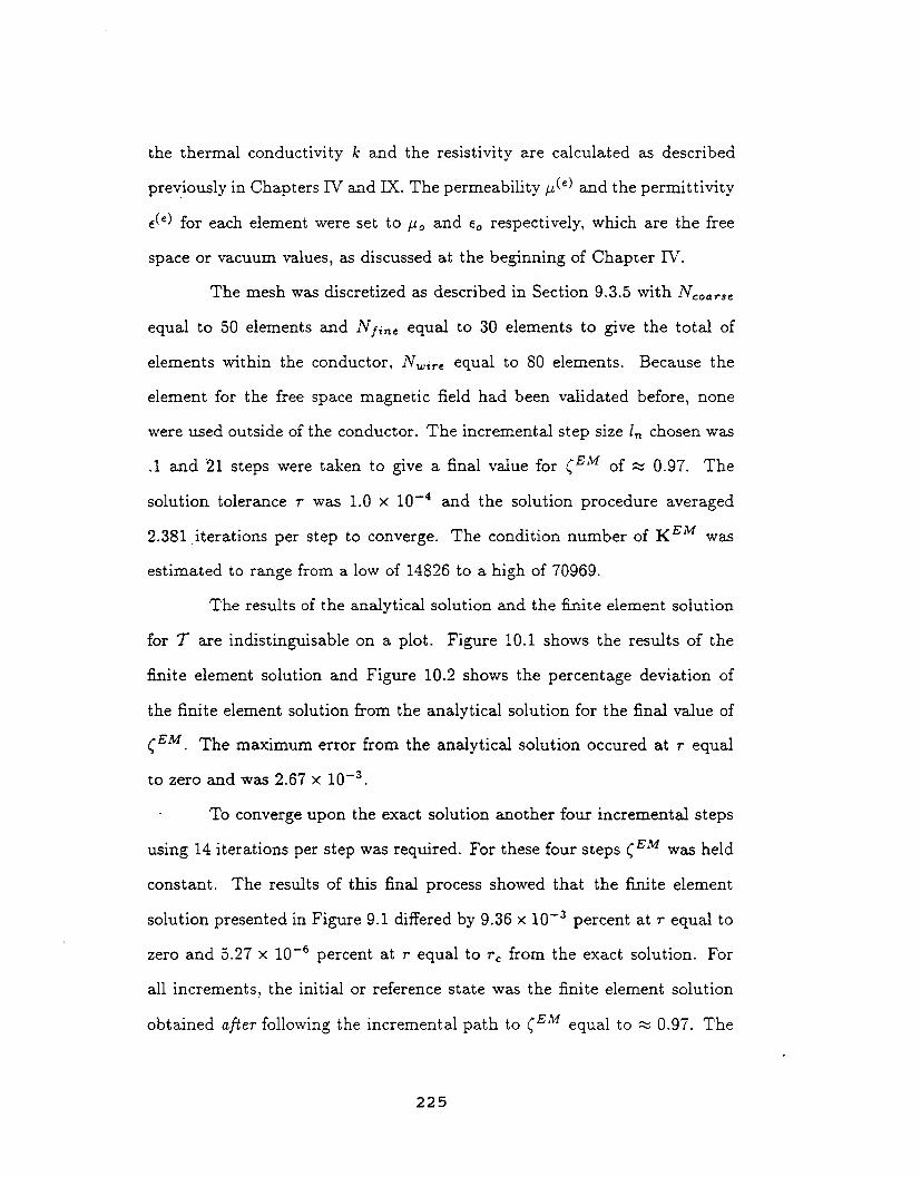
the thermal conductivity k and the resistivity are calculated as described
previously in Chapters IV and IX. The permeability #(e) and the permittivity
_(e) for each element were set to #o and _o respectively, which are the free
space or vacuum values, as discussed at the beginning of Chapter IV.
The mesh was discretized as described in Section 9.3.5 with Ncoa_se
equal to 50 elements and Nyine equal to 30 elements to give the total of
elements within the conductor, ]Vwire equal to 80 elements. Because the
element for the free space magnetic field had been validated before, none
were used outside of the conductor. The incremental step size l,_ chosen was
.1 and 21 steps were taken to give a final value for (EM of _ 0.97. The
solution tolerance r was 1.0 x 10 -4 and the solution procedure averaged
2.381 iterations per step to converge. The condition number of K EM was
estimated to range from a low of 14826 to a high of 70969.
The results of the analytical solution and the finite element solution
for T are indistinguisable on a plot. Figure 10.1 shows the results of the
finite element solution and Figure 10.2 shows the percentage deviation of
the finite element solution from the analytical solution for the final value of
(EM. The maximum error from the analytical solution occured at r equal
to zero and was 2.67 × 10 -3.
To converge upon the exact solution another four incremental steps
using 14 iterations per step was required. For these four steps (EM was held
constant. The results of this final process showed that the finite element
solution presented in Figure 9.1 differed by 9.36 x 10 -3 percent at r equal to
zero and 5.27 x 10 -6 percent at r equal to re from the exact solution. For
all increments, the initial or reference state was the finite element solution
obtained after following the incremental path to CEM equal to _ 0.97. The
225

state at _EM _ 0.97 was actually quite close to the equilibrium path. The
high iteration number required to move the solution back onto the equilib-
rium path illustrates the difficulty associated with finding an exact solution
by simply using the corrective Newton-Raphson process. Sometimes, direct
iteration is not possible or more expensive computationally than just using
the incremental "path following" solution method presented here.
Figures 10.3 and 10.4 show the finite element and analytical solutions
for Be. Figure 10.3 shows the two solutions plotted over the whole domain
of the conductor, and Figure 10.4 shows the solutions over the domain of
the finely graded mesh. At r equal to zero, B# differs from the analytical
and exact solutions by 33.3 percent. At r equal to re, Bs has errors of
5.91 x 10 -4 and 5.85 x 10 -4 perecent when compared to the analytical and
exact solutions respectively.
Although not mentioned until this point, the 33.3 percent error at
r equal to zero appears to be large. Subtracting out the temperature at r
equal rc from allof the finiteelement and analyticalvalues for 9" and then
recomputing the percent error for T willgive the same error at r equal to
zero of 33.3 percent. This observation has led the author to believe that the
error is the same for all systems of equations of the form _7. (aVb) = f(b)
when this system is modeled with finite elements. Here a represents some
material constant, b the independent variable, and f(b) some function of the
independent variable b. If the above observation is correct, it should always
be possible to correct any error when modeling a system of this form.
A quick look at Figures 5.3, 5.4, 7.3, 7.6, 9.3 and 10.3 shows that the
correction is probably unnecessary. The divergence of the computed solution
226

Te
m
Pe
rat
U
re
2. 083
2. 076
2.068
2. 061
2. 053
2.046
2. 039
2. 031
2. 024
2.016
2.009
0.000 2.300 e-5 4.60000 e-5 6.900 e-5 9.200 e-5 1.150 e-4
Radial Distance
Figure 10.1: 7" vs. r, values for the finite element solution plotted.
3. O0 e-3
2,70 e-3
Pe 2.40 e-3r
2. i0 e-3C
e 1.8o .-3n
t 1.50 e-3
E 1.20 e-3
rr 9.00 e-4
o6.00 0-4
r
3.00 e-4
0.000 I I. l '
0.000 2.300 e-5 4.600 e-5 6.900 e-5 9.200 e-5
Radial Distance
T
1.150 e-4
Figure 10.2: Percent error of the finite element solution from the analyticalsolution for 7- vs. r.
227

from the exact solution is so small as to be almost unnoticeable and from a
practical engineeringstandpoint, the error is not noticeable.
The reasonthat the 33.3percent error appearsto be large is because
the computed solution is comparedto the exact solution on a node to node
basis. This is formally expressedas
% e_o_= BpE(_)-SEx(_)× lO0 (I0.2.1)SEx(r)
where BFE and BEX are the finiteelement and exact values respectivelyfor
the Be Keld. A more realisticerror estimator for engineering purposes is
%err_ = BF_(r) - BEx(r) × 100 (10.2.2)Bsx(_) + SEx(re)
This type of error estimate has been used to compute the error for T in
this and previous chapters. %Vhen computing "7" on a node by node basis,
the boundary loading has already been factored into the estimator. The
conclusion of thisbrief digression is that an error estimator by itselfis not
always a good indicator of the accuracy of a finiteelement model. Graphics,
a relationshipof numerical answers to the actual physics of a modeled prob-
lem and good en_neering common sense should all be used with an error
estimator to judge the validityand usefulness of each finiteelement model.
10.3 SUMMARY.
In this chapter, a form of the LINT1D finite element is derived for the
case where I is varied instead of T. The LET1D finite element is modified,
and using a nonlinear solution technique it is possible to compute some good
values for the thermal and magnetic fields of a one-dimensional axisymmetric
conductor.
228
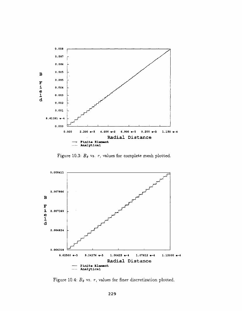
B
Fie
1d
0 .oog
0. 007
0.006
0. 005
0. 005
0.004
0.003
0.002
0.001
8.41181 e-4
0.000
0.000
I 1 I I 1 t
4.600 e-5 6.900 e-5 9.200 e-5 1.150 e-4
Radial Distance
2. 300 e-5
-- Finite Ele_ent
.... Analytical
Figure 10.3: Bo vs. r, values for complete mesh plotted.
B
Fie
1d
0.008411
0.007886
0.007360
0.006834
j/
0.00G308 , I I I
8.62500 e-5 9.34376 Q-5 1.00625 e-4 1.07812 e-4
Radial DistanceFinite Element
.... Analytical
1.15000 e-4
Figure 10.4:B0 vs. r, values for finer discretization plotted.
229

This represents the next to the last phase of this work's analysis of
the coupled quantum phase-EM-thermal problem for superconductors. It
is now possible to generate models of the superconducting material in its
normal and superconducting phases. It is also possible to determine the
ei_ect of varying either the thermal 7" or current J" loading of that material.
The next chapter is concerned with the use of the final versions of
the LINT1D and LETID finite elements with the STEP1D finite element
in a single computer program. This program is used to determine the cor-
rect state of a superconducting material and the values of the thermal and
magnetic fields.
230
THE COMPLETE COUPLED PROBLEM.
This chapter is concerned with the correct application of the LINT1D,
CUPLE1D and the STEP1D finite elements to the the specific problem of
determining the electromagnetic and thermal fields wi thin a superconducting
material. The main limitation on this model is that it is only one-dimensional
and cannot realistically model the state where B and T reach their critical
values because, as noted previously, the solution at the transition state is a
multi-dimensional problem. At this bifurcation point, a mLxed normal and
superconducting state appears that needs to at least include var/ations of
¢ in the z direction to obtain an accurate model of the physics that occur
within a conductor [21, pp.99-103; pp.127-1911. This point Mso marks where
the computed solution must change equilibrium paths to accurately model
the physics of the electron transport within a conductor.
The methodology required to model a superconductor when the ther-
mal loading is varied is first discussed in some detail. Then the question of
how to determine if a computed solution lies above or below the bifurcation
point is discussed. Means to determine whether or not such a solution is
correct axe also presented. These means form the basis of an equilibrium
path changing criteria. Finally, results that show the model changing state
as I and Too are varied axe presented to validate the path changing criteria.
231

11.1 A SUPERCONDUCTOR WITH A VARYING 9" LOAD.
To use the incremental approach to solve the superconductor with
a varying thermal load, f_M and pEM are varied with respect to v _r and
(_'. The thermal quantities f_" and p_" are also varied with respect to v sM.
Doing so produces a system of incremental equations that can be partitioned
in the following manner:
gEM KEMT
where K sM and K _r are the previously derived tangent stiffness matrices for
the superconducting and thermal conduction problems respectively and q:r
is the previously derived loading vector for the thermal conduction problem
with convection boundary conditions. The matrix K EMT is 69fEM/cgvT and
the zero entries on the left and right hand sides of the equality sign appear
because oqfT/onv EM "- Oand cgqEM/og_T -- 0. Because the resistivity of each
element w (e) is zero for a superconductor, only one nonzero term appears in
q_'. This term has a magnitude of 3-L and appears at the degree of freedom
for 3- associated with the radial distance re.
Solving the set of thermal equations produces the simple result that
3- is a constant over the whole conductor, the value of 3- at each node being
equal to To + ¢,7"+lTl,. This simplifies the solution procedure considerably
because the thermal equations KT"w 7" = qT', need not be solved by assem-
bling and inverting K _r. Instead of solving (11.1.1), which also requires the
assembly and storage of K EMT, the corrective Newton-Raphson technique
is used to directly iterate to a solution for V EM. This is accomplished by
solving the superconductor problem with the current load I held constant.
The value for T at each node is the value oft at the n+l step, To + _+13-L,
232

where _r_n+_ equals _+ In and the quantity l_ is the input step size. This is
the value of ir that is also used to determine _ and _, since they are both
functions of T and their values are required to obtain the correct EM tangent
stiffness matrix K EM.
Essentially this is the same incremental/iterative solution method
used in the two previous chapters to generate the exact solutions for T (e),
j(e) and A (e). The loading parameters (EM and (_r are held constant and
the system is allowed to iterate onto the equilibrium path. As mentioned in
those chapters, this technique can fail or become computationally expensive
when a large number of corrective iterations is required. Early in the testing
of the STEP1D element, it was observed that a reasonable solution for I@t (_)
and A! e) could be obtained in this manner if the reference state is set so that
all unconstrained values of equal to l ool and all values of are
set equal to zero. The number of iterations needed for convergence with
this reference configuration was usually less than ten. This configuration is
also identical to the initial reference state that is used to start the solution
procedure for a superconductor when the current loading I is varied. This
means that the subroutine that generates the initial reference state for the
varying current problem can also be used to generate a reference state for
the varying 9" problem thereby reducing the logic and memory requirements
of a code that solves both problems.
The computational cost of using the above solution method is that
more iterations are required at each step and the reference configuration must
be recomputed at each step. There is also no guarantee that the solution
method will convege but numerical experiments strongly suggest that it will.
233

The corrective Newton-Raphsontechnique is therefore usedto solve
the problem of a superconductor with a varying thermal boundary load for
the following reasons:
I. Assembly and storage of K EMir is unnecessary.
2. The number of iterationsrequired per step isrelativelymodest.
3. Convergence, as determined by numerical experiments, always occured.
4. The referencestate isidenticalto the initialconfiguration of the I load-
ing problem, allowing the use of one subroutine to set eitherconfigura-
tion.
11.2 DETERMINATION OF THE CORRECT EQUILIBRIUM PATH.
To check whether the conductor is in the normal or superconducting
state, one determines the critical temperature _ and the critical magnetic
field Be. Then Bc and Tc are compared to the largest magnitude of B and the
highest temperature T (typically Too) field within the conductor. If either
or Bc is exceeded, a superconductor changes quantum states and becomes a
normal conductor. This change of state occurs because at 'T" equal to Tc or B
equal to Be a bifurcation point for the equilibrium paths of a superconductor
and a normal conductor exists.
The existence of this bifurcation point also means that if the con-
ductor is originally in the normal state and Too falls below _ and the largest
value of B within the conductor is less than Be, the material becomes su-
perconducting. It is therefore important to know the values of _ and Bc so
that the position of the bifurcation point along the equilibrium path can be
determined. The critical temperature :To is a material constant, and is de-
termined either by experimentation or by referencing previous experimental
234

data. The critical B field Bc is determined by using Equation (4.4.1) which
is a function of the temperature iT.
An alternative method for finding the correct conductor state is
to compute the Helmholtz free energyfor the superconducting and normal
states of a conductor for the samethermal and current loading conditions.
After finding the free energiesof both systems,the state of the system can
be determined by choosingthe system that has the lower free energy. This
approachis computationally inefficient becauseit requiressolving for the de-
greesof freedom v of both states at every incremental step. It also requires
knowledgeof the heat capacity of the material for the superconducting and
normal states of the material, and finding thesevaluescan be a task of con-
siderable difficulty becauseof the dearth of experimental data. The first
approachis therefore chosenhere.
Following the first approach,the B fields and 7" distribution as de-
termined by v_+1 are checkedat the end of each incremental step to see
if they are sufficiently small so that a superconducting state is possible. If
that is the caseand the system was originally in the normal state at step
n, then V,+l is solved for again at step n + 1 using the superconducting
finiteelement STEPID. Ifthat isnot the case and the condutor was in the
normal state at step n, then the solution at step n + 1 is accepted and the
program proceeds to the next step keeping the normM conducting state ele-
ment LETID. Ifthe B fieldsand the T distributionare small enough at step
n + 1 and the system was originallyin the _zperconduct{ng state at step n,
the solution vector v,_+1 isaccepted and the solution process moves to the
next step using the STEPID finiteelement. Finally,ifeitherof the two fields
are too large for a superconducting state to exist,then vn+1 is recomputed
235

using the LET1D finite element and the solution method moves to the next
step using the LET1D finite element.
For the one-dimensional problem, this methodology appears to be
optimal and is the one used for the present numerical experiments. It has
the key advantage that knowledge of the heat capacity of the material is
unnecessary. Furthermore, the solution vector v only needs to be computed
twice when the system changes state. If the second path determination
method that involves computing the Helmholtz free energies of the normal
and superconducting states is used, the solution vector v must be computed
twice at ever v step.
The first approach naturally delineates the tests for the proper equi-
librium state of the system into four separate cases where a change of state
may occur. These cases are:
1. System originally in the superconducting state, thermal load increasing.
2. System originally in the superconducting state, current load increasing.
3. System originally in the normal state, thermal load decreasing.
4. System originally in the normal state, current load decreasing.
For cases where the system is originally in the superconducting state
and the current or thermal loading is decreasing, the system remains in
the superconducting state because the solution is moving away from the
bifurcation point and no problems involving equilibrium path chan_ng are
posed. Similarly, when the system is originally in the normal state and the
current or thermal loading is increasing, the solution remains in the normal
state because it is moving along the normal state equilibrium path away
from the bifurcation point. Again, this poses no problems to the solution
procedure.
236

The comparison of _rc to Too, the first path changing criterion, is rela-
tively straightforward and only involves the computation of T_ at each step.
The second criterion can cause problems. This criterion states that B for
every element of the conductor must be below Bc for a superconducting state
to exist. Comparing B over each element to Bc can become computationally
expensive as the number of elements used to model a problem increases. This
computational expense can be reduced by finding a priori where B attains
its largest value within the conductor. For the one-dimensional axisymmetric
infinite conductor, B attains its largest value at rc. A cursory examination
of Equation (5.1.8) verifies that the preceding statement is correct. Equation
(5.1.8) can also be used to determine that
#ol (11.2.1)
where #o replaces # for example conductors of this work, as discussed in pre-
vious chapters, and fr J" ficdF is equal to f. By using this analytical solution
for Be(re), a simple means exists for determining if a superconducting state
is possible.
The only situation not discussed so far is when the incremental solu-
tion falls directly upon the bifurcation point. As explained previously, at this
point the physical solution cannot be modeled by one-dimensional elements
and the LET1D element is used to model EM quantities although the solu-
tion generated does not represent the correct physical state of the system.
This method is used so that the solution method can proceed to the next
step without failing. The LET1D element does not fail at this point because
it is based upon a potential energy formulation. The STEP1D element fails
because it is based upon the difference of the Helmholtz free energies of the
237

superconducting and normal states. At the bifurcation point, this difference
is zero and the tangent stiffnessmatrix K EM becomes singular.
The physical significanceof what isoccuring isthat both the normal
and superconducting statespossess the same energy. In the actual physics,
a variation of _#occurs in the z direction,and the system chooses the eigen-
state that possesses the lowest possible energy and entropy. To extend the
current superconducting model to this problem, an adaptive mesh appears
to be necessary to determine the boundary between parts of the conductor
that are normal and superconducting. The adaptive mesh isalso required to
make K EM well-conditionedenough that reasonable values of Elvlquantities
can be generated by standard nonlinear solution techniques. Unfortunately,
time limitationson the thesisresearch precluded the development of an adap-
tive two-dimensional mesh and the examination of the physics of this most
interestingand challenging problem was foregone.
The STEPID finiteelement used for the thesisresearch should pos-
sess a rank deficiency of one at the bifurcationpoint. In an effortto gain
a better understanding of what was occuring at the bifurcationpoint with
the finiteelement model, the model was forced to converge upon this point
by setting the thermal loading to the criticaltemperature ir¢and setting
the current loading to a value that would generate the criticalfieldBc at
the outer conductor boundary r=. The correctiveNewton-Raphson solution
method was then used to iterateto the bifurcationpoint. The finiteelement
model actually converged and returned a quantum state that carried no cur-
rent and an applied external fieldof Bc at re. Even though K EM should be
singular at thispoint, a fact that precludes convergence, itis believed that
238

the STEPID model converged for two reasons. First,the CNR itera:ivepro-
cedure is stopped when the 2-norm of r issmaller than the input tolerance
_-. Second, the scalings and the factorizationof K EM introduce numerical
round off errors that perturb the generated solution off of the bifurcation
point just enough to render K EM nonsingular.
The STEPID model returned the resultof an applied external field
and no current in the conductor because it does not enforce the current
conservation constraint I - fr dFflc "J = 0. The addition of thisconstraint
automatically allows an EM model to distinguishbetween cases where the
fieldat rc isgenerated by a current I or by an externally applied B field.
The eigenvalue analysisof K EM for earlierversions of Ginzburg-Landau and
London superconducting finiteelements that contained the current conserva-
tion constraintshowed that the current conservation constraint isredundant
when no external fieldsare applied to the system or when v EM does not lie
upon the bifurcationpoint. These two cases are not considered in thiswork
and are not presented here.
To summarize, the basic path determination process isas follows:
A. Solve system of equations for v,+l.
B. Find T_ by using T_ = To + _[+ITL.
C. Find Bc at T_ by using Equation (4.4.1).
rEM rD. FindIbyusingI=/o+_ ,_+I_L.
E. Find B8 at rc by using Equation (11.2.1).
F. If Be(re) > Be, go to H.; if not, go to G.
G. If Too > To, go to H.; if not, go to I.
H. If the current EM element type is STEP1D, change it to LETID and go
back to A.; if it is not, go to 3.
239

I. Ifthe current EM element type is LETID, change it to STEPID, reset
the reference state of V EM and go back to A.; if it is not, go to J.
J. Accept solution vector v_+l for the current step.
Additional logic statements are included in the actual coding to help
prevent the STEP1D element from exceeding the bifurcation point. Beyond
the bifurcation point, the element will "zero in" upon the same type of solu-
tion that occurs when the element is forced to converge upon the bifurcation
point. A quantum state is generated where there is no current in the con-
ductor and a boundary Be field loading of magnitude (#of)/(2_vrc) exists.
This state usually requires more iterations to converge upon a solution and a
larger solution tolerance _- than physical states that lie below the bifurcation
point on the equilibrium path. Non-physical solutions for the superconduc-
tor that lie beyond the bifurcation point can also cause the CNR procedure
to fail if _" is too small or if the maximum number of allowed iterations for
the solution procedure is exceeded.
To prevent the STEP1D element from moving past the bifurcation
point and encountering these problems when the current load f is being
incremented, steps C through E of the path determination procedure are
performed prior to each corrector iteration. The current iteration value of
_EM+I is used for step D because the actual step size along the equilibrium
path may change with each iteration. If the step size changes, then _E_+ 1
changes for each iteration and so does the value of f. If Bc is exceeded at re
for any iteration, the program changes the element type to LET1D, and the
solution procedure restarts at step n and attempts to increment the loading
to step n + 1.
240

For the casewhere the thermal loading is varied, steps B through
E are performed prior to eachpredictor step. For this casewhere the tem-
perature 7" is being incremented, the current ! is held steady and causes no
problems because cEM is held constant and is known before the predictor and
corrector steps are taken. T is Mso known a priori as being To + (_+ ln)7.L
at step n + 1 as discussed in Section 11.1. Because 7[,_+1 is known before
the solution procedure begins, steps B through E of the path determination
process can be used to determine if the solution vector will move past the
bifurcation point before the solution process begins. Inserting this test before
the predictor step keeps the program from performing an unnecessary solu-
tion step. After steps B through E of the path determination process are
performed, Bc(T,+I) and T_ are compared to B0(rc) and T,_+I respectively.
If either of the two latter quantities exceed their critical values the EM el-
ement type is changed to LET1D and the solution procedure is allowed to
continue. If the critical values are not exceeded, the solution procedure is
allowed to continue unaffected.
11.3 NUMERICAL EXAMPLES.
The LINT1D, LET1D and STEP1D finite elements derived in previ-
ous chapters have been applied to the solution of the test problems described
later in this section. The CUPLE1D and STEPID elements were used to
determine EM quantities and the LINT1D element was used to determine
the thermal distribution for the normal state of the superconductor. The
temperature of each node of the superconductor is calculated as described in
Section 11.1 of this chapter. The description of the nodal degrees of freedom
and the calculation of the material properties of each element may be found
241

in their respective chapters. The application of boundary conditions, scal-
ing techniques, mesh generation techniques and the assembly and solution
techniques are also described in the respective chapters. For the graphical re-
suits generated in this chapter, B0 was calculated by using the integral form
of Maxwell's inhomogeneous equation for magnetic fields, Equation (7.1.5).
This equation requires knowledge of j(:*) to determine Bo. For the super-
conducting phase, j!e) is calculated by using Equation (3.2.16) and for the
normal phase j(e)iscalculated by using the elemental values returned in the
solution vector v. The integralof Equation (7.1.5)is evaluated by 2 point
Gaussian integration.
11.3.1 PROBLEM h VARYING T LOAD.
For this problem and the next, the test material is high purity alu-
minum. Reference and initial states of the system are set as described in
previous chapters. The geometry is that of a one-dimensional axisymmetric
wire as shown in Figure 2.1. The wire radius r c is 1.15 x 10 -4 meters and
transported a total current I in the positive z direction. The initial current
Io is 1 ampere and the loading current IL is 0 amperes. The initial free
stream temperature is .5625 ° Kelvin and the loading temperature I L is 1°
Kelvin. Because the free-space magnetic field element has been validated
previously, all elements are within the wire. The mesh for the superconduct-
ing phase has 98 elements in the boundary layer and 2 elements in the bulk
layer while the mesh for the normal phase of the conductor has 50 elements
in the coarse mesh and 50 elements in the fine mesh. As in Chapters IX
and X the depth of the fine mesh was .25 rc for the normal conductor. The
depth of the boundary layer mesh for the superconducting phase varies with
242

temperature asdiscussedin Chapter VIII. The stepsize I,_ischosen as .0125
and 80 steps are used to increment _ir from 0.0 to 1.0.A solution tolerance
_-of 4 × 10-17 isused for the superconducting state and 9 x 10⁻⁴ isused for
the normal state.
The solution procedure required 41 steps in the superconducting
phase averaging 4.61 iterationsper step. The estimated condition number
for these steps ranges between 181 and 834. The solution procedure then
required 39 steps in the normal phase with an average of 2 iterationsper
step. The estimated condition number variesbetween 29861 and 204664.
Data output filesfor allof the figuresto be shown for a11examples
in this chapter are saved every tenth step and allgraphical representations
of this data are labeled with the appropriate values of _r or _EM when
it was possible. Graphical representations of each data set are generated
by using the PLOT2D utilityto produce a raster fileand then using the
rasterfilesto create a PostScript language file.This is mentioned because
the graphical representations of data sets are subject to the limits of the
PLOT2D utility.The data sets for each variable were then loaded into a
singlefile,and PostScript language commands were used to generate a_xes
and data set labels and legends. This is mentioned for researchers who
wish to duplicate the graphical resultsbecause the PLOT2D utilitydoes not
possess the abilityto add the desired labelsand font types or graph I0 sets
of data on a singlegraph.
Results for the temperature distributionwithin the wire are shown
in Figure II.I and match the expected physical behavior. The resultsfor
I_bl2/l_b_I2 in the region 1.023 x 10⁻⁴ _< r _< rc are presented in Figure
11.2. The value of the normalized value of l_blisnot shown over the whole
243

conductor because all of the physics of interest occured within the boundary
layer. The value for t_bl2/1¢_12 for r in the region 0 _< r < 1.023 x 10 -4 is
a constant equal to 1.0. The expected physical behavior for the normalized
value of [¢[ in the boundary layer was that as the temperature increased,
the boundary layer depth would increase mad [_bi2/[¢oo[ _ would vary over
a wider range of r. This physical behavior is accurately captured by the
STEPID element and is shown in Figure 11.2. Figures 11.3 and 11.4 show the
value of tl_e current density j_(e) in the normal and superconducting phases
respectively. For the superconducting phase, only the boundary layer values
are shown with all other values of j(_) being equal to zero. The value of j(_)
at each node for the superconducting phase is calculated by use of Equation
(3.2.16). Because the current I was steady, the magnitude of the current
density should decrease as the temperature increases for the superconducting
phase. The boundary layer depth should also increase. Again both physical
characteristics are accurately depicted by the STEP1D model.
For the normal phase of the conductor, j(_) is depicted as a step
function in Figure 11.4. The step function represention is necessary because
the current density is approximated by a step function over an element by
the LET1D finite element. The results for the steps where _T equals 0.7
and 0.9 were omitted for clarity. By referring back to Figure 11.1 some
determinations can be made about the behavior of j(_) for the normal phase.
It can be seen that the temperature is higher at the center of the conductor
than at re. The resistivity should also be higher at the center and j!_) should
be smaller there.
244

As the temperature of the wire increases,the amount of thermal
energ_yproduced by the current I through a wire should remain almost con-
stant. The rest of the thermal energy in this system comes from the free
stream temperature boundary conditions. The significance of this is that
the temperature distribution in the wire should become more homogeneous
and the magnitude of the heat absorbed by the system from the free stream
boundary conditions should eventually become greater than the magnitude
of the heat produced by resistance to the current I. The resistivity will also
be determined more by the boundary conditions than by the heat generated
by the steady current I. The temperature should become more homogeneous
throughout the wire and the resistivities and current densities should follow
suit. This expected behavior is accurately modeled by the finite element
approximation as can be observed in Figure 11.4.
The only behavior that at first appears to be non-physical is the
jump in the magnitude of the current density as the conductor changes from
the normal to the superconducting phase. This is easily explained because
j(e) is a function of the resistivity w and the E field for the normal state while
it is a function of A(_") and I_b[ for the superconducting state. The easiest
way to verify that the current density predicted by the finite element method
is exact is the use of the integral form of Maxwell's inhomogeneous magnetic
field equation (Equation (7.1.5)) to evaluate Be at r,. This equation requires
that no matter what the jz distribution may be, that for wires carrying the
same current I, the value of Be at rc will always be the same. Because the
current I is held steady for this example, Be should always be the same at rc
independent of the quantum state of the conductor. Figure 11.5 shows this
expected behavior accurately and also demonstrates why Equation (7.1.5)
245

has been used to compute the Be fieldfor the resultspresentation of this
chapter. Equation (7.1.5)allows the value of B0 to be computed at each
node while the equation used in previous chapters, Equation (5.3.2),only
allows the computation of the mean value of B0 over each element. By
using Equation (7.1.5),the accuracy of computed values of j(¢)can easilybe
verifiedby comparing values of B0 at re.
Figures 11.5 and 11.6 show the distributionof the B0 fieldwithin the
conductor as the temperature was increased. Figure 11.5 shows only values
of Be that liewithin the boundary layer while Figure 11.6 shows values for
the normal state of the conductor for r between 0 and rc. In Fign.tre11.5, it
can be seen that the Be fieldpenetrates more deeply into the conductor as
the temperature of the conductor increases.This isthe desired and expected
physical behavior. In Figure 11.6,it can be seen that the small increase in
the temperature for iT equal to .6 to 1.0 produces no significantchanges
in the B0 field.The changes are so small that the PLOT2D utilityconnot
discern changes in Be as the temperature increased although there isa small
change in the Be fieldthat follows changes in j(e). The maximum nodal
change of Be as _- is varied from .6 to 1.0 was --_2 x 10-4 percent. This
percent differenceof Be occurred between the states where _r was equal to
.6 and 1.0.
11.3.2 PROBLEM 2: VARYING I LOAD.
As mentioned earlier, the test material is high purity aluminum.
Reference and initial states are set as described in previous chapters. The
geometry is the same as that of Problem 1 of this chapter with rc being
equal to 1.15 x 10 -4 meters, Ncoar,, = -hrI_,¢ = 50 elements for the normal
246

state and Nb_lk and .Ybo,,,_d being equal to '2_and 98 elements respectively
for the superconducting state. The initial current Io is 1 ampere and the
loading current Ic is "2..1 amperes. The initial free stream temperature To is
1° Kelvin and the loading temperature TL is 0 ° Kelvin. Again no elements
were generated external to the conductor/free space boundary located at r c.
Meshes for both states are generated as described in Chapters VIII and IX.
The step size l,_ is chosen to be .01 and 80 steps were used to increment _EM
from 0.0 to .73. The solution tolerances r of 4 x 10 -17 and 9 x 10-* are used
for the superconducting and normal states respectively.
The solution procedure required 40 steps in the superconducting
phase averaging 3.65 iterations per step. The estimated condition number
for these steps ranged between "2-31 and 10935. The solution procedure then
required 40 steps in the normal phase averaging 2.05 iterations per step.
The estimated K condition number for these steps varied between 28146
to 181319. Data output files were saved every tenth step as stated in the
previous section.
Results for the temperature distribution in the whole wire are shown
in Figure 11.7. Because the free stream temperature Too is held constant at 1 °
Kelvin, the major source of heat energy comes from resistance of the current
flow I through the wire rather than from boundary loading. This caused the
temperature differential between the center of the wire and r equal to rc to
be greater than in Problem 1 of the previous section. This expected physical
behavior is shown in Figure 11.7.
Figure 11.8 depicts the behavior of I_I_/[_[ 2 for the region where
r varies between 1.0597 x 10 -4 and 1.1887 x 10 -4 meters. For r between 0
and 1.0597 × 10 -4 meters, ]_bl2/l_bool 2 is unity. Graphical results of the data
247
obtained for _EM equal to .16 and .30 are omitted for clarity. Physically
it is expected that as the current I is increased, the system will move to a
higher energy state. As the energy of the system increases, the boundary
layer should widen independently of whether the energy source is thermal
or electromagnetic in nature. This behavior is accurately reflected in Figure
11.8, but comparison of this plot with Figure 11.2 shows that for the current I
loading case, it appears that there was more of a shifting of the distribution of
the Cooper pairs towards the center of the conductor rather than a reordering
of the distribution. An explanation of the physics of these two cases can be
made by invoking the London model of superconductivity.
With the London model, the number density of Cooper pairs ]¢12
is only a function of the temperature 7" and is equal to I_#_ t2. Using this
information and refering to Equation (4.4.4), it can be seen that as the
temperature increases, the total number of the Cooper pairs will decrease.
This is the general behavior of the Ginzburg-Landau superconductor as well.
As the temperature increases in Figure 11.2, the number of Cooper pairs
in the current stream must also remain constant because I is constant. To
maintain the same number of Cooper pairs within the current stream as 7"
increases, the system must reorder itself and impart a kinetic momentum to
pairs that lie deeper within the boundary layer.
For the case of an increasing current I and steady temperature 7",
the total number and distribution of the Cooper pairs must remain approx-
imately constant. As the current I is increased, the number of the Cooper
pairs remains essentially constant, but the number of Cooper pairs with a
kinetic momentum increases. This increase in the energy of the system de-
stroys some of the Cooper pairs. The annihilation of Cooper pairs occurs at
248

the most energeticallyfavorable position, within the boundary layer. This
also serves the dual purpose of widening the boundary layer,upon which
an increased number of Cooper pairs with kineticmomentum is allowed to
move more easily. This expected behavior explains why there is more of
a "shifting" of the distributionof the Cooper pairs in Figure 11.8 than a
reordering of the distribution. The boundary layer iswidening in response
to the increasing number of pairs with a kineticmomentum. In Problem I,
the amount of Cooper pairs annihilatedby the increasing thermal energy is
much greater than those destroyed by the increasing EM energy of Problem
2. This relativechange in the number of Cooper pairs as an incremental step
is taken explains the nature of the difference of the two plots.
Figures 11.9 and 11.10 show the change in j_*) as (EM was incre-
mented. Figure 11.9 shows the superconducting state and Figure 11.10 shows
the normal state. Figure 11.9 only shows values in the boundary layer. Out-
side of this layer, the plotted values of j_*) for the superconducting state
vanish. For this figure, different line types and a legend are used so that
the plots for (EM equal to .30 and .32 are more easily distinguishable. The
graphical representation ofj (e) in Figure 11.9 matches the expected physi-
cal behavior. As I is increased, the boundary layer should spread and the
magnitude of j_*) should also increase. The STEP1D finite element also
captured this expected behavior well. As in Problem 1, the current density
should be higher at re than the center of the conductor for the normal state.
There should also be an increase in the magnitude of j!e) as the current I
is increased. The LET1D element performed as expected and modeled this
expected physical behavior.
249

Figures 11.11 and 11.12 show the Finite Element values of .Be plotted
over the boundary layer and the whole conductor respectively. Figure 11.11
omits the labels for ¢EM equal to .50 and .66 for clarity. Similarly, Figure
11.12 omits the labels for _EM equal to .16, .23, .30, .50 and .66. The ex-
pected physical behavior for the superconducting state is that as the current
increases_ the magnitude of Be will increase and penetrate more deeply into
the boundary layer. For the normal state, the magnitude of Be should keep
on increasing but it should also be an a/most linear function of the distance
r from the center of the conductor. Both of these physical behaviors are
again modeled well by the finite element computed solutions and illustrate
the ability of the four-potential based finite elements to model EM fields.
250

1 600
1 500
T 1 400
ei 300
m
P 1 200e
r 1 ioo
a
t 1 ooo
U0.900
r
e0.800
0.700
0. 600
- _T= 1.0
- T=0.9
- T[_ =0.8
- T= 0.7
- T=0.6
T=0.5
T=0.4
T=0.3
T=0.2
_T = 0.I
I _[_ I I I I _ I I __. I
0.000 2. 760 e-5 5.520 e-5 8.280 e-5 1.104 e-4
Radial Distance
1.380 e-4
Figure 11.1: 7- vs. r. Values of 7- for complete mesh plotted.

1.250
5,)O1
P
.s1
N
0
r
ma1
i
Z
ed
1.125
1.000
0.875
0.750
O. 625
0.500
0.375
0.250
0.125 -
0.000
1. 0230 e-4 1. 0597 e-4
Figure 11.2: [_bl2/[_b_[ 2
-__ ............_z= 0.1
Illll........../ill.........o.,
J A_ _ ........ _T =0.t___ 5
1.0964 e-4 1.1331 e-4 1.1698 e-4 1.2065 e-4
Radial Distance
vs. r. Values for [_[2/[%/,_[ 2 # 1 plotted.

t4
C
U
r
r
e
n
t
3.2 e-3
2.8e-3
2.4e-3
2.0e-3
D
e 1.6e-3
n1.2 e-3
S
i8.0e-4
t
Y 4.0e-4
T
............... _T= 0.I
0.2
T........... ._ = 0.3
T........... _ =0.4
T.......... C_ =0.5
0.0 I
1. 1325 e-4 1. 1375 e-4 1. 1425 e-4 1. 1475 e-4 1. 1525 e-4
Radial Distance
Figure 11.3: jz vs. r. Nonzero values for jz plotted for the superconducting state.
1. 1575 e-4

2.40690 e+7
_Jt_
C
U
r
r
e
nt
D
e
n
S
i
t
Y
2. 40689 e+7
2.40689 e+7
2.40689 e+7
2.40688 e+7
2.40688 e+7
2.40687 e+7
2.40687 e+7
2.40687 e+7
2.40686 e+7
2.40686 e+7
T................_ =1.0
T=0.8
T........................... _ =0.6
I I 1_ I l i__
0.00 2.30 e-5 4.60 e-5 6.90 e-5 9.20 e-5 1.15 e-4
Radial Distance
Figure 11.4: jz vs. r. Values of j, for complete mesh plotted for the normal conducting state. Graphs for (:'it
and .9 omitted for clarity.
=.7

_J
tn
1.80e-3
B
Fi
e
1
d
16.2 e-4
14.4e-4
12.6 e-4
10.8e-4
9.00e-4
7.20e-4
5.40e-4
3.60e-4
1.80e-4
0.000
T.... C =0.5
T...... _ =0.4
¢_'= o.a
T=0.2
T.............. _ =0.1
1.1325 e-4 1.1375 e-4 1.1425 e-4 1.1475 e-4 1.1525 e-4 1.1575 e-4
Radial Distance
Figure 11.5: Bo vs. r. Nonzero values for the superconducting state plotted. One graph for tile normal state also
plotted in the same range.

1.80e-3
bJtn
B
Fie
1d
16.2 e-4
14.4e-4
12.6 e-4
10.8 e-4
9.00e-4
7.20e-4
5.40e-4
3.60e-4
1.80e-4
T............. _ = 0.6 to 1.0
Figure 11.6:B0 vs. r. Values of Bo for complete mesh plotted for the normal conducting state.
0.000 l i i l I i
0.000 2.30 e-5 4.60 e-5 6.90 e-5 9.20 e-5 1.15 e-4
Radial Distance

1 0500
tn.j
1 0445
T 1 0390
e1 0335
m
P 1 0280
e
r 1 0225
a
t 1 o17o
U
r 1 o115
e1.oo6o
1.ooo5
0.9950
_EM = .74
EM= .66
_EM = .58
EM= .50
....... _NM= .42
I I I I I __1
0.000 2. 875 e-5 5. 750 e-5 8. 625 e-5 1.150 e-4
Radial Distance
Figure 11.7: T vs. r. Values of T for complete mesh plotted.
1.4375 e-4

1.250
%n
P
S
i
1.125
1.000
0.875
NO o.75o
r0.625
m
a0.500
1
i 0.375Z
e 0.250
d0.125
:0.000
_EM = .23
1.0597 e-4 1.0855 e-4 1.1113 e-4 1.1371 e-4 1.1629 e-4 1.1887 e-4
Radial Distance
Figure 11.8: 1¢12/1¢ool2 vs. r. V_luesfor I¢1_/1¢ool2 ¢ 1 plotted. Graphs for ¢EM = .16 and .30 omitted for clarity.

4.0e-3
_Jtn
C 3.6e-3
U
r 3.2e-3
r 2.8e-3
e
n 2.4e-3
t
2.0e-3
D
e 1.6e-3
n
S 1.2e-3
1
t 8.0e-4
Y 4.0e-4
0.0
........ _EM= .32
.' / ".M',, ..... 30.. / ,,'./-_._ _.... ¢,.M 23," I ,"I' ",_ ¢_'_ 16
__ oB
_: , _,
1. 1325 e-4 1. 1375 e-4 1. 1425 e-4 1. 1475 e-4 1. 1525 e-4 1. 1575 e-4
Radial Distance
Figure 11.9: j, vs. r. Nonzero values for Jz plotted for the superconducting state.

6.50 e+7
_J
O
C 6.26 e+7
U6.02 e+7
r
r5.78 e+7
e
n 5.54 e+7
t
5.30 e+7
D
e 5.06 e+7
n
S 4.82 e+7
i4.58 e+7
t
Y 4.34 e+7
4.10 e+7
_EM = .74
_EM = .66
_EM - .58
_EM = .50
_EM = .42
0.000 3.30 e-5 6.60 e-5 9.90 e-5 1.32 e-4 1.65 e-4
Radial Distance
Figure 11.10: jz vs. r. Values of j_ for complete mesh plotted for the normal conducting state.

bJ
5 0 e-3
B
F
i
e
1
d
45e-3
40e-3
35e-3
30e-3
25e-3
20e-3
15e-3
10e-3
05e-3
0 000
EM...... _ = .74
...... _EM = .58
...... _EM = .42
_EM = .32
_EM = .30
_EM = 23
_EM = 16
_EM = 08
1. 1325 e-4 1.1375 e-4 1.1425 e-4 1.1475 e-4 1.1525 e-4 1.1575 e-4
Radial Distance
Figure 11.11:B0 vs. r. Nonzero values for the superconducting state plotted. Values for the normal state also plotted
in the same range. Labels for _EM = .50 and .66 omitted for clarity.

o_t_
5.0e-3
4.5e-3L
...... _EM = .74
B
Fie
1d
4.0e-3
3.5e-3
3.0e-3
2.5 e-3
2.0e-3
1.5e-3
1.0e-3
0.5e-3
0.000
...... _.M= .ss
...... _EM= .32
...... _EM = .08
0.000 3.30 e-5 6.60 e-5 9.90 e-5 1.32 e-4 1.65 e-4
Radial Distance
Figure 11.12:B0 vs. r. Values of B0 for complete mesh for both normal and superconducting states plotted. Legends
for _EM = .16, .23, .30, .50 and .66 omitted for clarity.

11.4 SUMMARY.
This chapter "glues" together all of the previously derived finite el-
ements into a comprehensive program that can determine the correct equi-
librium state of a thermally and quantum mechanically coupled EM system.
The primary emphasis is the discussion of the results for two different cou-
pled problems but two other topics are also discussed: the solution of the
superconducting problem where I is constant and Too is varied, and the de-
termination of whether an EM system is in the superconducting or normal
state.
The constant I, varying T_ problem mentioned above is solved
rather easily as is the determination of the correct quantum state. The
only real problem and failing of the final model that is developed here is its
inability to accurately model a system within a conductor that has mixed
normal and superconducting states near the transition point. Fortunately,
the four-potential method is readily extensible to the solution of this problem
although it is not addressed in this thesis primarily because the development
of an adaptive t',vo-dimensional mesh to deal with conditioning problems of
the tangent stiffness matrix would have required a considerable investment
of time and effort.
263

CONCLUSIONS.
12.1 SUMMARY OF WORK.
As mentioned in Chapter 1, the primary purpose of this work is
to develop a finite element model for types I and II superconductivity that
can accurately predict EM quantities. This model is to include thermal ef-
fects and to have the ability to change between superconducting and normal
phases when necessary. Originally, this model was to be based upon the four-
potential variational principle to reduce the number of degrees of freedom
per element node. However, it was discovered during the course of research
that the four-potential variational principle offered more advantages for the
analysis of EM problems than just the simple reduction of element nodal de-
grees of freedom. More important is the ability of the four-potential method
to model any EM problem that has been posed here through the adjunction
of constraints by a Lagrangian multiplier. An equally important advantage
of the four-potential method is that B and D discontinuities at material
interfaces are enforced automatically and require no special attention from
the user. The current predicting elements presented in this work required a
special boundary treatment solely because j is used as an independent vari-
able instead of @. This choice was made originally to simplify the current
conservation constraint and was not changed. The simpler _ formulation
264

given by Equation (3.1.5)reduces the number of degrees of freedom required
by a one-dimensional current predicting finiteelement by two.
To produce the desired four-potentialbased EM finiteelement men-
tioned in the firstparagraph, a functional that used A and 4) is firstde-
veloped for any arbitrary material. This functional is then augmented by
the Lorentz gauge constraint to ensure that A is unique. The augmented
functional is then applied to one and two-dimensional geometries and the
natural boundary conditions of the two geometries are determined. At this
point, itwas determined that a further extension of the new functional was
necessary to model the more general case of an unknown current density j.
This extension is necessary because the arbitrary nature of geometries for
EM problems cloesnot always permit a prioriknowledge of the distribution
of a current within a conducting medium. It was also realized that tempera-
ture differentialswithin a conductor make the resistivitywithin a conductor
inhomogeneous. The varying resistivitiesalsopreclude an a prioriknowledge
of j within a conductor.
To model the thermal effectsthat are eventually added to the EM
model of a normal state conductor it was therefore necessary to extend the
previously derived four-potentialfu_nctionalsto include cases where j isun-
known. This is accomplished by augmenting a gauged form of the four-
potential functional by an additional constraint, the current conservation
constraint. The functional is also modified by making j a primary variable
instead of • through the use of the constitutiverelation between • and j.
This substitutionrequires the additional augmentation of the functional by
a boundary continuity constraint. The additional constraint is necessary
because the previous substitution for • inhibitsa necessary integration by
265
parts that ensures the continuity of the E field across material interfaces.
The final functional is a four-potential based functional for determining EM
fields in linear conducting materials.
The next phase extends the four-potential variational principle to
cover type I and II superconducting materials. The Ginsburg-Landaa equa-
tions provide the necessary basis for this extension. The variational func-
tional used to derive these equations contains the magnetic vector potential
A. This functional also contains terms that represent a Landau expansion of
the Helmholtz free energy of the quantum wave order parameter %b around
the criticaltemperature Irc.To adapt thisfunctional to the four-potential
method the electricfieldenergy UE is added and the gauge constraint ad-
joined. The gauge constraintused here isthe London gauge which isidentical
to the Lorentz gauge for magnetostatic problems. Because allof the super-
conductivity cases that axe considered here are free of electrostaticcharge,
the electricfield energy UE is zero and this term is not included in the
functionals of this work. After the augmentation of the Ginzburg-Landau
variationalfunctional by the London gauge constraint iscomplete, the two
material parameters c_ and flof the Landau expansion axe determined as
functions of the effective penetration depth A,yy and the critical magnetic
field Bc of a superconducting material.
Conventional thermal field variational functionals are then used to
describe the thermal energy of the EM systems under consideration. The
temperature dependence of material parameters is also developed for con-
ductors in both the superconducting and normal states.
This modeling work completes the necessary background for the de-
velopment of EM finite elements that are thermally and quantum phase
266
coupled. Elements and solution procedures are then developed. The most
significantfeatures of the finiteelements are:
I. The normal element has the abilityto predict current densitieswith a
high degree of accuracy.
2. The superconducting element has the abilityto show the current density
distributionin much greater detailthan ever before. The significanceof
thisfeature isthat ifthe Ginzburg-Landau model of superconductivity
is correct, there is a greater understanding of the physics that occur
within a superconductor.
3. A nonlinear superconducting finiteelement that does not require path
following procedures to determine equilibrium states ifthe correct ref-
erence state and mesh are chosen.
4. A superconducting finiteelement that also is rapidly convergent upon
a solution,well conditioned and, as far as the author has been able to
determine, generally convergent upon the equilibrium solution provided
the correct referencestate and mesh have been selected.
5. The combined use of the thermal, normal, and superconducting el-
ements provides for a comprehensive program that can analyze any
physical equilibrium state of a conductor except for the mixed nor-
real/superconducting state. Appropriate modifictions to allow for the
modeling of this state are also suggested.
6. Finite element models that can model any EM media provided that the
thermal and EM properties of the medium are known.
7. Finite element models that are modular and employ standard linear and
nonlinear assembly, scaling, and solution techniques.
267

8. Finite element models that require no special boundary treatment for
adjacentelementsthat possessdilK'eringEM or thermal properties.
9. EM finite elements that can predict electric and magnetic fields with a
high degreeof accuracy.
I0. EM Finite elementsthat require fewerdegreesof freedomfor the analysis
of two and three-dimensionalfield problems than the conventional field
basedfinite elementscurrently in use.
12.2 DIRECTIONS FOR FURTHER RESEARCH.
The focus of this work is upon the analysis of magnetostatic EM field
problems. These cover a significant but small part of the range of EM field
problems that are of interest to scientists and engineers. The ready exten-
sion of the four-potential variational principle to a wide range of EM field
problems provides a powerful tool for the solution of difficult EM problems.
An unsolved problem of most interest to the author is the one where
normal and superconducting state coexist near the transition state. A re-
alistic treatment of this problem requires two- and three-dimensional space
discretization and consequently follows outside the scope of this work. To
extend the present work to that problem, a multidimensional adaptive mesh
appears to be necessary to determine the interface between normal and su-
perconducting portions of a conductor as well as to improve the conditioning
of the tangent stiffness matrix.
Another direction that scientific research can take from the results of
this work is experimental verification of these results. This verification would
268

add considerably more evidence for the validity of the Ginzburg-Landau the-
ory of superconductivity as well as a greater understanding of supercon-
ductivity in generM. Even without this verification, the results herein that
compare the current density to a low viscosity fluid stream might be applied
to the analysis and eventual development of a model of high temperature
superconductivity.
Other problems of active interest to the engineering community are
dynamical in nature. These problems include the analysis of time-dependent
EM waves moving through fixed (static) EM media, as well as EM media
coupled with rapid mechanical motions. These problems are highly comples,
but the general applicability of the four-potential method to EM problems
in general appears to be well suited for the numerical treatment of these
problems.
Finally, the thermal functionals that are used to analyze the tem-
perature distribution within the conductor are adequate for the relatively
minor loadings and changes of loadings that are presented here. A direction
of further research that the author has already undertaken is the develop-
ment of thermal finite elements that are nonlinear in nature. These elements
allow the thermal conductivity k and the electrical resistivity w to be func-
tions of the temperature T rather than the spatial coordinates. It is hoped
that these elements will permit a more accurate analysis of the temperature
distribution within a normal conductor and allow larger "steps" to be taken
with solution path following techniques.
In conclusion, the EM finite elements that are presented here have
performed well and confirmed the ability of the four-potential variational
269

principle to solvea rangeof problems. The author believesthat this method-
olgy is relatively simple to useand exhibits key advantagesover current field
basedformulations. Potential basedformulations and variational principles
show promise for the treatment of unsolved EM problems and should both
be given due consideration over field-basedformulations.
270

o
.
,
,
°
REFERENCES
Schuler, J., and Felippa, C., "Electromagnetic Axisymmetric Finite El-
ements Based on a Gauged Four-Potential Variational Principle", Com-
pu_in# Systems in Engineering, 1990, l, pp. 273-284
Felippa, C. A. and T. L. Geers, "Partitioned Analysis of Coupled Me-
chanical Systems," Engineering Computations, 5, 1988, pp. 123-133
Park, K. C. and C. A. Felippa, "Partitioned Analysis of Coupled Sys-
tems," Chapter 3 in Computational Methods for Transient Analysis,
ed. by T. Belytschko and T. J. R. Hughes, North-Holland, Amsterdam-
New York, 1983
Felippa, C. A.,, "The Extended Free Formulation of Finite Elements in
Linear Elasticity," Journal of Applied Mechanic_, 56, 3, 1989, pp. 609-
616
Fefippa, C. A. and C. MiliteUo, "Developments in Variational Meth-
ods for High,Performance Plate and Shell Elements," in Analytical and
ComputationalModels for Shells, CED Vol. 3, ed. by A. K. Noor, T. I3e-
lytschko and J. C. Simo, The American Society of Mechanical Engineers,
ASME, New York, I989, pp. 191-216
Felippa, C. A. and C. Militello, "The Variational Formulation of High-
Performance Finite Elements: Parametrized Variational Principles,"
(with C. Militello), Computers gj Structures, 36, 1990, pp. 1-11
271

7. Militello, C. and C. A. Felippa, "A Variational Justification of the As-
sumed Natural Strain Formulation of Finite Elements: I. Variational
Principles," (with C. Militello), Computers _ Structures, 34, 1990,
pp. 431-438
8. Militello, C. and C. A. Felippa, "A Variational Justiflcation of the
Assumed Natural Strain Formulation of Finite Elements: II. The C o
4-Node Plate Element," Comlauters _ Structures, 34, 1990, pp. 439-444
9. Farhat, C. and Park, K.C,, "An Unconditionally Stable Staggered Algo-
rithm for Transient Finite Element Analysis of Coupled Thermoelastic
Problems", Coraputer Metro& in AIJplied MecAanies and Engineering,
85, 1991, pp. 349-365
10. Davies, J. B., "The Finite Element Method," Chapter 2 in Numeri-
cal Techniques for MicrovJave and Millimeter.Wave Passive Structures,
ed. by T. Itoh, Wiley, New York, 1989
11. Trowbridge, C. W., "Numerical Solution of Electromagnetic Field Prob-
lems in Two and Three Dimensions," Chapter 18 in NumerqcM Me_hoda
in Coupled Problems, ed. by R. Lewis et.al., Wiley, London, 1984
12. Jackson, J. D., Cla_nical Electrod_.mamics, 2nd. ed, Wiley, New York,
1975
13. Mosig, J. R., "Integral Equation Technique", Chapter 3 in Numeri-
cal Tecl_niques for Microwave and Millimeter-Wave Passive Structures,
ed. by T. Itoh, Wiley, New York, 1989
14. Grant, I.S. and Phillips, W. R., Electromagnetism , Wiley, New York,
1984
272

15. Baird, D.C. and Mukherjee, B. K., "Destruction of Superconductivity
by a Current", Physics Letters, 25A, 1967, pp. 137-138
16. Mukherjee, B. K., Allen, J. F. and Baird, D.C., "Destruction of Su-
perconductivity by a Current", Proceedings of the llth. International
Conference on Low Temperature Physics, University of St. Andrews,
Physics Dept., St. Andrews, Scotland, 1967, pp. 827-830
17. Yuan, K.-Y., Moon, F. C. and Abel, J. F., "Elastic Conducting Struc-
tures in Pulsed Magnetic Fields", Chapter 19 in Numerical Method_ in
Coupled Problems, ed. by R. Lewis et.al., Wiley, London, 1984
18. Bossavit, A., "Solving Maxwell Equations in a Closed Cavity, and the
Question of 'Spurious Modes'", IEEE Transactions on Magnetics, 26,
1990, pp. 702-705
19. Gelfand, I. M. and Fomin, S. V., Calculus of Variations, Prentice-Hall,
Englewood Cliffs, N. J., 1963
20. Yourg_rau, W., and Mandelstam, S., Variational Principles in Dynamics
and Quantum Theory, Dover Publications, Inc., New York, 1968
21. Tiakham, M., Introduction to Superconductivity, Krieger Pub. Co., Mal-
abar, Florida, 1975
22. Felippa, C. A. and Ohayon, R., "Treatment of Coupled Fluid-Structure
Interaction Problems by a Mixed Variational Principle," Proceedings 7th
International Conference on Finite Element Methods in Fluid_, ed. by
T. J. Chung et.al., University of Alabama Press, Huntsville, Alabama,
April 1989, pp. 555-563
273

23. Felippa, C. A. and Ohayon, R., "Mixed Variational Formulation of Fi-
nite Element Analysis of Acousto-Elastic Fluid-Structure Interaction,"
Journal of Fluids _ Structures, 1990, 4, pp. 35-37
24. Wilson, Edward L., and Nickel/, Robert E., "Application of the Finite
Element Method to Heat Conduction Analysis", Nuclear Engineering
and Design, 1966, 4, pp. 276-286.
25. Schuler, :James 3., "_te Axisymmetric Elements for Electromagne-
tostatics", Term Projects in Advanced Finite Element Methods, Fehppa,
C. A., ed., May 1990, Vol. II.
26. Eyges, L., The Clazsical Electromagnetic Field, Dover, New York, 1980
27. Rojanski, V., The Electromagnetic Field, Dover, New York, 1979
28. Shadowitz, A., The Electromagnetic Field, Dover, New York, 1975
29. Lorentz, H. A., Theory of Electrons, 2nd. ed, Dover, New York, 1952
30. Lanczos, C., The Variational Principles of Mechanics, Univ. of Toronto
Press, Toronto, 1949
31. Kittel, C., In_roducZion _o Solid Sta_e Physics, 6th. ed, Wiley, New York,
1986
32. Schuler, :J., and Fehppa, C., "Analysis of Superconducting Electromagn-
teic Finite Elements Based on a Magnetic Vector Variational Principle",
CSSC report CU-CSSC-91-28, October 1991
33. I.ncropera, Frank P., and De Witt, David P., Fundamentals of Heat and
Mass Transfer, Wiley, New York, 1985
34. Serway, Raymond A., Physics for Scientists and Engineers, Saunders
College Publishing, New York, 1983
274

Form ApprovedREPORT DOCUMENTATION PAGE OMBNo.0704-0188
Public reporting burden for this collection of information is estimated 1o average 1 hour per response, including the time for reviewing instructions, searching existing data sources,gathering and maintaining the data needed, and completing and rev_wing the collection of information. Send cotrm_nts regarding this burden estirnale or any other aspecl of thiscollection o{ information, including suggeslions for reducing this burden, to Washington Headquarters Services, Direstorats for Information OPerations and Reports, 1215 JeffersonDavis Highway, Suite 1204. Arlington, VA 22202-4302. and to the Office of Management and Budget, Paperwork Reduction Projecl (0704-0188}, Washington. DC 20503.
1. AGENCY USE ONLY (Leave blank) 2. REPORT DATE [ 3. REPORT TYPE AND DATES COVERED
January 1996 [ Final Contractor Report4. TITLE AND SUBTITLE 5. FUNDING NUMBERS
CoupledStructural, Thermal, Phase-Changeand Electromagnetic Analysisfor Superconductors, Volume II
6. AUTHOR(S)
C.A. Felippa, C. Farhat, K.C. Park, C. Militello, and J.J. Schuler
7. PERFORMING ORGANIZATION NAME(S) AND ADDRESS(ES)
College of EngineeringUniversity of ColoradoCampus Box 429Boulder, Colorado 80309
9. SPONSORING/MONITORING AGENCY NAME(S) AND ADDRESS(ES)
National Aeronautics and SpaceAdministrationLewis Research CenterCleveland, Ohio 44135-3191
WU-505-10-11G-NAG3-934
8. PERFORMING ORGANIZATIONREPORT NUMBER
E--8471-1
10. SPONSORING/MONITORINGAGENCY REPORT NUMBER
NASA CR-194457CU-CS SC-93--06-II
11. SUPPLEMENTARYNOTES
Project Manager, Christos C. Chamis, Slructures Division, NASA Lewis Research Center, organization code 5200,(216) 433-3252.
12a. DISTRIBUTION/AVAILABILITY STATEMENT 12b. DISTRIBUTION CODE
Unclassified -Unlimited
Subject Category 39
This publication is available from the NASA Center for Aerospace Information, (301) 621--0390.
13. ABSTRACT (Maximum 200 words)
Described are the theoretical development and computer implementation of reliable and efficient methods for the analysisof coupled mechanical problems that involve the interaction of mechanical, thermal, phase-change and electromagneticsubproblems. The focus application has been the modeling of superconductivity and associated quantum-state phase-change phenomena. In support of this objective the work has addressed the following issues: (1) development of varia-tional principles for finite elements, (2) finite element modeling of the electromagnetic problem, (3) coupling of thermaland mechanical effects, and (4) computer implementation and solution of the superconductivity transition problem. Themain accomplishments have been: (1) the development of the theory of parametrized and gauged variational principles, (2)the application of those principled to the construction of electromagnetic, thermal and mechanical finite elements, and (3)the coupling of electromagnetic finite elements with thermal and superconducting effects, and (4) the first detailed finiteelement simulations of bulk superconductors, in particular the Meissner effect and the nature of the normal conductingboundary layer. The theoretical development is described in two volumes. Volume I describes mosdy formulations forspecific problems. Volume II describes generalization of those formulations.
14. SUBJECT TERMS
Superconductivity; Coupled descriptions; Phase change; Mechanical; Thermal
electromagnetic; Finite elements; Computer codes; Solution methods
17. SECURITY CLASSIFICATIONOF REPORT
Unclassified
NSN 7540-01-280-5500
18. SECURITY CLASSIFICATIONOF THIS PAGE
Unclassified
19. SECURITY CLASSIFICATIONOF ABSTRACT
Unclassified
15. NUMBER OF PAGES
27916. PRICE CODE
A1320. LIMITATION OF ABSTRACT
Standard Form 298 (Rev. 2-89)Prescribed by ANSI Sial. Z39.-18298-102

35. Morse, Philip M., Thermal Physics, The Benjamin/Cummings Publish-
ing Co., Inc., Reading, Mass., 1969
36. Touloutdan, Y.S., Powell, R.. W., Ho, C.Y., and Klemens, P. G., Ther-
mophysicaZ Properties of Matter, Vol. 1, Plenum Publishing Co., New
York, N.Y., 1970
37. Blatt, Frank J., Physics of Electronic Conduction in Solids, McGraw-
Hill Book Co., New York, 1968
38. Doss, James D., Engineer's Guide to _igh-Temperature Superconductiv-
ity, Wiley, New York, 1989
39. Meaden, George Terence, Electrical Resistance of Metals, Plenum Press,
New York, 1965
40. Boorse, H.A., and Niewod.n.iczansld, H., "The Electrical Resistance of
Aluminum at Low Temperatures", Proceedings of the Royal Society of
London, SeriesA, 1936, 879, pp. 463-475
41. Handbook of Mathematical Function_, ed. by Milton Abramowitz and
Irene A. Stegun, U.S. Dept. of Commerce, National Bureau of Stan-
dards, Washington, D.C., 1965
42. Ly'aton, E.A., Superconductivity, Methuen & Co. Ltd., London, 1969
43. Purcell, Edward M., Electricity and Magnetism, Vol. 2, McGraw-Hill
Book Co., New York, 1985
275


National Aeronautics and
Space Administration
Lewis Research Center
21000 Brookpark Rd.Cleveland, OH 44135-3191
Official Business
Penalty for Private Use $300
POSTMASTER: IfUndeliverable-- Do Not Return


![Atomically resolved EELS mapping of the interfacial structure ......predicted a structural/electronic nickelate analog of high-temperature cuprate superconductors [10–13]. In bulk](https://img.dokumen.tips/doc/110x75/60a531a3cfcdf06bd37bc400/atomically-resolved-eels-mapping-of-the-interfacial-structure-predicted.jpg)