Embed Size (px)
Citation preview

Doctorado en Computación Avanzadapara Ciencias e Ingenierías
Universidad Politécnica de Madrid
Escuela Técnica Superior de Ingenieros Informáticos
Doctoral Thesis
Coupled Nonlinear Ginzburg-Landau andMechanics Model for MartensiticTransformations in Polycrystals
Author
Guanglong XuBachelor in Materials Science & Engineering
Master in Materials Science
Thesis Advisors
Dr. Yuwen CuiPhD in Materials Science
Prof. Javier LLorcaPhD in Materials Science & Engineering
IMDEA Materials Institute, Madrid, Spain
February 2016


Thesis Committee
Chairman: Dr. José María Peña
Member: Dra. María Teresa Pérez Prado
Member: Dr. Antoni Planes
Member: Dra. Ana Serra
Secretary: Dr. Javier Segurado

AcknowledgmentsEverybody has a capacity for a happy life. All these talks about how difficult times we live
in, that’s just a clever way to justify fear and laziness.
-Lev Landau
Finally comes the nonacademic sheet of acknowledgement, the writing of this document
implies my studies leave the end of an era. I am indeed a nostalgics, who is always recalling
the days of yore, when a child walked 1200 feet through the lane echoed with oar sound to
school and swore to invent a sharp blade to cut anything; when a teen traveled 1200 kilo-
meters with dismal entrance scores for university and encountered the mentor in wheelchair
who raised me up and led me into the fascinate world of phase diagrams and phase transfor-
mations; and when a young researcher turned away leaving behind a love and flied 10000
kilometers to seek his ambitious dream of materials science.
This is my story with materials science. At the moment, I endeavor to thank those who
have shepherded and supported me in this singular undertaking.
I would like to express my sincere gratitude to Dr. Yuwen Cui and Prof. Javier LLorca,
my advisors, without whose wisdom and guidance the thesis has been impossible to be com-
pleted. I would never forget the first sight of Dr. Cui, a kindly dignified gentleman who
convinced me to follow him for pursing the Ph.D. His never-ending patience, insistence on
steady research withstand the tests of time have influenced me vastly. Prof. LLorca, with
passion for research, insights into mechanics and writing in beautiful English, inspired and
supported me to overcome the difficulties during these four years.
I am thankful to Prof. Yunzhi Wang and Dr. Yipeng Gao at The Ohio State University
when I visited the States. Prof. Wang gave me guidance on how to navigate the jungle
in research and sharp the research results into a delectable paper. Dr. Gao provided many
exciting and thoughtful discussions.
Many material scientists all over the world have been helping me selflessly in countless
number of times. They are Prof. R. Shenoy, Prof. A. Finel, Dr. R. Ahluwalia, Dr. U. Salman,
Dr. D. Cogswell, etc. My gratitude should be rendered to Profs. Zhanpeng Jin, Libin Liu
and Zhiming Yu from my home university (Central South University, People’s Republic of
China) who helped me transform into what I am today.
I would also like to thank Prof. Antoni Planes, Prof. Ana Serra, Prof. José María
Peña, Dr. Javier Segurado, Dr. María Teresa Pérez Prado, Prof. Oscar Rodríguez and Dr.
Ilshat Sabirov for serving as members of my dissertation committee and providing important
feedback.

My lab mates Dr. Dong-Wook Lee, Dr. Juan Ignacio Beltrán, Dr. Bin Tang, Dr. Yi Chen,
Chuanyun Wang, Jingya Wang, Na Li, my colleagues at IMDEA Materials, Dr. Carmen
Cepeda, Dr. Ana Fernández, Dr. Irene de Diego Calderon, Dr. Jian Xu, Dr. Francisca
Martínez, Pablo Romero, . . . as well as my friends Dr. Hangbo Yue, Kunyang Fan, Hao Wei,
Taomei Zhu, and many others deserve special mention for making my 1641 days’ journey in
Madrid full of fun.
Most importantly, I am greatly indebted to my parents for their unwavering support and
patiently waiting, which allows my daydream to be a scientific staff.
Finally is Wen, my firmest and most ardent supporter. Without whom it is likely that
none of this would have come to pass at all. Without whom life would seem a mean affair,
lacking in lustre and any sense.
Guanglong Xu1st, February, 2016

AbstractMartensitic transformation (MT), in a narrow sense, is defined as the change of the crystal
structure to form a coherent phase, or multi-variant domain structures out from a parent
phase with the same composition, by small shuffles or co-operative movements of atoms.
Over the past century, MTs have been discovered in different materials from steels to shape
memory alloys, ceramics, and smart materials. They lead to remarkable properties such
as high strength, shape memory/superelasticity effects or ferroic functionalities including
piezoelectricity, electro- and magneto-striction, etc.
Various theories/models have been developed, in synergy with development of solid state
physics, to understand why MT can generate these rich microstructures and give rise to in-
triguing properties. Among the well-established theories, the Phenomenological Theory of
Martensitic Crystallography (PTMC) is able to predict the habit plane and the orientation
relationship between austenite and martensite. The re-interpretation of the PTMC theory
within a continuum mechanics framework (CM-PTMC) explains the formation of the multi-
variant domain structures, while the Landau theory with inertial dynamics unravels the phys-
ical origins of precursors and other dynamic behaviors. The crystal lattice dynamics unveils
the acoustic softening of the lattice strain waves leading to the weak first-order displacive
transformation, etc. Though differing in statics or dynamics due to their origins in different
branches of physics (e.g. continuum mechanics or crystal lattice dynamics), these theories
should be inherently connected with each other and show certain elements in common within
a unified perspective of physics. However, the physical connections and distinctions among
the theories/models have not been addressed yet, although they are critical to further im-
proving the models of MTs and to develop integrated models for more complex displacive-
diffusive coupled transformations.
Therefore, this thesis started with two objectives. The first one was to reveal the physi-
cal connections and distinctions among the models of MT by means of detailed theoretical
analyses and numerical simulations. The second objective was to expand the Landau model
to be able to study MTs in polycrystals, in the case of displacive-diffusive coupled transfor-
mations, and in the presence of the dislocations.
Starting with a comprehensive review, the physical kernels of the current models of MTs
are presented. Their ability to predict MTs is clarified by means of theoretical analyses and
simulations of the microstructure evolution of cubic-to-tetragonal and cubic-to-trigonal MTs
in 3D. This analysis reveals that the Landau model with irreducible representation of the
transformed strain is equivalent to the CM-PTMC theory and microelasticity model to predict
the static features during MTs but provides better interpretation of the dynamic behaviors.
However, the applications of the Landau model in structural materials are limited due its the

complexity.
Thus, the first result of this thesis is the development of a nonlinear Landau model with
irreducible representation of strains and the inertial dynamics for polycrystals. The simu-
lation demonstrates that the updated model is physically consistent with the CM-PTMC in
statics, and also permits a prediction of a classical ’C shaped’ phase diagram of martensitic
nucleation modes activated by the combination of quenching temperature and applied stress
conditions interplaying with Landau transformation energy.
Next, the Landau model of MT is further integrated with a quantitative diffusional trans-
formation model to elucidate atomic relaxation and short range diffusion of elements during
the MT in steel. The model for displacive-diffusive transformations includes the effects of
grain boundary relaxation for heterogeneous nucleation and the spatio-temporal evolution
of diffusion potentials and chemical mobility by means of coupling with a CALPHAD-type
thermo-kinetic calculation engine and database. The model is applied to study for the mi-
crostructure evolution of polycrystalline carbon steels processed by the Quenching and Par-
titioning (Q&P) process in 2D. The simulated mixed microstructure and composition distri-
bution are compared with available experimental data. The results show that the important
role played by the differences in diffusion mobility between austenite and martensite to the
partitioning in carbon steels.
Finally, a multi-field model is proposed by incorporating the coarse-grained dislocation
model to the developed Landau model to account for the morphological difference between
steels and shape memory alloys with same symmetry breaking. The dislocation nucleation,
the formation of the ’butterfly’ martensite, and the redistribution of carbon after tempering
are well represented in the 2D simulations for the microstructure evolution of the repre-
sentative steels. With the simulation, we demonstrate that the dislocations account for the
experimental observation of rough twin boundaries, retained austenite within martensite, etc.
in steels.
Thus, based on the integrated model and the in-house codes developed in thesis, a prelim-
inary multi-field, multiscale modeling tool is built up. The new tool couples thermodynamics
and continuum mechanics at the macroscale with diffusion kinetics and phase field/Landau
model at the mesoscale, and also includes the essentials of crystallography and crystal lattice
dynamics at microscale.
ResumenLas transformaciones martensíticas (MT) se definen como un cambio en la estructura
del cristal para formar una fase coherente o estructuras de dominio multivariante, a partir de
la fase inicial con la misma composición, debido a pequeños intercambios o movimientos
atómicos cooperativos. En el siglo pasado se han descubierto MT en diferentes materiales
partiendo desde los aceros hasta las aleaciones con memoria de forma, materiales cerámicos
y materiales inteligentes. Todos muestran propiedades destacables como alta resistencia
mecánica, memoria de forma, efectos de superelasticidad o funcionalidades ferroicas como
la piezoelectricidad, electro y magneto-estricción etc.
Varios modelos/teorías se han desarrollado en sinergia con el desarrollo de la física del
estado sólido para entender por qué las MT generan microstructuras muy variadas y ricas
que muestran propiedades muy interesantes. Entre las teorías mejor aceptadas se encuentra
la Teoría Fenomenológica de la Cristalografía Martensítica (PTMC, por sus siglas en in-
glés) que predice el plano de hábito y las relaciones de orientación entre la austenita y la
martensita. La reinterpretación de la teoría PTMC en un entorno de mecánica del continuo
(CM-PTMC) explica la formación de los dominios de estructuras multivariantes, mientras
que la teoría de Landau con dinámica de inercia desentraña los mecanismos físicos de los
precursores y otros comportamientos dinámicos. La dinámica de red cristalina desvela la re-
ducción de la dureza acústica de las ondas de tensión de red que da lugar a transformaciones
débiles de primer orden en el desplazamiento. A pesar de las diferencias entre las teorías
estáticas y dinámicas dado su origen en diversas ramas de la física (por ejemplo mecánica
continua o dinámica de la red cristalina), estas teorías deben estar inherentemente conec-
tadas entre sí y mostrar ciertos elementos en común en una perspectiva unificada de la física.
No obstante las conexiones físicas y diferencias entre las teorías/modelos no se han tratado
hasta la fecha, aun siendo de importancia crítica para la mejora de modelos de MT y para el
desarrollo integrado de modelos de transformaciones acopladas de desplazamiento-difusión.
Por lo tanto, esta tesis comenzó con dos objetivos claros. El primero fue encontrar las
conexiones físicas y las diferencias entre los modelos de MT mediante un análisis teórico
detallado y simulaciones numéricas. El segundo objetivo fue expandir el modelo de Landau
para ser capaz de estudiar MT en policristales, en el caso de transformaciones acopladas de
desplazamiento-difusión, y en presencia de dislocaciones.
Comenzando con un resumen de los antecedente, en este trabajo se presentan las bases
físicas de los modelos actuales de MT. Su capacidad para predecir MT se clarifica mediante el
ansis teórico y las simulaciones de la evolución microstructural de MT de cúbicoatetragonal
y cúbicoatrigonal en 3D. Este aníalisis revela que el modelo de Landau con representación
irreducible de la deformación transformada es equivalente a la teoría CM-PTMC y al modelo
de microelasticidad para predecir los rasgos estáticos durante la MT, pero proporciona una
mejor interpretación de los comportamientos dinámicos. Sin embargo, las aplicaciones del
modelo de Landau en materiales estructurales están limitadas por su complejidad.
Por tanto, el primer resultado de esta tesis es el desarrollo del modelo de Landau no-
lineal con representación irreducible de deformaciones y de la dinámica de inercia para poli-
cristales. La simulación demuestra que el modelo propuesto es consistente fcamente con
el CM-PTMC en la descripción estática, y también permite una predicción del diagrama de
fases con la clásica forma ’en C’ de los modos de nucleación martensítica activados por la
combinación de temperaturas de enfriamiento y las condiciones de tensión aplicada correla-
cionadas con la transformación de energía de Landau.
Posteriomente, el modelo de Landau de MT es integrado con un modelo de transforma-
ción de difusión cuantitativa para elucidar la relajación atómica y la difusión de corto alcance
de los elementos durante la MT en acero. El modelo de transformaciones de desplazamiento
y difusión incluye los efectos de la relajación en borde de grano para la nucleación hetero-
genea y la evolución espacio-temporal de potenciales de difusión y movilidades químicas
mediante el acoplamiento de herramientas de cálculo y bases de datos termo-cinéticos de
tipo CALPHAD. El modelo se aplica para estudiar la evolución microstructural de aceros
al carbono policristalinos procesados por enfriamiento y partición (Q&P) en 2D. La mi-
crostructura y la composición obtenida mediante la simulación se comparan con los datos
experimentales disponibles. Los resultados muestran el importante papel jugado por las
diferencias en movilidad de difusión entre la fase austenita y martensita en la distibución de
carbono en las aceros.
Finalmente, un modelo multi-campo es propuesto mediante la incorporación del modelo
de dislocación en grano-grueso al modelo desarrollado de Landau para incluir las diferen-
cias morfológicas entre aceros y aleaciones con memoria de forma con la misma ruptura
de simetría. La nucleación de dislocaciones, la formación de la martensita ’butterfly’, y la
redistribución del carbono después del revenido son bien representadas en las simulaciones
2D del estudio de la evolución de la microstructura en aceros representativos. Con dicha
simulación demostramos que incluyendo las dislocaciones obtenemos para dichos aceros,
una buena comparación frente a los datos experimentales de la morfología de los bordes de
macla, la existencia de austenita retenida dentro de la martensita, etc.
Por tanto, basado en un modelo integral y en el desarrollo de códigos durante esta tesis, se
ha creado una herramienta de modelización multiescala y multi-campo. Dicha herramienta
acopla la termodinámica y la mecánica del continuo en la macroescala con la cinética de
difusión y los modelos de campo de fase/Landau en la mesoescala, y también incluye los
principios de la cristalografía y de la dinámica de red cristalina en la microescala.

Table of Contents
Table of Contents i
List of Figures v
List of Tables ix
Acronyms xi
Chapter 1 Introduction 11.1 Where the Legend of Microstructure Starts. . . . . . . . . . . . . . . . . . . 1
1.2 Martensites and Martensitic Transformation . . . . . . . . . . . . . . . . . 3
1.3 Motivations . . . . . . . . . . . . . . . . . . . . . . . . . . . . . . . . . . 6
1.4 Outline of the Thesis . . . . . . . . . . . . . . . . . . . . . . . . . . . . . 7
Chapter 2 Models of Martensitic Transformation 92.1 Preliminaries of Continuum Mechanics . . . . . . . . . . . . . . . . . . . 9
2.2 Prototype Phenomenological Theory of Martensite Crystallography (PTMC) 12
2.2.1 Wechsler-Lieberman-Read Method . . . . . . . . . . . . . . . . . 14
2.2.2 Bowles-Mackenzie Method . . . . . . . . . . . . . . . . . . . . . 15
2.3 Continuum Mechanical Reinterpretation of PTMC (CM-PTMC) . . . . . . 16
2.3.1 Cauchy-Born Rule . . . . . . . . . . . . . . . . . . . . . . . . . . 17
2.3.2 Frame Indifference and Materials Symmetry . . . . . . . . . . . . 18
2.3.3 Martensite Variants . . . . . . . . . . . . . . . . . . . . . . . . . . 20
2.3.4 St.-Venant’s Compatibility and Kinematic Compatibility . . . . . . 20
2.3.5 Solution of Invariant Plane (Austenite and Single Martensite Inter-
face) . . . . . . . . . . . . . . . . . . . . . . . . . . . . . . . . . 21
2.3.6 Solution of Twin Boundary of Correspondence Variants . . . . . . 23
2.3.7 Solution of Habit Plane . . . . . . . . . . . . . . . . . . . . . . . . 24
2.3.8 Example of CM-PTMC . . . . . . . . . . . . . . . . . . . . . . . 25
i
2.3.9 Geometrically Linear Model with Infinitesimal Strain . . . . . . . . 28
2.4 Landau Theory with IRS . . . . . . . . . . . . . . . . . . . . . . . . . . . 30
2.4.1 Landau Free Energy . . . . . . . . . . . . . . . . . . . . . . . . . 31
2.4.2 Dynamics . . . . . . . . . . . . . . . . . . . . . . . . . . . . . . . 33
2.4.3 Motions of Domain Walls . . . . . . . . . . . . . . . . . . . . . . 34
2.4.4 Precursors . . . . . . . . . . . . . . . . . . . . . . . . . . . . . . . 34
2.4.5 Microstructure Simulation . . . . . . . . . . . . . . . . . . . . . . 35
2.4.6 Chain Rule for Functional Differentiation . . . . . . . . . . . . . . 37
2.4.7 Numerical Strategy . . . . . . . . . . . . . . . . . . . . . . . . . 39
2.4.8 Cubic-to-Tetragonal Transformation . . . . . . . . . . . . . . . . . 40
2.4.9 Cubic-to-Trigonal Transformation . . . . . . . . . . . . . . . . . . 41
2.4.10 Cubic-to-Orthorhombic and -Monoclinic I Transformations . . . . 45
2.4.11 Compatibility Kernel . . . . . . . . . . . . . . . . . . . . . . . . . 47
2.5 Microelasticity Phase Field Model . . . . . . . . . . . . . . . . . . . . . . 53
2.6 Thermomechanical Phase Field Model . . . . . . . . . . . . . . . . . . . . 60
2.7 Connections and Distinctions among Models . . . . . . . . . . . . . . . . 64
2.8 Objectives . . . . . . . . . . . . . . . . . . . . . . . . . . . . . . . . . . . 72
Chapter 3 Nonlinear Ginzburg-Landau Model of Martensitic Transformation inPolycrystals 753.1 Introduction . . . . . . . . . . . . . . . . . . . . . . . . . . . . . . . . . . 75
3.2 Model . . . . . . . . . . . . . . . . . . . . . . . . . . . . . . . . . . . . . 76
3.2.1 Lagrange Description of Polycrystals . . . . . . . . . . . . . . . . 77
3.2.2 Dynamical Equations . . . . . . . . . . . . . . . . . . . . . . . . . 79
3.2.3 Connection to CM-PTMC . . . . . . . . . . . . . . . . . . . . . . 81
3.3 Numerical Implementation . . . . . . . . . . . . . . . . . . . . . . . . . . 82
3.4 Microstructure Analysis . . . . . . . . . . . . . . . . . . . . . . . . . . . . 83
3.4.1 Polycrystalline Microstructure of Square -to- Rectangular Martensites 83
3.4.2 Polycrystalline Microstructure of Triangle -to- Centered-Rectangular
Martensites . . . . . . . . . . . . . . . . . . . . . . . . . . . . . . 84
3.5 Discussion . . . . . . . . . . . . . . . . . . . . . . . . . . . . . . . . . . . 87
3.5.1 Understand the Microstructural Features in the Perspective of CM-
PTMC . . . . . . . . . . . . . . . . . . . . . . . . . . . . . . . . . 87
3.5.2 Under-Damped Dynamics . . . . . . . . . . . . . . . . . . . . . . 92
3.5.3 Kinematic Compatibility and Mechanical Equilibrium Manipulate/Mediate
the Variant Selection . . . . . . . . . . . . . . . . . . . . . . . . . 92
3.6 Conclusion . . . . . . . . . . . . . . . . . . . . . . . . . . . . . . . . . . 99
Chapter 4 Dynamical Nucleation of Martensite in Polycrystals 1014.1 Martensitic Nucleation . . . . . . . . . . . . . . . . . . . . . . . . . . . . 101
4.2 Dynamical Nucleation Model in Polycrystals . . . . . . . . . . . . . . . . 104
4.3 Microstructure Evolution . . . . . . . . . . . . . . . . . . . . . . . . . . . 105
4.3.1 Heterogeneous Nucleation under the Applied Stress of 50 MPa . . . 105
4.3.2 Heterogeneous Nucleation under the Applied Stress of 500 MPa . . 109
4.3.3 The Effect of Applied Stress on Heterogeneous Nucleation at Grain
Boundaries . . . . . . . . . . . . . . . . . . . . . . . . . . . . . . 109
4.3.4 The Effect of Quenching Temperatures on Heterogeneous Nucle-
ation at Grain Boundaries . . . . . . . . . . . . . . . . . . . . . . 110
4.3.5 Phase Diagram of Nucleation Modes . . . . . . . . . . . . . . . . 112
4.4 Conclusion . . . . . . . . . . . . . . . . . . . . . . . . . . . . . . . . . . 114
Chapter 5 Displacive-Diffusive Model Integrated with CALPHAD Technique 1175.1 CALPHAD and Computational Thermodynamics . . . . . . . . . . . . . . 117
5.2 Thermo-Kinetic Model in CALPHAD Technique . . . . . . . . . . . . . . 119
5.3 Diffusion Potential and Chemical Mobility . . . . . . . . . . . . . . . . . . 122
5.4 Coupled Model and Semi-quantification . . . . . . . . . . . . . . . . . . . 128
5.5 Microstructure Evolution . . . . . . . . . . . . . . . . . . . . . . . . . . . 133
5.5.1 Grain Boundary Nucleation and Growth . . . . . . . . . . . . . . . 133
5.5.2 Effect of Lattice-mismatch-induced Strains . . . . . . . . . . . . . 135
5.5.3 Carbon Redistribution in As-quenched Microstructure . . . . . . . 137
5.5.4 Carbon Redistribution after Partitioning . . . . . . . . . . . . . . . 139
5.5.5 Effect of Continuous Cooling . . . . . . . . . . . . . . . . . . . . 141
5.6 Extend to Multicomponent System . . . . . . . . . . . . . . . . . . . . . . 142
5.6.1 Pseudo-ternary Approximation . . . . . . . . . . . . . . . . . . . . 143
Chapter 6 Multi-field Model Incorporating Dislocations 1476.1 Continuum Theory of Dislocations . . . . . . . . . . . . . . . . . . . . . . 148
6.2 Coarse-grained Model . . . . . . . . . . . . . . . . . . . . . . . . . . . . 152
6.3 Simulations Procedures . . . . . . . . . . . . . . . . . . . . . . . . . . . . 155
6.4 Microstructure Simulations . . . . . . . . . . . . . . . . . . . . . . . . . 156
6.4.1 Evolution of Single Edge Dislocation . . . . . . . . . . . . . . . . 156
6.4.2 MT with Dislocations . . . . . . . . . . . . . . . . . . . . . . . . 157
6.4.3 Limitation of the Model . . . . . . . . . . . . . . . . . . . . . . . 162

Chapter 7 Conclusions and Future Works 1657.1 Conclusions . . . . . . . . . . . . . . . . . . . . . . . . . . . . . . . . . . 165
7.2 Future Works . . . . . . . . . . . . . . . . . . . . . . . . . . . . . . . . . 167
Appendix A Compatibility Kernel of Cubic-Tetragonal MT 169
Appendix B Compatibility Kernel of Cubic-Trigonal MT 171
Bibliography 173

List of Figures
1.1 The first microstructure of meteoric iron and pioneers who discovered it . . 1
1.2 Martens and martensites . . . . . . . . . . . . . . . . . . . . . . . . . . . 3
1.3 Bain and Bain correspondence . . . . . . . . . . . . . . . . . . . . . . . . 4
2.1 Schematic drawing of the polar decomposition of the deformation gradient . 11
2.2 Schematic drawing of deformation . . . . . . . . . . . . . . . . . . . . . . 13
2.3 Cauchy-Born rule for deformation in continuum . . . . . . . . . . . . . . . 17
2.4 Hierarchy of group-subgroup relationship . . . . . . . . . . . . . . . . . . 19
2.5 Invariant plane condition . . . . . . . . . . . . . . . . . . . . . . . . . . . 21
2.6 Twinning and twinning elements . . . . . . . . . . . . . . . . . . . . . . . 23
2.7 Habit plane and internal twin . . . . . . . . . . . . . . . . . . . . . . . . . 26
2.8 Crystallographic illustration of cubic-to-tetragonal martensite . . . . . . . . 27
2.9 Lagrange modeling of cubic-to-tetragonal MT . . . . . . . . . . . . . . . . 40
2.10 2D snapshot of tetragonal martensite . . . . . . . . . . . . . . . . . . . . . 42
2.11 Energy surface of cubic-to-trigonal MT . . . . . . . . . . . . . . . . . . . 43
2.12 Lagrange simulation of the cubic-to-trigonal MT . . . . . . . . . . . . . . 44
2.13 Trigonal martentsite with various twin boundaries . . . . . . . . . . . . . . 45
2.14 Energy surfaces of cubic-to-orthorhombic and cubic-to-monoclinic I MT . . 45
2.15 Simulated microstructure of monoclinic I martensite . . . . . . . . . . . . 46
2.16 Compatibility kernel components of cubic-to-tetragonal MT . . . . . . . . 51
2.17 Compatibility kernel components of cubic-to-trigonal MT . . . . . . . . . . 52
2.18 Schematic drawing of microelasticity theory . . . . . . . . . . . . . . . . . 54
2.19 Simulated cubic-to-tetragonal martensites by using microelasticity phase field
model . . . . . . . . . . . . . . . . . . . . . . . . . . . . . . . . . . . . . 57
2.20 Cubic-to-trigonal martensites by phase field modeling . . . . . . . . . . . . 58
2.21 Phase field modeling of B2-B19 MT . . . . . . . . . . . . . . . . . . . . . 58
2.22 Crossing-twin in B2-B19/B19’ MT . . . . . . . . . . . . . . . . . . . . . . 59
2.23 Invariant and habit planes in NiTiCu alloy undergoing B2-B19 MT . . . . . 59
v
2.24 Thermomechanical phase field modeling of square-to-rectangle and square-
to-oblique MTs as 2D projected analogs of cubic-to-monoclinic II MT . . . 62
2.25 Thermomechanical phase field modeling of the second type of 2D squareto-
oblique MT as 2D projected analog of cubic-to-monoclinic II MT . . . . . 64
2.26 Hysteresis curve of SMA . . . . . . . . . . . . . . . . . . . . . . . . . . . 65
2.27 The anisotropic Onsager coefficients illustrated by the transformation paths 68
2.28 The comparison of microstructure evolution by overdamped dynamics and
inertia dynamics . . . . . . . . . . . . . . . . . . . . . . . . . . . . . . . 70
2.29 The simulated tweed structure . . . . . . . . . . . . . . . . . . . . . . . . 71
3.1 Morphology of square-to-rectangular and triangle-to-centered-rectangular marten-
sites . . . . . . . . . . . . . . . . . . . . . . . . . . . . . . . . . . . . . . 85
3.2 Microstructure feature of triangle-to-centered-rectangular martensites com-
pared with TEM images . . . . . . . . . . . . . . . . . . . . . . . . . . . . 87
3.3 Calculated habit planes of square-to-rectangular and triangle-to-centered-
rectangular martensites . . . . . . . . . . . . . . . . . . . . . . . . . . . . 90
3.4 Transformation Paths in square-to-rectangular and triangle-to-centered-rectangular
MTs . . . . . . . . . . . . . . . . . . . . . . . . . . . . . . . . . . . . . . 93
3.5 Microstructure changes of square-to-rectangular martensites in response to
the external loading . . . . . . . . . . . . . . . . . . . . . . . . . . . . . . 95
3.6 Microstructure changes of triangle-to-centered-rectangular martensites in re-
sponse to the external loading . . . . . . . . . . . . . . . . . . . . . . . . . 96
3.7 The variation of habit plane normal in response to the external loading . . . 98
4.1 Martensitic nucleation under the applied stress of 50 MPa . . . . . . . . . . 107
4.2 Martensitic nucleation under the applied stress of 500 MPa . . . . . . . . . 108
4.3 The effect of applied stresses on heterogeneous nucleation . . . . . . . . . 111
4.4 The effect of quenching temperatures on heterogeneous nucleation . . . . . 113
4.5 Phase diagram of nucleation modes . . . . . . . . . . . . . . . . . . . . . 114
5.1 Calculated Fe-C phase diagram . . . . . . . . . . . . . . . . . . . . . . . . 122
5.2 Chemical molar Gibbs energy of austenite and ferrite(martensite) . . . . . 123
5.3 Calculated diffusion potential from thermo-kinetic database . . . . . . . . . 126
5.4 The snapshot of polycrystalline morphology represented by shape functions 130
5.5 Temperature dependence of the bulk and shear moduli of BCC iron . . . . . 131
5.6 Semi quantitative normalized Landau free energy . . . . . . . . . . . . . . 132
5.7 MT nucleation and growth against grain boundary . . . . . . . . . . . . . . 134

5.8 The effect of the misfit induced dilatation strain on martensitic microstructure 135
5.9 The simulated morphology of Fe-1.07wt% C steel compared with experiment 136
5.10 The carbon distribution in simulated as-quenched Fe-0.59wt% C alloy . . . 137
5.11 Simulated composition profile in Fe-0.59wt% C alloy compared with exper-
iment data . . . . . . . . . . . . . . . . . . . . . . . . . . . . . . . . . . . 138
5.12 The microstructure and carbon distribution in simulated as-quenched Fe-
1.07wt% C alloy . . . . . . . . . . . . . . . . . . . . . . . . . . . . . . . 139
5.13 Microstructure and carbon distribution of Fe-1.07wt% C after partitioning . 140
5.14 Local composition profile of carbon in Fe-1.07wt% C alloy after partitioning
at 673K . . . . . . . . . . . . . . . . . . . . . . . . . . . . . . . . . . . . 142
5.15 Microstructure evolution of Fe-0.59wt% C under a continuous cooling con-
dition . . . . . . . . . . . . . . . . . . . . . . . . . . . . . . . . . . . . . 143
5.16 Calibrated M/A transus for multicomponent steel . . . . . . . . . . . . . . 145
5.17 Isopleths for CSM1 and TKSE1 steels with assessed thermodynamic database 146
6.1 Schematic drawing of dislocations . . . . . . . . . . . . . . . . . . . . . . 149
6.2 Schematic illustrations of ’coarse-grained’ representation of dislocations . . 153
6.3 Benchmarks of stress field and microstructure evolution of single edge dis-
location . . . . . . . . . . . . . . . . . . . . . . . . . . . . . . . . . . . . 157
6.4 The comparison of dislocation and grain boundary martensitic nucleation
under the conditions of different misfit-induced strains in Fe-0.59wt.%C . . 158
6.5 The comparison of dislocation and grain boundary martensitic nucleation
under the conditions of different misfit-induced strains in Fe-1.07wt.%C . . 159
6.6 Simulated martensitic microstructure validates against experimental obser-
vations . . . . . . . . . . . . . . . . . . . . . . . . . . . . . . . . . . . . . 160
6.7 Simulated mixed microstructure with high lattice misfit strain compared with
morphology of high alloy steel . . . . . . . . . . . . . . . . . . . . . . . . 161
6.8 Dislocation involved microstucture of Fe-1.07wt.%C alloy and the carbon
distribution and profile after partitioning . . . . . . . . . . . . . . . . . . . 163

List of Tables
2.1 Comparison of the models . . . . . . . . . . . . . . . . . . . . . . . . . . 73
5.1 The calculated chemical potentials and diffusion potentials . . . . . . . . . 127
5.2 The temperature dependent moduli by linear fitting . . . . . . . . . . . . . 131
A.1 Compatibility kernel of cubic-to-tetragonal MT . . . . . . . . . . . . . . . 170
B.1 Compatibility kernel of cubic-to-trigonal MT . . . . . . . . . . . . . . . . 172
ix

Acronyms
2D3D3DAPCALPHADCCECEFCMEBSDEPMAFFTG-TIRSK-SLRMTN-WOPPFPTMC
Q&PSMATDGL
Two-Dimensional
Three-Dimensional
Three-Dimensinal Atomic Probe
Calculation of Phase Diagram
Constrained Carbon Equilibrium
Compound Energy Formalism
Continuum Mechanics
Electronic BackScatter Diffraction
Electronic Probe of Microscopic Analysis
Fast Fourier Transformation
Greninger-Troiano
Irreducible Representation formed Strain
Kurdjumov-Sachs
Lagrange Rayleigh
Martensitic Transformation
Nishiyama-Wassermann
Order Parameter
Phase Field
Phenomenological Theory of Martensite
Crystallography
Quenching and Partitioning
Shape Memory Alloy
Time Dependent Ginzburg Landau
xi

Chapter 1Introduction
Phase transformations and physical metallurgy realized a fruitful synergywith solid state physics, as the rate of discovery of the key physical phenomena,
theorizing and paradigm building hit a peak in the 1950s.
-J.W. Cahn, 1999
1.1 Where the Legend of Microstructure Starts. . .
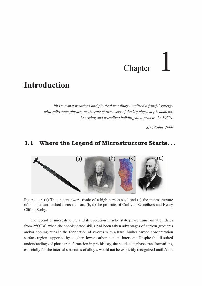
Figure 1.1: (a) The ancient sword made of a high-carbon steel and (c) the microstructure
of polished and etched meteoric iron. (b, d)The portraits of Carl von Schreibers and Henry
Clifton Sorby.
The legend of microstructure and its evolution in solid state phase transformation dates
from 2500BC when the sophisticated skills had been taken advantages of carbon gradients
and/or cooling rates in the fabrication of swords with a hard, higher carbon concentration
surface region supported by tougher, lower carbon content interiors. Despite the ill-suited
understandings of phase transformation in pre-history, the solid state phase transformations,
especially for the internal structures of alloys, would not be explicitly recognized until Alois
2 CHAPTER 1. INTRODUCTION
von Widmansten and Carl von Schreibers invented then-advanced metallography to reveal
the distinctive microstructure of polished and etched meteoric iron to the naked eyes in 1808
and Henry Clifton Sorby lifted the veil on metallic microstructure of a carburized Swedish
iron by using a reflected light microscopy in 1880 [PE12]. In the century to follow, the
perception of solid state phase transformation has been taking major steps forward accom-
panying with the invention and application of advanced characterization techniques to ex-
plore the interior microstructural features of steels. The utilization of optical microscopy
(OM) contributed to the identification of the pearlite, which opened the door to explore
the world of microstructure. The drawing of iron-base phase diagrams and the identifica-
tion of phase transformation temperature cannot be achieved without the thermal analysis.
The application of X-ray diffraction (XRD) to steels more than revealed an indisputable
fact that steels and other alloys are crystalline materials packed with atoms and defects,
but ushered in the research upsurge for martensitic transformation(MT) and other displacive
transformations. The advances in transmission electronic microscopy (TEM) allowed the
twinned microstructure of martensite and the relevant interfaces to be examined in great
detail. The advent of atom probe provided deeper insights into composition partitioning
during the phase transformations involving diffusion, like austenite decomposition, bainite
transformation, intermetallic precipitation, tempering, spinodal decomposition, etc. The em-
ployment of advanced characterization techniques and the renewal of experimental data also
inspired new theories and approaches to explore the physical natures of microstructural de-
velopment and properties in perspective of solid-state physics. These laws of physics nowa-
days are widely followed by a number of alloys more than applicable to steels. For example,
the adoption of principle of least action to strain energy led to Phenomenological Theory of
Martensite Crystallography (PTMC) which hits a great success to explain habit planes and
orientation relationships in a wide variety of ferrous and non-ferrous alloy systems under-
going MT[BM54a, BM54b, MB54]. The power law of self-organized criticality helped to
identify the nucleation and growth as the fundamental processes with characteristic rates to
govern solid state phase transformation. Darken[Dar48] recast Fick’s continuum diffusion
flux equations in terms of the chemical potentials to account for the uphill diffusion rather
than concentrations. Hillert et al.[Hil07] developed the computational thermodynamics and
kinetics to tackle the problems of equilibrium phase diagram, phase instability, precipitate
morphology, sizescaling, and pattern selection in diffusion controlled transformations. The
developed thermodynamic models and the corresponding functions, which are competent to
predicate energetic competition between phases [KRC62, ADP66a, ADP66b, MD69], have
been generalized as the CALPHAD (Calculation of Phase Diagram) approach today. Cahn
and Hilliard proposed the chemically diffuse interface model[CH58, Cah59, CH59] to ex-
1.2. MARTENSITES AND MARTENSITIC TRANSFORMATION 3
plain the spinodal decomposition. The model prototyping the continuous transformations
was then generalized into phase-field approaches[Ell89, WBM92]. Therefore, the encounter
with solid state physics in the mid 20th century indeed boosted the advance of metallur-
gical solid state phase transformations in view of the precise physical notions which are
brought to understand microstructural features. At the turn of the century, the PTMC has
been reinterpreted in the language of continuum elasticity[Bha03]; the multicomponent dif-
fusion has been viewed in Onsagers non-equilibrium thermodynamics; the weak first-order
MT has been connected with Landau’s phenomenological theory of phase transitions and
crystal lattice dynamics[Kru92]. With the help of computers, these physical models, under-
standings and intuitions have been applied to materials system with more complexity during
solid-state phase transformation. However, the theoretical studies nowadays are not going
far away from the key words of thermodynamics, crystallography, defects, diffusion, nucle-
ation, and growth, but are mainly focused on the adjustment of the microstructure and thus
the tuning of the properties of materials.
1.2 Martensites and Martensitic Transformation
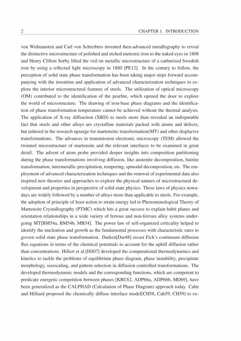
Figure 1.2: The portrait of Adolf Martens and the martensites in steel [Smi92] and shape
memory alloy [Chu93]
The terminologies of ’martensite’ and ’martensitic phase transformation’ were first used
in honor of Adolf Martens to identify the plate-like hard phase in a quenched carbon steel
[Nis12]. It is now common to find the term applied to structures in titanium alloys [GP00],
shape memory alloys(SMA) [OW99], ceramics [KR02] and other smart materials. The mor-
phology, crystal structures, nucleation modes, growth kinetics, and properties of various
martensites are divergent. The sole similarity that defines them as martensites is they are
formed via a shear-like diffusionless MT. According to Zhang [ZK09], the MT is one of
4 CHAPTER 1. INTRODUCTION
two categories of phase transformations in crystalline solids. (The other class is diffusional
transformation) MT has its distinctive characteristics as follows:
Among the most prominent is the simultaneous, cooperative movements of atoms over
distances less than an atomic diameter to product martensites as well as coherent or at least
approximating coherent interfaces paralleling with certain crystallographic planes. A co-
herent invariant plane is formed between a signal martensite plate and parent phase when
the constraint of invariant plane strain condition is satisfied. The habit plane is an abstract
crystallographic plane separating parent phase and aggregation of twin-related martensite
variants. Moreover, the mid-rib is also a kind of habit plane. The crystallographic lattice
correspondence exists between parent and martensite phases, which describes a relationship
between two involved lattices. It also allows the mechanism of atomic movements to explain
how each atom need move only a small fraction of an interatomic distance while as a whole
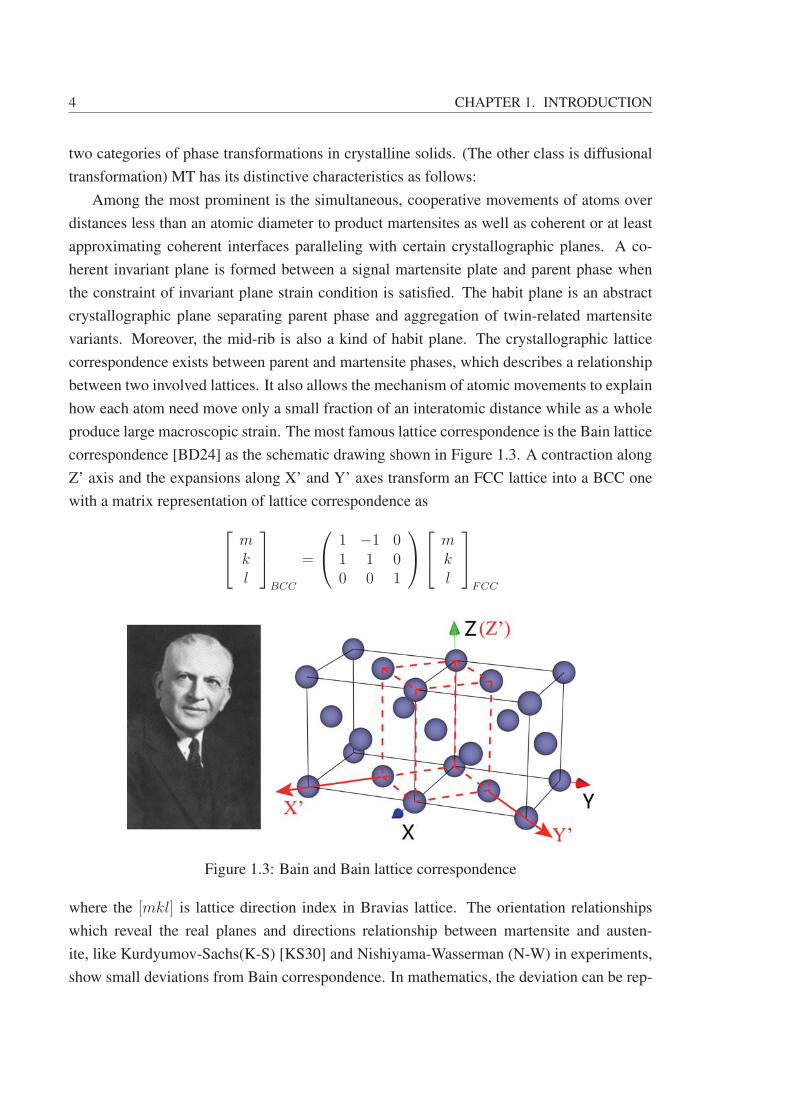
produce large macroscopic strain. The most famous lattice correspondence is the Bain lattice
correspondence [BD24] as the schematic drawing shown in Figure 1.3. A contraction along
Z’ axis and the expansions along X’ and Y’ axes transform an FCC lattice into a BCC one
with a matrix representation of lattice correspondence as
⎡⎣ m
kl
⎤⎦BCC
=
⎛⎝ 1 −1 0
1 1 00 0 1
⎞⎠⎡⎣ m
kl
⎤⎦
FCC
Figure 1.3: Bain and Bain lattice correspondence
where the [mkl] is lattice direction index in Bravias lattice. The orientation relationships
which reveal the real planes and directions relationship between martensite and austen-
ite, like Kurdyumov-Sachs(K-S) [KS30] and Nishiyama-Wasserman (N-W) in experiments,
show small deviations from Bain correspondence. In mathematics, the deviation can be rep-

1.2. MARTENSITES AND MARTENSITIC TRANSFORMATION 5
resented by a rigid body rotation. MT doesn’t involve long range diffusion, such that the
parent and product phases have no distinct compositional difference, although recent atom
probe tomographic analysis reveals that atomic relaxation and short range diffusion can take
place during MTs [TMH+14, TMR15].
In dynamics, MT proceeds at fast speed approaching the velocity of sound in the matrix
crystal, if nothing more than small ’shuffles’ or co-operative atom movements occurs during
MT. MT requires an undercooling to trigger the transformation, thus the onset temperature
of MT, i.e. Ms, is measured lower than the T0 temperature at which the parent phase and
martensite have the same Gibbs energy. The Ms varies with composition and mechanical
deformation but is scarcely influenced by the quenching processing. MT is usually ather-
mal, which means no thermal activation is necessary for the transformation to proceed. The
amount of generated martensite is not linearly related to temperature fall between the Ms and
Mf (at which the MT halts). Actually, the athermal MT can occur in most of systems, even
for those of particular steels and copper alloys which have ability to introduce an isothemal
MT at a constant temperature.
The thermoelasticity is another generic feature of MT in SMAs and gives rise to the
temperature hysteresis and shape memory effect. The different behaviors of hysteresis in
SMAs are more than relevant to the eigen transformation strains but also affected by the
dislocation creation and the friction of the interfaces. The irreversibility of MT in carbon
and low alloy steels are related to other diffusional transformations in competition with MT.
At As temperature (at which reversion to austenite occurs on heating) of carbon steel, the
decomposition of martensite to carbides and ferrite occurs before the austenite can reform
due to the fast diffusion of carbon.
Based on the reviewing, none of the above characteristics can be acted as the sufficient
and necessary criterion to define a transformation as MT or not. For example, the surface
relief was discovered in γ − AlAg2 phase [LA69] after a phase transformation involving
composition changes. The burgers orientation relationship was identified in β − α transfor-
mation in titanium alloys. The existence of aforementioned counterexamples leads to a long
term controversy and challenge in the definition of MT. The precise definition of the MT
becomes increasing difficult as the accumulation of evidences and theoretical reconsidera-
tions. In a narrow sense [HSU80], the MT is a first-order phase transformation undergoing
nucleation and growth through diffusionless atomic displacement, either uniform or non-
uniform.It leads to particular microstructural features such as shape change, surface relief
and satisfaction of invariant plane strain condition. In contrast, the general definition of MT
in accordance with Khachaturyan [Kha13] is depicted as ’a phase transformation that can
be treated in terms of displacement only is called a MT’. The significant difference between
6 CHAPTER 1. INTRODUCTION
two definitions is that the latter takes the improper MT into consideration, such that a MT
not necessarily is a classical first-order transformation undergoing a nucleation and growth
process. It is because the threshold for first-order and high-order displacive transformations
and the dividing line of nucleation and growth in some weak MTs are no longer clear in
perspective of the crystal lattice dynamics. In an extreme case, a transformation triggered by
the shuffle that generates a zero deformation strain without any macroscopic shape change
can also be recognized as a MT. However, most of the improper MTs exhibit transformation
strains, which are always treated as the secondary order parameters(OPs) in modern Lan-
dau theory of phase transformation. Moreover, invariant plane condition is not necessary
either to define a MT. The MT can be only with the dilatational deformation. In this thesis,
we accept the general definition of the MT by Khachaturyan, which is in accordance with
nonlinear nonlocal Landau theory of the phase transformation.
1.3 Motivations
From the definition of MT, we understand that the MT is a relative complex transforma-
tion sensitive to chemical, thermal and mechanical conditions and also competes with other
diffusional transformations. Therefore, various theories and models have been developed
to understand the physical natures of the MT in different perspectives. The most important
theories include: the PTMC to account for the microstructural features based on kinematiccompatibility, the microelasticity phase-field model to present the intriguing microstructure
of martensites based on Green’s function in continuum mechanics of elasticity and Allen-Cahn equation in statistical mechanics, Landau theory to focus on the dynamical behaviors
with the wisdom of crystal lattice dynamics and hydrodynamics, etc., which are all intro-
duced in the following chapters. Although differing in statics and/or dynamics due to their
individual origins in branches of physics, these theories must share certain common ingredi-
ents with each other and exhibit distinctive advantages. However, the physical connections
and distinctions among the theories/models have not been addressed yet. A deeper under-
standing of the theories with a unified perspective of physics benefits to building a panorama
of phase transformations and enables us to select the most appropriate theory for a real prob-
lem, which is the first motivation of the thesis.
Moreover, the investigation of martensite and the relevant phase transformations are far
from complete with the current theories and models: Martensitic nucleation is one of out-
standing challenges. In experiments, an accurate measurement of absolute interfacial en-
ergies remains the biggest source of uncertainty [LEA89], not to mention the continuing
inability to directly observe nucleation at the atomic scale. Another challenge is that the

1.4. OUTLINE OF THE THESIS 7
complexity of real microstructures, as the consequence of the interplaying of different fields
including strains, compositions, dislocations, grain boundaries in multiscales, still eludes the
rigorous quantitative description and control of microstructure to satisfy the requirement of
industry. Therefore, the second motivation of the thesis is to put forward a prototype model
that couples various fields of transformation strain, diffusion potential, grain orientations,
and dislocation density to simulate the nucleation and growth of martensites under more
complex conditions.
1.4 Outline of the Thesis
The thesis is organized into three sections. The first section in chapter 2 details the
current state-of-the-art models for exploring the microstructural features and the mechani-
cal behaviors of martensites. They are the Phenomenological Theory of Martensite Crys-
tallography (PTMC) as well as its reinterpretation within the framework of the continuum
mechanics (CM-PTMC), Khachaturyans microelasticity phase field method, and the Landau
theory based on the Irreducible Representation of the point groups and transformation Strains
(IRS). The similarities and differences among these theories/models are detailed by means
of theoretical analyses and/or simulations for two-dimensional square-to-rectangle as well
as three-dimensional cubic-to-tetragonal and cubic-to-trigonal martensitic transformations.
The second section, which encompasses chapters 3 and 4, presents a novel nonlinear dy-
namic Landau model and its application to describe the first-order MTs in polycrystalline
ferroelastic materials. The mathematical description is developed in chapter 3, where the
construction of Landau energy and numerical solution scheme are presented in detail. Sim-
ulations of 2D polycrystalline square-to-rectangle and triangle-to-centered rectangle MTs
are used to validate our model and demonstrate the physical consistence of the model with
CM-PTMC. In chapter 4, the nonlinear dynamic Landau model is applied to study dynamical
nucleation in MTs. It shows how the quenching temperature, the applied stress and the intrin-
sic transformation energy can be combined to activate particular mechanisms of martensitic
nucleation and growth in polycrystals.
The third section of the thesis in chapters 5-6 is devoted to further developing the Landau
model, which is integrated with models that take into account diffusional transformations
and the effect of dislocations. The development of the model for diffusive-displacive cou-
pled phase transformations is presented in chapter 5. In this approach, the Landau model
is coupled with the information provided by thermo-kinetic calculation and databases to ob-
tain the material parameters that control the diffusion potential and the quantitative mobility
during diffusive transformations. As an example of application, this coupled model is used

8 CHAPTER 1. INTRODUCTION
to study the carbon redistribution in steels manufactured by the quenching and partitioning
(Q&P) process. In chapter 6, a modified continuum dislocation model is proposed and seam-
lessly embedded into the coupled Landau model introduced in chapter 5. This model is used
to analyze the interplay among dislocations, driving forces for martensitic transformations
and diffusion on the microstructure evolution of steels.
Finally, the conclusions and the avenues for future work within the framework of inte-
grated computational materials engineering are briefly summarized in Chapter 7.
Chapter 2Models of Martensitic Transformation
A method is more important than a discovery, since the right method will lead to new.
-Lev Landau
This chapter reviews the various current models of MT from viewpoints of geometry,
elasticity, wave mechanics and their integration. The intrinsic connections and distinctions
in physics are comprehensively discussed via theoretical analysis and the comparison of
simulation results. It serves as the fundamental task to develop novel integrated models for
the coupled phase transformation.
2.1 Preliminaries of Continuum Mechanics
According to Khachaturyan’s general definition [Kha13], MT is one category of phase
transformations which could be only described in terms of displacements. Therefore, mod-
eling of MT can be started with the definition of the austenite and martensite lattices in mean
of vector algebra, followed by the description of lattices and symmetries changes during the
MT [Bha03]. Mathematically, a perfect crystal can be abstracted as a point lattice, gener-
ated by periodically stacking of unit cell in 3D space. An arbitrary lattice position can be
expressed as fractions or multiples of unit-cell dimensions, or in a viewpoint of continuum
mechanics, as a vector of
v = a1e1 + a2e2 + a3e3 (2.1)
linking origin and lattice position in a reference coordinate system, where {ai} is the pro-
jected length of the vector {ei} along each of the three independent unit axes. The descrip-
tion of lattice in atomic lattice scale is actually a particular case in continuum scale when the
10 CHAPTER 2. MODELS OF MARTENSITIC TRANSFORMATION
edges of unit cell are chosen as the reference coordinate system. The lattice-continuum con-
nection is revealed by Cauchy-Born hypothesis [Zan96], which will be detailed later. Based
on this connection, the concepts of deformation and displacement in an elastic continuum
are introduced into MT, such that a MT can be described as a deformation linking austenite
and martensite. Provided that any material point at position x in non-deformed austenite
moves to a new position y(x) in deformed martensite, the martensitic configuration, or the
deformation itself, is expressed as
y (x) = x+ u (x) (2.2)
where u(x) is displacement of any material point. The deformation gradient F is defined
as the partial derivatives of the deformation y with respect to space coordinates x; then the
matrix of deformation gradient reads
F = ∇y,
Fij =∂yj∂xi
, (i, j = 1, 2, 3)(2.3)
With a deformation gradient, most of the variables in continuum elasticity can be readily
expressed. Expanding the displacement term in the full differentiation form of Eq(2.2)
dy (x) = dx + du (x) into the Taylor series, and dropping the second and higher terms
leads to
dy (x) = dx+∂u (x)
∂xdx = (I+∇u) dx. (2.4)
where I is the identity matrix. Thus, deformation gradient is connected with displacement
gradient by
F = I+∇u (x) (2.5)
The full differentiation form
dy = F (x0) dx (2.6)
also describes that an infinitesimal line element dx at given point x0 goes to the element dy
after deformation.
In addition, strain in any given direction ei can be defined as the ratio of the local defor-
mation to initial length
ε =|dy| − |dx|
|dx| =
√dy · dy|dx| − 1 (2.7)
Applying full differentiation Eq.(2.6) gives rise to
ε =
√Fdx · Fdx|dx| − 1 =
√F
dx
|dx| · Fdx
|dx| − 1
=√Fe · Fe− 1 =
√e · (FTFe)− 1
(2.8)
2.1. PRELIMINARIES OF CONTINUUM MECHANICS 11
such that the finite strain tensor written in deformation gradient is
ε =1
2
(FTF− I
)=
1
2(C− I) (2.9)
where C = FTF is Cauchy-Green deformation tensor, and FT is the transpose of deforma-
tion gradient F. Inserting Eq. (2.5) into Eq.(2.9), we obtain the finite strain tensor written in
displacement gradient, with the strain component
εij =1
2
(∂ui
∂xj
+∂uj
∂xi
+∑k
∂uk
∂xi
∂uk
∂xj
)(2.10)
Neglecting the non-linear term, the infinitesimal strain is
ε =1
2
[(∇u) + (∇u)T
], εij =
1
2
(∂ui
∂xj
+∂uj
∂xi
)(2.11)
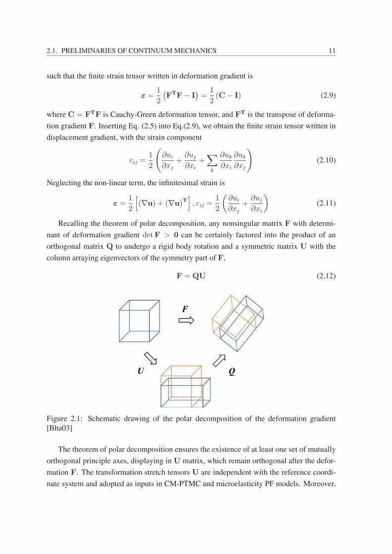
Recalling the theorem of polar decomposition, any nonsingular matrix F with determi-
nant of deformation gradient detF > 0 can be certainly factored into the product of an
orthogonal matrix Q to undergo a rigid body rotation and a symmetric matrix U with the
column arraying eigenvectors of the symmetry part of F,
F = QU (2.12)
Figure 2.1: Schematic drawing of the polar decomposition of the deformation gradient
[Bha03]
The theorem of polar decomposition ensures the existence of at least one set of mutually
orthogonal principle axes, displaying in U matrix, which remain orthogonal after the defor-
mation F. The transformation stretch tensors U are independent with the reference coordi-
nate system and adopted as inputs in CM-PTMC and microelasticity PF models. Moreover,

12 CHAPTER 2. MODELS OF MARTENSITIC TRANSFORMATION
the eigenvalues corresponding to the eigenvectors are determined by solving |C− λ2I| = 0
or in a bilinear form
FTF = λ21e
eig1 ⊗ eeig1 + λ2
2eeig2 ⊗ eeig2 + λ2
3eeig3 ⊗ eeig3 (2.13)
Besides the deformation of a line element, Figure 2.2 illustrates the deformation of vol-
ume and area elements. Considering a parallelepiped material volume spanned by three inde-
pendent vectors a = a1e1+a2e2+a3e3,b = b1e1+b2e2+b3e3, and c = c1e1+c2e2+c3e3 in
the reference, the volume is expressed as the absolute value of scalar triple product (a× b)·c,
which can be reformulated as
V =
∣∣∣∣∣∣det⎡⎣ c1 c2 c3
a1 a2 a3b1 b2 b3
⎤⎦∣∣∣∣∣∣ (2.14)
Using the definition of deformation gradient, a differential material volume dv with local
volume change is connected to non-deformed configuration dV by the determinant of defor-
mation gradient,
dv = (detF) dV (2.15)
Analogically, if a material area A (expressed in vector An = x× z with unit normal n)
is transformed into the area a (am = x′ × z′ with unit normal m) after deformation, and
the edge vectors are deformed via the deformation gradients as x′ = Fx and z′ = Fz, the
deformed area can be connected with non-deformed area by
da = |(cofF)n| dA, m =F−Tn
|F−Tn| (2.16)
where cofF = (detF)F−T is cofactor of F.
It should be note that the deformation depicted by all of models in the thesis is such a
deformation where neither a finite volume (a point) is compressed (expanded) to a point (a
finite volume), nor the body penetrates itself. Thus, it ensures a satisfaction of the condition
detF > 0. As the right-hand sets of coordinates are appointed in the thesis, the positive
determinant condition is equivalent to that the triple product of unit vectors before and after
transformation must have the same sign, viz. e1 · (e2 × e3) > 0.
2.2 Prototype Phenomenological Theory of Marten-site Crystallography (PTMC)
The prototype PTMC theory were developed independently by Wechsler et al. (WLR)
[WRL60, Lie58, Wec59, LRW57] and Bowles and Mackenzie (BM) [BM54a, BM54b, MB54]
2.2. PROTOTYPE PHENOMENOLOGICAL THEORY OF MARTENSITE
CRYSTALLOGRAPHY (PTMC) 13
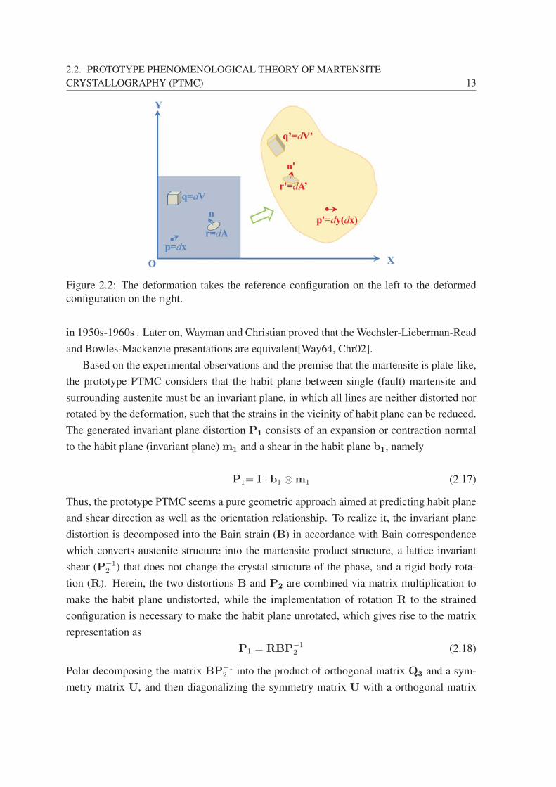
Figure 2.2: The deformation takes the reference configuration on the left to the deformed
configuration on the right.
in 1950s-1960s . Later on, Wayman and Christian proved that the Wechsler-Lieberman-Read
and Bowles-Mackenzie presentations are equivalent[Way64, Chr02].
Based on the experimental observations and the premise that the martensite is plate-like,
the prototype PTMC considers that the habit plane between single (fault) martensite and
surrounding austenite must be an invariant plane, in which all lines are neither distorted nor
rotated by the deformation, such that the strains in the vicinity of habit plane can be reduced.
The generated invariant plane distortion P1 consists of an expansion or contraction normal
to the habit plane (invariant plane) m1 and a shear in the habit plane b1, namely
P1= I+b1 ⊗m1 (2.17)
Thus, the prototype PTMC seems a pure geometric approach aimed at predicting habit plane
and shear direction as well as the orientation relationship. To realize it, the invariant plane
distortion is decomposed into the Bain strain (B) in accordance with Bain correspondence
which converts austenite structure into the martensite product structure, a lattice invariant
shear (P−12 ) that does not change the crystal structure of the phase, and a rigid body rota-
tion (R). Herein, the two distortions B and P2 are combined via matrix multiplication to
make the habit plane undistorted, while the implementation of rotation R to the strained
configuration is necessary to make the habit plane unrotated, which gives rise to the matrix
representation as
P1 = RBP−12 (2.18)
Polar decomposing the matrix BP−12 into the product of orthogonal matrix Q3 and a sym-
metry matrix U, and then diagonalizing the symmetry matrix U with a orthogonal matrix
14 CHAPTER 2. MODELS OF MARTENSITIC TRANSFORMATION
Q4, the invariant plane distortion P1 is reformulated as
P1 = RQ3Q4UdQT4 (2.19)
where Ud =
⎡⎣ λ1
λ2
λ3
⎤⎦ is a diagonal matrix describing the transformation stretch in
principal space. Thus, we obtain the identical relationship PT1P1=Q4U
2dQ
T4 , which indi-
cates that PT1P1 and U2
d have same eigenvalues and the eigenvectors of PT1P1 can be linked
to the orthogonal basis of U2d by a pure rotation. In geometry, it means that any vector v in
habit plane remains unchanged in magnitude, and the property can be depicted in austenite
coordinates vTv = vTP−T2 BTBP−1
2 v or in principal space vTdU
2dvd= vT
dvd. In this way,
the task of solving b and m thoroughly comes down to an eigenvalue-eigenvector problem.
2.2.1 Wechsler-Lieberman-Read Method
Starting with a predefined lattice invariant shear P−12 written in principal bases expanded
by eigenvectors of U2d, the shear takes the form of simple shear
< Cd
∣∣P−12
∣∣Cd >=
⎡⎣ 1 g
11
⎤⎦ (2.20)
here, the Dirac notation is used to specify the coordinates where the vector or tensor spans.
|Cd >,|Cfcc >, and |Cbcc > are bases to describe the space coordinates of principal space,
austenite and martensite, respectively. The principal bases can be transformed to the bases
of austenite via a rotation Q5. The Q5 has the column vectors of unit shear direction
of invariant plane b2, unit direction of shear plane normal m2, and a third vector given
by the vector product v2 = b2 × m2 expressed in austenite coordinates, viz. Q5 =
(b2,m2,v2). Therefore, we rewrite the Bain strain (distortion) in principal space by <
Cd |B|Cd >=< Cd
∣∣QT5
∣∣Cfcc >< Cfcc |B|Cfcc >< Cfcc |Q5|Cd >, and the total dis-
tortion in principal space is < Cd |B|Cd >< Cd
∣∣P−12
∣∣Cd >. Solving the characteristic
equation∣∣P−T
2 BTBP−12 − λ2I
∣∣ = 0 and inserting λ22 = 1, we can get two sets of eigen-
values of (λ21, λ
23) associated with two values of g in Eq.(2.20) as well as the eigenvectors.
Representing these eigenvectors in austenite coordinates by means of rotation matrix Q5 and
utilizing the bilinear form PT1P1=Q4U
TdUdQ
T4= P−T
2 BTBP−12 , the orthogonal matrix Q4
and BP−12 are determined. Now admitting an invariant line vector in the habit plane defined
by vTdU
2dvd= vT
dvd, the trial solutions of vd are used to determine the possible habit plane
normal m1 and invariant plane deformation b1. Using the Eqs.(2.17) and (2.19), the rotation
R can be solved.
2.2. PROTOTYPE PHENOMENOLOGICAL THEORY OF MARTENSITE
CRYSTALLOGRAPHY (PTMC) 15
2.2.2 Bowles-Mackenzie Method
In practice, there is little difference in calculation procedures between Bowles-Mackenzie
and Wechsler-Lieberman-Read methods. The implementation of Bowles-Mackenzie method
firstly introduces the concept of invariant line defined as the vector of intersection of the two
invariant planes m1 and m2, which is unaltered in both magnitude and direction during
two distortions. Correspondingly, an invariant line distortion S is defined as the resultant of
invariant plane distortion P1 and P2,
P1P2= S = RB (2.21)
With a predefined lattice invariant shear P2 and an established invariant line distortion S
written in the coordinates of austenite, an elaborate analysis in geometry results in the ex-
pression of shear direction
b1=Sb2−b2
m1 · b2
(2.22)
and the habit plane normal m1 is related to the normal of invariant plane shear m2 as
m1 ‖ S−Tm2 −m2 (2.23)
Therefore, determination of invariant line distortion S is the key issue in BM method. Oppo-
site to WLR method solving eigenvalues in principal space and then transforming to austen-
ite coordinates, the BM method firstly obtains the invariant lines x and invariant normals by
solving a set of ellipsoid equations describing the direction and plane normal on unextended
cones along with the predefined lattice invariant shear P2 in austenite coordinates. Similar
to WLR, the obtained invariant line x, plane normal of lattice shear m2, and a third vector
given by the vector product v1 = x × m2 are served as the column vectors of a rotation
R1 = (x,m2,v1), which represent the orthogonal bases < Cinv |I > in the coordinates of
austenite. Analogously, another orthogonal bases will be defined as R2 = (x¯,m
¯ 2,v2) by
using the position of the invariant line after the Bain distortion x¯, unit vector parallel to the
final position of the normal m¯ 2,and v2 = x
¯× m
¯ 2. In a specific way, we have
x¯=< Cfcc |B|Cfcc >< Cfcc |x > (2.24)
m¯ 2 =
< Cfcc |B|Cfcc>−1 < Cfcc |m2 >
(< m2 |Cfcc >< Cfcc |B|Cfcc>−2 < Cfcc |m2 >)1/2(2.25)

16 CHAPTER 2. MODELS OF MARTENSITIC TRANSFORMATION
It is easy to find that there is a distortion Sp=R1RT2B that leaves the invariant line x and
shear plane normal m2 unextended. Representing the pure shear distortion Sp in principle
space by similarity transformation, we have
< Cd |Sp|Cd >=< Cd
∣∣RT1
∣∣Cfcc >< Cfcc |R1|Cd >< Cd
∣∣RT2
∣∣Cfcc >< Cfcc |B|Cfcc >< Cfcc |R1|Cd >=< Cd
∣∣RT2
∣∣Cfcc >< Cfcc |B|Cfcc >< Cfcc |R1|Cd >(2.26)
The most general invariant line distortion in principal space only requires rotating the invari-
ant line by R to make itself unextended and unrotated.
< Cd |S|Cd >=< Cd |R|Cd >< Cd
∣∣RT2
∣∣Cfcc >< Cfcc |B|Cfcc >< Cfcc |R1|Cd >
(2.27)
where the rotation < Cd |R|Cd > in principal axes is expressed as
< Cd |R|Cd >=
⎡⎣ 1
cos β − sin βsin β cos β
⎤⎦ (2.28)
By solving the equation of invariant normal < Cd |S|Cd >< Cd |n > =< Cd |n > ,
the rotation matrices < Cd |R|Cd > and < Cd |S|Cd > are uniquely calculated, and the
invariant line distortion S in austenite coordinates can be completely determined by mean of
similarity transformation,
< Cfcc |S|Cfcc >=< Cfcc |R1|Cd >< Cd |S|Cd >< Cd
∣∣RT1
∣∣Cfcc > (2.29)
Substituting Eq.(2.29) into Eqs.(2.22) and (2.23), the invariant plane normal and shear can
be solved.
2.3 Continuum Mechanical Reinterpretation ofPTMC (CM-PTMC)
The prototype PTMC theories in pure geometry have been further developed by Ericksen
[Eri85, Eri05], Ball and James [BJ89, Bal02, Bal04], and Bhattacharya et al. [Bha03] They
utilized the Cauchy-Born hypothesis to describe the invariance of properties, including the
invariance of geometry and Hamiltonian under certain crystallographic symmetry operation.
Rendering elasticity theory flexible enough by incorporating the perspectives of group theory
2.3. CONTINUUM MECHANICAL REINTERPRETATION OF PTMC (CM-PTMC) 17
and implementing the variation, the linear/nonlinear elastic models of MT in crystals were
developed. It also laid foundations for long outside its range of elasticity, leading to an
increasing bulk of achievements, especially aimed at the understanding and prediction of
microstructure formation during MTs. With the elastic model, the microstructural features
of martensites and their orientation relationship with parent austenite can be solved by the
minimization of energy with respect to the constraint of kinematic compatibility, all of which
are consolidated in Bhattacharya’s prestigious textbook [Bha03].
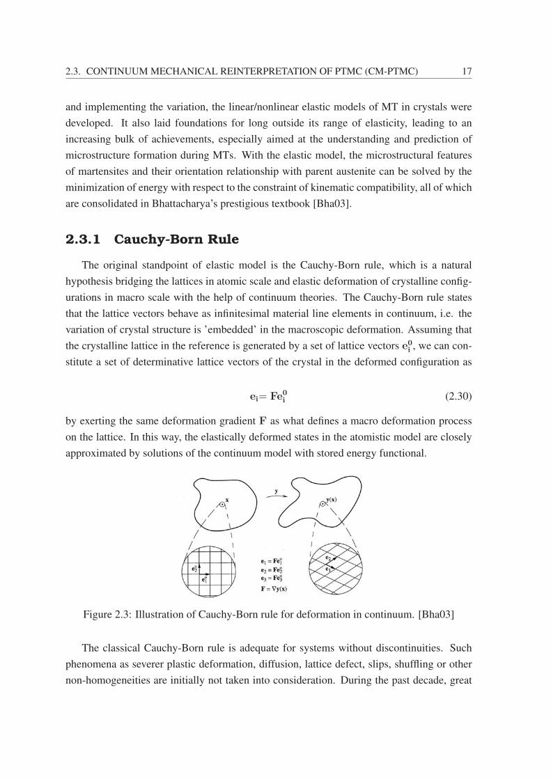
2.3.1 Cauchy-Born Rule
The original standpoint of elastic model is the Cauchy-Born rule, which is a natural
hypothesis bridging the lattices in atomic scale and elastic deformation of crystalline config-
urations in macro scale with the help of continuum theories. The Cauchy-Born rule states
that the lattice vectors behave as infinitesimal material line elements in continuum, i.e. the
variation of crystal structure is ’embedded’ in the macroscopic deformation. Assuming that
the crystalline lattice in the reference is generated by a set of lattice vectors e0i , we can con-
stitute a set of determinative lattice vectors of the crystal in the deformed configuration as
ei= Fe0i (2.30)
by exerting the same deformation gradient F as what defines a macro deformation process
on the lattice. In this way, the elastically deformed states in the atomistic model are closely
approximated by solutions of the continuum model with stored energy functional.
Figure 2.3: Illustration of Cauchy-Born rule for deformation in continuum. [Bha03]
The classical Cauchy-Born rule is adequate for systems without discontinuities. Such
phenomena as severer plastic deformation, diffusion, lattice defect, slips, shuffling or other
non-homogeneities are initially not taken into consideration. During the past decade, great
18 CHAPTER 2. MODELS OF MARTENSITIC TRANSFORMATION
efforts have also been devoted to the development of integrated models incorporating dislo-
cation and plasticity, which will be detailed in chapters 5 and 6. Anyway, the Cauchy-Born
rule and the elastic model can be safely applied to MTs in SMAs and other materials whose
crystalline structure is given by a simple Bravais lattice.
2.3.2 Frame Indifference and Materials Symmetry
Distinct from the pure geometric prototype PTMC, the CM-PTMC considers geomet-
ric and energetic invariance under symmetry operations of crystals. In CM-PTMC, we as-
sume that the energy density stored in a crystalline lattice depends on the lattice vectors and
temperature and satisfies frame-indifference and constraint of materials symmetry, which
coincide with Landau theory for the second order phase transitions. The property of frame-
indifference signifies that the energy density ϕ is observed in an inertial reference system,
and a rigid body rotation of the lattice or a change of observer will not change the energy
itself, i.e.
ϕ (ei, T ) = ϕ (Qei, T ) (2.31)
If the same reference coordinates are chosen for both lattices configurations before and
after transformation, and the Cauchy-Born rule is utilized, the lattice based energy density
can be reformulated as a continuum energy density with independent variable of deformation
gradient. The frame-indifference property expressed in continuum energy density follows
ϕ (F, T ) = ϕ (QF, T ) (2.32)
It can be seen that, the CM-PTMC has advantage to describe the deformation gradient in
an independently defined coordinates, avoiding the error-prone transformations between the
principal space where eigenvalues and eigenvectors are explicitly revealed and the laboratory
coordinates where the materials actually exist.
The materials symmetry indicates that the properties of a crystalline solid, including
energy density and its derivatives, are identical in crystallographic equivalent directions. In
other words, exerting same deformation on two identical materials from two crystallographic
equivalent directions gives rise to the same energy density. In mathematics, the property of
materials symmetry reads
ϕ (FR, T ) = ϕ (F, T ) for all rotations R ∈ P (e◦i ) (2.33)
or conventionally
ϕ(RTFR, T
)= ϕ (F, T ) for all rotations R ∈ P (e◦i ) (2.34)
2.3. CONTINUUM MECHANICAL REINTERPRETATION OF PTMC (CM-PTMC) 19
where P (e◦i ) is the point group of a lattice.
It is obvious that the similarity transformation by an orthogonal matrix of pure rotation
does not alter the eigenvalues of deformation gradient. For this reason, the development of
the (meta) stable microstructure in MT is simplified as the representation of the piecewise
deformation gradients lying in austenite and/or martensite variants. In the thesis, we confine
the symmetry operations in point group P (e◦i ) instead of symmetry groups of lattice, because
we limit the deformation associated with MT is small compared to the lattice.
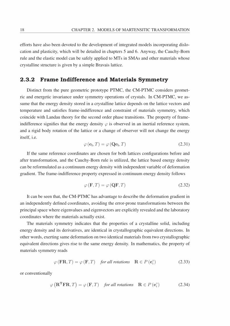
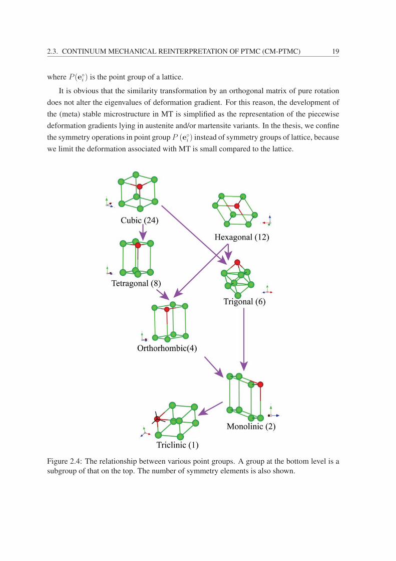
Figure 2.4: The relationship between various point groups. A group at the bottom level is a
subgroup of that on the top. The number of symmetry elements is also shown.
20 CHAPTER 2. MODELS OF MARTENSITIC TRANSFORMATION
2.3.3 Martensite Variants
Antecedent to the Landau’s theory of phase transformations, the group theory had been
served as a powerful tool to study structural transformation. The core argument of the group
based construction of structural transformation indicates that the deformation variants are
subjected to constraints of transformation path degeneracy and the symmetry of Hamiltonian.
With the wisdom of group theory blended in, the MT in CM-PTMC is modeled by the free
energy with multiply energy wells for parent phase and martensite variants. The martensite
variants are provided with characteristic transformation strains and identical energy density
associated with iso-energetic wells on energy surface. If only the invariant rotations are
considered, the martensite variants can be transformed into each other by implementing any
symmetry operation belonging to the point group. And the number of deformation variants
can be determined by calculating the symmetry operations lost in the martensitic lattice in
comparison with those in parent phase. [Bha03].
nv =n [PAustenite (e
◦i )]
n [PMartensite (e◦i )](2.35)
It is noteworthy that we confine the proper rotational operations in group and subgroups
hereinafter. The other invariant operations, such as reflections, translations and their combi-
nation, constituting the lattice group are ignored. Thus, the slip martensite variants associated
with the orientation relationship are not taken into consideration in this thesis. For the details
of two different transformation paths of degeneracy can be referenced in [Gao13].
2.3.4 St.-Venant’s Compatibility and Kinematic Compati-bility
Recalling the prototype PTMC, it is understood that the deformation gradient not only
describes the continuum elastic energy density at a specific temperature, but also determines
the microstructure features. A MT to form a coherent interface requires a continuous, single-
valued displacement or deformation field to indicate that the material is unbroken. The con-
tinuous field constraint, named St.-Venant’s compatibility, refers as the curl of deformation
gradient vanishes everywhere in mathematics.
∇× F = 0 (2.36)
which is of significance in the following chapters relevant to long-range elastic compatibility
kernel in IRS description of martensites (in chapters 3-4) and the MT coupled with dislo-
cation (Chapter 6). Besides the continuous displacement field, the formation of coherent
2.3. CONTINUUM MECHANICAL REINTERPRETATION OF PTMC (CM-PTMC) 21
interface also requires the satisfaction of the ’invariant plane condition’. Although the defor-
mation gradients are not required continuous to describe an invariant plane, they can not be
arbitrary matrices across the interface, and must satisfy kinematic compatibility condition in
CM-PTMC, which is the generalized form of invariant plane condition [Bha91, BC99] .
F = I+ b⊗mFj − Fi = a⊗ n
(2.37)
where Fi is the deformation gradient matrix, m and n are the plane normals; a and b are the
shear vectors. ⊗ designates dyadic product and I is the identity matrix. If an arbitrary vector
v is considered lying on the interface, we have
Fiv − Fjv = (a⊗ n) · v = a (v · n) = 0 (2.38)
The kinematic compatibility condition is proven equivalent to invariant plane condition
in prototype PTMC. Hereafter in the thesis, we no longer distinguish the ’lattice invariant
shear’ (P2) condition and ’invariant plane distortion’ (P1) condition to form habit plane, but
utilize the kinematic compatibility equation in Eq.(2.37).
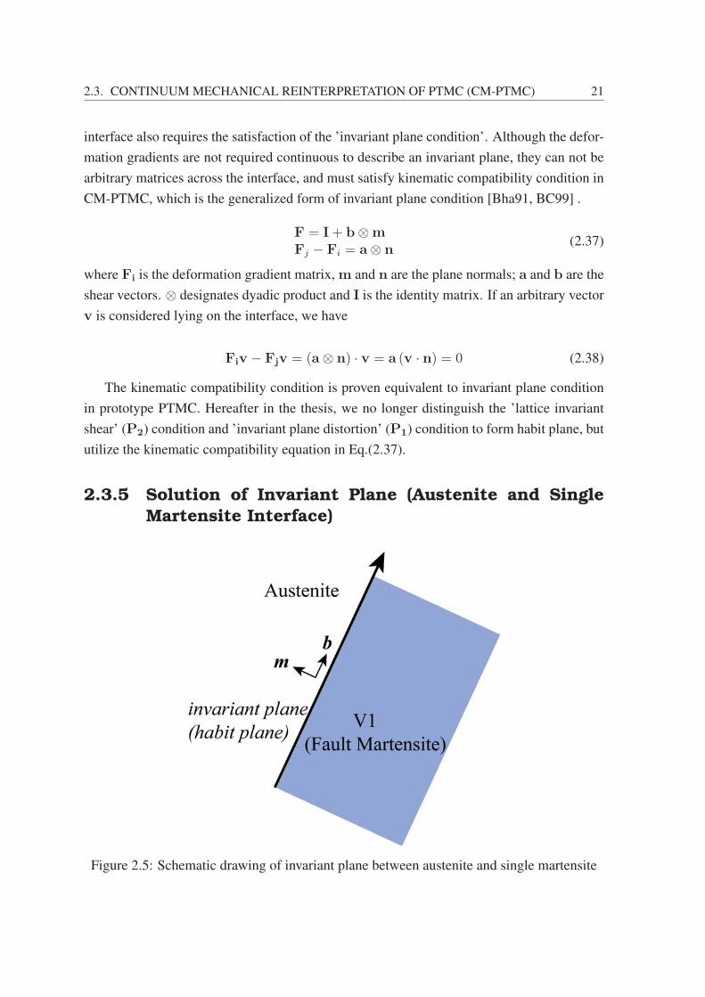
2.3.5 Solution of Invariant Plane (Austenite and SingleMartensite Interface)
Figure 2.5: Schematic drawing of invariant plane between austenite and single martensite
22 CHAPTER 2. MODELS OF MARTENSITIC TRANSFORMATION
For the interface of single martensite and austenite, the deformation gradients on both
sides of the interface are
∇y(x)
{I (x ∈ A)
F = QUi (x ∈ M)(2.39)
Considering the kinematic compatibility condition in Eq.(2.37), we have Cauchy-Green de-
formation tensor
C =FTF =(I+ b⊗m)T (I+ b⊗m)= (I+m⊗ b) (I+ b⊗m)= I+ b⊗m+m⊗ b+ (m⊗ b) (m⊗ b)= I+ b⊗m+m⊗ b+mi (bkbk)mj
= I+ b⊗m+m⊗ b+b · b2
m⊗m+m⊗ b · b2
m
(2.40)
= I+
(b+
b · b2
m
)⊗m+m⊗
(b+
b · b2
m
)Recalling Eq.(2.13) and subtracting an identity matrix on the both sides of the equation, we
have
FTF− I =(λ21 − 1
)eeig1 ⊗ eeig1 +
(λ22 − 1
)eeig2 ⊗ eeig2 +
(λ23 − 1
)eeig3 ⊗ eeig3 (2.41)
To make the form of Cauchy-Green tensor satisfying both Eqs.(2.40) and (2.41), one of the
eigenvalues of Cauchy-Green tensor should be less than 1, the second one must be equal to
1 and the remaining one is larger than 1. Provided that
λ21 < 1, λ2
2 = 1, λ23 > 1 (2.42)
there are two sets of solutions for invariant plane normal and shear direction⎧⎪⎪⎪⎪⎨⎪⎪⎪⎪⎩
m1 =
√λ23 − 1
λ23 − λ2
1
eeig3 +
√1− λ2
1
λ23 − λ2
1
eeig1
¯b1 =1
2(λ2
3 − λ21)
(√λ23 − 1
λ23 − λ2
1
eeig3 −√
1− λ21
λ23 − λ2
1
eeig1
) (2.43)
⎧⎪⎪⎪⎪⎨⎪⎪⎪⎪⎩
m2 =
√λ23 − 1
λ23 − λ2
1
eeig3 −√
1− λ21
λ23 − λ2
1
eeig1
¯b2 =1
2(λ2
3 − λ21)
(√λ23 − 1
λ23 − λ2
1
eeig3 +
√1− λ2
1
λ23 − λ2
1
eeig1
) (2.44)
Substituting the solution of ¯b and m into ¯b = b+b · b2
m leads to the solutions of b,
b1 =1
2(λ3 − λ1)
(λ1
√λ23 − 1
λ23 − λ2
1
eeig3 − λ3
√1− λ2
1
λ23 − λ2
1
eeig1
)(2.45)

2.3. CONTINUUM MECHANICAL REINTERPRETATION OF PTMC (CM-PTMC) 23
b2 =1
2(λ3 − λ1)
(λ1
√λ23 − 1
λ23 − λ2
1
eeig3 + λ3
√1− λ2
1
λ23 − λ2
1
eeig1
)(2.46)
Here, we utilize the Cauchy-Green tensor instead of deformation gradient F to solve the
eigenvalues and eigenvectors. In other words, any contribution from rotation is eliminated
due to QTQ = I. The calculated invariant plane normal and shear are exclusively deter-
mined by the reference independent transformation stretch U. Thus in practice, the inspec-
tion of kinematic compatibility condition for a specific material in laboratory should allow
an additional degree of freedom of a rigid-body rotation.
2.3.6 Solution of Twin Boundary of Correspondence Vari-ants
Figure 2.6: Illustration of a twinned region formed by two martensite variants and the twin-
ning elements.
Recalling the polar decomposition of deformation gradient for two martensite variants,
the deformation gradient reads
∇y(x)
{Fi=Q1Ui (x ∈ V1)Fj=Q2Uj (x ∈ V2)
(2.47)
Let Q = QT2Q1 with a multiply factor QT
2 , we have kinematic compatibility equation for
twin boundary
QUj−Ui = a⊗ n (2.48)
The characteristic equation ∣∣∣(UjU−1i
)T (UjU
−1i
)− λ2I∣∣∣ = 0 (2.49)
has solutions only if one of the eigenvalues λ is equal to 1 and the remaining two are greater
and smaller than 1, respectively. If the conditions hold, the shear direction and twin plane
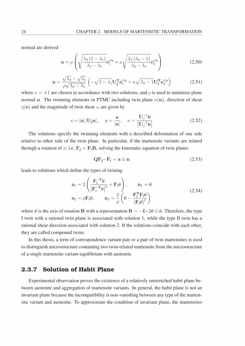
24 CHAPTER 2. MODELS OF MARTENSITIC TRANSFORMATION
normal are derived
a = ρ
⎛⎝√
λ3 (1− λ1)
λ3 − λ1
eeig1 + κ
√λ1 (λ3 − 1)
λ3 − λ1
eeig3
⎞⎠ (2.50)
n =
√λ3 −
√λ1
ρ√λ3 − λ1
(−√
1− λ1UTj e
eig1 + κ
√λ3 − 1UT
j eeig3
)(2.51)
where κ = ±1 are chosen in accordance with two solutions, and ρ is used to minimize plane
normal n. The twinning elements in PTMC including twin plane κ(n), direction of shear
η(a) and the magnitude of twin shear s, are given by
s = |a| |Ujn| , η =a
|a| , κ =U−1
j n∣∣U−1j n∣∣ (2.52)
The solutions specify the twinning elements with a described deformation of one side
relative to other side of the twin plane. In particular, if the martensite variants are related
through a rotation of π, i.e. Fj = FiR, solving the kinematic equation of twin planes
QFj−Fi = a⊗ n (2.53)
leads to solutions which define the types of twining
a1 = 2
(F−T
i e∣∣F−Ti e∣∣2 + Fie
), n1 = e
a2 = ρFie, n2 =2
ρ
(e− FT
i Fie
|Fie|2) (2.54)
where e is the axis of rotation R with a representation R = −I+2e⊗ e. Therefore, the type
I twin with a rational twin plane is associated with solution 1, while the type II twin has a
rational shear direction associated with solution 2. If the solutions coincide with each other,
they are called compound twins.
In this thesis, a term of correspondence variant pair or a pair of twin martensites is used
to distinguish microstructure containing two twin-related martensite from the microstructure
of a single martensite variant equilibrium with austenite.
2.3.7 Solution of Habit Plane
Experimental observation proves the existence of a relatively unstretched habit plane be-
tween austenite and aggregation of martensite variants. In general, the habit plane is not an
invariant plane because the incompatibility is non-vanishing between any type of the marten-
site variant and austenite. To approximate the condition of invariant plane, the martensites
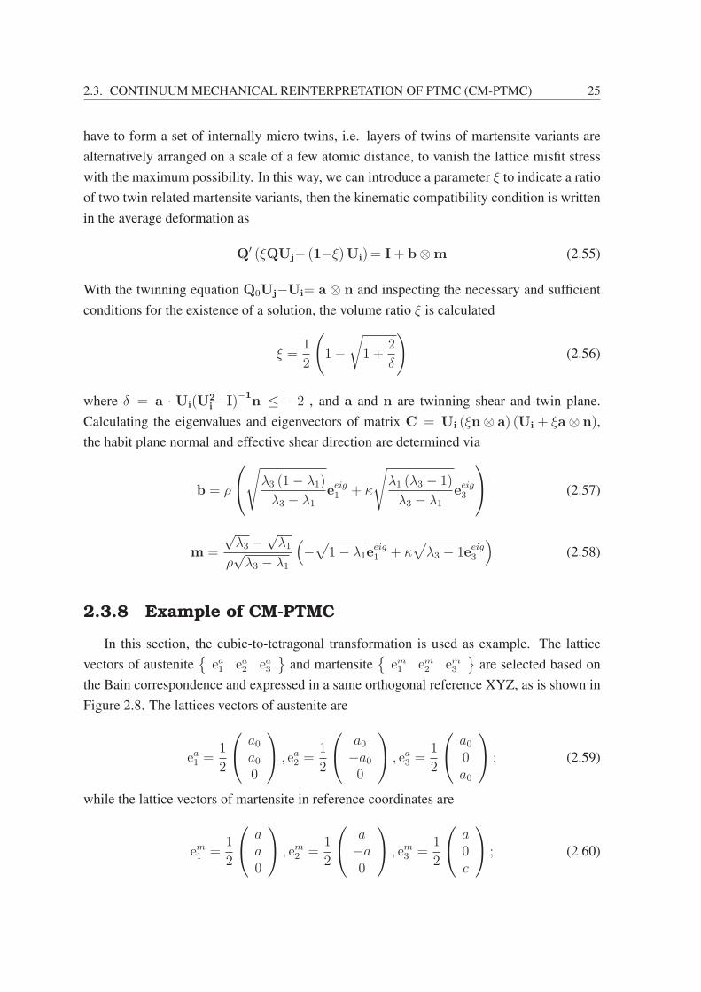
2.3. CONTINUUM MECHANICAL REINTERPRETATION OF PTMC (CM-PTMC) 25
have to form a set of internally micro twins, i.e. layers of twins of martensite variants are
alternatively arranged on a scale of a few atomic distance, to vanish the lattice misfit stress
with the maximum possibility. In this way, we can introduce a parameter ξ to indicate a ratio
of two twin related martensite variants, then the kinematic compatibility condition is written
in the average deformation as
Q′ (ξQUj− (1−ξ)Ui)= I+ b⊗m (2.55)
With the twinning equation Q0Uj−Ui= a ⊗ n and inspecting the necessary and sufficient
conditions for the existence of a solution, the volume ratio ξ is calculated
ξ =1
2
(1−√1 +
2
δ
)(2.56)
where δ = a · Ui(U2i −I)
−1n ≤ −2 , and a and n are twinning shear and twin plane.
Calculating the eigenvalues and eigenvectors of matrix C = Ui (ξn⊗ a) (Ui + ξa⊗ n),
the habit plane normal and effective shear direction are determined via
b = ρ
⎛⎝√
λ3 (1− λ1)
λ3 − λ1
eeig1 + κ
√λ1 (λ3 − 1)
λ3 − λ1
eeig3
⎞⎠ (2.57)
m =
√λ3 −
√λ1
ρ√λ3 − λ1
(−√1− λ1e
eig1 + κ
√λ3 − 1eeig3
)(2.58)
2.3.8 Example of CM-PTMC
In this section, the cubic-to-tetragonal transformation is used as example. The lattice
vectors of austenite{
ea1 ea2 ea3}
and martensite{em1 em2 em3
}are selected based on
the Bain correspondence and expressed in a same orthogonal reference XYZ, as is shown in
Figure 2.8. The lattices vectors of austenite are
ea1 =1
2
⎛⎝ a0
a00
⎞⎠ , ea2 =
1
2
⎛⎝ a0
−a00
⎞⎠ , ea3 =
1
2
⎛⎝ a0
0a0
⎞⎠ ; (2.59)
while the lattice vectors of martensite in reference coordinates are
em1 =1
2
⎛⎝ a
a0
⎞⎠ , em2 =
1
2
⎛⎝ a
−a0
⎞⎠ , em3 =
1
2
⎛⎝ a
0c
⎞⎠ ; (2.60)

26 CHAPTER 2. MODELS OF MARTENSITIC TRANSFORMATION
Figure 2.7: Schematic drawing of the internal twin and habit plane
where a0 is the lattice parameter of austenite and a and c are parameters relative to lattice of
martensite. Since MT is described by using deformation, there must be a stretch U homoge-
neously deforming the austenite lattice to the martensite one, with a mathematical expression
em=U3ea, with U3 =
⎛⎝ α 0 0
0 α 00 0 β
⎞⎠ (2.61)
where α = a/a0, β=c/a0. The diagonal matrix U3 indicates that the principle axes coincide
with the edges of the cubic unit cells, and the diagonal components of stretch matrix of are
eigenvalues of deformation gradients. In cubic-to-tetragonal transformation, there are three
different stretch matrices associated with three Bain correspondence relevant martensite vari-
ants. By inspecting the elements in the point group of m3m, two other stretch matrices are
U1 =
⎛⎝ β 0 0
0 α 00 0 α
⎞⎠ ,U2 =
⎛⎝ α 0 0
0 β 00 0 α
⎞⎠ (2.62)
If the twinning of martensite variants 1 and 2 with stretch matrices U1 and U2 is con-
sidered, we can verify the existence of the 180◦ rotation R about e =1√2
⎛⎝ 1
10
⎞⎠ to make
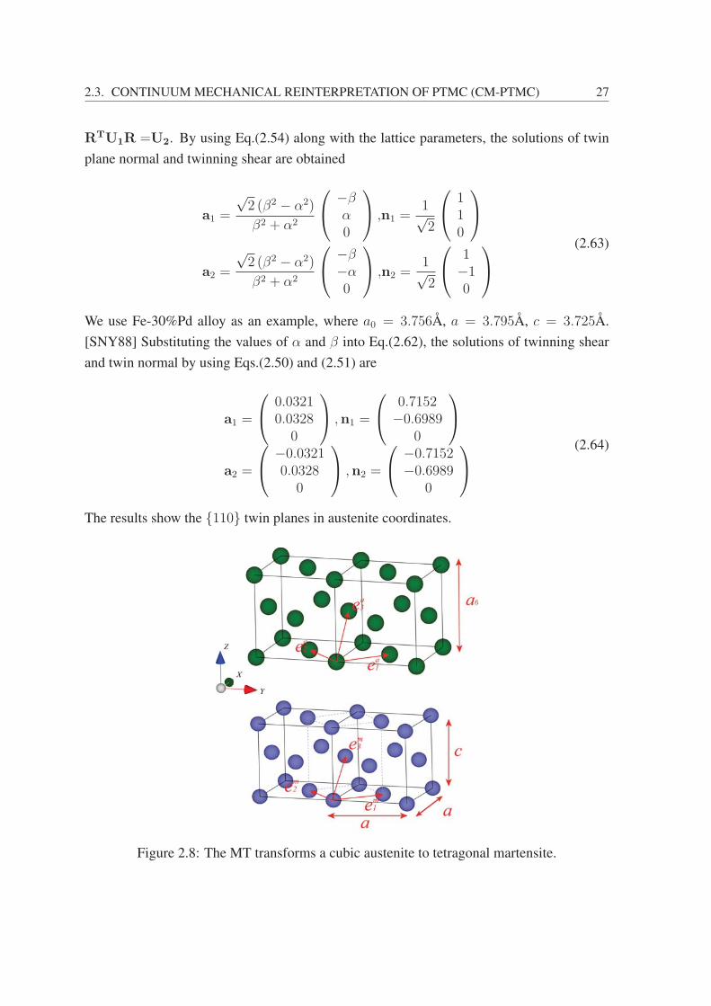
2.3. CONTINUUM MECHANICAL REINTERPRETATION OF PTMC (CM-PTMC) 27
RTU1R =U2. By using Eq.(2.54) along with the lattice parameters, the solutions of twin
plane normal and twinning shear are obtained
a1 =
√2 (β2 − α2)
β2 + α2
⎛⎝ −β
α0
⎞⎠ ,n1 =
1√2
⎛⎝ 1
10
⎞⎠
a2 =
√2 (β2 − α2)
β2 + α2
⎛⎝ −β
−α0
⎞⎠ ,n2 =
1√2
⎛⎝ 1
−10
⎞⎠
(2.63)
We use Fe-30%Pd alloy as an example, where a0 = 3.756Å, a = 3.795Å, c = 3.725Å.
[SNY88] Substituting the values of α and β into Eq.(2.62), the solutions of twinning shear
and twin normal by using Eqs.(2.50) and (2.51) are
a1 =
⎛⎝ 0.0321
0.03280
⎞⎠ ,n1 =
⎛⎝ 0.7152
−0.69890
⎞⎠
a2 =
⎛⎝ −0.0321
0.03280
⎞⎠ ,n2 =
⎛⎝ −0.7152
−0.69890
⎞⎠
(2.64)
The results show the {110} twin planes in austenite coordinates.
Figure 2.8: The MT transforms a cubic austenite to tetragonal martensite.
28 CHAPTER 2. MODELS OF MARTENSITIC TRANSFORMATION
2.3.9 Geometrically Linear Model with Infinitesimal Strain
The geometrically nonlinear elastic model of MT based on the deformation gradient
provides mathematically accurate solutions for the microstructural features. However, the
geometrical nonlinearity also brings in the complexity when the physical nonlinearity is
taken into consideration in modeling. The physical nonlinearity includes the anharmonic
energy density, which is no longer quadratic form in terms of strain, and nonlinear dynamics
that microstructure follows to evolve. Because of that, the linear approximation is a long term
using strategy to overcome the difficulties in geometrical nonlinearity in solid mechanics.
The linearized geometry simplifies the modeling of microstructural features in MT, providing
a not accurate but effective approximation due to the irrational indices of characteristic plane
and normal in martensites and/or austensite.
As is mentioned in section 2.3, the Lagrangian finite strain tensor with geometrical non-
linearity is written as
e =1
2
(FTF− I
)=
1
2
(∂ui
∂xj
+∂uj
∂xi
+∑k
∂uk
∂xi
∂uk
∂xj
)(2.65)
wherein the displacement gradient ∇u is defined as the matrix of the partial derivatives of the
displacement with the component (∇u)ij =∂ui
∂xj
. If the nonlinear term of the cross product
in Eq.(2.65) is neglected based on the fact that the displacement gradient in solid state phase
transformation is small enough, the infinitesimal strain tensor can be expressed as
e =1
2
(∂ui
∂xj
+∂uj
∂xi
)=
1
2
(FT + F−2I
)=
1
2
[∇u+(∇u)T
](2.66)
Applying the approximation to a rotation, the skew matrix (anti-symmetric rotation tensor)
in geometrically linear theory reads
w =1
2
(∂ui
∂xj
− ∂uj
∂xi
)=
1
2
(F−FT
)(2.67)
Since the stretch and rotation are approximated as follows
U ≈ I+ e, Q ≈ I+w (2.68)
the polar decomposition of the multiplying rotation and stretch is accordingly simplified by
adding anti-symmetric rotation to linear strain and identity, i.e.
F = I+∇u = I+ e+w (2.69)
And the materials symmetry of energy is expressed in strain as
ϕ(RTeR,T
)=ϕ (e,T) , for any rotation R ∈ P (e◦i ) (2.70)
2.3. CONTINUUM MECHANICAL REINTERPRETATION OF PTMC (CM-PTMC) 29
Substituting the Eq.(2.69) into the Eq.(2.37), the kinematic compatibility equation in ge-
ometrically linear elastic model is expressed in the independent variables of displacement
gradient.
(∇u)I − (∇u)J = a⊗ n (2.71)
Considering infinitesimal strain in Eq.(2.66), the strain compatibility equation widely uti-
lized in the geometrically linear elastic model of MT is derived
eI − eJ =1
2(a⊗ n+ n⊗ a) (2.72)
And the skew matrices satisfy
wI −wJ =1
2(a⊗ n− n⊗ a) (2.73)
With the strain compatibility equation, the twin plane normal and the twinning shear can be
determined by solving the eigenvalues and eigenvectors of E = eI−eJ =1
2(a⊗ n+ n⊗ a).
Sorting the eigenvalues of E by assuming ε1 ≤ ε2 ≤ ε3, and when the eigenvalues satisfy
ε1 ≤ 0, ε2 = 0, ε3 ≥ 0, there are two solutions of twinning shear and twin plane normal
a =√
2 (ε3 − ε1)(κ√−ε1e
eig1 +
√ε3e
eig3
)n =
1√(ε3 − ε1)
(−κ√−ε1e
eig1 +
√ε3e
eig3
) (2.74)
Similar to the analysis of the twinned martensite variants related by the 180◦ rotation with
the axis e, two sets of solutions corresponding to the type I and type II twins are available,
which read
a1 = 4 [(e · eI e) e− eI e] , n1 = e
a2 = 4 |(e · eI e) e− eI e| e, n2 =(e · eI e) e− eI e
|(e · eI e) e− eI e|(2.75)
The invariant plane between austenite and single martensite is solved by using the same
procedures with the equation
E = eI − 0 =1
2(a⊗ n+ n⊗ a) (2.76)
Based on the solved twin plane normal and shear direction, the habit plane normal and the
shear direction of the average deformation is calculated by using
ξej− (1−ξ) ei=1
2(b⊗m+m⊗ b) (2.77)
if the one eigenvalue of the average strain ξej− (1−ξ) ei is equal to zero with an appropriate
chosen value of ξ. The more detailed procedures is referenced in [Bha03].

30 CHAPTER 2. MODELS OF MARTENSITIC TRANSFORMATION
2.4 Landau Theory with IRS
Detailed in the previous sections, the prototype PTMC and CM-PTMC theories achieve
great success in illuminating the static microstructure features of a material undergoing MT
by unveiling the crucial effect of the kinematic compatibility. Integrated with the wisdom
of group theory, crystallography, and matrix algebra, most of intriguing microstructural pat-
terns, including wedge-like, herringbone, etc. [Bha03] more than habit planes and twin
boundaries, are elaborately analyzed in mathematics. However, the static model is limited
to understand the stable morphology of martensites. It fails to capture most of meta-stable
microstructural features governed by dynamics. Moreover, the temperature relevant thermo-
dynamic and thermomechanical behaviors, such as shape memory effects and temperature
dependent hysteresis of stress-strain curve in SMAs, acoustic phonon softening, varying
driving force with temperature, etc., are not taken into consideration in PTMC theories.
Therefore, a dynamical modeling is required.
Among the phenomenological approaches, Landau theory not only provides an excel-
lent interpretation for the formation of static patterns in phase transition, but has ability to
integrate with various dynamic formulism to explain fascinating dynamic behaviors. The
born of Landau type model for first-order displacive transformation with Irreducible Repre-
sentation form of Strains (IRS) was traced back to 1970s, when the progress of the renor-
malization group technique enabled Landau theory to approximately handle the problem
of fluctuations on critical phenomena. Cook [Coo76] interpreted the fluctuations as large
amplitude, quasi-static wave packets to extend the Landau’s theory of second-order phase
transition to first-order structural transition. With a justified hypothesis that systems having
the same symmetry were expected to have similar critical properties, Cowley [Cow76] ap-
plied these ideas to a static analysis of the first-order structural phase transition triggered by
homogeneous deformation and included the effect of fluctuations. He creatively connected
fluctuation in lattice dynamics with the stability of crystals against deformation in macro-
scopic elasticity by inspecting the velocities of acoustic waves and irreducibly representing
them as the functional of the linear combination of elastic constants. In his static analysis,
the homogeneous deformations were written in Landau polynomial expanded to forth or-
der with homogeneous strain as a primary Order Parameter(OP). The fluctuation of elastic
heterogeneity entered Hamiltonian via the strains with nonzero wave vectors in reciprocal
space.

2.4. LANDAU THEORY WITH IRS 31
2.4.1 Landau Free Energy
Realizing the Landau model has advantages of yielding the whole temperature dependent
physical nonlinearity, Falk [Fal80, Fal82] initiatively proposed Landau model accounting for
thermodynamic and thermomechanical behaviors of MT in SMAs. With the temperature de-
pendent Landau polynomial expanded in strain up to sixth order, the model of temperature
induced MT in one-dimensional homogeneous medium qualitatively derived the tempera-
ture dependent thermodynamic properties and shape memory behaviors, such as the latent
heat in transformation, the stress-strain curves at various temperatures (especially the hys-
teresis below critical temperature), the lattice softening, the stress effect on the temperature-
induced phase transition, etc. Afterwards, the one-dimensional Landau potential was applied
to different structural transitions, and the various solutions of domain walls characterized in
soliton, kink or periodon, were also analyzed [Fal83, SS03, SSL01], which are directly as-
sociated with the morphology of twinned or single martensite in the subsequent chapters.
To extend the one-dimensional Landau free energy to 2D or 3D phase transformations,
the free-energy function should be expanded to anharmonic terms with the OPs of a second-
rank tensor of strain, and be kept invariant with respect to the operations in the high symmetry
group of parent phase. However, the requirement of identifying the broken symmetry in
crystallography and representing them in Landau free energy renders the determination of
OPs difficult. To overcome the difficulty, the method of irreducible representation of the
more symmetric, high temperature phase was naturally incorporated, in which appropriate
combinations of the components of strain tensor (in IRS form) were adopted as OPs. The
great success of identification of the IRS OPs and the determination of the analytic form
of the Landau free energy for all the structural phase transitions were credited to Toledano
and Toledano [TFA83, TT80], Likaos[LS82], Salje[Sal90], Stokes[SH84] and Hatch[HS84,
HLSS03]. The details of the irreducible representation theory and the application to the
construction of Landau energy can refer to the textbook [TD96]. Herein, only the general
methodology is briefly introduced.
Since the Landau energy density for MT is in terms of strain components and keep in-
variant under any symmetry operation R in the point group of austenite, we have
e′ =RTeR F ′ (e′, T ) = F (e, T ) (2.78)
Provided the strain tensor written in Cartesian coordinates with orthogonal bases e0i is
⎛⎝ ε11 ε12 ε13
ε12 ε22 ε23ε13 ε23 ε33
⎞⎠ (2.79)
32 CHAPTER 2. MODELS OF MARTENSITIC TRANSFORMATION
the strain tensor can be represented as a vector in a six-dimensional space S spanned by ϕi
using Voigt notation. ⎛⎜⎜⎜⎜⎜⎜⎝
ε1ε2ε3ε4ε5ε6
⎞⎟⎟⎟⎟⎟⎟⎠
=
⎛⎜⎜⎜⎜⎜⎜⎝
ε11ε22ε33
ε23 + ε32ε13 + ε31ε12 + ε21
⎞⎟⎟⎟⎟⎟⎟⎠
,
ϕ1 = e01 ⊗ e01ϕ2 = e02 ⊗ e02ϕ3 = e03 ⊗ e032ϕ4 = e02 ⊗ e03+e03 ⊗ e022ϕ5 = e01 ⊗ e03+e03 ⊗ e012ϕ6 = e01 ⊗ e02+e02 ⊗ e01
(2.80)
Thus, the symmetry operations Rij of the point group are represented as rMN to keep the
identity
εM′ = rMNεN (2.81)
Since the representation rMN is reducible into the irreducible representation, the symmetry
adapted strains are expressed as the linear combination of strain components, and strain
space S is accordingly decomposed into the subspaces spanned by the direction vectors of
symmetry adapted strains, namely
e1 =1√3(ε11 + ε22 + ε33)
e2 =1√2(ε11 − ε22)
e3 =1√6(ε11 + ε22 − 2ε33)
e4 = (ε23 + ε32)e5 = (ε13 + ε31)e6 = (ε12 + ε21)
S1 (dialtation) ψ1 = ϕ1 + ϕ2 + ϕ3
S12 (deviatoric) ψ2 = ϕ1 − ϕ2
ψ3 = ϕ1 + ϕ2 − 2ϕ3
S25 (shear)
ψ4 = 2ϕ4
ψ5 = 2ϕ5
ψ6 = 2ϕ6
(2.82)

2.4. LANDAU THEORY WITH IRS 33
On the other hand, the Landau energy density is expanded in Taylor series with respect
to strains
F (e, T ) = F 0 (T ) + F 1 (e, T ) + F 2 (e, T ) + ... (2.83)
Since the nth degree in Landau polynomial of MT is written as the scalar product of nth
elastic constants C and strains e, elastic constants C can be decomposed into the sum of
the product of symmetry adapted elastic constant F nj (linear combination of nth order elastic
constants) and invariant direction in a symmetrised product space according to the same
irreducible representation. On each invariant direction, there is an invariant Jnj expressed as
polynomial of strain components. So that, the nth degree in Landau energy expansion reads
F n (e, T ) =∑j
F nj J
nj (2.84)
Falk has summarized parts of the strain invariants listed in Tables(1-2) of [FK90]. Based
on these, the Landau energy for specific MT is constructed by selecting the invariants and
truncating at an appropriate high order term. The Landau free energy for typical MTs
are available in literature, for example the energy expression for cubic-to-tetragonal tran-
sition by Barsch and Krumhansl [BK84] and cubic-to-trigonal by [SLS10, Sal09], cubic-to-
orthorhombic by [NK82, SLS10, SSF12] and cubic-monoclinic I by [FK90, SLS10, SSF12].
2.4.2 Dynamics
Fascinating dynamic behaviors during MTs can be revealed when the Landau energy
is equipped with different dynamic formalisms. The Landau energy based on the IRS is
suitable for most of dynamics, including static stress equilibrium, TDGL, Bales-Gooding
and displacement based Lagrange-Rayleigh dynamics, etc. [LSR+03] The representative
achievements on depicting dynamic phenomena, such as the near-sound velocity of propa-
gation of domain walls and ’dynamical twinning’, attribute to the inertia dynamics, either
Bales-Gooding type or Lagrange-Rayleigh type. The inertia dynamics has a distinctive fea-
ture of including kinetic energy to account for inertial effects of material point in real space
or elastic oscillators with different wave vectors in reciprocal space. Sometimes, a Rayleigh
dissipation term is additionally incorporated representing the sound-wave viscosity. Two
formulations of inertia dynamics, i.e. Bales-Gooding in strains or Lagrange-Rayleigh in
displacement, differ in the deductions of dynamic equations. The Bales-Gooding dynamics
works only with strain fields, in which the Lagrangian is written in primary OP strain(s) and
explicitly appends the St. Venant’s compatibility constraint via a Lagrange multiplier. The
procedure yields an anisotropic long-range kernel indicating the preferential orientation of
twinning. While in displacement based Lagrange-Rayleigh dynamics, a general equation

34 CHAPTER 2. MODELS OF MARTENSITIC TRANSFORMATION
of motion is straightforwardly obtained from Lagrange mechanics by implementing varia-
tion of Lagrangian with respect to displacement or displacement gradient field, in which the
displacement are served as independent variables.
2.4.3 Motions of Domain Walls
The first issue the inertia dynamics settled in MT is the movement of domain walls.
Barsch and Krumhansl [BK84, BG91] included anharmonic strain energy and nonlocal con-
tribution of strain gradient to formulate inhomogeneous strain fields associated with hetero-
geneity of martensites and domain boundaries. The results of motion equations either in
Lagrange mechanics involving displacement or Bales-Gooding dynamics led to the same
kinked solitary wave solution describing the moving twin boundaries that separate alterna-
tively arranged martensite variants. These soliton solution was further evidenced by Jabcob
and Curnoe in their 2D (3D) calculations of strain fields after square-rectangular (cubic-
tetragonal) MT [Jac85, CJ00]. The ’dynamical twinning’, different from the classical ar-
gument that dislocations stabilize twinned structure, revealed a different physical scenario
that the long-range elastic interaction in austenite with a kinetic energy renders a dispersion
giving rise to twinned structure [BHK87]. Attempting to minimize the kinetic energy, a
perpetually propagation of twinning interfaces through the system is energetically and dy-
namically favored. The ’dynamical twinning’ provides a new perspective to study the shape
memory effect and autocatalytic twinning.
2.4.4 Precursors
The nucleation and the formation of precursors are two other topics of nonlinear Lan-
dau model. The combination of anharmonic Landau energy with strain gradient and iner-
tia dynamics gives an ingenious physical scenario beyond the classical nucleation theory
[SLSB99, LSD+00]. Looking back to the beginning of Section 2.4, Cook [Coo76] argued
that a high density of the hetero-phase fluctuations in a system with anharmonic energy
interplaying with interface energy would lead to the formation of precursor above the crit-
ical temperature, whereas it nucleates into low symmetric phase at the temperature below
the coherent transformation point. The statement was further clarified by Krumhansl and
Gooding [KG89] that the anomalous low values of elastic constants or in phonon dispersion
were discovered in a few directions, rather than harmonic instability of soft-mode, which
accounted for the intrinsic features of precursors and were associated with ’central peaks’.
Kartha [KKSW95] simulated the meso-scale tweed pattern and interpreted its formation by
introducing the concept of the static long-range elastic kernel in a heterogeneous system.
2.4. LANDAU THEORY WITH IRS 35
The tweed, recognized as a distinct thermodynamically meta-stable phase, is mediated by
the coupling between strain dependent anharmonic energy and spatial dependent nonlocal
strain gradient [BK88]. In a modern statement considering inertia dynamics by Lookman
[LSR+03], the elastic oscillators have different ’strain-mass’ densities ρ(k) ∼ 1/k2 and
damping 1/ρ(k) ∼ k2, such that the lighter large-k oscillators equilibrate first, correspond-
ing to earlier formation of smaller-scale oriented tweed. The following nucleation to form
the twinned pattern or other microstructure can be achieved by autocatalysis mechanism with
a varying localized stress, which will be detailed in Chapter 4.
2.4.5 Microstructure Simulation
With the development of the computer science, the dream of representing the temporal
evolution of microstructure is turned into reality. Kartha [KKSW95] carried out a Monte
Carlo simulation with Landau free energy to represent the microstructure of tweed and
twins during the square-to-rectangular MT. Jacob [Jac95] simulated the static morphol-
ogy of the same transformation in a constrained system, while the TDGL simulation us-
ing OP strains and long-range compatibility kernel was found in [SLSB99]. The displace-
ment based underdamped Lagrange-Rayleigh dynamics was also applied to 2D simulations
analogs of tetragonal-to-orthorhombic and hexagonal-to-orthorhombic ferroelastic transfor-
mations [CJ01a, CJ01b]. Ahluwalia [AA01] included a coupling term between squares of
the OP strains in Landau free energy and dropped the non-OP strains in Bales-Gooding
formalism to represent the avalanches in MT. Most of 3D simulations of microstructural
evolution were utilizing displacement based Lagrange dynamics, like the cubic-to-tetragonal
ferroelastics in [LSR+03, ALS06], with the exceptions of Rasmussen and Shenoy who con-
sidered the St. Venant’s compatibility constraint in three dimension in strain based over-
damped equation. The most intriguing discovery in microstructure simulation is the richness
of morphology which were formed due to the selective transformation paths in different dy-
namics, for example the hierarchical microstructure of tweed, twin and chessboard patterns
[SLSB99, SSB+98] and ’maze’ like pattern with ’zoom lens’ moving boundaries in the in-
termediate state of transformation [LSR+03].
In the following subsections, the nonlinear Landau model with displacement based La-
grange - Rayleigh dynamics are detailed. Especially, the simulation procedures, numerical
strategy and results of the 3D simulations are presented with the examples of the Fe-Pd alloy
for cubic-to-tetragonal MT and Au-Cd alloy for cubic-to-trigonal MT. It is known that the
constructions of Lagrangian and dynamic equations are two key issues in modeling. The
36 CHAPTER 2. MODELS OF MARTENSITIC TRANSFORMATION
Lagrangian is defined as
L=
∫V
dr {T − f} (2.85)
where f is Landau free energy density with the expression f = flocal+fnon−OP +fgrad. The
individual energy density contributions are expanded in terms of symmetry adapted strain
following the strategy in subsection 2.4.1. With geometrically linear approximation, the
symmetry adapted strain can be directly linked with the displacements by
ei = λ(i)kj εkj = λ
(i)kj
(∂uk
∂xj
+∂uj
∂xk
)(2.86)
where, λkj is the symmetry related coefficient to keep that the energy is invariant. For exam-
ple, 1/√
2 and −1/√
2 are adopted as the coefficients of ε11 and ε22 in the expression of e2,
see Eq. (2.82).
The kinetic energy density T is also linked with displacement and written as
T =ρ
2
N−dim∑i
ui(r, t)2
(2.87)
where ρ is mass density. The incorporation of kinetic energy is capable of describing the
inertial effect of the finite velocity of interface motion. The near sound velocity indicates the
rates of strain evolution in position space and associates with the propagation of the acoustic
waves in Fourier space.
In a system consisting of kinetic and potential energies, the internal friction plays a cru-
cial role in dissipating the excess energy and drives the system towards the energy minima of
martensitic state. With the friction, the motion of elastic oscillators as a result of the kinetic
energy gained from the lowered Landau energy in phase transformation is certainly damped.
Consequently, a simple Rayleigh dissipation density can be included to describe the elastic
viscosity, with the mathematical expression as square summation of strain velocity for all the
OP strains with viscosity parameter γ
R =n−OP∑
i
γi2e2i (r, t) (2.88)
It is noteworthy that the system is energetic conserved if the Rayleigh dissipation term is
removed, such that the system oscillates indefinitely.
With a constructed Lagrangian, the time evolution of the microstructure is implemented
by numerically solving the Lagrange-Rayleigh equation
d
dt
δL
δUi
− δL
δUi
= −δR
δUi
(2.89)

2.4. LANDAU THEORY WITH IRS 37
2.4.6 Chain Rule for Functional Differentiation
Before deriving the general equation of motion from Lagrange-Rayleigh equation, we
have to prove that the chain rule is also applied to the functional differentiation, i.e.
δF
δQi
=∑k
δF
δqk
∂qk∂Qi
(2.90)
where F =
∫r
I [Qi,∇Qi, q (Qi,∇Qi)] dr, and I denotes the full integrand of Landau en-
ergy density.
In the proof, we simplify the Lagrange-Rayleigh equation to the static limit, i.e. the
inertia (on the left) and the real damping (second right) parts are removed. By doing so, the
dynamic equation is degenerated into the static equation of stress equilibrium. Generally, the
equilibrium solution can be found by implementing the variation of F (including a gradient
regularization) with respect to variables Qi, which reads
δF
δQi
=∂I
∂Qi
−∇ ∂I
∂∇Qi
= 0 (2.91)
If the variables Qi are obtained via an unambiguous transformation T [·] of the variables qj ,
i.e. Q = T [q] , the inverse transformation must be expressed as q = T−1 [Q]. Thus, the
derivatives in Eq.(2.91) can be expanded via the chain rule as
∂I
∂Qi
=∑k
∂I
∂qk
∂qk∂Qi
+∂I
∂∇qk
∂∇qk∂Qi
∇ ∂I
∂∇Qi
= ∇[∑
k
∂I
∂qk
∂qk∂∇Qi
+∂I
∂∇qk
∂∇qk∂∇Qi
] (2.92)
It is then easy to reformulate the Eq.(2.91) with these two summations as follows,
δF
δQi
=∑k
∂I
∂qk
∂qk∂Qi
+∑k
∂I
∂∇qk
∂∇qk∂Qi
−∑k
∇(
∂I
∂qk
∂qk∂∇Qi
)
−∑k
(∇ ∂I
∂∇qk
)∂∇qk∂Qi
−∑k
∂I
∂∇qk
(∇ ∂∇qk∂∇Qi
) (2.93)
Because Q and q are related by a spatial independent transformation T , it is clear that∂qk
∂∇Qi
= 0. Therefore, the third sum in the above equation is equal to 0, and then
δF
δQi
=∑k
[∂I
∂qk
∂qk∂Qi
−(∇ ∂I
∂∇qk
)∂∇qk∂∇Qi
]+∑k
∂I
∂∇qk
[∂∇qk∂Qi
−∇ ∂∇qk∂∇Qi
](2.94)
38 CHAPTER 2. MODELS OF MARTENSITIC TRANSFORMATION
Using the chain rule again leads to the relationships of
∇qk =∑i
∂qk∂Qi
∇Qi
∂∇qk∂∇Qi
= ∂∑j
∂qk∂Qj
∇Qj/∂∇Qi =∂qk∂Qi
(2.95)
Thus, the first sum in Eq(2.94) is compressed as∑k
(∂I
∂qk−∇ ∂I
∂∇qk
)∂qk∂Qi
In addition, a set of similar relationships
∂∇qk∂Qi
= ∂∑j
∂qk∂Qj
∇Qj/∂Qi =∑j
∂2qk∂Qi∂Qj
∇Qj
∇ ∂qk∂Qi
=∂∇qk∂Qi
=∑j
∂2qk∂Qi∂Qj
∇Qj
(2.96)
is obtained formally by utilizing chain rule of derivatives. It is apparent that second sum
would vanish in Eq(2.94), which leads to the conclusion that the chain rule of derivatives
also applies to the functional differentiation, viz.
δF
δQi
=∑k
(∂I
∂qk−∇ ∂I
∂∇qk
)∂qk∂Qi
=∑k
δF
δqk
∂qk∂Qi
(2.97)
In our particular case for the displacement field, let Qi = ui,j and qk = ek. The symmetry
adapted strain ek and the displacement gradient ui,j are linked via a matrix
ek = T−1k ui,j⎡
⎢⎢⎢⎢⎢⎢⎣
e1e2e3e4e5e6
⎤⎥⎥⎥⎥⎥⎥⎦=
⎡⎢⎢⎢⎢⎢⎢⎢⎣
1√3
1√3
1√3
0 0 01√2
−1√2
0 0 0 01√6
1√6
−2√6
0 0 0
0 0 0 1 0 00 0 0 0 1 00 0 0 0 0 1
⎤⎥⎥⎥⎥⎥⎥⎥⎦
⎡⎢⎢⎢⎢⎢⎢⎣
sym (u1,1)sym (u2,2)sym (u3,3)sym (u2,3)sym (u1,3)sym (u1,2)
⎤⎥⎥⎥⎥⎥⎥⎦
(2.98)
In 2D, the transformation matrix T is simplified as follow⎡⎣ e1
e2e3
⎤⎦ =
⎡⎣ 1/√
2 1/√
2
1/√
2 −1/√
21
⎤⎦⎡⎣ sym (u1,1)
sym (u2,2)sym (u1,2)
⎤⎦ (2.99)
Therefore,δF
δui,j
=∑k
(∂flandau∂ek
−∇∂flandau∂∇ek
)∂ek∂ui,j
=∑k
σk∂ek∂ui,j
.
By taking the functional differentiation along with the chain rule, the general equation of
motion in displacements is obtained.
ρui =∑k
σk∂ek∂ui,j
+∑k
σk∂ek∂ui,j
(2.100)

2.4. LANDAU THEORY WITH IRS 39
2.4.7 Numerical Strategy
The general equation of motion was numerically solved in a periodic 3D box by using a
operator-splitting-based, quasi-spectral, semi-implicit time stepping scheme in the following
subsections.
For simplicity,
∂2u
∂t2= f(u,∇u) (2.101)
The f(u,∇u) was the nonlinear term relevant to energy density. The variation of gradient
energy density, named Ginzburg term, was written as the functional of OP strains and treated
fully explicitly in Fourier space.
δ(∇ek)2
δek= −2∇2ek = 2k2ek (2.102)
During the time evolution, the nonlinear term was evaluated at each time step t, and the
acceleration was approximated by using central-difference formula
∂2ui
∂t2≈ ut+Δt
i − 2uti + ut−Δt
i
Δt2(2.103)
In this work, the anisotropic Rayleigh dissipation term was simplified into an isotropic vis-
cous term with the viscosity γ i.e.
δR
δui,j
= ∇ · ∂σ∂t
≈ γ∇2∂u
∂t(2.104)
Numerically, the viscous term was treated in semi-implicit form, and then transformed into
Fourier space.
γ∇2∂u
∂t≈ γ∇2
(ut+Δt − ut
Δt
)= −γk2
Δt
(ut+Δt − ut
)(2.105)
where, the implicit displacements at t + Δt step can be served as the linear term s[ut+Δt
]in numerical calculation. Otherwise, we can elaborately choose a linear term s
[ut+Δt
]=
s
(i∑1
(−1)iγik2iut+Δt
)adding to both sides of dynamic equation to tackle the numerical
instability, which had been used to solve the Cahn-Hilliard equation with composition de-
pendent mobility [ZCST99]. Reformulating the dynamic equation resulted in the following
explicit time-stepping scheme in the spectrum
ut+Δti =
(1 +
1
1 + γk2Δt
)uti −
1
1 + γk2Δtut−Δti +
(Δt)2
1 + γk2Δtf(ut, ut
i,j,∇etk)
(2.106)
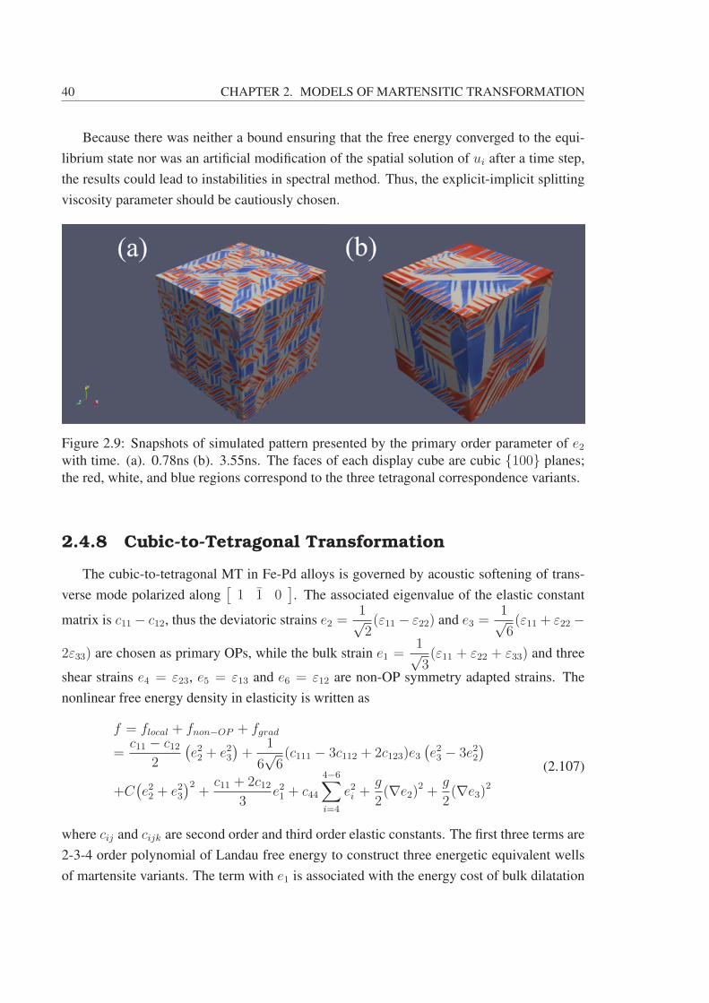
40 CHAPTER 2. MODELS OF MARTENSITIC TRANSFORMATION
Because there was neither a bound ensuring that the free energy converged to the equi-
librium state nor was an artificial modification of the spatial solution of ui after a time step,
the results could lead to instabilities in spectral method. Thus, the explicit-implicit splitting
viscosity parameter should be cautiously chosen.
Figure 2.9: Snapshots of simulated pattern presented by the primary order parameter of e2with time. (a). 0.78ns (b). 3.55ns. The faces of each display cube are cubic {100} planes;
the red, white, and blue regions correspond to the three tetragonal correspondence variants.
2.4.8 Cubic-to-Tetragonal Transformation
The cubic-to-tetragonal MT in Fe-Pd alloys is governed by acoustic softening of trans-
verse mode polarized along[1 1 0
]. The associated eigenvalue of the elastic constant
matrix is c11 − c12, thus the deviatoric strains e2 =1√2(ε11 − ε22) and e3 =
1√6(ε11 + ε22 −
2ε33) are chosen as primary OPs, while the bulk strain e1 =1√3(ε11 + ε22 + ε33) and three
shear strains e4 = ε23, e5 = ε13 and e6 = ε12 are non-OP symmetry adapted strains. The
nonlinear free energy density in elasticity is written as
f = flocal + fnon−OP + fgrad
=c11 − c12
2
(e22 + e23
)+
1
6√6(c111 − 3c112 + 2c123)e3
(e23 − 3e22
)+C(e22 + e23
)2+
c11 + 2c123
e21 + c44
4−6∑i=4
e2i +g
2(∇e2)
2 +g
2(∇e3)
2
(2.107)
where cij and cijk are second order and third order elastic constants. The first three terms are
2-3-4 order polynomial of Landau free energy to construct three energetic equivalent wells
of martensite variants. The term with e1 is associated with the energy cost of bulk dilatation

2.4. LANDAU THEORY WITH IRS 41
in transformation; the summation term is the shear energy density and the remaining are
nonlocal gradient terms.
For numerical simulation, it is proven that a system of 1283 cube size is eligible for
revealing the characteristic features in microstructure evolution. Since deviatoric strain e2 is
the primary OP which contributes greater than any other factor in cubic-to-tetragonal MT,
it is adopted to represent different martensitic domains. We present both transient and full
converged results of 3D structure in Figure 2.9. Three types of colored domains are easily
seen, i.e. red, blue and white ones in the structure snapshot, which represent three martensite
variants. The red one is of a positive magnitude of e2, while the blue one is negative and
the white one has the similar value of e2 as austenite. The austenite is not considered to be
retained here. The pattern reveals the nature of cubic-to-tetragonal MT with the walls lying
in cubic {110} planes to minimize dilatational and shear energy, which is consistent with
what CM-PTMC predicts in subsection 2.3.8. What to be highlighted is the length scale of
twinned martensites in transient state is smaller than that of converged martensites, which is
the result of energy minimization by eliminating the interface. Moreover, needle like twins
and collisions of identical/different variants can be found even for a long time simulation.
The morphology of tapering needle is favored by energy minimization. The slice of the
converged martensites with three variants is shown in Figure 2.10. Clearly, three martensite
variants have not equivalently grown. The microstructure consists of two primary bands,
here blue and white; each primary extends in[1 0 1
]direction and is penetrated by
the third variant, here red ones. At the top and bottom parts, only blue and white variants
organize the two-variant microstructure similar to that in 2D. The central part shows chevron
or herringbone patterns; some red domains are continuous across the blue-white boundaries,
where they bend through 90◦ and are slightly shrunk as well.
2.4.9 Cubic-to-Trigonal Transformation
From the CM-PTMC, we understand that the system undergoing cubic-to-trigonal MT
produces four martensite variants, with unique transformation stretch matrices as follows
U1 =
⎛⎝ α γ γ
γ α γγ γ α
⎞⎠ ,U2 =
⎛⎝ α −γ −γ
−γ α γ−γ γ α
⎞⎠ ;
U3 =
⎛⎝ α −γ γ
−γ α −γγ −γ α
⎞⎠ ,U4 =
⎛⎝ α γ −γ
γ α −γ−γ −γ α
⎞⎠
(2.108)
Because individual variants differ in the shear components of the strain tensors, the shear
strains e4, e5, and e6 are selected as primary OPs. The Landau polynomial depicting local
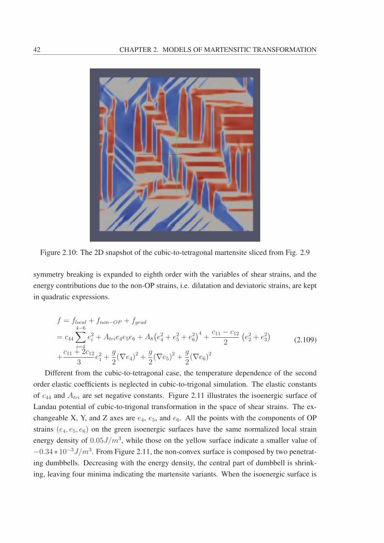
42 CHAPTER 2. MODELS OF MARTENSITIC TRANSFORMATION
Figure 2.10: The 2D snapshot of the cubic-to-tetragonal martensite sliced from Fig. 2.9
symmetry breaking is expanded to eighth order with the variables of shear strains, and the
energy contributions due to the non-OP strains, i.e. dilatation and deviatoric strains, are kept
in quadratic expressions.
f = flocal + fnon−OP + fgrad
= c44
4−6∑i=4
e2i + Atrie4e5e6 + A8
(e24 + e25 + e26
)4+
c11 − c122
(e22 + e23
)+c11 + 2c12
3e21 +
g
2(∇e4)
2 +g
2(∇e5)
2 +g
2(∇e6)
2
(2.109)
Different from the cubic-to-tetragonal case, the temperature dependence of the second
order elastic coefficients is neglected in cubic-to-trigonal simulation. The elastic constants
of c44 and Atri are set negative constants. Figure 2.11 illustrates the isoenergic surface of
Landau potential of cubic-to-trigonal transformation in the space of shear strains. The ex-
changeable X, Y, and Z axes are e4, e5, and e6. All the points with the components of OP
strains (e4, e5, e6) on the green isoenergic surfaces have the same normalized local strain
energy density of 0.05J/m3, while those on the yellow surface indicate a smaller value of
−0.34 ∗ 10−3J/m3. From Figure 2.11, the non-convex surface is composed by two penetrat-
ing dumbbells. Decreasing with the energy density, the central part of dumbbell is shrink-
ing, leaving four minima indicating the martensite variants. When the isoenergic surface is
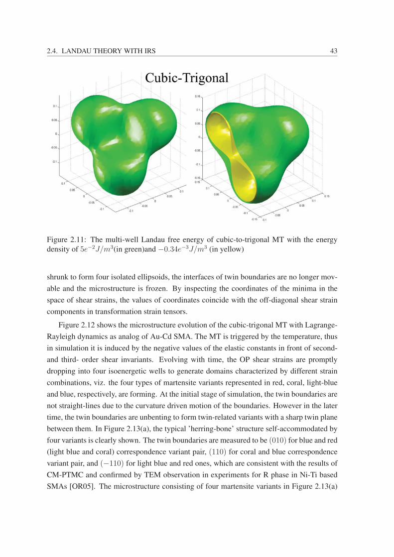
2.4. LANDAU THEORY WITH IRS 43
Figure 2.11: The multi-well Landau free energy of cubic-to-trigonal MT with the energy
density of 5e−2J/m3(in green)and −0.34e−3J/m3 (in yellow)
shrunk to form four isolated ellipsoids, the interfaces of twin boundaries are no longer mov-
able and the microstructure is frozen. By inspecting the coordinates of the minima in the
space of shear strains, the values of coordinates coincide with the off-diagonal shear strain
components in transformation strain tensors.
Figure 2.12 shows the microstructure evolution of the cubic-trigonal MT with Lagrange-
Rayleigh dynamics as analog of Au-Cd SMA. The MT is triggered by the temperature, thus
in simulation it is induced by the negative values of the elastic constants in front of second-
and third- order shear invariants. Evolving with time, the OP shear strains are promptly
dropping into four isoenergetic wells to generate domains characterized by different strain
combinations, viz. the four types of martensite variants represented in red, coral, light-blue
and blue, respectively, are forming. At the initial stage of simulation, the twin boundaries are
not straight-lines due to the curvature driven motion of the boundaries. However in the later
time, the twin boundaries are unbenting to form twin-related variants with a sharp twin plane
between them. In Figure 2.13(a), the typical ’herring-bone’ structure self-accommodated by
four variants is clearly shown. The twin boundaries are measured to be (010) for blue and red
(light blue and coral) correspondence variant pair, (110) for coral and blue correspondence
variant pair, and (−110) for light blue and red ones, which are consistent with the results of
CM-PTMC and confirmed by TEM observation in experiments for R phase in Ni-Ti based
SMAs [OR05]. The microstructure consisting of four martensite variants in Figure 2.13(a)
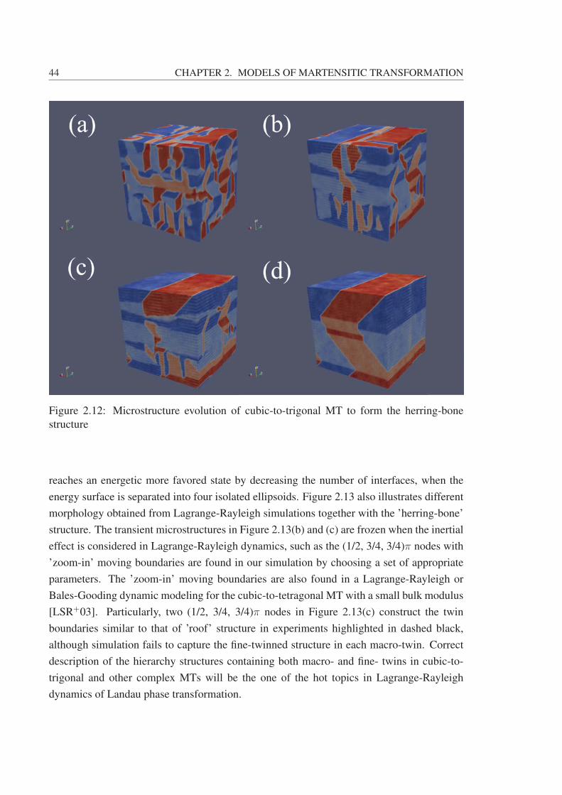
44 CHAPTER 2. MODELS OF MARTENSITIC TRANSFORMATION
Figure 2.12: Microstructure evolution of cubic-to-trigonal MT to form the herring-bone
structure
reaches an energetic more favored state by decreasing the number of interfaces, when the
energy surface is separated into four isolated ellipsoids. Figure 2.13 also illustrates different
morphology obtained from Lagrange-Rayleigh simulations together with the ’herring-bone’
structure. The transient microstructures in Figure 2.13(b) and (c) are frozen when the inertial
effect is considered in Lagrange-Rayleigh dynamics, such as the (1/2, 3/4, 3/4)π nodes with
’zoom-in’ moving boundaries are found in our simulation by choosing a set of appropriate
parameters. The ’zoom-in’ moving boundaries are also found in a Lagrange-Rayleigh or
Bales-Gooding dynamic modeling for the cubic-to-tetragonal MT with a small bulk modulus
[LSR+03]. Particularly, two (1/2, 3/4, 3/4)π nodes in Figure 2.13(c) construct the twin
boundaries similar to that of ’roof’ structure in experiments highlighted in dashed black,
although simulation fails to capture the fine-twinned structure in each macro-twin. Correct
description of the hierarchy structures containing both macro- and fine- twins in cubic-to-
trigonal and other complex MTs will be the one of the hot topics in Lagrange-Rayleigh
dynamics of Landau phase transformation.
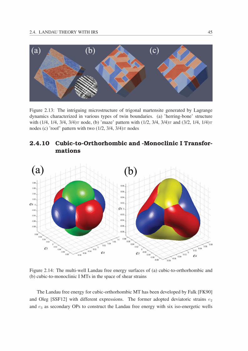
2.4. LANDAU THEORY WITH IRS 45
Figure 2.13: The intriguing microstructure of trigonal martensite generated by Lagrange
dynamics characterized in various types of twin boundaries. (a) ’herring-bone’ structure
with (1/4, 1/4, 3/4, 3/4)π node, (b) ’maze’ pattern with (1/2, 3/4, 3/4)π and (3/2, 1/4, 1/4)πnodes (c) ’roof’ pattern with two (1/2, 3/4, 3/4)π nodes
2.4.10 Cubic-to-Orthorhombic and -Monoclinic I Transfor-mations
Figure 2.14: The multi-well Landau free energy surfaces of (a) cubic-to-orthorhombic and
(b) cubic-to-monoclinic I MTs in the space of shear strains
The Landau free energy for cubic-orthorhombic MT has been developed by Falk [FK90]
and Oleg [SSF12] with different expressions. The former adopted deviatoric strains e2
and e3 as secondary OPs to construct the Landau free energy with six iso-energetic wells
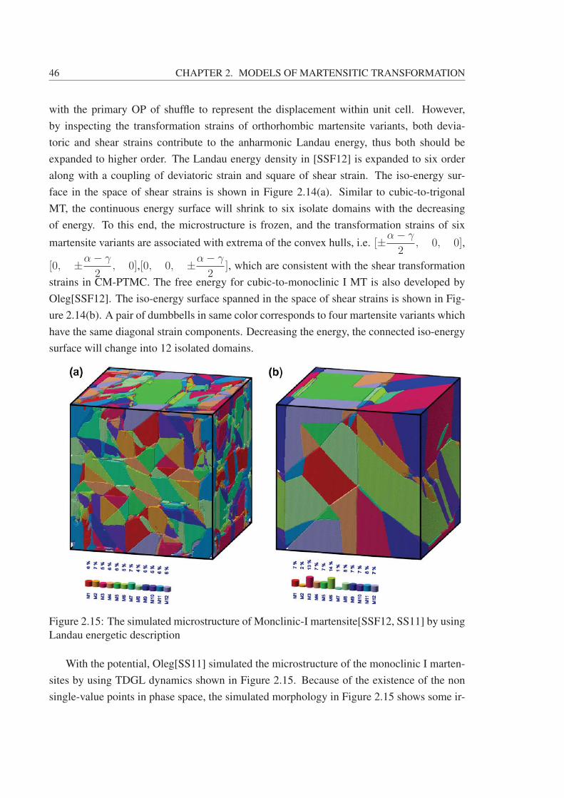
46 CHAPTER 2. MODELS OF MARTENSITIC TRANSFORMATION
with the primary OP of shuffle to represent the displacement within unit cell. However,
by inspecting the transformation strains of orthorhombic martensite variants, both devia-
toric and shear strains contribute to the anharmonic Landau energy, thus both should be
expanded to higher order. The Landau energy density in [SSF12] is expanded to six order
along with a coupling of deviatoric strain and square of shear strain. The iso-energy sur-
face in the space of shear strains is shown in Figure 2.14(a). Similar to cubic-to-trigonal
MT, the continuous energy surface will shrink to six isolate domains with the decreasing
of energy. To this end, the microstructure is frozen, and the transformation strains of six
martensite variants are associated with extrema of the convex hulls, i.e. [±α− γ
2, 0, 0],
[0, ±α− γ
2, 0],[0, 0, ±α− γ
2], which are consistent with the shear transformation
strains in CM-PTMC. The free energy for cubic-to-monoclinic I MT is also developed by
Oleg[SSF12]. The iso-energy surface spanned in the space of shear strains is shown in Fig-
ure 2.14(b). A pair of dumbbells in same color corresponds to four martensite variants which
have the same diagonal strain components. Decreasing the energy, the connected iso-energy
surface will change into 12 isolated domains.
Figure 2.15: The simulated microstructure of Monclinic-I martensite[SSF12, SS11] by using
Landau energetic description
With the potential, Oleg[SS11] simulated the microstructure of the monoclinic I marten-
sites by using TDGL dynamics shown in Figure 2.15. Because of the existence of the non
single-value points in phase space, the simulated morphology in Figure 2.15 shows some ir-
2.4. LANDAU THEORY WITH IRS 47
regular patterns incompatible with those in experiments and predicted by CM-PTMC. Thus,
the development of Landau models for cubic-to-orthorhombic and cubic-to-monoclinic MTs
is still far beyond closure.
2.4.11 Compatibility Kernel
The discovery of compatibility enforced long-range anisotropic kernel is no doubt a mile-
stone in the development of the nonlinear Landau model to understand the mechanisms be-
hind the formation of twin related microstructure in MTs. It provides a fundamental inter-
pretation of the preferential orientations observed in austenite and/or martensites. Detailed
in [LSR+03], the St. Venant’s compatibility condition connects non-OP strains with OP
strains, such that the non-OP harmonic energy yields an anisotropic long-range compatibil-
ity kernel with the OPs as independent variables. The minimum of this compatibility kernel,
which is the energy cost associated with the non-OP strains that the system tries to expel,
gives the domain boundary orientation. In the subsection, we revisit the compatibility ker-
nels of cubic-to-tetragonal and cubic-to-trigonal MTs, particularly, calculate the values of
compatibility kernel in directions and/or planes with the wave vector components ki = 0
The compatibility kernel is derived from the St. Venant’s compatibility. Since the true
independent variables to describe the deformation gradient in MT are the displacements, the
six symmetrized infinitesimal strain components are not independent. Thus, the St. Venant’s
compatibility can be expressed in strain tensor as
∇× (∇× e)T = 0 (in coordinate space)k× e(k)× k = 0 (in Fourier space)
(2.110)
in which, the incompatibility, defined as the double-Curl operation on strain, is vanishing for
a smooth compatible state. Eq. (2.110) can be expanded as two sets of three equations with
the independent variables of diagonal strain components,
2kykzε23 = k2yε33 + k2
zε222kxkzε13 = k2
xε33 + k2zε11
2kxkyε12 = k2xε22 + k2
yε11
(2.111)
or with the independent variables of off-diagonal strain components,
kykzε11 = −k2xε23 + kxkyε13 + kxkzε12
kxkzε22 = −k2yε13 + kykzε12 + kxkyε23
kxkyε33 = −k2zε12 + kxkzε23 + kykzε13
(2.112)
These equations yield the St. Venant’s constraints in terms of symmetry adapted strains in
Fourier space as
O(s)1 e1 + O
(s)2 e2 + O
(s)3 e3 + es=4,5,6 = 0 (2.113)
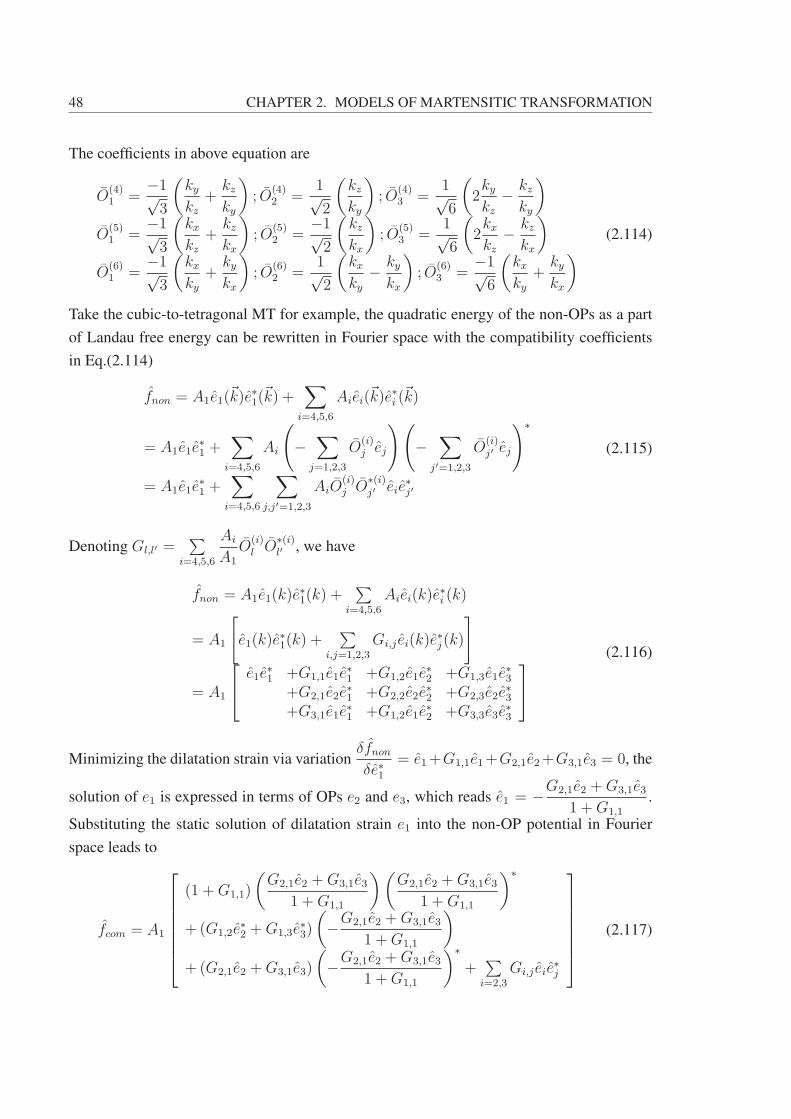
48 CHAPTER 2. MODELS OF MARTENSITIC TRANSFORMATION
The coefficients in above equation are
O(4)1 =
−1√3
(kykz
+kzky
); O
(4)2 =
1√2
(kzky
); O
(4)3 =
1√6
(2kykz
− kzky
)
O(5)1 =
−1√3
(kxkz
+kzkx
); O
(5)2 =
−1√2
(kzkx
); O
(5)3 =
1√6
(2kxkz
− kzkx
)
O(6)1 =
−1√3
(kxky
+kykx
); O
(6)2 =
1√2
(kxky
− kykx
); O
(6)3 =
−1√6
(kxky
+kykx
) (2.114)
Take the cubic-to-tetragonal MT for example, the quadratic energy of the non-OPs as a part
of Landau free energy can be rewritten in Fourier space with the compatibility coefficients
in Eq.(2.114)
fnon = A1e1(�k)e∗1(�k) +
∑i=4,5,6
Aiei(�k)e∗i (�k)
= A1e1e∗1 +
∑i=4,5,6
Ai
(−∑
j=1,2,3
O(i)j ej
)(−∑
j′=1,2,3
O(i)j′ ej
)∗
= A1e1e∗1 +
∑i=4,5,6
∑j,j′=1,2,3
AiO(i)j O
∗(i)j′ eie
∗j′
(2.115)
Denoting Gl,l′ =∑
i=4,5,6
Ai
A1
O(i)l O
∗(i)l′ , we have
fnon = A1e1(k)e∗1(k) +
∑i=4,5,6
Aiei(k)e∗i (k)
= A1
[e1(k)e
∗1(k) +
∑i,j=1,2,3
Gi,j ei(k)e∗j(k)
]
= A1
⎡⎣ e1e
∗1 +G1,1e1e
∗1 +G1,2e1e
∗2 +G1,3e1e
∗3
+G2,1e2e∗1 +G2,2e2e
∗2 +G2,3e2e
∗3
+G3,1e1e∗1 +G1,2e1e
∗2 +G3,3e3e
∗3
⎤⎦
(2.116)
Minimizing the dilatation strain via variationδfnonδe∗1
= e1+G1,1e1+G2,1e2+G3,1e3 = 0, the
solution of e1 is expressed in terms of OPs e2 and e3, which reads e1 = −G2,1e2 +G3,1e31 +G1,1
.
Substituting the static solution of dilatation strain e1 into the non-OP potential in Fourier
space leads to
fcom = A1
⎡⎢⎢⎢⎢⎢⎢⎣
(1 +G1,1)
(G2,1e2 +G3,1e3
1 +G1,1
)(G2,1e2 +G3,1e3
1 +G1,1
)∗
+(G1,2e∗2 +G1,3e
∗3)
(−G2,1e2 +G3,1e3
1 +G1,1
)
+(G2,1e2 +G3,1e3)
(−G2,1e2 +G3,1e3
1 +G1,1
)∗+∑i=2,3
Gi,j eie∗j
⎤⎥⎥⎥⎥⎥⎥⎦
(2.117)

2.4. LANDAU THEORY WITH IRS 49
Thus,
fcom =A1
(1 +G1,1)
[ − (G1,2e∗2 +G1,3e
∗3) (G2,1e2 +G3,1e3)
+∑i=2,3
Gi,j eie∗j +G1,1
∑i=2,3
Gi,j eie∗j
]
=A1
(1 +G1,1)
[ −G1,2G2,1e2e∗2 −G1,2G3,1e3e
∗2 −G1,3G2,1e2e
∗3 −G1,3G3,1e3e
∗3
+∑i=2,3
Gi,j eie∗j +G1,1
∑i=2,3
Gi,j eie∗j
]
=A1
(1 +G1,1)
∑i=2,3
[Gi,j + (Gi,jG1,1 −Gi,1Gj,1)]eie∗j
(2.118)
Finally, the static compatibility kernel for cubic-tetragonal MT is derived.
Ull′ =(1− δ(�k,0)
) Gi,j + (Gi,jG1,1 −Gi,1Gj,1)
(1 +G1,1)(2.119)
However, the values of the compatibility kernel at the special points in Fourier space,
where at least one of the wave vector components is equal to zero, should be carefully eval-
uated to ensure the smoothness of the compatibility kernel.
Now we take the case of kx �= 0, ky → 0, kz → 0 as example. Assuming ky = O (kz),
we have
O(4)1 =
−2√3; O
(4)2 =
1√2; O
(4)3 =
1√6
O(5)1 =
−1√3
kxkz
; O(5)2 = 0; O
(5)3 =
2√6
kxkz
O(6)1 =
−1√3
kxky
; O(6)2 =
1√2
kxky
; O(6)3 =
−1√6
kxky
(2.120)
G1,1 = O(4)1 O
(4)1 + O
(5)1 O
(5)1 + O
(6)1 O
(6)1 =
4
3+
1
3
(k2x
k2z
)+
1
3
(k2x
k2y
)
G2,2 = O(4)2 O
(4)2 + O
(5)2 O
(5)2 + O
(6)2 O
(6)2 =
1
2+ 0 +
1
2
(k2x
k2y
)
G3,3 = O(4)3 O
(4)3 + O
(5)3 O
(5)3 + O
(6)3 O
(6)3 =
1
6+
4
6
(k2x
k2z
)+
1
6
(k2x
k2y
)
G1,2 = O(4)1 O
(4)2 + O
(5)1 O
(5)2 + O
(6)1 O
(6)2 = − 2√
6+ 0 +
1√6
(k2x
k2y
)
G1,3 = O(4)1 O
(4)3 + O
(5)1 O
(5)3 + O
(6)1 O
(6)3 = − 2√
18− 2√
18
(k2x
k2z
)− 1√
18
(k2x
k2y
)
G2,3 = O(4)2 O
(4)3 + O
(5)2 O
(5)3 + O
(6)2 O
(6)3 =
1√12
− 1√12
(k2x
k2y
)
(2.121)

50 CHAPTER 2. MODELS OF MARTENSITIC TRANSFORMATION
U22 =G2,2 +G2,2G1,1 −G1,2G1,2
1 +G1,1
=
1
2
(1 +
k2x
k2y
)+
1
6
(1 +
k2x
k2y
)(4 +
k2x
k2z
+k2x
k2y
)− 1
6
(2− k2
x
k2y
)2
1 +4
3+
1
3
(k2x
k2z
)+
1
3
(k2x
k2y
)
=
3
(1 +
k2x
k2y
)+
(1 +
k2x
k2y
)(4 +
k2x
k2z
+k2x
k2y
)−(2− k2
x
k2y
)2
6 + 8 + 2
(k2xk
2y
k2z
)+ 2
(k2x
k2y
) ∼ k2x
2(k2y + k2
z
)
(2.122)
Provided ky(0) ≈ 1
Ny
, ky(0) ≈ 1
Ny
are used in numerical calculations, the minimum approx-
imate value of U22 along the direction is N2yN
2z k
2x/2(N2
y +N2z
). Similarly, we have derived
the expressions and values of compatibility kernel on other planes or along directions listed
in Appendix A as well as those for cubic-to-trigonal MT in Appendix B. With the compat-
ibility kernel, the preferential twinning orientation can be discerned, e.g. the ±π/4 in each
ki = 0 plane. It indicates the correspondence variant pair of cubic-to-tetragonal martensites
favors twinning orientation of ±π/4 on these planes.
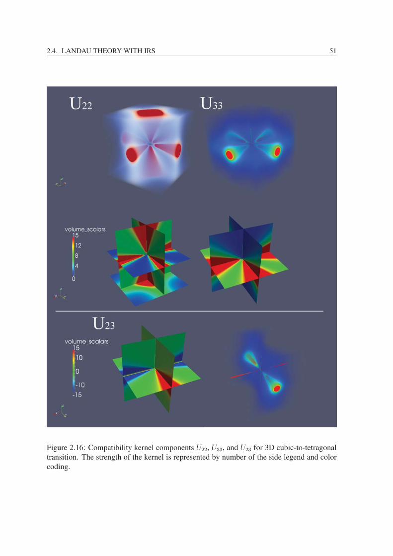
2.4. LANDAU THEORY WITH IRS 51
Figure 2.16: Compatibility kernel components U22, U33, and U23 for 3D cubic-to-tetragonal
transition. The strength of the kernel is represented by number of the side legend and color
coding.
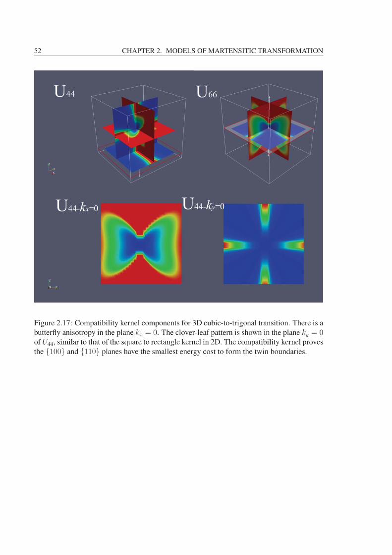
52 CHAPTER 2. MODELS OF MARTENSITIC TRANSFORMATION
Figure 2.17: Compatibility kernel components for 3D cubic-to-trigonal transition. There is a
butterfly anisotropy in the plane kx = 0. The clover-leaf pattern is shown in the plane ky = 0of U44, similar to that of the square to rectangle kernel in 2D. The compatibility kernel proves
the {100} and {110} planes have the smallest energy cost to form the twin boundaries.
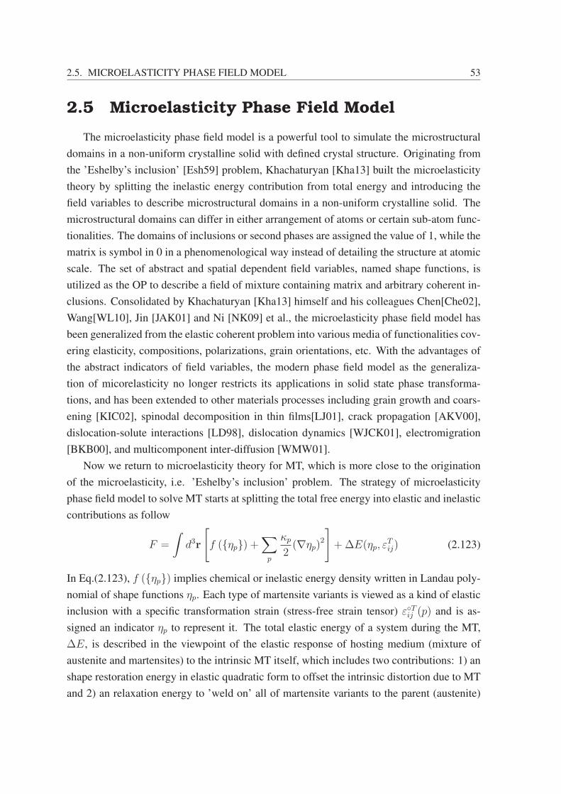
2.5. MICROELASTICITY PHASE FIELD MODEL 53
2.5 Microelasticity Phase Field Model
The microelasticity phase field model is a powerful tool to simulate the microstructural
domains in a non-uniform crystalline solid with defined crystal structure. Originating from
the ’Eshelby’s inclusion’ [Esh59] problem, Khachaturyan [Kha13] built the microelasticity
theory by splitting the inelastic energy contribution from total energy and introducing the
field variables to describe microstructural domains in a non-uniform crystalline solid. The
microstructural domains can differ in either arrangement of atoms or certain sub-atom func-
tionalities. The domains of inclusions or second phases are assigned the value of 1, while the
matrix is symbol in 0 in a phenomenological way instead of detailing the structure at atomic
scale. The set of abstract and spatial dependent field variables, named shape functions, is
utilized as the OP to describe a field of mixture containing matrix and arbitrary coherent in-
clusions. Consolidated by Khachaturyan [Kha13] himself and his colleagues Chen[Che02],
Wang[WL10], Jin [JAK01] and Ni [NK09] et al., the microelasticity phase field model has
been generalized from the elastic coherent problem into various media of functionalities cov-
ering elasticity, compositions, polarizations, grain orientations, etc. With the advantages of
the abstract indicators of field variables, the modern phase field model as the generaliza-
tion of micorelasticity no longer restricts its applications in solid state phase transforma-
tions, and has been extended to other materials processes including grain growth and coars-
ening [KIC02], spinodal decomposition in thin films[LJ01], crack propagation [AKV00],
dislocation-solute interactions [LD98], dislocation dynamics [WJCK01], electromigration
[BKB00], and multicomponent inter-diffusion [WMW01].
Now we return to microelasticity theory for MT, which is more close to the origination
of the microelasticity, i.e. ’Eshelby’s inclusion’ problem. The strategy of microelasticity
phase field model to solve MT starts at splitting the total free energy into elastic and inelastic
contributions as follow
F =
∫d3r
[f ({ηp}) +
∑p
κp
2(∇ηp)
2
]+ΔE(ηp, ε
Tij) (2.123)
In Eq.(2.123), f ({ηp}) implies chemical or inelastic energy density written in Landau poly-
nomial of shape functions ηp. Each type of martensite variants is viewed as a kind of elastic
inclusion with a specific transformation strain (stress-free strain tensor) ε◦Tij (p) and is as-
signed an indicator ηp to represent it. The total elastic energy of a system during the MT,
ΔE, is described in the viewpoint of the elastic response of hosting medium (mixture of
austenite and martensites) to the intrinsic MT itself, which includes two contributions: 1) an
shape restoration energy in elastic quadratic form to offset the intrinsic distortion due to MT
and 2) an relaxation energy to ’weld on’ all of martensite variants to the parent (austenite)
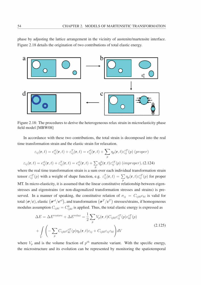
54 CHAPTER 2. MODELS OF MARTENSITIC TRANSFORMATION
phase by adjusting the lattice arrangement in the vicinity of austenite/martensite interface.
Figure 2.18 details the origination of two contributions of total elastic energy.
Figure 2.18: The procedures to derive the heterogeneous relax strain in microelasticity phase
field model [MBW08]
In accordance with these two contributions, the total strain is decomposed into the real
time transformation strain and the elastic strain for relaxation.
εij(r, t) = eelij(r, t) + εTij(r, t) = eelij(r, t) +∑p
ηp(r, t)ε◦Tij (p) (proper)
εij(r, t) = eelij(r, t) + εTij(r, t) = eelij(r, t) +∑p
η2p(r, t)ε◦Tij (p) (improper), (2.124)
where the real time transformation strain is a sum over each individual transformation strain
tensor ε◦Tij (p) with a weight of shape function, e.g. εTij(r, t) =∑p
ηp(r, t)ε◦Tij (p) for proper
MT. In micro-elasticity, it is assumed that the linear constitutive relationship between eigen-
stresses and eigenstrains (or non-diagonalized transformation stresses and strains) is pre-
served. In a manner of speaking, the constitutive relation of σij = Cijklekl is valid for
total (σ/ε), elastic(σel/eel
), and transformation
(σT/εT
)stresses/strains, if homogeneous
modulus assumption Cijkl = C0ijkl is applied. Thus, the total elastic energy is expressed as
ΔE = ΔErestore +ΔErelax =1
2
∑p
Vp(r, t)Cijklε◦Tij (p)ε
◦Tkl (p)
+
∫V
(−∑p
Cijklε◦Tkl (p)ηp(r, t)εij + Cijklεijεkl
)dV
(2.125)
where Vp and is the volume fraction of pth martensite variant. With the specific energy,
the microstructure and its evolution can be represented by monitoring the spatiotemporal
2.5. MICROELASTICITY PHASE FIELD MODEL 55
evolution of ηp under a quasi-equilibrium condition, assuming that the elastic equilibrium
state is achieved instantly at each time step. Therefore, there are actually one kinetic equation
and one static equation. The kinetic equation is the well-known Allen-Cahn equation to
record the evolution of OPs ηp
∂ηp(r, t)
∂t= −Lp
δF
δηp(r, t)+ ξp(r, t) (2.126)
where Lp is kinetic coefficient and ξp is Langevin random force term of thermal fluctuation.
The static one is a variational minimization of the relaxation energy with respect to the
displacement under certain boundary conditions to attain the elastic equilibrium state.
δΔErelax
δu= 0 (2.127)
Since all parts in total elastic energy are formally quadratic and the total strain is the sym-
metric part of the displacement derivatives to space by applying infinitesimal approximation
εij(r, t) =1
2
(∂ui(r, t)
∂xj
+∂uj(r, t)
∂xi
)(2.128)
the variation in Eq(2.127) can be equivalently transformed into the mechanical equilibrium
equation,
∂σij
∂xj
=Cijkl∂σkl
∂xj
= 0
∂
∂xj
Cijkl1
2
(∂uk(r, t)
∂xl
+∂ul(r, t)
∂xk
)=
∂
∂xj
CijklεTij(r, t)
(2.129)
However, an analytical solution of Eq.(2.129) in Fourier space requires a homogeneous
boundary condition that displacement u and displacement gradient ∇u do vanish at external
surfaces. These conditions can be valid when displacement and total strain are divided into
homogeneous (u, εij) and heterogeneous (�u, δεij) parts, viz.
u(r) = u+�u(r), εij(r) = εij + δεij(r) (2.130)
In this formalism, the homogeneous strain εij describes the spatial independent, uniform
shape deformation of a crystal. While, the spatial varying heterogeneous strain is written as
the symmetric part of local displacement gradient in infinitesimal approximation
δεij(r, t) =1
2
(∂�ui(r, t)
∂xj
+∂�uj(r, t)
∂xi
)(2.131)

56 CHAPTER 2. MODELS OF MARTENSITIC TRANSFORMATION
The homogeneous strain together with heterogeneous strain strain leads to the total strain
satisfying
∫drδεij(r) ≡ 0 (2.132)
Representing the equation δΔErelax/δ�u = 0 in Fourier space, i.e.
−kjklCijkl�uk(k, t) = ikjCijklεTij(k, t) (2.133)
leads to an explicit solution of local displacement
�uk(k, t) = −ik−2Ω0ik (n)kjσ
Tij(k, t) (2.134)
where σTij(k, t) = Cijkl
[∑p
ηp(r, t)ε◦Tij (p)
]F
, [Ω0ik]
−1(n) = Cijklnjnl and n = k/|k|.
Substituting the solution (2.134) into Eqs.(2.124, 2.130), the expressions of total strain and
elastic strain are obtained.
εij(r) = εij +1
2F−1
{[njΩ
0ki (n) + niΩ
0kj (n)
]njσ
Tkl(k, t)
}eelij(r) = εij +
1
2F−1
{[njΩ
0ki (n) + niΩ
0kj (n)
]njσ
Tkl(k, t)
}− εTij(r, t)(2.135)
as well as the updated total elastic energy
ΔE =1
2
∫Cijkle
elije
elkldr
3
=1
2
∫Cijklε
Tij(r, t)ε
Tkl(r, t)dr
3 +V
2Cijklεij εkl − εij
∫Cijklε
Tkl(r, t)dr
3
−1
2
◦∫d3k
(2π)3[niσ
Tij(k, t)Ω
0jk (n) σ
Tkl(k, t)nj
]
=1
2
∑p,q
◦∫d3k
(2π)3Bpqηp(k, t)η
∗q (k, t)
(2.136)
where, F and F−1 denote the Fourier and inverse Fourier transformations;
◦∫is the integral
without the point k = 0. Bpq =
{Cijklε
◦Tij (p)ε
◦Tkl (q) (n = 0)
Cijklε◦Tij (p)ε
◦Tkl (q)− niσ
Tij(p)Ω
0jkσ
Tkl(q)nj (n �= 0)
.
The new shape function satisfies
∫d3k
(2π)3ηp(k, t)η
∗q (k, t) = δpqVp − VpVq
V. V is the total
volume fraction of all martensites. So far, the elastic energy density is the sum over the prod-
uct of the materials dependent kernel Bpq and the spatiotemporal dependent shape functions
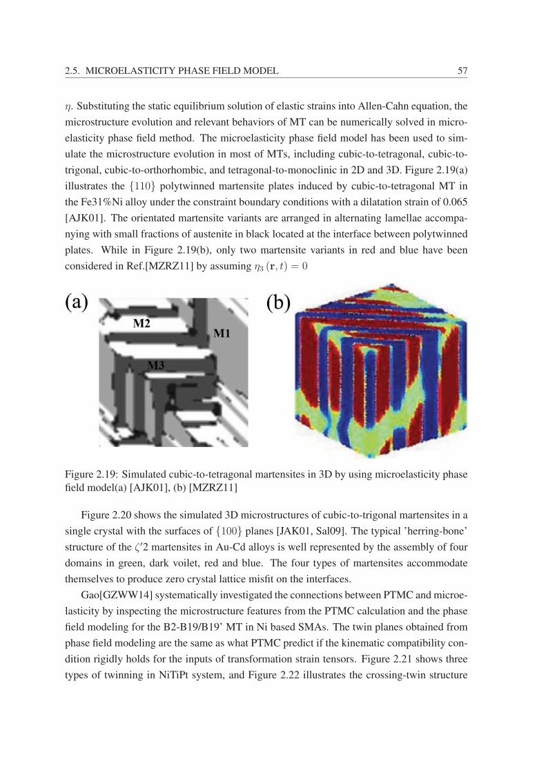
2.5. MICROELASTICITY PHASE FIELD MODEL 57
η. Substituting the static equilibrium solution of elastic strains into Allen-Cahn equation, the
microstructure evolution and relevant behaviors of MT can be numerically solved in micro-
elasticity phase field method. The microelasticity phase field model has been used to sim-
ulate the microstructure evolution in most of MTs, including cubic-to-tetragonal, cubic-to-
trigonal, cubic-to-orthorhombic, and tetragonal-to-monoclinic in 2D and 3D. Figure 2.19(a)
illustrates the {110} polytwinned martensite plates induced by cubic-to-tetragonal MT in
the Fe31%Ni alloy under the constraint boundary conditions with a dilatation strain of 0.065
[AJK01]. The orientated martensite variants are arranged in alternating lamellae accompa-
nying with small fractions of austenite in black located at the interface between polytwinned
plates. While in Figure 2.19(b), only two martensite variants in red and blue have been
considered in Ref.[MZRZ11] by assuming η3 (r, t) = 0
Figure 2.19: Simulated cubic-to-tetragonal martensites in 3D by using microelasticity phase
field model(a) [AJK01], (b) [MZRZ11]
Figure 2.20 shows the simulated 3D microstructures of cubic-to-trigonal martensites in a
single crystal with the surfaces of {100} planes [JAK01, Sal09]. The typical ’herring-bone’
structure of the ζ ′2 martensites in Au-Cd alloys is well represented by the assembly of four
domains in green, dark voilet, red and blue. The four types of martensites accommodate
themselves to produce zero crystal lattice misfit on the interfaces.
Gao[GZWW14] systematically investigated the connections between PTMC and microe-
lasticity by inspecting the microstructure features from the PTMC calculation and the phase
field modeling for the B2-B19/B19’ MT in Ni based SMAs. The twin planes obtained from
phase field modeling are the same as what PTMC predict if the kinematic compatibility con-
dition rigidly holds for the inputs of transformation strain tensors. Figure 2.21 shows three
types of twinning in NiTiPt system, and Figure 2.22 illustrates the crossing-twin structure
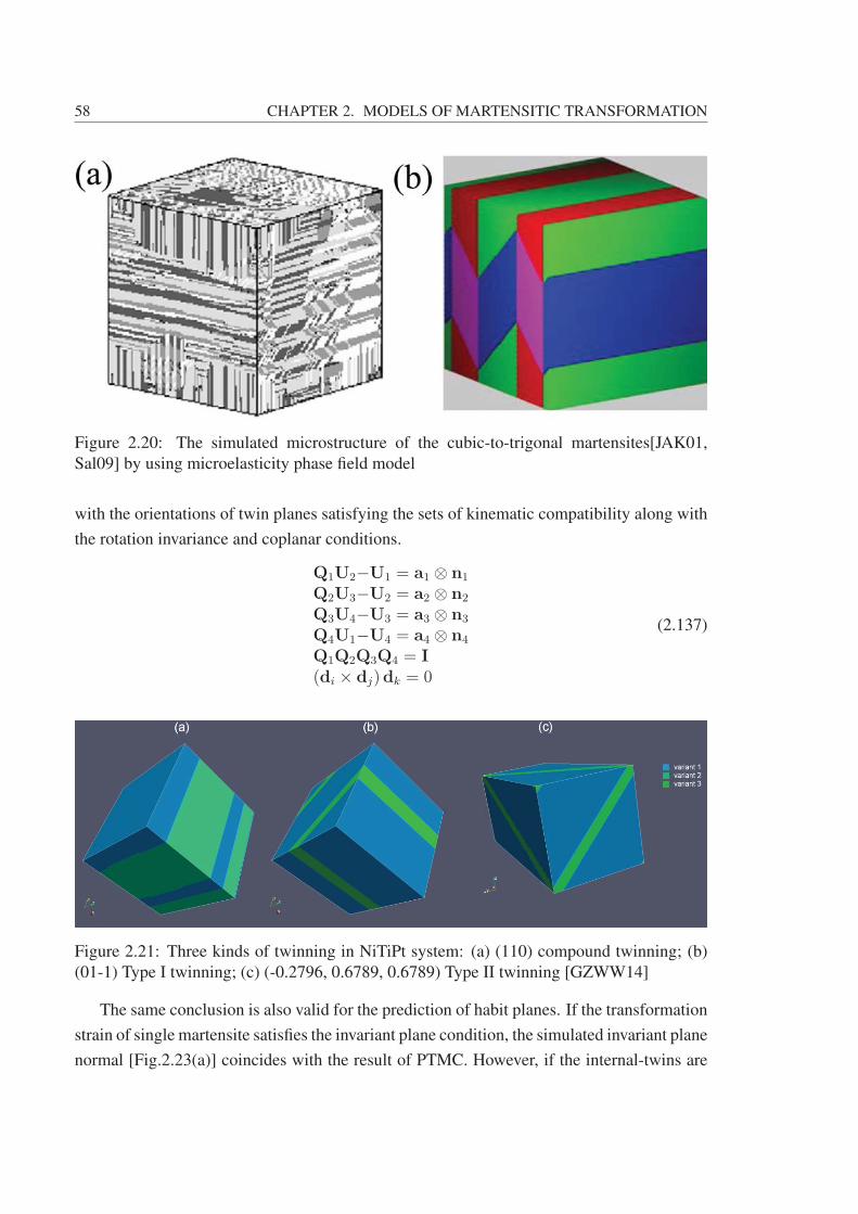
58 CHAPTER 2. MODELS OF MARTENSITIC TRANSFORMATION
Figure 2.20: The simulated microstructure of the cubic-to-trigonal martensites[JAK01,
Sal09] by using microelasticity phase field model
with the orientations of twin planes satisfying the sets of kinematic compatibility along with
the rotation invariance and coplanar conditions.
Q1U2−U1 = a1 ⊗ n1
Q2U3−U2 = a2 ⊗ n2
Q3U4−U3 = a3 ⊗ n3
Q4U1−U4 = a4 ⊗ n4
Q1Q2Q3Q4 = I(di × dj)dk = 0
(2.137)
Figure 2.21: Three kinds of twinning in NiTiPt system: (a) (110) compound twinning; (b)
(01-1) Type I twinning; (c) (-0.2796, 0.6789, 0.6789) Type II twinning [GZWW14]
The same conclusion is also valid for the prediction of habit planes. If the transformation
strain of single martensite satisfies the invariant plane condition, the simulated invariant plane
normal [Fig.2.23(a)] coincides with the result of PTMC. However, if the internal-twins are
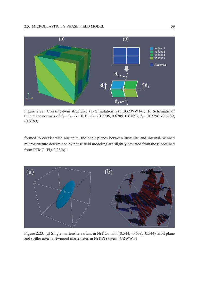
2.5. MICROELASTICITY PHASE FIELD MODEL 59
Figure 2.22: Crossing-twin structure: (a) Simulation result[GZWW14]; (b) Schematic of
twin plane normals of d1= d3= (-1, 0, 0), d2= (0.2796, 0.6789, 0.6789), d4= (0.2796, -0.6789,
-0.6789)
formed to coexist with austenite, the habit planes between austenite and internal-twinned
microstructure determined by phase field modeling are slightly deviated from those obtained
from PTMC [Fig.2.23(b)].
Figure 2.23: (a) Single martensite variant in NiTiCu with (0.544, -0.638, -0.544) habit plane
and (b)the internal-twinned martensites in NiTiPt system [GZWW14]

60 CHAPTER 2. MODELS OF MARTENSITIC TRANSFORMATION
2.6 Thermomechanical Phase Field Model
In sections 2.3 and 2.4, the IRS-Landau and microelasticity phase field models have
been advanced as powerful tools to represent and predict fine martensitic microstructure.
However, these works are insufficient to represent some of mechanical properties of SMAs
such as weakly temperature dependent stress hysteresis, and nonzero tangent elastic mod-
uli at the phase transformation point. In microelasticity, the Landau free energy used in
[WK97, MZEKC13], predicts the total transformation strain varying with direct and inverse
transformations. The IRS based Landau potential[Fal83] predicts stress hysteresis changing
with temperatures, in contrast with the typical stress-strain curves of SMA exhibit a constant
transformation strain and stress hysteresis at different temperatures[LP02]. Therefore, Levi-
tas and Lee [LPL03] developed thermomechanical phase field model incorporating elasticity
and Landau energetics for the multivariant stress- and temperature- induced MTs, which can
correctly describe the aforementioned mechanical features of SMAs. In thermomechanical
model, the total strain tensor ε is also decomposed into the elastic εel and transformation
εtkϕ (a, ηk) parts, i.e.
ε = εel + εtkϕ (a, ηk) (2.138)
where εtk is the transformation strain tensor of kth martensite variant at thermodynamic
equilibrium state, and k = 0 corresponds to austenite. Such that, the Gibbs energy density is
expressed as
G = −1
2σ : S : σ + σ :εt +
n−1∑i=1
n∑j=i+1
Hij (ηi, ηj) (2.139)
εt =n∑
k=1
εtk[a
2η2k + (3− a) η4k +
1
2(a− 4) η6k
]−
n−1∑i=1
n∑j=i+1
η2i η2j
(η2iDij + η2jDji
)(2.140)
Dij =1
2(a− 3) εtj +
3
2εti (2.141)
Hij (ηi, ηj) = Bη2i η2j +
(A
2− A
2− B
)η4i η
2j +C|ηi|3|ηj|3+
(A
2− A
2−B
)η2i η
4j (2.142)
A = A0 (T − Tc) (2.143)
Here,ηk is the OP (0 < ηk < 1). σ : ε = σijεij are the contraction of tensors over one and
two indices, σ is stress tensor, S is forth-rank elastic compliance tensor. Tc, a, A0, B, and C
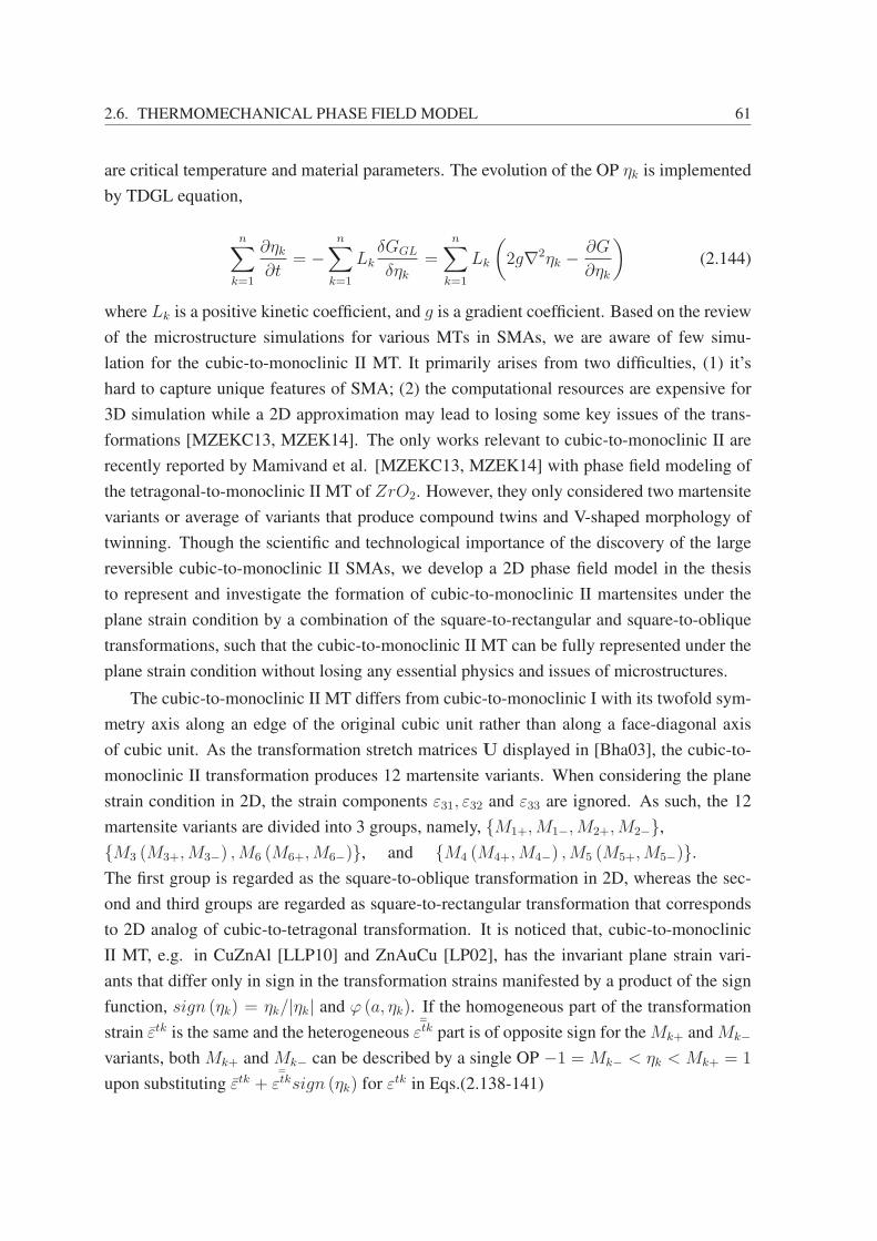
2.6. THERMOMECHANICAL PHASE FIELD MODEL 61
are critical temperature and material parameters. The evolution of the OP ηk is implemented
by TDGL equation,
n∑k=1
∂ηk∂t
= −n∑
k=1
LkδGGL
δηk=
n∑k=1
Lk
(2g∇2ηk − ∂G
∂ηk
)(2.144)
where Lk is a positive kinetic coefficient, and g is a gradient coefficient. Based on the review
of the microstructure simulations for various MTs in SMAs, we are aware of few simu-
lation for the cubic-to-monoclinic II MT. It primarily arises from two difficulties, (1) it’s
hard to capture unique features of SMA; (2) the computational resources are expensive for
3D simulation while a 2D approximation may lead to losing some key issues of the trans-
formations [MZEKC13, MZEK14]. The only works relevant to cubic-to-monoclinic II are
recently reported by Mamivand et al. [MZEKC13, MZEK14] with phase field modeling of
the tetragonal-to-monoclinic II MT of ZrO2. However, they only considered two martensite
variants or average of variants that produce compound twins and V-shaped morphology of
twinning. Though the scientific and technological importance of the discovery of the large
reversible cubic-to-monoclinic II SMAs, we develop a 2D phase field model in the thesis
to represent and investigate the formation of cubic-to-monoclinic II martensites under the
plane strain condition by a combination of the square-to-rectangular and square-to-oblique
transformations, such that the cubic-to-monoclinic II MT can be fully represented under the
plane strain condition without losing any essential physics and issues of microstructures.
The cubic-to-monoclinic II MT differs from cubic-to-monoclinic I with its twofold sym-
metry axis along an edge of the original cubic unit rather than along a face-diagonal axis
of cubic unit. As the transformation stretch matrices U displayed in [Bha03], the cubic-to-
monoclinic II transformation produces 12 martensite variants. When considering the plane
strain condition in 2D, the strain components ε31, ε32 and ε33 are ignored. As such, the 12
martensite variants are divided into 3 groups, namely, {M1+,M1−,M2+,M2−},
{M3 (M3+,M3−) ,M6 (M6+,M6−)}, and {M4 (M4+,M4−) ,M5 (M5+,M5−)}.
The first group is regarded as the square-to-oblique transformation in 2D, whereas the sec-
ond and third groups are regarded as square-to-rectangular transformation that corresponds
to 2D analog of cubic-to-tetragonal transformation. It is noticed that, cubic-to-monoclinic
II MT, e.g. in CuZnAl [LLP10] and ZnAuCu [LP02], has the invariant plane strain vari-
ants that differ only in sign in the transformation strains manifested by a product of the sign
function, sign (ηk) = ηk/|ηk| and ϕ (a, ηk). If the homogeneous part of the transformation
strain εtk is the same and the heterogeneous¯εtk part is of opposite sign for the Mk+ and Mk−
variants, both Mk+ and Mk− can be described by a single OP −1 = Mk− < ηk < Mk+ = 1
upon substituting εtk +¯εtksign (ηk) for εtk in Eqs.(2.138-141)
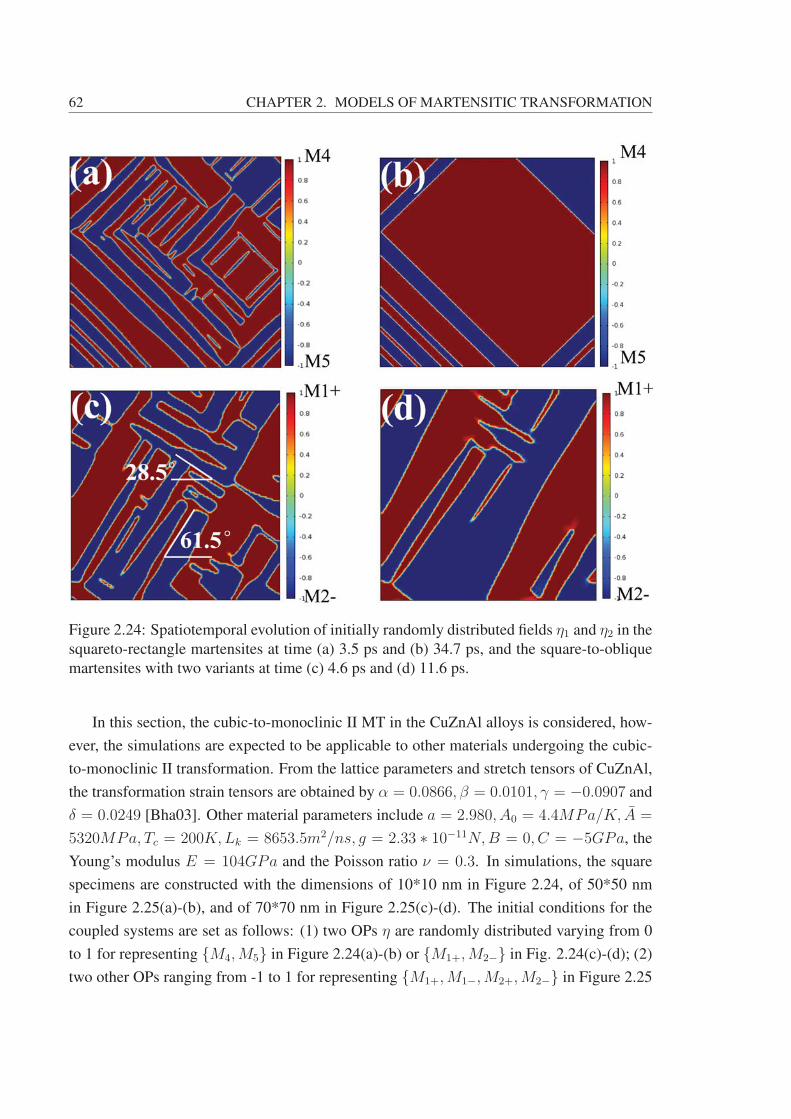
62 CHAPTER 2. MODELS OF MARTENSITIC TRANSFORMATION
Figure 2.24: Spatiotemporal evolution of initially randomly distributed fields η1 and η2 in the
squareto-rectangle martensites at time (a) 3.5 ps and (b) 34.7 ps, and the square-to-oblique
martensites with two variants at time (c) 4.6 ps and (d) 11.6 ps.
In this section, the cubic-to-monoclinic II MT in the CuZnAl alloys is considered, how-
ever, the simulations are expected to be applicable to other materials undergoing the cubic-
to-monoclinic II transformation. From the lattice parameters and stretch tensors of CuZnAl,
the transformation strain tensors are obtained by α = 0.0866, β = 0.0101, γ = −0.0907 and
δ = 0.0249 [Bha03]. Other material parameters include a = 2.980, A0 = 4.4MPa/K, A =
5320MPa, Tc = 200K,Lk = 8653.5m2/ns, g = 2.33 ∗ 10−11N,B = 0, C = −5GPa, the
Young’s modulus E = 104GPa and the Poisson ratio ν = 0.3. In simulations, the square
specimens are constructed with the dimensions of 10*10 nm in Figure 2.24, of 50*50 nm
in Figure 2.25(a)-(b), and of 70*70 nm in Figure 2.25(c)-(d). The initial conditions for the
coupled systems are set as follows: (1) two OPs η are randomly distributed varying from 0
to 1 for representing {M4,M5} in Figure 2.24(a)-(b) or {M1+,M2−} in Fig. 2.24(c)-(d); (2)
two other OPs ranging from -1 to 1 for representing {M1+,M1−,M2+,M2−} in Figure 2.25

2.6. THERMOMECHANICAL PHASE FIELD MODEL 63
are randomly seeded in the whole specimens.
Figure 2.24(a)-(b) show the characteristic (a) needle and (b) lamellar twins of the square-
to-rectangular martensites as analog of the cubic-to-monoclinic II ones, wherein the observed
interface directions of ±45◦ are formed at transient state resulted from kinematic compat-
ibility condition, while the martensite variant coalescence is promoted by the surface en-
ergy in the later stage. It should be stressed that the compound twins, such as {M4,M5}or {M3,M6} obtained from the square-to-rectangular transformation and {M1+,M2+} or
{M1−,M2−} from the square-to-oblique transformation, have the ±45◦ direction angles of
twin planes, which are originating from the difference between the diagonal components in
the transformation strain. As one may expect, the twinning directions of the correspondence
variant pairs of {M1+,M2−} and {M1−,M2+} deviate from ±45◦ and 0◦ or 90◦. Figure
2.24(c)-(d) show the laths/needles aligning along the ±61.5◦ or ∓28.5◦ due to the difference
between the diagonal and shear components in the transformation strains. Figure 2.25(a)-(b)
show the richness of the intricate microstructures of the square-to-oblique transformation as
analog of the different cubic-to-monoclinic II alloys, including polygons like triangle, trape-
zoid and hexagon, which may occur under different experimental conditions. The twins of
{M1+,M2−} and {M1−,M2+} have the ±61.5◦ or ∓28.5◦ directions of twin planes, thus
lead to the polygon morphology. Increasing the specimen dimension, Fig. 2.25(c)-(d) pre-
dict the V-tapered accommodated microstructures observed in the CuZnAl alloys by Zhang
et al. [ZZZ99] (see the inset of Figure 2.25(d)). Similar to the classic wedge microstruc-
tures, the V-shaped twins play a major role in the initiation and growth of MT, which might
in turn governing direct and reverse MTs. Note that, another possible compound twins,
e.g. {M1+,M1−} and {M2+,M2−} embracing 0◦ or 90◦ interface directions with lamellar
microstructure are not observed in our simulations, but they are allowed according to the
kinematic compatibility.
The simulated martensite microstructure also can be verified with the CM-PTMC by us-
ing the Eqs.(2.45-58) in Section 2.3 and Ref.[Bha03]. When κ12 = ±1 and ρ �= 0 are chosen
to make |n| = 1, from Eq. (2.51), we obtain the twin plane normal [±1, 0, 0] or [0,±1, 0] per-
pendicular to the interface between M1+ and M1− (or M2+ and M2−),[±1/√
2,∓ 1/√
2,0]
or[±1/√
2,± 1/√
2,0]
to the one between M1+ and M2+ (M1− and M2−, M3 and M6, or
M4 and M5), and [∓0.476673,± 0.879081, 0] or [±0.879081,± 0.476673,0] to one between
M1+ and M2− (M1− and M2+). All the simulated twin plane normals in Figures 2.24 and
2.25 exactly coincide with these calculated results based on Eq. (2.53).
From the thermodynamic equilibrium conditions, see Eqs. (14) and (16) in Ref.[LLP10],
the parametric representation of the unstable branch of equilibrium stress-strain curves can
be obtained. They characterize the mechanical behaviors of cubic-to-monoclinic II SMAs at

64 CHAPTER 2. MODELS OF MARTENSITIC TRANSFORMATION
Figure 2.25: Spatiotemporal evolution of initially randomly distributed fields η1 +2η2 in the
square-to-oblique martensites at time (a) 40.4 ps and (b) 347 ps with the size of 50*50 nm,
and (c)80.9 ps and (d) 347 ps with the size of 70*70 nm. The V-shaped pattern is compared
with experiment [ZZZ99]
various temperatures (Figure 2.26). The A → M(M → A) transformation takes place at
higher (lower) stress in each hysteresis. The stress-strain curve at equilibrium temperature, =
300K, is termed ’pseudoplasticity’, while at higher temperatures is ’pseudoelasticity’; both
curves resemble that of a SMA.
2.7 Connections and Distinctions among Mod-els
In the previous Sections 2.2-2.5, we highlighted the widely used models of MT which
have ability to present/predict the intriguing microstructural features. These models have
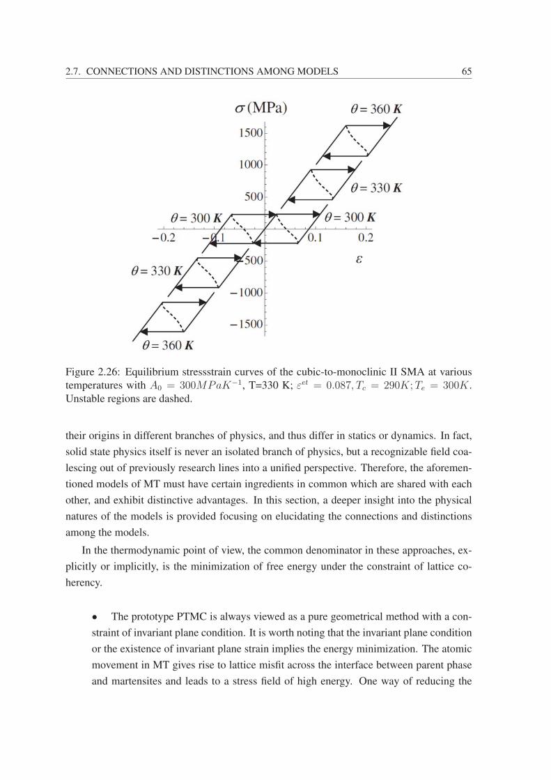
2.7. CONNECTIONS AND DISTINCTIONS AMONG MODELS 65
Figure 2.26: Equilibrium stressstrain curves of the cubic-to-monoclinic II SMA at various
temperatures with A0 = 300MPaK−1, T=330 K; εet = 0.087, Tc = 290K;Te = 300K.
Unstable regions are dashed.
their origins in different branches of physics, and thus differ in statics or dynamics. In fact,
solid state physics itself is never an isolated branch of physics, but a recognizable field coa-
lescing out of previously research lines into a unified perspective. Therefore, the aforemen-
tioned models of MT must have certain ingredients in common which are shared with each
other, and exhibit distinctive advantages. In this section, a deeper insight into the physical
natures of the models is provided focusing on elucidating the connections and distinctions
among the models.
In the thermodynamic point of view, the common denominator in these approaches, ex-
plicitly or implicitly, is the minimization of free energy under the constraint of lattice co-
herency.
• The prototype PTMC is always viewed as a pure geometrical method with a con-
straint of invariant plane condition. It is worth noting that the invariant plane condition
or the existence of invariant plane strain implies the energy minimization. The atomic
movement in MT gives rise to lattice misfit across the interface between parent phase
and martensites and leads to a stress field of high energy. One way of reducing the
66 CHAPTER 2. MODELS OF MARTENSITIC TRANSFORMATION
stress is to create up an incoherent interface. It has never been adopted by most of
SMAs to solve the problem since the phase transition proceeds by rapid interface mo-
tion that only allows coherent interfaces. Thus, the formation of coherent interface
with invariant plane strain is the exclusive way for SMAs to vanish lattice misfit stress.
Moreover, the lattice correspondence served as a priori discipline in fact corresponds
to the minimum transformation energy, which is determined by an ergodic comparison
of energy costs of displacing the lattice directions of parent phase to martensites.
The feature of energy minimization is apparent in the remaining models.
• The CM-PTMC approach minimizes a nonconvex harmonic elastic energy in
terms of the deformation gradient subject to the kinematic compatibility (Hadamard
jump) condition across the interface. The invariant plane strain condition in prototype
PTMC is one of special cases of kinematic compatibility condition.
• In microelasticity phase field model [Kha13], the total strain is written as the sum-
mation of transformation strains and elastic strain. The elastic free energy is harmonic
with respect to the elastic strain, which is effectively eliminated by using the static
equilibrium equation of elastic stress. Thus, the microelasticity phase field model
minimizes a transformation strain energy in terms of OPs η instead of total strains.
Nevertheless, the OP η in phase field modeling for MT is actually coupled to the trans-
formation strain. It should be noted that while the growth of the martensite is mostly
driven by the chemical free energy, the refining and coalescence of the microstructure
are driven by the strain energy and the interfacial energy reduction in microelasticity.
• The IRS based Landau model is equipped with the multi-well Landau free energy
in terms of symmetry adapted strains, which are linked with components of transfor-
mation strain tenors and displacements. To this sense, IRS-Landau model minimizes
an anharmonic strain energy, which drives structural transformations from higher sym-
metry to lower one. However, IRS based Landau energetics with different dynamics
exhibit different ways to achieve the minima of the transformation strain energy.
In dynamics,
• two PTMC methods depict the static microstructure features either obtained from
stress equilibrium or as variational result of elastic energy with respect to the defor-
mation gradient/strain components. Since the PTMC methods only involve the elastic
energy density, neither coordinate variables nor time dependent dynamics is taken into
models, they are incompetent to represent the morphology under TEM observation and
hence incapable of monitoring the evolution of microstructure with time. By the end,
the calculated habit planes and twin domain walls in statics only have geometric ex-
2.7. CONNECTIONS AND DISTINCTIONS AMONG MODELS 67
pressions in crystallography.
• The microelasticity and thermomechanical phase field models consider a split dy-
namics. The elastic strain reaches equilibrium state instantly, however, the transfor-
mation strains represented by OPs ηi are evolving with overdamped TDGL dynamics.
Thus, the rate of evolution (by tracking the local value of the OP η in a given region of
phase space) is proportional to the thermodynamic driving force, such that the elastic
system simply follows the gradient of the energy surface until it ends up in a local
minimum. The TDGL dynamics applied to the constructed free energy enables het-
erogeneous microstructure of martensite, but some of the dynamic behaviors such as
dynamical twinning, precursors will be missing. It is particularly suitable for steels and
other systems in which MTs undergo classical transformation paths with remarkable
dissipation originating from evolution of dislocation and friction of interface motion.
• The IRS based Landau approach is flexible to various dynamics, including static
equilibrium of stress, full dissipative overdamped, TDGL, and inertia ones. The iner-
tia dynamics can be performed using either displacements or stains as basic variables
in simulation. The displacement-based inertia dynamics (Lagrange dynamics in the
thesis) utilizes the general equation of motion, which is adopted in most of the simu-
lations in following chapters. The strain-based inertia dynamics [denominated Bales-
Gooding (BG) dynamics] requires the St. Venant’s compatibility constraint to serve as
the Lagrangian multiplier and the elimination of the dependent strain components by
rewriting the non-OP strains in terms of the OP strains, which results in an anisotropic,
long-range integral kernel of OP strains. (detailed in 2.4.11) The compatibility en-
forces the continuity across the interface and guarantees strain matching [LSR+03]. If
the dissipation (real damping) term is removed, the conservation equation of inertia dy-
namics describes a physical picture that the reduction in local free energy triggers the
formation of the habit planes and/or twin boundaries during the martensitic nucleation
and drives the interface propagation during martensite growth. In fact, the existence of
dissipation term will minimize the finite kinetic energy density. Finally, damping term
dissipates the energy to the state of stress equilibrium, which corresponds to an energy
minimum.
The inertia dynamics has ability to present a full physical picture of MT, including con-
version of Landau potential energy and kinetic energy, finite velocity of interface propagation
(inertial effect), dissipation of the excess energy due to friction, etc., such that the equations
of inertia dynamics in fact contain all of the essential elements of other dynamics. If both
inertia and viscous terms are dropped, the dynamic equation degenerates into the static equi-
librium of stress utilized in CM-PTMC, by doing so the static martensitic microstructure will
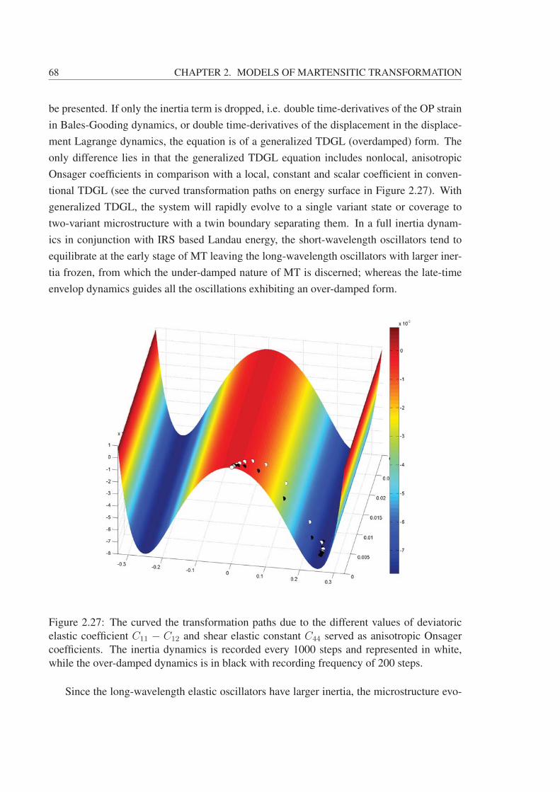
68 CHAPTER 2. MODELS OF MARTENSITIC TRANSFORMATION
be presented. If only the inertia term is dropped, i.e. double time-derivatives of the OP strain
in Bales-Gooding dynamics, or double time-derivatives of the displacement in the displace-
ment Lagrange dynamics, the equation is of a generalized TDGL (overdamped) form. The
only difference lies in that the generalized TDGL equation includes nonlocal, anisotropic
Onsager coefficients in comparison with a local, constant and scalar coefficient in conven-
tional TDGL (see the curved transformation paths on energy surface in Figure 2.27). With
generalized TDGL, the system will rapidly evolve to a single variant state or coverage to
two-variant microstructure with a twin boundary separating them. In a full inertia dynam-
ics in conjunction with IRS based Landau energy, the short-wavelength oscillators tend to
equilibrate at the early stage of MT leaving the long-wavelength oscillators with larger iner-
tia frozen, from which the under-damped nature of MT is discerned; whereas the late-time
envelop dynamics guides all the oscillations exhibiting an over-damped form.
Figure 2.27: The curved the transformation paths due to the different values of deviatoric
elastic coefficient C11 − C12 and shear elastic constant C44 served as anisotropic Onsager
coefficients. The inertia dynamics is recorded every 1000 steps and represented in white,
while the over-damped dynamics is in black with recording frequency of 200 steps.
Since the long-wavelength elastic oscillators have larger inertia, the microstructure evo-
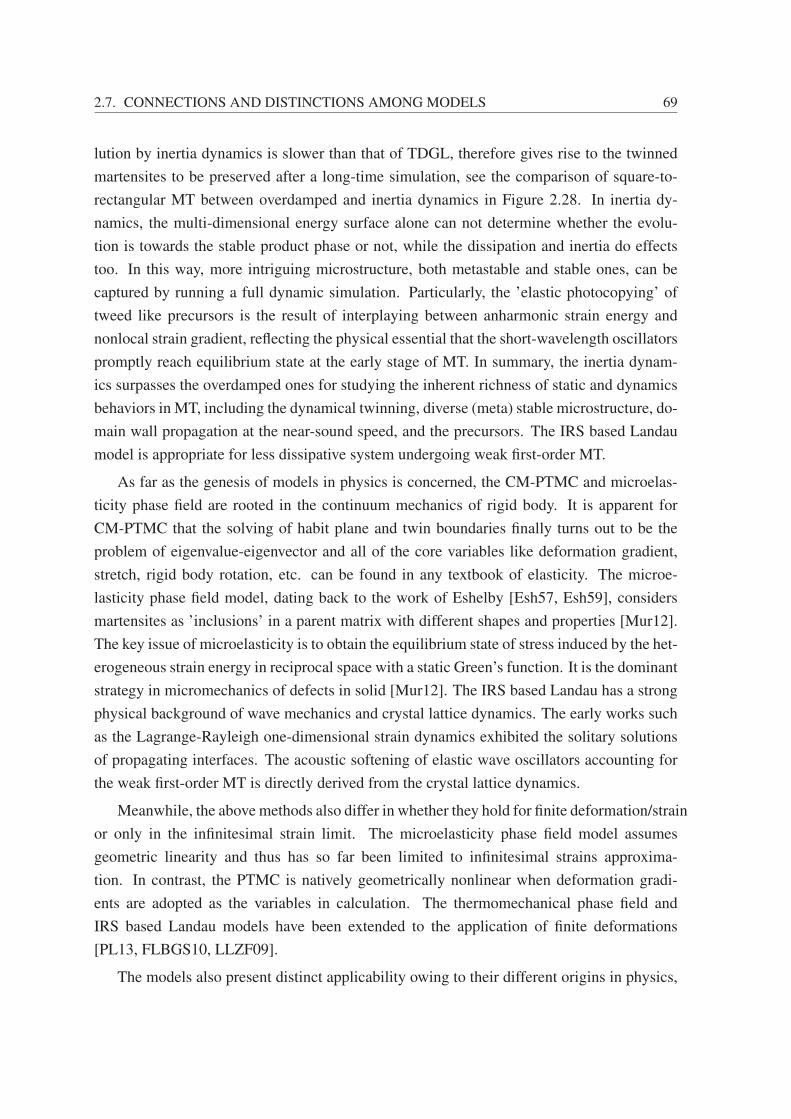
2.7. CONNECTIONS AND DISTINCTIONS AMONG MODELS 69
lution by inertia dynamics is slower than that of TDGL, therefore gives rise to the twinned
martensites to be preserved after a long-time simulation, see the comparison of square-to-
rectangular MT between overdamped and inertia dynamics in Figure 2.28. In inertia dy-
namics, the multi-dimensional energy surface alone can not determine whether the evolu-
tion is towards the stable product phase or not, while the dissipation and inertia do effects
too. In this way, more intriguing microstructure, both metastable and stable ones, can be
captured by running a full dynamic simulation. Particularly, the ’elastic photocopying’ of
tweed like precursors is the result of interplaying between anharmonic strain energy and
nonlocal strain gradient, reflecting the physical essential that the short-wavelength oscillators
promptly reach equilibrium state at the early stage of MT. In summary, the inertia dynam-
ics surpasses the overdamped ones for studying the inherent richness of static and dynamics
behaviors in MT, including the dynamical twinning, diverse (meta) stable microstructure, do-
main wall propagation at the near-sound speed, and the precursors. The IRS based Landau
model is appropriate for less dissipative system undergoing weak first-order MT.
As far as the genesis of models in physics is concerned, the CM-PTMC and microelas-
ticity phase field are rooted in the continuum mechanics of rigid body. It is apparent for
CM-PTMC that the solving of habit plane and twin boundaries finally turns out to be the
problem of eigenvalue-eigenvector and all of the core variables like deformation gradient,
stretch, rigid body rotation, etc. can be found in any textbook of elasticity. The microe-
lasticity phase field model, dating back to the work of Eshelby [Esh57, Esh59], considers
martensites as ’inclusions’ in a parent matrix with different shapes and properties [Mur12].
The key issue of microelasticity is to obtain the equilibrium state of stress induced by the het-
erogeneous strain energy in reciprocal space with a static Green’s function. It is the dominant
strategy in micromechanics of defects in solid [Mur12]. The IRS based Landau has a strong
physical background of wave mechanics and crystal lattice dynamics. The early works such
as the Lagrange-Rayleigh one-dimensional strain dynamics exhibited the solitary solutions
of propagating interfaces. The acoustic softening of elastic wave oscillators accounting for
the weak first-order MT is directly derived from the crystal lattice dynamics.
Meanwhile, the above methods also differ in whether they hold for finite deformation/strain
or only in the infinitesimal strain limit. The microelasticity phase field model assumes
geometric linearity and thus has so far been limited to infinitesimal strains approxima-
tion. In contrast, the PTMC is natively geometrically nonlinear when deformation gradi-
ents are adopted as the variables in calculation. The thermomechanical phase field and
IRS based Landau models have been extended to the application of finite deformations
[PL13, FLBGS10, LLZF09].
The models also present distinct applicability owing to their different origins in physics,

70 CHAPTER 2. MODELS OF MARTENSITIC TRANSFORMATION
Figure 2.28: The square-to-rectangular MT is simulated by overdamped (upper panel) and
inertia (bottom panel) dynamics with the same material and simulation parameters. The
numbers indicate the simulation time steps.
especially comparing microelasticity phase field model with IRS based Landau model. Based
on the previous discussion, we understand IRS based Landau model has advantages in rep-
resenting precursor, predicting transformation paths with anisotropic Onsager coefficients,
working with finite strains, monitoring displacement and deformation gradient and revealing
the underdamped nature. All these events are missing in microelasticity phase field model.
From Sections 2.3-2.5, we also found that the phase field models and IRS Landau model
are nearly equivalent in predicting the accurate twin plane and invariant plane consistent
with what PTMC predicts. However, phase field models possess an apparent advantage in
representing the habit planes. Few works for predicating habit plane between austenite and
internal twins have been reported by using IRS based Landau model, except for the theoret-
ical work of Barsch et al. [BHK87]. In contrast, it is a matured technique in all phase field
models, e.g. the Figure 2.23(b). It is because, the transformation strains are inputs of sim-
2.7. CONNECTIONS AND DISTINCTIONS AMONG MODELS 71
Figure 2.29: The simulated tweed structure in square-to-rectangular and triangle-to-
centered-rectangular [CKO+07] MTs.
ulation in phase field models, such that the so-called prediction is more like a morphology
recapturing with a set of scalar indicators of OPs η. However, in IRS based Landau, only
temperature dependent elastic coefficients are served as inputs. 1 Since the morphology is
represented by the OP strains shared by both austenite and martensites, the control of average
transformation strain with a ratio of two martensite variants becomes a challenge. Moreover,
neither of phase field and Landau models is capable of predicting the orientation relationship
deviated from the lattice correspondence because the extra freedom of rigid body rotation
without free energy change is not determined. The comparison of the applicability is listed
in Table 2.1.
Besides the aforementioned common ingredient and distinctions, one more point is wor-
thy being addressed between microelasticity phase field and IRS based Landau models. In
both methods, the homogeneous deformation with �k = 0 mode evolves at a constant rate, so
that the energy is not minimized with respect to the homogeneous part of the strain fields, ev-
idenced by the removal of the point �k = 0 in both Green’s functions in microelasticity phase
field and long-range integral kernel of OP strains. In fact, long-range integral kernel of OP
strains is formally a Green’s function. The only difference lies in the fact that the anharmonic
contribution of OP strains is not included in Green’s function of long-range integral kernel,
while harmonic heterogeneous relax energy contributed by all strain components is included
1If the high order elastic constants were available, the manipulating of Landau potential is avoided, such
that can lead to a true prediction.
72 CHAPTER 2. MODELS OF MARTENSITIC TRANSFORMATION
in Green’s function in microelasticity phase field.
In summary, while the models of MT stated in the thesis are endowed with the common
ingredient of energy minimization, they differ in the ways how to achieve the energy minima
and interface coherency. Different models have individual advantages and disadvantages in
predicting different properties.
2.8 Objectives
As is summarized in Section 2.7, the most complete model for MTs from the viewpoint of
the underlying physics is the Landau theory based on the IRS and inertia dynamics. However,
this approach has disadvantages from the application perspective. This doctoral thesis is
aimed at improving the IRS based Landau model towards advanced applications in structural
materials.
The specific objectives of the thesis are:
1. To develop a Landau model based on the irreducible representation of the point group
and transformation strains for MTs in polycrystals that describes accurately the microstruc-
tural features of polycrystalline ferroelastic materials.
2. Investigate the variant selection of martensites in polycrystals subjected to external
loading, and the dynamical nucleation of martensites in polycrystals under the combined
effect of external loading and temperature changes.
3. Develop a coupled model for displacive-diffusive transformations by integrating the
Landau model with information provided by thermo-kinetic calculation and database.
4. Extend the previous model to incorporate the effect of dislocations by incorporating
the continuum theory of dislocations.
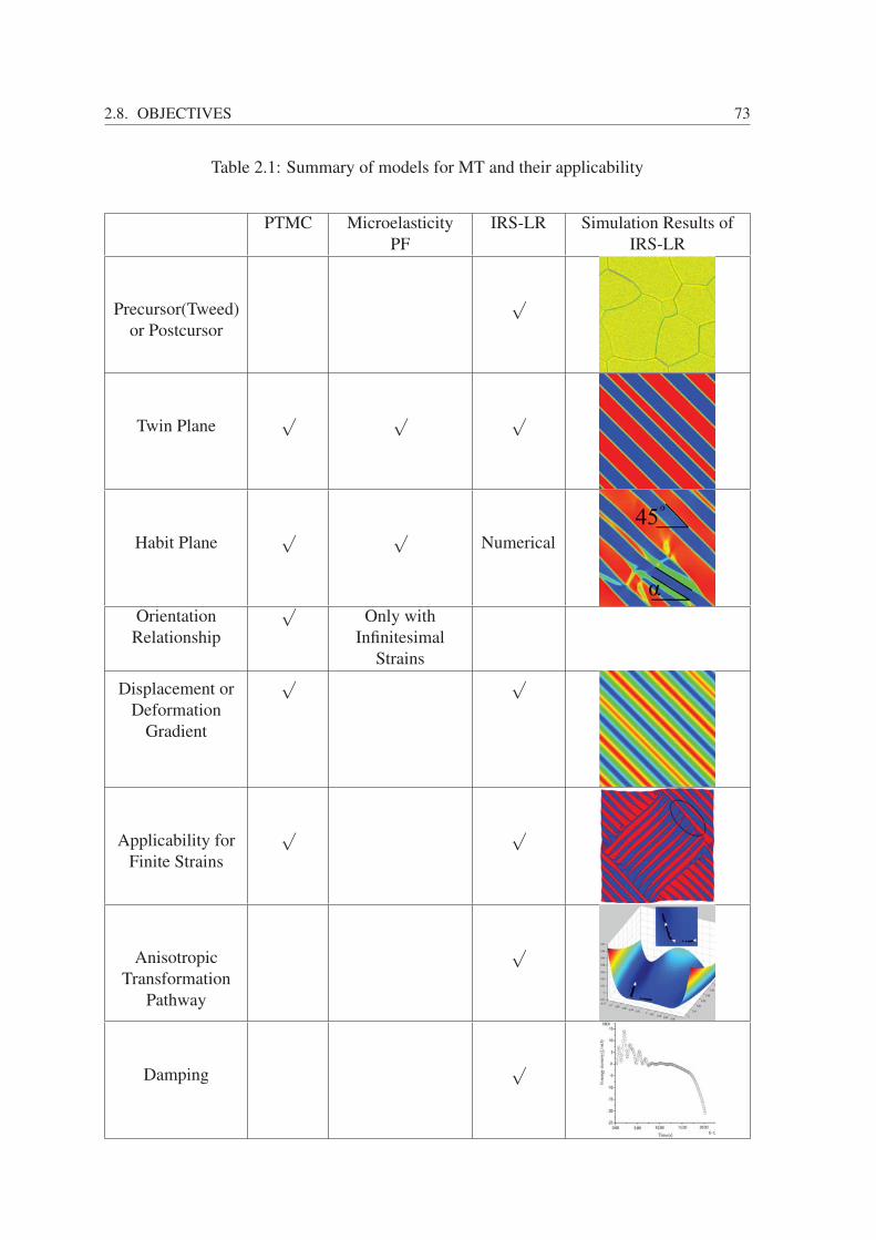
2.8. OBJECTIVES 73
Table 2.1: Summary of models for MT and their applicability
PTMC Microelasticity
PF
IRS-LR Simulation Results of
IRS-LR
Precursor(Tweed)
or Postcursor
√
Twin Plane√ √ √
Habit Plane√ √
Numerical
Orientation
Relationship
√Only with
Infinitesimal
Strains
Displacement or
Deformation
Gradient
√ √
Applicability for
Finite Strains
√ √
Anisotropic
Transformation
Pathway
√
Damping√

74 CHAPTER 2. MODELS OF MARTENSITIC TRANSFORMATION

Chapter 3Nonlinear Ginzburg-Landau Model ofMartensitic Transformation inPolycrystals
This work contains many things which are new and interesting. Unfortunately, everythingthat is new is not interesting, and everything which is interesting, is not new.
-Lev Landau
3.1 Introduction
We understand that crystalline materials of technological interest are always polycrys-
talline and include a very large number of grains with different grain orientations. Since
MTs occurring in polycrystals show some interesting features different from those in single
crystal, important progress has also been made on the modeling of MT in polycrystals with
the approaches revisited in chapter 2. Correspondingly, Bhattacharya [BS05] introduced the
fix-point iterative algorithm to evaluate the recoverable strains in polycrystalline SMAs un-
dergoing MTs in the language of continuum mechanics. Great success of modern phase-field
methods was achieved on this topic [AJK02, JAK01, HC14, MABÅ13a]. Recently, Heo et
al. [HC14] updated the micro-elasticity phase field model with a misfit strain relaxation
that permits elucidating the effects of elastic anisotropy and grain boundary curvature on
polycrystalline MTs. Malik et al. [MABÅ13a] used an elasto-plastic phase field model to
simulate the microstructure features of MTs in Fe-C alloy subjected to external loadings.
In the scheme of IRS, Ahluwalia et al. [ALS03, ALSA04] coupled grain orientations to
elastic strains in the over-damped TDGL dynamics to model the polycrystalline square-to-
rectangular MT and its response under the uniaxial tension, which was further extended by

76
CHAPTER 3. NONLINEAR GINZBURG-LANDAU MODEL OF MARTENSITIC
TRANSFORMATION IN POLYCRYSTALS
Cui et al. [CKO+07] to triangle-to-centered-rectangular case analogues to more complex
hexagonal-to-orthorhombic MT.
The IRS energetic scheme has proven useful to describe MT, and manifests itself by cap-
turing the nature of the damped system and propagated interfaces in proper MT once it was
applied with the Lagrange-Rayleigh dynamics [BG91, RG94, SLSB99]. Note that most of
the modeling for polycrystalline MTs adopted the TDGL dynamics in the past decades. Very
recently, utilizing Lagrange-Rayleigh dynamics with IRS based Landau energy (IRS-LR),
Ahluwalia et al. [AQW15] developed the 2-4-6 Landau polynomial with local symmetry-
adapted strains as OPs and then reformulated them in terms of global strains. They solved
the general equation of motion to investigate the grain size effects on the MT in nano-
polycrystalline Fe-Pd alloy and the stress-strain response in strain induced MT. Neverthe-
less, we believe their model is solely applicable to some nano-scale materials wherein the
martensitic nucleation and growth at grain boundaries were inhibited, or the effects of grain
orientations on martensite alignments 1 were smeared out by the dense grain boundary net-
work. However, the microscopic images of martensites generally show that the alignments of
martensite variants favor rotating certain angles with respect to the grain orientations in poly-
crystals, which is yet evidently recognized in the simulated microstructure of Ref.[AQW15].
In this chapter, we will modify the existing IRS-LR model to investigate the formation of
spatially varying martensite variants in polycrystals to include the following features: (1) the
transformation strains and characteristic microstructure signatures inside individual grains,
(2) the variation of the habit plane/twinning elements (i.e. twin/habit plane normal and shear
vector) of martensite, with different grain orientations, and (3) the microstructural change
due to external loading. By analyzing the simulated microstructure, we will gain insight into
how the IRS-LR model is connected with the CM-PTMC and, as a result, will demonstrate
physical inherency between these models and the theory.
3.2 Model
The physical nature of polycrystalline MTs, which shows the competition and constraints
between the martensite variants that are developed in each grain and the surrounding grains,
permits the grain orientation-transformation strain coupled field that need to be expressed
in a fixed global coordinate system. In single crystal model, Landau free energy is devel-
oped based on the linearized strain tensor with the component εij = 12(ui,j + uj,i), where
ui denotes the local displacement, and ui,j = ∂ui/∂xj is the displacement gradient in the
1in order to avoid any confusion, we use the alignment to describe the variants and twining and reserve the
orientation exclusively for grain orientation in square-to-rectangular case.
3.2. MODEL 77
intragranular coordinates. The symmetry-adapted linear strains εk, written in the linear com-
bination of the strain components, are selected as the OPs. Now we consider a MT in poly-
crystals: The real freedoms in a system undergoing MT are the global displacements, Ui, and
they should be connected with the OP strains by introducing an additional variable θ(r, t) de-
scribing grain orientation field. As such, the local strains and symmetry-adapted OP strains
are the functional of the global displacement gradients, viz. εij (UI,J) and εk (UI,J). In order
to distinguish the variables described in different references or coordinates, the variables in
global coordinates are denoted by capital letters while those in local coordinates by low-
ercase. The specific expressions of free energy and dynamic equations for the simulations
of 2D square-to-rectangular and triangle-to-centered-rectangular martensitic nucleation are
detailed as follows. As usual, the Landau free energy in the expansion of coupled OPs and
deterministic dynamic equations are still two key issues in Landau modeling.
3.2.1 Lagrange Description of Polycrystals
The starting point to work out a corrected IRS-LR model for polycrystals, as in Ref
[AQW15] and the phase field model [CY94], is to describe the grain orientation field of
polycrystals by defining the spatially distributed grain orientation θ (�η, r) with respect to
a set of arbitrarily selected intragranular coordinates which should serve as the reference
global system. Similar to Refs. [AQW15, CY94], θ is written as the functional of vectorial
indicator �η (η1, η2...ηQ),
θ (�η, r) =θm
Q− 1
[Q∑i=1
iηi
/Q∑i=1
ηi − 1
](3.1)
where the grain orientation i corresponds to ηi > 0 while the remaining components are
equal to zero. To obtain a coupled field, the grain orientation at the position r subsequently
enters the co-rotated local strain field expressed in global coordinates via a similarity trans-
formation with an orthogonal rotation matrix, i.e. E = R [θ (�η, t)] εRT [θ (�η, t)], where Eand ε are the strains in global and local coordinates, respectively, and R is rigid body rota-
tion matrix
[cos θ sin θ− sin θ cos θ
].
Unlike a TDGL dynamics with the IRS based Landau free energy functional, we explic-
itly express the Lagrangian incorporating the kinetic energy density T = ρU2/2 and the
Landau free energy density f as L=∫Vdr {T − f}, where ρ is the mass density, and U and
U stand for the displacement and the velocity in the global reference, thereby ensuring the
total energy density to be given in global coordinates. The free energy density f is intuitively
78
CHAPTER 3. NONLINEAR GINZBURG-LANDAU MODEL OF MARTENSITIC
TRANSFORMATION IN POLYCRYSTALS
defined as the summation of elastic energy density,felastic, the free energy density due to the
grain orientation
fgrain =
Q∑i=1
[ga12η2i +
ga22η3i +
ga32η4i
]+ga42
Q∑i=1
Q∑j>i
η2i η2j +
Q∑i=1
κg
2(∇ηi)
2(3.2)
and the free energy contribution due to the applied load fload, according to f := felastic +
fgrain+ fload, [CKO+07]. The elastic energy density felastic can be further divided into three
parts, i.e. local free energy density flocal, the energetic contribution originating from non-
OP strains fnon−OPs, and the gradient of OP strains fgrad. The first term flocal describes
the symmetry breaking during the phase transformation by adopting the symmetry-adapted
strains εi(r) as the independent OPs, i.e. linear combinations of the components of strain
tensor in intragranular coordinates. In case of the square-to-rectangular transformation, the
deviatoric strain ε2 = c2 (εxx − εyy) /2 is selected as the primary OP, so the local free energy
density is written as
flocal =A20
2
(T − Tc
Ms − Tc
)ε22 +
A4
4ε42 +
A6
6ε62 (3.3)
where A2 = A20
(T − Tc
Ms − Tc
)is temperature dependent deviatoric modulus, A4 and A6 are
related to higher order nonlinear elastic constants, and Tc and Ms are the critical point and the
MT starting temperature. While in the triangle-to-centered-rectangular case, both deviatoric
strain ε2 and shear strain ε3 = c3 (εxy + εyx) /2 are adopted as OPs, and the local free energy
density is formulated as
flocal =A20
2(T − Tc)
(ε22 + ε23
)+
B3
3
(ε32 − 3ε2ε
23
)+
A4
4
(ε22 + ε23
)2(3.4)
where B3 is the linear combination of third order elastic constants, and ci are symmetry-
related constants corresponding to individual MTs with c2 =√2, c3 = 1 for square-to-
rectangular and c2 = c3 = 1 for triangle-to-centered-rectangular in this work [PL13]. It is
noteworthy to point out that, Ahluwalia et al. [ALS03, ALSA04] and Cui et al. [CKO+07]
constructed the anharmonic Landau polynomials directly in global reference with TDGL dy-
namics and employed the St.-Venant’s compatibility condition in local reference. In contrast,
Ahluwalia et al.[AQW15] recently preserved the link between the local symmetry-adapted
OPs εi(r) and local strains εij in the intragranular coordinates [SSF12], and then rewrite
the local OP strains, the non-OP strains (e.g. local dilatation strain ε1 = c1 (εxx + εyy) /2)
and nonlocal gradient terms (e.g.(∇ε2)2
for square-to-rectangular) as the components of the
global displacement fields U, therefore express them in the reference coordinates for the
3.2. MODEL 79
Lagrangian. For example, the symmetry adapted deviatoric strain is expressed in global
displacements as,
ε2 = [ux,x (U, θ)− uy,y (U, θ)]/√
2
= [cos 2θ (UX,X − UY,Y ) + sin 2θ (UX,Y + UY,X)]/√
2(3.5)
where, U and u are displacements in different coordinates, and θ is the angle of grain orien-
tation in Eq.(3.1). The dilatation strain and shear strain are
ε1 = (εxx + εyy)/√
2 = (UX,X + UY,Y )/√
2
ε3 = (εxy + εyx)/2 = −sin(2θ)
2(UX,X − UY,Y ) +
cos(2θ)
2(UX,Y + UY,X)
(3.6)
This approach is followed in this chapter. The construction of Landau polynomials in global
and local reference would be equivalent only if the C11 − C12 = 2C44 (i.e. A2 = A3/2) is
rigidly satisfied in isotropic case and the contribution of the anharmonic terms is negligible
so that local free energy density degenerates in the full quadratic form.
3.2.2 Dynamical Equations
The evolution of grain orientation and displacement fields are treated differently in this
chapter. The TDGL equation
∂�η (r, t)
∂t= −Lη
δfgrainδ�η (r, t)
(3.7)
is used to describe the evolution of the OP field �η (r, t) of the grain orientations with Lη as
kinetic coefficient for interface mobility.
When the spatiotemporal evolution of displacements and strain fields is considered, a
variation method of Lagrange mechanics is utilized. By taking the variation of the La-
grangian with respect to the displacement U and U in the global reference and explicitly
substituting the Lagrangian into the Lagrange-Rayleigh equationsd
dt
δL
δUi
− δL
δUi
= −δR
δUi
,
the Lagrange-Rayleigh equations yield the general equations of motion in polycrystals
ρUi =∂
∂Xj
{∂f
∂εk
∂εk∂εpq
∂εpq∂Ui,j
−∇ · ∂f
∂∇εk
∂∇εk∂εpq
∂εpq∂Ui,j
+∂R
∂εk
∂εk∂εpq
∂εpq
∂Ui,j
}(3.8)
where, ρ is density, R and R are Rayleigh dissipation and dissipation density, written as
the functional of velocity of elastic waves to describe the friction in system. Generally, the
dissipative stress tensor should anisotropically depend on the space derivatives of the velocity
80
CHAPTER 3. NONLINEAR GINZBURG-LANDAU MODEL OF MARTENSITIC
TRANSFORMATION IN POLYCRYSTALS
field. For the sake of simplicity, an isotropic approximation of dissipation with viscosity is
utilized in this work. If the local stress expressed in global coordinates is defined as
σij =δF
δUi,j
=∂f
∂εk
∂εk∂εpq
∂εpq∂Ui,j
−∇ · ∂f
∂∇εk
∂∇εk∂εpq
∂εpq∂Ui,j
(3.9)
the dynamics of displacement fields is given by dissipative force balance equations
ρUi =∂σij
∂Xj
+ γ∇2Ui (3.10)
Different from Ref. [ALS03], the local stresses in our model enter dissipative force bal-
anced equations via the chain rule of functional differentiation of free energy with respect
to global displacement gradients. By numerical solving Eqs. (3.7) (3.9) and (3.10), the spa-
tiotemporal evolution of displacements, strains and grain orientations is obtained. Finally,
the viscous term drives the system to the mechanical equilibrium state. Moreover, in Al-
huwalia’s latest work with IRS-LR [AQW15], they took the global stress in the dissipative
force equation, leading to the global stress equilibrium in the laboratory reference. As such,
the morphology of martensite variants failed to exhibit the rotation of alignments across the
grain boundary. According to Mura [Mur12], the precondition of describing MT by the
displacement field is to assume that the elastic stress reaches its equilibrium instantly, as a
consequence the transformation strain components are derivatives of the total displacements.
In the case of polycrystals, the MT in individual grains should be equivalent when external
field is free. Thus, the stress in dissipative force equation should be the local transforma-
tion stress, i.e. the functional of the Landau free energy with respect to local transformation
strains expressed, however, in global reference.
Lookman et al. [LSR+03] derived the OP strain-based Bales-Gooding under-damped
dynamics by reformulating both non-OP strain(s) and strain compatibility in terms of OPs.
While the description with long-range OP strains has intrinsic advantages, e.g. the ability to
explicitly display the symmetry-specific compatibility kernels in both Fourier and real spaces
and to reveal the information of the energetically favored orientations and habit planes, the
same under-damped dynamics could be equivalently obtained via either the strain-based
Bales-Gooding or displacement-based Lagrange-Rayleigh descriptions. With the emphasis
to unveil the competency of displacement-based IRS-LR dynamics on describing orienta-
tions and habit planes and its connection with CM-PTMC, the displacement and displace-
ment gradients in this chapter are required to serve as inputs to kinematic compatibility equa-
tion of CM-PTMC for numerically solving the unit shear and habit/twin plane normal. To
this end, we choose the displacements U as the basic independent variables. By doing this,
the constraint of strain compatibility does not have to be solved explicitly [SLS10, RLS+01],
3.2. MODEL 81
and this is particularly useful when this model is extended to 3D.
3.2.3 Connection to CM-PTMC
In the IRS-LR model, the displacements are served as the basic independent variables.
They enter the OPs and Landau free energy via Eq.(2.66) in case of the infinitesimal strain
approximation. The information of the symmetry breaking has been included in the anhar-
monic terms in Landau free energy. Due to the transformation strains are small in most of
SMAs, the equi-energetic minima constructed by anharmonic Landau free energy to present
the martensite variants are located in the vicinity of original point of phase space. In the
regions far beyond the original point or when the anharmonic terms are fully ignored, the
Landau free energy shows a quadratic form, same as the one expressed in the linear elastic-
ity, i.e. f = σ : ε. In our polycrystalline model, the corotational or similarity transformation
of the strain tensor, E = RεRT, will not change the eigenvalues of right Cauchy-Green de-
formation tensor C =FTF, nor those of deformation gradient F. However, the common
eigenvectors of C and F in individual grains will be rotated with respect to the grain orien-
tations. Based on the established Landau free energy and dynamic equations, the martensite
morphology is achievable through eliminating the elastic stress inside the martensite do-
mains while the dissipative stress drives the system to a mechanical equilibriums state corre-
sponding to the minima of the potential energy. The dynamic processes are associated with
the formation, growth and propagation of the interface between phases/domains by solving
Eq.(3.8) or (3.10). Reviewing Eq. (3.10), this equation is actually a general form of the
momentum balance ρU = ∇ ·Σ in continuum mechanics, if no Rayleigh dissipation is con-
sidered, where Σ is the corotational stress tensor given by Σ = RσRT, which essentially
reflects a direct coupling of primary OP to grain orientation in Eq.(3.9)
With this dynamic equation, when the mechanical equilibrium state coincides with the
phase equilibrium between martensite and austenite, the evolution of the system means also
its seeking the lattice correspondence, e.g. the Bain correspondence in cubic-to-tetragonal
MT. In essence, most of the key elements, including the displacement related transforma-
tion strains, the lost symmetry elements when undergoing MT to form twin planes, and
the lattice correspondence obtained from energy minimization, are common to CM-PTMC
and IRS-LR theories. As a consequence, the final state of martensitic morphology and mi-
crostructure features, like twin/habit plane, twinning shear, invariant plane shear, etc. con-
veyed by expressions in CM-PTMC, can be equivalently captured by IRS-LR modeling.
However, some intrinsic distinctions, both in statics and dynamics, between the two theories
can be addressed. In general, the CM-PTMC and IRS-LR are analogous to rigid-body and

82
CHAPTER 3. NONLINEAR GINZBURG-LANDAU MODEL OF MARTENSITIC
TRANSFORMATION IN POLYCRYSTALS
wave mechanics for describing the same MT. The distinctness resulting from the dynamics,
as Lookman et al. elaborated in Ref. [LSR+03], is related to the under-damped nature of
IRS-LR. As for the statics, it lies in the higher gradient regularization along with the anhar-
monic contribution included in the IRS based free energy. In addition, since the IRS based
Landau potential does not explicitly use the lattice parameters as inputs, the deviation of the
real habit plane from the ideal lattice correspondence plane can only be numerically handled
by the coupling between OP and non-OP strains. The analytic solution of the dependence of
habit plane on lattice parameters between austenite and internal twins for IRS-LR or stain-
only Bale-Gooding dynamics is still on working. In the following sections, we implement
the numerical simulation to reveal and verify our IRS-LR model of MT in polycrystals, as
exemplified in 2D square-to-rectangular and triangle-to-centered-rectangular cases, and to
understand the simulated microstructure by itemizing and referring to the common ingredi-
ents of the analytical CM-PTMC.
3.3 Numerical Implementation
Upon the proposed model, we started our simulation with generating a polycrystalline
microstructure of austenite. Our simulations were carried out using a Fast Fourier Trans-
formation (FFT) based spectral method under periodic boundary conditions in 256 × 256
grids with 5 grain orientations of 0◦, 7.5◦, 15◦, 22.5◦ and 30◦ (= θmax), respectively (Fig
3.1a). For the formation of the polycrystalline structure, we used the parameters, ga1 =
−1, ga2 = −1, ga3 = 1, and ga4 = 2. kg was adjustable to produce appropriate configura-
tion. While the model is developed for generic materials undergoing square-to-rectangular
and triangle-to-centered-rectangular transformations, we chose the Fe-Pd alloy in these sim-
ulations as the representative of square-to-rectangular in 2D as the analog of 3D cubic-to-
tetragonal MT and the Mg-Cd alloy for triangle-to-centered-rectangular as the analog of
hexagonal-to-orthorhombic, respectively. For Fe-Pd ferroelastic alloy, the following mate-
rials parameters were chosen based on the experimental results of elastic constants:A1 =
333.91GPa,A20 = 11.5GPa,A3 = 282GPa,A4 = −1.7 ∗ 103GPa, Tm = 295K and
Tc = 270K [GLS08, MOF90, ALS03]. It is noted that the temperature dependence of the
elastic constant A2 in experiments and linear fitting was well represented by the parameter
A2 = A20T − Tc
Ms − Tc
in simulations, while the other elastic constants were unchanged with
temperature for simplicity. A6 was determined from A20, A4, and quenching temperature T ,
satisfying the constraints of Landau polynomial for first-order transformation in Ref. [Fal80].
The value of gradient coefficient was set to g = 3.0 ∗ 10−8 [AQW15, ALSA04] based on

3.4. MICROSTRUCTURE ANALYSIS 83
microstructure observation, while the dissipation coefficient was estimated as 0.015Ns/m2
according to Ref. [ALSA04]. Upon these parameters, the interface energy density of full
twinned martensites can be estimated around 0.5J/m2 from multi-well degenerated Landau
free energy near the critical point2. The retrieved value of interface energy density in our
simulation has the correct order of magnitude, consistent with theoretical estimations and
first principles calculations [OC76, WCLM10]. While the corresponding MgCd parameters
were A1 = 45.8GPa,A20 = 10.9GPa,B3 = −1.35∗103GPa,A4 = 2.0A23/ (9.0 |A2|), and
Tc = 526K [GSZ+09, VC12]. To tackle the numerical instability, the materials and simula-
tion parameters were subjected to a normalization by following [Sal09], wherein the spatial
and energetic variables were rescaled by introducing normalization factors d0 = 7 ∗ 10−9m
and f0 ∼ 1010J , respectively; such that x = x/d0, and Ai = Ai/f0. The time scale was
rescaled as t = t/t0 = t/√
ρd20/f0, and the rescaled viscosity is γ = γ/(
d0√f0ρ). At
the beginning of simulation, the random fluctuations of displacements ζuiobtained from a
Gaussian noise were introduced. The mean and correlation of fluctuations satisfy
〈ζui(r, t)〉 = 0,
⟨ζui
(r, t) ζuj(r′, t′)
⟩= 2γkBTρδ (r− r′) δ (t− t′) (3.11)
More details of the model and of the numerical implementation can be found in Refs.
[CKO+07, Sal09].
3.4 Microstructure Analysis
3.4.1 Polycrystalline Microstructure of Square -to- Rect-angular Martensites
A 2D polycrystalline structure of the parent austenite with randomly distributed grains is
shown in Figure 3.1a. The grains with different orientations are displayed in different colors,
along with the values of the grain mis-orientation angles with respect to the reference blue
grain. Figure 3.1b illustrates the snapshot of the morphology of the square-to-rectangular
polycrystals without external loading encoded by a combination of the deviatoric strain ε2
and the grain orientation angle. In the grains with orientation θ = 0, the domain morphology
is characterized by two different types of martensite variants, i.e. red and blue ones, with
opposite stretch tensors alternatively arranged. The twin boundaries are stretching in the
directions of ±π/4. Further inspection of the microstructure in each grain of the polycrystal
2If the viscous term is removed, the conservation equation of motion utilized in our simulation describes
a physical picture that the dropping local free energy in Landau potential triggers the formation of the habit
planes and/or twin boundaries during the martensitic nucleation and drives the interface propagation during
martensite growth. In fact, the existence of viscous term will minimize the finite kinetic energy density.

84
CHAPTER 3. NONLINEAR GINZBURG-LANDAU MODEL OF MARTENSITIC
TRANSFORMATION IN POLYCRYSTALS
reveals that they present the very same features of the single crystal but simply rotate to align
with their respective grain orientations, e.g. the perpendicular lath variants in the grains with
orientation θ = π/12 (green grains in Figure 3.1a) turn to align along the π/3 and 5π/6
orientations with respect to the horizontal X axis of the global reference. Some needle-
like martensites with tapering tips occur in the θ = π/6 grain, resulting from reducing
the interface energy when the variants with the orientation alignments of (±π4 + π/6) are
anticipated to intersect each other. If finite strain is considered, bending will occur at the
tips of variants [FLBGS10]. Note that the alignments of martensite variants in individual
grain rotate certain angle in accordance with the grain orientation in global reference as
evidenced in Ahluwalia’s work when using the Landau energetics with TDGL dynamics
[ALS03, ALSA04]. Unfortunately, it was unclearly shown in his latest work by using LR
dynamics [AQW15]. This has been significantly improved in our IRS-LR model.
3.4.2 Polycrystalline Microstructure of Triangle -to- Centered-Rectangular Martensites
The intricate microstructures in the triangle-to-centered-rectangular polycrystals, visual-
ized by shear strain ε3, are shown in Figure 3.1c, wherein three distinguishable centered-
rectangular martensite variants (i.e. red, blue and green) build various polygonal patterns in-
cluding rectangular, rhombus, trapezoidal, etc. More interestingly, the self-accommodation
of variants leads to the intriguing nested-stars pattern in triangle-to-centered-rectangular
transformation, while the collision of domain walls gives rise to the formation of various
types of junctions or nodes. As expected, the nested and un-nested stars (highlighted by
circles in Figure 3.1c), as well as the characteristic nodes, such as (1,3,5,3) (2,5,5), (1,4,7),
(1,1,10) and (1,3,5,3) (following the notation of Curnoe et al. [CJ01a]), are found in the
simulated triangle-to-centered-rectangular patterns. Moreover, a small number of imper-
fect (1,1,1,1,1,7) nodes and many spiral branched patterns containing (1,3,5,3) nodes are
observed since a relatively large bulk modulus associated with Mg-Cd alloys is used in
our simulation. All the patterns and/or nodes well represent the morphology in Mg-Cd
alloy undergoing the analogous hexagonal-to-orthorhombic MT characterized by Kitano
[KKK88, KK91] et al. and Sinclair et al. [SD77]. The high resolution TEM images with
the node notations are compared with our simulated pattern in Figure 3.2. Inside individual
grains, the optimal arrangement of CR variants with respect to their grain orientations can
be recognized by tracking the directions of domain walls that connect red and blue vari-
ants in the spiral branched pattern. The twin boundary stretches along the global X axis in
the grain θ = 0, and perfectly changes to 7.5◦, 15◦ and 30◦ in the grains with orientations
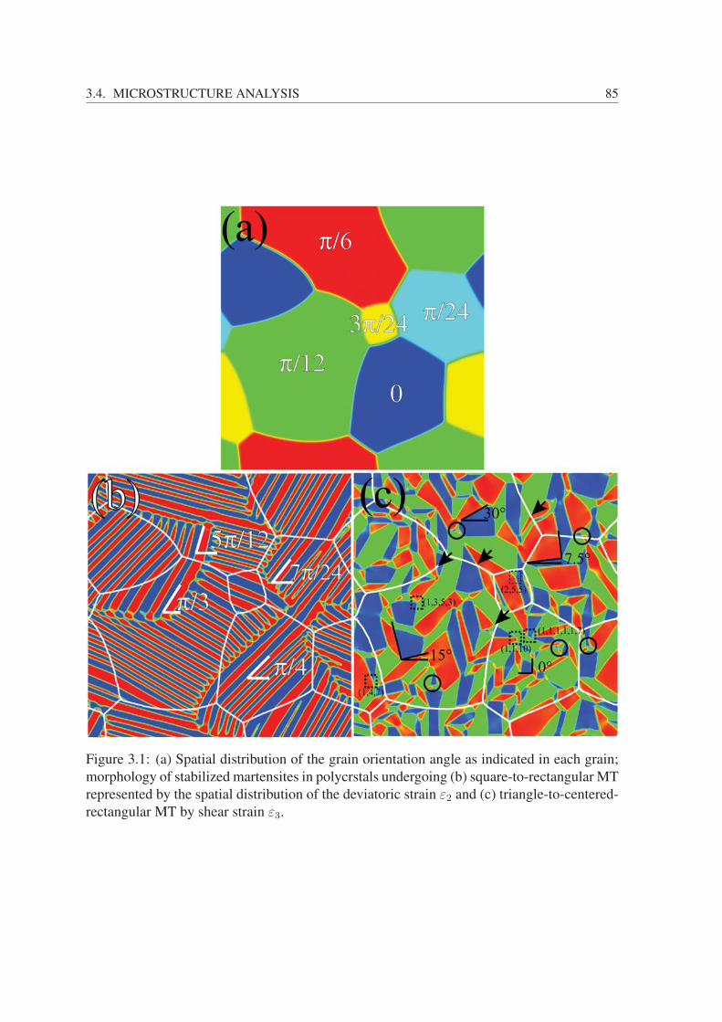
3.4. MICROSTRUCTURE ANALYSIS 85
Figure 3.1: (a) Spatial distribution of the grain orientation angle as indicated in each grain;
morphology of stabilized martensites in polycrstals undergoing (b) square-to-rectangular MT
represented by the spatial distribution of the deviatoric strain ε2 and (c) triangle-to-centered-
rectangular MT by shear strain ε3.
86
CHAPTER 3. NONLINEAR GINZBURG-LANDAU MODEL OF MARTENSITIC
TRANSFORMATION IN POLYCRYSTALS
θ = π/24, π/12 and π/6, respectively, following the angles indicated in Figure 3.1c. How-
ever, not all of the domain walls show the perfect rotations, i.e. the twin boundaries between
the same correspondence variant pair of martensites at different nodes exhibit some devia-
tions from the ideal angles. For example, the directional angles of the domain walls connect-
ing red and green variants in the (1,1,1,1,1,7) nodes are 30.3◦ and 120.9◦ (with the difference
between being close to π/2) in the bottom-right θ = 0 grain in comparison with 33.8◦ and
137.9◦ in the neighboring (2,5,5) nodes (see Figure. 3b and 3c). This reveals a deviation of
less than +1.0◦ from the ideal rigid body rotations of (π/6+nπ/2) in (1,1,1,1,1,7) nodes and
of positive +3.8◦ or negative -2.1◦ in (2,5,5) nodes. Meanwhile, the domain walls between
red and green variants in the θ = π/12 grain have directional angles of 45.0◦ in (1,3,5,3)
node and 42.8◦ in (2,5,5) node (Figure 3.3c) with respect to global X axis. Therefore, they
extend towards 30.0◦ and 27.8◦ for these two nodes in intragranular coordinates, and present
a vanishing deviation in (1,3,5,3) node but a negative deviation of -2.2◦ in (2,5,5) node.
Thus, we conclude that the triangle-to-centered-rectangular variants (also the domain walls)
rotate by an approximate angle from their respective grain orientations, while the deviation
from ideal angles is related to "disclination". The ideal domain walls in the spiral branched
pattern are ascribed to the assembly of the four disclination-free (1,3,5,3) nodes. The for-
mation of (1,1,1,1,1,7) node, as analyzed by Curnoe [CJ01a] and Kitano [KKK88, KK91],
accompanies with disclination angle of 0.24◦. In the case of the (2,5,5) node, it shows two
disclination angles of -2.92◦ and 2.72◦ depending on the mirror (m) or rotation (r) type of
the twin boundaries. The simulated results reveal the same trend of the variation of discli-
nation angles for different nodes. In a simulation conditioned with the infinitesimal strain
approximation, it is difficult to accurately measure a disclination angle because the angles of
disclination at a particular node will be smeared out and/or shared by the deviated domain
walls. And the larger disclination angle at a node, the larger deviation would display at the
simulated domain walls.
For the triangle-to-centered-rectangular, some transitive and irregular martensite variants
and domain walls persist even at the late growth stage in Figure 3.1c. This departure from full
relaxation configurations reflects the propagation and collision of elastic waves in polycrys-
tals. During the MT, the effective long-range interactions between the strains are generated,
so the creation or vanishing of a domain requires a global change in the displacement field
across different grains. The adjustment of the displacement or the deformation gradient field
is the consequence of competitive effects of the twinning orientations that originate from
transformation strains of MT and misorientations among grains, respectively. As already
discussed, the geometry compatibility is always obeyed in our model, and not all charac-
teristic twin boundaries can be perfectly satisfied to form the pairs (groups) of fascinating

3.5. DISCUSSION 87
Figure 3.2: The simulated characteristic domain configurations are in comparison with
observed (HR)TEM images with the notations of various boundary nodes during the 3D
hexagonal-to-orthorhombic MT in Mg-Cd system [SD77, KKK88, KK91].
patterns assembled by martensite variants, thus leading to a few isolated martensite vari-
ants. It is more clearly evidenced by the fact that the morphology of the triangle-to-centered-
rectangular martensite in the vicinity of grain boundaries exhibits complicate patterns, unlike
the sole "kink" in the square-to-rectangular case.
3.5 Discussion
3.5.1 Understand the Microstructural Features in the Per-spective of CM-PTMC
The symmetry permissible orientations of domain walls in square-to-rectangular and
triangle-to-centered-rectangular single crystal (or 3D cubic-to-tetragonal and hexagonal-to-
orthorhombic) martensites have been theoretically investigated by Aizu [Aiz69], Sapriel
[Sap75], Boulesteix et al. [BYS+86], Manolikas et al. [MA80a, MA80b], and Bender-
sky [BB93], following equivalent methodologies as the prototypical PTMC contributed by
Bowles et al. [BM54a, MB54, BM54b] and Wechsler et al. [Wec59, WRL60], and later inter-
preted by Wayman [Way64]. Hatch et al. [HLSS03] thoroughly elucidated the domain wall
orientations for all of the 2D ferroelastic martensites and calculated the directions of ideal
habit planes based on the long-range compatibility kernel in Fourier space and homogenous
quadratic equation in spatial space. In square-to-rectangular martensitic single crystal, the
orientations of domain walls are the reflection planes with the directions of multiples of π/4,

88
CHAPTER 3. NONLINEAR GINZBURG-LANDAU MODEL OF MARTENSITIC
TRANSFORMATION IN POLYCRYSTALS
which are symmetry elements of parent phase but no longer persist in martensite variants.
This can be verified by the fact that reflection planes with the plane normal n = [1, 1] or
[1,−1] satisfy Eq.(2.72) and as twin boundaries under the predefined transformation strains
α
[1 00 −1
]and α
[ −1 00 1
]corresponding to the strains of red and blue martensite vari-
ants in the θ = 0 grain (the dark blue grain in Figure 3.1a) at the final state of our simulation.
The simulated twin boundaries with the directions of ±π/4 in Figure 3.1b are consistent
with the analysis based on the group theory and CM-PTMC. It thus concludes that the elas-
tic strain is expelled from martensite domains in the numerical implementation of the IRS-
LR model, leaving transformation strains as the indicators for individual martensite variants
at the final state. Nevertheless, the kinematic compatibility in Eqs.(2.72) and (2.76) in the
polycrystals should be rewritten into Eq.(3.12) following the orthogonal transformation of
the transformation strain E = RεRT. It gives rises to the kinks/rotations of both twin plane
normal n and shear vector a by a specific angle with respect to their grain orientations when
the twin reaches a grain boundary. It explains why the martensite turn to align along the
(7π/24, 19π/24), (π/3, 5π/6), (3π/8, 7π/8) and (5π/12, 11π/12), respectively, in the grains
θ = π/24, π/12, π/8 and π/6 as shown in Figure 3.1b. Another peculiarity of polycrys-
talline patterns in our square-to-rectangular simulation is that certain variant seeks to retain
its variant type when passing a grain boundary. This is because the displacements, as the ba-
sic independent variables, impose the geometry compatibility as a prior condition. Following
the argument of Bhattacharya [Bha03], the variant with same sub-matrix of the strain tensor,
i.e. the same variant in our 2D case, is automatically selected when the front of the elastic
wave propagates across the grain boundary. If there is a spatial inhomogeneous distribution
of the residual localized stress accumulated at grain boundaries, the grain boundaries may
arrest the growth of individual martensite variant, yet induce the other martensite variant at
the other side of the grain boundary.
EI − EJ = R(εI − εJ
)RT =
1
2(Ra⊗Rn+Rn⊗Ra) ;
∇U = Rb⊗Rm(3.12)
Similarly, Eq.(3.12) in PTMC can also be visualized in our numerical benchmark of
the IRS-LR for polycrystalline triangle-to-centered-rectangular MT. In the single crystal
triangle-to-centered-rectangular MT, the orthogonal transformation with a rotation of 2π/3
for eI = ζ
[1 00 −1
]in the coordinates of orthogonal axis of CR phase generates two other
martensite variants with the transformation strains eII = ζ
[ −1/2 −√3/2
−√3/2 1/2
]and eIII =
ζ
[ −1/2√3/2√
3/2 1/2
]. Defining the variants II and III with Eq.(2.72), two orthogonal planes
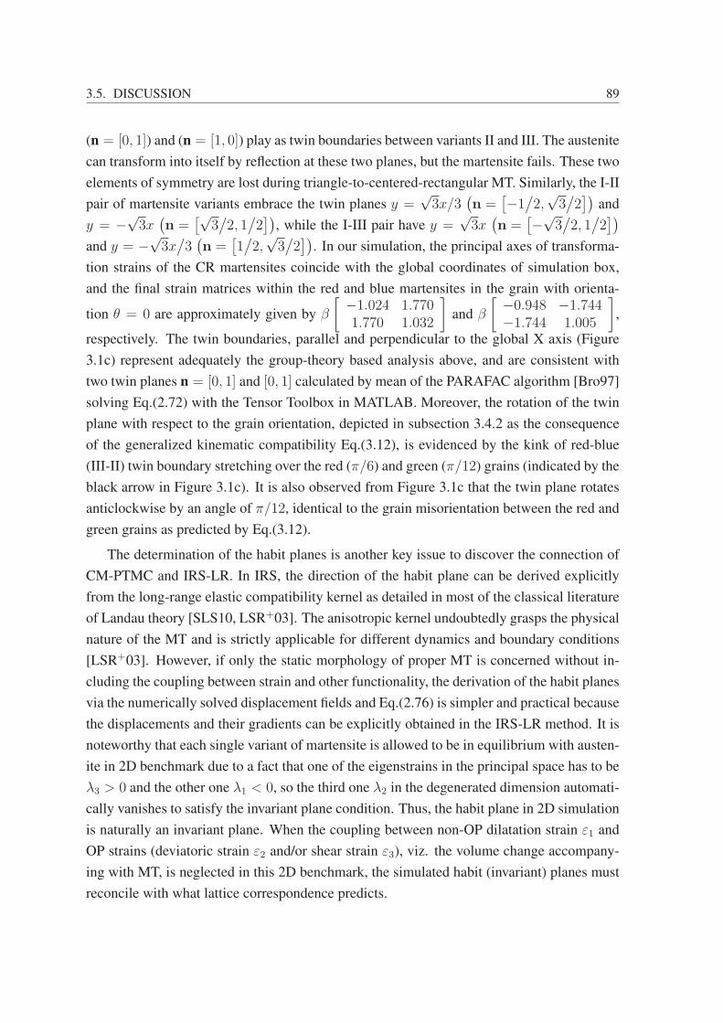
3.5. DISCUSSION 89
(n = [0, 1]) and (n = [1, 0]) play as twin boundaries between variants II and III. The austenite
can transform into itself by reflection at these two planes, but the martensite fails. These two
elements of symmetry are lost during triangle-to-centered-rectangular MT. Similarly, the I-II
pair of martensite variants embrace the twin planes y =√3x/3
(n =
[−1/2,√3/2])
and
y = −√3x(n =
[√3/2, 1/2])
, while the I-III pair have y =√3x(n =
[−√3/2, 1/2])
and y = −√3x/3(n =
[1/2,√3/2])
. In our simulation, the principal axes of transforma-
tion strains of the CR martensites coincide with the global coordinates of simulation box,
and the final strain matrices within the red and blue martensites in the grain with orienta-
tion θ = 0 are approximately given by β
[ −1.024 1.7701.770 1.032
]and β
[ −0.948 −1.744−1.744 1.005
],
respectively. The twin boundaries, parallel and perpendicular to the global X axis (Figure
3.1c) represent adequately the group-theory based analysis above, and are consistent with
two twin planes n = [0, 1] and [0, 1] calculated by mean of the PARAFAC algorithm [Bro97]
solving Eq.(2.72) with the Tensor Toolbox in MATLAB. Moreover, the rotation of the twin
plane with respect to the grain orientation, depicted in subsection 3.4.2 as the consequence
of the generalized kinematic compatibility Eq.(3.12), is evidenced by the kink of red-blue
(III-II) twin boundary stretching over the red (π/6) and green (π/12) grains (indicated by the
black arrow in Figure 3.1c). It is also observed from Figure 3.1c that the twin plane rotates
anticlockwise by an angle of π/12, identical to the grain misorientation between the red and
green grains as predicted by Eq.(3.12).
The determination of the habit planes is another key issue to discover the connection of
CM-PTMC and IRS-LR. In IRS, the direction of the habit plane can be derived explicitly
from the long-range elastic compatibility kernel as detailed in most of the classical literature
of Landau theory [SLS10, LSR+03]. The anisotropic kernel undoubtedly grasps the physical
nature of the MT and is strictly applicable for different dynamics and boundary conditions
[LSR+03]. However, if only the static morphology of proper MT is concerned without in-
cluding the coupling between strain and other functionality, the derivation of the habit planes
via the numerically solved displacement fields and Eq.(2.76) is simpler and practical because
the displacements and their gradients can be explicitly obtained in the IRS-LR method. It is
noteworthy that each single variant of martensite is allowed to be in equilibrium with austen-
ite in 2D benchmark due to a fact that one of the eigenstrains in the principal space has to be
λ3 > 0 and the other one λ1 < 0, so the third one λ2 in the degenerated dimension automati-
cally vanishes to satisfy the invariant plane condition. Thus, the habit plane in 2D simulation
is naturally an invariant plane. When the coupling between non-OP dilatation strain ε1 and
OP strains (deviatoric strain ε2 and/or shear strain ε3), viz. the volume change accompany-
ing with MT, is neglected in this 2D benchmark, the simulated habit (invariant) planes must
reconcile with what lattice correspondence predicts.

90
CHAPTER 3. NONLINEAR GINZBURG-LANDAU MODEL OF MARTENSITIC
TRANSFORMATION IN POLYCRYSTALS
Figure 3.3: (a) The calculated invariant plane normals in square-to-rectangular polycrys-
talline martenstie are represented by white arrows. The two perpendicular invariant plane
normals in grains with θ > 0 anticlockwise rotated the corresponding angles approximat-
ing the grain misorientation angles with respect to the alignment of ±π/4 in the grain with
θ = 0. (b)-(c) The magnifying morphology of characteristic domains exhibit the minor dis-
crepancies of the directional angles of the particular boundaries in various nodes, implying
the information of disclination. (b) and (d) illustrate the calculated invariant plane normals
in various domains of individual grains.

3.5. DISCUSSION 91
Therefore, the most possible invariant plane normals and lattice correspondence shears
could be estimated by decomposing numerically the displacement gradient tensor Ui,j into
the dyadic product of two vectors by the PARAFAC algorithm, although they are not unique
solutions. The arrows illustrated in Figure 3.3 are the calculated invariant plane normals
in the vicinity of the characteristic patterns. In Figure 3.3a, the invariant plane normals
of the square-to-rectangular case aligns with the same directions as the twin plane normal.
Although the vectors point in different directions in individual grains, they all imply the
[1, 1] or [1,−1] crystallographic indexes of austenite, consistent with the invariant plane nor-
mal predicted by PTMC with the Bain correspondence. Figure 3.3b displays the calculated
invariant normals of triangle-to-centered-rectangular martensites at the (1, 1, 1, 1, 1, 7) and
(2, 5, 5) nodes next to the spiral branched pattern in the grain with the orientation θ = 0. The
invariant normals of the green martensite point to ±π/4 in the global coordinates, which
are associated with [1, 1] and [1,−1] directions of tetragonal axes. These findings are in
good agreement with those predicted by Sapriel [Sap75] and Boulesteix [BYS+86] for sin-
gle crystal hexagonal-to-orthorhombic martensite with the PTMC [Way64]. Moreover, the
red and blue domains at the very (2, 5, 5) node exhibit the directions of invariant plane nor-
mals of 7π/12 and 5π/12. It is apparent that the invariant plane normal of the blue domain
is directly related to that of green domain (−π/4) via a symmetry operation of 3-folded rota-
tion, whereas red domain adopts the perpendicular solution for the invariant plane normal in
Eq.(2.76). As a consequence, not all of the invariant planes at a node are 3-folded rotational
related. Figure 3.3d illustrates the calculated invariant plane normals in the nested star. The
red, blue and green martensite variants of clover leaves with the same area are related by
3-folded rotation, but they have no common twin boundaries each other. Among them, the
outer green martensite shows the invariant plane normal at the direction of −π/6 referenc-
ing to the global X axis. Because the nested star is located in the grain with the orientation
angle of π/12, the direction angle is a sum of direction angles of invariant plane normal
in single crystal and the grain orientation (−π/4 + π/12 = −π/6), meaning that invariant
plane normal would rotate by the angles of the grain orientation as what Eq.(3.12b) requires.
From the comparison between the results of IRS-LR simulation and CM-PTMC analysis de-
tailed above, it concludes that most of the simulated microstructural features by IRS-LR are
in good agreement with what kinematic compatibility equation predicts in CM-PTMC. It is
due to the common ingredients, including lattice correspondence, kinematic compatibility,
crystal symmetry etc., that the results of IRS-LR model in equilibrium state is proven to rest
consistency with CM-PTMC.
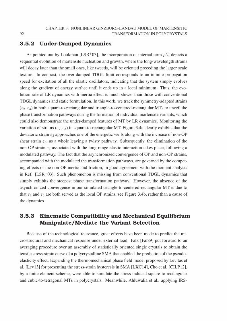
92
CHAPTER 3. NONLINEAR GINZBURG-LANDAU MODEL OF MARTENSITIC
TRANSFORMATION IN POLYCRYSTALS
3.5.2 Under-Damped Dynamics
As pointed out by Lookman [LSR+03], the incorporation of internal term ρUi depicts a
sequential evolution of martensite nucleation and growth, where the long-wavelength strains
will decay later than the small ones, like tweeds, will be oriented preceding the larger scale
texture. In contrast, the over-damped TDGL limit corresponds to an infinite propagation
speed for excitation of all the elastic oscillators, indicating that the system simply evolves
along the gradient of energy surface until it ends up in a local minimum. Thus, the evo-
lution rate of LR dynamics with inertia effect is much slower than those with conventional
TDGL dynamics and static formulation. In this work, we track the symmetry-adapted strains
(ε2, ε3) in both square-to-rectangular and triangle-to-centered-rectangular MTs to unveil the
phase transformation pathways during the formation of individual martensite variants, which
could also demonstrate the under-damped features of MT by LR dynamics. Monitoring the
variation of strains (ε2, ε3) in square-to-rectangular MT, Figure 3.4a clearly exhibits that the
deviatoric strain ε2 approaches one of the energetic wells along with the increase of non-OP
shear strain ε3, as a whole leaving a twisty pathway. Subsequently, the elimination of the
non-OP strain ε3 associated with the long-range elastic interaction takes place, following a
modulated pathway. The fact that the asynchronized convergence of OP and non-OP strains,
accompanied with the modulated the transformation pathways, are governed by the compet-
ing effects of the non-OP inertia and friction, in good agreement with the moment analysis
in Ref. [LSR+03]. Such phenomenon is missing from conventional TDGL dynamics that
simply exhibits the steepest phase transformation pathway. However, the absence of the
asynchronized convergence in our simulated triangle-to-centered-rectangular MT is due to
that ε2 and ε3 are both served as the local OP strains, see Figure 3.4b, rather than a cause of
the dynamics
3.5.3 Kinematic Compatibility and Mechanical EquilibriumManipulate/Mediate the Variant Selection
Because of the technological relevance, great efforts have been made to predict the mi-
crostructural and mechanical response under external load. Falk [Fal89] put forward to an
averaging procedure over an assembly of statistically oriented single crystals to obtain the
tensile stress-strain curve of a polycrystalline SMA that enabled the prediction of the pseudo-
elasticity effect. Expanding the thermomechanical phase field model proposed by Levitas et
al. [Lev13] for presenting the stress-strain hysteresis in SMA [LXC14], Cho et al. [CILP12],
by a finite element scheme, were able to simulate the stress induced square-to-rectangular
and cubic-to-tetragonal MTs in polycrystals. Meanwhile, Ahluwalia et al., applying IRS-
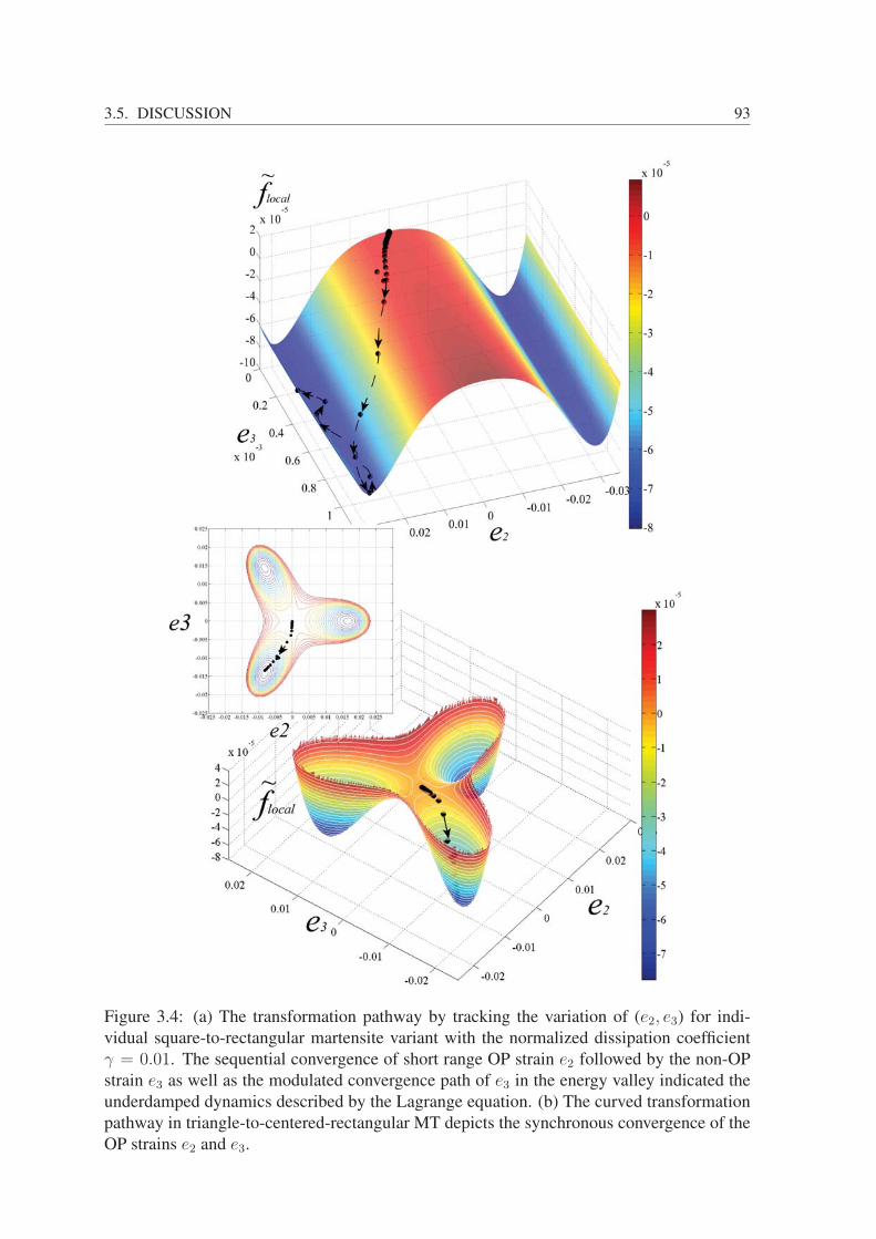
3.5. DISCUSSION 93
Figure 3.4: (a) The transformation pathway by tracking the variation of (e2, e3) for indi-
vidual square-to-rectangular martensite variant with the normalized dissipation coefficient
γ = 0.01. The sequential convergence of short range OP strain e2 followed by the non-OP
strain e3 as well as the modulated convergence path of e3 in the energy valley indicated the
underdamped dynamics described by the Lagrange equation. (b) The curved transformation
pathway in triangle-to-centered-rectangular MT depicts the synchronous convergence of the
OP strains e2 and e3.
94
CHAPTER 3. NONLINEAR GINZBURG-LANDAU MODEL OF MARTENSITIC
TRANSFORMATION IN POLYCRYSTALS
TDGL [ALS03, ALSA04] and IRS-LR [AQW15] models respectively, simulated the poly-
crystalline square-to-rectangular MT under uniaxial tensile loading and predicted the stress-
strain response as a function of strain rate.
In this chapter, we utilize the modified IRS-LR approach to explore the morphological
change of the martensite variants in polycrystals under uniaxial external loading. Choosing
the global X axis as the uniaxial loading direction, its contribution to the energy density is
expressed as fload = −σappεxx (r). When applying uniaxial tensile stress in the global [1 0]
direction to the polycrystalline square-to-rectangular martensites, the morphological evolu-
tion involves movement of twin boundaries, coalescence of both red and blue variants and
change of variant fraction, as shown in Figures 3.5a and 3.5b. Contrary to the rapid growth of
the energy-favored red variant at the expense of the unfavorable blue variants in all the grains
by the strain-based TDGL modeling [ALS03], the tensile stress fails to alter profoundly the
twin structure of martensite plates. However, the twin boundaries are slightly curved towards
the blue variants. Both red and blue martensite variants are preserved even at a long-time
relaxation with a moderate applied stress, consistent with neutron diffraction study of Fe-
Pd alloys. The volume fraction of the favored variant is estimated to be 0.55, lower than
the value of 0.67 measured by neutron diffraction [OMDW03]. Under uniaxial compression
(Figure 3.5c), the system gives an opposite response, and more blue variants are grown at the
expense of the red, but sustain the alignment of twin boundaries. The long-time preservation
of the twinned pattern originates from the under-damped dynamics. The elimination of ex-
ternal stress drives the rearrangement and movement of twining boundaries, and the residual
energy is accumulated at twin and grain boundaries at the end and the twinning boundaries
are unlikely eliminated to evolve into the single-variant microstructure. This casts the most
significant distinction between the under-damped Lagrange dynamics and the over-damped
TDGL one. If no Rayleigh dissipation (viscous term) is introduced, the conserved Lagrange
dynamics and the fully dissipative TDGL dynamics will respectively act as the lower and
upper limits to provide the volume fraction of the favored variants in the SMA subjected to
applied stress.
The morphology changes as response to applied stresses are rich in our triangle-to-
centered-rectangular simulations, including rearrangement of the twinned domains, variants
selection, and detwinning. In Figure 3.6a, the triangle-to-centered-rectangular MT in a rel-
atively ’soft’ system (with smaller A1 in the order of magnitude of 1010 ) gives rise to a
self-accommodation microstructure of three martensite variants, as a whole produces ap-
proximate zero net macroscopic shape change. When a uniaxial tension is loaded to a self-
accommodated triangle-to-centered-rectangular polycrystals, the deformation in martensitic
state results in twining in Figure 3.6b, followed by the formation of certain regions of single
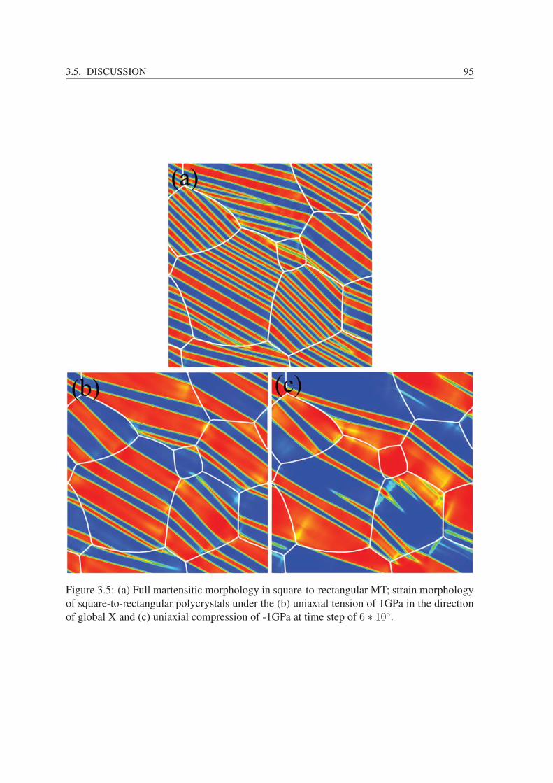
3.5. DISCUSSION 95
Figure 3.5: (a) Full martensitic morphology in square-to-rectangular MT; strain morphology
of square-to-rectangular polycrystals under the (b) uniaxial tension of 1GPa in the direction
of global X and (c) uniaxial compression of -1GPa at time step of 6 ∗ 105.

96
CHAPTER 3. NONLINEAR GINZBURG-LANDAU MODEL OF MARTENSITIC
TRANSFORMATION IN POLYCRYSTALS
Figure 3.6: (a) Full martensitic morphology in triangle-to-centered-rectangular MT; morpho-
logical evolution of polycrystalline triangle-to-centered-rectangular MT under (b)-(c) uniax-
ial tension stress of 1GPa in the direction of global X axis in a soft system with normalized
A1=9.18; and (d-e) uniaxial compression of -1GPa.

3.5. DISCUSSION 97
martensite variant (i.e. detwining, Figure 3.6c). In IRS-LR dynamics, the rebalance of the
transformation stress in system driven by the viscous term firstly develops the microstructure
into a well-formed lamellar twinning in all grains. The behaviors of variant selection diver-
sify in individual grains as the transformation strains in global coordinates differ, for specific,
in the grains with θ = π/6, the system accommodates itself by ruling out the blue variant to
form the green/red lamellar twin structure with the alignment of twin boundaries of π/3 and
5π/6, while the kinematic compatibility retains. The formation of lamellar twins is energet-
ically favored by the Level rule of thermodynamics. The direction of lamellar twin plane in
the θ = 0 grain is measured to be same as those in the θ = π/6 grain, but the dominated
twin is composed of different green and blue variants, with the red ones appear only in the
vicinity of grain boundaries. In the θ = π/12 grain, both green-blue and green-red lamellar
twins are observed with the twin boundaries along 5π/12 and 3π/4. All such alignments of
lamellar twin boundaries apparently remain to satisfy the kinematic compatibility Eq.(3.12).
The twin boundaries of the red-green variants in θ = π/6 grain rotate by π/6 with respect to
the grain orientation while those of blue-green variants in the θ = 0 grain exhibit the same
alignments as what have in single crystal. The late morphology in Figure 3.6c demonstrates
that the well-formed lamellar twins progressively give their way to the green variant at the
expense of the unfavorable red or blue twins. In one word, a long time tensile test enables
approaching a single-variant state rapidly in grains θ = 0 and π/6 while the other grains
sustain the lamellar twin structure. Thus, the green single variant martensite dominates the
microstructure with debris of isolated red or blue variants and a few lamellar twins, indi-
cating the occurrences of detwinning. Similar to the square-to-rectangular MT, a complete
single-variant microstructure is hardly obtained even after long time simulation due to the
inertia effect of LR dynamics. By monitoring the invariant plane normals for both regions of
lamellar twins and single variant martensite in Figure 3.7, the kinematic compatibility of the
austenite and martensite remains preserved in the region of lamellar twins with the directions
of π/3) in the θ = π/12 grain. However, it no longer rigidly obeys in some regions of the
detwinned single martensite.
When applying a compression up to 1 GPa to the triangle-to-centered-rectangular marten-
sites, the lamellar twins of red and blue variants fairly well present in grains with θ = π/6,
whereas the green-red twins are discovered with θ = π/24 and θ = 0, (see Figures 3.6d and
3.6e). As it evolves, the green variant tends to be suppressed, thus developing the red and
blue martensitic domains that intersect grain boundaries and exhibit coarse ’macro’ blocks or
lamella. It should be stressed that it is extremely hard to establish the grid-to-grid mapping
for the variants before and after loading since the morphology changes due to applied stress
involves complicated physical metallurgical scenarios such as the extinction and nucleation,
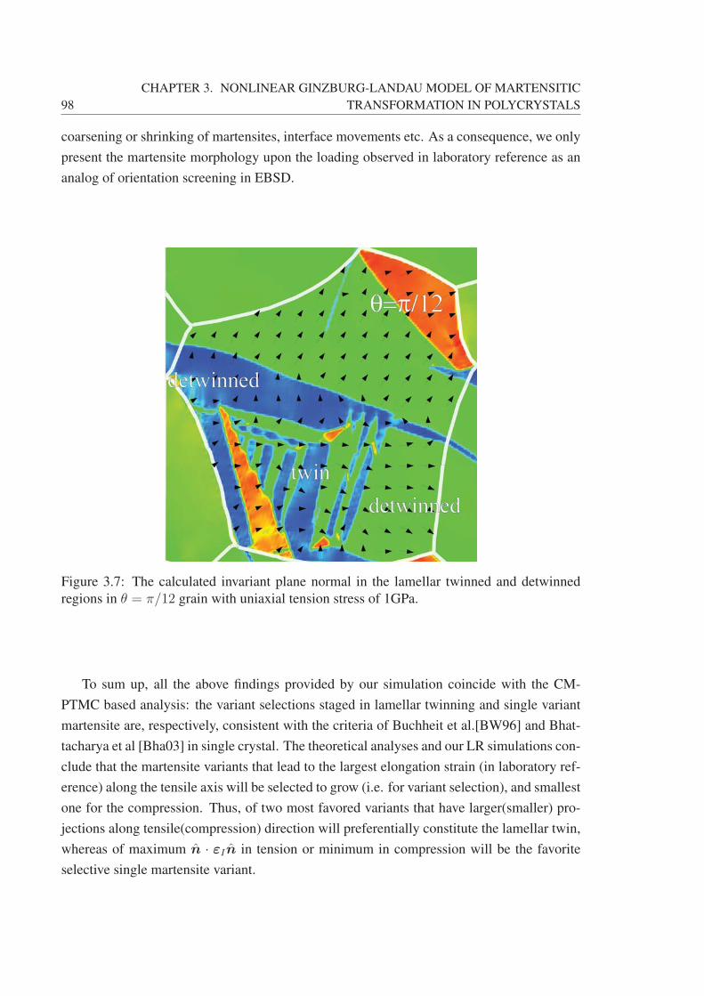
98
CHAPTER 3. NONLINEAR GINZBURG-LANDAU MODEL OF MARTENSITIC
TRANSFORMATION IN POLYCRYSTALS
coarsening or shrinking of martensites, interface movements etc. As a consequence, we only
present the martensite morphology upon the loading observed in laboratory reference as an
analog of orientation screening in EBSD.
Figure 3.7: The calculated invariant plane normal in the lamellar twinned and detwinned
regions in θ = π/12 grain with uniaxial tension stress of 1GPa.
To sum up, all the above findings provided by our simulation coincide with the CM-
PTMC based analysis: the variant selections staged in lamellar twinning and single variant
martensite are, respectively, consistent with the criteria of Buchheit et al.[BW96] and Bhat-
tacharya et al [Bha03] in single crystal. The theoretical analyses and our LR simulations con-
clude that the martensite variants that lead to the largest elongation strain (in laboratory ref-
erence) along the tensile axis will be selected to grow (i.e. for variant selection), and smallest
one for the compression. Thus, of two most favored variants that have larger(smaller) pro-
jections along tensile(compression) direction will preferentially constitute the lamellar twin,
whereas of maximum n · εIn in tension or minimum in compression will be the favorite
selective single martensite variant.
3.6. CONCLUSION 99
3.6 Conclusion
A modified model is proposed to describe the martensitic phase transformation in poly-
crystals based on the Lagrange-Rayleigh dynamics with the Landau energetics. The stress
term in the dissipative force equation is reformulated in terms of the functional of local Lan-
dau energy with respect to global displacement gradients. Through a coupling of primary
OPs to grain orientation, the model enables the description of the microstructures of MT and
elucidates its response to the external loads, with particular emphasis in the twin/habit planes
related to the crystallographic orientations and their changes. For polycrstalline square-to-
rectangular and triangle-to-centered-rectangular ferroelastic materials, the simulations re-
veal the key microstructural features found in real 3D cubic-to-tetragonal and hexagonal-
to-orthorhombic martensites, including the self-similarity of variant across grain boundaries
and the variant selection upon external loading, in agreement with what the CM-PTMC has
predicted.

100
CHAPTER 3. NONLINEAR GINZBURG-LANDAU MODEL OF MARTENSITIC
TRANSFORMATION IN POLYCRYSTALS
Chapter 4Dynamical Nucleation of Martensite inPolycrystals
The important thing in science is not so much to obtain new facts as to discover new waysof thinking about them.
-William Lawrence Bragg
4.1 Martensitic Nucleation
A preference for heterogeneous nucleation in MT has been evidenced by a wide body
of experimental explorations on steels [MXX+03, VBS09, SDC14], shape-memory alloys
[FCY+04, KADE02], ceramics [CC83, HR85], etc. The heterogeneous processes of nucle-
ation and subsequent growth at various defects present distinct microstructure [MSO+05,
BBG98], diversiform transformation pathways [Wai05, CSC+98], and hence different prop-
erties of materials [Kaj86, SJNS09]. To understand the mechanisms underlying the observed
phenomena, different theoretical studies for the nucleation of MTs have been developed
for different defects like dislocations [KC58, Chr51, OC81, RO01] and grain boundaries
[AJK02, JAK01, HC14, MABÅ13a] in perspectives of thermodynamics, kinetics and crystal
lattice dynamics. These models are at least classified into two categories considering the
classical and non-classical nucleation paths [OC82, Ols99]. The models describing classi-
cal nucleation paths believe that the embryos of martensites are formed via the dislocation
dissociation mechanism and thereafter increase in size by motion of interface. During these
processes, the nuclei have a structure and/or a composition same as those of full-formed
martensite variants, such that the driving force and kinetics of martensitic nucleation can
be discerned by evaluating the time evolution of individual energy contributions from misfit
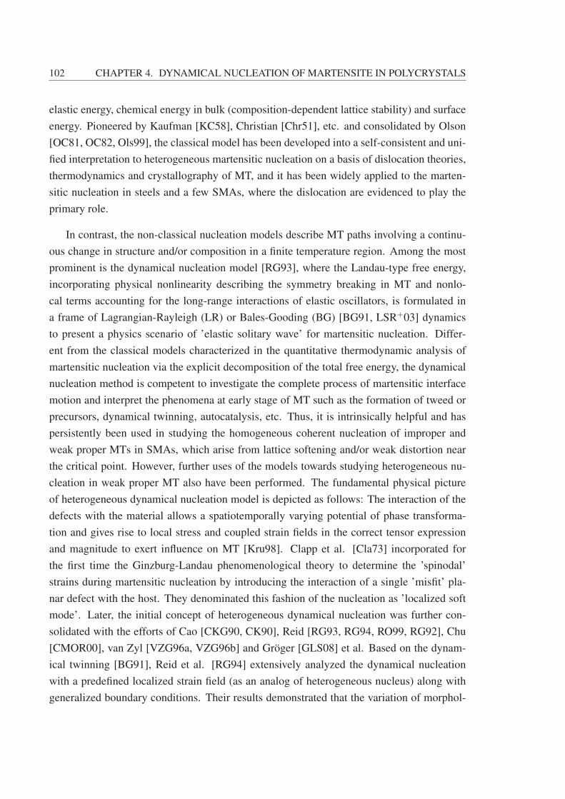
102 CHAPTER 4. DYNAMICAL NUCLEATION OF MARTENSITE IN POLYCRYSTALS
elastic energy, chemical energy in bulk (composition-dependent lattice stability) and surface
energy. Pioneered by Kaufman [KC58], Christian [Chr51], etc. and consolidated by Olson
[OC81, OC82, Ols99], the classical model has been developed into a self-consistent and uni-
fied interpretation to heterogeneous martensitic nucleation on a basis of dislocation theories,
thermodynamics and crystallography of MT, and it has been widely applied to the marten-
sitic nucleation in steels and a few SMAs, where the dislocation are evidenced to play the
primary role.
In contrast, the non-classical nucleation models describe MT paths involving a continu-
ous change in structure and/or composition in a finite temperature region. Among the most
prominent is the dynamical nucleation model [RG93], where the Landau-type free energy,
incorporating physical nonlinearity describing the symmetry breaking in MT and nonlo-
cal terms accounting for the long-range interactions of elastic oscillators, is formulated in
a frame of Lagrangian-Rayleigh (LR) or Bales-Gooding (BG) [BG91, LSR+03] dynamics
to present a physics scenario of ’elastic solitary wave’ for martensitic nucleation. Differ-
ent from the classical models characterized in the quantitative thermodynamic analysis of
martensitic nucleation via the explicit decomposition of the total free energy, the dynamical
nucleation method is competent to investigate the complete process of martensitic interface
motion and interpret the phenomena at early stage of MT such as the formation of tweed or
precursors, dynamical twinning, autocatalysis, etc. Thus, it is intrinsically helpful and has
persistently been used in studying the homogeneous coherent nucleation of improper and
weak proper MTs in SMAs, which arise from lattice softening and/or weak distortion near
the critical point. However, further uses of the models towards studying heterogeneous nu-
cleation in weak proper MT also have been performed. The fundamental physical picture
of heterogeneous dynamical nucleation model is depicted as follows: The interaction of the
defects with the material allows a spatiotemporally varying potential of phase transforma-
tion and gives rise to local stress and coupled strain fields in the correct tensor expression
and magnitude to exert influence on MT [Kru98]. Clapp et al. [Cla73] incorporated for
the first time the Ginzburg-Landau phenomenological theory to determine the ’spinodal’
strains during martensitic nucleation by introducing the interaction of a single ’misfit’ pla-
nar defect with the host. They denominated this fashion of the nucleation as ’localized soft
mode’. Later, the initial concept of heterogeneous dynamical nucleation was further con-
solidated with the efforts of Cao [CKG90, CK90], Reid [RG93, RG94, RO99, RG92], Chu
[CMOR00], van Zyl [VZG96a, VZG96b] and Gröger [GLS08] et al. Based on the dynam-
ical twinning [BG91], Reid et al. [RG94] extensively analyzed the dynamical nucleation
with a predefined localized strain field (as an analog of heterogeneous nucleus) along with
generalized boundary conditions. Their results demonstrated that the variation of morphol-
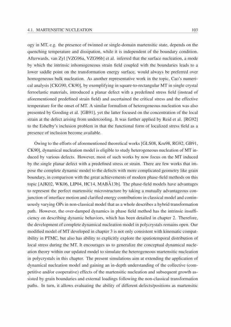
4.1. MARTENSITIC NUCLEATION 103
ogy in MT, e.g. the presence of twinned or single-domain martensitic state, depends on the
quenching temperature and dissipation, while it is independent of the boundary condition.
Afterwards, van Zyl [VZG96a, VZG96b] et al. inferred that the surface nucleation, a mode
by which the intrinsic inhomogeneous strain field coupled with the boundaries leads to a
lower saddle point on the transformation energy surface, would always be preferred over
homogeneous bulk nucleation. As another representative work in the topic, Cao’s numeri-
cal analysis [CKG90, CK90], by exemplifying in square-to-rectangular MT in single crystal
ferroelastic materials, introduced a planar defect with a predefined stress field (instead of
aforementioned predefined strain field) and ascertained the critical stress and the effective
temperature for the onset of MT. A similar formalism of heterogeneous nucleation was also
presented by Gooding et al. [GB91], yet the latter focused on the concentration of the local
strain at the defect arising from undercooling. It was further applied by Reid et al. [RG92]
to the Eshelby’s inclusion problem in that the functional form of localized stress field as a
presence of inclusion become available.
Owing to the efforts of aforementioned theoretical works [GLS08, Kru98, RG92, GB91,
CK90], dynamical nucleation model is eligible to study heterogeneous nucleation of MT in-
duced by various defects. However, most of such works by now focus on the MT induced
by the single planar defect with a predefined stress or strain. There are few works that im-
pose the complete dynamic model to the defects with more complicated geometry like grain
boundary, in comparison with the great achievements of modern phase-field methods on this
topic [AJK02, WK06, LIP04, HC14, MABÅ13b]. The phase-field models have advantages
to represent the perfect martensitic microstructure by taking a mutually advantageous con-
junction of interface motion and clarified energy contributions in classical model and contin-
uously varying OPs in non-classical model that as a whole describes a hybrid transformation
path. However, the over-damped dynamics in phase field method has the intrinsic insuffi-
ciency on describing dynamic behaviors, which has been detailed in chapter 2. Therefore,
the development of complete dynamical nucleation model in polycrystals remains open. Our
modified model of MT developed in chapter 3 is not only consistent with kinematic compat-
ibility in PTMC, but also has ability to explicitly explore the spatiotemporal distribution of
local stress during the MT. It encourages us to generalize the conceptual dynamical nucle-
ation theory within our updated model to simulate the heterogeneous martensitic nucleation
in polycrystals in this chapter. The present simulations aim at extending the application of
dynamical nucleation model and gaining an in-depth understanding of the collective (com-
petitive and/or cooperative) effects of the martensitic nucleation and subsequent growth as-
sisted by grain boundaries and external loadings following the non-classical transformation
paths. In turn, it allows evaluating the ability of different defects/positions as martensitic

104 CHAPTER 4. DYNAMICAL NUCLEATION OF MARTENSITE IN POLYCRYSTALS
nucleation sites originating from the interaction of intrinsic polycrystalline defects with the
applied loading in a weak proper MT.
4.2 Dynamical Nucleation Model in Polycrystals
The dynamical nucleation of MT induced by grain boundary in a polycrystal can be
achieved once the predefined planar defects in Refs. [CKG90, CK90, GB91] are specified
as the grain boundaries and triple junctions. Rather than considering an inhomogeneous
stress field explicitly induced by the defects [CKG90, CK90], we make an effort to study
what effects may produce during MT when the uniaxial tensile loading interacts with grain
boundary. The grain boundaries can perceive the applied stress and feel back to couple with
Landau transformation potential, thereafter, lead to a localized stress field and modify the
transformation temperature. Similar to Cao’s work on single crystal [CKG90], we assume
that 1) the inhomogeneous distribution of stress is produced by defects, specifically in this
work, the localized stress fields around the grain boundaries and triple junctions, rather than
the defects themselves; 2) the interface between austenite and martensite is coherent which is
imposed by the compatibility condition; 3) the displacement at grain boundary is continuous
as required by the displacement-based Lagrange-Rayleigh dynamics [LSR+03] . It infers
that free surfaces and incoherent grain boundaries are not taken into consideration. It is also
noted that we are not intending to obtain various morphology by mediating the damping
parameters as what conventional dynamical nucleation modeling did, rather, we focus on
how intrinsic MT potential involving with grain boundaries and applied stresses leads to
different nucleation modes or sites.
In this chapter, the Fe-Pd alloy is still adopted to exemplify our dynamical nucleation
model. The Landau free energy and dynamic equations in this chapter are same as those in
chapter 3. The only difference is that the simple uniaxial stress is exerted at the initial stage
of simulation and does effects on martensitic nucleation. The free energy contribution due
to the applied stress σapp can be yielded as
fapp = −σappexx (4.1)
Thus, the free energy is finally expressed in global coordinates as
F =
∫dr
⎡⎣ A1
2e21(r, θ)+
A20
2
(T − Tc
Ms − Tc
)e22(r, θ) +
A4
4e42(r, θ) +
A6
6e62(r, θ)+
A3
2e23(r, θ)
+g(∇e2(r, θ))2 + fgrains (θ)− σappexx (r, θ)
⎤⎦
(4.2)

4.3. MICROSTRUCTURE EVOLUTION 105
The materials parameters were exactly same as those in chapter 3. During the simu-
lations, the different external stresses were applied to the simulation box. The simulation
results are discussed in the following paragraphs.
4.3 Microstructure Evolution
The martensitic nucleation and the relevant microstructure evolution are studied by the
simulations under the conditions of (1) different applied stresses at a fixed temperature, (2)
different temperatures with a constant applied stress, and (3) the combination of varying
stresses and temperatures. These external processing conditions interacting with intrinsic
MT energy lead to different scenarios of martensitic nucleation.
4.3.1 Heterogeneous Nucleation under the Applied Stressof 50 MPa
To examine the martensitic nucleation in the vicinity of grain boundaries, the system
was first quenched to T = 275K (Tc < T < Ms), followed by an isothermal simulation
under a constant applied stress of σapp = 50MPa. The setting temperature, slightly higher
than Tc, ensures the existence of an energy barrier to describe the nature of first-order MT
yet allows a small thermal activation to jump over. The sequential process of the nucle-
ation and growth of the martensite is shown in Figure 4.1, where the martensite is depicted
by distribution of the deviatoric strain e2 at different times during the isothermal simula-
tion. The thermal fluctuations give rise to local inhomogeneity of the deviatoric strain at the
initial stage of the isothermal simulation that trigger the onset of a fine-scale assembly of
cross-hatched tweeds (Figure 4.1-b). Differing from single crystals [KKSW95], the tweeds
exhibit different stretch directions in individual grains. Note that tweeds similar to those in
Figure 4.1b can also develop above Ms in the absence of the applied stress. There is local
distortion of deviatoric strain caused by the localized stress field accumulating at the grain
boundaries with larger misorientation, as those between blue and red grains in Figure 4.1b.
It indicates that the free energy minima have been momentarily shifted toward the grain
boundaries due to the synergistic contribution of the grain boundary energy and the strain
gradients. For σapp = 50MPa, no concentration of deviatoric strain is found in the vicinity
of triple junctions because the superposition of strain gradients stemming from individual
grain boundaries leads to a relatively more homogeneous strain field at the triple junction.
The fine tweeds inside the grains and deviatoric strain distortion at grain boundaries are fad-
ing away with time, and the system subjected to σapp = 50MPa responds to the localized
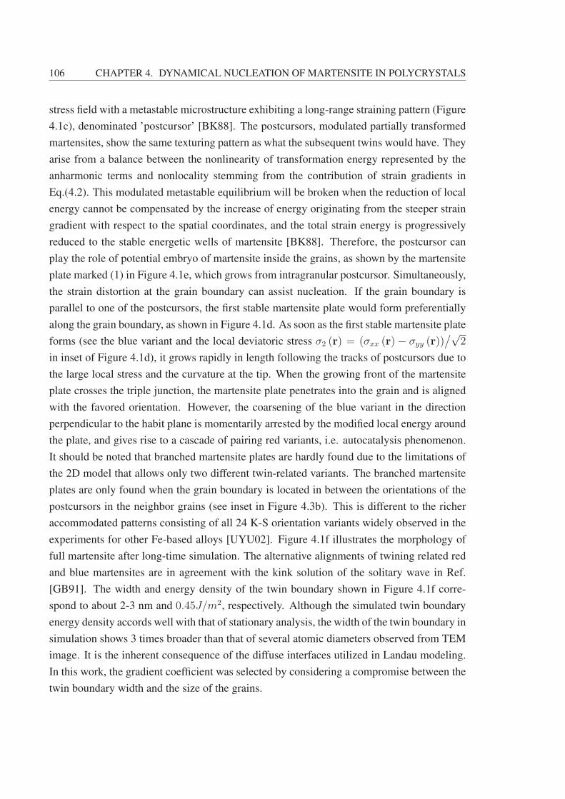
106 CHAPTER 4. DYNAMICAL NUCLEATION OF MARTENSITE IN POLYCRYSTALS
stress field with a metastable microstructure exhibiting a long-range straining pattern (Figure
4.1c), denominated ’postcursor’ [BK88]. The postcursors, modulated partially transformed
martensites, show the same texturing pattern as what the subsequent twins would have. They
arise from a balance between the nonlinearity of transformation energy represented by the
anharmonic terms and nonlocality stemming from the contribution of strain gradients in
Eq.(4.2). This modulated metastable equilibrium will be broken when the reduction of local
energy cannot be compensated by the increase of energy originating from the steeper strain
gradient with respect to the spatial coordinates, and the total strain energy is progressively
reduced to the stable energetic wells of martensite [BK88]. Therefore, the postcursor can
play the role of potential embryo of martensite inside the grains, as shown by the martensite
plate marked (1) in Figure 4.1e, which grows from intragranular postcursor. Simultaneously,
the strain distortion at the grain boundary can assist nucleation. If the grain boundary is
parallel to one of the postcursors, the first stable martensite plate would form preferentially
along the grain boundary, as shown in Figure 4.1d. As soon as the first stable martensite plate
forms (see the blue variant and the local deviatoric stress σ2 (r) = (σxx (r)− σyy (r))/√
2
in inset of Figure 4.1d), it grows rapidly in length following the tracks of postcursors due to
the large local stress and the curvature at the tip. When the growing front of the martensite
plate crosses the triple junction, the martensite plate penetrates into the grain and is aligned
with the favored orientation. However, the coarsening of the blue variant in the direction
perpendicular to the habit plane is momentarily arrested by the modified local energy around
the plate, and gives rise to a cascade of pairing red variants, i.e. autocatalysis phenomenon.
It should be noted that branched martensite plates are hardly found due to the limitations of
the 2D model that allows only two different twin-related variants. The branched martensite
plates are only found when the grain boundary is located in between the orientations of the
postcursors in the neighbor grains (see inset in Figure 4.3b). This is different to the richer
accommodated patterns consisting of all 24 K-S orientation variants widely observed in the
experiments for other Fe-based alloys [UYU02]. Figure 4.1f illustrates the morphology of
full martensite after long-time simulation. The alternative alignments of twining related red
and blue martensites are in agreement with the kink solution of the solitary wave in Ref.
[GB91]. The width and energy density of the twin boundary shown in Figure 4.1f corre-
spond to about 2-3 nm and 0.45J/m2, respectively. Although the simulated twin boundary
energy density accords well with that of stationary analysis, the width of the twin boundary in
simulation shows 3 times broader than that of several atomic diameters observed from TEM
image. It is the inherent consequence of the diffuse interfaces utilized in Landau modeling.
In this work, the gradient coefficient was selected by considering a compromise between the
twin boundary width and the size of the grains.

4.3. MICROSTRUCTURE EVOLUTION 107
Figure 4.1: (a) Spatial distribution of the grain orientation angle as indicated in each grain
(b)-(f) Martensitic nucleation and growth in polycrystals, as shown by the deviatoric strain e2at 275K under an applied stress σapp = 50MPa, at time steps of 800, 12000, 92000, 94800
and 104000, respectively. The red and blue domains represent two martensite variants while
the green domain is austenite. The grain boundaries are displayed in white.
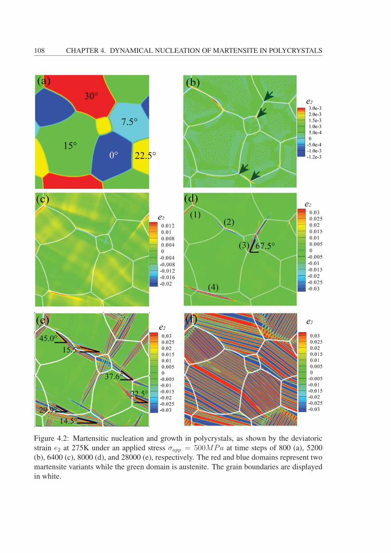
108 CHAPTER 4. DYNAMICAL NUCLEATION OF MARTENSITE IN POLYCRYSTALS
Figure 4.2: Martensitic nucleation and growth in polycrystals, as shown by the deviatoric
strain e2 at 275K under an applied stress σapp = 500MPa at time steps of 800 (a), 5200
(b), 6400 (c), 8000 (d), and 28000 (e), respectively. The red and blue domains represent two
martensite variants while the green domain is austenite. The grain boundaries are displayed
in white.

4.3. MICROSTRUCTURE EVOLUTION 109
4.3.2 Heterogeneous Nucleation under the Applied Stressof 500 MPa
The martensitic nucleation under σapp = 500MPa shows similar features (Figure 4.2b)
at the early stages of the simulation: the tweed pattern develops within the grains and strain
distortions appear at grain boundaries, but both occur more rapidly because of the higher
stresses. The accumulation of the deviatoric strain raised by the local stress is supposed to
smear out or weaken the effect of postcursors. At the same time, the interplaying of elas-
tic transformation energy and lattice curvature drives the ’twinned’ strain distortion to split
into ’diploes’ (indicated by the arrows in Figure 4.2-b) and be located at the triple junctions
and high angle grain boundaries, both of which serve as the preferential sites for martensitic
nucleation and growth, as shown in Figure 4.2c. Three martensite plates (marked (1), (2)
and (3) in Figure 4.2d) are nucleated at the triple junctions, and grow into the twins aligned
with their optimum twinning orientations in individual grains. For instance, the pairs of
needle-like martensites in the grains with the orientation θ = 22.5◦ (i.e. the grains in yellow
in Figure 4.2a) align along the 67.5◦ with respect to the horizontal axis of global reference.
A different scenario is found in the twinned martensite plates marked (4) in Figure 4.2d.
They nucleate and grow assisted by the high angle grain boundaries, and the leading plate in
red propagates beyond the neighbor triple junction without changing orientation apparently.
However, it accommodates itself later to match the surrounding grain misorientation by sub-
tly rotating the residing twin boundary to form the full martensitic morphology (Figure 4.2f).
4.3.3 The Effect of Applied Stress on Heterogeneous Nu-cleation at Grain Boundaries
In Figure 4.3, the deviatoric strain as a function of the distance to a high angle grain
boundary is plotted for different applied stresses and times at T = 275K. Although the
high angle grain boundaries can be considered analogous to 2D planar defects in Refs.
[CK90, GB91], we must clarify that our modeling has its root in the dynamical nucleation de-
veloped by Clapp [Cla93],Cao [CKG90, CK90] and Gooding et al. [GB91] The hyperbolic-
type profiles of the deviatoric strain are consistent with the analytical results of Cao [CK90]
who introduced a predefined stress field as a martensite embryo for twin. The deviatoric
strains raised by the small local stresses rapidly accumulate within the first hundreds of steps
(see inset of Figure 4.3 with σapp = 20 − 100MPa). However, they are one to two orders
of magnitude smaller than the threshold of ’spinodal strain’ to serve as steady martensite
embryos or form stable martensite variants. The strain profile with σapp = 500MPa and at
normalized time t∗ = 6400 (in the direction perpendicular to the twin plane 4# in Figure
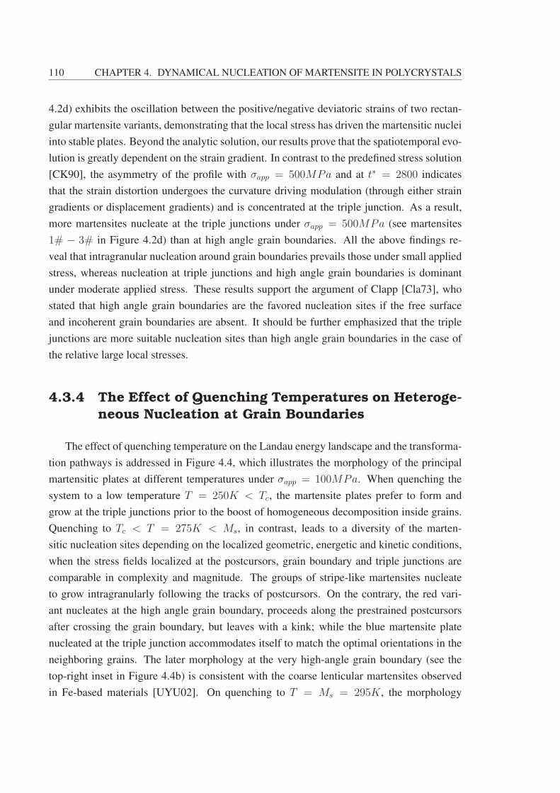
110 CHAPTER 4. DYNAMICAL NUCLEATION OF MARTENSITE IN POLYCRYSTALS
4.2d) exhibits the oscillation between the positive/negative deviatoric strains of two rectan-
gular martensite variants, demonstrating that the local stress has driven the martensitic nuclei
into stable plates. Beyond the analytic solution, our results prove that the spatiotemporal evo-
lution is greatly dependent on the strain gradient. In contrast to the predefined stress solution
[CK90], the asymmetry of the profile with σapp = 500MPa and at t∗ = 2800 indicates
that the strain distortion undergoes the curvature driving modulation (through either strain
gradients or displacement gradients) and is concentrated at the triple junction. As a result,
more martensites nucleate at the triple junctions under σapp = 500MPa (see martensites
1# − 3# in Figure 4.2d) than at high angle grain boundaries. All the above findings re-
veal that intragranular nucleation around grain boundaries prevails those under small applied
stress, whereas nucleation at triple junctions and high angle grain boundaries is dominant
under moderate applied stress. These results support the argument of Clapp [Cla73], who
stated that high angle grain boundaries are the favored nucleation sites if the free surface
and incoherent grain boundaries are absent. It should be further emphasized that the triple
junctions are more suitable nucleation sites than high angle grain boundaries in the case of
the relative large local stresses.
4.3.4 The Effect of Quenching Temperatures on Heteroge-neous Nucleation at Grain Boundaries
The effect of quenching temperature on the Landau energy landscape and the transforma-
tion pathways is addressed in Figure 4.4, which illustrates the morphology of the principal
martensitic plates at different temperatures under σapp = 100MPa. When quenching the
system to a low temperature T = 250K < Tc, the martensite plates prefer to form and
grow at the triple junctions prior to the boost of homogeneous decomposition inside grains.
Quenching to Tc < T = 275K < Ms, in contrast, leads to a diversity of the marten-
sitic nucleation sites depending on the localized geometric, energetic and kinetic conditions,
when the stress fields localized at the postcursors, grain boundary and triple junctions are
comparable in complexity and magnitude. The groups of stripe-like martensites nucleate
to grow intragranularly following the tracks of postcursors. On the contrary, the red vari-
ant nucleates at the high angle grain boundary, proceeds along the prestrained postcursors
after crossing the grain boundary, but leaves with a kink; while the blue martensite plate
nucleated at the triple junction accommodates itself to match the optimal orientations in the
neighboring grains. The later morphology at the very high-angle grain boundary (see the
top-right inset in Figure 4.4b) is consistent with the coarse lenticular martensites observed
in Fe-based materials [UYU02]. On quenching to T = Ms = 295K, the morphology
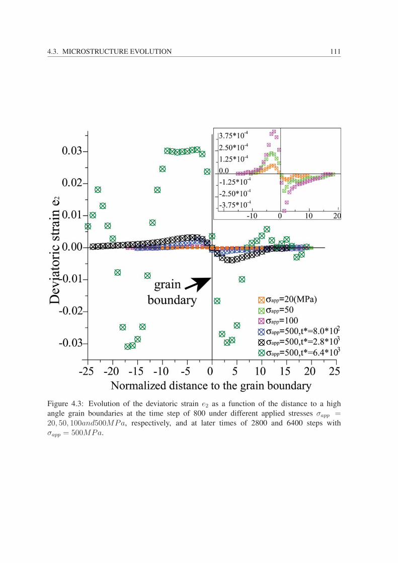
4.3. MICROSTRUCTURE EVOLUTION 111
Figure 4.3: Evolution of the deviatoric strain e2 as a function of the distance to a high
angle grain boundaries at the time step of 800 under different applied stresses σapp =20, 50, 100and500MPa, respectively, and at later times of 2800 and 6400 steps with
σapp = 500MPa.

112 CHAPTER 4. DYNAMICAL NUCLEATION OF MARTENSITE IN POLYCRYSTALS
exhibits a heterogeneous structure containing austenite-martensite alternated stripes in the
grains (Figure 4.4c). This process takes place via the nucleation and growth relying on the
preexisting postcursors with a morphology much like the stress-induced martensite at room
temperature (T > Ms) for certain cubic-to-monoclinic II SMAs [US13]. Note that since the
symmetry breaking of cubic-to-monoclinic II transformation contains the elements of cubic-
to-tretragonal one, a specific 2D projection of the microstructure of cubic-to-monoclinic II
in a fine wire sample could sustain the lamella features in tetragonal alloys [LXC14]. The
formation of a single martensite variant in equilibrium with the austenite is energetically
allowed at Ms, and even at higher temperature, if the local stress is above a threshold. Nev-
ertheless, it is constrained by geometrical compatibility in 3D bulk materials. So far, our
simulations have demonstrated that the martensitic nucleation modes (sites) are sensitive to
the quenching temperature. The primary nucleation sites vary from triple junctions to high
angle grain boundaries to postcursors as the quenching temperature increases. Thus, it can
be inferred that a continuous cooling to a lower temperature is perfectly adequate to yield
the formation of stable martensite plates at the triple junctions, as proven in Figure 4.4d.
4.3.5 Phase Diagram of Nucleation Modes
Most of the discoveries by our simulations can be summarized in the phase diagram of
nucleation modes for the Fe-Pd ferroelastics presented in Figure 4.5. The phase diagram
has a look similar to a conventional TTT diagram, and conveys the information about the
principally favored mode of martensitic nucleation under particular combination of quench-
ing temperature and applied stress. It is still noteworthy that the nucleation and growth of
martensite are actually governed by the local stress rather than by the applied stress. How-
ever, the applied stresses can be easily used to control processing in an industrial environ-
ment. The phase diagram manifests that nucleation at the postcursors dominates at high
quenching temperatures. As the quenching temperature decreases or the applied stress in-
creases, nucleation at the postcursors is replaced by four distinct mixed modes, namely, grain
boundary + postcursor, triple junction + postcursor, hybrid (i.e. all sorts of nucleation sites
are possible) and triple junction + grain boundary. Only the postcursors can develop them-
selves to a type of nucleation sites, while the grain boundaries and triple junctions have to
cooperate to become viable nucleation sites, as shown in Figure 4.5. It is worth pointing out
that our results have been obtained assuming that the material was elastic and continuous.
Thus, other aspects associated with grain boundary nucleation such as plasticity, incoher-
ent interfaces and defect cores have not been considered. The incorporation of these issues
into the simulation will be necessary to include more physics in the model and enhance the
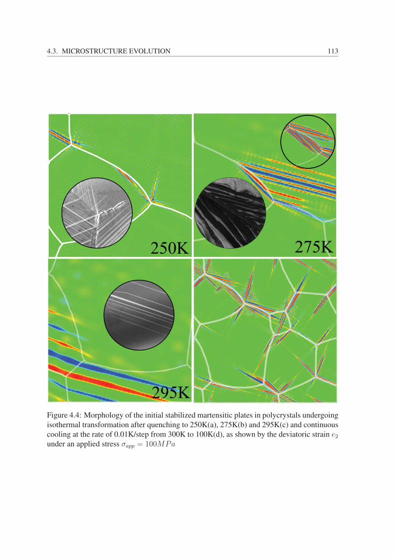
4.3. MICROSTRUCTURE EVOLUTION 113
Figure 4.4: Morphology of the initial stabilized martensitic plates in polycrystals undergoing
isothermal transformation after quenching to 250K(a), 275K(b) and 295K(c) and continuous
cooling at the rate of 0.01K/step from 300K to 100K(d), as shown by the deviatoric strain e2under an applied stress σapp = 100MPa
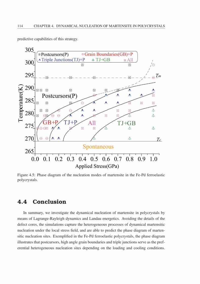
114 CHAPTER 4. DYNAMICAL NUCLEATION OF MARTENSITE IN POLYCRYSTALS
predictive capabilities of this strategy.
Figure 4.5: Phase diagram of the nucleation modes of martensite in the Fe-Pd ferroelastic
polycrystals.
4.4 Conclusion
In summary, we investigate the dynamical nucleation of martensite in polycrystals by
means of Lagrange-Rayleigh dynamics and Landau energetics. Avoiding the details of the
defect cores, the simulations capture the heterogeneous processes of dynamical martensitic
nucleation under the local stress field, and are able to predict the phase diagram of marten-
sitic nucleation sites. Exemplified in the Fe-Pd ferroelastic polycrystals, the phase diagram
illustrates that postcursors, high angle grain boundaries and triple junctions serve as the pref-
erential heterogeneous nucleation sites depending on the loading and cooling conditions.

4.4. CONCLUSION 115
The information, presented in the form of a phase diagram like Figure 4.5, specify how the
quenching temperature and applied stress conditions can be combined to activate particular
mechanisms of martensitic nucleation and growth, leading to complex microstructures in
order to meet microstructural design goals.

116 CHAPTER 4. DYNAMICAL NUCLEATION OF MARTENSITE IN POLYCRYSTALS

Chapter 5Displacive-Diffusive Model Integratedwith CALPHAD Technique
Metallographic information is still a basis for interpreting and modeling variousphenomena and metallography provides an important testing ground for models.
-Mats Hillert 1999
Quantitative Landau modeling coupled with computational thermo-kinetics is capable
of simulating microstructure evolution over the arrays of composition, heat treatment and
processing. It opens up a new way of prediction and control of microstructure and properties,
by doing so, upgrades the traditional ’trial-error’ method towards orientated alloys design.
5.1 CALPHAD and Computational Thermodynam-ics
The microstructure development in a real processing is always influenced by the coop-
eration and/or competition between displacive and diffusional transformations. Despite the
physics robustness of Landau theory in modeling many displacive phase transformations in
solids, it should be coupled with other advanced techniques in order to predict the microstruc-
ture evolution in real alloy systems subjected to real processing [Ste09, GBTF00]. To quan-
titatively (or semi quantitatively) control the microstructure, the precise thermodynamic and
kinetic inputs are vital to a Landau simulation for displacive-diffusive coupled phase trans-
formation [ZSD+15]. In contrast to Landau polynomial served as grand potential in theoret-
ical analysis, the Gibbs energy is widely applied for engineering use, because both tempera-
ture and pressure, as independent thermodynamic variables of Gibbs energy, can be feasibly

118
CHAPTER 5. DISPLACIVE-DIFFUSIVE MODEL INTEGRATED WITH CALPHAD
TECHNIQUE
controlled in industry. Among various integration of models at different scales for the (semi-
) quantitative simulation, the phase field modeling coupled with CALPHAD (Calculation of
PHAse Diagram) technique has acheived great success [CMWW04, WZP+08, EBS06]. The
CALPHAD technique is a sub-discipline of computational materials science [Xio15]. By si-
multaneously evaluating thermochemistry properties of each phase and information of phase
diagram to obtain database with mathematical models containing self-consistent parameters,
the CALPHAD technique provides reliable thermodynamic data and phase diagram informa-
tion for practical processes and helps to get deeper insights into the physical metallurgical
mechanisms of the materials behaviors via computer calculation/simulation.
The scientific foundation of CALPHAD technique is that a phase diagram manifests the
equilibrium thermodynamic properties of the system. Various thermodynamic variables can
be expressed as functional of the Gibbs energy of the system and/or individual phases. Al-
though several earlier works of binary and ternary phase diagrams had been glittering with
the wisdom of Van Laar [VL08], Wagner [WMW52], Meijering [Mei59], Kubaschewski
[OC65], et al., the representation of phase diagram of multicomponent and multiphase sys-
tem and the prediction of thermodynamic properties in a space of complicated processing
variables by ’hand construction’ was undoubtedly a nightmare before the prevailing of com-
puter simulations. Initiated by Kaufman [KRSJ67] and Ansara [ABKS78] who introduced
the concept of lattice stability in calculating phase diagrams and consolidated by Hillert’s
effort on the comprehensive thermodynamic theories of phase diagram, phase equilibria
and phase transformation [Hil80, Hil07], significant advances of CALPHAD technique have
been achieved over the past decades, including the design of high efficient algorithm and
robust software to optimize and derive thermodynamic parameters, proposition of thermody-
namic reasonable models, assessment of self-consistent databases for multicomponent sys-
tems, and tons of calculations upon powerful computing engine and databanks to improve
understanding of various industrial and technological processes. Served as the roadmap for
materials research, CALPHAD technique helped to discover the cobalt based super alloy
[SOO+06], select the most promising composition candidates for lead-free solders [ZT02],
accelerate the data mining of new generation of databanks extending from conventional ther-
modynamic properties to all physics properties and so forth. Nowadays CALPHAD tech-
nique has gained rebirth with the name of Computational Thermodynamics and has made a
major breakthrough being considered as one of the most successful tools for materials de-
sign and acted as core fundamental infrastructure for Integrated Computational Materials
Engineering (ICME) [SP12] to integrate with other computational techniques such as first
principles calculations, phase field modeling, molecular dynamic simulations and so on.
In this chapter, the strategic work that couples CALPHAD technique with Landau model

5.2. THERMO-KINETIC MODEL IN CALPHAD TECHNIQUE 119
is devoted. More specific, the Compound Energy Formalism (CEF) [Hil01, LFS07] based
Gibbs energy and atomic diffusion mobility models for diffusive transformation are incor-
porated to IRS based Landau model developed in previous chapters for displacive transfor-
mation. In the sections follow, the integrated model is applied to the simulations of mi-
crostructure and composition evolution in hypothetical dislocation-free steels resulting from
the Quenching and Partitioning(Q&P) process.
5.2 Thermo-Kinetic Model in CALPHAD Technique
Different from the energy expression in Landau model and most of phase field models
(except for the multi-phase-field model), the Gibbs energy is individually modeled for each
phase in CALPHAD technique and the total Gibbs energy of a system is expressed as the
phase fraction weighted summation of Gibbs energy of individual phases, i.e.
Gsystem =
∑θ
φθGθ. (5.1)
The φθ and Gθ are phase fraction and Gibbs energy of θ phase, respectively. The Gibbs
energy of a phase, Gθ, is an extensive property, depending on the amounts of the constituents
in the phase. In CALPHAD community, modeling a composition dependent property is more
convenient to use the molar Gibbs energy, Gm, defined in Eq. (5.2), and gives the size of the
system as the total amount of components, N , which is the sum of moles of all components
Ni
Gθ = NG
θm, N =
∑i
Ni, xci =∑i
Ni
/N. (5.2)
In general, the molar Gibbs energy of a phase is expressed as
Gθm = G
θm
srf +Gθm
id +Gθm
ex +Gθm
phys (5.3)
where the superscript srf stands for ’surface of reference’. This term represents the Gibbs
energy of an unreacted mechanical mixture of the end-member species. The temperature de-
pendence of the molar Gibbs energy of each end-member phase (pure substance or stoichio-
metric compound) relative to a selected reference state (conventionally the room temperature
298.15K and 1atm) is derived from the Kirchhoff’s law of heat capacity, and described by a
power series
Gθ◦m = G
θ−SER◦m + a+ bT + cT lnT + dT 2 + eT−1 + fT 3... (5.4)
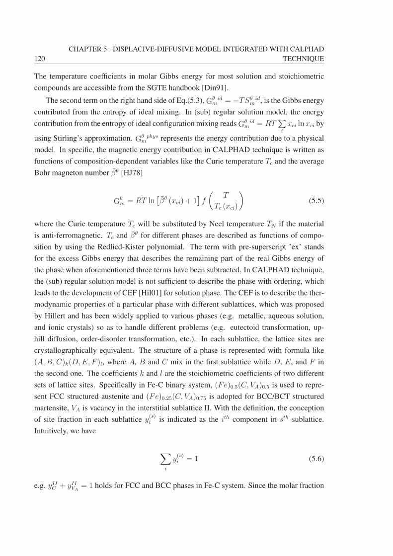
120
CHAPTER 5. DISPLACIVE-DIFFUSIVE MODEL INTEGRATED WITH CALPHAD
TECHNIQUE
The temperature coefficients in molar Gibbs energy for most solution and stoichiometric
compounds are accessible from the SGTE handbook [Din91].
The second term on the right hand side of Eq.(5.3), Gθm
id = −TSθm
id, is the Gibbs energy
contributed from the entropy of ideal mixing. In (sub) regular solution model, the energy
contribution from the entropy of ideal configuration mixing reads Gθm
id = RT∑i
xci ln xci by
using Stirling’s approximation. Gθm
phys represents the energy contribution due to a physical
model. In specific, the magnetic energy contribution in CALPHAD technique is written as
functions of composition-dependent variables like the Curie temperature Tc and the average
Bohr magneton number βθ [HJ78]
Gθm = RT ln
[βθ (xci) + 1
]f
(T
Tc (xci)
)(5.5)
where the Curie temperature Tc will be substituted by Neel temperature TN if the material
is anti-ferromagnetic. Tc and βθ for different phases are described as functions of compo-
sition by using the Redlicd-Kister polynomial. The term with pre-superscript ’ex’ stands
for the excess Gibbs energy that describes the remaining part of the real Gibbs energy of
the phase when aforementioned three terms have been subtracted. In CALPHAD technique,
the (sub) regular solution model is not sufficient to describe the phase with ordering, which
leads to the development of CEF [Hil01] for solution phase. The CEF is to describe the ther-
modynamic properties of a particular phase with different sublattices, which was proposed
by Hillert and has been widely applied to various phases (e.g. metallic, aqueous solution,
and ionic crystals) so as to handle different problems (e.g. eutectoid transformation, up-
hill diffusion, order-disorder transformation, etc.). In each sublattice, the lattice sites are
crystallographically equivalent. The structure of a phase is represented with formula like
(A,B,C)k(D,E, F )l, where A, B and C mix in the first sublattice while D, E, and F in
the second one. The coefficients k and l are the stoichiometric coefficients of two different
sets of lattice sites. Specifically in Fe-C binary system, (Fe)0.5(C, VA)0.5 is used to repre-
sent FCC structured austenite and (Fe)0.25(C, VA)0.75 is adopted for BCC/BCT structured
martensite, VA is vacancy in the interstitial sublattice II. With the definition, the conception
of site fraction in each sublattice y(s)i is indicated as the ith component in sth sublattice.
Intuitively, we have
∑i
y(s)i = 1 (5.6)
e.g. yIIC + yIIVA= 1 holds for FCC and BCC phases in Fe-C system. Since the molar fraction
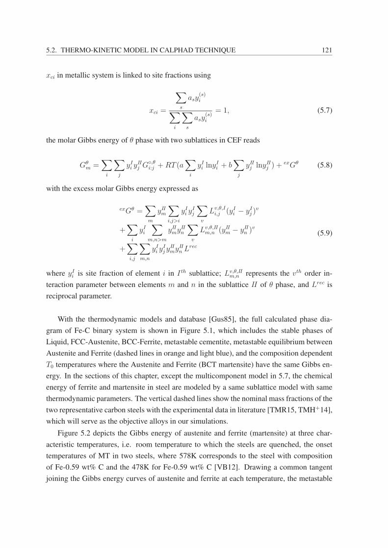
5.2. THERMO-KINETIC MODEL IN CALPHAD TECHNIQUE 121
xci in metallic system is linked to site fractions using
xci =
∑s
asy(s)i∑
i
∑s
asy(s)i
= 1, (5.7)
the molar Gibbs energy of θ phase with two sublattices in CEF reads
Gθm =
∑i
∑j
yIi yIIj G
◦,θi:j +RT (a
∑i
yIi lnyIi + b
∑j
yIIj lnyIIj ) +exGθ (5.8)
with the excess molar Gibbs energy expressed as
exGθ =∑m
yIIm∑i,j>i
yIi yIj
∑v
Lv,θ,Ii,j (yIi − yIj )
v
+∑i
yIi∑
m,n>m
yIImyIIn
∑v
Lv,θ,IIm,n (yIIm − yIIn )
v
+∑i,j
∑m,n
yIi yIj y
IImy
IIn L
rec
(5.9)
where yIi is site fraction of element i in I th sublattice; Lv,θ,IIm,n represents the vth order in-
teraction parameter between elements m and n in the sublattice II of θ phase, and Lrec is
reciprocal parameter.
With the thermodynamic models and database [Gus85], the full calculated phase dia-
gram of Fe-C binary system is shown in Figure 5.1, which includes the stable phases of
Liquid, FCC-Austenite, BCC-Ferrite, metastable cementite, metastable equilibrium between
Austenite and Ferrite (dashed lines in orange and light blue), and the composition dependent
T0 temperatures where the Austenite and Ferrite (BCT martensite) have the same Gibbs en-
ergy. In the sections of this chapter, except the multicomponent model in 5.7, the chemical
energy of ferrite and martensite in steel are modeled by a same sublattice model with same
thermodynamic parameters. The vertical dashed lines show the nominal mass fractions of the
two representative carbon steels with the experimental data in literature [TMR15, TMH+14],
which will serve as the objective alloys in our simulations.
Figure 5.2 depicts the Gibbs energy of austenite and ferrite (martensite) at three char-
acteristic temperatures, i.e. room temperature to which the steels are quenched, the onset
temperatures of MT in two steels, where 578K corresponds to the steel with composition
of Fe-0.59 wt% C and the 478K for Fe-0.59 wt% C [VB12]. Drawing a common tangent
joining the Gibbs energy curves of austenite and ferrite at each temperature, the metastable
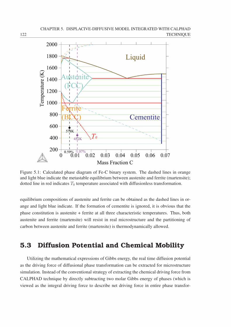
122
CHAPTER 5. DISPLACIVE-DIFFUSIVE MODEL INTEGRATED WITH CALPHAD
TECHNIQUE
Figure 5.1: Calculated phase diagram of Fe-C binary system. The dashed lines in orange
and light blue indicate the metastable equilibrium between austenite and ferrite (martensite);
dotted line in red indicates T0 temperature associated with diffusionless transformation.
equilibrium compositions of austenite and ferrite can be obtained as the dashed lines in or-
ange and light blue indicate. If the formation of cementite is ignored, it is obvious that the
phase constitution is austenite + ferrite at all three characteristic temperatures. Thus, both
austenite and ferrite (martensite) will resist in real microstructure and the partitioning of
carbon between austenite and ferrite (martensite) is thermodynamically allowed.
5.3 Diffusion Potential and Chemical Mobility
Utilizing the mathematical expressions of Gibbs energy, the real time diffusion potential
as the driving force of diffusional phase transformation can be extracted for microstructure
simulation. Instead of the conventional strategy of extracting the chemical driving force from
CALPHAD technique by directly subtracting two molar Gibbs energy of phases (which is
viewed as the integral driving force to describe net driving force in entire phase transfor-

5.3. DIFFUSION POTENTIAL AND CHEMICAL MOBILITY 123
Figure 5.2: Calculated chemical molar Gibbs energy of austenite and ferrite(martensite) at
three characteristic temperatures. The calculated Gibbs energy and driving forces are used
to calibrate the Landau energy densities for MT in section 5.4
mation), the diffusion potential (differential driving force) as the functional of the real time
chemical potentials is extracted from the sublattice based CEF model to serve as inputs to
Landau modeling of mixed microstructure. The chemical potential is generally defined as
μi =
(∂G
∂Ni
)T,P,Nj �=i
. (5.10)
In a (sub) regular solution model, the chemical potential of a component using the molar
Gibbs energy Gθm must sum over the partial derivatives ergodically with respect to all the
components:
μθi = Gθ
m +
(∂Gθ
m
∂xi
)T,P,xj �=i
−∑j
(∂Gθ
m
∂xj
)T,P,xk �=j
(5.11)
The second summation on the right-hand-side is the Lagrangian constraint due to the mass
conservation expressed in constituent fractions [ZSD+15]. Thus, the diffusion potential in a

124
CHAPTER 5. DISPLACIVE-DIFFUSIVE MODEL INTEGRATED WITH CALPHAD
TECHNIQUE
phase for two components can be written as a difference between two chemical potentials,
i.e.
μθ = μθi − μθ
j =
(∂Gθ
m
∂xi
)T,P,xj �=i
−(∂Gθ
m
∂xj
)T,P,xk �=j
(5.12)
Similarly, with the constraint of site fractions in Eq.(5.6), the chemical potential of an
end-member K in θ phase is linked with the molar Gibbs energy Gθm by
μθK = Gθ
m +∑s
(∂Gθ
m
∂y(s)i
)T,P,yj �=i
−∑s
∑j
(∂Gθ
m
∂y(s)j
)T,P,yk �=j
(5.13)
Since the end-member K is a compound with fixed stoichiometry, the molar Gibbs energy of
the end-member can be connected with the chemical potential of components in sublattice s.
GKm =
∑s
asμ(s)i (5.14)
Given the CEF model of austenite by the sublattices (Fe)0.5(C, VA)0.5, the Gibbs energy of
end-member Fe0.5C0.5 is equal to
GFe0.5C0.5m = 0.5μFe + 0.5μC (5.15)
Another constraint relevant to diffusion potentials is the internal equilibrium among different
sublattices, which requires the diffusion potential is independent on which sublattice is used
in calculation, such that
μ = μs1i − μs1
j = μs2i − μs2
j (5.16)
With the previous definitions, we can derive the diffusion potential of austenite and ferrite
(martensite) in binary Fe-C system. The unified sublattice expression for both phases can be
written as (Fe)k(C, VA)l. Since the composition of Fe is not independent in this binary
system, the diffusion potential is determined based on the basic independent variable of
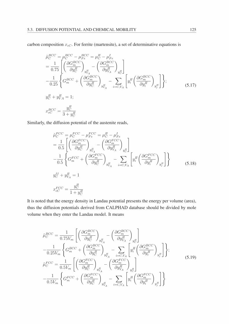
5.3. DIFFUSION POTENTIAL AND CHEMICAL MOBILITY 125
carbon composition xcC . For ferrite (martensite), a set of determinative equations is
μBCCC = μBCC
C − μBCCFe = μII
C − μIFe
=1
0.75
[(∂GBCC
m
∂yIIC
)yIIVA
−(∂GBCC
m
∂yIIVA
)yIIC
]
− 1
0.25
{GBCC
m +
(∂GBCC
m
∂yIIC
)yIIVA
−∑
i=C,VA
[yIIi
(∂GBCC
m
∂yIIi
)yIIj
]};
yIIC + yIIV A = 1;
xBCCcC =
yIIC3 + yIIC
(5.17)
Similarly, the diffusion potential of the austenite reads,
μFCCC = μFCC
C − μFCCFe = μII
C − μIFe
=1
0.5
[(∂GFCC
m
∂yIIC
)yIIVA
−(∂GFCC
m
∂yIIVA
)yIIC
]
− 1
0.5
{GFCC
m +
(∂GFCC
m
∂yIIC
)yIIVA
−∑
i=C,VA
[yIIi
(∂GFCC
m
∂yIIi
)yIIj
]}
yIIC + yIIVA= 1
xFCCcC =
yIIC1 + yIIC
(5.18)
It is noted that the energy density in Landau potential presents the energy per volume (area),
thus the diffusion potentials derived from CALPHAD database should be divided by mole
volume when they enter the Landau model. It means
μBCCC =
1
0.75Vm
[(∂GBCC
m
∂yIIC
)yIIVA
−(∂GBCC
m
∂yIIVA
)yIIC
]
− 1
0.25Vm
{GBCC
m +
(∂GBCC
m
∂yIIC
)yIIVA
−∑
i=C,VA
[yIIi
(∂GBCC
m
∂yIIi
)yIIj
]};
μFCCC =
1
0.5Vm
[(∂GFCC
m
∂yIIC
)yIIVA
−(∂GFCC
m
∂yIIVA
)yIIC
]
− 1
0.5Vm
{GFCC
m +
(∂GFCC
m
∂yIIC
)yIIVA
−∑
i=C,VA
[yIIi
(∂GFCC
m
∂yIIi
)yIIj
]}(5.19)
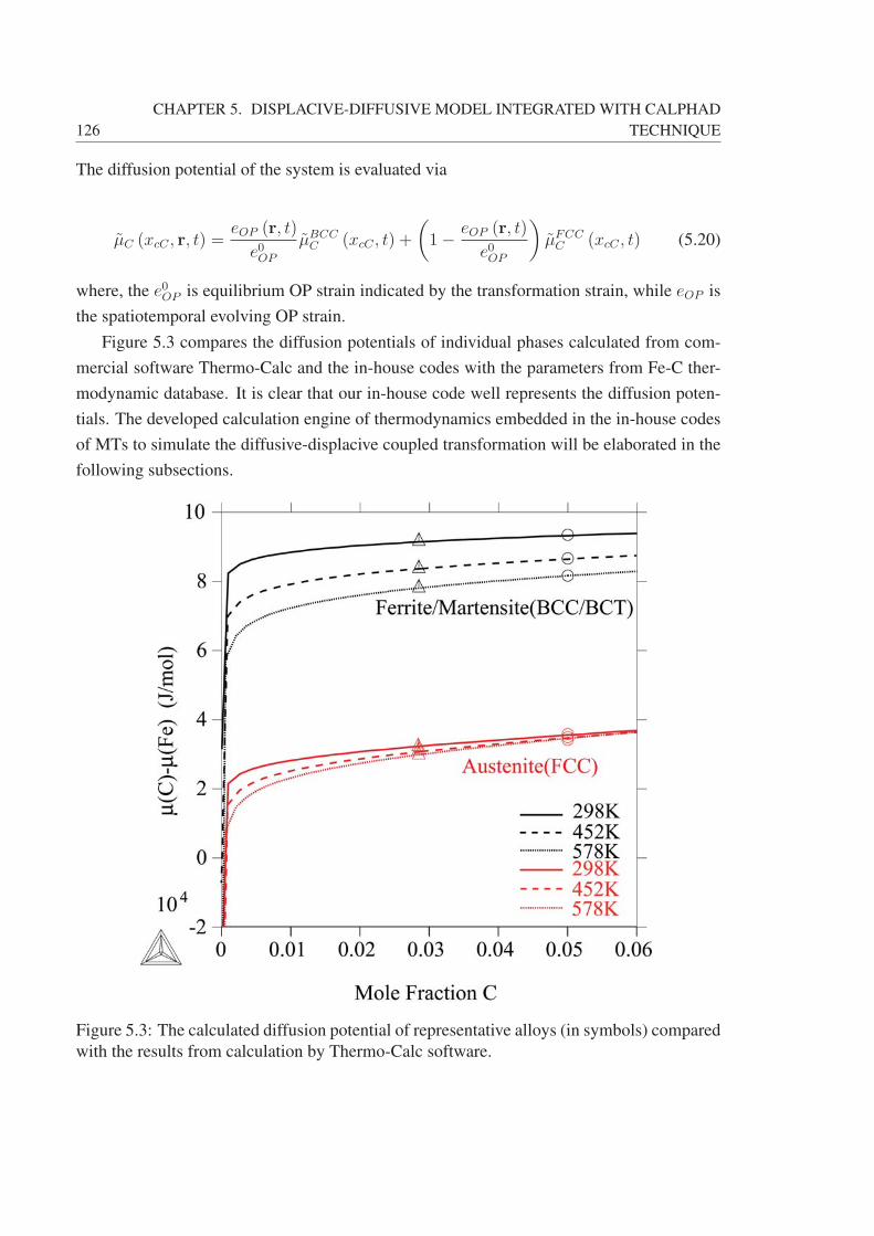
126
CHAPTER 5. DISPLACIVE-DIFFUSIVE MODEL INTEGRATED WITH CALPHAD
TECHNIQUE
The diffusion potential of the system is evaluated via
μC (xcC , r, t) =eOP (r, t)
e0OP
μBCCC (xcC , t) +
(1− eOP (r, t)
e0OP
)μFCCC (xcC , t) (5.20)
where, the e0OP is equilibrium OP strain indicated by the transformation strain, while eOP is
the spatiotemporal evolving OP strain.
Figure 5.3 compares the diffusion potentials of individual phases calculated from com-
mercial software Thermo-Calc and the in-house codes with the parameters from Fe-C ther-
modynamic database. It is clear that our in-house code well represents the diffusion poten-
tials. The developed calculation engine of thermodynamics embedded in the in-house codes
of MTs to simulate the diffusive-displacive coupled transformation will be elaborated in the
following subsections.
Figure 5.3: The calculated diffusion potential of representative alloys (in symbols) compared
with the results from calculation by Thermo-Calc software.

5.3. DIFFUSION POTENTIAL AND CHEMICAL MOBILITY 127
A (semi-)quantitative Landau modeling of displacive-diffusive coupled phase transfor-
mation also requires accurate chemical mobilities entering Cahn-Hilliard equation. The
chemical mobility is the functional of the atomic mobility. The latter can be directly ex-
tracted from multicomponent and multiphase diffusion kinetic database. In a natural way, it
bridges the computational diffusion kinetics and the Landau modeling of phase transforma-
tion. In computational diffusion kinetics, atomic mobility can be expressed as
M θi =
M θ0i
RTexp(− Qθ
i
RT) (5.21)
The M θ0i is a frequency factor, and the activation energy Qθ
i is written in CALPHAD fash-
ioned Redlish-Kister polynomial as
Qθi =∑p
xpQθi +∑p
∑q>p
xpxq
[ ∑r=0,1,2
rQp,qi (xp − xq)
r
](5.22)
for (sub)regular solution model, and
Qθi =∑j
∑m
yIj yIImQ
θ−j:mi +
∑j
∑k>j
∑m
yIj yIky
IIm
[ ∑r=0,1,2
rQθ−j,ki
(yIj − yIk
)r]
+∑j
∑m
∑n>m
yIj yIImy
IIn
[ ∑r=0,1,2
rQθ−m,ni
(yIIm − yIIn
)r] (5.23)
Table 5.1: The calculated chemical potentials and diffusion potentials (J/mol) of
BCC(martensite) and FCC(austenite) phases in two objective Fe-C alloys at different tem-
peratures
Cwt.% Potential Name Values
298.15K 452.95K 578.15K
0.59 μC.BCC 83238.62 70371.54 59450.16
0.59 μFe.BCC -8213.18 -13375.61 -18674.90
0.59 μBCC 91451.80 83747.14 78125.06
0.59 μC.FCC 29516.28 21336.58 14206.28
0.59 μFe.FCC -2836.82 -9332.61 -15678.98
0.59 μFCC 35353.10 30669.18 29885.26
1.07 μC.BCC 84959.09 72985.27 62786.36
1.07 μFe.BCC -8282.53 -13480.96 -18809.38
1.07 μBCC 93241.62 86466.23 81595.74
1.07 μC.FCC 32574.76 25159.59 18647.63
1.07 μFe.FCC -2961.29 -9487.78 -15858.99
1.07 μFCC 35536.05 34647.37 34506.62

128
CHAPTER 5. DISPLACIVE-DIFFUSIVE MODEL INTEGRATED WITH CALPHAD
TECHNIQUE
for the CEF sublattice model. The chemical mobilities M θkj in single phase are related to
atomic mobility M θi via the equations
M θkj =
1
Vm
∑l
(δjl − xcj) (δlk − xck) xclMθl
M θkj =
1
Vm
∑l
(δjl − ucj) (δlk − uck)uclMθl +
1
Vm
∑l /∈S
δjlyIIV AuclM
θl
(5.24)
where δjl and δlk are the Kronecker delta. In binary Fe-C system, M θCC is served as the
exclusive independent variables. Therefore,
MFCCCC =
1
Vm
(x2cFexcCM
FCCC + x2
cCxcFeMFCCFe
) ≈ 1
Vm
x2cFexcCM
FCCC
MBCCCC =
1
Vm
(x2cFexcCM
BCCC + x2
cCxcFeMBCCFe
) ≈ 1
Vm
x2cFexcCM
BCCC
(5.25)
In a structural and compositional non-uniform system, the same relation between Mkj and
Mi should hold for entire system, while the atomic mobility is spatiotemporally dependent
and coupled with the OP strain in displacive transformation via
Ml = MBCCl +MFCC
l − (MBCCl
)eOP /e0OP(MFCC
l
)(1−eOP /e0OP ) (5.26)
Thus, the approximated chemical mobility in Landau modeling is expressed as
MCC =1
Vm
(x2cFexcCMC + x2
cCxcFeMFe)
≈ 1
Vm
x2cFexcCMC =
1
Vm
x2cFexcC
[MBCC
C +MFCCC − (MBCC
C
)eOP /e0OP(MFCC
C
)(1−eOP /e0OP )]
(5.27)
5.4 Coupled Model and Semi-quantification
In this section, the Landau model in chapter 3 is further developed by adding the energy
contributions of chemistry. The coupled model is designed to simulate the microstructure
of steel and its evolution in polycrystals. In this displacive-diffusive coupled model, the
symmetry adapted deviatoric strain e2, spatiotemporal distribution of the carbon composition
xcC and grain orientations ηi are selected as field variables. With the field variables, one can
5.4. COUPLED MODEL AND SEMI-QUANTIFICATION 129
distinguish the domains of martensite variants and austenite by a combination of strain and
composition. The total free energy of the system is expressed as
F =
∫d�r(fel + fch + fgrain + fcpl + fgradc + fgrade) (5.28)
and is composed of the non-linear elastic free energy−fel, the chemical free energy−fch,
the grain boundary energy fgrain, the coupling energy contributions −fcpl and the chemi-
cal (fgradc) and elastic (fgrade) gradient energy [BA06, BA07]. According to the nonlinear
Landau model in chapter 3, the square-to-rectangular MT is described by a 2-4-6 Landau
polynomial with the primary OP of deviatoric strain e2, i.e.
fel = (c11 + c12)[e1 − κ1cxc − κ12e
22
]2+ 2c44e
23 + (c11 − c12) e
22 +Be42 + Ce62 (5.29)
here, the influences of OP strain and composition on the bulk dilatation are taken into con-
sideration that become significant when the directions of habit planes deviate from those of
twin planes.
In our model, the diffusion potential detailed in the section 5.3 instead ofδfchδxcC
enters
the Cahn-Hilliard equation to solve the diffusion of carbon, thus the expression of chemical
energy in CALPHAD is not necessary explicitly given here. The grain boundary energy has
the same expression as that in chapters 3 and 4, which is no longer repeated here. However,
for a semi-quantitative simulation, an appropriate normalization factor of m = 0.01 is mul-
tiplied in front of fgrain to correctly describe the small value of the grain boundary energy
density around 1.0J/m2 [RSM+13].
Besides the above energy contributions, various coupling effects are included in our cou-
pled model. Although the continuous grain boundary model in chapter 3 successfully de-
scribed the grain boundary nucleation assisted with gradient of OP strain in polycrystals,
the grain boundary relaxation of the localized strain is not included. In this chapter, an
additional coupling term between shape function of grain boundaries and strain gradienta12(∇e2)
2Q∑i
(∇ηi)2
is incorporated in Landau free energy. (Figure 5.4 illustrates the simu-
lated morphology of polycrystals by using the shape function of grain boundariesQ∑i
(∇ηi)2.)
The starting point of incorporating this dual-gradient term is based on the experimental dis-
covery that the coupling of strain gradient and grain orientation does effect on the mechanical
properties by our colleagues. To ensure the formal integrity of the coupling effect, a con-
ventional coupling between strain itself and shape function of grain orientation is also taken,
namely,a02e22
Q∑i
(∇ηi)2, which has ability to account for suppression effect of grain bound-

130
CHAPTER 5. DISPLACIVE-DIFFUSIVE MODEL INTEGRATED WITH CALPHAD
TECHNIQUE
Figure 5.4: The morphology of grain boundary represented by the shape functionsQ∑i
(∇ηi)2
ary on MT in some nano-sized polycrystals. The solute drag effect at the grain boundary is
simplified as κcgxcCmfgrain, and the coupling between elastic distortions and composition
is introduced as κcee22x
2cC with a 2-2 fourth order power function appropriate for all the crys-
tallographic symmetry. Therefore, a complete nonlinear Landau energy for the displacive-
diffusive coupled phase transformation can be written in
F =
∫dr
⎧⎪⎪⎪⎪⎪⎪⎨⎪⎪⎪⎪⎪⎪⎩
(c11 + c12)[e1 − κ1cxc − κ12e
22
]2+ 2c44e
23 + (c11 − c12) e
22 +Be42
+Be62 + fch +mfgrain +ge2(∇e2)
2 +gc2(∇xcC)
2 +a02e22
Q∑i
(∇ηi)2
+a12(∇e2)
2Q∑i
(∇ηi)2 + κcgxcCmfgrain + κcee
22x
2cC
⎫⎪⎪⎪⎪⎪⎪⎬⎪⎪⎪⎪⎪⎪⎭
(5.30)
With the function of Landau free energy, the semi-quantification of Landau free energy
for MT in steel was carried out. From thermodynamics of MT, the martensitic nucleation in
steel is no longer attributed to the acoustic lattice softening of the phonons with a small wave
vector, which was evidenced by the negative temperature dependence of elastic constants.
The temperature dependence of the bulk and shear moduli of BCC iron was measured by
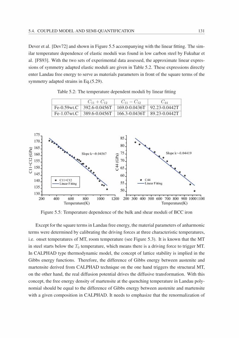
5.4. COUPLED MODEL AND SEMI-QUANTIFICATION 131
Dever et al. [Dev72] and shown in Figure 5.5 accompanying with the linear fitting. The sim-
ilar temperature dependence of elastic moduli was found in low carbon steel by Fukuhar et
al. [FS93]. With the two sets of experimental data assessed, the approximate linear expres-
sions of symmetry adapted elastic moduli are given in Table 5.2. These expressions directly
enter Landau free energy to serve as materials parameters in front of the square terms of the
symmetry adapted strains in Eq.(5.29).
Table 5.2: The temperature dependent moduli by linear fitting
C11 + C12 C11 − C12 C44
Fe-0.59wt.C 392.6-0.0456T 169.0-0.0436T 92.23-0.0442T
Fe-1.07wt.C 389.6-0.0456T 166.3-0.0436T 89.23-0.0442T
Figure 5.5: Temperature dependence of the bulk and shear moduli of BCC iron
Except for the square terms in Landau free energy, the material parameters of anharmonic
terms were determined by calibrating the driving forces at three characteristic temperatures,
i.e. onset temperatures of MT, room temperature (see Figure 5.3). It is known that the MT
in steel starts below the T0 temperature, which means there is a driving force to trigger MT.
In CALPHAD type thermodynamic model, the concept of lattice stability is implied in the
Gibbs energy functions. Therefore, the difference of Gibbs energy between austenite and
martensite derived from CALPHAD technique on the one hand triggers the structural MT,
on the other hand, the real diffusion potential drives the diffusive transformation. With this
concept, the free energy density of martensite at the quenching temperature in Landau poly-
nomial should be equal to the difference of Gibbs energy between austenite and martensite
with a given composition in CALPHAD. It needs to emphasize that the renormalization of

132
CHAPTER 5. DISPLACIVE-DIFFUSIVE MODEL INTEGRATED WITH CALPHAD
TECHNIQUE
the Landau potential for MT at each time step is still open, although the seamless integration
with CALPHAD technique in our model ensures the real time diffusion potential in each
grid in simulation box and at each time step can be calculated. To semi-quantitatively de-
scribe the driving force of MT, the material coefficients of anharmonic terms in Eq.(5.30)
were adjusted to determine the Landau free energy. The values of energy wells on Landau
energy surface were calibrated against the thermodynamic driving forces at Ms and room
temperatures, and the transformation strains indicated by energy wells were adjusted in ac-
cordance with experiments data. Figure 5.6 shows the normalized Landau free energy of Fe-
0.59wt% C and Fe-1.07wt% C with a normalized energy density factor of 2.52× 10¹¹J/m2
and 2.06× 10¹¹J/m2, respectively, at room, Ms, and partitioning temperatures.
Figure 5.6: Normalized Landau free energy at room, Ms, and partitioning temperatures,
which are calibrated with thermodynamic database. The upper panel is the energies of Fe-
0.59wt% C alloy, and the bottom panel is for Fe-1.07wt% C
The numerical procedures for simulating MT have been detailed in section 3.3 by solv-
ing the general equation of motion Eq.(3.8). For displacive-diffusive coupled transformation,
the Cahn-Hilliard equation is used to monitor the spatiotemporal redistribution of carbon el-
ement with the chemical mobility associated with the atomic mobility from kinetic database
of CALPHAD method. The chemical mobility in Eq.(5.31) varies with coordinates and time,
5.5. MICROSTRUCTURE EVOLUTION 133
rather than a constant in most of conventional phase field modeling.
∂xcC(�r, t)
∂t= ∇MC(�r, t)∇
(δF (�r, t)
δxcC(�r, t)− gc∇2xcC(�r, t)
)(5.31)
The numerical treatment of explicit finite difference in time and semi-implicit spectral scheme
in space is widely accepted in computer simulation of Cahn-Hilliard equation. To overcome
the time-step constraint, a term 0.5gck4xcC (k, t) was added to both sides of equation in the
conventional first-order semi-implicit Fourier spectral scheme [ZCST99], which leads to
NL = F
(δF (�r, t)
δxcC(�r, t)
)(1 + 0.5Δtgck
4)x(n+1)cC (k, t) =
(1 + 0.5Δtgck
4)x(n)cC (k, t)
+ ΔtikF{MC(�r, t)F
−1(ik[NL+ gck
2x(n)cC (k, t)
])} (5.32)
where F and F−1 denote Fourier and inverse Fourier transformations, respectively.
5.5 Microstructure Evolution
5.5.1 Grain Boundary Nucleation and Growth
To examine the martensitic nucleation and growth assisted with grain boundary, a 2D
bicrystal benchmark containing two grains of θ = 0 and π/6 was firstly employed, as is
shown in Figure 5.7a. The two grains are separated by a flat grain boundary with the nor-
malization factor of m = 0.01 for grain boundary energy. Although the grain boundary
nucleation can be realized without the coupling term in chapter 4, the coupling gradients
representing the strain relaxation at grain boundary was added to facilitate the nucleation of
martensite. The dual-gradient coupling coefficient was set at a1=0.7, while the direct cou-
pling was set a0=0, which avoids the inhibition of grain boundary nucleation. The value of
dilatation coupling coefficient κ12 between e1 and e2 was set to 1.25. The random fluctu-
ations of displacement following the Gaussian distribution were incorporated at the initial
stage. Figure 5.7 illustrates the temporal evolution of martensite variants as the results of
isothermal simulation after quenched the Fe-0.59% C alloy to the room temperature. At
the room temperature lower than the Ms, the nucleation of martensites can occur due to the
lowered stability of the austenite with respect to the martensite. It is clear that two types
of martensite variants, represented in red and blue, promptly nucleate at the grain boundary
preceding those in bulk counterpart. The phenomenon originates from the reduced nucle-
ation barrier for the formation of martensites at grain boundary due to the coupling between
the grain boundary and the non-local strain gradient, which accounts for the extra relaxation
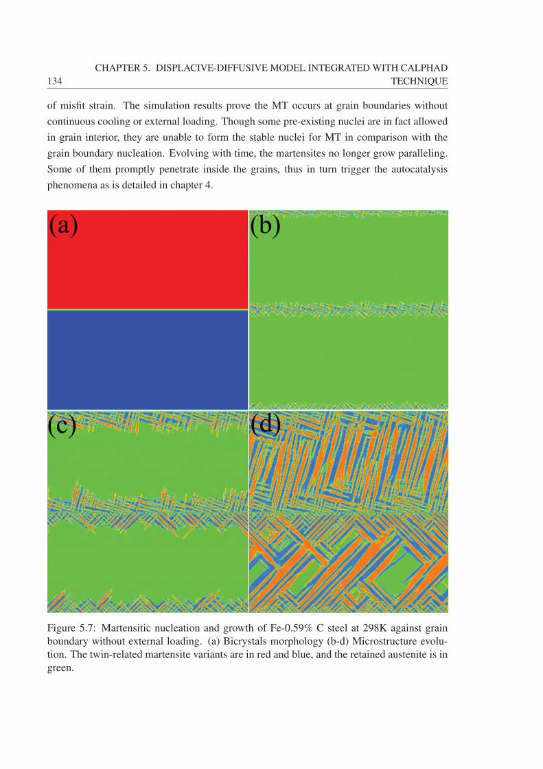
134
CHAPTER 5. DISPLACIVE-DIFFUSIVE MODEL INTEGRATED WITH CALPHAD
TECHNIQUE
of misfit strain. The simulation results prove the MT occurs at grain boundaries without
continuous cooling or external loading. Though some pre-existing nuclei are in fact allowed
in grain interior, they are unable to form the stable nuclei for MT in comparison with the
grain boundary nucleation. Evolving with time, the martensites no longer grow paralleling.
Some of them promptly penetrate inside the grains, thus in turn trigger the autocatalysis
phenomena as is detailed in chapter 4.
Figure 5.7: Martensitic nucleation and growth of Fe-0.59% C steel at 298K against grain
boundary without external loading. (a) Bicrystals morphology (b-d) Microstructure evolu-
tion. The twin-related martensite variants are in red and blue, and the retained austenite is in
green.
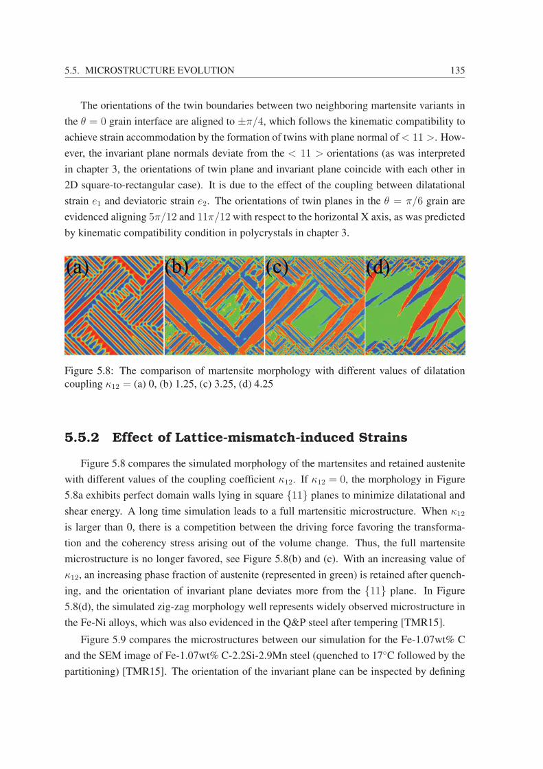
5.5. MICROSTRUCTURE EVOLUTION 135
The orientations of the twin boundaries between two neighboring martensite variants in
the θ = 0 grain interface are aligned to ±π/4, which follows the kinematic compatibility to
achieve strain accommodation by the formation of twins with plane normal of < 11 >. How-
ever, the invariant plane normals deviate from the < 11 > orientations (as was interpreted
in chapter 3, the orientations of twin plane and invariant plane coincide with each other in
2D square-to-rectangular case). It is due to the effect of the coupling between dilatational
strain e1 and deviatoric strain e2. The orientations of twin planes in the θ = π/6 grain are
evidenced aligning 5π/12 and 11π/12 with respect to the horizontal X axis, as was predicted
by kinematic compatibility condition in polycrystals in chapter 3.
Figure 5.8: The comparison of martensite morphology with different values of dilatation
coupling κ12 = (a) 0, (b) 1.25, (c) 3.25, (d) 4.25
5.5.2 Effect of Lattice-mismatch-induced Strains
Figure 5.8 compares the simulated morphology of the martensites and retained austenite
with different values of the coupling coefficient κ12. If κ12 = 0, the morphology in Figure
5.8a exhibits perfect domain walls lying in square {11} planes to minimize dilatational and
shear energy. A long time simulation leads to a full martensitic microstructure. When κ12
is larger than 0, there is a competition between the driving force favoring the transforma-
tion and the coherency stress arising out of the volume change. Thus, the full martensite
microstructure is no longer favored, see Figure 5.8(b) and (c). With an increasing value of
κ12, an increasing phase fraction of austenite (represented in green) is retained after quench-
ing, and the orientation of invariant plane deviates more from the {11} plane. In Figure
5.8(d), the simulated zig-zag morphology well represents widely observed microstructure in
the Fe-Ni alloys, which was also evidenced in the Q&P steel after tempering [TMR15].
Figure 5.9 compares the microstructures between our simulation for the Fe-1.07wt% C
and the SEM image of Fe-1.07wt% C-2.2Si-2.9Mn steel (quenched to 17◦C followed by the
partitioning) [TMR15]. The orientation of the invariant plane can be inspected by defining
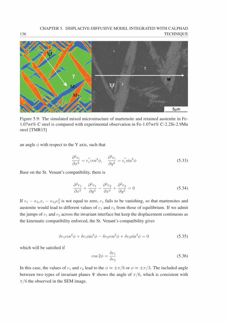
136
CHAPTER 5. DISPLACIVE-DIFFUSIVE MODEL INTEGRATED WITH CALPHAD
TECHNIQUE
Figure 5.9: The simulated mixed microstructure of martensite and retained austenite in Fe-
1.07wt% C steel is compared with experimental observation in Fe-1.07wt% C-2.2Si-2.9Mn
steel [TMR15]
an angle φ with respect to the Y axis, such that
∂2ei∂x2
= e′′i cos
2φ,∂2ei∂y2
= e′′i sin
2φ (5.33)
Base on the St. Venant’s compatibility, there is
∂2e1∂x2
+∂2e1∂y2
− ∂2e2∂x2
+∂2e2∂y2
= 0 (5.34)
If e1 − κ1cxc − κ12e22 is not equal to zero, e1 fails to be vanishing, so that martensites and
austenite would lead to different values of e1 and e2 from those of equilibrium. If we admit
the jumps of e1 and e2 across the invariant interface but keep the displacement continuous as
the kinematic compatibility enforced, the St. Venant’s compatibility gives
δe1cos2φ+ δe1sin
2φ− δe2cos2φ+ δe2sin
2φ = 0 (5.35)
which will be satisfied if
cos 2φ =δe1δe2
(5.36)
In this case, the values of e1 and e2 lead to the φ ≈ ±π/6 or φ ≈ ±π/3. The included angle
between two types of invariant planes Ψ shows the angle of π/6, which is consistent with
π/6 the observed in the SEM image.

5.5. MICROSTRUCTURE EVOLUTION 137
5.5.3 Carbon Redistribution in As-quenched Microstruc-ture
The short-range diffusion of carbon from martensite to austenite in Fe-0.59wt% C is
clearly observed in Fig. 5.10(b); especially, the carbon element is segregated at the marten-
site / austenite (α′/γ) interfaces colored in yellow and orange. Simulation confirms that
diffusion potential at the room temperature provides chemical driving force to diffusion.
However, the atomic diffusion mobility of carbon in martensite is about seven orders of
magnitudes greater than that in austenite. The synergy of diffusion potential and chemical
mobility led to a strong redistribution of carbon characterized in its segregation at α′/γ inter-
faces. Therefore, it has demonstrated that the partitioning or compositional redistribution of
carbon in Q&P steels is the inherent behavior of the diffusion, and is nothing special in com-
parison with the ordinary diffusional transformations, which are all governed by diffusion
potential and chemical mobility. The only peculiarity is the effect of short-range diffusion
or relaxation of carbon is smeared out in the displacive MT, which was hardly to be detected
until the maturity of 3DAP technique.
Figure 5.10: (a) The as-quenched mixed microstructure of martensite and austenite and (b)
carbon distribution in Fe-0.59wt% C alloy at 298K
Recently, Toji et al. [TMH+14] adopted 3DAP to study the carbon partitioning in Q&P
steel with the composition Fe-0.59wt%C-2.0Si-2.9Mn, and presented a direct atomic scale
evidence of carbon partitioning from martensite to austenite without the presence of bainite
transformation. In their 3DAP observation, the carbon concentration fluctuated in the range
between 1.5 at.% and 4.5 at.% in the as-quenched sample, giving the average carbon concen-
tration of 2.77 at.%, in good agreement with the bulk carbon content of the steel (2.7 at.%).
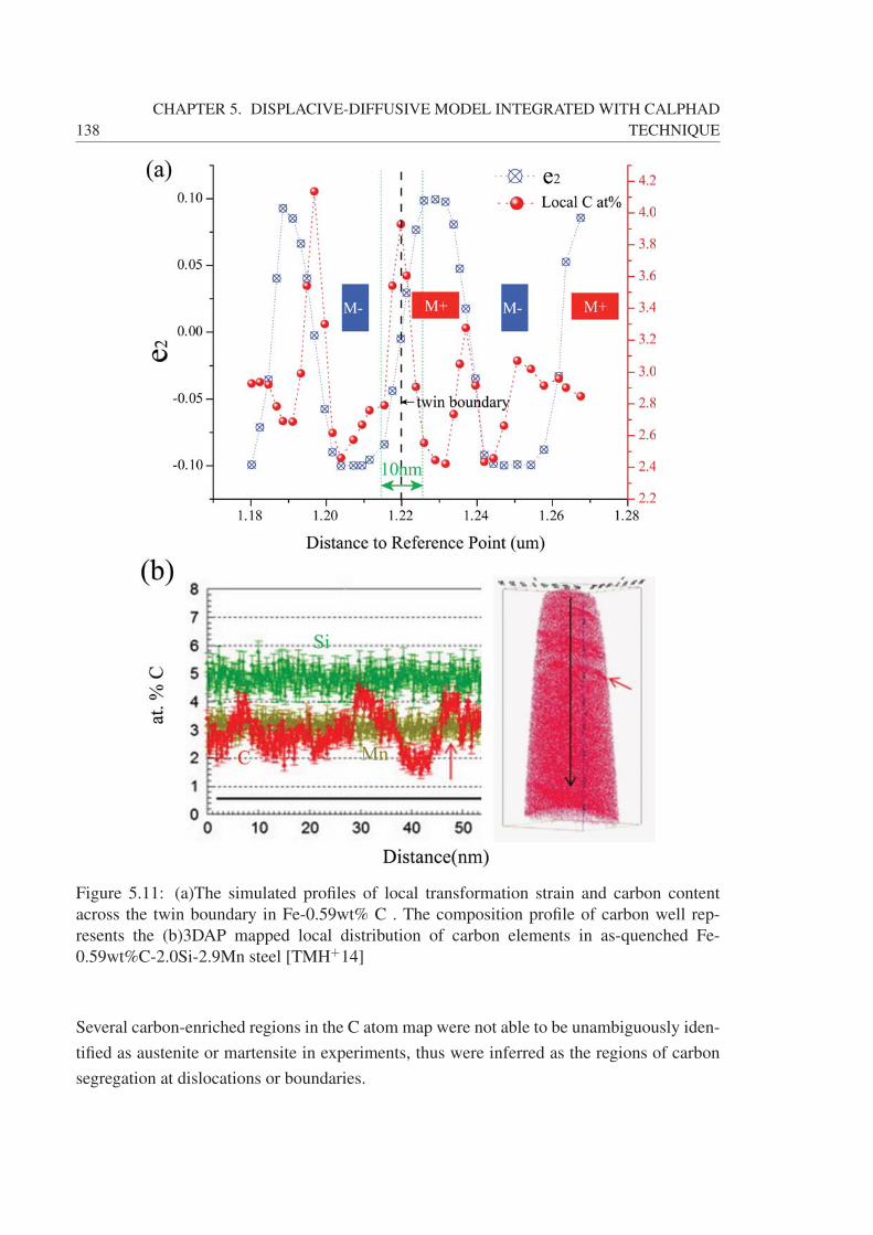
138
CHAPTER 5. DISPLACIVE-DIFFUSIVE MODEL INTEGRATED WITH CALPHAD
TECHNIQUE
Figure 5.11: (a)The simulated profiles of local transformation strain and carbon content
across the twin boundary in Fe-0.59wt% C . The composition profile of carbon well rep-
resents the (b)3DAP mapped local distribution of carbon elements in as-quenched Fe-
0.59wt%C-2.0Si-2.9Mn steel [TMH+14]
Several carbon-enriched regions in the C atom map were not able to be unambiguously iden-
tified as austenite or martensite in experiments, thus were inferred as the regions of carbon
segregation at dislocations or boundaries.
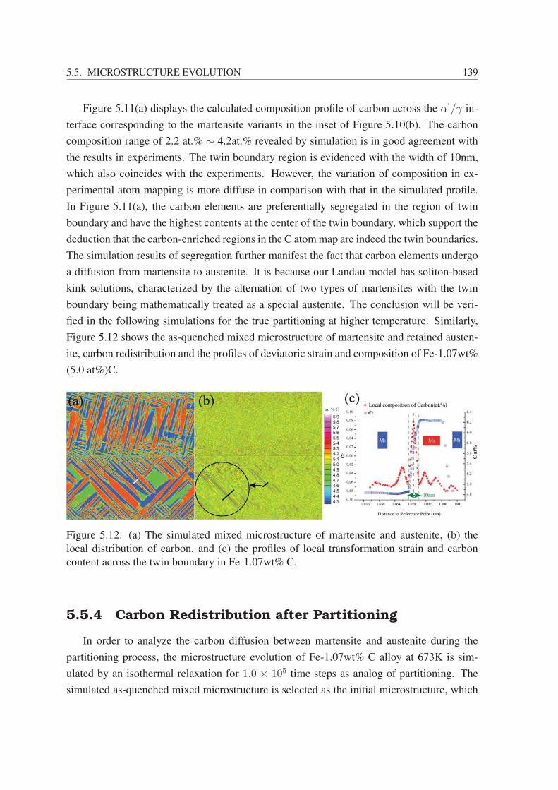
5.5. MICROSTRUCTURE EVOLUTION 139
Figure 5.11(a) displays the calculated composition profile of carbon across the α′/γ in-
terface corresponding to the martensite variants in the inset of Figure 5.10(b). The carbon
composition range of 2.2 at.% ∼ 4.2at.% revealed by simulation is in good agreement with
the results in experiments. The twin boundary region is evidenced with the width of 10nm,
which also coincides with the experiments. However, the variation of composition in ex-
perimental atom mapping is more diffuse in comparison with that in the simulated profile.
In Figure 5.11(a), the carbon elements are preferentially segregated in the region of twin
boundary and have the highest contents at the center of the twin boundary, which support the
deduction that the carbon-enriched regions in the C atom map are indeed the twin boundaries.
The simulation results of segregation further manifest the fact that carbon elements undergo
a diffusion from martensite to austenite. It is because our Landau model has soliton-based
kink solutions, characterized by the alternation of two types of martensites with the twin
boundary being mathematically treated as a special austenite. The conclusion will be veri-
fied in the following simulations for the true partitioning at higher temperature. Similarly,
Figure 5.12 shows the as-quenched mixed microstructure of martensite and retained austen-
ite, carbon redistribution and the profiles of deviatoric strain and composition of Fe-1.07wt%
(5.0 at%)C.
Figure 5.12: (a) The simulated mixed microstructure of martensite and austenite, (b) the
local distribution of carbon, and (c) the profiles of local transformation strain and carbon
content across the twin boundary in Fe-1.07wt% C.
5.5.4 Carbon Redistribution after Partitioning
In order to analyze the carbon diffusion between martensite and austenite during the
partitioning process, the microstructure evolution of Fe-1.07wt% C alloy at 673K is sim-
ulated by an isothermal relaxation for 1.0 × 10⁵ time steps as analog of partitioning. The
simulated as-quenched mixed microstructure is selected as the initial microstructure, which
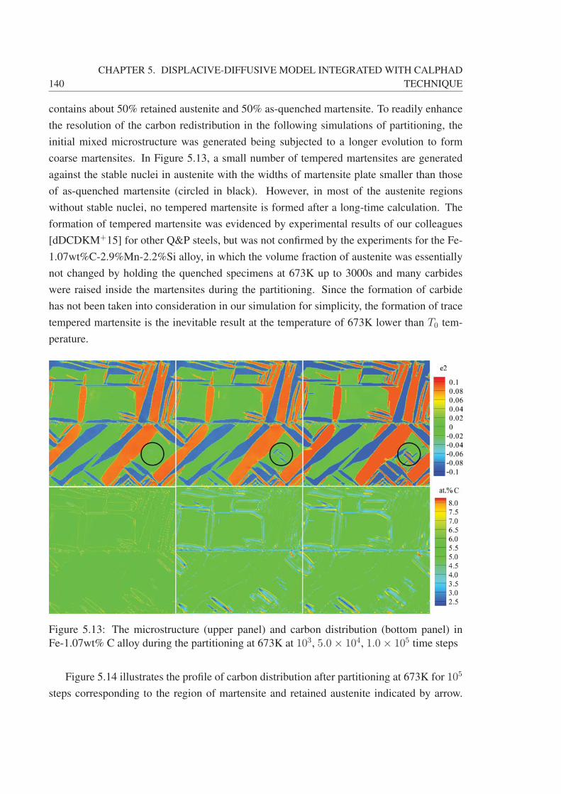
140
CHAPTER 5. DISPLACIVE-DIFFUSIVE MODEL INTEGRATED WITH CALPHAD
TECHNIQUE
contains about 50% retained austenite and 50% as-quenched martensite. To readily enhance
the resolution of the carbon redistribution in the following simulations of partitioning, the
initial mixed microstructure was generated being subjected to a longer evolution to form
coarse martensites. In Figure 5.13, a small number of tempered martensites are generated
against the stable nuclei in austenite with the widths of martensite plate smaller than those
of as-quenched martensite (circled in black). However, in most of the austenite regions
without stable nuclei, no tempered martensite is formed after a long-time calculation. The
formation of tempered martensite was evidenced by experimental results of our colleagues
[dDCDKM+15] for other Q&P steels, but was not confirmed by the experiments for the Fe-
1.07wt%C-2.9%Mn-2.2%Si alloy, in which the volume fraction of austenite was essentially
not changed by holding the quenched specimens at 673K up to 3000s and many carbides
were raised inside the martensites during the partitioning. Since the formation of carbide
has not been taken into consideration in our simulation for simplicity, the formation of trace
tempered martensite is the inevitable result at the temperature of 673K lower than T0 tem-
perature.
Figure 5.13: The microstructure (upper panel) and carbon distribution (bottom panel) in
Fe-1.07wt% C alloy during the partitioning at 673K at 103, 5.0× 10⁴, 1.0× 10⁵ time steps
Figure 5.14 illustrates the profile of carbon distribution after partitioning at 673K for 105
steps corresponding to the region of martensite and retained austenite indicated by arrow.
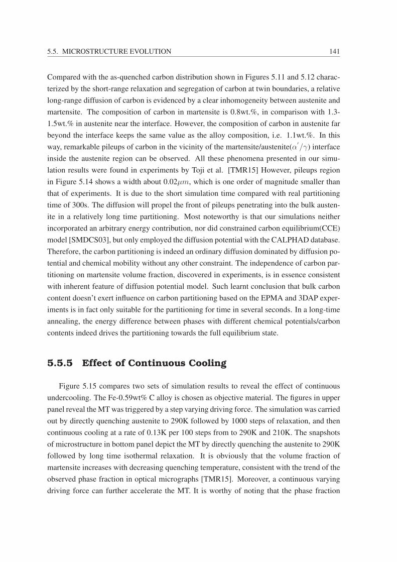
5.5. MICROSTRUCTURE EVOLUTION 141
Compared with the as-quenched carbon distribution shown in Figures 5.11 and 5.12 charac-
terized by the short-range relaxation and segregation of carbon at twin boundaries, a relative
long-range diffusion of carbon is evidenced by a clear inhomogeneity between austenite and
martensite. The composition of carbon in martensite is 0.8wt.%, in comparison with 1.3-
1.5wt.% in austenite near the interface. However, the composition of carbon in austenite far
beyond the interface keeps the same value as the alloy composition, i.e. 1.1wt.%. In this
way, remarkable pileups of carbon in the vicinity of the martensite/austenite(α′/γ) interface
inside the austenite region can be observed. All these phenomena presented in our simu-
lation results were found in experiments by Toji et al. [TMR15] However, pileups region
in Figure 5.14 shows a width about 0.02μm, which is one order of magnitude smaller than
that of experiments. It is due to the short simulation time compared with real partitioning
time of 300s. The diffusion will propel the front of pileups penetrating into the bulk austen-
ite in a relatively long time partitioning. Most noteworthy is that our simulations neither
incorporated an arbitrary energy contribution, nor did constrained carbon equilibrium(CCE)
model [SMDCS03], but only employed the diffusion potential with the CALPHAD database.
Therefore, the carbon partitioning is indeed an ordinary diffusion dominated by diffusion po-
tential and chemical mobility without any other constraint. The independence of carbon par-
titioning on martensite volume fraction, discovered in experiments, is in essence consistent
with inherent feature of diffusion potential model. Such learnt conclusion that bulk carbon
content doesn’t exert influence on carbon partitioning based on the EPMA and 3DAP exper-
iments is in fact only suitable for the partitioning for time in several seconds. In a long-time
annealing, the energy difference between phases with different chemical potentials/carbon
contents indeed drives the partitioning towards the full equilibrium state.
5.5.5 Effect of Continuous Cooling
Figure 5.15 compares two sets of simulation results to reveal the effect of continuous
undercooling. The Fe-0.59wt% C alloy is chosen as objective material. The figures in upper
panel reveal the MT was triggered by a step varying driving force. The simulation was carried
out by directly quenching austenite to 290K followed by 1000 steps of relaxation, and then
continuous cooling at a rate of 0.13K per 100 steps from to 290K and 210K. The snapshots
of microstructure in bottom panel depict the MT by directly quenching the austenite to 290K
followed by long time isothermal relaxation. It is obviously that the volume fraction of
martensite increases with decreasing quenching temperature, consistent with the trend of the
observed phase fraction in optical micrographs [TMR15]. Moreover, a continuous varying
driving force can further accelerate the MT. It is worthy of noting that the phase fraction
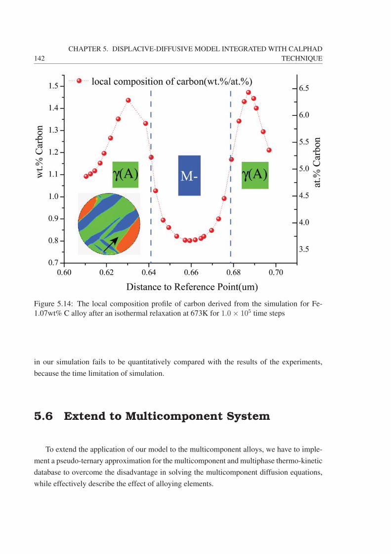
142
CHAPTER 5. DISPLACIVE-DIFFUSIVE MODEL INTEGRATED WITH CALPHAD
TECHNIQUE
Figure 5.14: The local composition profile of carbon derived from the simulation for Fe-
1.07wt% C alloy after an isothermal relaxation at 673K for 1.0× 10⁵ time steps
in our simulation fails to be quantitatively compared with the results of the experiments,
because the time limitation of simulation.
5.6 Extend to Multicomponent System
To extend the application of our model to the multicomponent alloys, we have to imple-
ment a pseudo-ternary approximation for the multicomponent and multiphase thermo-kinetic
database to overcome the disadvantage in solving the multicomponent diffusion equations,
while effectively describe the effect of alloying elements.
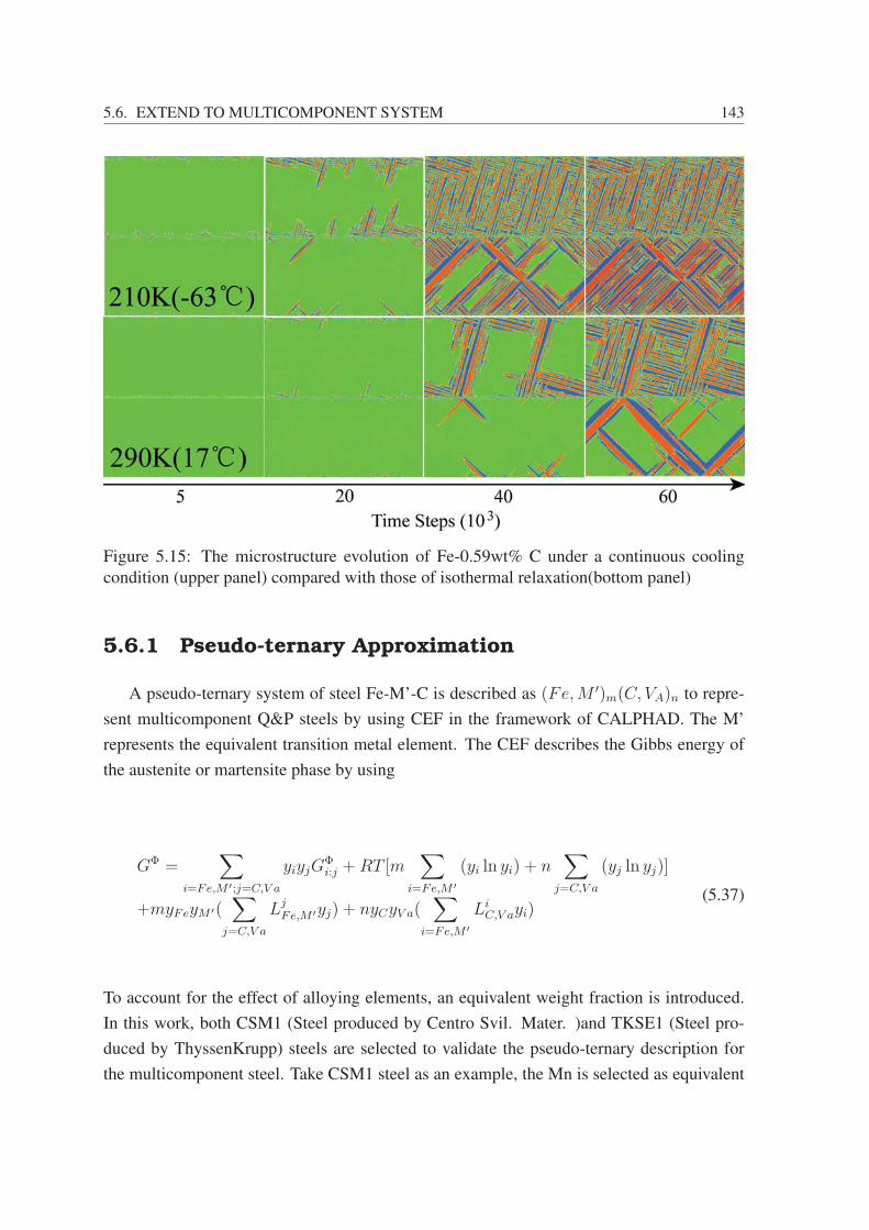
5.6. EXTEND TO MULTICOMPONENT SYSTEM 143
Figure 5.15: The microstructure evolution of Fe-0.59wt% C under a continuous cooling
condition (upper panel) compared with those of isothermal relaxation(bottom panel)
5.6.1 Pseudo-ternary Approximation
A pseudo-ternary system of steel Fe-M’-C is described as (Fe,M ′)m(C, VA)n to repre-
sent multicomponent Q&P steels by using CEF in the framework of CALPHAD. The M’
represents the equivalent transition metal element. The CEF describes the Gibbs energy of
the austenite or martensite phase by using
GΦ =∑
i=Fe,M ′;j=C,V a
yiyjGΦi:j +RT [m
∑i=Fe,M ′
(yi ln yi) + n∑
j=C,V a
(yj ln yj)]
+myFeyM ′(∑
j=C,V a
LjFe,M ′yj) + nyCyV a(
∑i=Fe,M ′
LiC,V ayi)
(5.37)
To account for the effect of alloying elements, an equivalent weight fraction is introduced.
In this work, both CSM1 (Steel produced by Centro Svil. Mater. )and TKSE1 (Steel pro-
duced by ThyssenKrupp) steels are selected to validate the pseudo-ternary description for
the multicomponent steel. Take CSM1 steel as an example, the Mn is selected as equivalent

144
CHAPTER 5. DISPLACIVE-DIFFUSIVE MODEL INTEGRATED WITH CALPHAD
TECHNIQUE
element, such thatwMn′ = λMnwMn + λSiwSi,
xMn′ = λMnxMn + λSixSiMSi
A
MMnA
;
λMn = 1,λSi = −0.4
(5.38)
where λ is equivalent coefficient, w and x are wright and mole fractions.
While for TKSE1 steel, the Si element equivalent is adopted because Si is a major alloying
element,
wSi′ = λSiwSi + λMnwMn + λCrwCr + λAlwAl;λAl = λSi = 1,λCr = 0.1,λMn = −0.5
xSi′ = λSixSi + λMnxMnMMn
A
MSiA
+ λCrxCrMCr
A
MSiA
+ λAlxAlMAl
A
MSiA
(5.39)
With the definition of the equivalent element, the thermodynamic database should be re-
assessed by calibrating the phase diagram and Ms temperature. The upgrading of thermody-
namic model for martensite is following the strategy of Ghosh and Olson [GO94a, GO94b].
The Gibbs energy of martensite can be derived from the critical condition for fcc → bcc
transformation via:
GM = GA + Vm(Δgch + gel +2σ
nd−Wfr) = GF + Vm(gel +
2σ
nd−Wfr) (5.40)
where GM and GA are Gibbs energy of martensite and austenite. Δgch is the chemical Gibbs
energy difference between ferrite and austenite, gel is strain energy per unit volume, σ is
interface energy, n is the number of close-packed planes comprising the nucleus thickness,
d is the spacing between close-packed planes, and W is interface frictional work. W can be
described as the function of shear modulus χ, i.e.
W = Kχχ(xj, T )
χ(xj, T ) = 1010 ×(9.2468 +
∑xj(
dχ
dxj
)
)[1− 7.9921× 10⁻⁷T 2 + 3.317× 10⁻¹⁰T 3
](5.41)
where the constant 9.2468 is the reference shear modulus of pure iron in austenitic state, and
the summation term is shear modulus contribution that changes austenite to martensite.
By adding the contributions from elastic strain, interfaces and friction into Gibbs enenrgy,
and then fitting both thermodynamic and phase transformation data from experiments and
literature, the parameters in our thermodynamic model for martensite are optimized.

5.6. EXTEND TO MULTICOMPONENT SYSTEM 145
Figure 5.16 illustrates the calculated composition dependence of the Ms temperature in
comparison with assessed Ms temperature of TKSE1 steel from experiments.
Figure 5.16: The calculated metastable isopleth of M/A transus
The calculated isopleths by using the assessed thermodynamic database of pseudo-ternary
Fe-M’-C are shown in Figure 5.17. The temperatures of autenite-ferrite transition have been
adopted as the fitting property. The results in Figure 5.17 represent the transition temper-
atures in good comparison with the results calculated with full multicomponent thermo-
dynamic database by using Thermo-Calc software. In Fig.5.17(b), the calculated equilib-
rium transition temperature is also compared with experimental Ac3 temperature in non-
equilibrium condition. The developed thermodynamic database is going to be updated as the
accumulating experimental data such as the phase fraction at different processing.
With the updated thermodynamic description, the Landau modeling for a multicompo-
nent system can be straightforwardly carried out by the method in this chapter with a full
Landau potential of
F =
∫dr{c11 + 2c12
3[e1 − κ1cxcC − κ1MxcM ′ − κ12
(e22 + e23
)]2 + 2c44
4−6∑i=4
e2i
+c11 − c12
2
(e22 + e23
)+
1
6√6(c111 − 3c112 + 2c123)e3
(e23 − 3e22
)+ C
(e22 + e23
)2+Gch + κce
(e22 + e23
)(x2
c + x2M) +
ge2[(∇e2)
2 + (∇e3)2] +
gc2[(∇xc)
2 + (∇xM)2]}(5.42)
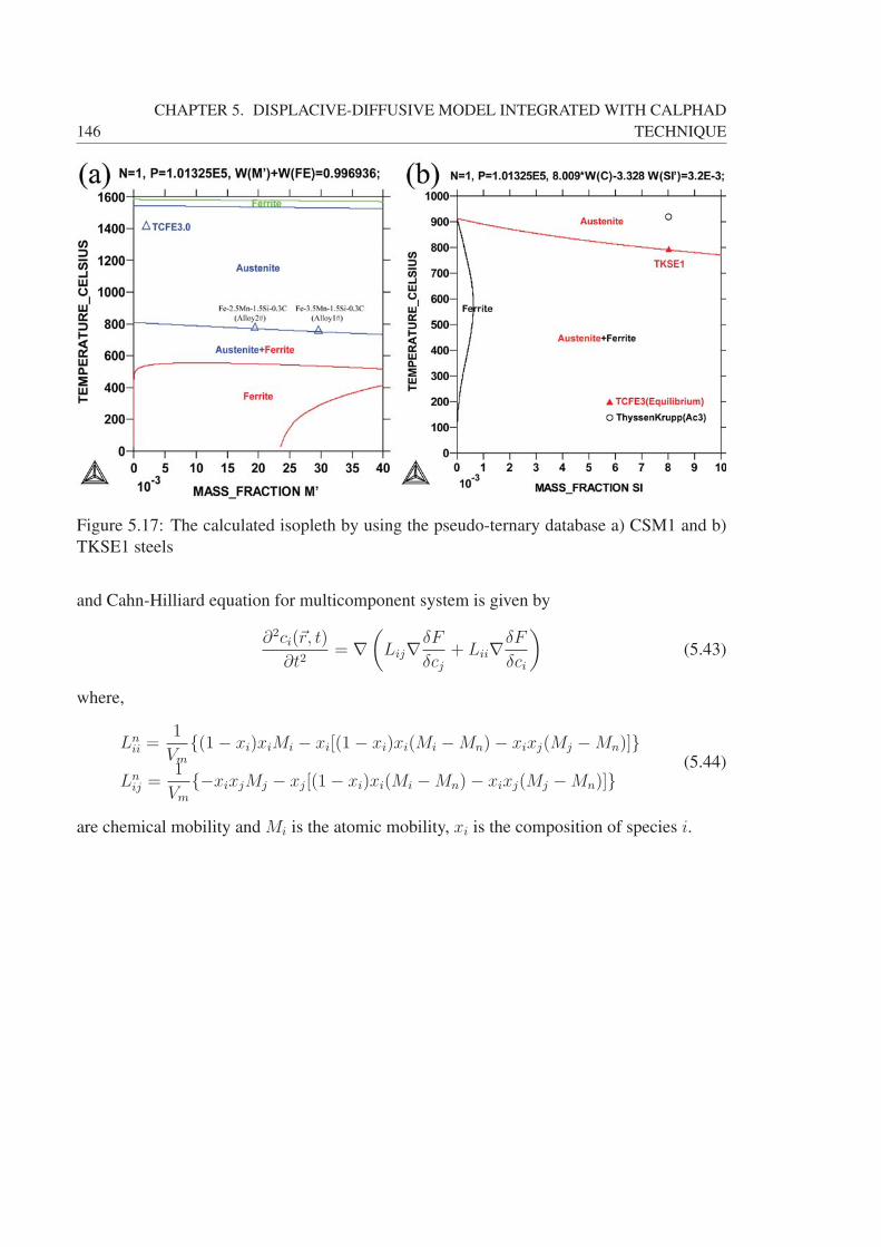
146
CHAPTER 5. DISPLACIVE-DIFFUSIVE MODEL INTEGRATED WITH CALPHAD
TECHNIQUE
Figure 5.17: The calculated isopleth by using the pseudo-ternary database a) CSM1 and b)
TKSE1 steels
and Cahn-Hilliard equation for multicomponent system is given by
∂2ci(�r, t)
∂t2= ∇
(Lij∇δF
δcj+ Lii∇δF
δci
)(5.43)
where,
Lnii =
1
Vm
{(1− xi)xiMi − xi[(1− xi)xi(Mi −Mn)− xixj(Mj −Mn)]}Ln
ij =1
Vm
{−xixjMj − xj[(1− xi)xi(Mi −Mn)− xixj(Mj −Mn)]}(5.44)
are chemical mobility and Mi is the atomic mobility, xi is the composition of species i.
Chapter 6Multi-field Model IncorporatingDislocations
-Origin of the Martensitic Morphology in Steels
The greatest shortcoming is that the dislocation density tensor, no matter whetherintroduced through differential geometry or in the conventional way, measures the average
dislocation density only and therefore, regards the internal mechanical state utmostincompletely.
-Ekkehard Kröner 1999
In chapter 5, the simulated zig-zag patterns of martensite plates have always been ob-
served in nickel carbon steel. However, the martensites in low- and medium-carbon steels
showing up different morphology have not been correctly simulated. In the perspective of
PTMC [Bha03], the {225}fcc habit plane in low- and medium-carbon steels is not an undis-
torted habit plane in the strictest sense, while {259}fcc habit plane in nickel steels is less dis-
torted than {225}fcc. Experimental results reveal the varying trend of habit plane {111}fcc→{225}fcc →{259}fcc with increasing carbon content as well as a decreasing of disloca-
tion density [Nis12]. To this end, it is a manifest that the configuration and evolution of
dislocations in solid crystals play a critical role in the development of various martensitic
morphology. Numerous research works on dislocations have been carried out in different
perspectives of energetics, kinematics and dynamics. Among them, the continuum theo-
ries of dislocations found by Kröner [Kro71] and Kosevich et al. [Kos64] and consolidated
by Le[LS96, KL08], Acharya [Ach01], Berdichevsky [Ber06], and Gurtin [Gur02], et al.
adopted the variables of dislocation density tensors as the functional of plastic deformation
to describe the dislocation patterning. For example, Kratochvíl and Sedlácek et al. for-
mulated the Eulerian and the Lagrangian frames based on the dislocation density tensor to
148 CHAPTER 6. MULTI-FIELD MODEL INCORPORATING DISLOCATIONS
evolve the dislocation patterning [KS03]. Rickman and Viñals [RV97] developed a general
phase-field formalism of the dislocation patterning by minimizing the free energy to obtain
the time-evolving dislocation density tensor, without considering the specific crystal struc-
tural symmetry. Limkumnerd and Sethna [LS06] proposed an elasto-plastic Landau model in
mesoscale to investigate the evolution of dislocations into sharp dislocation walls. The time
evolution of the system was implemented by using motion equations with the free energy
of the system written in pure plastic distortion tensor. The dislocation density tensor was
expressed in plastic distortion tensor by definition. The approach allows to study dislocation
motion by pure glide and a combination of glide and climb at different temperatures. These
models incorporated the concepts of incompatibility, energy minimization and energy dissi-
pation in solid crystals, showing many common ingredients between the continuum theories
of dislocations and the nonlinear Landau model. The high similarity inspires the initiatives
of integrating these two theories to shed light on the physical mechanisms of the interplaying
of dislocations and phase transformations, which gives rise to the formation of microstruc-
ture. Recently, Gröger utilized Kröner’s continuum theory to deal with the formation of
distinct microstructure in a MT affected by the dislocations [GLS08, GLS10]. The pres-
ence and evolution of dislocations were depicted as the response to the nonlocal coupling
of the incompatibility field and the OP strains. The incompatibility was explicitly written
as the dual-curl of elastic strain tensor and related to the gradients of the scalar dislocation
density. Minimizing the free energy subject to the incompatibility constraint for a given
distribution of dislocations generated a localized stress field that exerted effects on the for-
mation of martensite variant. Combining the methods of Gröger and Limkumnerd allows us
to propose the Landau model of MT with dislocations in Lagrange dynamics in this chapter.
Instead of the explicitly embedding incompatibility into TDGL equation in Gröger’s work,
our model characterizes in the usage of the underdamped general equation of motion with
basic variables of displacements or velocities. So it also avoids the derivation of the complex
incompatibility tensor when the model is extended to 3D.
6.1 Continuum Theory of Dislocations
The dislocation deformation viewed in macroscopic continuum has a general property
that there is a certain finite displacement increment b with the same magnitude and direction
as one of the lattice vectors when calculating the net displacement u along a passage round
any closed contour L, which encloses the dislocation line with the direction unit vector τ ,
see Figure 6.1.
The property of a single dislocation with Burgers vector b can be described as the integral
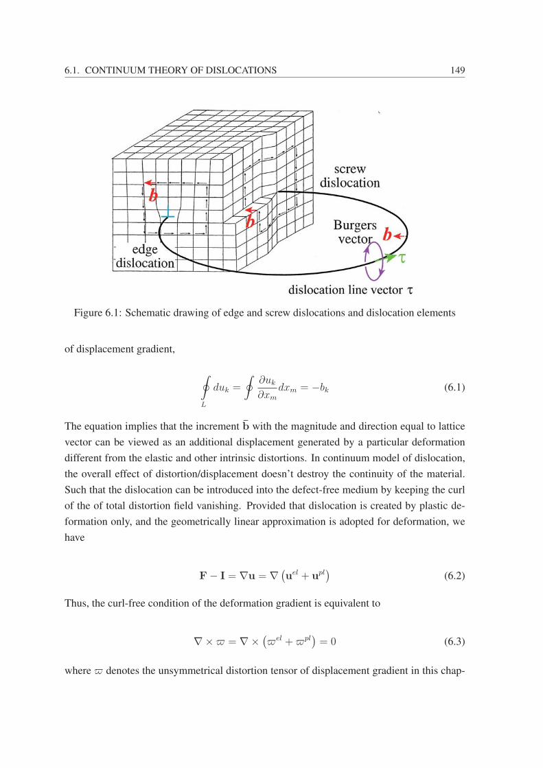
6.1. CONTINUUM THEORY OF DISLOCATIONS 149
Figure 6.1: Schematic drawing of edge and screw dislocations and dislocation elements
of displacement gradient,
∮L
duk =
∮∂uk
∂xm
dxm = −bk (6.1)
The equation implies that the increment b with the magnitude and direction equal to lattice
vector can be viewed as an additional displacement generated by a particular deformation
different from the elastic and other intrinsic distortions. In continuum model of dislocation,
the overall effect of distortion/displacement doesn’t destroy the continuity of the material.
Such that the dislocation can be introduced into the defect-free medium by keeping the curl
of the of total distortion field vanishing. Provided that dislocation is created by plastic de-
formation only, and the geometrically linear approximation is adopted for deformation, we
have
F− I = ∇u = ∇ (uel + upl)
(6.2)
Thus, the curl-free condition of the deformation gradient is equivalent to
∇×� = ∇× (�el +�pl)= 0 (6.3)
where � denotes the unsymmetrical distortion tensor of displacement gradient in this chap-
150 CHAPTER 6. MULTI-FIELD MODEL INCORPORATING DISLOCATIONS
ter, i.e.
�mk =∂uk
∂xm
, εmk =1
2(�km +�mk) (6.4)
Utilizing Stokes’ theorem, dxm ∼ εilmdfi∂∂xl
, the integral round the contour L can be trans-
formed into a surface integral SL with the unit surface fi. Thus, Eq.(6.1) is rewritten as
∮L
duplk =
∮L
�plmkdxm =
∮SL
εilm∂�pl
mk
∂xl
dfi = −bk (6.5)
Here, the integral over the surface has nonvanishing values only along the singular disloca-
tion line, such that the integral must be solved by mean of delta function.
εilm∂2upl
k
∂xm∂xl
= −τibkδ (ξ) (6.6)
Now we derive the force on the dislocation due to the local elastic stress created by
external loading. Let an element dislocation τdl be displaced by an amount δx , the area
change of the dislocation loop is
δs = δx× τdl, i.e. δsk = εklmδxlτmdl (6.7)
In general, the work δW done by elastic stress in an infinitesimal displacement can be ex-
pressed as
δW =
∫σikδε
plikdV =
∫flδxldl (6.8)
In the case of slip, the very elastic stress creates the displacement increment (Burgers vector)
of b between both sides of the slip plane. Therefore, the work is
δW = biδ
∫σikdsk = bi
∫σikεklmδxlτmdl (6.9)
Substituting the expression of unit area Eq.(6.7) into Eq.(6.9), the Peach-Koehler equation is
derived
fl = εlkmσkibiτm, f = (σ · b)× τ (6.10)
Again with the property of the discontinuity represented by b on an arbitrarily chosen
surface spanning the dislocation loop, the displacement gradient and strain tensors due to the

6.1. CONTINUUM THEORY OF DISLOCATIONS 151
dislocation are written in a form similar to the strain kinematic compatibility (Eq. 2.72) in
conventional phase field method but including a delta singularity.
εplik =1
2(nibk + nkbi) δ (ξ)
�plik = nibkδ (ξ)
(6.11)
where ni is the component of slip plane normal.
Except for the above variables are in common with elasticity, several variables frequently
used in continuum theory of dislocations are introduced. One is the dislocation density tensor
describing the distribution of dislocation
εilm∂�pl
mk
∂xl
= −ρik (6.12)
An integral of ρik over a surface S spanning any contour is equal to sum of the Burgers
vectors b for all the dislocation lines embraced by the contour∫SL
ρikdsi = bk (6.13)
With Eqs. (6.11) and (6.12) , the dislocation density tensor of a single dislocation reads
ρik = τibkδ (ξ) (6.14)
The dislocation density tensor ρik served as the state function is independent of whether
the dislocations are at rest or motion. To describe the time evolution of the dislocation, the
dislocation flux density tensor has to be introduced as follow
−jik =∂�pl
ik
∂t(6.15)
By applying right-hand rule ni = (−τ × δx)i, we can derive the flux density tensor for an
isolate dislocation
jik = −∂�plik
∂t= −∂nibkδ (ξ)
∂t= −εilm∂xlτmbkδ (ξ)
∂t= εilmρlkvm
=εilmτl∂xmbkδ (ξ)
∂t= εilmτlvmbkδ (ξ)
(6.16)
where v is the velocity of the moving dislocation line. It is worthy of note that the trace of
jik is proportional to the component of the velocity of dislocation along the normal of its slip
plane. If the trace of jkk = 0, the motion of the dislocation is conservatively slipping on the
slip plane without any inelastic volume changes generated. Otherwise, the motion contains
a non-conservative, vacancy/interstitial diffusion (climb) piece.
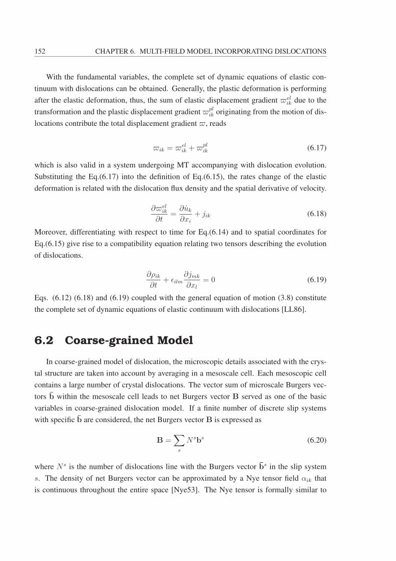
152 CHAPTER 6. MULTI-FIELD MODEL INCORPORATING DISLOCATIONS
With the fundamental variables, the complete set of dynamic equations of elastic con-
tinuum with dislocations can be obtained. Generally, the plastic deformation is performing
after the elastic deformation, thus, the sum of elastic displacement gradient �elik due to the
transformation and the plastic displacement gradient �plik originating from the motion of dis-
locations contribute the total displacement gradient �, reads
�ik = �elik +�pl
ik (6.17)
which is also valid in a system undergoing MT accompanying with dislocation evolution.
Substituting the Eq.(6.17) into the definition of Eq.(6.15), the rates change of the elastic
deformation is related with the dislocation flux density and the spatial derivative of velocity.
∂�elik
∂t=
∂uk
∂xi
+ jik (6.18)
Moreover, differentiating with respect to time for Eq.(6.14) and to spatial coordinates for
Eq.(6.15) give rise to a compatibility equation relating two tensors describing the evolution
of dislocations.
∂ρik∂t
+ εilm∂jmk
∂xl
= 0 (6.19)
Eqs. (6.12) (6.18) and (6.19) coupled with the general equation of motion (3.8) constitute
the complete set of dynamic equations of elastic continuum with dislocations [LL86].
6.2 Coarse-grained Model
In coarse-grained model of dislocation, the microscopic details associated with the crys-
tal structure are taken into account by averaging in a mesoscale cell. Each mesoscopic cell
contains a large number of crystal dislocations. The vector sum of microscale Burgers vec-
tors b within the mesoscale cell leads to net Burgers vector B served as one of the basic
variables in coarse-grained dislocation model. If a finite number of discrete slip systems
with specific b are considered, the net Burgers vector B is expressed as
B =∑s
N sbs (6.20)
where N s is the number of dislocations line with the Burgers vector bs in the slip system
s. The density of net Burgers vector can be approximated by a Nye tensor field αik that
is continuous throughout the entire space [Nye53]. The Nye tensor is formally similar to
6.2. COARSE-GRAINED MODEL 153
Figure 6.2: Schematic illustration of the mesoscopic cell is represented in the entire solid
black square, in which many crystallographic FCC unit cells are outlined in grey ; the slip
planes (dotted lines in blue and red) correspond to two {110} slip systems.
the dislocation density ρik representing the net length of all dislocation lines per area of the
mesoscale cell in this work.
∇×�pl = εilm∂�pl
mk
∂xl
= −αik =∑s
Dsτ si bsk (6.21)
where Ds is the scalar dislocation density representing the number of dislocation lines of slip
system s per unit area. In line with αik, the mesoscale flux density tensor J is defined as
Jik =∑s
Dsεilmτsl v
smb
sk (6.22)
In our coarse-grained model coupling MT and dislocations, the complete set of dynamic
equations, i.e. Eqs. (3.8), (6.12), (6.18) and (6.19), is not rigidly followed for simplicity.
The general equation of motion is still used to evolve the total displacement and to dissipate
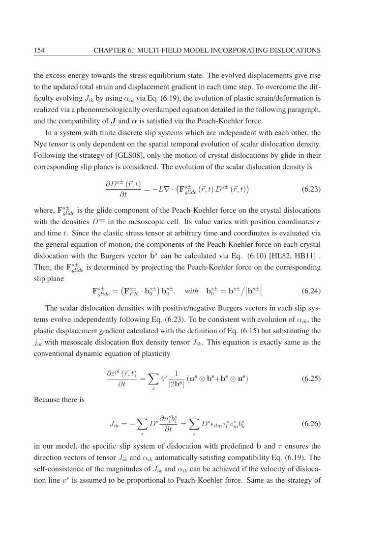
154 CHAPTER 6. MULTI-FIELD MODEL INCORPORATING DISLOCATIONS
the excess energy towards the stress equilibrium state. The evolved displacements give rise
to the updated total strain and displacement gradient in each time step. To overcome the dif-
ficulty evolving Jik by using αik via Eq. (6.19), the evolution of plastic strain/deformation is
realized via a phenomenologically overdamped equation detailed in the following paragraph,
and the compatibility of J and α is satisfied via the Peach-Koehler force.
In a system with finite discrete slip systems which are independent with each other, the
Nye tensor is only dependent on the spatial temporal evolution of scalar dislocation density.
Following the strategy of [GLS08], only the motion of crystal dislocations by glide in their
corresponding slip planes is considered. The evolution of the scalar dislocation density is
∂Ds± (�r, t)
∂t= −L∇ · (Fs±
glide (�r, t)Ds± (�r, t)
)(6.23)
where, Fs±glide is the glide component of the Peach-Koehler force on the crystal dislocations
with the densities Ds± in the mesoscopic cell. Its value varies with position coordinates r
and time t. Since the elastic stress tensor at arbitrary time and coordinates is evaluated via
the general equation of motion, the components of the Peach-Koehler force on each crystal
dislocation with the Burgers vector bs can be calculated via Eq. (6.10) [HL82, HB11] .
Then, the Fs±glide is determined by projecting the Peach-Koehler force on the corresponding
slip plane
Fs±glide =
(Fs±
PK · bs±0
)bs±0 , with bs±
0 = bs±/∣∣bs±∣∣ (6.24)
The scalar dislocation densities with positive/negative Burgers vectors in each slip sys-
tems evolve independently following Eq. (6.23). To be consistent with evolution of αik, the
plastic displacement gradient calculated with the definition of Eq. (6.15) but substituting the
jik with mesoscale dislocation flux density tensor Jik. This equation is exactly same as the
conventional dynamic equation of plasticity
∂εpl (�r, t)
∂t=∑s
γs 1
|2bs| (ns ⊗ bs+bs ⊗ ns) (6.25)
Because there is
Jik = −∑s
Ds∂nsi b
si
∂t=∑s
Dsεilmτsl v
smb
sk (6.26)
in our model, the specific slip system of dislocation with predefined b and τ ensures the
direction vectors of tensor Jik and αik automatically satisfing compatibility Eq. (6.19). The
self-consistence of the magnitudes of Jik and αik can be achieved if the velocity of disloca-
tion line vs is assumed to be proportional to Peach-Koehler force. Same as the strategy of
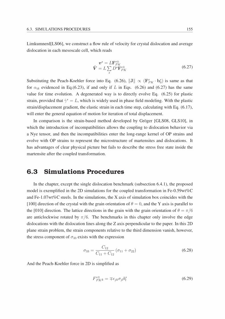
6.3. SIMULATIONS PROCEDURES 155
Limkumnerd[LS06], we construct a flow rule of velocity for crystal dislocation and average
dislocation in each mesoscale cell, which reads
vs = LFs±PK
V = L∑s
DsFs±PK
(6.27)
Substituting the Peach-Koehler force into Eq. (6.26), ‖J‖ ∝ (FsPK · bs
0) is same as that
for αik evidenced in Eq.(6.23), if and only if L in Eqs. (6.26) and (6.27) has the same
value for time evolution. A degenerated way is to directly evolve Eq. (6.25) for plastic
strain, provided that γs = L, which is widely used in phase field modeling. With the plastic
strain/displacement gradient, the elastic strain in each time step, calculating with Eq. (6.17),
will enter the general equation of motion for iteration of total displacement.
In comparison is the strain-based method developed by Gröger [GLS08, GLS10], in
which the introduction of incompatibilities allows the coupling to dislocation behavior via
a Nye tensor, and then the incompatibilities enter the long-range kernel of OP strains and
evolve with OP strains to represent the microstructure of martensites and dislocations. It
has advantages of clear physical picture but fails to describe the stress free state inside the
martensite after the coupled transformation.
6.3 Simulations Procedures
In the chapter, except the single dislocation benchmark (subsection 6.4.1), the proposed
model is exemplified in the 2D simulations for the coupled transformation in Fe-0.59wt%C
and Fe-1.07wt%C steels. In the simulations, the X axis of simulation box coincides with the
[100] direction of the crystal with the grain orientation of θ = 0, and the Y axis is parallel to
the [010] direction. The lattice directions in the grain with the grain orientation of θ = π/6
are anticlockwise rotated by π/6. The benchmarks in this chapter only involve the edge
dislocations with the dislocation lines along the Z axis perpendicular to the paper. In this 2D
plane strain problem, the strain components relative to the third dimension vanish, however,
the stress component of σ33 exists with the expression
σ33 =C12
C11 + C12
(σ11 + σ22) (6.28)
And the Peach-Koehler force in 2D is simplified as
F s±PKk = ∓εjkσjlb
sl (6.29)

156 CHAPTER 6. MULTI-FIELD MODEL INCORPORATING DISLOCATIONS
in the numerical implementation of Eqs. (6.23) and (6.24). For simplicity, we consider
only two slip systems in a FCC austenite with the Burgers vectors of1
2< 110 >, which
are evidenced as the active mode of glide accounting for plastic deformation in experiments
[MHF+06, IMTK11]. Since each slip system contains crystal dislocations with positive and
negative Burgers vectors, the scalar densities of these dislocations have to be treated sepa-
rately. For specific, four independent scalar dislocation densities correspond to the Burgers
vectors of b1± = ±1/2[110] and b2± = ±1/2[110], respectively. Figure 6.2 shows the
schematic illustration of the dislocation configuration used in our benchmarks. In numerical
simulations, most of the materials and simulation parameters are chosen the same as those
in chapter 5. The scalar dislocation density ranging 0 to 6 ∗ 1015m−2 is given with different
values for simulations. The Onsager coefficient in L in overdamped equations is set to 1.
Other parameters will be given in the discussion of the microstructure results.
6.4 Microstructure Simulations
6.4.1 Evolution of Single Edge Dislocation
In order to demonstrate that our model is capable of describing the internal stress field
around individual net dislocations by solving the set of modified motion equations, a bench-
mark for the stress field evolution with a single edge dislocation was carried out. The edge
dislocation embedded in an isotropic austenite has dislocation line along the Z axis perpen-
dicular to the paper, and Burgers vector directs toward the X axis. From the Figure 6.3 (a)
and (b), the overall distribution of the calculated stress field around the edge dislocation is
similar to that derived from the isotropic elasticity [HL82, HB11]. However, the stress fields
of the dislocations will be altered when the evolution of dislocation is coupled with MT, es-
pecially when dislocations are located at interfaces, such as grain boundaries, habit planes,
etc., where the stresses raised by MT cannot be thoroughly eliminated. Figure 6.3(c) and (d)
show the morphology of martensites represented by the deviatoric strain e2 and the devia-
toric stress σ2 undergoing a square-to-rectangular MT. The characteristic deviatoric strain e2
of the lattice caused by an edge dislocation in the middle of the block is similar to the strain
based TDGL results of [GLS08, GLS10]. However, our simulated stress field shows the in-
ternal stress is only accumulated around the dislocation, while a stress-free state is found in
the interior parts of the perfectly formed martensite variants. It significantly differs from the
strain-based scenario [GLS08].
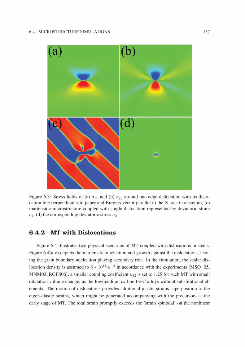
6.4. MICROSTRUCTURE SIMULATIONS 157
Figure 6.3: Stress fields of (a) σxx and (b) σyy around one edge dislocation with its dislo-
cation line perpendicular to paper and Burgers vector parallel to the X axis in austenite; (c)
martensitic microstructure coupled with single dislocation represented by deviatoric strain
e2; (d) the corresponding deviatoric stress σ2
6.4.2 MT with Dislocations
Figure 6.4 illustrates two physical scenarios of MT coupled with dislocations in steels.
Figure 6.4(a-c) depicts the martensitic nucleation and growth against the dislocations, leav-
ing the grain boundary nucleation playing secondary role. In the simulation, the scalar dis-
location density is assumed to 6 ∗ 1014m−2 in accordance with the experiments [MSO+05,
MNM03, RGFS06]; a smaller coupling coefficient κ12 is set to 1.25 for such MT with small
dilatation volume change, as the low/medium carbon Fe-C alloys without substitutional el-
ements. The motion of dislocations provides additional plastic strains superposition to the
eigen-elastic strains, which might be generated accompanying with the precursors at the
early stage of MT. The total strain promptly exceeds the ’strain spinodal’ on the nonlinear
158 CHAPTER 6. MULTI-FIELD MODEL INCORPORATING DISLOCATIONS
nonlocal energy surface, such that the intragranular nucleation precedes the grain boundary
nucleation as is shown in Figure 6.4(b). Finally, the mixed microstructure with martensite
and retained austenite is formed and characterized by the rougher twin boundary compared
with sharp interface discovered in SMA. It is the most remarkable difference on morphology
of martensites between SMAs and steels. A few of noticable retained austenites represented
in green are found to locate at twin boundaries, inside the martensite variants and in the
regions surrounded by martensite package, as is shown in Figure 6.4(c).
Figure 6.4: MT in polycrystalline Fe-0.59wt.%C alloy coupled with the evolution of dislo-
cation (scalar dislocation density 6 ∗ 1014m−2) with κ12 = 1.25 (a-c) and κ12 = 4.0 (d-f).
Figure 6.4(d-f) depicts another scenario of the grain boundary nucleation and growth
surpassing the dislocation nucleation due to the large lattice-misfit strain introduced by
κ12 = 4.25. In this simulation, the effect of dilatational volume change on the marten-
site morphology is also evidenced by the higher volume fraction of retained austenite and
the butterfly like martensite variants in the grains, as apparently seen from the simulated
microstructure of Fe-1.07wt.% C in Figure 6.5(d-f). Although the alloying elements are not
included in simulation, the simulated microstructure well represents the typical appearance
of martensites in high alloying steels, which implies that the alloying elements play their
rules more via the geometry rather than the chemistry. The similar stories are also found in
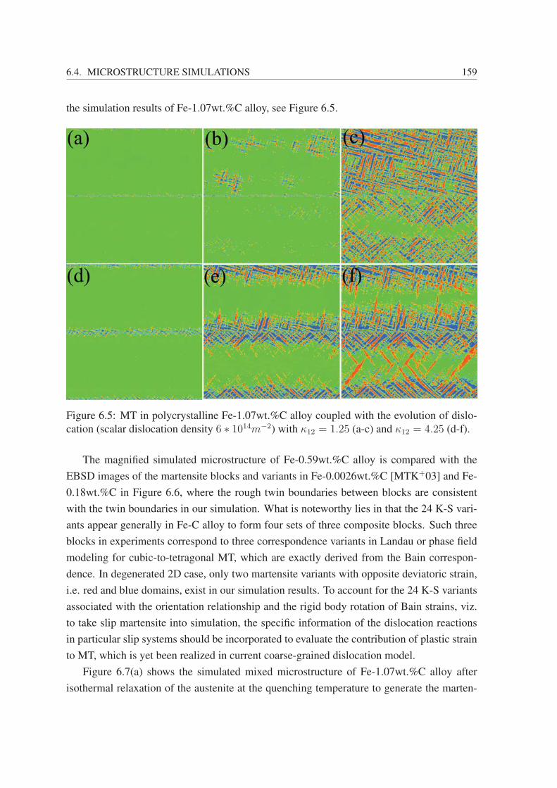
6.4. MICROSTRUCTURE SIMULATIONS 159
the simulation results of Fe-1.07wt.%C alloy, see Figure 6.5.
Figure 6.5: MT in polycrystalline Fe-1.07wt.%C alloy coupled with the evolution of dislo-
cation (scalar dislocation density 6 ∗ 1014m−2) with κ12 = 1.25 (a-c) and κ12 = 4.25 (d-f).
The magnified simulated microstructure of Fe-0.59wt.%C alloy is compared with the
EBSD images of the martensite blocks and variants in Fe-0.0026wt.%C [MTK+03] and Fe-
0.18wt.%C in Figure 6.6, where the rough twin boundaries between blocks are consistent
with the twin boundaries in our simulation. What is noteworthy lies in that the 24 K-S vari-
ants appear generally in Fe-C alloy to form four sets of three composite blocks. Such three
blocks in experiments correspond to three correspondence variants in Landau or phase field
modeling for cubic-to-tetragonal MT, which are exactly derived from the Bain correspon-
dence. In degenerated 2D case, only two martensite variants with opposite deviatoric strain,
i.e. red and blue domains, exist in our simulation results. To account for the 24 K-S variants
associated with the orientation relationship and the rigid body rotation of Bain strains, viz.
to take slip martensite into simulation, the specific information of the dislocation reactions
in particular slip systems should be incorporated to evaluate the contribution of plastic strain
to MT, which is yet been realized in current coarse-grained dislocation model.
Figure 6.7(a) shows the simulated mixed microstructure of Fe-1.07wt.%C alloy after
isothermal relaxation of the austenite at the quenching temperature to generate the marten-
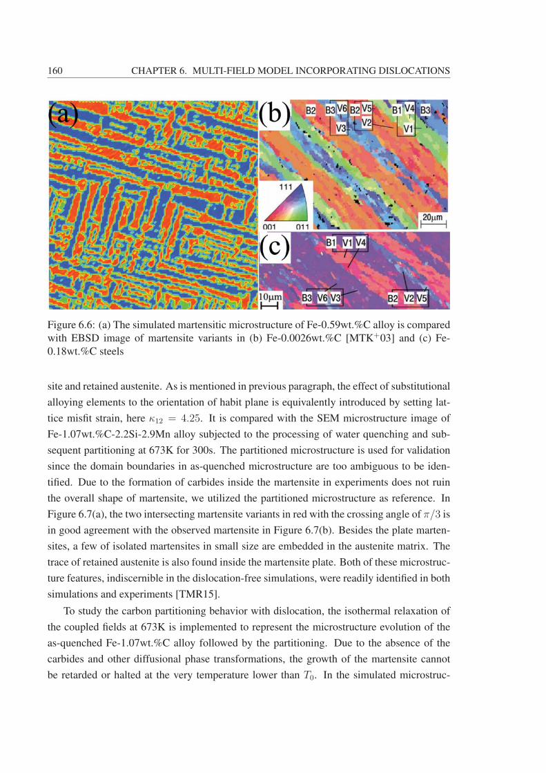
160 CHAPTER 6. MULTI-FIELD MODEL INCORPORATING DISLOCATIONS
Figure 6.6: (a) The simulated martensitic microstructure of Fe-0.59wt.%C alloy is compared
with EBSD image of martensite variants in (b) Fe-0.0026wt.%C [MTK+03] and (c) Fe-
0.18wt.%C steels
site and retained austenite. As is mentioned in previous paragraph, the effect of substitutional
alloying elements to the orientation of habit plane is equivalently introduced by setting lat-
tice misfit strain, here κ12 = 4.25. It is compared with the SEM microstructure image of
Fe-1.07wt.%C-2.2Si-2.9Mn alloy subjected to the processing of water quenching and sub-
sequent partitioning at 673K for 300s. The partitioned microstructure is used for validation
since the domain boundaries in as-quenched microstructure are too ambiguous to be iden-
tified. Due to the formation of carbides inside the martensite in experiments does not ruin
the overall shape of martensite, we utilized the partitioned microstructure as reference. In
Figure 6.7(a), the two intersecting martensite variants in red with the crossing angle of π/3 is
in good agreement with the observed martensite in Figure 6.7(b). Besides the plate marten-
sites, a few of isolated martensites in small size are embedded in the austenite matrix. The
trace of retained austenite is also found inside the martensite plate. Both of these microstruc-
ture features, indiscernible in the dislocation-free simulations, were readily identified in both
simulations and experiments [TMR15].
To study the carbon partitioning behavior with dislocation, the isothermal relaxation of
the coupled fields at 673K is implemented to represent the microstructure evolution of the
as-quenched Fe-1.07wt.%C alloy followed by the partitioning. Due to the absence of the
carbides and other diffusional phase transformations, the growth of the martensite cannot
be retarded or halted at the very temperature lower than T0. In the simulated microstruc-
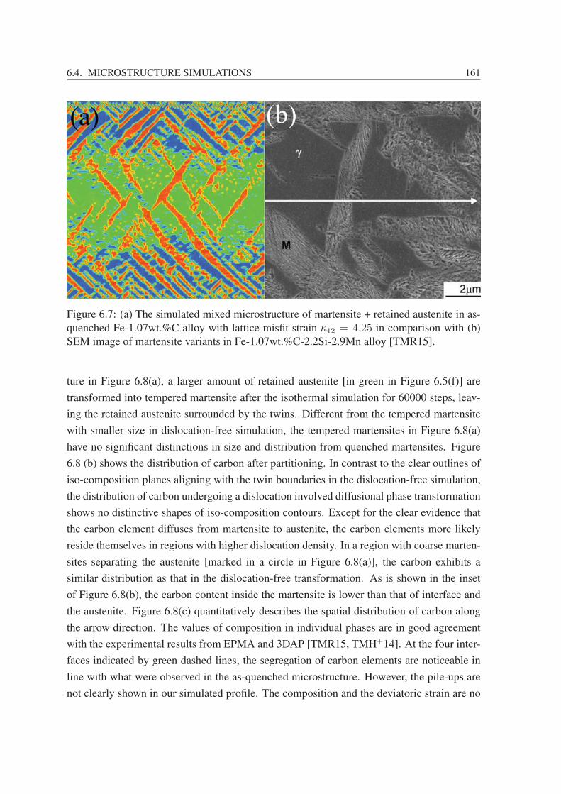
6.4. MICROSTRUCTURE SIMULATIONS 161
Figure 6.7: (a) The simulated mixed microstructure of martensite + retained austenite in as-
quenched Fe-1.07wt.%C alloy with lattice misfit strain κ12 = 4.25 in comparison with (b)
SEM image of martensite variants in Fe-1.07wt.%C-2.2Si-2.9Mn alloy [TMR15].
ture in Figure 6.8(a), a larger amount of retained austenite [in green in Figure 6.5(f)] are
transformed into tempered martensite after the isothermal simulation for 60000 steps, leav-
ing the retained austenite surrounded by the twins. Different from the tempered martensite
with smaller size in dislocation-free simulation, the tempered martensites in Figure 6.8(a)
have no significant distinctions in size and distribution from quenched martensites. Figure
6.8 (b) shows the distribution of carbon after partitioning. In contrast to the clear outlines of
iso-composition planes aligning with the twin boundaries in the dislocation-free simulation,
the distribution of carbon undergoing a dislocation involved diffusional phase transformation
shows no distinctive shapes of iso-composition contours. Except for the clear evidence that
the carbon element diffuses from martensite to austenite, the carbon elements more likely
reside themselves in regions with higher dislocation density. In a region with coarse marten-
sites separating the austenite [marked in a circle in Figure 6.8(a)], the carbon exhibits a
similar distribution as that in the dislocation-free transformation. As is shown in the inset
of Figure 6.8(b), the carbon content inside the martensite is lower than that of interface and
the austenite. Figure 6.8(c) quantitatively describes the spatial distribution of carbon along
the arrow direction. The values of composition in individual phases are in good agreement
with the experimental results from EPMA and 3DAP [TMR15, TMH+14]. At the four inter-
faces indicated by green dashed lines, the segregation of carbon elements are noticeable in
line with what were observed in the as-quenched microstructure. However, the pile-ups are
not clearly shown in our simulated profile. The composition and the deviatoric strain are no
162 CHAPTER 6. MULTI-FIELD MODEL INCORPORATING DISLOCATIONS
longer homogeneous inside the martensites due to the existence of dislocations, which has
also been evidenced by experiments.
6.4.3 Limitation of the Model
Although our multi-fields model has ability to represent the stress field of dislocation and
account for many experimental observations in viewpoint of interplaying of dislocation and
transformation strain, our modified coarse-grained dislocation model is yet embryonic. The
greatest shortcoming is that the Nye tensor measures the average dislocation density only
and therefore regards the internal mechanical state utmost incompletely. Many features,
like more complicated cross slip systems, dislocation tangling, yield surfaces, nucleation of
new dislocations, etc., which are known to be macroscopically important in real materials,
have been ignored in our model. While, it does incorporate the geometric constraints, long-
range elastic interaction, and energetics driving the dislocation dynamics, but the dynamics
remains suffering from many hypothesis. Therefore, it is yet developed into a mature method
in comparison with the strain based dynamics driven by minimizing energy with a clear
statement of incompatibility in geometry.
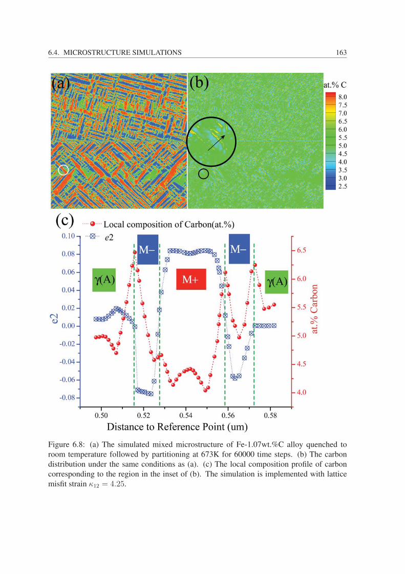
6.4. MICROSTRUCTURE SIMULATIONS 163
Figure 6.8: (a) The simulated mixed microstructure of Fe-1.07wt.%C alloy quenched to
room temperature followed by partitioning at 673K for 60000 time steps. (b) The carbon
distribution under the same conditions as (a). (c) The local composition profile of carbon
corresponding to the region in the inset of (b). The simulation is implemented with lattice
misfit strain κ12 = 4.25.

164 CHAPTER 6. MULTI-FIELD MODEL INCORPORATING DISLOCATIONS
Chapter 7Conclusions and Future Works
If we knew what it was we were doing, it would not be called research, would it?
-Albert Einstein
7.1 Conclusions
This thesis has provided deeper insights into the physical essentials of the various models
of MTs and the Landau model of MT has been extended to be used in practical applications
of engineering materials.
The comparison of the current models of MT led to the conclusion that, the models, rather
than being isolated, share many common ingredients while cast their pronounced individual
distinctiveness, and none of them is applicable to every aspect of the MT.
• Regarding the physical essentials of MT models
(1) All the models are common in energy minimization, either explicitly or implicitly;
(2) PTMCs and phase field models have a foundation on rigid body mechanics, while
the Landau model is rooted in wave mechanics and crystal lattice dynamics;
(3) The microelasticity phase field and Landau models resort to Green’s function based
long-range integral kernel in Fourier space to represent the symmetry constraint on
martensite microstructure, while the PTMC and thermomechanical phase field directly
handle the kinematic compatibility and transformation strain in coordinate space;
(4) The Landau model equipped with finite strains, anharmonic and nonlocal energy in
the linearized tensor space, and inertial dynamics is the most complete from the physics
viewpoint and has ability to capture the complete dynamic behaviors of martensites.
• Regarding the application capabilities among the models,
166 CHAPTER 7. CONCLUSIONS AND FUTURE WORKS
(1) in thermodynamics, the PTMC and phase field methods- in contrast with the Lan-
dau model- has been widely used to study MTs coupled with various effects, includ-
ing grain boundaries and dislocations. They also have advantages in describing habit
plane, internal twinning and slip martensite. In this respect, the development of Landau
model falls behind them.
(2) in dynamics, the Landau model is able to tackle all dynamics, ranging from inertial
to full dissipative and from TDGL to statics, as such the phenomena due to the dy-
namics can readily be captured by Landau modeling. In contrast, the PTMC and phase
field methods are only sufficient in statics and dissipative dynamics for the equilibrium
microstructure and properties governed by dissipative dynamics.
To widen the applications of Landau model, it has been extended to analyze martensitic
nucleation and growth in polycrystals, coupled with diffusional transformations (through
integration with CALPHAD technique), and to incorporate the influence of dislocations. The
new model has been used to provide a deeper understanding of the complex microstructure
evolution during MTs in steels. In particular, the following objectives have been achieved:
• A modified Landau model was developed to describe the MTs in polycrystals based
on the Lagrange-Rayleigh dynamics with the Landau energetics. The stress term in the
dissipative force equation was reformulated in terms of the functional of local Landau energy
with respect to global displacement gradients. The key microstructural features and their
response to the external loads were in agreement with experimental observations and satisfied
the kinematic compatibility condition in CM-PTMC. Therefore, the physical consistence
between Landau model and CM-PTMC was identified and verified.
• The updated model was successfully applied to the martensitic nucleation problem in
polycrystals. The simulated results manifest that the MT undergoing a non-classical transfor-
mation path led to a new classical ’C-shaped’ relationship between the nucleation modes and
the processing parameters such as external loading and temperature. It implied that the clas-
sical transformation path indeed corresponds to a thermodynamic limit of the non-classical
paths.
• An attempt of semi-quantitative description for the displacive-diffusive coupled trans-
formation was made by integrating the nonlinear-nonlocal Landau model with CALPHAD
technique. The Landau free energy and the corresponding driving force were quantified
from the CALPHAD type thermodynamic database, whereas the chemical mobility were ex-
pressed in the functions of atomic mobility that was again from the diffusion kinetic database.
With the correct diffusion potential and real chemical mobility, the mechanism of partition-
ing of carbon in steels was proven an ordinary diffusion event governed by the diffusion
potential and chemical mobility, which varied spatially and temporally. The carbon diffused
7.2. FUTURE WORKS 167
from martensite to austenite as a natural result of the difference of the mobilities between
two phases.
• A simplified dislocation model based on the continuum theory was seamlessly ’embed-
ded in’ the Landau model of MTs. Together with the diffusional transformation model as a
whole, the multi-field model succeeded in simulating the dissipative MT in steel rather than
be limited in the SMAs or for functionalities only. Based on the simulations, the irregulari-
ties of microstructure, as rough twin boundaries and retained austenite within the martensite
in steels was attributed to the effect of dislocations.
7.2 Future Works
The following tasks are proposed in the further
• Development of the Bales-Gooding dynamic model with 3D long-range compatibility
kernel and 3D simulations for real materials with the combination of Landau energetics and
Bales-Gooding dynamics.
• Simulations of cubic-monoclinic II MTs by inertial dynamics.
• Extension of displacive-diffusive coupled transformation model to multicomponent and
multiphase system.
• Incorporation of nucleation of dislocations, slip systems, dislocation tangling to the
developed dislocation model in continuum theory.

168 CHAPTER 7. CONCLUSIONS AND FUTURE WORKS
Appendix ACompatibility Kernel ofCubic-Tetragonal MT

170 APPENDIX A. COMPATIBILITY KERNEL OF CUBIC-TETRAGONAL MT
Tab
leA
.1:
Com
pat
ibil
ity
ker
nel
of
cubic
-to-t
etra
gonal
MT
on
spec
ial
pla
nes
and
dir
ecti
ons
U22
U23
U23
kx�=
0,ky→
0,kz→
0
k2 x
2( k2 y
+k2 z
)N
2 yN
2 zk2 x
2( N2 y
+N
2 z
)√ 3k
2 x
2( k2 y
+k2 z
)√ 3N
2 yN
2 zk2 x
2( N2 y
+N
2 z
)3k
2 x
2( k2 y
+k2 z
)3N
2 yN
2 zk2 x
2( N2 y
+N
2 z
)ky�=
0,kx→
0,kz→
0
k2 y
2(k
2 x+k2 z)
N2 xN
2 zk2 y
2(N
2 x+N
2 z)
−√ 3k2 y
2(k
2 x+k2 z)
−√ 3N2 xN
2 zk2 y
2(N
2 x+N
2 z)
3k2 y
2(k
2 x+k2 z)
3N2 xN
2 zk2 y
2(N
2 x+N
2 z)
kz�=
0,kx→
0,ky→
0
2k2 z
( k2 x+k2 y
)2N
2 xN
2 yk2 z
( N2 x+N
2 y
)3( k2 x
−k2 y
)( k2 x
+k2 y
)3
0.5
0.5
kx�=
0,ky�=
0,kz→
0
1 2
( k2 y
k2 x
+k2 x
k2 y
) −1
√ 3 2
( k2 y
k2 x
−k2 x
k2 y
)3 2
( k2 y
k2 x
+k2 x
k2 y
) +5
kx�=
0,kz�=
0,ky→
012
( k2 x
k2 z
+4k
2 z
k2 x
+7)
−√ 3
2
( k2 x
k2 z
+3)
1 2
( 3k2 x
k2 z
+1)
kz�=
0,ky�=
0,kx→
0
1 2
( k2 x
k2 z
+4k
2 z
k2 x
+7)
√ 3 2
( k2 x
k2 z
+3)
1 2
( 3k2 x
k2 z
+1)

Appendix BCompatibility Kernel of Cubic-TrigonalMT
In cubic-to-trigonal MT, the non-OPs e1, e2, and e3 can be written in terms of OPs shear
strains
ei=1,2,3 =∑
s=4,5,6
Nises (B.1)
where, the matrix of Nis is
⎛⎝ N14 N15 N16
N24 N25 N26
N34 N35 N36
⎞⎠ =
⎛⎜⎜⎜⎜⎜⎜⎜⎝
(k2x − k2
y − k2z
)2√3O4
(k2y − k2
z − k2x
)2√3O5
(k2z − k2
x − k2y
)2√3O6(
k2x + k2
y
)2√2O4
− (k2x + k2
y
)2√2O5
− (k2x − k2
y
)2√2O6(
2k2z + k2
x − k2y
)2√6O4
(2k2
z − k2x + k2
y
)2√6O5
−(2k2
z + k2x + k2
y
)2√6O6
⎞⎟⎟⎟⎟⎟⎟⎟⎠
(B.2)
The harmonic energy of non-OP strains is reformulated as
fnon−OP =∑
i=1,2,3
Ai
2|ei (k)|
2
=∑
l,l′=4,5,6
A1
2Ul,l′ (k) el (k) e
∗l′ (k) (B.3)
Therefore, the compatibility kernel is derived
Ul,l′ (k) =υ
A1
∑i=1,2,3
AiNilNil′ (B.4)
Following the strategy in Subsection 2.4.11, the values of compatibility kernel at special
points in Fourier space are listed in Table B.1.
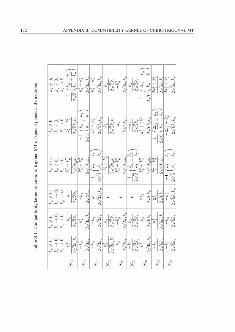
172 APPENDIX B. COMPATIBILITY KERNEL OF CUBIC-TRIGONAL MTT
able
B.1
:C
om
pat
ibil
ity
ker
nel
of
cubic
-to-t
rigonal
MT
on
spec
ial
pla
nes
and
dir
ecti
ons
kx�=
0,ky→
0,kz→
0
ky�=
0,kx→
0,kz→
0
kz�=
0,kx→
0,ky→
0
kx�=
0,ky�=
0,kz→
0
kx�=
0,kz�=
0,ky→
0
kz�=
0,ky�=
0,kx→
0
N14
k2 x
2√ 3kykz
−ky
2√ 3kz
−kz
2√ 3ky
k2 x−
k2 y
2√ 3kykz
k2 x−k2 z
2√ 3kykz
−1 2√ 3
( k y kz
+kz
ky
)
N15
−kx
2√ 3kz
k2 y
2√ 3kxkz
−kz
2√ 3kx
k2 x−
k2 y
2√ 3kxkz
−1 2√ 3
( k x kz
+kz
kx
)k2 y−
k2 z
2√ 3kxkz
N16
−kx
2√ 3ky
−ky
2√ 3kx
k2 z
2√ 3kxky
1
2√ 3
( k x ky
+ky
kx
)k2 z−k2 x
2√ 3kxky
k2 z−
k2 y
2√ 3kxky
N24
k2 x
2√ 2kykz
ky
2√ 2kz
0−k
2 x−k2 y
2√ 2kykz
k2 x
2√ 2kykz
ky
2√ 2kz
N25
−kx
2√ 2kz
−k2 y
2√ 2kxkz
0k2 x+k2 y
2√ 2kxkz
−kx
2√ 2kz
−k2 y
2√ 2kxkz
N26
−kx
2√ 2ky
ky
2√ 2kx
01
2√ 2
( k y kx
−kx ky
)−k
x
2√ 2ky
ky
2√ 2kx
N34
k2 x
2√ 6kykz
−ky
2√ 6kz
2kz
2√ 6ky
k2 y−k2 x
2√ 6kykz
k2 x+2k
2 z
2√ 6kykz
1
2√ 6
( 2kz
ky
−ky
kz
)
N35
−kx
2√ 6kz
k2 y
2√ 6kxkz
2kz
2√ 6kx
k2 x−
k2 y
2√ 6kxkz
1
2√ 6
( 2kz
kx
−kx kz
)2k
2 z+k2 y
2√ 6kxkz
N36
−kx
2√ 6ky
−ky
2√ 6kx
−k2 z
2√ 6kxky
−1 2√ 6
( k x ky
+ky
kx
)−2
k2 z−
k2 x
2√ 6kxky
2k2 z+k2 y
2√ 6kxky

Bibliography
[AA01] R Ahluwalia and G Ananthakrishna. Power-law statistics for avalanches in
a martensitic transformation. Physical Review Letters, 86(18):4076, 2001.
[ABKS78] I Ansara, C Bernard, L Kaufman, and P Spencer. A comparison of cal-
culated phase equilibria in selected ternary alloy systems using thermody-
namic values derived from different models. Calphad, 2(1):1–15, 1978.
[Ach01] A Acharya. A model of crystal plasticity based on the theory of contin-
uously distributed dislocations. Journal of the Mechanics and Physics of
Solids, 49(4):761–784, 2001.
[ADP66a] HI Aaronson, HA Domian, and GM Pound. Thermodynamics of the
austenite proeutectoid ferrite transformation. i. fe-c alloys. Transactions
of the Metallurgical Society of AIME, 236(5):753–767, 1966.
[ADP66b] HI Aaronson, HA Domian, and GM Pound. Thermodynamics of the
austenite proeutectoid ferrite transformation. ii. fe-c-x alloys. Transactions
of the Metallurgical Society of AIME, 236(5):768–781, 1966.
[Aiz69] K Aizu. Possible species of ferroelastic crystals and of simultaneously
ferroelectric and ferroelastic crystals. Journal of the Physical Society of
Japan, 27(2):387–396, 1969.
[AJK01] A Artemev, Y Jin, and AG Khachaturyan. Three-dimensional phase field
model of proper martensitic transformation. Acta Materialia, 49(7):1165–
1177, 2001.
[AJK02] A Artemev, YM Jin, and AG Khachaturyan. Three-dimensional phase
field model and simulation of cubic tetragonal martensitic transformation
in polycrystals. Philosophical Magazine A, 82(6):1249–1270, 2002.

174 BIBLIOGRAPHY
[AKV00] IS Aranson, VA Kalatsky, and VM Vinokur. Continuum field description
of crack propagation. Physical Review Letters, 85(1):118, 2000.
[ALS03] R Ahluwalia, T Lookman, and A Saxena. Elastic deformation of polycrys-
tals. Physical Review Letters, 91(5):055501, 2003.
[ALS06] R Ahluwalia, T Lookman, and A Saxena. Dynamic strain loading of cubic
to tetragonal martensites. Acta Materialia, 54(8):2109–2120, 2006.
[ALSA04] R Ahluwalia, T Lookman, A Saxena, and RC Albers. Landau theory for
shape memory polycrystals. Acta Materialia, 52(1):209–218, 2004.
[AQW15] R Ahluwalia, SS Quek, and DT Wu. Simulation of grain size effects
in nanocrystalline shape memory alloys. Journal of Applied Physics,
117(24):244305, 2015.
[BA06] M Bouville and R Ahluwalia. Interplay between diffusive and displacive
phase transformations: time-temperature-transformation diagrams and mi-
crostructures. Physical Review Letters, 97(5):055701, 2006.
[BA07] M Bouville and R Ahluwalia. Effect of lattice-mismatch-induced strains on
coupled diffusive and displacive phase transformations. Physical Review
B, 75(5):054110, 2007.
[Bal02] JM Ball. Some open problems in elasticity. In Geometry, mechanics, and
dynamics, pages 3–59. Springer, 2002.
[Bal04] JM Ball. Mathematical models of martensitic microstructure. Materials
Science and Engineering: A, 378(1):61–69, 2004.
[BB93] LA Bendersky and WJ Boettinger. Transformation of bcc and b2 high
temperature phases to hcp and orthorhombic structures in the ti-al-nb
system. part ii: Experimental tem study of microstructures. Journal of
Research-National Institute of Standards and Technology, 98:585–585,
1993.
[BBG98] L Bataillard, J-E Bidaux, and R Gotthardt. Interaction between microstruc-
ture and multiple-step transformation in binary niti alloys using in-situ
transmission electron microscopy observations. Philosophical Magazine
A, 78(2):327–344, 1998.

BIBLIOGRAPHY 175
[BC99] JM Ball and C Carstensen. Compatibility conditions for microstruc-
tures and the austenite–martensite transition. Materials Science and
Engineering: A, 273:231–236, 1999.
[BD24] EC Bain and NY Dunkirk. The nature of martensite. Transactions of the
Metallurgical Society of AIME, 70(1):25–47, 1924.
[Ber06] VL Berdichevsky. Continuum theory of dislocations revisited. Continuum
Mechanics and Thermodynamics, 18(3-4):195–222, 2006.
[BG91] GS Bales and RJ Gooding. Interfacial dynamics at a first-order phase tran-
sition involving strain: dynamical twin formation. Physical Review Letters,
67(24):3412, 1991.
[Bha91] K Bhattacharya. Wedge-like microstructure in martensites. Acta
Metallurgica et Materialia, 39(10):2431–2444, 1991.
[Bha03] K Bhattacharya. Microstructure of martensite: why it forms and how it
gives rise to the shape-memory effect, volume 2. Oxford University Press,
2003.
[BHK87] GR Barsch, B Horovitz, and JA Krumhansl. Dynamics of twin boundaries
in martensites. Physical Review Letters, 59(11):1251, 1987.
[BJ89] JM Ball and RD James. Fine phase mixtures as minimizers of energy. In
Analysis and Continuum Mechanics, pages 647–686. Springer, 1989.
[BK84] GR Barsch and JA Krumhansl. Twin boundaries in ferroelastic media with-
out interface dislocations. Physical Review Letters, 53(11):1069, 1984.
[BK88] GR Barsch and JA Krumhansl. Nonlinear and nonlocal continuum model
of transformation precursors in martensites. Metallurgical Transactions A,
19(4):761–775, 1988.
[BKB00] DN Bhate, A Kumar, and AF Bower. Diffuse interface model for electromi-
gration and stress voiding. Journal of Applied Physics, 87(4):1712–1721,
2000.
[BM54a] JS Bowles and JK Mackenzie. The crystallography of martensite transfor-
mations i. Acta Metallurgica, 2(1):129–137, 1954.

176 BIBLIOGRAPHY
[BM54b] JS Bowles and JK Mackenzie. The crystallography of martensite transfor-
mations iii. face-centred cubic to body-centred tetragonal transformations.
Acta Metallurgica, 2(2):224–234, 1954.
[Bro97] R Bro. Parafac. tutorial and applications. Chemometrics and Intelligent
Laboratory Systems, 38(2):149–171, 1997.
[BS05] K Bhattacharya and PM Suquet. A model problem concerning recoverable
strains of shape-memory polycrystals. In Proceedings of the Royal Society
of London A: Mathematical, Physical and Engineering Sciences, volume
461, pages 2797–2816. The Royal Society, 2005.
[BW96] TE Buchheit and JA Wert. Predicting the orientation-dependent stress-
induced transformation and detwinning response of shape memory alloy
single crystals. Metallurgical and Materials Transactions A, 27(2):269–
279, 1996.
[BYS+86] C Boulesteix, B Yangui, MB Salem, C Manolikas, and S Amelinckx.
The orientation of interfaces between a prototype phase and its ferroelas-
tic derivatives: theoretical and experimental study. Journal de Physique,
47(3):461–471, 1986.
[Cah59] JW Cahn. Free energy of a nonuniform system. ii. thermodynamic basis.
The Journal of Chemical Physics, 30(5):1121–1124, 1959.
[CC83] I-W Chen and Y-H Chiao. Martensitic nucleation in zro 2. Acta
Metallurgica, 31(10):1627–1638, 1983.
[CH58] JW Cahn and JE Hilliard. Free energy of a nonuniform system. i. interfacial
free energy. The Journal of Chemical Physics, 28(2):258–267, 1958.
[CH59] JW Cahn and JE Hilliard. Free energy of a nonuniform system. iii. nucle-
ation in a two-component incompressible fluid. The Journal of Chemical
Physics, 31(3):688–699, 1959.
[Che02] L-Q Chen. Phase-field models for microstructure evolution. Annual
Review of Materials Research, 32(1):113–140, 2002.
[Chr51] JW Christian. A theory of the transformation in pure cobalt. In Proceedings
of the Royal Society of London A: Mathematical, Physical and Engineering
Sciences, volume 206, pages 51–64. The Royal Society, 1951.

BIBLIOGRAPHY 177
[Chr02] JW Christian. The theory of transformations in metals and alloys. Newnes,
2002.
[Chu93] C Chu. Hysteresis and microstructures: a study of biaxial loading of com-
pound twins of cu–al–ni single crystals. Doctoral Dissertation University
of Minnesota, Minneapolis, MN, 1993.
[CILP12] J-Y Cho, AV Idesman, VI Levitas, and T Park. Finite element simula-
tions of dynamics of multivariant martensitic phase transitions based on
ginzburg–landau theory. International Journal of Solids and Structures,
49(14):1973–1992, 2012.
[CJ00] SH Curnoe and AE Jacobs. Twin wall of proper cubic-tetragonal ferroelas-
tics. Physical Review B, 62(18):R11925, 2000.
[CJ01a] SH Curnoe and AE Jacobs. Statics and dynamics of domain patterns in
hexagonal-orthorhombic ferroelastics. Physical Review B, 63(9):094110,
2001.
[CJ01b] SH Curnoe and AE Jacobs. Time evolution of tetragonal-orthorhombic
ferroelastics. Physical Review B, 64(6):064101, 2001.
[CK90] W Cao and JA Krumhansl. Continuum theory of 4mm-2mm proper fer-
roelastic transformation under inhomogeneous stress. Physical Review B,
42(7):4334, 1990.
[CKG90] W Cao, JA Krumhansl, and RJ Gooding. Defect-induced heterogeneous
transformations and thermal growth in athermal martensite. Physical
Review B, 41(16):11319, 1990.
[CKO+07] Y-W Cui, T Koyama, I Ohnuma, K Oikawa, R Kainuma, and K Ishida.
Simulation of hexagonal–orthorhombic phase transformation in polycrys-
tals. Acta Materialia, 55(1):233–241, 2007.
[Cla73] PC Clapp. A localized soft mode theory for martensitic transformations.
Physica Status Solidi (b), 57(2):561–569, 1973.
[Cla93] PC Clapp. Static and dynamic precursors of displacive transformations
near crystalline defects. Physica D: Nonlinear Phenomena, 66(1):26–34,
1993.
178 BIBLIOGRAPHY
[CMOR00] YA Chu, B Moran, GB Olson, and ACE Reid. A model for nonclassical
nucleation of solid-solid structural phase transformations. Metallurgical
and Materials Transactions A, 31(5):1321–1331, 2000.
[CMWW04] Q Chen, N Ma, K Wu, and Y Wang. Quantitative phase field modeling of
diffusion-controlled precipitate growth and dissolution in ti–al–v. Scripta
Materialia, 50(4):471–476, 2004.
[Coo76] HE Cook. Continuous transformations. Materials Science and Engineering,
25:127–134, 1976.
[Cow76] RA Cowley. Acoustic phonon instabilities and structural phase transitions.
Physical Review B, 13(11):4877, 1976.
[CSC+98] VA Chernenko, C Segui, E Cesari, J Pons, and VV Kokorin. Sequence
of martensitic transformations in ni-mn-ga alloys. Physical Review B,
57(5):2659, 1998.
[CY94] L-Q Chen and W Yang. Computer simulation of the domain dynamics of
a quenched system with a large number of nonconserved order parameters:
The grain-growth kinetics. Physical Review B, 50(21):15752, 1994.
[Dar48] LS Darken. Diffusion, mobility and their interrelation through free energy
in binary metallic systems. Transactions of the Metallurgical Society of
AIME, 175(1):184–201, 1948.
[dDCDKM+15] I de Diego-Calderón, D De Knijf, MA Monclús, JM Molina-Aldareguia,
I Sabirov, C Föjer, and RH Petrov. Global and local deformation behavior
and mechanical properties of individual phases in a quenched and parti-
tioned steel. Materials Science and Engineering: A, 630:27–35, 2015.
[Dev72] DJ Dever. Temperature dependence of the elastic constants in α-iron single
crystals: relationship to spin order and diffusion anomalies. Journal of
Applied Physics, 43(8):3293–3301, 1972.
[Din91] AT Dinsdale. Sgte data for pure elements. Calphad, 15(4):317–425, 1991.
[EBS06] J Eiken, B Böttger, and I Steinbach. Multiphase-field approach for mul-
ticomponent alloys with extrapolation scheme for numerical application.
Physical Review E, 73(6):066122, 2006.
BIBLIOGRAPHY 179
[Ell89] CM Elliott. The cahn-hilliard model for the kinetics of phase separation. In
Mathematical Models for Phase Change Problems, pages 35–73. Springer,
1989.
[Eri85] JL Ericksen. Constitutive theory for some constrained elastic crystals.
1985.
[Eri05] JL Ericksen. The cauchy and born hypotheses for crystals. Mechanics and
mathematics of crystals: selected papers of JL Ericksen. Singapore: World
Scientific Publishing Co, pages 117–33, 2005.
[Esh57] JD Eshelby. The determination of the elastic field of an ellipsoidal inclu-
sion, and related problems. In Proceedings of the Royal Society of London
A: Mathematical, Physical and Engineering Sciences, volume 241, pages
376–396. The Royal Society, 1957.
[Esh59] JD Eshelby. The elastic field outside an ellipsoidal inclusion. In
Proceedings of the Royal Society of London A: Mathematical, Physical
and Engineering Sciences, volume 252, pages 561–569. The Royal Soci-
ety, 1959.
[Fal80] F Falk. Model free energy, mechanics, and thermodynamics of shape mem-
ory alloys. Acta Metallurgica, 28(12):1773–1780, 1980.
[Fal82] F Falk. Landau theory and martensitic phase transitions. Le Journal de
Physique Colloques, 43(C4):C4–3, 1982.
[Fal83] F Falk. Ginzburg-landau theory of static domain walls in shape-memory
alloys. Zeitschrift für Physik B Condensed Matter, 51(2):177–185, 1983.
[Fal89] F Falk. Pseudoelastic stress-strain curves of polycrystalline shape mem-
ory alloys calculated from single crystal data. International Journal of
Engineering Science, 27(3):277–284, 1989.
[FCY+04] G Fan, W Chen, S Yang, J Zhu, X Ren, and K Otsuka. Origin of abnormal
multi-stage martensitic transformation behavior in aged ni-rich ti–ni shape
memory alloys. Acta Materialia, 52(14):4351–4362, 2004.
[FK90] F Falk and P Konopka. Three-dimensional landau theory describing the
martensitic phase transformation of shape-memory alloys. Journal of
Physics: Condensed Matter, 2(1):61, 1990.
180 BIBLIOGRAPHY
[FLBGS10] A Finel, Y Le Bouar, A Gaubert, and U Salman. Phase field methods:
Microstructures, mechanical properties and complexity. Comptes Rendus
Physique, 11(3):245–256, 2010.
[FS93] M Fukuhara and A Sanpei. Elastic moduli and internal friction of low
carbon and stainless steels as a function of temperature. ISIJ International,
33(4):508–512, 1993.
[Gao13] Y Gao. Transformation pathway network analysis for martensitic
transformations. PhD thesis, The Ohio State University, 2013.
[GB91] RJ Gooding and GS Bales. Heterogeneous nucleation at a single defect and
subsequent growth of martensitic phase transitions. Le Journal de Physique
IV, 1(C4):C4–59, 1991.
[GBTF00] U Grafe, B Böttger, J Tiaden, and SG Fries. Coupling of multicomponent
thermodynamic databases to a phase field model: application to solidifi-
cation and solid state transformations of superalloys. Scripta Materialia,
42(12):1179–1186, 2000.
[GLS08] R Gröger, T Lookman, and Avadh Saxena. Defect-induced incompatibility
of elastic strains: dislocations within the landau theory of martensitic phase
transformations. Physical Review B, 78(18):184101, 2008.
[GLS10] R Gröger, T Lookman, and A Saxena. Incompatibility of strains and
its application to mesoscopic studies of plasticity. Physical Review B,
82(14):144104, 2010.
[GO94a] G Ghosh and GB Olson. Kinetics of fcc bcc heterogeneous marten-
sitic nucleationi. the critical driving force for athermal nucleation. Acta
Metallurgica et Materialia, 42(10):3361–3370, 1994.
[GO94b] G Ghosh and GB Olson. Kinetics of fcc bcc heterogeneous marten-
sitic nucleationii. thermal activation. Acta Metallurgica et Materialia,
42(10):3371–3379, 1994.
[GP00] T Grosdidier and M-J Philippe. Deformation induced martensite and
superelasticity in a β-metastable titanium alloy. Materials Science and
Engineering: A, 291(1):218–223, 2000.
BIBLIOGRAPHY 181
[GSZ+09] S Ganeshan, SL Shang, Hong Zhang, Yi Wang, M Mantina, and ZK Liu.
Elastic constants of binary mg compounds from first-principles calcula-
tions. Intermetallics, 17(5):313–318, 2009.
[Gur02] ME Gurtin. A gradient theory of single-crystal viscoplasticity that accounts
for geometrically necessary dislocations. Journal of the Mechanics and
Physics of Solids, 50(1):5–32, 2002.
[Gus85] P Gustafson. A thermodynamic evaluation of the fe–c system.
Scandinavian Journal of Metallurgy, 14(5):259–267, 1985.
[GZWW14] Y Gao, N Zhou, D Wang, and Y Wang. Pattern formation during cubic to
orthorhombic martensitic transformations in shape memory alloys. Acta
Materialia, 68:93–105, 2014.
[HB11] D Hull and DJ Bacon. Introduction to dislocations, volume 37. Elsevier,
2011.
[HC14] TW Heo and L-Q Chen. Phase-field modeling of displacive phase transfor-
mations in elastically anisotropic and inhomogeneous polycrystals. Acta
Materialia, 76:68–81, 2014.
[Hil80] M Hillert. Empirical methods of predicting and representing thermody-
namic properties of ternary solution phases. Calphad, 4(1):1–12, 1980.
[Hil01] M Hillert. The compound energy formalism. Journal of Alloys and
Compounds, 320(2):161–176, 2001.
[Hil07] M Hillert. Phase equilibria, phase diagrams and phase transformations:
their thermodynamic basis. Cambridge University Press, 2007.
[HJ78] M Hillert and M Jarl. A model for alloying in ferromagnetic metals.
Calphad, 2(3):227–238, 1978.
[HL82] JP Hirth and J Lothe. Theory of dislocations. 1982.
[HLSS03] DM Hatch, T Lookman, A Saxena, and SR Shenoy. Proper ferroelas-
tic transitions in two dimensions: Anisotropic long-range kernels, domain
wall orientations, and microstructure. Physical Review B, 68(10):104105,
2003.
182 BIBLIOGRAPHY
[HR85] AH Heuer and M Rühle. Overview no. 45: On the nucleation of the marten-
sitic transformation in zirconia (zro2). Acta Metallurgica, 33(12):2101–
2112, 1985.
[HS84] DM Hatch and HT Stokes. Symmetry-restricted phase transitions in two-
dimensional solids. Physical Review B, 30(9):5156, 1984.
[HSU80] TY HSU. Martensitic tranformation and martensite, 1980.
[IMTK11] K Iwashita, Y Murata, Y Tsukada, and T Koyama. Formation mech-
anism of the hierarchic structure in the lath martensite phase in steels.
Philosophical Magazine, 91(35):4495–4513, 2011.
[Jac85] AE Jacobs. Solitons of the square-rectangular martensitic transformation.
Physical Review B, 31(9):5984, 1985.
[Jac95] AE Jacobs. Landau theory of a constrained ferroelastic in two dimensions.
Physical Review B, 52(9):6327, 1995.
[JAK01] YM Jin, A Artemev, and AG Khachaturyan. Three-dimensional phase field
model of low-symmetry martensitic transformation in polycrystal: simula-
tion of ζ 2 martensite in aucd alloys. Acta Materialia, 49(12):2309–2320,
2001.
[KADE02] J Khalil-Allafi, A Dlouhy, and G Eggeler. Ni 4 ti 3-precipitation during
aging of niti shape memory alloys and its influence on martensitic phase
transformations. Acta Materialia, 50(17):4255–4274, 2002.
[Kaj86] S Kajiwara. Roles of dislocations and grain boundaries in martensite nu-
cleation. Metallurgical and Materials Transactions A, 17(10):1693–1702,
1986.
[KC58] L Kaufman and M Cohen. Thermodynamics and kinetics of martensitic
transformations. Progress in Metal Physics, 7:165–246, 1958.
[KG89] JA Krumhansl and RJ Gooding. Structural phase transitions with little
phonon softening and first-order character. Physical Review B, 39(5):3047,
1989.
[Kha13] AG Khachaturyan. Theory of structural transformations in solids. Courier
Corporation, 2013.

BIBLIOGRAPHY 183
[KIC02] CE Krill III and L-Q Chen. Computer simulation of 3-d grain growth using
a phase-field model. Acta Materialia, 50(12):3059–3075, 2002.
[KK91] Y Kitano and K Kifune. Hrem study of disclinations in mgcd ordered alloy.
Ultramicroscopy, 39(1):279–286, 1991.
[KKK88] Y Kitano, K Kifune, and Y Komura. Star-lisclination in a ferro-elastic
material b19 mgcd alloy. Le Journal de Physique Colloques, 49(C5):C5–
201, 1988.
[KKSW95] S Kartha, JA Krumhansl, JP Sethna, and LK Wickham. Disorder-driven
pretransitional tweed pattern in martensitic transformations. Physical
Review B, 52(2):803, 1995.
[KL08] DM Kochmann and KC Le. Dislocation pile-ups in bicrystals within con-
tinuum dislocation theory. International Journal of Plasticity, 24(11):2125–
2147, 2008.
[Kos64] AM Kosevich. Dinamicheskaya teoriya dislokatsii. Uspekhi Fizicheskikh
Nauk, 84(4):579–609, 1964.
[KR02] PM Kelly and LRF Rose. The martensitic transformation in ceramic-
sits role in transformation toughening. Progress in Materials Science,
47(5):463–557, 2002.
[KRC62] L Kaufman, SV Radcliffe, and M Cohen. Thermodynamics of the bainite
reaction. Decomposition of Austenite by Diffusional Processes, 1962.
[Kro71] E Kroener. Continuum theory of dislocation and self-stresses. Technical
report, DTIC Document, 1971.
[KRSJ67] L Kaufman, PS Rudman, J Stringer, and RI Jaffee. Phase stability in metals
and alloys. McGraw-Hill, New York, 125, 1967.
[Kru92] JA Krumhansl. Landau models for structural phase transitions: Are soft
modes needed? Solid state communications, 84(1):251–254, 1992.
[Kru98] JA Krumhansl. Defect induced behavior in transforming materials. Phase
Transitions: A Multinational Journal, 65(1-4):109–116, 1998.
[KS30] GV Kurdjumov and G Sachs. Over the mechanisms of steel hardening.
Zeitschrift für Physik, 64:325–343, 1930.
184 BIBLIOGRAPHY
[KS03] J Kratochvíl and R Sedlácek. Pattern formation in the framework of the
continuum theory of dislocations. Physical Review B, 67(9):094105, 2003.
[LA69] C Laird and HI Aaronson. The growth of γ plates in an al-15% ag alloy.
Acta Metallurgica, 17(4):505–519, 1969.
[LD98] F Léonard and RC Desai. Spinodal decomposition and dislocation lines in
thin films and bulk materials. Physical Review B, 58(13):8277, 1998.
[LEA89] WF Lange, M Enomoto, and HI Aaronson. Precipitate nucleation kinet-
ics at grain boundaries. International Materials Reviews, 34(1):125–152,
1989.
[Lev13] VI Levitas. Phase-field theory for martensitic phase transformations at
large strains. International Journal of Plasticity, 49:85–118, 2013.
[LFS07] HL Lukas, SG Fries, and B Sundman. Computational thermodynamics:
the Calphad method, volume 131. Cambridge university press Cambridge,
2007.
[Lie58] DS Lieberman. Martensitic transformations and determination of the inho-
mogeneous deformation. Acta Metallurgica, 6(11):680–693, 1958.
[LIP04] VI Levitas, AV Idesman, and DL Preston. Microscale simulation of marten-
sitic microstructure evolution. Physical Review Letters, 93(10):105701,
2004.
[LJ01] PH Leo and WC Johnson. Spinodal decomposition and coarsening of
stressed thin films on compliant substrates. Acta materialia, 49(10):1771–
1787, 2001.
[LL86] LD Landau and EM Lifshitz. Theory of elasticity, vol. 7. Course of
Theoretical Physics, 3:109, 1986.
[LLP10] VI Levitas, D-W Lee, and DL Preston. Interface propagation and mi-
crostructure evolution in phase field models of stress-induced martensitic
phase transformations. International Journal of Plasticity, 26(3):395–422,
2010.
[LLZF09] VI Levitas, VA Levin, KM Zingerman, and EI Freiman. Displacive phase
transitions at large strains: phase-field theory and simulations. Physical
Review Letters, 103(2):025702, 2009.
BIBLIOGRAPHY 185
[LP02] VI Levitas and DL Preston. Three-dimensional landau theory for multivari-
ant stress-induced martensitic phase transformations. i. austenite marten-
site. Physical Review B, 66(13):134206, 2002.
[LPL03] VI Levitas, DL Preston, and D-W Lee. Three-dimensional landau theory
for multivariant stress-induced martensitic phase transformations. iii. al-
ternative potentials, critical nuclei, kink solutions, and dislocation theory.
Physical Review B, 68(13):134201, 2003.
[LRW57] DS Lieberman, TA Read, and MS Wechsler. Graphical analysis of diffu-
sionless phase changesthe cubic to twinned orthorhombic transformation.
Journal of Applied Physics, 28(5):532–541, 1957.
[LS82] JK Liakos and GA Saunders. Application of the landau theory to elastic
phase transitions. Philosophical Magazine A, 46(2):217–242, 1982.
[LS96] KC Le and H Stumpf. Nonlinear continuum theory of dislocations.
International Journal of Engineering Science, 34(3):339–358, 1996.
[LS06] S Limkumnerd and JP Sethna. Mesoscale theory of grains and cells: crystal
plasticity and coarsening. Physical Review Letters, 96(9):095503, 2006.
[LSD+00] T Lookman, A Saxena, DA Dimitrov, AR Bishop, and RC Albers. Struc-
ture, structural phase transitions, mechanical properties, defects, etc.-
signatures of long-range elastic interaction in textured materials. Physical
Review B, 62(9):5265–5269, 2000.
[LSR+03] T Lookman, SR Shenoy, KØ Rasmussen, A Saxena, and AR Bishop.
Ferroelastic dynamics and strain compatibility. Physical Review B,
67(2):024114, 2003.
[LXC14] D-W Lee, G Xu, and Y Cui. Landau model of the microstructure and shape
memory properties of cubic–monoclinic-ii martensite. Scripta Materialia,
90:2–5, 2014.
[MA80a] C Manolikas and S Amelinckx. Phase transitions in ferroelastic lead or-
thovanadate as observed by means of electron microscopy and electron
diffraction. i. static observations. Physica Status Solidi (a), 60(2):607–617,
1980.
186 BIBLIOGRAPHY
[MA80b] C Manolikas and S Amelinckx. Phase transitions in ferroelastic lead or-
thovanadate as observed by means of electron microscopy and electron
diffraction. ii. dynamic observations. Physica Status Solidi (a), 61(1):179–
188, 1980.
[MABÅ13a] A Malik, G Amberg, A Borgenstam, and J Ågren. Effect of external loading
on the martensitic transformation–a phase field study. Acta Materialia,
61(20):7868–7880, 2013.
[MABÅ13b] A Malik, G Amberg, A Borgenstam, and J Ågren. Phase-field mod-
elling of martensitic transformation: the effects of grain and twin bound-
aries. Modelling and Simulation in Materials Science and Engineering,
21(8):085003, 2013.
[MB54] JK Mackenzie and JS Bowles. The crystallography of martensite transfor-
mations ii. Acta Metallurgica, 2(1):138–147, 1954.
[MBW08] N Moelans, B Blanpain, and P Wollants. An introduction to phase-field
modeling of microstructure evolution. Calphad, 32(2):268–294, 2008.
[MD69] RB McLellan and WW Dunn. A quasi-chemical treatment of interstitial
solid solutions: It application to carbon austenite. Journal of Physics and
Chemistry of Solids, 30(11):2631–2637, 1969.
[Mei59] JL Meijering. The physical chemistry of metallic solutions and intermetal-
lic compounds. In NPL Symposium, number 9, 1959.
[MHF+06] S Morito, X Huang, T Furuhara, T Maki, and N Hansen. The morphol-
ogy and crystallography of lath martensite in alloy steels. Acta Materialia,
54(19):5323–5331, 2006.
[MNM03] S Morito, J Nishikawa, and T Maki. Dislocation density within lath marten-
site in fe-c and fe-ni alloys. ISIJ international, 43(9):1475–1477, 2003.
[MOF90] S Muto, R Oshima, and FE Fujita. Elastic softening and elastic strain
energy consideration in the fccfct transformation of fe pd alloys. Acta
Metallurgica et Materialia, 38(4):685–694, 1990.
[MSO+05] S Morito, H Saito, T Ogawa, T Furuhara, and T Maki. Effect of austenite
grain size on the morphology and crystallography of lath martensite in low
carbon steels. ISIJ International, 45(1):91–94, 2005.

BIBLIOGRAPHY 187
[MTK+03] S Morito, H Tanaka, R Konishi, T Furuhara, and T Maki. The morphol-
ogy and crystallography of lath martensite in fe-c alloys. Acta Materialia,
51(6):1789–1799, 2003.
[Mur12] T Mura. Micromechanics of defects in solids, volume 3. Springer Science
& Business Media, 2012.
[MXX+03] MA Meyers, YB Xu, Q Xue, MT Perez-Prado, and TR McNelley. Mi-
crostructural evolution in adiabatic shear localization in stainless steel.
Acta Materialia, 51(5):1307–1325, 2003.
[MZEK14] M Mamivand, MA Zaeem, and H El Kadiri. Phase field modeling of stress-
induced tetragonal-to-monoclinic transformation in zirconia and its effect
on transformation toughening. Acta Materialia, 64:208–219, 2014.
[MZEKC13] M Mamivand, MA Zaeem, H El Kadiri, and L-Q Chen. Phase field model-
ing of the tetragonal-to-monoclinic phase transformation in zirconia. Acta
Materialia, 61(14):5223–5235, 2013.
[MZRZ11] J Man, J Zhang, Y Rong, and N Zhou. Study of thermoelastic martensitic
transformations using a phase-field model. Metallurgical and Materials
Transactions A, 42(5):1154–1164, 2011.
[Nis12] Z Nishiyama. Martensitic transformation. Elsevier, 2012.
[NK82] O Nittono and Y Koyama. Phenomenological considerations of phase
transformations in indium-rich alloys. Japanese Journal of Applied
Physics, 21(5R):680, 1982.
[NK09] Y Ni and AG Khachaturyan. From chessboard tweed to chess-
board nanowire structure during pseudospinodal decomposition. Nature
Materials, 8(5):410–414, 2009.
[Nye53] JF Nye. Some geometrical relations in dislocated crystals. Acta
Metallurgica, 1(2):153–162, 1953.
[OC65] KUBASCHE. O and TG Chart. Calculation of metallurgical equilibrium
diagrams from thermochemical data. Journal of the Institute of Metals,
93:329, 1965.

188 BIBLIOGRAPHY
[OC76] GB Olson and M Cohen. A general mechanism of martensitic nucle-
ation: Part ii. fcc bcc and other martensitic transformations. Metallurgical
Transactions A, 7(12):1905–1914, 1976.
[OC81] GB Olson and Morris Cohen. A perspective on martensitic nucleation.
Annual Review of Materials Science, 11(1):1–32, 1981.
[OC82] GB Olson and M Cohen. Classical and nonclassical mechanisms of marten-
sitic transformations. Le Journal de Physique Colloques, 43(C4):C4–75,
1982.
[Ols99] GB Olson. New directions in martensite theory. Materials Science and
Engineering: A, 273:11–20, 1999.
[OMDW03] EC Oliver, T Mori, MR Daymond, and PJ Withers. Neutron diffraction
study of stress-induced martensitic transformation and variant change in
fe–pd. Acta Materialia, 51(20):6453–6464, 2003.
[OR05] K Otsuka and X Ren. Physical metallurgy of ti–ni-based shape memory
alloys. Progress in Materials Science, 50(5):511–678, 2005.
[OW99] K Otsuka and CM Wayman. Shape memory materials. Cambridge univer-
sity press, 1999.
[PE12] E Pereloma and DV Edmonds. Phase transformations in steels:
fundamentals and diffusion-controlled transformations, volume 1. Else-
vier, 2012.
[PL13] M Porta and T Lookman. Heterogeneity and phase transformation in mate-
rials: Energy minimization, iterative methods and geometric nonlinearity.
Acta Materialia, 61(14):5311–5340, 2013.
[RG92] ACE Reid and RJ Gooding. Inclusion problem in a two-dimensional non-
local elastic solid. Physical Review B, 46(10):6045, 1992.
[RG93] ACE Reid and RJ Gooding. Elastic hydrodynamics and dynamical nucle-
ation in first-order strain transitions. Physica D: Nonlinear Phenomena,
66(1):180–186, 1993.
[RG94] ACE Reid and RJ Gooding. Hydrodynamic description of elastic solids
with open boundary conditions undergoing a phase transition. Physical
Review B, 50(6):3588, 1994.

BIBLIOGRAPHY 189
[RGFS06] DJ Rowenhorst, A Gupta, CR Feng, and G Spanos. 3d crystallographic and
morphological analysis of coarse martensite: Combining ebsd and serial
sectioning. Scripta Materialia, 55(1):11–16, 2006.
[RLS+01] KØ Rasmussen, T Lookman, A Saxena, AR Bishop, RC Albers, and
SR Shenoy. Three-dimensional elastic compatibility and varieties of twins
in martensites. Physical Review Letters, 87(5):055704, 2001.
[RO99] ACE Reid and GB Olson. Martensitic embryo formation at dislocations
near surfaces. Materials Science and Engineering: A, 273:257–261, 1999.
[RO01] ACE Reid and GB Olson. A continuum description of dislocations in elas-
tically nonlinear media: martensitic embryo formation. Materials Science
and Engineering: A, 309:370–376, 2001.
[RSM+13] D Raabe, S Sandlöbes, J Millán, D Ponge, H Assadi, M Herbig, and P-P
Choi. Segregation engineering enables nanoscale martensite to austenite
phase transformation at grain boundaries: A pathway to ductile martensite.
Acta Materialia, 61(16):6132–6152, 2013.
[RV97] JM Rickman and Jorge Vinals. Modelling of dislocation structures in ma-
terials. Philosophical Magazine A, 75(5):1251–1262, 1997.
[Sal90] E Salje. Phase transitions in ferroelastic and co-elastic crystals.
Ferroelectrics, 104(1):111–120, 1990.
[Sal09] OU Salman. Modeling of spatio-temporal dynamics and patterning
mechanisms of martensites by phase-field and Lagrangian methods. PhD
thesis, Paris 6, 2009.
[Sap75] J Sapriel. Domain-wall orientations in ferroelastics. Physical Review B,
12(11):5128, 1975.
[SD77] R Sinclair and J Dutkiewicz. Lattice imaging of the b19 ordering transfor-
mation and interfacial structures in mg3cd. Acta Metallurgica, 25(3):235–
249, 1977.
[SDC14] T Song and BC De Cooman. Martensite nucleation at grain bound-
aries containing intrinsic grain boundary dislocations. ISIJ International,
54(10):2394–2403, 2014.
190 BIBLIOGRAPHY
[SH84] HT Stokes and DM Hatch. Group-subgroup structural phase transitions: A
comparison with existing tables. Physical Review B, 30(9):4962, 1984.
[SJNS09] Jose San Juan, Maria L Nó, and Christopher A Schuh. Nanoscale shape-
memory alloys for ultrahigh mechanical damping. Nature Nanotechnology,
4(7):415–419, 2009.
[SLS10] SR Shenoy, T Lookman, and A Saxena. Scaled free energies, power-law
potentials, strain pseudospins, and quasiuniversality for first-order struc-
tural transitions. Physical Review B, 82(14):144103, 2010.
[SLSB99] SR Shenoy, T Lookman, A Saxena, and AR Bishop. Martensitic tex-
tures: Multiscale consequences of elastic compatibility. Physical Review
B, 60(18):R12537, 1999.
[SMDCS03] J Speer, DK Matlock, BC De Cooman, and JG Schroth. Carbon par-
titioning into austenite after martensite transformation. Acta Materialia,
51(9):2611–2622, 2003.
[Smi92] CS Smith. A history of martensite: early ideas on the structure of steel. In
Martensite, pages 21–39. ASM International, 1992.
[SNY88] H Seto, Y Noda, and Y Yamada. A spatially modulated structure during
the martensitic fcc-fct transformation in fe–pd alloy. Journal of the Physical
Society of Japan, 57(11):3668–3671, 1988.
[SOO+06] J Sato, T Omori, K Oikawa, I Ohnuma, R Kainuma, and K Ishida. Cobalt-
base high-temperature alloys. Science, 312(5770):90–91, 2006.
[SP12] GJ Schmitz and U Prahl. Integrative computational materials engineering:
Concepts and applications of a modular simulation platform. John Wiley
& Sons, 2012.
[SS03] M Sanati and A Saxena. Landau theory of domain walls for one-
dimensional asymmetric potentials. American Journal of Physics,
71(10):1005–1012, 2003.
[SS11] I Steinbach and O Shchyglo. Phase-field modelling of microstructure evo-
lution in solids: perspectives and challenges. Current Opinion in Solid
State and Materials Science, 15(3):87–92, 2011.
BIBLIOGRAPHY 191
[SSB+98] A Saxena, SR Shenoy, AR Bishop, Y Wu, and T Lookman. Hierarchi-
cal microstructure in structural phase transitions. Phase Transitions: A
Multinational Journal, 67(3):481–498, 1998.
[SSF12] O Shchyglo, U Salman, and A Finel. Martensitic phase transformations
in ni–ti-based shape memory alloys: The landau theory. Acta Materialia,
60(19):6784–6792, 2012.
[SSL01] M Sanati, A Saxena, and T Lookman. Domain wall modeling of bcc to hcp
reconstructive phase transformation in early transition metals. Physical
Review B, 64(9):092101, 2001.
[Ste09] I Steinbach. Phase-field models in materials science. Modelling and
simulation in materials science and engineering, 17(7):073001, 2009.
[TD96] P Tolédano and V Dmitriev. Reconstructive phase transitions: in crystals
and quasicrystals. World Scientific, 1996.
[TFA83] P Toledano, MM Fejer, and BA Auld. Nonlinear elasticity in proper fer-
roelastics. Physical Review B, 27(9):5717, 1983.
[TMH+14] Y Toji, H Matsuda, M Herbig, P-P Choi, and D Raabe. Atomic-scale
analysis of carbon partitioning between martensite and austenite by atom
probe tomography and correlative transmission electron microscopy. Acta
Materialia, 65:215–228, 2014.
[TMR15] Y Toji, G Miyamoto, and D Raabe. Carbon partitioning during quenching
and partitioning heat treatment accompanied by carbide precipitation. Acta
Materialia, 86:137–147, 2015.
[TT80] J-C Toledano and P Toledano. Order parameter symmetries and free-
energy expansions for purely ferroelastic transitions. Physical Review B,
21(3):1139, 1980.
[US13] SM Ueland and CA Schuh. Grain boundary and triple junction constraints
during martensitic transformation in shape memory alloys. Journal of
Applied Physics, 114(5):053503, 2013.
[UYU02] M Ueda, H Yasuda, and Y Umakoshi. Effect of grain boundary on marten-
site transformation behaviour in fe–32at.% ni bicrystals. Science and
Technology of Advanced Materials, 3(2):171–179, 2002.
192 BIBLIOGRAPHY
[VB12] SMC Van Bohemen. Bainite and martensite start temperature calculated
with exponential carbon dependence. Materials Science and Technology,
28(4):487–495, 2012.
[VBS09] SMC Van Bohemen and J Sietsma. Martensite formation in partially
and fully austenitic plain carbon steels. Metallurgical and Materials
Transactions A, 40(5):1059–1068, 2009.
[VC12] P Villars and K Cenzual. Landolt-börnstein-group iii condensed matter,
volume 43a11. Landolt Börnstein, 1, 2012.
[VL08] JJ Van Laar. Melting or solidification curves in binary system. Zeitschrift
für Physikalische Chemie, 63:216, 1908.
[VZG96a] BP Van Zyl and RJ Gooding. A comprehensive dynamical study of
nucleation and growth in a one-dimensional shear martensitic transition.
Metallurgical and Materials Transactions A, 27(5):1203–1216, 1996.
[VZG96b] BP Van Zyl and RJ Gooding. Theory of nonclassical surface nucleation at
change of volume transitions. Physical Review B, 54(22):15700, 1996.
[Wai05] T Waitz. The self-accommodated morphology of martensite in nanocrys-
talline niti shape memory alloys. Acta Materialia, 53(8):2273–2283, 2005.
[Way64] CM Wayman. Introduction to the crystallography of martensitic
transformations. Macmillan, 1964.
[WBM92] AA Wheeler, WJ Boettinger, and GB McFadden. Phase-field model
for isothermal phase transitions in binary alloys. Physical Review A,
45(10):7424, 1992.
[WCLM10] Y Wang, L-Q Chen, Z-K Liu, and SN Mathaudhu. First-principles calcula-
tions of twin-boundary and stacking-fault energies in magnesium. Scripta
Materialia, 62(9):646–649, 2010.
[Wec59] MS Wechsler. On the theory of martensitic transformations. the general-
ized lattice invariant shear and the degeneracy of solutions for the cubic to
tetragonal transformation. Acta Metallurgica, 7(12):793–802, 1959.
[WJCK01] YU Wang, YM Jin, AM Cuitino, and AG Khachaturyan. Phase field
microelasticity theory and modeling of multiple dislocation dynamics.
Applied Physics Letters, 78(16):2324–2326, 2001.
BIBLIOGRAPHY 193
[WK97] Y Wang and AG Khachaturyan. Three-dimensional field model and com-
puter modeling of martensitic transformations. Acta Materialia, 45(2):759–
773, 1997.
[WK06] Y Wang and AG Khachaturyan. Multi-scale phase field approach to
martensitic transformations. Materials Science and Engineering: A,
438:55–63, 2006.
[WL10] Y Wang and J Li. Phase field modeling of defects and deformation. Acta
Materialia, 58(4):1212–1235, 2010.
[WMW52] C Wagner, S Mellgren, and JH Westbrook. Thermodynamics of alloys.
1952.
[WMW01] K Wu, JE Morral, and Y Wang. A phase field study of microstructural
changes due to the kirkendall effect in two-phase diffusion couples. Acta
materialia, 49(17):3401–3408, 2001.
[WRL60] MS Wechsler, TA Read, and DS Lieberman. The crystallography
of the austenite-martensite transformation. the (111) shear solutions.
Transactions of the Metallurgical Society of AIME, 218, 1960.
[WZP+08] K Wu, N Zhou, X Pan, JE Morral, and Y Wang. Multiphase ni–cr–al diffu-
sion couples: A comparison of phase field simulations with experimental
data. Acta Materialia, 56(15):3854–3861, 2008.
[Xio15] W Xiong. Calphad-based integrated computational materials engineering
research for materials genomic design. JOM, 67(8):1864–1865, 2015.
[Zan96] G Zanzotto. The cauchy–born hypothesis, nonlinear elasticity and mechan-
ical twinning in crystals. Acta Crystallographica Section A: Foundations
of Crystallography, 52(6):839–849, 1996.
[ZCST99] J Zhu, L-Q Chen, J Shen, and V Tikare. Coarsening kinetics from a
variable-mobility cahn-hilliard equation: Application of a semi-implicit
fourier spectral method. Physical Review E, 60(4):3564, 1999.
[ZK09] M-X Zhang and PM Kelly. Crystallographic features of phase transforma-
tions in solids. Progress in Materials Science, 54(8):1101–1170, 2009.

194 BIBLIOGRAPHY
[ZSD+15] L Zhang, M Stratmann, Y Du, B Sundman, and I Steinbach. Incorporating
the calphad sublattice approach of ordering into the phase-field model with
finite interface dissipation. Acta Materialia, 88:156–169, 2015.
[ZT02] K Zeng and KN Tu. Six cases of reliability study of pb-free solder joints in
electronic packaging technology. Materials Science and Engineering: R:
Reports, 38(2):55–105, 2002.
[ZZZ99] JX Zhang, YF Zheng, and LC Zhao. The structure and mobility of the in-
tervariant boundaries in 18r martensite in a cu–zn–al alloy. Acta Materialia,
47(7):2125–2141, 1999.