Coupled Fluid-Structure Simulation for Turbomachinery ...fliu.eng.uci.edu/Publications/C061.pdf · Coupled Fluid-Structure Simulation for Turbomachinery Blade Rows ... study of other

43rd AIAA Aerospace Sciences Meeting and Exhibit, 10 - 13 Jan 2005, Reno, NV AIAA 2005-0018

Coupled Fluid-Structure Simulation for

Turbomachinery Blade Rows

M. Sadeghi∗ and F. Liu†

Department of Mechanical and Aerospace Engineering

University of California, Irvine, CA 92697-3975

A numerical method for the computation of aeroelasticity is presented. Although the

emphasis here is on turbomachinery, the method is applicable to a wide variety of problems.

A flow solver is coupled to a structural solver by use of a fluid-structure interface method.

The integration of the three-dimensional unsteady Navier-Stokes equations is performed

in the time domain, simultaneously to the integration of a modal three-dimensional struc-

tural model. The flow solution is accelerated by using a multigrid method and a parallel

multiblock approach. Fluid-structure coupling is achieved by subiteration. The code is

formulated to allow application to general, three-dimensional configurations with multi-

ple independent structures. The capability of the code to handle rotating blade rows is

demonstrated by an application to a transonic fan.

I. Introduction

General aeroelastic analyses are concerned with the effects of fluid flow on the structure it surrounds andvice versa. The flow and the structure behave as a single aeroelastic system, despite being separated by amaterial boundary. Flow and the structure impose boundary conditions on each other. The boundary ofthe flow domain is given by the structural surface, whose shape and motion is determined by the structuredynamics. In turn, the structure dynamics are influenced by aerodynamic forcing. Additional couplingbetween flow and structural dynamics may be caused by exchange of thermal energy. The coupling betweenflow and structure leads to a behavior generally termed Fluid-Structure Interaction (FSI).

Although always present, coupling between flow and structure is not always strong. For example, in tur-bomachinery flutter, the effect of the flow on the oscillation frequency is conventionally considered negligible.This is based on the assumption of relatively small force perturbations acting on blades with relatively largeinertia and stiffness. Consequently, the flutter stability is obtained by solving the unsteady flow over bladessubject to prescribed oscillation, where frequency and mode shapes are usually chosen to be the same as infree vibration. Neighboring blades are assumed to oscillate harmonically at the same interblade phase anglethroughout the cascade, applying the tuned cascade model by Lane.1 Following Carta,2 the work that theaerodynamic forces perform on the oscillating blade serves as measure for the instability.

The assumption of small fluid structure coupling is often adequate, when concerned with the onset offlutter. It breaks down only at small inertia, i.e. with light blades, as demonstrated in a comparison betweenfluid-structure coupled computations and uncoupled computations on two-dimensional cascades

∗Graduate Researcher, AIAA Student Member.†Professor, AIAA Associate Fellow.Copyright c© 2005 by the authors. Published by the American Institute of Aeronautics and Astronautics, Inc. with

permission.

1 of 19

American Institute of Aeronautics and Astronautics

by Sadeghi and Liu.3 Furthermore, nonlinear flutter behavior, such as limit cycle oscillation, is not pre-dictable without solving the full aeroelastic system of equations, including the structural equations. Al-though not common in turbomachinery, cases of nonlinear flutter have been demonstrated numerically byCarstens and Belz,4 and Sadeghi and Liu.3, 5 Moreover, even small coupling effects may be significant in thestudy of other small parameters such as mistuning. Using a fluid-structure coupled approach, Sadeghi andLiu6 show that frequency mistuning affects the flutter stability only if the difference of natural frequencies ofneighboring blades is above a finite minimum. If the mistuning is too small, e.g. within random variationsdue to manufacture tolerances, the blades still “lock in” to a mutual oscillation frequency. This behavior isattributed to fluid-structure interaction in combination with blade-to-blade aerodynamic coupling.

With focus on small oscillations, the flow solution is often sought by a linear method. It is assumed thatthe flow can be described by a superposition of a nonlinear steady-state and a small perturbation which issubject to the linearized flow equations. This approach is attractive because the solution of the linearizedequations requires much less computational effort than a time-marching solution of the unsteady equations.

Hall and Clark7 apply linearized Euler computations to solve for the unsteady flow in oscillating two-dimensional cascades under subsonic and transonic conditions. The unsteady flow is considered a superposi-tion of a nonlinear mean flow, obtained by steady-state nonlinear Euler calculations, and a small-perturbationflow, harmonically varying in time. The approach is shown to accurately predict shock impulses if the ap-plied linearized finite-volume scheme is conservative.8 A time-linearized method has also been applied to theNavier-Stokes equations, in a study of dynamic stall on oscillating blade profiles by Clark and Hall.9

However, under transonic flow conditions, even seemingly small oscillations may lead to nonlinear flowbehavior. Huff et al.10 solve the nonlinear unsteady Euler equations on oscillating cascades with a time-marching method. The authors investigate amplitude effects on the unsteady pressure over the harmonicallypitching blade in a cascade. The flow is considered linear, if the amplitude of the unsteady pressure is alinear function of the pitching amplitude. In case of transonic flow with a strong shock, nonlinearity isshown to occur at a pitching amplitude of about 1, depending on the applied interblade phase angle. At aninterblade phase angle of 180 the nonlinearity appears at even lower pitching amplitudes. The oscillatingshock is shown to intermittently choke the cascade, thus resulting in a flow that fundamentally differs fromthe steady-state solution.

Moffatt and He11 present an efficient frequency-domain method for predicting the forced response ofturbomachinery blade rows in a multistage setting with viscous flow. The aerodynamic forcing and dampingare obtained by separate analyses, followed by a calculation of the forced response amplitude. A multistagecomputation of the unsteady flow is applied to compute the first harmonic pressure variation on the bladesin the investigated blade row. This blade row is then isolated, and the unsteady flow is solved over oscil-lating blades to obtain the aerodynamic damping. The amplitude and frequency of the mode of interestare specified, and the interblade phase-angle is chosen according to the forcing. Two different methods arethen applied to obtain the forced response. A modal approach is used to solve the structural equations,imposing the calculated forcing and applying the aerodynamic damping as equivalent structural damping.Alternatively, in a novel energy method, the forcing work is assumed to increase linearly and the dampingwork to increase quadratically with the blade vibration amplitude. This is consistent with the assumptionthat the unsteady flow is subject to the linear equations. The steady-state vibration amplitude is then soughtby balancing the calculated amplification and damping.

The description of the unsteady flow perturbation can be further simplified by applying a reduced-ordermodel (ROM), which facilitates parametric studies. Hall et al.12 perform an eigenanalysis of the linearizedtwo-dimensional potential equations to construct a ROM for the flow perturbation on oscillating blades.With a specified interblade phase angle, the ROM is applicable for a range of oscillation frequencies andarbitrary mode shapes. A proper orthogonal decomposition method is applied by Epureanu et al.,13 to create

2 of 19


a ROM for transonic viscous flow. The unsteady flow on oscillating cascades is described by coupling thepotential equations with an integral boundary layer model.

While the above linear methods are particularly useful for parametric studies in preliminary design stages,full account for aeroelastic behavior in general situations requires the simultaneous solution of the dynamicstructural and flow equations. As the performance of computer hardware increases, more complex analysesbecome feasible and allow for more realistic solutions. Instead of applying small-disturbance theory, theunsteady Navier-Stokes equations and the structural equations are solved simultaneously. The solution ismost commonly obtained by a time-marching method.

Sisto et al.14, 15 apply a coupled method to study stall flutter in a linear cascade. The authors use avortex and boundary-layer method for incompressible flow coupled with a spring model for the blade motion.A similar torsional-spring and linear-spring model for rigid profiles is used by Bakhle et al.16 to investigatepotential flow through a cascade. A case with linear flow behavior is chosen in order to validate the cou-pled method by comparison with uncoupled results. Hwang and Fang solve the Euler and Navier-Stokesequations through a cascade on unstructured grids including a transonic test case and a case of stall flutter.Sayma et al.17, 18 apply Jameson’s implicit dual-time method to the three-dimensional Reynolds-averagedNavier-Stokes equations on hybrid structured-unstructured meshes, coupled with a modal structural ap-proach for forced response calculations. Nonlinear structural behavior is iteratively included by modelingfriction damping in the otherwise linear structural equations. Computations on a turbine stage and fan arepresented. Similar fluid-structure coupled computations are performed by Breard et al.19 Time-marchingsolutions are obtained for a complete three-dimensional aircraft fan assembly, including the intake. Theeffect of the intake shape on the flutter stability is investigated.

In the present work, a numerical method for the parallel computation of aeroelasticity is presented andapplied to an example of fan flutter. A time-domain solver for the three-dimensional compressible Reynolds-averaged Navier-Stokes equations, based on a method by Jameson,20 is coupled to a solver for the linearstructural equations. Versatility is achieved by a general multiblock structured methodology for the solutionof the nonlinear flow equations, and by allowing for multiple independent structures in the computation.Efficiency is achieved by application of an implicit dual-time multigrid method for the flow, the modalapproach for the structure, and by parallel computation. The code is applicable to general problems offluid-structure interaction in internal and external flows.

II. Fluid Dynamics

A density-based finite-volume method is applied to solve the conservation laws for unsteady compressibleflow. The Favre-averaged Navier-Stokes equations in integral form can be written as

∂

∂t

∫∫∫

V

W dV +

∫∫

S

[F ]n dS =

∫∫∫

V

Q dV (1)

where V is an arbitrary control volume with closed boundary surface S, and n is the unit vector normalto the surface, pointing in outward direction. The vector of Favre-averaged state variables W in Eq. (1) isgiven by

W =

ρ

ρu

ρE

ρk

ρω

(2)

where ρ is the density, u = u, v, wT is the velocity vector, and E is the total energy of the flow. In caseof viscous turbulent flow, the Boussinesq approximation is employed. The eddy viscosity is obtained either

3 of 19


from the algebraic Baldwin-Lomax model or from the k−ω model by Wilcox.21 The turbulence kineticenergy k and the specific dissipation rate ω are included in the state vector, as in Eq. (2), when the k−ω

model is used.The flux tensor [F ] in Eq. (1) consists of a convective (inviscid) part [Fc] and a diffusive (viscous and

thermal) part [Fd], with[F ] = [Fc] − [Fd] (3)

The convective fluxes are given by

[Fc] =

ρuTr

ρ [uru] + p [I ]

(ρEur + pu)T

ρkuTr

ρωuTr

(4)

Since the control volume and its surface in Eq. (1) may generally move in the fixed coordinate system, thefluxes through the surface are expressed in terms of the flow velocity relative to the moving grid

ur = u − ug (5)

where ug is the grid velocity vector.The fluxes arising from viscous shear stresses and thermal diffusion are

[Fd] =

0

[τ ]

([τ ] · u − q + (µ + σ∗)∇k)T

(µ + σ∗)∇T k

(µ + σ)∇T ω

(6)

where the shear stress tensor and the heat flux vector are defined as

τij = (µ + µt)

[(∂ui

∂xj

+∂uj

∂xi

)− 2

3(∇ · u) δij

](7)

q = − (κ + κt)∇T

with the laminar viscosity µ, the turbulent eddy viscosity µt, the laminar thermal conductivity κ, theturbulent eddy thermal conductivity κt, and the static temperature T .

Disregarding the effects of gravity and other body forces, source terms only arise due to the representationof the velocity vector in a rotating reference frame in case of a rotor, and due to production and dissipationof turbulence kinetic energy in the k−ω model:

Q =

0

Ω× ρu

0

[τ ] :∇u − β∗ρωk

αωk

[τ ] :∇u− βρω2

(8)

The basic numerical algorithm for solving the unsteady Navier-Stokes equations with the k−ω turbulencemodel follows that presented by Liu & Zheng22 and Liu & Ji.23 A cell-centered finite-volume method withartificial dissipation as proposed by Jameson et al.24 is used. The H-CUSP upwind scheme by Jameson25, 26

4 of 19


is implemented as alternative to the JST scheme.24 In semi-discrete form the governing equations can bewritten for each cell as

d

dt(W∆V ) = R (W) (9)

where the residual R (W) is given by the discretized convective and viscous fluxes and artificial dissipation.The time derivative is discretized by an implicit backward-difference scheme of second-order accuracy to

obtainDt (W∆V )

n+1= R

(Wn+1

)(10)

with

Dt (W∆V )n+1

=

1

2∆t

[3 (W∆V )

n+1− 4 (W∆V )n+ (W∆V )

n−1] (11)

where n + 1 denotes the current time level, and the two previous time levels are denoted by superscripts n

and n − 1.Following a dual-time approach, the problem is reformulated as the following steady-state problem in a

pseudo-time t∗ to solve for the solution at the current real-time:

d

dt∗Wn+1 =

1

∆V n+1R∗(Wn+1) (12)

whereR∗(Wn+1) = R(Wn+1) − Dt (W∆V )

n+1(13)

A 5-stage Runge-Kutta scheme is used to integrate the semi-discrete Equation (12).

W(0)i,j,k = Wn

i,j,k

W(1)i,j,k = W

(0)i,j,k + α1

∆t∗i,j,k

∆V n+1i,j,k

R∗

(W

(0)i,j,k

)

· · ·

W(m)i,j,k = W

(0)i,j,k + αm

∆t∗i,j,k

∆V n+1i,j,k

R∗

(W

(m−1)i,j,k

)

Wn+1i,j,k = W

(m)i,j,k

(14)

where the coefficients are defined as

α1 =1

4, α2 =

1

6, α3 =

3

8, α4 =

1

2, α5 = 1

Local pseudo-time stepping is used in order to advance the flow solution at the local maximum speed.The stability of the Runge-Kutta method is increased by implicit residual smoothing, allowing for largerpseudo-time steps. A multigrid method is adopted to accelerate the convergence of the solution.

Boundary conditions for internal and external flows are implemented, such as wall boundary conditions,farfield conditions, inlet and outlet conditions. In turbomachinery computations it is common practice toprescribe measured inflow angles, total temperature profiles and total pressure profiles at the inlet, whereasthe inlet Mach number is a result of the computation. Likewise, the exit static pressure is usually knownfrom experiments, whereas other flow quantities may not be available at the outlet.

5 of 19


Various boundary conditions for inlet and outlet boundaries are implemented:

• Inlet

1. Impose the inlet velocity profile and entropy applying the 1-D Riemann invariants.

2. Impose inlet flow angles, total pressure and total temperature profiles applying the 1-D Riemanninvariants.

3. Steady and unsteady quasi 3-D nonreflecting boundary conditions.

• Outlet

1. Impose the average static pressure (or static pressure profile), extrapolating enthalpy, and flowangles. When the average pressure is imposed, the shape of the pressure profile may be eitherextrapolated from the interior, or assigned to satisfy radial equilibrium.

2. Steady and unsteady quasi 3-D nonreflecting boundary conditions.

The nonreflecting boundary conditions by Giles and Saxer27–29 apply the characteristic variables of linearizedinviscid flow. These conditions assume periodicity in circumferential direction and are therefore mainlyuseful for turbomachinery applications. Imposed boundary conditions are the total enthalpy, entropy, andflow angles at the inlet, and static pressure at the exit. The quasi three-dimensional version treats eachradial station independently. In case of supersonic flow, all flow information propagates downstream.

III. Structure Dynamics

The structural equations for a mechanical system with a finite number of degrees of freedom are givenby

[M ]q + [C]q + [K]q = F (15)

where [M ] is the mass matrix, [C] is the damping matrix, [K] the stiffness matrix, q the vector of displace-ments, and F the forcing vector.

The structural Eqs. (15) are linear and can be solved using a modal approach in eigenspace. Neglecting lessinfluential eigenmodes, the number of equations can be reduced without significantly affecting the solution.With the first N modes, the approximate description of the displacement vector is given by

q =

eN∑

i=1

ηiΦi (16)

where Φi is the i-th eigenvector of the undamped eigenproblem, and ηi is the corresponding generalizedcoordinate. Equivalently, the displacement vector can be written as

q = [Φ]η (17)

where [Φ] is the reduced eigenvector matrix with dimensions [N × N ], and η is the vector of N generalizedcoordinates.

The eigenvectors are orthogonal with respect to the stiffness and mass matrices, and are normalized suchthat

[Φ]T [K][Φ] = [λ] and [Φ]T [M ][Φ] = [I ] (18)

where [λ] is the diagonal matrix of eigenvalues.Assuming classical damping, e.g. Rayleigh damping, where the damping matrix [C] is considered a linear

combination of the mass and stiffness matrices, the eigenvectors are also orthogonal with respect to the

6 of 19


damping matrix. Therefore, substituting Eq. (17) into Eq. (15) and premultiplying by [Φ]T yields a set ofequations in generalized coordinates of the form

ηi + 2ζiωiηi + ω2i ηi = Qi, i = 1, 2, ..., N (19)

whereQi = ΦT

i F, ω2i = ΦT

i [K]Φi, ΦTi [M ]Φi = 1 (20)

Damping is expressed by the modal damping ratio ζi. Besides reducing the structural system of equationsto independent equations for a few significant modes, the modal approach also offers more physical insight,by describing the structural motion by its modal components.

For each mode i, the second-order differential equation (19) is transformed into two first-order equations

x1i = ηi

x1i = x2i

x2i = Qi − 2ζiωix2i − ω2i x1i

(21)

which can be written in matrix form as

Xi = [Ai]Xi + Qi, i = 1, 2, . . . , N (22)

where

[Ai] =

[0 1

−ω2i −2ωiζi

]

Xi =

x1i

x2i

, Qi =

0

Qi

Decoupled by the transformation Zi = [Pi]−1Xi, with

[Pi] =

[− ζi+

√ζ2

i−1

ωi

−ζi+√

ζ2

i−1

ωi

1 1

]

the equations of motion take the form

Zi = ([Pi]−1[Ai][Pi])Zi + [Pi]

−1Qi (23)

or, in component notation,

dz(1,2)i

dτ=

ωi

(−ζi ±

√ζ2i − 1

)z(1,2)i +

√ζ2i − 1 ∓ ζi

2√

ζ2i − 1

Qi

(24)

with Zi = z1i, z2iT.

Applying the midpoint rule to discretize the equations, a set of two finite-difference equations are obtainedfor each mode

R∗

s,i(Zn+1i ) = −

zn+1(1,2)i − zn

(1,2)i

∆τ

+ ωi

(−ζi ±

√ζ2i − 1

)zn+1(1,2)i + zn

(1,2)i

2

+

√ζ2i − 1 ∓ ζi

4√

ζ2i − 1

(Qn+1

i + Qni

)

= 0

(25)

7 of 19


which is integrated to steady state in pseudo-time t∗

dZn+1i

dt∗= R∗

s,i(Zn+1i ) (26)

IV. Fluid-Structure Coupling

The coupling of the structural dynamics, Eqs. (26), with the aerodynamics, Eqs. (12), through boundaryconditions requires a coupled solution of the system of aeroelastic equations.

With both flow and structure being solved by a dual-time method, the pseudo-time iteration is appliedto ensure strong coupling. Within each real-time step, the flow solution and the structural solution arerepeatedly advanced by several pseudo-time steps followed by an update of the aerodynamic forces and griddeformation. This procedure is repeated until the flow and displacements are converged, before proceeding tothe next real-time step. This modular treament allows to apply well-established and optimized methods forthe flow and the structure, respectively. A monolithic approach, strictly marching the aeroelastic equationssimultaneously in each iteration, would lead to a stiff system of equations, due to large range of eigenvaluesof the combined fluid-structural system.

Often the grid used for discretization of the structural mode shapes does not coincide with the flowgrid. Aerodynamic loads are obtained on the body-matched flow grid and have to be projected onto thestructural grid. Deformations obtained on the structural grid have to be transferred to the flow grid. Bothtransformations have to satisfy the requirements of conservation of work and accuracy.

The principle of virtual work is commonly employed to ensure conservativeness. For this purpose, a lineartransformation is sought. If the displacements ∆xa of the aerodynamic grid can be expressed in terms ofthe structural grid displacements ∆xs using a transformation matrix [G]:

∆xa = [G] ∆xs (27)

then the requirement for conservativeness leads to a corresponding matrix for the transformation of forces:

fTs ∆xs = fT

a ∆xa = fTa [G] ∆xs (28)

∆fs = [G]T ∆fa (29)

In this way, the global conservation of work can be satisfied regardless of the method that is used to obtainthe transformation matrix.

For the purpose of structural analysis, the body is often simplified by combinations of beam-like, plate-like or other types of structural elements. While the structural surface is not accurately modeled in thisway, the essential static and dynamic behavior can be captured efficiently. When the structural grid is oflower dimensionality than the surface grid, a transformation of displacements involves both extrapolationand interpolation.

Two different transformation methods are implemented: an improved version of the Constant-VolumeTetrahedron interface by Goura et al.,30 and a Boundary-Element Method by Chen and Jadic.31 Detailsand a comparison of both methods are presented in Ref. 32.

The need for extrapolation poses problems which are best avoided altogether. Instead of using simplestructural elements, the structural analysis should be performed with the full three-dimensional geometry,if possible. In that case, the structural and aerodynamic grids describe the same wetted surface, andonly surface interpolation is needed to accommodate for different grid resolutions. The interpolation is best

8 of 19


performed using the shape functions which are employed in the finite-element stuctural analysis. In this way,mode shapes can be described on the aerodynamic grid, fully consistent with the structural analysis. Thenew mode shapes are then directly applied in the aeroelastic computation, without need for a transformation.This method is applied in the present computations.

V. Grid Motion and Deformation

In aeroelastic computations the structural walls are subject to motion and deformation. The flow gridhas to be altered in order to accommodate the unsteady boundary shape. It would be too time consumingto generate a high-quality grid at every structural update. Instead, an efficient algebraic method is appliedto interpolate grid displacements, given at the boundary, to yield displacements of all grid points in theflow domain. If the deformation is not too large, the deformed grid retains the quality of the original mesh.Restrictions of such interpolation method are given by requirements on the grid to remain regular, smooth,and orthogonal near walls.

The flow grid is deformed after every update of the structural deformation, which is done several timesper real-time step. Following Wong et al.,33 the corners of the grid-blocks are displaced applying a string-analogy method. For each grid-block, the deformation is then calculated by 1-D, 2-D and 3-D transfiniteinterpolations, on the edges, faces and interior of the block, respectively. By performing the interpolationwith third-order Hermite polynomials, the deformation derivatives are controlled at the block boundaries.In this way, in the vicinity of structural surfaces the grid angles are conserved to maintain the original gridquality.

For the flux calculation on a moving grid the grid velocity ug of each grid point is needed. In case of arotor, the Navier-Stokes Eqs.(1) are applied to solve for the absolute flow quantities described in a rotatingreference frame, so that a velocity due to rotation of the geometry is applied to the grid. Prescribing aconstant rotational velocity Ω, the velocity of a grid point at position x is given by

urot = Ω × r (30)

where vector r describes the radial distance between x and the axis of rotation.In addition to rotation, time dependent grid deformation also yields a grid velocity. In aeroelastic

computations the structural motion is not known analytically but is sought as numerical solution to theaeroelastic system of equations. Thus, the grid velocity due to deformation is not known exactly and has tobe obtained in discrete form. Applying the same difference operator that is used for the time derivative ofthe flow variables, we obtain the grid velocity using the grids from the current time level and two previoustime levels as

un+1g =

1

2∆t

(3xn+1 − 4xn + xn−1

)+ urot (31)

where the velocity urot due to rotation is added.

VI. Nonmatching Interfaces

In some cases it is desirable to define an interface between blocks whose faces are located on the samephysical surface but whose grids do not match. Such a situation is shown in Fig. 1a. The implementationof message passing across nonmatching interfaces serves three purposes. The skewness of a grid may bereduced in certain complex geometries, when the restriction of cell-by-cell matching is removed. For example,if matching is enforced, the grid in the tip clearance of a turbine blade is often highly skewed, depending on thegrid around the blade surface. The other advantage is that of increased flexibility in local grid refinement.Connected block faces may consist of a different number of grid cells. Furthermore, in turbomachineryapplications, a time-dependent nonmatching interface provides the capability of computations with multipleblade rows using a sliding interface.

9 of 19


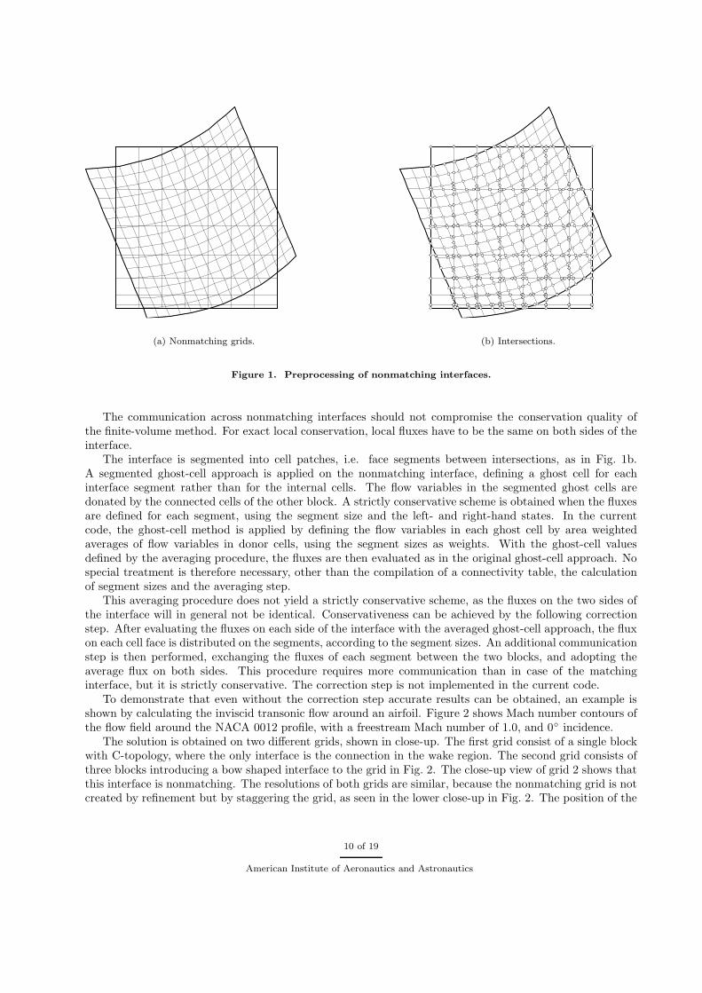
(a) Nonmatching grids. (b) Intersections.

Figure 1. Preprocessing of nonmatching interfaces.

The communication across nonmatching interfaces should not compromise the conservation quality ofthe finite-volume method. For exact local conservation, local fluxes have to be the same on both sides of theinterface.

The interface is segmented into cell patches, i.e. face segments between intersections, as in Fig. 1b.A segmented ghost-cell approach is applied on the nonmatching interface, defining a ghost cell for eachinterface segment rather than for the internal cells. The flow variables in the segmented ghost cells aredonated by the connected cells of the other block. A strictly conservative scheme is obtained when the fluxesare defined for each segment, using the segment size and the left- and right-hand states. In the currentcode, the ghost-cell method is applied by defining the flow variables in each ghost cell by area weightedaverages of flow variables in donor cells, using the segment sizes as weights. With the ghost-cell valuesdefined by the averaging procedure, the fluxes are then evaluated as in the original ghost-cell approach. Nospecial treatment is therefore necessary, other than the compilation of a connectivity table, the calculationof segment sizes and the averaging step.

This averaging procedure does not yield a strictly conservative scheme, as the fluxes on the two sides ofthe interface will in general not be identical. Conservativeness can be achieved by the following correctionstep. After evaluating the fluxes on each side of the interface with the averaged ghost-cell approach, the fluxon each cell face is distributed on the segments, according to the segment sizes. An additional communicationstep is then performed, exchanging the fluxes of each segment between the two blocks, and adopting theaverage flux on both sides. This procedure requires more communication than in case of the matchinginterface, but it is strictly conservative. The correction step is not implemented in the current code.

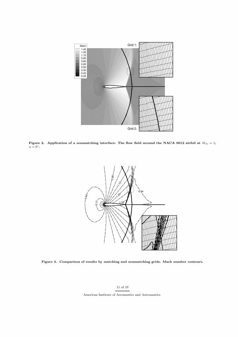
To demonstrate that even without the correction step accurate results can be obtained, an example isshown by calculating the inviscid transonic flow around an airfoil. Figure 2 shows Mach number contours ofthe flow field around the NACA 0012 profile, with a freestream Mach number of 1.0, and 0 incidence.

The solution is obtained on two different grids, shown in close-up. The first grid consist of a single blockwith C-topology, where the only interface is the connection in the wake region. The second grid consists ofthree blocks introducing a bow shaped interface to the grid in Fig. 2. The close-up view of grid 2 shows thatthis interface is nonmatching. The resolutions of both grids are similar, because the nonmatching grid is notcreated by refinement but by staggering the grid, as seen in the lower close-up in Fig. 2. The position of the

10 of 19


Mach1.401.251.100.950.800.650.500.350.200.05

Grid 2:

Grid 1:

Figure 2. Application of a nonmatching interface: The flow field around the NACA 0012 airfoil at M∞ = 1,α = 0.

0.84

0.77

0.98

1.12

1.25

1.39

0.84

Figure 3. Comparison of results by matching and nonmatching grids. Mach number contours.

11 of 19


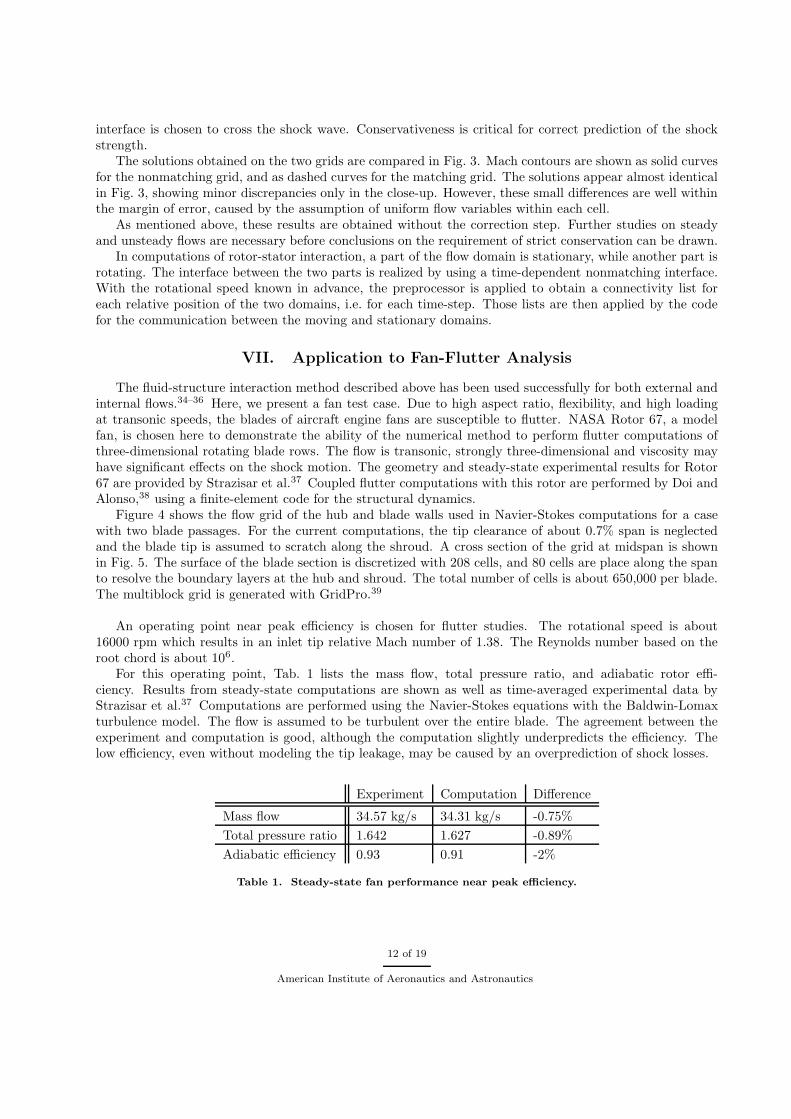
interface is chosen to cross the shock wave. Conservativeness is critical for correct prediction of the shockstrength.

The solutions obtained on the two grids are compared in Fig. 3. Mach contours are shown as solid curvesfor the nonmatching grid, and as dashed curves for the matching grid. The solutions appear almost identicalin Fig. 3, showing minor discrepancies only in the close-up. However, these small differences are well withinthe margin of error, caused by the assumption of uniform flow variables within each cell.

As mentioned above, these results are obtained without the correction step. Further studies on steadyand unsteady flows are necessary before conclusions on the requirement of strict conservation can be drawn.

In computations of rotor-stator interaction, a part of the flow domain is stationary, while another part isrotating. The interface between the two parts is realized by using a time-dependent nonmatching interface.With the rotational speed known in advance, the preprocessor is applied to obtain a connectivity list foreach relative position of the two domains, i.e. for each time-step. Those lists are then applied by the codefor the communication between the moving and stationary domains.

VII. Application to Fan-Flutter Analysis

The fluid-structure interaction method described above has been used successfully for both external andinternal flows.34–36 Here, we present a fan test case. Due to high aspect ratio, flexibility, and high loadingat transonic speeds, the blades of aircraft engine fans are susceptible to flutter. NASA Rotor 67, a modelfan, is chosen here to demonstrate the ability of the numerical method to perform flutter computations ofthree-dimensional rotating blade rows. The flow is transonic, strongly three-dimensional and viscosity mayhave significant effects on the shock motion. The geometry and steady-state experimental results for Rotor67 are provided by Strazisar et al.37 Coupled flutter computations with this rotor are performed by Doi andAlonso,38 using a finite-element code for the structural dynamics.

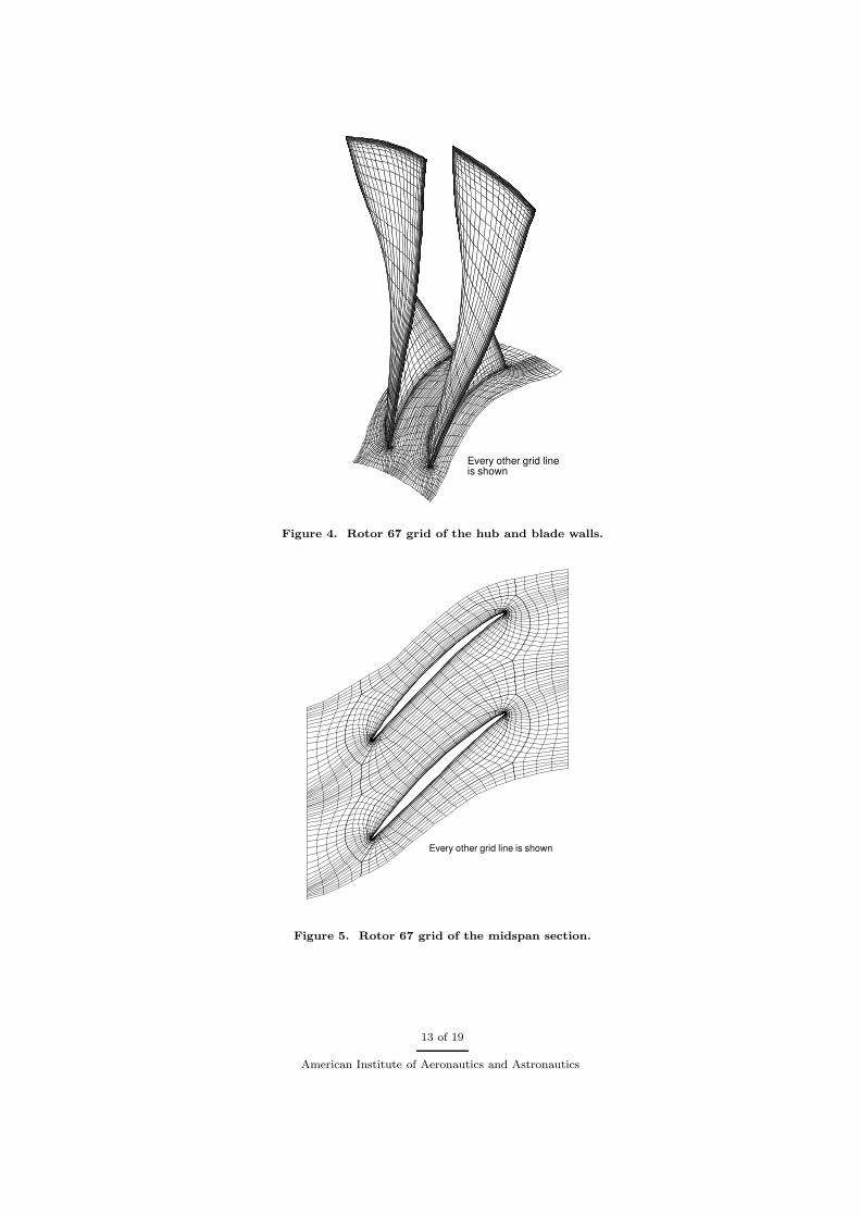
Figure 4 shows the flow grid of the hub and blade walls used in Navier-Stokes computations for a casewith two blade passages. For the current computations, the tip clearance of about 0.7% span is neglectedand the blade tip is assumed to scratch along the shroud. A cross section of the grid at midspan is shownin Fig. 5. The surface of the blade section is discretized with 208 cells, and 80 cells are place along the spanto resolve the boundary layers at the hub and shroud. The total number of cells is about 650,000 per blade.The multiblock grid is generated with GridPro.39

An operating point near peak efficiency is chosen for flutter studies. The rotational speed is about16000 rpm which results in an inlet tip relative Mach number of 1.38. The Reynolds number based on theroot chord is about 106.

For this operating point, Tab. 1 lists the mass flow, total pressure ratio, and adiabatic rotor effi-ciency. Results from steady-state computations are shown as well as time-averaged experimental data byStrazisar et al.37 Computations are performed using the Navier-Stokes equations with the Baldwin-Lomaxturbulence model. The flow is assumed to be turbulent over the entire blade. The agreement between theexperiment and computation is good, although the computation slightly underpredicts the efficiency. Thelow efficiency, even without modeling the tip leakage, may be caused by an overprediction of shock losses.

Experiment Computation Difference

Mass flow 34.57 kg/s 34.31 kg/s -0.75%

Total pressure ratio 1.642 1.627 -0.89%

Adiabatic efficiency 0.93 0.91 -2%

Table 1. Steady-state fan performance near peak efficiency.

12 of 19


Every other grid lineis shown

Figure 4. Rotor 67 grid of the hub and blade walls.

Every other grid line is shown

Figure 5. Rotor 67 grid of the midspan section.

13 of 19


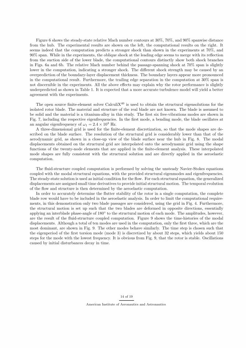
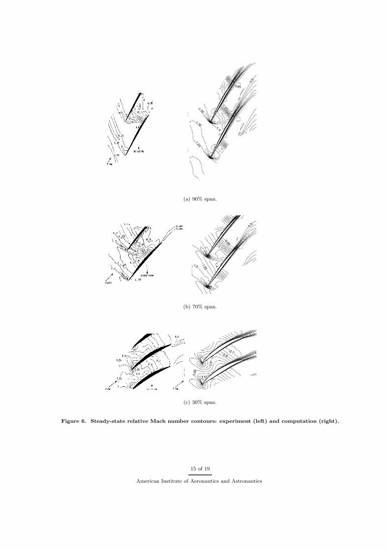
Figure 6 shows the steady-state relative Mach number contours at 30%, 70%, and 90% spanwise distancefrom the hub. The experimental results are shown on the left, the computational results on the right. Itseems indeed that the computation predicts a stronger shock than shown in the experiments at 70%, and90% span. While in the experiments, the oblique shock at the leading edge seems to merge with its reflectionfrom the suction side of the lower blade, the computational contours distinctly show both shock branchesin Figs. 6a and 6b. The relative Mach number behind the passage-spanning shock at 70% span is slightlylower in the computation, indicating a stronger shock. The different shock strength may be caused by anoverprediction of the boundary-layer displacement thickness. The boundary layers appear more pronouncedin the computational result. Furthermore, the trailing edge separation in the computation at 30% span isnot discernible in the experiments. All the above effects may explain why the rotor performance is slightlyunderpredicted as shown in Table 1. It is expected that a more accurate turbulence model will yield a betteragreement with the experiments.

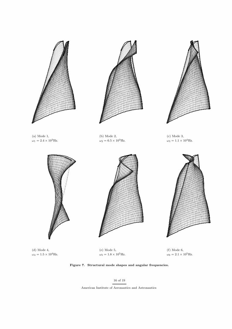
The open source finite-element solver CalculiX40 is used to obtain the structural eigensolutions for theisolated rotor blade. The material and structure of the real blade are not known. The blade is assumed tobe solid and the material is a titanium-alloy in this study. The first six free-vibrations modes are shown inFig. 7, including the respective eigenfrequencies. In the first mode, a bending mode, the blade oscillates atan angular eigenfrequency of ω1 = 2.4 × 103 Hz.

A three-dimensional grid is used for the finite-element discretization, so that the mode shapes are de-scribed on the blade surface. The resolution of the structural grid is considerably lower than that of theaerodynamic grid, as shown in a close-up view of the blade surface near the hub in Fig. 8. The modaldisplacements obtained on the structural grid are interpolated onto the aerodynamic grid using the shapefunctions of the twenty-node elements that are applied in the finite-element analysis. These interpolatedmode shapes are fully consistent with the structural solution and are directly applied in the aeroelasticcomputation.

The fluid-structure coupled computation is performed by solving the unsteady Navier-Stokes equationscoupled with the modal structural equations, with the provided structural eigenmodes and eigenfrequencies.The steady-state solution is used as initial condition for the flow. For each structural equation, the generalizeddisplacements are assigned small time derivatives to provide initial structural motion. The temporal evolutionof the flow and structure is then determined by the aeroelastic computation.

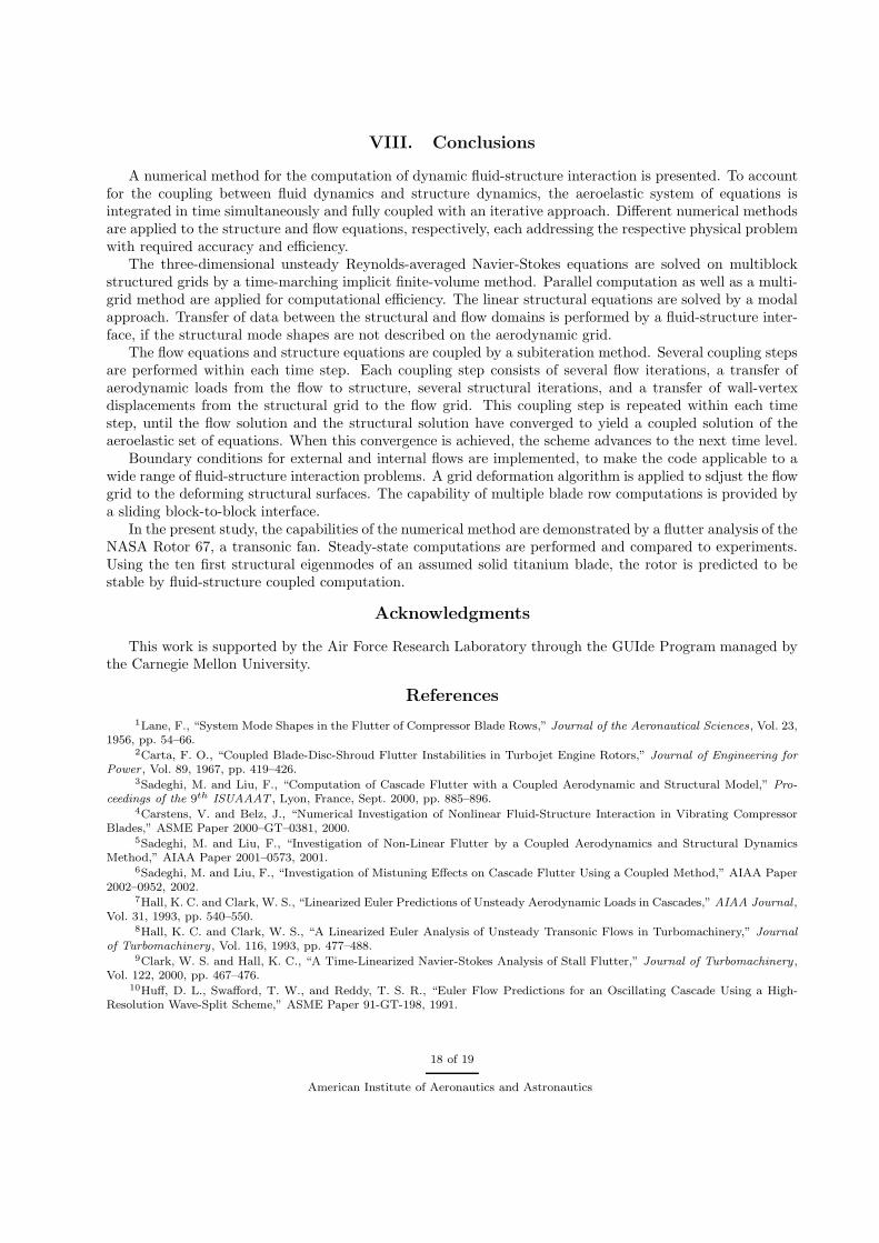
In order to accurately determine the flutter stability of the rotor in a single computation, the completeblade row would have to be included in the aeroelastic analysis. In order to limit the computational require-ments, in this demonstration only two blade passages are considered, using the grid in Fig. 4. Furthermore,the structural motion is set up such that the two blades are deformed in opposite directions, essentiallyapplying an interblade phase-angle of 180 to the structural motion of each mode. The amplitudes, however,are the result of the fluid-structure coupled computation. Figure 9 shows the time-histories of the modaldisplacements. Although a total of ten modes are used in the computation, only the first three, which are themost dominant, are shown in Fig. 9. The other modes behave similarly. The time step is chosen such thatthe eigenperiod of the first torsion mode (mode 3) is discretized by about 32 steps, which yields about 150steps for the mode with the lowest frequency. It is obvious from Fig. 9, that the rotor is stable. Oscillationscaused by initial disturbances decay in time.

14 of 19


(a) 90% span.

(b) 70% span.

(c) 30% span.

Figure 6. Steady-state relative Mach number contours: experiment (left) and computation (right).

15 of 19


(a) Mode 1,

ω1 = 2.4 × 103Hz.

(b) Mode 2,

ω2 = 6.5 × 103Hz.

(c) Mode 3,

ω3 = 1.1 × 104Hz.

(d) Mode 4,

ω4 = 1.5 × 104Hz.

(e) Mode 5,

ω5 = 1.8 × 105Hz.

(f) Mode 6,

ω6 = 2.1 × 105Hz.

Figure 7. Structural mode shapes and angular frequencies.

16 of 19


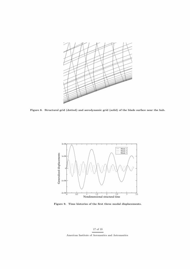
Figure 8. Structural grid (dotted) and aerodynamic grid (solid) of the blade surface near the hub.

0 0.5 1 1.5 2 2.5 3 3.5Nondimensional structural time

-2e-06

-1e-06

0

1e-06

2e-06

Gen

eral

ized

dis

plac

emen

ts

Mode 1Mode 2Mode 3

Figure 9. Time histories of the first three modal displacements.

17 of 19


VIII. Conclusions

A numerical method for the computation of dynamic fluid-structure interaction is presented. To accountfor the coupling between fluid dynamics and structure dynamics, the aeroelastic system of equations isintegrated in time simultaneously and fully coupled with an iterative approach. Different numerical methodsare applied to the structure and flow equations, respectively, each addressing the respective physical problemwith required accuracy and efficiency.

The three-dimensional unsteady Reynolds-averaged Navier-Stokes equations are solved on multiblockstructured grids by a time-marching implicit finite-volume method. Parallel computation as well as a multi-grid method are applied for computational efficiency. The linear structural equations are solved by a modalapproach. Transfer of data between the structural and flow domains is performed by a fluid-structure inter-face, if the structural mode shapes are not described on the aerodynamic grid.

The flow equations and structure equations are coupled by a subiteration method. Several coupling stepsare performed within each time step. Each coupling step consists of several flow iterations, a transfer ofaerodynamic loads from the flow to structure, several structural iterations, and a transfer of wall-vertexdisplacements from the structural grid to the flow grid. This coupling step is repeated within each timestep, until the flow solution and the structural solution have converged to yield a coupled solution of theaeroelastic set of equations. When this convergence is achieved, the scheme advances to the next time level.

Boundary conditions for external and internal flows are implemented, to make the code applicable to awide range of fluid-structure interaction problems. A grid deformation algorithm is applied to sdjust the flowgrid to the deforming structural surfaces. The capability of multiple blade row computations is provided bya sliding block-to-block interface.

In the present study, the capabilities of the numerical method are demonstrated by a flutter analysis of theNASA Rotor 67, a transonic fan. Steady-state computations are performed and compared to experiments.Using the ten first structural eigenmodes of an assumed solid titanium blade, the rotor is predicted to bestable by fluid-structure coupled computation.

Acknowledgments

This work is supported by the Air Force Research Laboratory through the GUIde Program managed bythe Carnegie Mellon University.

References

1Lane, F., “System Mode Shapes in the Flutter of Compressor Blade Rows,” Journal of the Aeronautical Sciences, Vol. 23,1956, pp. 54–66.

2Carta, F. O., “Coupled Blade-Disc-Shroud Flutter Instabilities in Turbojet Engine Rotors,” Journal of Engineering forPower , Vol. 89, 1967, pp. 419–426.

3Sadeghi, M. and Liu, F., “Computation of Cascade Flutter with a Coupled Aerodynamic and Structural Model,” Pro-ceedings of the 9th ISUAAAT , Lyon, France, Sept. 2000, pp. 885–896.

4Carstens, V. and Belz, J., “Numerical Investigation of Nonlinear Fluid-Structure Interaction in Vibrating CompressorBlades,” ASME Paper 2000–GT–0381, 2000.

5Sadeghi, M. and Liu, F., “Investigation of Non-Linear Flutter by a Coupled Aerodynamics and Structural DynamicsMethod,” AIAA Paper 2001–0573, 2001.

6Sadeghi, M. and Liu, F., “Investigation of Mistuning Effects on Cascade Flutter Using a Coupled Method,” AIAA Paper2002–0952, 2002.

7Hall, K. C. and Clark, W. S., “Linearized Euler Predictions of Unsteady Aerodynamic Loads in Cascades,” AIAA Journal ,Vol. 31, 1993, pp. 540–550.

8Hall, K. C. and Clark, W. S., “A Linearized Euler Analysis of Unsteady Transonic Flows in Turbomachinery,” Journalof Turbomachinery , Vol. 116, 1993, pp. 477–488.

9Clark, W. S. and Hall, K. C., “A Time-Linearized Navier-Stokes Analysis of Stall Flutter,” Journal of Turbomachinery ,Vol. 122, 2000, pp. 467–476.

10Huff, D. L., Swafford, T. W., and Reddy, T. S. R., “Euler Flow Predictions for an Oscillating Cascade Using a High-Resolution Wave-Split Scheme,” ASME Paper 91-GT-198, 1991.

18 of 19


11Moffatt, S. and He, L., “Blade Forced Response Predictions for Industrial Gas Turbines, Part I: Methodologies,” ASMEPaper GT2003–38640, 2003.

12Hall, K. C., Florea, R., and Lanzkron, P. J., “A Reduced Order Model of Unsteady Flows in Turbomachinery,” Journalof Turbomachinery , Vol. 117, 1995.

13Epureanu, B. I., Dowell, E. H., and Hall, K. C., “Reduced Order Models of Unsteady Transonic Flows in Turbomachinery,”Journal of Fluids and Structures, Vol. 14, 2000, pp. 1215–1234.

14Sisto, F., Thangam, S., and Abdel-Rahim, A., “Computational Prediction of Stall Flutter in Cascaded Airfoils,” AIAAJournal , Vol. 29, 1991, pp. 1161–1167.

15Abdel-Rahim, A., Sisto, F., and Thangam, S., “Computational Study of Stall Flutter in Cascaded Airfoils,” Journal ofTurbomachinery , Vol. 115, 1993, pp. 157–166.

16Bakhle, M. A., Reddy, T. S. R., and Jr., T. G. K., “Time Domain Flutter Analysis of Cascades Using a Full-PotentialSolver,” AIAA Journal , Vol. 30, 1992, pp. 163–170.

17Sayma, A. I., Vahdati, M., and Imregun, M., “An Integrated Nonlinear Approach for Turbomachinery Forced ResponsePrediction – Part I: Formulation,” Journal of Fluids and Structures, Vol. 14, 2000, pp. 87–101.

18Sayma, A. I., Vahdati, M., and Imregun, M., “An Integrated Nonlinear Approach for Turbomachinery Forced ResponsePrediction – Part II: Case Studies,” Journal of Fluids and Structures, Vol. 14, 2000, pp. 87–101.

19Breard, C., Imregun, M., Sayma, A., and Vahdati, M., “Flutter Stability Analysis of a Complete Fan Assembly,” AIAApaper 99-0238, 1999.

20Jameson, A., “Time Dependent Calculations Using Multigrid, with Applications to Unsteady Flows Past Airfoils andWings,” AIAA Paper 81–1259, 1991.

21Wilcox, D. C., “Reassessment of the Scale-Determining Equation for Advanced Turbulence Models,” AIAA Journal ,Vol. 26, 1988, pp. 1299–1310.

22Liu, F. and Zheng, X., “A Strongly-Coupled Time-Marching Method for Solving the Navier-Stokes and k-ω TurbulenceModel Equations with Multigrid,” Journal of Computational Physics, Vol. 128, 1996, pp. 289–300.

23Liu, F. and Ji, S., “Unsteady Flow Calculations with a Multigrid Navier-Stokes Method,” AIAA Journal , Vol. 34, No. 10,Oct. 1996, pp. 2047–2053.

24Jameson, A., Schmidt, W., and Turkel, E., “Numerical Solutions of the Euler Equations by Finite Volume Methods UsingRunge-Kutta Time-Stepping Schemes,” AIAA Paper 81–1259, 1981.

25Jameson, A., “Analysis and Design of Numerical Schemes for Gas Dynamics 1: Artificial Diffusion, Upwind Biasing,Limiters and Their Effect on Accuracy and Multigrid Convergence,” Int’l Journal of Computational Fluid Dynamics, Vol. 4,1995, pp. 171–218.

26Jameson, A., “Analysis and Design of Numerical Schemes for Gas Dynamics 2: Artificial Diffusion and Discrete ShockStructure,” Int’l Journal of Computational Fluid Dynamics, Vol. 5, 1995, pp. 1–38.

27Saxer, A. P., A Numerical Analysis of 3-D Inviscid Stator/Rotor Interactions Using Non-Reflecting Boundary Condi-tions, Ph.D. thesis, Massachusetts Institute of Technology, 1992.

28Giles, M. B., “Non-Reflecting Boundary Conditions for the Unsteady Euler Equations,” Technical Report CFDL-TR-88-1,Massachusetts Institute of Technology, 1988.

29Giles, M. B., “UNSFLO: A Numerical Method for the Calculation of Unsteady Flow in Turbomachinery,” GTL ReportNo. 205, Massachusetts Institute of Technology, Gas Turbine Lab, 1988.

30Goura, G. S. L., Badcock, K. J., Woodgate, M. A., and Richards, B. E., “Transformation Methods for the Time MarchingAnalysis of Flutter,” AIAA Paper 2001–2457, 2001.

31Chen, H. H., Chang, K. C., Tzong, T., and Cebeci, T., “Aeroelastic Analysis of Wing and Wing/Fuselage Configurations,”AIAA Paper 98–0907, 1998.

32Sadeghi, M., Liu, F., Lai, K. L., and Tsai, H. M., “Application of Three-Dimensional Interfaces for Data Transfer inAeroelastic Computations,” AIAA Paper 2004-5376, 2004.

33Wong, A. S. F., Tsai, H. M., Zhu, Y., Cai, J., and Liu, F., “Unsteady Flow Calculation with a Multi-Block Moving MeshAlgorithm,” AIAA Paper 2000–1002, 2000.

34Liu, F., Cai, J., Zhu, Y., Tsai, H. M., and Wong, A. S. F., “Calculation of Wing Flutter by a Coupled Fluid-StructureMethod,” Journal of Aircraft , Vol. 38, 2001, pp. 334–342.

35Sadeghi, M., Yang, S., Liu, F., and Tsai, H. M., “Parallel Computation of Wing Flutter with a Coupled Navier-Stokes/CSD Method,” AIAA Paper 2003-1347, 2003.

36Sadeghi, M., Yang, S., and Liu, F., “Computation of Uncoupled and Coupled Aeroelasticity of Three-Dimensional BladeRows,” AIAA Paper 2004-0192, 2004.

37Strazisar, A. J., Wood, J. R., Hathaway, M. D., and Suder, K. L., “Laser Anemometer Measurements in a TransonicAxial-Flow Fan Rotor,” NASA TP 2879, Nov. 1989.

38Doi, H. and Alonso, J. J., “Fluid/Structure Coupled Aeroelastic Computations for Transonic Flows in Turbomachinery,”ASME Paper 2002–GT–30313, 2002.

39Program Development Corporation, “GridPro v4.2 User’s Guide and Reference Manual,” Tech. rep., 1999.40Dhondt, G., “CalculiX CrunchiX User’s Manual Version 1.2,” Tech. rep., 2004.

19 of 19


Documents

Coupled Fluid-Structure Simulation for Turbomachinery ...fliu.eng.uci.edu/Publications/C061.pdf · Coupled Fluid-Structure Simulation for Turbomachinery Blade Rows ... study of other