Counting and Measuring Ultrastructural Features of ...cshprotocols.cshlp.org/content/2013/7/pdb.top071886.full.pdf · Counting and Measuring Ultrastructural Features of Biological

Topic Introduction

Counting and Measuring Ultrastructural Featuresof Biological Samples

Mark J. West

Ultrastructural features of cells can be fractions of a micrometer in diameter, and electron microscopyis needed to resolve them to a degree that is compatible with stereological techniques. Because the focaldepth of transmission electron microscopy (TEM) images is thousands of times greater than thethickness of the sections used with TEM, virtual sectioning of sections suitable for TEM is not possible,as it is with light microscopy and the optical disector probe.With features the size of neuronal synapses,for example, this necessitates the use of physical sections and physical disectors. Regardless of how theimaging is performed, the design of stereological studies for quantifying ultrastructural features will beessentially the same as that used in the example described here, which uses physically separatedultrathin sections viewed with conventional TEM to estimate the number and size of synapses in aparticular brain region.

EXAMPLE INVOLVING ESTIMATION OF NUMBER AND SIZE OF SYNAPSES

The stereological method described here for estimating the total number of synaptic contactsNSYN in awell-defined region of the brain is based on a two-step procedure. This approach has been shown to beapplicable to regions of the nervous system that vary significantly in absolute volume (Geinisman et al.1996; Scheff et al. 2007; West et al. 2009). The total number of synapses NSYN can be estimated as theproduct of an estimate of the volume of the region of interest or reference volume VREF made by pointcounting and an estimate of the numerical density of synapses made NVSYN with physical disectors:

NSYN = VREF × NVSYN . (1)

PREPARATION OF TISSUE

Standard fixation and staining methods used in conventional electron microscopy of the nervoussystem can be used for the stereological analysis of synapses.

In the example presented here, VREF is the stratum radiatum of CA1 of the hippocampus, that is,srCA1, of the C57Bl/6 mouse. The tissue was prepared according to traditional electron micrograph(EM) protocols. Subsequently, lead citrate was used to stain ultrathin sections of tissue after embed-ding in Epon. This tissue proved to be suitable for the identification of synaptic contact specializa-tions. Selective staining of the paramembranous specializations with ethanolic phosphotungstic acid(EPTA) can be used under special circumstances and with some caveats. EPTA has been used inhuman postmortem material to stain synaptic contacts (Tang et al. 2001), which are apparently more

Adapted from Basic Stereology for Biologists and Neuroscientists by Mark J. West. CSHL Press, Cold Spring Harbor, NY, USA, 2012.

© 2013 Cold Spring Harbor Laboratory PressCite this article as Cold Spring Harb Protoc; 2013; doi:10.1101/pdb.top071886

593

Cold Spring Harbor Laboratory Press on June 24, 2018 - Published by http://cshprotocols.cshlp.org/Downloaded from

http://cshprotocols.cshlp.org/

http://www.cshlpress.com

robust than the membranes of cells and organelles. However, the lack of membrane features in thesepreparations makes it difficult to differentiate between segmented and nonsegmented postsynapticdensities (PSDs), and between synaptic contacts and other cellular organelles such as mitochondria,spine apparati, and lysosomes that stain in EPTA-stained tissue.

SAMPLING THE TISSUE

Estimating VREF

Preparing a Systematic Series of Sections for Estimating VREF

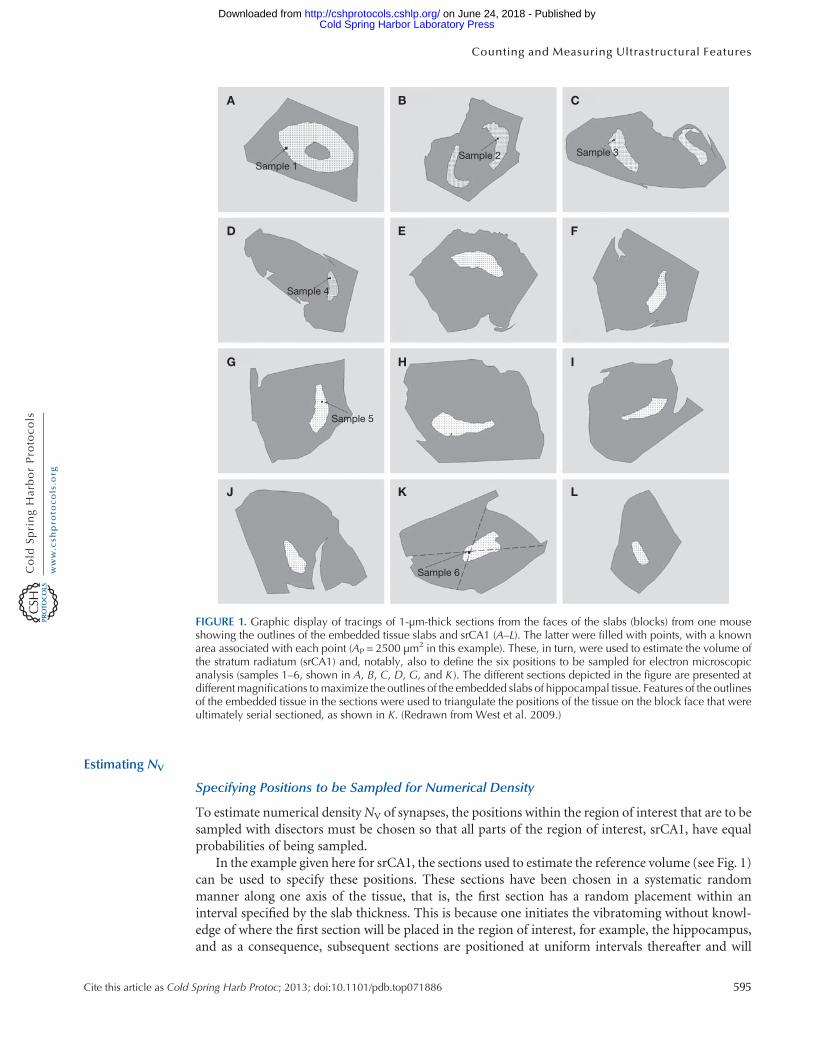
The first phase of the sampling involves preparing the material so that an unbiased estimate can bemade of a brain region from a series of parallel sections through the entire region of interest, VREF.As pointed out in Estimating Volume in Biological Structures (West 2012a), an unbiased estimate ofthe volume of a region of interest can be obtained using point-counting techniques and Cavalieri’sprinciple. Regardless of the size of the region of interest (the hippocampus of an elephant or a mouse),12–18 equally spaced sections will be needed to make the estimate of the reference volume. (Therationale for considering this number of sections to be optimal is described in The Precision ofEstimates in Stereological Analyses [West 2012b] andOptimizing the Sampling Scheme for a Stereo-logical Study: HowMany Individuals, Sections and Probes Should Be Used [West 2013a].) In the caseof the example provided here, for the mouse srCA1, this was accomplished by cutting the entire braininto 300-μm-thick slabs with a vibratome, staining and embedding the portions of the slabs thatcontained hippocampus, and cutting one semithin 1- to 2-μm-thick section from the correspondingsurfaces of each of the slabs. This resulted in 12–14 equally spaced sections throughout the entireregion of interest. The maximum thickness of the slabs should not exceed 1 mm to ensure that thetissue can be thoroughly osmicated, block stained, and infiltrated with embeddingmedium. Figure 1 isa depiction of a series of parallel sections through the hippocampus fromone side of amouse brain thatwere used to estimate the volume of srCA1, VsrCA1.

As pointed out in The Precision of Estimates in Stereological Analyses (West 2012b), Systematicversus Random Sampling in Stereological Studies (West 2012c), Getting Started in Stereology (West2013b), and Optimizing the Sampling Scheme for a Stereological Study: How Many Individuals,Sections and Probes Should Be Used (West 2013a), one usually does not needmore than 150 points inall to estimate the volume of regions with complex shapes, if one has between 12 and 18 sections.However, in this example, a very large number of points was used to facilitate the process of definingthe positions to be sampled for NV, as described in the section Relationship Equations for S and L areTissue Orientation Sensitive in Isotropy, iSectors, and Vertical Sections in Stereology (West 2013c).This is relatively easy to achieve with the “autofill” feature of stereology software packages.

VsrCA1 = SPsrCA1 × AP × T. (2)

Delineation of Region of Interest is Critical

Delineation of the region of interest is critical for the estimation of the total number of synapses and isthe most likely source of discrepancies in stereological studies performed by different investigators.The statistical significance of differences in total number of synapses in any one study can also beaffected by small variations in the delineation process. It is therefore important that rigorous defini-tions of the borders be established a priori and reported in detail. In the example used here, srCA1,the borders with the subiculum and molecular layer are particularly subject to investigator variabil-ity (Fig. 2) (West et al. 2009). It is also important that the preparation and analysis of the tissuebe performed without investigator knowledge of the group identity of the mice, so that any vari-ability in the delineation process contributes equally to the variances of estimates used for comparativepurposes.

594 Cite this article as Cold Spring Harb Protoc; 2013; doi:10.1101/pdb.top071886

M.J. West




Estimating NV

Specifying Positions to be Sampled for Numerical Density

To estimate numerical densityNV of synapses, the positions within the region of interest that are to besampled with disectors must be chosen so that all parts of the region of interest, srCA1, have equalprobabilities of being sampled.

In the example given here for srCA1, the sections used to estimate the reference volume (see Fig. 1)can be used to specify these positions. These sections have been chosen in a systematic randommanner along one axis of the tissue, that is, the first section has a random placement within aninterval specified by the slab thickness. This is because one initiates the vibratoming without knowl-edge of where the first section will be placed in the region of interest, for example, the hippocampus,and as a consequence, subsequent sections are positioned at uniform intervals thereafter and will

A B C

D E F

G H I

J K L

Sample 6

Sample 5

Sample 4

Sample 1Sample 2 Sample 3

FIGURE 1. Graphic display of tracings of 1-µm-thick sections from the faces of the slabs (blocks) from one mouseshowing the outlines of the embedded tissue slabs and srCA1 (A–L). The latter were filled with points, with a knownarea associated with each point (AP = 2500 µm2 in this example). These, in turn, were used to estimate the volume ofthe stratum radiatum (srCA1) and, notably, also to define the six positions to be sampled for electron microscopicanalysis (samples 1–6, shown in A, B, C, D, G, and K ). The different sections depicted in the figure are presented atdifferent magnifications tomaximize the outlines of the embedded slabs of hippocampal tissue. Features of the outlinesof the embedded tissue in the sections were used to triangulate the positions of the tissue on the block face that wereultimately serial sectioned, as shown in K. (Redrawn from West et al. 2009.)

Cite this article as Cold Spring Harb Protoc; 2013; doi:10.1101/pdb.top071886 595

Counting and Measuring Ultrastructural Features




constitute a systematic random series of sections. Sections chosen in this manner have an equalprobability of containing any synapse in srCA1. Because of the very large number of synapses thatcan be expected to be in any one slab, it is necessary to limit the next step in the sampling, that is, withdisectors, to small regions of the slabs. These subsamples must be positioned so that all parts of thesurface of the slabs (all synapses at that level) have equal probability of being sampled. They arepositioned at a systematic random set of positions within the x,y dimensions of the surface of the slabs.As a consequence, the amount of sampling performed on any one slab is proportional to the area ofthe cut surface of the slab. This can be done with the aid of the point-counting grid used to estimateVREF, as shown in Figure 1.

In the example presented here for srCA1, six systematic random positions within the threedimensions of the region of interest were sampled to obtain estimates of NV. A more detailed dis-cussion follows regarding the amount of positions as well as the reasons why six positions should besampled in this example. First, a method for physically specifying the actual positions of any numberof samples is considered. The sum of the areas of the profiles of the region of interest on the semithinsections used to estimate VREF (see above) corresponds to the total area of the sections to be sampled.Dividing this area by the number of samples one wishes to position within the three dimensions (inthis example, six) results in an area that corresponds to the distance, in two dimensions, between thepositions to be sampled on the sections. A similar process is described for the spacing of 150 opticaldisector samples in Getting Started in Stereology (West 2013b). (For more information on opticaldisectors, see the section entitled The Optical Disector Probe in Estimating Object Number inBiological Structures [West 2012d].) Because each point used in the point-counting grid has aknown area associated with it (Fig. 1), the area of the profile of the region of interest, srCA1, canalso be expressed by the number of points that will hit the profile. The area between samples isequivalent to a set number of points. After a random start within the first interval of this numberof points, the points at intervals of this number can be defined subsequently (Table 1). The positionsof these points can be viewed on images of the semithin sections used for point counting (Fig. 1).Graphic representations of the superimposed tracings of the outlines of the edges of the slab ofembedded tissue, boundaries of the region of interest, and representations of the point-countinggrid can then be used to identify the positions in the sections to be sampled. Using features at theedge of the slab and the position of the sample (a point), corresponding positions on the surface of theblock face can be defined, by triangulation, and small regions of the block face at those positionstrimmed down for serial ultramicrotomy.

FIGURE 2. Semithin transverse Epon section throughthe hippocampus of a transgenic mouse stained withToluidine Blue showing srCA1 marked by a blackpoint-counting grid. Critical borders are indicated byarrows. Scale bar, 500 µm. (Redrawn from West et al.2009.)


M.J. West




Number of Stacks Needed

Returning to the issue of how many sites should be sampled with physical disectors to obtain anestimate of NV, it should be pointed out once again that there is no set a priori rule. In general, theanswer can only be derived after a pilot analysis of the sources of variance that contribute to theparameter that is ultimately used in the comparisons, for example, of group means. (For more detailsregarding this process, see Optimizing the Sampling Scheme for a Stereological Study: How ManyIndividuals, Sections and Probes Should Be Used [West 2013a].) The primary factor affecting thevariability in the samples of NV is the homogeneity of the distribution of synapses in the region ofinterest. If the numerical density is the same in all parts of the region of interest, one sample of 100–200 neurons should suffice. However, because we do not want to assume anything regarding orga-nization of the structures, such as the absence of gradients in the numerical density of synapses alongthe three axes of the region of interest, at least two (random) samples are required to develop somefeeling for the variability in the estimate ofNV. In an earlier study of synapse number based on similarprinciples (Geinisman et al. 1996), six samples were shown to capture enough of the variability innumerical density that the variance of the final estimator of total number (which is the sum of thevariances of the estimatesNV andVREF) was sufficient for comparative studies (Geinisman et al. 2004).In the original study, the use of six samples was considered to be a reasonable balance betweenvariability in synapse density that might be expected from site to site and the amount of worknecessary to make each individual sample of numerical density at a site, that is, cut, image, andanalyze a stack of physical densities. Again, the appropriateness of using six samples can only beconfirmed after comparisons of parameters at higher levels of the sampling scheme, such as groupmeans. (See discussion of analysis of variance inOptimizing the Sampling Scheme for a StereologicalStudy: How Many Individuals, Sections and Probes Should Be Used [West 2013a].) In the exampleused here, this turned out to be the case when six samples were used to estimate the NV in eachindividual, in that the mean observed relative variance OCE

2of the estimator ofNSYN was less than the

observed relative variance of the group mean (see Eq. 1 in The Precision of Estimates in StereologicalAnalyses [West 2012b]). The estimate of the numerical density in an individual is the mean of a setnumber of samples within that individual. In the example given here, there are six samples of NV ineach individual.

TABLE 1. Portion of a worksheet that contains point-count data from the sections shown in Figure 3

MW: 557

Block (section) Points (P) ΣPStack

position BlockSample 1position

Sample 2position

Sample 3position

Sample 4position

Sample 5position

Sample 6position

1 786 786 424 1 4242 616 1402 946 2 1603 554 1956 1468 3 664 204 2160 1990 4 345 193 2353 56 129 2482 67 112 2594 2512 7 308 142 2736 89 132 2868 910 93 2961 1011 102 3063 3034 11 7312 69 3132 12Interval ΣP/6 522

Data used tomake a systematic random selection of six positions in srCA1 for EM analysis. The total number of points on all sections (3132) isdivided by 6 to determine the interval between the points to be sampled (522). The first position for sampling is the point that has a randomnumber between 1 and 522, that is, 424 in this example. Subsequent positions are defined at points that are at 522-point intervals (i.e., thesecond sampling point will be at 424 + 522 or at point 46, which lies on section 2). Note that with this sampling scheme, not all sections aresampled, but all parts of the srCA1 have an equal probability of being in the sample.






Example of Sampling with Stacks

In the example given here, a serial stack of electron micrographs was collected at each of the sixpositions to be sampled. The magnification of the micrographs and the number of sections werechosen so that, on average, �30 synaptic contacts would be sampled (“counted”). This numberensured that �150 synaptic contacts would be sampled when all six samples were collected (seeThe Precision of Estimates in Stereological Analyses [West 2012b] and Optimizing the SamplingScheme for a Stereological Study: HowMany Individuals, Sections and Probes Should Be Used [West2013a] for why 150 samples is an appropriate starting point). Magnification of the images should bethe lowest at which the objects of interest—in this case, synaptic contacts—can be clearly identified.The lowest magnification at which this can be done was chosen because this results in sampling thelargest area of the sections. The larger the area sampled, the larger the volume of tissue contained in astack of images. The volume of the tissue being sampled is also defined by the number of sections inthe stack and the thickness of the sections.

The primary magnification was 13,500×. Gold section series were collected for analysis. Aftercollection on Formvar slot grids, the ultrathin sections were stained with electron-dense metals.

Defining and Counting Synaptic Contacts

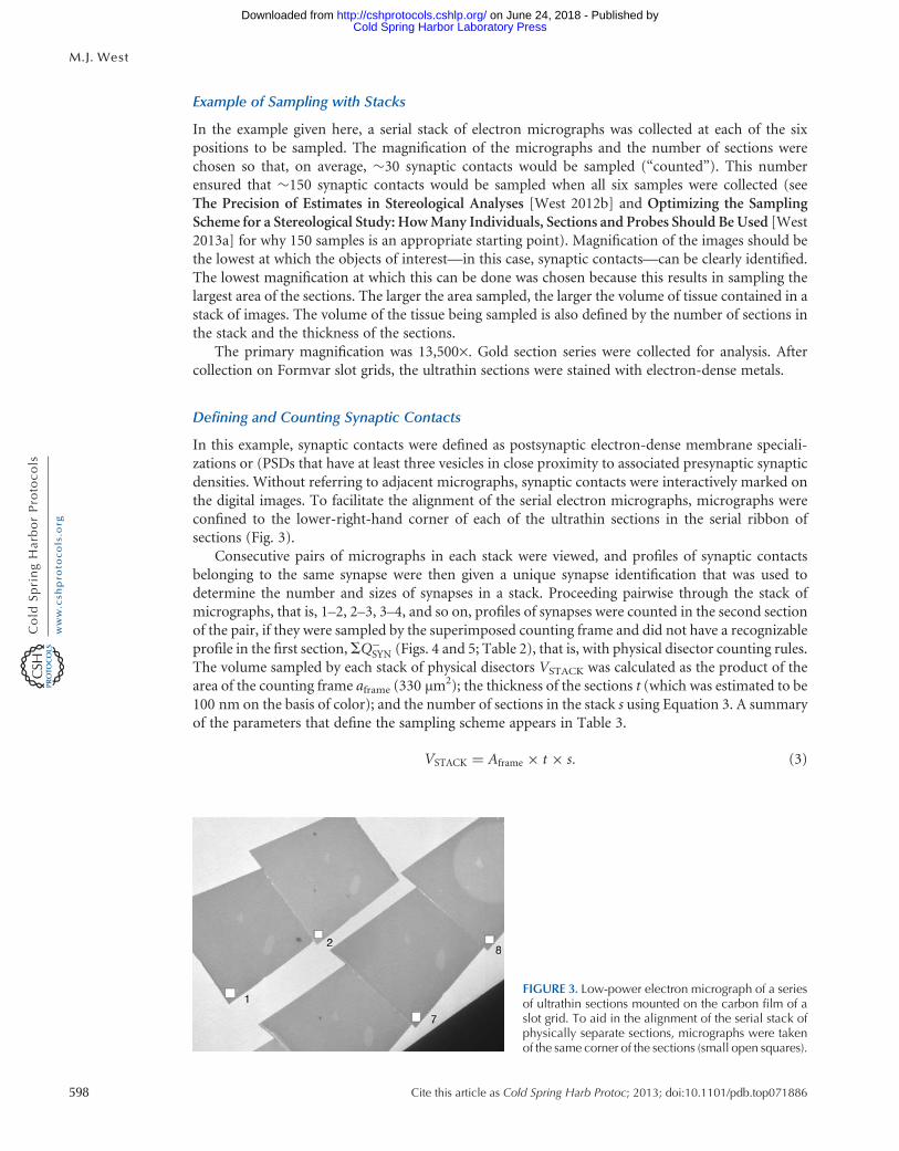
In this example, synaptic contacts were defined as postsynaptic electron-dense membrane speciali-zations or (PSDs that have at least three vesicles in close proximity to associated presynaptic synapticdensities. Without referring to adjacent micrographs, synaptic contacts were interactively marked onthe digital images. To facilitate the alignment of the serial electron micrographs, micrographs wereconfined to the lower-right-hand corner of each of the ultrathin sections in the serial ribbon ofsections (Fig. 3).

Consecutive pairs of micrographs in each stack were viewed, and profiles of synaptic contactsbelonging to the same synapse were then given a unique synapse identification that was used todetermine the number and sizes of synapses in a stack. Proceeding pairwise through the stack ofmicrographs, that is, 1–2, 2–3, 3–4, and so on, profiles of synapses were counted in the second sectionof the pair, if they were sampled by the superimposed counting frame and did not have a recognizableprofile in the first section,SQ−

SYN (Figs. 4 and 5; Table 2), that is, with physical disector counting rules.The volume sampled by each stack of physical disectors VSTACK was calculated as the product of thearea of the counting frame aframe (330 µm

2); the thickness of the sections t (which was estimated to be100 nm on the basis of color); and the number of sections in the stack s using Equation 3. A summaryof the parameters that define the sampling scheme appears in Table 3.

VSTACK = Aframe × t × s. (3)

FIGURE 3. Low-power electron micrograph of a seriesof ultrathin sections mounted on the carbon film of aslot grid. To aid in the alignment of the serial stack ofphysically separate sections, micrographs were takenof the same corner of the sections (small open squares).


M.J. West




In Figure 5, all sectional profiles of synaptic contacts are marked (boxes) on the individual digitalelectron micrographs. Profiles belonging to the same contact are given a unique contact identificationnumber. Contacts that have their first identifiable sectional profile below the first section in the seriesare counted (Table 2), provided that they are sampled by the superimposed unbiased areal countingframe (thin lines around the edge of the micrograph in Fig. 5) (see Estimating Object Number inBiological Structures [West 2012d]). Volume of tissue sampled is calculated as the product of the areaof counting frame Aframe, section thickness t, and number of sections in stack s. The largest length ofthe profiles that belonged to the same synaptic contact is defined as the width of the synaptic contact(Table 1).

There are some caveats that should be mentioned with regard to this measure of synaptic contactsize, because this measure may not be truly unbiased. First, it is assumed that the contact surfaces arerandomly oriented; this was not tested. Second, theremay be synaptic contacts that are not identifiablein the stack because the synaptic cleft lies perfectly in the plane of the section. It has been estimatedthat this can produce an underestimation in total number NSYN by 3% (Tang et al. 2001).

The numerical density of synaptic contacts in each of the six stacks NVSYN(STACK) sampled in anindividual was determined by dividing the number of synapses counted in the stack, SQ−

SYN, by thevolume of the stack VSTACK as shown in the following equation:

NVSYN(STACK) =SQ−

SYN

VSTACK. (4)

The numerical density of synapses in each mouse, NVSYN(MOUSE), is estimated as the mean of the sixsamples of numerical density made in that mouse (Eq. 5). Accordingly, the variance of the estimates ofthe numerical density made in eachmouseNVSYN(MOUSE) is calculated on the basis of a sample size n of six

FIGURE 5. Three serial sections from a larger seriesillustrating counting and measuring procedures per-formed at each sampling site within srCA1 describedin the text. (Redrawn from West et al. 2009.)

FIGURE 4. Consecutive pairs of sections were ana-lyzed while being viewed simultaneously on twocomputer monitors.






independent samples (stacks) of the numerical density:

NVSYN(MOUSE)= mean1−6

SQ−SYN

VSTACK. (5)

Ultrathin Section Thickness t

The thickness at which the ultrathin sections in the stack are cut is determined by two factors. Thesections must be thin enough to be able to identify the objects, and they should be as thick as possibleto maximize the volume of the physical disectors. In the example used here, 100-nm-thick sectionswere chosen with this strategy in mind. Although sections of this thickness do not have the clarity ofthe thinner sections often used in descriptive publications, they do contain more information andthereby require fewer sections to obtain a sample of a certain size.

Numbers of Sections in a Serial Stack

The number of sections in the stack s should be such that the sum of the counts obtained from all ofthe stacks in an individual should be�150. Accordingly, in the example given here, the stack contains�30 synaptic contacts, on average (see Getting Started in Stereology (West 2013b) for an explanationas to why counting �150 synapses is appropriate at the beginning of a study). Because the magnifi-cation has been chosen to be the lowest at which synaptic contacts can be identified, a pilot study

TABLE 2. Stack analysis

Synapse section 1 2 3 4 5 6 7 8 9 10 11 12

1 309 3112 236 289 3123 309 5144 235 427 349 545 4145 218 447 1816 211 2687 2398 4009 719 23410 1069 25511 794 360 264 32912 301

Portion of a worksheet with contact length data showing salient features of the stack analysis. Each filled cell contains a measure of the lengthof a sectional profile of a synaptic contact. Measures of the lengths of the profiles from the same synapse are in the same column. Synapses arecounted if their first recognizable sectional profile in the stack is below the first section of the stack. Accordingly, synapses 1 and 2 are notcounted. Synapse 12 is not included in the width measurements because it is not entirely within the stack.

TABLE 3. Summary of sampling scheme for estimating synapse number and size

AP used to estimate VsrCA1 2500 mm2

T used to estimate VsrCA1 300 µmSections used to estimate VsrCA1 12EM stacks per mouse 6s sections per EM stack 8–14Aframe, EM 3.3 × 108 mm2

t, EM 100 nmSQ−

SYN for estimate of NSYN 210 (146–295)SQ−

SYN for estimate of ASYN 181 (126–247)

(VsrCA1) Volume of stratum radiatum CA1 of hippocampus, (AP) area per point on point grid, (T )distance between corresponding surfaces of slabs used to estimate VsrCA1, (s) sections in a stack, (Aframe)area of disector counting frame, (t) section thickness, (SQ−

SYN) sum of synapses counted in six stacks.


M.J. West




indicated that stacks that were on the order of �10 sections would be adequate to achieve this whensections are 100 nm thick. Although disector stacks with these dimensions can be expected to beapplicable to homologous brain regions in other species, analyses of other brain regions, organelles,and organs require similar pilot studies.

Distance between Sections in the Disector Stack

When sampling structures such as synaptic contacts, which can have diameters <200 nm, it is prudentto record images of immediately adjacent serial sections when generating the stack, lest the smallsynapses go undetected. Theoretically, one can use any distance between the two sections of a disector,provided that the distance is not so great that objects “disappear” between sections. In general, thiscan be ensured if the distance between the sections is half of the smallest dimension of the objects.In the example presented here, every section was used in the stack to avoid missing the smallestsynaptic contacts.

Measuring Section Thickness t

Tomake an estimate of the numerical density, it is necessary to know the volume of the tissue in whichthe objects—synaptic contacts—are counted. The volume of each disector stack is the product of thearea of the section being sampled Aframe, which one can measure on the micrograph when themagnification is known, and the thickness of the stack, which is the number of sections s in thestack, times the average thickness of the sections in the stack�t (Eq. 3). To determine the volume of thedisector stack, one must have information regarding the thickness of the ultrathin sections in thestack. There are several ways to obtain this information, some easier than others. The more rigorousmethods include those based on measurements of cylindrical structures in the tissue (Fiala and Harris2001a) and Small’s fold method based onmeasuring the width of folds in the section (DeGroot 1988).In some cases, it may not be possible to consistently identify the folds or cylindrical structures neededto use these methods.

In the example given here, only series of gold sections were collected for analysis. Sections of thiscolor may range in thickness from 85 to 115 nm (Hayat 1979). As pointed out above, this relativelylarge section thickness was chosen to maximize the volume of physical disectors andmaintain enoughmorphological detail for proper identification of synaptic contacts. Any systematic deviation in thesection thickness from the 100-nm thickness used in the example can be expected to introduce adeviation in the estimates of total synapse number from the true value by a factor that is directlyproportional to the deviation, that is, 15%. This potential bias may account for the slight differences insynapse numerical density in the example provided here as well as those of other investigators, asdiscussed byWest et al. (2009). A technique for counting synapses based on fractionator sampling thateliminates the need for measuring the thickness of ultrathin sections has been described (Witgen et al.2006).

It is important to point out that if the investigators are blind to the identity of the material duringall phases of preparation and analysis and if the tissue is processed and analyzed in random order,variations in section thickness can be expected to be equally distributed in the material and will add tothe variance but not the magnitude of any group differences.

ATROPHY AND TISSUE DEFORMATION

In the example provided here, the calculations used to estimate the total number of synapses takebrain atrophy, postmortem shrinkage, and any shrinkage related to tissue preparation into account.The density of synapses NVSYN—that is, the number per unit volume of tissue estimated with physicaldisectors—is multiplied by the estimate of volume of the region of interest VsrCA1 to calculate the totalsynapse numberNSYN. If the region of interest shrinks or expands during tissue preparation, without achange in the total number of synapses, the numerical density of synapses NVSYN can be expected to






increase or decrease, respectively. However, these changes in numerical density will be accompaniedby a change in the volume of the region VsrCA1 that will directly compensate for the change innumerical density NVSYN, so that the product of the two (NVSYN × VsrCA1) will be the same or thetotal number NSYN will be unchanged.

One can also imagine cases of neuron loss and shrinkage, in which the numerical density remainsthe same, and cases of tissue expansion and neuron loss, in which the numerical density increases. Theimportant feature of the design-based methods used here is that volume changes have no effect on theestimate of total synapse number. Measures of numerical densities by themselves are not adequatedescriptors of global (within a defined region) loss or gain (Nyengaard and Gundersen 2006). Only byrelating the numerical density of synapses to the volume of the structure can one make statementsregarding total number and thereby loss or gain of synapses.

Changes in the dendritic arborization and in other compartments within the tissue will not havean effect on the estimates of synapse number made with the procedure used here. The six samples ofnumerical density in an animal, each of which was composed of eight to 12 serial electron micro-graphs, were placed in a systematic randommanner throughout the region of interest. Samples or partof samples that included distrophic neurites, plaques (see Fig. 2), or other nonneuronal elements, suchas blood vessels, were included. Because the sampling could also include plaques, vessels, and possiblydistrophic dendritic processes, the number of synapses counted in each disector varied considerably.However, when the sampling is designed so that all parts of the region of interest have an equalprobability of being sampled, as was done in the present study, no corrections need be made forplaques, vessels, distrophic dentrites, or vessels, in that they already have been taken into account bybeing included in the samples in correct proportion.

ANALYSIS OF SIZE DISTRIBUTIONS

Information in the disector stacks (Table 2) can be used to evaluate the size of the objects. Number-weighted size distributions, using local estimators or serial reconstructions, can be obtained fromobjects that lie completely within the stack. In these cases, it is therefore of interest to have a stack thathas enough sections so that the largest objects can be contained in the stack. In the example given here,the diameter of the largest, most complex synaptic contacts did not exceed 600 nm and the minimumcutoff for a usable serial stack was eight sections.

In the example provided here, the profiles of synaptic contacts were initially identified on eachmicrograph without reference to adjacent micrographs. No distinction was made among perforated,nonperforated, axospinous, and axodendritic synapses, but such a distinction has been made inseveral other studies (Tang et al. 2001; Ganeshina et al. 2004b). In these cases, the amount of samplingshould be adjusted so that adequate samples of less numerous synaptic contact types (e.g., perforated)are obtained.Measurements of length weremade across the largest axis of the individual profiles of thePSD and, in the case of perforated synapses, included the width of the perforation.

A modified stack analysis (Table 2) (Fiala and Harris 2001b; Tang et al. 2001) was used to esti-mate the maximum width of the synaptic contacts. The length of each of the synaptic contact pro-files that belonged to the same synaptic contact was measured interactively on a computer monitorand recorded in a worksheet. The largest profile length was then determined for those synapticcontacts that were counted (i.e., had their first sectional profile below the first section in the stack)and that did not have profiles on the last, second-to-last and last, and third-to-last sections in thestack. The latter procedure ensured that contacts that were partially represented at the bottom ofthe stack (i.e., may not have had their maximum length within the stack) were not included inthe width measures. Excluding synapses that appeared only in the bottom three sections of thestack was based on the observation that no synaptic contact could be identified in more than sixconsecutive sections.

The distributions of synaptic contact sizes can provide important temporal information regardingchanges in synapses and thereby function changes, in that the dimensions of the contact region appear


M.J. West




to be related to the functional state of the synapses. The synaptic contacts can be assigned to differentsize groups and standard methods used for analyzing shifts in the distributions. As a first step in thisprocess, it is necessary to characterize the distribution. In the example provided here, the distributionhas previously been characterized as a hyperbolic distribution (West et al. 2009).

GLOBAL ESTIMATE OF THE TOTAL SURFACE OF SYNAPTIC CONTACTS STOTAL

From the data on the length of the postsynaptic densities on each micrograph, which was used in thestack analysis, it is possible to estimate the total synaptic contact area. Using the stereological formulashown in Equation 6, which relates the length of the profiles of synaptic contacts per unit area ofelectronmicrograph LA to the contact surface per unit volume SV, the total contact surface STOTAL wasthen estimated for each mouse by multiplying SV byVsrCA1, using Equation 7. (See Estimating SurfaceArea in Biological Structures [West 2013d] for a more detailed discussion of surface estimators.)Information regarding the total synaptic contact area may be useful in comparative studies, althoughthe real power of information regarding contact surface area is best obtained when one viewstotal surface in relation to the number of synaptic contacts, that is, the mean area of a synapticcontact, or in terms of the distribution of the areas of synaptic contacts. For example, in theAPPSWE/PS1ΔE9 transgenic mouse model of Alzheimer-like amyloidosis, there is an age-relatedincrease in the total contact area at 1 yr of age but no increase in the mean area of individual contactsin srCA1 (West et al. 2009). In humans with Alzheimer’s disease (AD), there is an increase in themeancontact area but a decrease in the total area of the contacts (Scheff et al. 2007). In the former, thisindicates more synapses with no change in contact area. In the latter, it indicates fewer synapses withlarger contacts.

SV = 4/p× LA, (6)

STOTAL = SV × VsrCA. (7)

ANALYSIS OF VARIANCE OF ESTIMATE OF NSYN

The variance of the estimate of NSYN, VARNSYN, in an individual is the sum of two variances—that forthe estimate of VREF and that for the estimate of NV:

VARNSYN = VARVREF + VARNV . (8)

The variance of the estimate of VREF, that is, VARVREF, made with point-counting and Cavalieritechniques, can be estimated using the quadratic approximation formula (see The Precision ofEstimates in Stereological Analyses [West 2012b]). The variance of the estimate of NV, VARNV,

can be calculated with standard statistical methods for independent sampling. In this case, thenumber of samples is the number of stacks, six in the example given here.

The observed relative variance of each individual would be as shown in Equation 9:

OCE2NSYN = mean1−n(VARVREF + VARNV)(meanNSYN)2

. (9)

The mean observed relative variance OCE2is used to evaluate the efficacy of the described stereo-

logical design, as described in The Precision of Estimates in Stereological Analyses (West 2012b). Theresults of this analysis of the number of neurons N in srCA1 in one hippocampus in each of six miceare shown graphically in Figure 6 and in Table 4.






RATIOS OF ULTRASTRUCTURAL FEATURES: SYNAPSES PER NEURON

The number of structural features, for example, synapse number, together with information regardingthe number of cells (neurons) in the same region, can provide important insights into the structuraldynamics of developmental and pathological processes. It is therefore important to ensure that cellcounts be obtained from the same individual in order to take into account any covariation that mightexist in the two parameters. Changes in synapse-to-neuron ratios provide a meta level of analysis offunctional changes. Reduction in synapse number, without comparable reduction in neuron number,implies that a synaptotoxic process precedes neuron loss, whereas comparable changes in synapse andneuron numbers imply neuronal death as the primary process.

OTHER APPROACHES TO SYNAPSE NUMBER

The labor-intensive, physical disector counting that is required when making estimates of synapsenumber from electron microscopic images raises the issue as to whether electron microscopy is abso-lutely necessary for the quantification of synapses. Classically, a synapse has threemajor components: apresynaptic element with vesicles and perimembranous specializations, a synaptic cleft, and a postsyn-aptic element with perimembranous specializations. The presynaptic and postsynaptic perimembra-nous specializations are on the inner surfaces of the cell membrane of the neurons and can be readilydelineated on electron micrographs. It is generally more difficult to make a rigorous definition of thelimits of the remainder of the membrane associated with a synapse. This is a problem because, as withother stereological methods, it is necessary to have rigorous structural definitions regarding when astructure is present in a section. Even in cases of synaptic boutons and dendritic spines, boundarieswiththe“nonsynaptic”partof thecellmembranearedifficult todefine.Whendoesanaxonalboutonor spinefirst appear in a serial stackof imageswhenoneproceeds fromadendrite to a spine?This canbe expectedto be a problem in a significant number of samples. The perimembranous specializations, particularlythe postsynaptic specialization, however, are well defined and can be counted readily in disectors.

The perimembranous specializations of the contact region of synapses are also better indicators ofthe connectivity of neurons in that their size and number appear to have direct functional relation-ships to the amount of transmitter receptors and sites of electric current exchanges (Ganeshina et al.2004a,b). They are, however, too small (some have diameters of fractions of a micrometer) to be

5

4

3

2

1

0

Tot

al n

umbe

r (b

illio

ns)

FIGURE 6. Plot of the individual estimates of total synapse number in srCA1 of one sideof the brain in a group of six 12-mo-old C57Bl/6 mice. Horizontal bar, group mean.

TABLE 4. Summary of data from six 12-mo-old female C57Bl/6 mice

NSYN × 109 (coefficient of variation [CV]) 2.27 (0.22)NVSYN (µm

−3) (CV) 1.49 (0.17)VsrCA1 × 109 (µm3) (CV) 1.52 (0.09)STOTAL × 108 (µm2) 1.24Ssyn (µm

2) 0.055Synapse diameter (width) (µm) 0.301

(NSYN) Total number of synapses, (NVSYN ) numerical density of synapses, (VsrCA1) reference volume,(STOTAL) total contact area, (SSYN) mean contact surface area.


M.J. West




resolved with light microscopy or confocal imaging (Fiala and Harris 2001a). Electron microscopy isnecessary and, with this, the use of physical disectors. The relative speed and ease with which one canuse optical disectors have prompted attempts to quantify synapses in light microscopic preparations.One approach involves the use of thick sections stained for synaptic proteins associated with presyn-aptic components of synapses such as synaptophysin (Calhoun et al. 1996). In these cases, one isessentially counting resolvable accumulations of a protein. Questions regarding the degree to which allsynapses stain (Scheff and Price 2003) and whether adjacent synapses can be resolved temper one’senthusiasm for this approach to making global estimates of synapse number. Using counts of den-dritic spines is fraught with similar difficulties. Studies of this kind are based on measures of labeledneurons with the consequence that issues of biased sampling emerge and detract from the value of theresulting data. In addition, the data, which are often presented as number per length of dendrite, aredifficult if not impossible to evaluate without information regarding the total length of the dendrites.

RELATED INFORMATION

Although developments in the application of tomographic imaging to TEM (Vanhecke et al. 2007)and scanning electronmicroscopy (SEM) (Micheva and Smith 2007; Knott et al. 2008) have shown thepotential for virtual and large-scale serial sectioning of material in which ultrastructural features canbe resolved, stereological studies have yet to be performed with these methods. Regardless of how theimaging is performed, the design of stereological studies for quantifying ultrastructural features will beessentially the same as that used in the example described here.

REFERENCES

Calhoun ME, Jucker M, Martin LJ, Thinakaran G, Price DL, Mouton PR.1996. Comparative evaluation of synaptophysin-based methods forquantification of synapses. J Neurocytol 25: 821–828.

DeGroot DMG. 1988. Comparison of methods for estimation of the thick-ness of ultrathin tissue sections. J Microsc 151: 23–42.

Fiala JC, Harris KM. 2001a. Cylindrical diameters method for calibratingsection thickness in serial electron microscopy. J Microsc 202: 468–472.

Fiala JC, Harris KM. 2001b. Extending unbiased stereology of brain ultra-structure to three-dimensional volumes. J AmMed InformAssoc 8: 1–16.

Ganeshina O, Berry RW, Petralia RS, Nicholson DA, Geinisman Y. 2004a.Differences in the expression of AMPA and NMDA receptors betweenaxospinous perforated and nonperforated synapses are related to theconfiguration and size of postsynaptic densities. J Comp Neurol 468:86–95.

Ganeshina O, Berry RW, Petralia RS, Nicholson DA, Geinisman Y. 2004b.Synapses with a segmented, completely partitioned postsynaptic densityexpress more AMPA receptors than other axospinous synaptic junc-tions. Neuroscience 125: 615–623.

Geinisman Y, Gundersen HJ, van der Zee E, West MJ. 1996. Unbiasedstereological estimation of the total number of synapses in a brainregion. J Neurocytol 25: 805–819.

Geinisman Y, Ganeshina O, Yoshida R, Berry RW, Disterhoft JF, GallagherM. 2004. Aging, spatial learning, and total synapse number in the ratCA1 stratum radiatum. Neurobiol Aging 25: 407–416.

Hayat MA. 1979. Principles and techniques of electron microscopy: Biologicalapplications, pp. 184–189. Van Nostrand Reinhold, New York.

Knott G, Marchman H, Wall D, Lich B. 2008. Serial section scanning elec-tron microscopy of adult brain tissue using focused ion beam milling.J Neurosci 28: 2959–2964.

Micheva KD, Smith SJ. 2007. Array tomography: A new tool for imaging themolecular architecture and ultrastructure of neural circuits. Neuron 55:25–36.

Nyengaard JR, Gundersen HJ. 2006. Direct and efficient stereological esti-mation of total cell quantities using electron microscopy. J Microsc 222:182–187.

Scheff SW, Price DA. 2003. Synaptic pathology in Alzheimer’s disease: Areview of ultrastructural studies. Neurobiol Aging 24: 1029–1046.

Scheff SW, Price DA, Schmitt FA, DeKosky ST, Mufson EJ. 2007. Synapticalterations in CA1 in mild Alzheimer disease and mild cognitive im-pairment. Neurology 68: 1501–1508.

Tang Y, Nyengaard JR, De Groot DM, Gundersen HJ. 2001. Total regionaland global number of synapses in the human brain neocortex. Synapse41: 258–273.

Vanhecke D, Studer D, Ochs M. 2007. Stereology meets electron tomogra-phy: Towards quantitative 3D electron microscopy. J Struct Biol 159:443–450.

West MJ. 2012a. Estimating volume in biological structures. Cold SpringHarb Protoc doi: 10.1101/pdb.top071787.

West MJ. 2012b. The precision of estimates in stereological analyses. ColdSpring Harb Protoc doi: 10.1101/pdb.top071050.

WestMJ. 2012c. Systematic versus random sampling in stereological studies.Cold Spring Harb Protoc doi: 10.1101/pdb.top071837.

West MJ. 2012d. Estimating object number in biological structures. ColdSpring Harb Protoc doi: 10.1101/pdb.top071423.

West MJ. 2013a. Optimizing the sampling scheme for a stereological study:Howmany individuals, sections and probes should be used. Cold SpringHarb Protoc doi: 10.1101/pdb.top071852.

West MJ. 2013b. Getting started in stereology. Cold Spring Harb Protoc doi:10.1101/pdb.top071845.

West MJ. 2013c. Isotropy, iSectors, and vertical sections in stereology. ColdSpring Harb Protoc doi: 10.1101/pdb.top071803.

West MJ. 2013d. Estimating surface area in biological structures. Cold SpringHarb Protoc doi: 10.1101/pdb.top071829.

West MJ, Bach G, Søderman A, Jensen JL. 2009. Synaptic contact numberand size in stratum radiatum CA1 of APP/PS1ΔE9 transgenic mice.Neurobiol Aging 30: 1756–1776.

Witgen BM, Grady MS, Nyengaard JR, Gundersen HJ. 2006. A new frac-tionator principle with varying sampling fractions: Exemplified by es-timation of synapse number using electron microscopy. J Microsc 222:251–255.






doi: 10.1101/pdb.top071886Cold Spring Harb Protoc; Mark J. West Counting and Measuring Ultrastructural Features of Biological Samples

ServiceEmail Alerting click here.Receive free email alerts when new articles cite this article -

CategoriesSubject Cold Spring Harbor Protocols.Browse articles on similar topics from

(298 articles)Neuroscience, general (116 articles)Image Analysis

(41 articles)Electron Microscopy (1297 articles)Cell Biology, general

http://cshprotocols.cshlp.org/subscriptions go to: Cold Spring Harbor Protocols To subscribe to

© 2013 Cold Spring Harbor Laboratory Press


http://cshprotocols.cshlp.org/cgi/alerts/ctalert?alertType=citedby&addAlert=cited_by&saveAlert=no&cited_by_criteria_resid=protocols;10.1101/pdb.top071886&return_type=article&return_url=http://cshprotocols.cshlp.org/content/10.1101/pdb.top071886.full.pdf

http://cshprotocols.cshlp.org/cgi/collection/cell_biology_general

http://cshprotocols.cshlp.org/cgi/collection/electron_microscopy

http://cshprotocols.cshlp.org/cgi/collection/image_analysis

http://cshprotocols.cshlp.org/cgi/collection/neuroscience_general

http://cshprotocols.cshlp.org/cgi/subscriptions



Documents

Counting and Measuring Ultrastructural Features of ...cshprotocols.cshlp.org/content/2013/7/pdb.top071886.full.pdf · Counting and Measuring Ultrastructural Features of Biological