Count-based differential expression analysis of RNA se-quencing data using R and Bioconductor

Simon Anders1, Davis J. McCarthy2,3, Yunshen Chen4,5, Michal Okoniewski6, Gordon K.

Smyth4,7, Wolfgang Huber1,∗ & Mark D. Robinson8,9,∗

1Genome Biology Unit, European Molecular Biology Laboratory, Mayerhofstrasse 1, 69117

Heidelberg, Germany2Department of Statistics, University of Oxford, 1 South Parks Road, Oxford, OX1 3TG,

United Kingdom3Wellcome Trust Centre for Human Genetics, University of Oxford, Roosevelt Drive, Oxford,

OX3 7BN, United Kingdom4Bioinformatics Division, Walter and Eliza Hall Institute, 1G Royal Parade, Parkville, Vic-

toria 3052, Australia5Department of Medical Biology, University of Melbourne, Victoria 3010, Australia6Functional Genomics Center UNI ETH Zurich, Winterthurerstrasse 190, CH-8057, Switzer-

land7Department of Mathematics and Statistics, University of Melbourne, Victoria 3010, Aus-

tralia8Institute of Molecular Life Sciences, University of Zurich, Winterthurerstrasse 190 CH-8057

Zurich, Switzerland9SIB Swiss Institute of Bioinformatics, University of Zurich, Zurich, Switzerland

Keywords: differential expression, count, dispersion, generalized linear model, RNA-

seq, quality assessment, negative binomial, moderation

∗ Correspondence and requests for materials should be addressed to M.D.R. or W.H.

(email: mark.robinson@imls.uzh.ch, whuber@embl.de)

RNA sequencing (RNA-seq) has been rapidly adopted for the profiling of tran-

scriptomes in many areas of biology, including studies into gene regulation, de-

velopment and disease. Of particular interest is the discovery of differentially

expressed genes across different conditions (e. g., tissues, perturbations), while

optionally adjusting for other systematic factors that affect the data collection

process. There are a number of subtle yet critical aspects of these analyses, such

as read counting, appropriate treatment of biological variability, quality control

checks and appropriate setup of statistical modeling. Several variations have

1

been presented in the literature, and there is a need for guidance on current

best practices. This protocol presents a “state-of-the-art” computational and

statistical RNA-seq differential expression analysis workflow largely based on

the free open-source R language and Bioconductor software and in particular, two

widely-used tools DESeq and edgeR. Hands-on time for typical small experiments

(e. g., 4-10 samples) can be <1 hour, with computation time <1 day using a

standard desktop PC.

INTRODUCTION

Applications of the protocol. The RNA sequencing (RNA-seq) platform 1,2 addresses

a multitude of applications, including relative expression analyses, alternative splicing, dis-

covery of novel transcripts and isoforms, RNA editing, allele-specific expression and the

exploration of non-model organism transcriptomes.

Typically, tens of millions of sequences (“reads”) are generated, and these, across several

samples, form the starting point of this protocol. An initial and fundamental analysis goal is

to identify genes that change in abundance between conditions. In the simplest case, the aim

is to compare expression levels between two conditions, e. g., stimulated versus unstimulated

or wild-type versus mutant. More complicated experimental designs can include additional

experimental factors, potentially with multiple levels (e. g., multiple mutants, doses of a drug

or time points) or may need to account for additional covariates (e. g. experimental batch or

sex) or the pairing of samples (e. g., paired tumour and normal tissues from individuals). A

critical component of such an analysis is the statistical procedure used to call differentially

expressed genes. This protocol covers two widely-used tools for this task: DESeq 3 and

edgeR 4–7, both available as packages of the Bioconductor software development project 8.

Applications of these methods to biology and biomedicine are many-fold. The methods

described here are general and can be applied to situations where observations are counts

(typically, hundreds to tens of thousands of features of interest) and the goal is to discover

of changes in abundance. RNA-seq data is the typical use-case (e.g., 9,10), but many other

differential analyses of counts are supported 11,12. For RNA-seq data, the strategy taken

is to count the number of reads that fall into annotated genes and perform the statistical

analysis on the table of counts to discover quantitative changes of expression levels between

experimental groups. This counting approach is direct, flexible and can be used for many

types of count data beyond RNA-seq, such as comparative analysis of immunoprecipitated

DNA 11–14 (e. g. ChIP-seq, MBD-seq; 11,12), proteomic spectral counts 15 and metagenomics

data.

2

Development of the protocol. Figure 1 gives the overall sequence of steps, from read

sequences to feature counting to the discovery of differentially expressed genes, with a con-

certed emphasis on quality checks throughout. After initial checks on sequence quality, reads

are mapped to a reference genome with a splice-aware aligner 16; up to this point, this Pro-

tocol 3,6 is identical to many other pipelines (e. g., TopHat and Cufflinks 17). From the set

of mapped reads and either an annotation catalog or an assembled transcriptome, features,

typically genes or transcripts, are counted and assembled into a table (rows for features

and columns for samples). The statistical methods, which are integral to the differential

expression discovery task, operate on a feature count table. Before the statistical modeling,

further quality checks are encouraged to ensure that the biological question can be addressed.

For example, a plot of sample relations can reveal possible batch effects and can be used

to understand the similarity of replicates and overall relationships between samples. After

the statistical analysis of differential expression, a set of genes deemed to be differentially

expressed or the corresponding statistics can be used in downstream interpretive analyses in

order to confirm or generate further hypotheses.

Replication levels in designed experiments tend to be modest, often not much more

than two or three. As a result, there is a need for statistical methods that perform well in

small-sample situations. The low levels of replication rule out, for all practical purposes,

distribution-free rank- or permutation-based methods. Thus, for small to moderate sam-

ple sizes, the strategy employed is to make formal distributional assumptions about the

data observed. The advantage of parametric assumptions is the ability, through the wealth

of existing statistical methodology, to make inferences about parameters of interest (i. e.,

changes in expression). For genome-scale count data including RNA-seq, a convenient and

now well-established approximation is the negative binomial (NB) model (see Box 1 for fur-

ther details), which represents a natural extension of the Poisson model (i. e., mixture of

Gamma-distributed rates) that was used in early studies 18; importantly, Poisson variation

can only describe technical (i. e., sampling) variation.

For the analysis of differential expression, this protocol focuses on DESeq and edgeR,

which implement general differential analyses based on the NB model. These tools differ in

their “look-and-feel” and estimate the dispersions somewhat differently but offer overlapping

functionality (See Box 2).

Variations and extensions of the protocol. This protocol presents a workflow built

from a particular set of tools, but it is modular and extensible, so alternatives that offer

special features (e. g., counting by allele) or additional flexibility (e. g., specialized mapping

strategy), can be inserted as necessary. Figure 1 highlights straightforward alternative entry

3

points to the protocol (orange boxes). The count-based pipeline discussed here can be used

in concert with other tools. For example, for species without an available well-annotated

genome reference, Trinity 19 or other assembly tools can be used to build a reference tran-

scriptome; reads can then be aligned and counted, followed by the standard pipeline for

differential analysis 20. Similarly, to perform differential analysis on novel genes in otherwise

annotated genomes, the protocol could be expanded to include merged per-sample assemblies

(e. g. cuffmerge within the cufflinks package 17,21,22) and used as input to counting tools.

The focus of this protocol is gene-level differential expression analysis. However, biol-

ogists are often interested in analyses beyond that scope, and many possibilities now exist,

in several cases as extensions of the count-based framework discussed here. Here, the full

details of such analyses are not covered, and only a sketch of some promising approaches

is made. First, an obvious extension to gene-level counting is exon-level counting, given a

catalog of transcripts. Reads can be assigned to the exons that they aligned to, and these

assignments be counted. Reads spanning exon-exon junctions can be counted at the junction

level. The DEXSeq package uses a GLM that tests whether particular exons in a gene are

preferentially used in a condition, over and above changes in gene-level expression. In edgeR,

a similar strategy is taken, except that testing is done at the gene-level, effectively asking

whether the exons are used proportionally across experiment conditions, in the context of

biological variation.

Comparison to other methods. Many tools exist for differential expression of counts,

with slight variations of the method demonstrated in this protocol; these include, among

others, baySeq 23, BBSeq 24, NOISeq 25 and QuasiSeq 26. The advantages and disadvantages

of each tool are difficult to elicit for a given dataset, but simulation studies show that edgeR

and DESeq, despite the influx of many new tools, remain among the top performers 27.

The count-based RNA-seq analyses presented here consider the total output of a locus,

without regard to the isoform diversity that may be present. This is of course a simplification.

In certain situations, gene-level count-based methods may not recover true differential expres-

sion when some isoforms of a gene are up-regulated and others are down-regulated 17,28. Ex-

tensions of the gene-level count-based framework to differential exon usage are now available

(e. g., DEXSeq 29; discussed below). Recently, approaches have been proposed to estimate

transcript-level expression and build the uncertainty of these estimates into a differential

analysis at the transcript-level (e. g., BitSeq 30). Isoform deconvolution coupled with dif-

ferential expression (e. g., cuffdiff 17,21,22) is a plausible and popular alternative, but in

general, isoform-specific expression estimation remains a difficult problem, especially if se-

quence reads are short, if genes whose isoforms overlap substantially should be analysed, or

4

unless very deeply sequenced data is available. At present, isoform deconvolution methods

and transcript-level differential expression methods only support two-group comparisons. In

contrast, counting is straightforward, regardless of the configuration and depth of data and

arbitrarily complex experiments are naturally supported through GLMs (see Box 3 for fur-

ther details on feature counting). Recently, a flexible Bayesian framework for the analysis of

“random” effects in the context of GLM models and RNA-seq count data was made available

in the ShrinkSeq package 31. As well, count-based methods that operate at the exon level,

which share the same statistical framework, as well as flexible coverage-based methods have

become available to address the limitations of gene-level analyses 29,32,33. These methods give

a direct readout of differential exons, genes whose exons are used unequally, or non-parallel

coverage profiles, all of which reflect a change in isoform usage.

Scope of this protocol. The aim of this Protocol is to provide a concise workflow for a

standard analysis, in a complete and easily accessible format, for new users to the field or to

R. We describe a specific, but very common analysis task, namely the analyis of an RNA-Seq

experiment comparing two groups of samples that differ in their experimental treatment,

and also cover one common complication, namely the need to account for a blocking factor.

In practice, users will need to adapt this pipeline to account for the circumstances

of their experiment. Especially, more complicated experimental designs will require further

considerations not covered here. Therefore, we emphasize that this Protocol is not meant to

replace the existing user guides, vignettes and online documentation for the packages and

functions described. These provide a large body of information that is helpful to tackle tasks

that go beyond the single standard workflow presented here.

In particular, edgeR and DESeq have extensive users guides, downloadable from http:

//www.bioconductor.org, that cover a wide range of relevant topics. Please consult these

comprehensive resources for further details. Another rich resource for answers to com-

monly asked questions is the Bioconductor mailing list (http://bioconductor.org/help/

mailing-list/) as well as online resources such as seqanswers.com, stackoverflow.com

and biostars.org.

Multiple entry points to the protocol. As mentioned, this protocol is modular, in that

users can use an alternative aligner, or a different strategy (or software package) to count

features. Two notable entry points (See orange boxes in Figure 1) for the protocol include

starting with either: i) a set of SAM/BAM files from an alternative alignment algorithm;

ii) a table of counts. With SAM/BAM files in hand, users can start at Step 13, although

it is often invaluable to carry along metadata information (Steps 3-6), post-processing the

5

alignment files may still be necessary (Step 9) and spot checks on the mapping are often

useful (Step 10-12). With a count table in hand, users can start at Step 14, where again

the metadata information (Steps 3-6) will be needed for the statistical analysis. For users

that wish to learn the protocol using the data analyzed here, Supplementary File 1 gives

an archive containing: the intermediate COUNT files used, a collated count table (counts)

in CSV format, the metadata table (samples) in CSV format and the CSV file that was

downloaded from the NCBI’s Short Read Archive.

Experimental design considerations

Replication. Some of the early RNA-seq studies were performed without biological repli-

cation. If the purpose of the experiment is to make a general statement about a biological

condition of interest (in statistical parlance, a population), for example, the effect of treating

a certain cell line with a particular drug, then an experiment without replication is insuf-

ficient. Rapid developments in sequencing reduce technical variation but cannot possibly

eliminate biological variability 34. Technical replicates are suited to studying properties of

the RNA-seq platform 16, but they do not inform about the inherent biological variability in

the system or the reproducibility of the biological result, for instance, its robustness to slight

variations in cell density, passage number, drug concentration or media composition. In other

words, experiments without biological replication are suited to make a statement regarding

one particular sample that existed on one particular day in one particular laboratory, but not

whether anybody could reproduce this result. When no replicates are available, experienced

analysts may still proceed, using one of the following options: i) a descriptive analysis with

no formal hypothesis testing; ii) selecting a dispersion value based on past experience; iii)

using housekeeping genes to estimate variability over all samples in the experiment.

In this context, it is helpful to remember the distinction between designed experiments

in which a well-characterized system (e. g., a cell line or a laboratory mouse strain) undergoes

a fully controlled experimental procedure with minimal unintended variation; and observa-

tional studies, in which samples are often those of convenience (e. g., patients arriving at

a clinic) and have been subject to many uncontrolled environmental and genetic factors.

Replication levels of two or three are often a practicable compromise between cost and ben-

efit for designed experiments, whereas for observational studies typically much larger group

sizes (dozens or hundreds) are needed to reliably detect biologically meaningful results.

Confounding factors. In many cases, data are collected over time. In this situation,

researchers should be mindful of factors that may unintentionally confound their result (e. g.,

batch effects), such as changes in reagent chemistry or software versions used to process

their data 35. Users should make a concerted effort to: i) reduce confounding effects through

6

experimental design (e. g., randomization, blocking 36); ii) keep track of versions, conditions

(e. g., operators) of every sample, in the hope that these factors (or, surrogates of them) can

be differentiated from biological factor(s) of interest in the downstream statistical modeling.

In addition, there are emerging tools available that can discover and help eliminate unwanted

variation in larger datasets 37,38, although these are relatively untested for RNA-seq data at

present.

Software implementation. There are advantages to using a small number of software plat-

forms for such a workflow, and these include simplified maintenance, training and portability.

In principle, it is possible to do all computational steps in R and Bioconductor; however, for

a few of the steps, the most mature and widely-used tools are outside Bioconductor. Here,

R and Bioconductor are adopted to tie together the workflow and provide data structures,

and their unique strengths in workflow components are leveraged, including statistical algo-

rithms, visualization and computation with annotation databases. Another major advantage

of an R-based system, in terms of achieving best practices in genomic data analysis, is the op-

portunity for an interactive analysis whereby spot checks are made throughout the pipeline

to guide the analyst. In addition, a wealth of tools is available for exploring, visualizing

and cross-referencing genomic data. Although not used here directly, additional features of

Bioconductor are readily available that will often be important for scientific projects that

involve an RNA-seq analysis, including access to many different file formats, range-based

computations, annotation resources, manipulation of sequence data and visualization.

In what follows, all Unix commands run at the command line appear as:

my_unix_command

whereas R functions in the text appear as myFunction, and (typed) R input commands and

output appear as blue and orange, respectively:

> x = 1:10

> median(x)

[1] 5.5

7

Note that in R, the operators = and <- can both be used for variable assignment (i. e., z = 5

and z <- 5 produce the same result, a new variable z with a numeric value). In this Protocol,

we use the = notation; in other places, users may also see the <- notation.

File formats are denoted as PDF (i. e., for Portable Document Format).

Constructing metadata table (Steps 3-6). In general, it is recommended to start from

a sample metadata table that contains sample identifiers, experimental conditions, blocking

factors and file names. In our example, we construct this table from a file downloaded from

the Short Read Archive (SRA; See Download the example data). Users will often obtain a

similar table from a local laboratory information management system (LIMS) or sequencing

facility and can adapt this strategy to their own data sets.

Mapping reads to reference genome (Steps 7-8). In the protocol, R is used to tie

the pipeline together (i. e., loop through the set of samples and construct the full tophat2

command), with the hope of reducing typing and copy-and-paste errors. Many alternatives

and variations are possible: users can use R to create and call the tophat2 commands, or just

to create the commands (and call tophat2 independently from a Unix shell), or assemble the

commands manually independent of R. tophat2 creates a directory for each sample with the

mapped reads in a BAM file, called accepted hits.bam. Note that BAM (Binary Alignment

Map) files, and equivalently SAM (Sequence Alignment/Map; an uncompressed text version

of BAM) are the de facto standard file for alignments. Therefore, alternative mapping tools

that produce BAM/SAM files could be inserted into the protocol at this Step.

Organizing BAM and SAM files (Step 9). The set of files containing mapped reads

(from tophat2, accepted hits.bam) (typically) need to be transformed before they can be

used with other downstream tools. In particular, the samtools command is used to prepare

variations of the mapped reads. Specifically, a sorted and indexed version of the BAM file

was created, which can be used in genome browsers such as IGV; a sorted-by-name SAM

file was created, which is compatible with the feature counting software of htseq-count.

Alternative feature counting tools (e. g., in Bioconductor) may require different inputs.

Design matrix. For more complex designs (i. e., beyond two-group comparisons), users

need to provide a design matrix that specifies the factors that are expected to affect ex-

pression levels. As mentioned above, GLMs can be used to analyze arbitrarily complex

experiments, and the design matrix is the means by which the experimental design is de-

scribed mathematically, including both biological factors of interest and other factors not of

direct interest, such as batch effects. For example, Section 4.5 of the edgeR User’s Guide

8

(“RNA-Seq of pathogen inoculated Arabidopsis with batch effects”) or Section 4 of the DESeq

vignette (“Multi-factor designs”) present worked case studies with batch effects. The design

matrix is central for such complex differential expression analyses, and users may wish to

consult with a linear modeling textbook 39 or with a local statistician to make sure their

design matrix is appropriately specified.

Reproducible research. So that other researchers (e. g., collaborators, reviewers) can re-

produce data analyses, we recommend that users keep a record of all commands (R and Unix)

and the software versions used in their analysis (for example, see Box 4). In practice, this

is best achieved by keeping the complete transcript of the computer commands interweaved

with the textual narrative in a single, executable document 40.

R provides many tools to facilitate the authoring of executable documents, including the

Sweave function and the knitR package. The sessionInfo function helps with documenting

package versions and related information. A recent integration with Rstudio is rpubs.com,

which provides seamless integration of “mark-down” text with R commands for easy web-

based display. For language-independent authoring, a powerful tool is provided by Emacs

org-mode.

MATERIALS

* Equipment

Operating system: This protocol assumes users have a Unix-like operating system, i. e.,

Linux or MacOS X, with a bash shell or similar. All commands given here are meant to

be run in a terminal window. While it is possible to follow this protocol with a Microsoft

Windows machine (e. g., using Unix-like Cygwin; http://www.cygwin.com/), the additional

steps required are not discussed here.

Software: Users will need the following software:

• an aligner to map short reads to a genome that is able to deal with reads that straddle

introns 16. The aligner tophat2 21,41 is illustrated here, but others, such as GSNAP 42,

SpliceMap 43, Subread 44 or STAR 45, among others, can be used.

• optionally, a tool to visualize alignment files, such as the Integrated Genome Viewer

(IGV) 46, or Savant 47,48. IGV is a Java tool with “web start” (downloadable from

http://www.broadinstitute.org/software/igv/download), i. e., it can be started

9

from a web browser and needs no explicit installation at the operating system level,

provided a Java Runtime Environment is available.

• the R statistical computing environment, downloadable from http://www.r-project.

org/.

• a number of Bioconductor 8 packages, specifically ShortRead 49, DESeq 3 and edgeR 6,7,

and possibly GenomicRanges, GenomicFeatures and org.Dm.eg.db, as well as their

dependencies.

• the samtools program 50, downloadable from http://samtools.sourceforge.net/,

for manipulation of SAM and BAM formatted files.

• the HTSeq package, downloadable from http://www-huber.embl.de/users/anders/

HTSeq/doc/overview.html, for counting of mapped reads.

• optionally, if users wish to work with data from the Short Read Archive, the SRA

Toolkit, available from http://www.ncbi.nlm.nih.gov/Traces/sra/sra.cgi?cmd=

show&f=software&m=software&s=software.

CRITICAL: For many of these software packages, new features and optimizations are con-

stantly developed and released, so it is highly recommended to use the most recent stable

version as well as reading the (corresponding) documentation for the version used, since

recommendations can change over time. The package versions used in the production of this

article are given in Box 4.

Input file formats: In general, the starting point is a collection of FASTQ files, the commonly

used format for reads from Illumina sequencing machines. The modifications necessary for

mapping reads from other platforms are not discussed here.

Example data: The data set published by Brooks et al. 51 is used here to demonstrate the

workflow. This data set consists of seven RNA-seq samples, each a cell culture of Drosophila

melanogaster S2 cells. Three samples were treated with siRNA targeting the splicing factor

pasilla (CG1844) (“Knockdown”) and four samples are untreated (“Control”). Our aim is to

identify genes that change in expression between Knockdown and Control.

Brooks et al. 51 have sequenced some of their libraries in single-end and others in paired-end

mode. This allows us to demonstrate two variants of the workflow: If we ignore the differences

in library type, the samples only differ by their experimental condition, knockdown or control,

and the analysis is a simple comparison between two sample groups. We refer to this setting

as an experiment with a simple design. If we want to account for library type as a blocking

factor, our samples differ in more than one aspect, i.e., we have a complex design. To deal

with the latter, we use edgeR and DESeq’s functions to fit generalized linear models (GLMs).

10

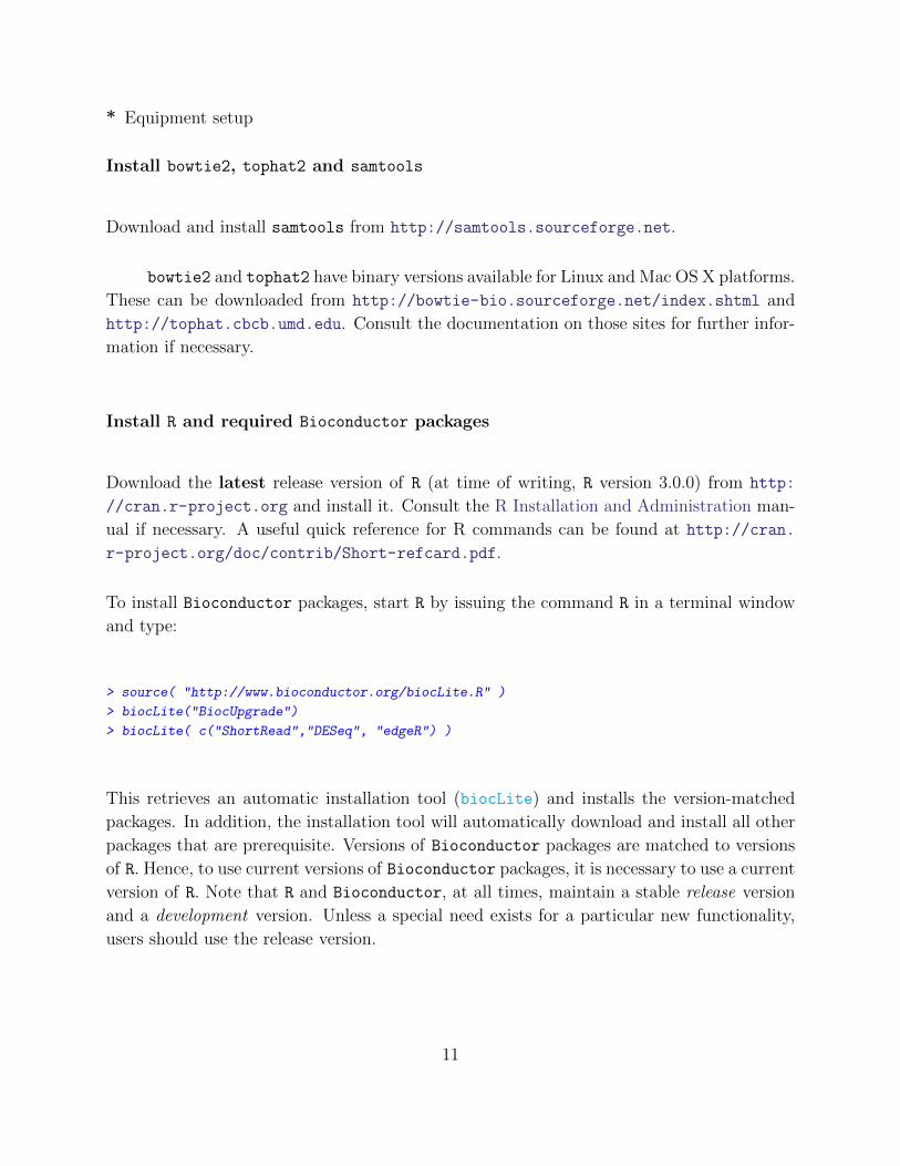
* Equipment setup

Install bowtie2, tophat2 and samtools

Download and install samtools from http://samtools.sourceforge.net.

bowtie2 and tophat2 have binary versions available for Linux and Mac OS X platforms.

These can be downloaded from http://bowtie-bio.sourceforge.net/index.shtml and

http://tophat.cbcb.umd.edu. Consult the documentation on those sites for further infor-

mation if necessary.

Install R and required Bioconductor packages

Download the latest release version of R (at time of writing, R version 3.0.0) from http:

//cran.r-project.org and install it. Consult the R Installation and Administration man-

ual if necessary. A useful quick reference for R commands can be found at http://cran.

r-project.org/doc/contrib/Short-refcard.pdf.

To install Bioconductor packages, start R by issuing the command R in a terminal window

and type:

> source( "http://www.bioconductor.org/biocLite.R" )

> biocLite("BiocUpgrade")

> biocLite( c("ShortRead","DESeq", "edgeR") )

This retrieves an automatic installation tool (biocLite) and installs the version-matched

packages. In addition, the installation tool will automatically download and install all other

packages that are prerequisite. Versions of Bioconductor packages are matched to versions

of R. Hence, to use current versions of Bioconductor packages, it is necessary to use a current

version of R. Note that R and Bioconductor, at all times, maintain a stable release version

and a development version. Unless a special need exists for a particular new functionality,

users should use the release version.

11

Download the example data

CRITICAL: This step is only required if data originate from the Short Read Archive (SRA).

Brooks et al. 51 deposited their data in the Short Read Archive (SRA) of the NCBI’s Gene

Expression Omnibus (GEO) 52 under accession number GSE18508 (http://www.ncbi.nlm.

nih.gov/geo/query/acc.cgi?acc=GSE18508), and a subset of this data set is used here to

illustrate the pipeline. Specifically, SRA files corresponding to the 4 “Untreated” (Control)

and 3 “CG8144 RNAi” (Knockdown) samples need to be downloaded.

For downloading SRA repository data, an automated process may be desirable. For example,

from http://www.ncbi.nlm.nih.gov/sra?term=SRP001537 (the entire experiment corre-

sponding to GEO accession GSE18508), users can download a table of the metadata into

a comma-separated tabular file “SraRunInfo.csv” (see Supplementary File 1, which contains

an archive of various files used in this protocol). To do this, click on “Send to:” (top right

corner), select “File”, select format “RunInfo” and click on “Create File”. Read this CSV file

“SraRunInfo.csv” into R, and select the subset of samples that we are interested in (using R’s

string matching function grep), corresponding to the 22 SRA files shown in Figure 2 by:

> sri = read.csv("SraRunInfo.csv", stringsAsFactors=FALSE)

> keep = grep("CG8144|Untreated-",sri$LibraryName)

> sri = sri[keep,]

The following R commands automate the download of the 22 SRA files to the current work-

ing directory (the functions getwd and setwd can be used to retrieve and set the working

directory, respectively):

> fs = basename(sri$download_path)

> for(i in 1:nrow(sri))

download.file(sri$download_path[i], fs[i])

The R-based download of files described above is just one way to capture several files in a

semi-automatic fashion. Users can alternatively use the batch tools wget (Unix/Linux) or

curl (Mac OS X), or download using a web browser. The (truncated) verbose output of the

above R download commands looks as follows:

12

trying URL 'ftp://ftp-private.ncbi.nlm.nih.gov/sra/sra-instant/reads/ByRun/sra/SRR/SRR031/SRR031714/SRR031714.sra'ftp data connection made, file length 415554366 bytes

opened URL

=================================================

downloaded 396.3 Mb

trying URL 'ftp://ftp-private.ncbi.nlm.nih.gov/sra/sra-instant/reads/ByRun/sra/SRR/SRR031/SRR031715/SRR031715.sra'ftp data connection made, file length 409390212 bytes

opened URL

================================================

downloaded 390.4 Mb

[... truncated ...]

Convert SRA to FASTQ format

Typically, sequencing data from a sequencing facility will come in (compressed) FASTQ

format. The SRA, however, uses its own, compressed, SRA format. To convert the example

data to FASTQ, use the fastq-dump command from the SRA Toolkit on each SRA file. R

can be used to construct the required shell commands, starting from the “SraRunInfo.csv”

metadata table, as follows:

> stopifnot( all(file.exists(fs)) ) # assure FTP download was successful

> for(f in fs) {

cmd = paste("fastq-dump --split-3", f)

cat(cmd,"\n")

system(cmd) # invoke command

}

CRITICAL: Using R’s system command is just one possibility. Users may choose to type the

22 fastq-dump commands manually into the Unix shell rather than using R to construct

them.

CRITICAL: It is not absolutely necessary to use cat to print out the current command, but

it serves the purpose of knowing what is currently running in the shell:

fastq-dump --split-3 SRR031714.sra

Written 5327425 spots for SRR031714.sra

13

Written 5327425 spots total

fastq-dump --split-3 SRR031715.sra

Written 5248396 spots for SRR031715.sra

Written 5248396 spots total

[... truncated ...]

CRITICAL: Be sure to use the --split-3 option, which splits mate-pair reads into separate

files. After this command, single and paired-end data will produce one or two FASTQ files,

respectively. For paired-end data, the file names will be suffixed 1.FASTQ and 2.FASTQ;

otherwise, a single file with extension .FASTQ will be produced.

Download the reference genome

Download reference genome sequence for the organism under study in (compressed) FASTA

format. Some useful resources, among others, include:

• the general Ensembl FTP server (http://www.ensembl.org/info/data/ftp/index.

html)

• the Ensembl plants FTP server (http://plants.ensembl.org/info/data/ftp/index.

html)

• the Ensembl metazoa FTP server (http://metazoa.ensembl.org/info/data/ftp/

index.html)

• the UCSC current genomes FTP server (ftp://hgdownload.cse.ucsc.edu/goldenPath/

currentGenomes/)

For Ensembl, choose the “FASTA (DNA)” link instead of “FASTA (cDNA)”, since alignments

to the genome, not the transcriptome, are desired. For Drosphila melanogaster, the file

labeled “toplevel” combines all chromosomes. Do not use the “repeat-masked” files (indicated

by “rm” in the file name), since handling repeat regions should be left to the alignment

algorithm.

The Drosophila reference genome can be downloaded from Ensembl and uncompressed using

the following Unix commands:

14

wget ftp://ftp.ensembl.org/pub/release-70/fasta/drosophila_melanogaster/\

dna/Drosophila_melanogaster.BDGP5.70.dna.toplevel.fa.gz

gunzip Drosophila_melanogaster.BDGP5.70.dna.toplevel.fa.gz

For genomes provided by UCSC, users can select their genome of interest, proceed to the

“bigZips” directory and download the “chromFa.tar.gz”; as above, this could be done using

the wget command. Note that bowtie2/tophat2 indices for many commonly used reference

genomes can be downloaded directly from http://tophat.cbcb.umd.edu/igenomes.html.

Get gene model annotations

Download a GTF file with gene models for the organism of interest. For species covered by

Ensembl, the Ensembl FTP site mentioned above contains links to such files.

The gene model annotation for Drosophila melanogaster can be downloaded and uncom-

pressed using:

wget ftp://ftp.ensembl.org/pub/release-70/gtf/drosophila_melanogaster/\

Drosophila_melanogaster.BDGP5.70.gtf.gz

gunzip Drosophila_melanogaster.BDGP5.70.gtf.gz

CRITICAL: Make sure that the gene annotation uses the same coordinate system as the

reference FASTA file. Here, both files use BDGP5 (i. e., release 5 of the assembly provided

by the Berkeley Drosophila Genome Project), as is apparent from the file names. To be on

the safe side here, we recommend to always download the FASTA reference sequence and the

GTF annotation data from the same resource provider.

CRITICAL: As an alternative, the UCSC Table Browser (http://genome.ucsc.edu/cgi-bin/

hgTables) can be used to generate GTF files based on a selected annotation (e. g., RefSeq

genes). However, at the time of writing GTF files obtained from the UCSC Table Browser

do not contain correct gene IDs, which causes problems with downstream tools such as

htseq-count, unless corrected manually.

15

Build the reference index

Before reads can be aligned, the reference FASTA files need to be preprocessed into an index

that allows the aligner easy access. To build a bowtie2-specific index from the FASTA file

mentioned above, use the command:

bowtie2-build -f Drosophila_melanogaster.BDGP5.70.dna.toplevel.fa Dme1_BDGP5_70

A set of BT2 files will be produced, with names starting with Dme1 BDGP5 70 as specfied

above. This procedure needs to be run only once for each reference genome used. As

mentioned, pre-built indices for many commonly-used genomes are available from http:

//tophat.cbcb.umd.edu/igenomes.html.

PROCEDURE

Assess sequence quality control with ShortRead TIMING:∼2 hours

1. At the R prompt, type the commands (you may first need to use setwd to set the working

directory to where the FASTQ files are situated):

> library("ShortRead")

> fqQC = qa(dirPath=".", pattern=".fastq$", type="fastq")

> report(fqQC, type="html", dest="fastqQAreport")

2. Use a web browser to inspect the generated HTML file (here, stored in the“fastqQAreport”

directory) with the quality-assessment report.

Collect metadata of experimental design

16

3. Create a table of metadata called samples (see Constructing metadata table). This

step needs to be adapted for each data set, and many users may find a spreadsheet program

useful for this step, from which data can be imported into the table samples by the read.csv

function. For our example data, we chose to construct the samples table programmatically

from the table of SRA files.

4. Collapse the initial table sri to one row per sample:

> sri$LibraryName = gsub("S2_DRSC_","",sri$LibraryName) # trim label

> samples = unique(sri[,c("LibraryName","LibraryLayout")])

> for(i in seq_len(nrow(samples))) {

rw = (sri$LibraryName==samples$LibraryName[i])

if(samples$LibraryLayout[i]=="PAIRED") {

samples$fastq1[i] = paste0(sri$Run[rw],"_1.fastq",collapse=",")

samples$fastq2[i] = paste0(sri$Run[rw],"_2.fastq",collapse=",")

} else {

samples$fastq1[i] = paste0(sri$Run[rw],".fastq",collapse=",")

samples$fastq2[i] = ""

}

}

5. Add important or descriptive columns to the metadata table (here, experimental group-

ings are set based on the “LibraryName” column, and a label is created for plotting):

> samples$condition = "CTL"

> samples$condition[grep("RNAi",samples$LibraryName)] = "KD"

> samples$shortname = paste( substr(samples$condition,1,2),

substr(samples$LibraryLayout,1,2),

seq_len(nrow(samples)), sep=".")

6. Since the downstream statistical analysis of differential expression relies on this table,

carefully inspect (and correct, if necessary) the metadata table. In particular, verify that

17

there exists one row per sample, that all columns of information are populated and the files

names, labels and experimental conditions are correct.

> samples

LibraryName LibraryLayout fastq1 fastq2 condition shortname

1 Untreated-3 PAIRED SRR031714_1.fastq,... SRR031714_2.fastq,... CTL CT.PA.1

2 Untreated-4 PAIRED SRR031716_1.fastq,... SRR031716_2.fastq,... CTL CT.PA.2

3 CG8144_RNAi-3 PAIRED SRR031724_1.fastq,... SRR031724_2.fastq,... KD KD.PA.3

4 CG8144_RNAi-4 PAIRED SRR031726_1.fastq,... SRR031726_2.fastq,... KD KD.PA.4

5 Untreated-1 SINGLE SRR031708.fastq,... CTL CT.SI.5

6 CG8144_RNAi-1 SINGLE SRR031718.fastq,... KD KD.SI.6

7 Untreated-6 SINGLE SRR031728.fastq,... CTL CT.SI.7

Align the reads (using tophat2) to reference genome TIMING:∼45 minutes per

sample

7. Using R string manipulation, construct the Unix commands to call tophat2. Given the

metadata table samples, it is convenient to use R to create the list of shell commands, as

follows:

> gf = "Drosophila_melanogaster.BDGP5.70.gtf"

> bowind = "Dme1_BDGP5_70"

> cmd = with(samples,

paste("tophat -G", gf, "-p 5 -o", LibraryName, bowind,

fastq1, fastq2))

> cmd

tophat -G Drosophila_melanogaster.BDGP5.70.gtf -p 5 -o Untreated-3 Dme1_BDGP5_70 \

SRR031714_1.fastq,SRR031715_1.fastq SRR031714_2.fastq,SRR031715_2.fastq

18

tophat -G Drosophila_melanogaster.BDGP5.70.gtf -p 5 -o Untreated-4 Dme1_BDGP5_70 \

SRR031716_1.fastq,SRR031717_1.fastq SRR031716_2.fastq,SRR031717_2.fastq

tophat -G Drosophila_melanogaster.BDGP5.70.gtf -p 5 -o CG8144_RNAi-3 Dme1_BDGP5_70 \

SRR031724_1.fastq,SRR031725_1.fastq SRR031724_2.fastq,SRR031725_2.fastq

tophat -G Drosophila_melanogaster.BDGP5.70.gtf -p 5 -o CG8144_RNAi-4 Dme1_BDGP5_70 \

SRR031726_1.fastq,SRR031727_1.fastq SRR031726_2.fastq,SRR031727_2.fastq

tophat -G Drosophila_melanogaster.BDGP5.70.gtf -p 5 -o Untreated-1 Dme1_BDGP5_70 \

SRR031708.fastq,SRR031709.fastq,SRR031710.fastq,SRR031711.fastq,SRR031712.fastq,SRR031713.fastq

tophat -G Drosophila_melanogaster.BDGP5.70.gtf -p 5 -o CG8144_RNAi-1 Dme1_BDGP5_70 \

SRR031718.fastq,SRR031719.fastq,SRR031720.fastq,SRR031721.fastq,SRR031722.fastq,SRR031723.fastq

tophat -G Drosophila_melanogaster.BDGP5.70.gtf -p 5 -o Untreated-6 Dme1_BDGP5_70 \

SRR031728.fastq,SRR031729.fastq

CRITICAL: In the call to tophat2, the option -G points tophat2 to a GTF file of annotation

to facilitate mapping reads across exon-exon junctions (some of which can be found de novo),

-o specifies the output directory, -p specifies the number of threads to use (this may affect

run times and can vary depending on the resources available). Other parameters can be

specified here, as needed; see the appropriate documentation for the tool and version you

are using. The first argument, Dmel_BDGP5_70 is the name of the index (built in advance),

and the second argument is a list of all FASTQ files with reads for the sample. Note that the

FASTQ files are concatenated with commas, without spaces. For experiments with paired-end

reads, pairs of FASTQ files are given as separate arguments and the order in both arguments

must match.

8. Run these commands (i.e. copy-and-paste) in a Unix terminal.

CRITICAL: Many similar possibilities exist for this step. Users can use the R function system

to execute these commands direct from R, cut-and-paste the commands into a separate Unix

shell or store the list of commands in a text file and use the Unix source command. In

addition, users could construct the unix commands independent of R.

Organize, sort and index the BAM files and create SAM files TIMING:∼1 hour

19

9. Organize the BAM files into a single directory, sort and index them and create SAM files,

by running the following R-generated commands:

> for(i in seq_len(nrow(samples))) {

lib = samples$LibraryName[i]

ob = file.path(lib, "accepted_hits.bam")

# sort by name, convert to SAM for htseq-count

cat(paste0("samtools sort -n ",ob," ",lib,"_sn"),"\n")

cat(paste0("samtools view -o ",lib,"_sn.sam ",lib,"_sn.bam"),"\n")

# sort by position and index for IGV

cat(paste0("samtools sort ",ob," ",lib,"_s"),"\n")

cat(paste0("samtools index ",lib,"_s.bam"),"\n\n")

}

samtools sort -n Untreated-3/accepted_hits.bam Untreated-3_sn

samtools view -o Untreated-3_sn.sam Untreated-3_sn.bam

samtools sort Untreated-3/accepted_hits.bam Untreated-3_s

samtools index Untreated-3_s.bam

samtools sort -n Untreated-4/accepted_hits.bam Untreated-4_sn

samtools view -o Untreated-4_sn.sam Untreated-4_sn.bam

samtools sort Untreated-4/accepted_hits.bam Untreated-4_s

samtools index Untreated-4_s.bam

samtools sort -n CG8144_RNAi-3/accepted_hits.bam CG8144_RNAi-3_sn

samtools view -o CG8144_RNAi-3_sn.sam CG8144_RNAi-3_sn.bam

samtools sort CG8144_RNAi-3/accepted_hits.bam CG8144_RNAi-3_s

samtools index CG8144_RNAi-3_s.bam

samtools sort -n CG8144_RNAi-4/accepted_hits.bam CG8144_RNAi-4_sn

samtools view -o CG8144_RNAi-4_sn.sam CG8144_RNAi-4_sn.bam

samtools sort CG8144_RNAi-4/accepted_hits.bam CG8144_RNAi-4_s

samtools index CG8144_RNAi-4_s.bam

samtools sort -n Untreated-1/accepted_hits.bam Untreated-1_sn

samtools view -o Untreated-1_sn.sam Untreated-1_sn.bam

samtools sort Untreated-1/accepted_hits.bam Untreated-1_s

samtools index Untreated-1_s.bam

samtools sort -n CG8144_RNAi-1/accepted_hits.bam CG8144_RNAi-1_sn

20

samtools view -o CG8144_RNAi-1_sn.sam CG8144_RNAi-1_sn.bam

samtools sort CG8144_RNAi-1/accepted_hits.bam CG8144_RNAi-1_s

samtools index CG8144_RNAi-1_s.bam

samtools sort -n Untreated-6/accepted_hits.bam Untreated-6_sn

samtools view -o Untreated-6_sn.sam Untreated-6_sn.bam

samtools sort Untreated-6/accepted_hits.bam Untreated-6_s

samtools index Untreated-6_s.bam

CRITICAL: Users should be conscious of the disk space that may get used in these op-

erations. In the command above, sorted-by-name SAM and BAM files (for htseq-count),

as well as a sorted-by-chromosome-position BAM file (for IGV) are created for each original

accepted hits.bam file. User may wish to delete (some of) these files after the steps below.

Inspect alignments with IGV

10. Start IGV, select the correct genome (here, D. melanogaster (dm3)) and load the BAM

files (with s in the filename) as well as the GTF file.

11. Zoom in on an expressed transcript until individual reads are shown and check whether

the reads align at and across exon-exon junctions, as expected given the annotation (See

example in Figure 3).

12. If any positive and negative controls are known for the system under study (e.g. known

differential expression), direct the IGV browser to these regions to confirm that the relative

read density is different according to expectation.

Count reads using htseq-count TIMING:∼3 hours

13. Add the names of the COUNT files to the metadata table and call HTSeq from the

21

following R-generated Unix commands:

> samples$countf = paste(samples$LibraryName, "count", sep=".")

> gf = "Drosophila_melanogaster.BDGP5.70.gtf"

> cmd = paste0("htseq-count -s no -a 10 ", samples$LibraryName, "_sn.sam ",

gf," > ", samples$countf)

> cmd

htseq-count -s no -a 10 Untreated-3_sn.sam \

Drosophila_melanogaster.BDGP5.70.gtf > Untreated-3.count

htseq-count -s no -a 10 Untreated-4_sn.sam \

Drosophila_melanogaster.BDGP5.70.gtf > Untreated-4.count

htseq-count -s no -a 10 CG8144_RNAi-3_sn.sam \

Drosophila_melanogaster.BDGP5.70.gtf > CG8144_RNAi-3.count

htseq-count -s no -a 10 CG8144_RNAi-4_sn.sam \

Drosophila_melanogaster.BDGP5.70.gtf > CG8144_RNAi-4.count

htseq-count -s no -a 10 Untreated-1_sn.sam \

Drosophila_melanogaster.BDGP5.70.gtf > Untreated-1.count

htseq-count -s no -a 10 CG8144_RNAi-1_sn.sam \

Drosophila_melanogaster.BDGP5.70.gtf > CG8144_RNAi-1.count

htseq-count -s no -a 10 Untreated-6_sn.sam \

Drosophila_melanogaster.BDGP5.70.gtf > Untreated-6.count

CRITICAL: The option -s signifies that the data is not from a stranded protocol (this may

vary by experiment) and the -a option specifies a minimum score for the alignment quality.

14. For differential expression analysis with edgeR, follow option A for simple designs and

option B for complex designs; for differential expression analysis with DESeq, follow option

C for simple designs and option D for complex designs.

22

A. edgeR - simple design

i) Load the edgeR package and use the utility function, readDGE, to read in the COUNT

files created from htseq-count:

> library("edgeR")

> counts = readDGE(samples$countf)$counts

ii) Filter lowly expressed and non-informative (e. g., non-aligned) features using a command

like:

> noint = rownames(counts) %in%

c("no_feature","ambiguous","too_low_aQual",

"not_aligned","alignment_not_unique")

> cpms = cpm(counts)

> keep = rowSums(cpms>1)>=3 & !noint

> counts = counts[keep,]

CRITICAL: In edgeR, it is recommended to remove features without at least 1 read per

million in n of the samples, where n is the size of the smallest group of replicates (here,

n = 3 for the Knockdown group).

iii) Visualize and inspect the count table using:

> colnames(counts) = samples$shortname

> head( counts[,order(samples$condition)], 5 )

CT.PA.1 CT.PA.2 CT.SI.5 CT.SI.7 KD.PA.3 KD.PA.4 KD.SI.6

FBgn0000008 76 71 137 82 87 68 115

FBgn0000017 3498 3087 7014 3926 3029 3264 4322

FBgn0000018 240 306 613 485 288 307 528

FBgn0000032 611 672 1479 1351 694 757 1361

FBgn0000042 40048 49144 97565 99372 70574 72850 95760

iv) Create a DGEList object (edgeR’s container for RNA-seq count data), as follows:

> d = DGEList(counts=counts, group=samples$condition)

v) Estimate normalization factors using:

> d = calcNormFactors(d)

> d$samples

23

vi) Inspect the relationships between samples using a multidimensional scaling plot, as

shown in Figure 4A:

> plotMDS(d, labels=samples$shortname,

col=c("darkgreen","blue")[factor(samples$condition)])

vii) Estimate tagwise dispersion (simple design) using:

> d = estimateCommonDisp(d)

> d = estimateTagwiseDisp(d)

viii) Create a visual representation of the mean-variance relationship using the plotMeanVar

(shown in Figure 5A) and plotBCV (Figure 5B) functions, as follows:

> plotMeanVar(d, show.tagwise.vars=TRUE, NBline=TRUE)

> plotBCV(d)

ix) Test for differential expression (“classic” edgeR), as follows:

> de = exactTest(d, pair=c("CTL","KD"))

x) Follow Step 14 B vi)-ix).

B. edgeR - complex design

i) Follow Step 14 A i)-vi).

ii) Create a design matrix to specify the factors that are expected to affect expression levels:

> design = model.matrix( ~ LibraryLayout + condition, samples)

> design

(Intercept) LibraryLayoutSINGLE conditionKD

1 1 0 0

2 1 0 0

3 1 0 1

4 1 0 1

5 1 1 0

6 1 1 1

7 1 1 0

24

attr(,"assign")

[1] 0 1 2

attr(,"contrasts")

attr(,"contrasts")$LibraryLayout

[1] "contr.treatment"

attr(,"contrasts")$condition

[1] "contr.treatment"

iii) Estimate dispersion values, relative to the design matrix, using the Cox-Reid (CR)

adjusted likelihood 7,53, as follows:

> d2 = estimateGLMTrendedDisp(d, design)

> d2 = estimateGLMTagwiseDisp(d2, design)

iv) Given the design matrix and dispersion estimates, fit a GLM to each feature:

> f = glmFit(d2, design)

v) Perform a likelihood ratio test, specifying the difference of interest (here, Knockdown

versus Control, which corresponds to the 3rd column of the above design matrix):

> de = glmLRT(f, coef=3)

vi) Use the topTags function to present a tabular summary of the differential expression

statistics (Note: topTags operates on the output of exactTest or glmLRT, while only

the latter is shown here):

> tt = topTags(de, n=nrow(d))

> head(tt$table)

logFC logCPM LR PValue FDR

FBgn0039155 -4.61 5.87 902 3.96e-198 2.85e-194

FBgn0025111 2.87 6.86 641 2.17e-141 7.81e-138

FBgn0039827 -4.05 4.40 457 2.11e-101 5.07e-98

FBgn0035085 -2.58 5.59 408 9.31e-91 1.68e-87

FBgn0000071 2.65 4.73 365 2.46e-81 3.54e-78

FBgn0003360 -3.12 8.42 359 3.62e-80 4.34e-77

vii) Inspect the depth-adjusted reads per million for some of the top differentially expressed

genes:

25

> nc = cpm(d, normalized.lib.sizes=TRUE)

> rn = rownames(tt$table)

> head(nc[rn,order(samples$condition)],5)

CT.PA.1 CT.PA.2 CT.SI.5 CT.SI.7 KD.PA.3 KD.PA.4 KD.SI.6

FBgn0039155 91.07 98.0 100.75 106.78 3.73 4.96 3.52

FBgn0025111 34.24 31.6 26.64 28.46 247.43 254.28 188.39

FBgn0039827 39.40 36.7 30.09 34.47 1.66 2.77 2.01

FBgn0035085 78.06 81.4 63.59 74.08 13.49 14.13 10.99

FBgn0000071 9.08 9.2 7.48 5.85 52.08 55.93 45.65

viii) Create a graphical summary, such as an M (log-fold-change) versus A (log-average-

expression) plot 54, here showing the genes selected as differentially expressed (with a

5% false discovery rate; see Figure 6A):

> deg = rn[tt$table$FDR < .05]

> plotSmear(d, de.tags=deg)

ix) Save the result table as a CSV (comma-separated values) file (alternative formats are

possible) as follows:

> write.csv(tt$table, file="toptags_edgeR.csv")

C. DESeq - simple design

i) Create a data.frame with the required metadata, i. e., the names of the count files and

experimental conditions. Here, we derive it from the samples table created earlier.

> samplesDESeq = with(samples, data.frame(

shortname = I(shortname),

countf = I(countf),

condition = condition,

LibraryLayout = LibraryLayout))

ii) Load the DESeq package and create a CountDataSet object (DESeq’s container for RNA-

seq data) from the count tables and corresponding metadata:

26

> library("DESeq")

> cds = newCountDataSetFromHTSeqCount(samplesDESeq)

iii) Estimate normalization factors using:

> cds = estimateSizeFactors(cds)

iv) Inspect the size factors using:

> sizeFactors(cds)

CT.PA.1 CT.PA.2 KD.PA.3 KD.PA.4 CT.SI.5 KD.SI.6 CT.SI.7

0.699 0.811 0.822 0.894 1.643 1.372 1.104

v) To inspect sample relationships, invoke a variance stabilizing transformation and inspect

a principal component analysis (PCA) plot (shown in Figure 4B):

> cdsB = estimateDispersions(cds, method="blind")

> vsd = varianceStabilizingTransformation(cdsB)

> p = plotPCA(vsd, intgroup=c("condition","LibraryLayout"))

vi) Use estimateDispersions to calculate dispersion values:

> cds = estimateDispersions(cds)

vii) Inspect the estimated dispersions using the plotDispEsts function (shown in Fig-

ure 5C), as follows:

> plotDispEsts(cds)

viii) Perform the test for differential expression, using nbinomTest, as follows:

> res = nbinomTest(cds,"CTL","KD")

ix) Given the table of differential expression results, use plotMA to display differential ex-

pression (log-fold-changes) versus expression strength (log-average-read-count), as fol-

lows (see Figure 6B):

> plotMA(res)

x) Inspect the result tables of significantly up- and down-regulated, at 10% FDR, using:

27

> resSig = res[which(res$padj < 0.1),]

> head( resSig[ order(resSig$log2FoldChange, decreasing=TRUE), ] )

id baseMean baseMeanA baseMeanB foldChange log2FoldChange pval padj

1515 FBgn0013696 1.46 0.000 3.40 Inf Inf 4.32e-03 6.86e-02

13260 FBgn0085822 1.93 0.152 4.29 28.2 4.82 4.54e-03 7.11e-02

13265 FBgn0085827 8.70 0.913 19.08 20.9 4.39 1.02e-09 9.57e-08

15470 FBgn0264344 3.59 0.531 7.68 14.5 3.86 4.55e-04 1.10e-02

8153 FBgn0037191 4.43 0.715 9.39 13.1 3.71 5.35e-05 1.78e-03

1507 FBgn0013688 23.82 4.230 49.95 11.8 3.56 3.91e-21 1.38e-18

> head( resSig[ order(resSig$log2FoldChange, decreasing=FALSE), ] )

id baseMean baseMeanA baseMeanB foldChange log2FoldChange pval padj

13045 FBgn0085359 60.0 102.2 3.78 0.0370 -4.76 7.65e-30 4.88e-27

9499 FBgn0039155 684.1 1161.5 47.59 0.0410 -4.61 3.05e-152 3.88e-148

2226 FBgn0024288 52.6 88.9 4.25 0.0478 -4.39 2.95e-32 2.09e-29

9967 FBgn0039827 246.2 412.0 25.08 0.0609 -4.04 1.95e-82 8.28e-79

6279 FBgn0034434 104.5 171.8 14.72 0.0856 -3.55 8.85e-42 9.40e-39

6494 FBgn0034736 203.9 334.9 29.38 0.0877 -3.51 6.00e-41 5.88e-38

xi) Count the number of genes with significant differential expression at FDR of 10%:

> table( res$padj < 0.1 )

FALSE TRUE

11861 885

xii) Create persistent storage of results using, for example, a CSV file:

> write.csv(res, file="res_DESeq.csv")

xiii) Perform a sanity check by inspecting a histogram of unadjusted p-values (see Figure 7)

for the differential expression results, as follows:

> hist(res$pval, breaks=100)

28

D. DESeq - complex design

i) Follow Step 14 C i)-v).

ii) Calculate the CR adjusted profile likelihood 53 dispersion estimates relative to the factors

specified, developed by McCarthy et al. 7, according to:

> cds = estimateDispersions(cds, method = "pooled-CR",

modelFormula = count ~ LibraryLayout + condition)

iii) Test for differential expression in the GLM setting by fitting both a full model and

reduced model (i. e., with the factor of interest taken out):

> fit1 = fitNbinomGLMs(cds, count ~ LibraryLayout + condition)

> fit0 = fitNbinomGLMs(cds, count ~ LibraryLayout)

iv) Using the two fitted models, compute likelihood ratio statistics and associated P-values,

as follows:

> pval = nbinomGLMTest(fit1, fit0)

v) Adjust the reported p values for multiple testing:

> padj = p.adjust(pval, method="BH")

vi) Assemble a result table from full model fit and the raw and adjusted P-values and print

the first few up- and down-regulated genes (FDR less than 10%):

> res = cbind(fit1, pval=pval, padj=padj)

> resSig = res[which(res$padj < 0.1),]

> head( resSig[ order(resSig$conditionKD, decreasing=TRUE), ] )

(Intercept) LibraryLayoutSINGLE conditionKD deviance converged pval padj

FBgn0013696 -70.96 36.829 37.48 5.79e-10 TRUE 3.52e-03 5.51e-02

FBgn0085822 -5.95 4.382 5.14 2.07e+00 TRUE 4.72e-03 7.07e-02

FBgn0085827 -3.96 4.779 5.08 2.89e+00 TRUE 5.60e-03 8.05e-02

FBgn0264344 -2.59 2.506 4.26 6.13e-01 TRUE 3.86e-04 9.17e-03

FBgn0261673 3.53 0.133 3.37 1.39e+00 TRUE 0.00e+00 0.00e+00

FBgn0033065 2.85 -0.421 3.03 4.07e+00 TRUE 8.66e-15 1.53e-12

> head( resSig[ order(resSig$conditionKD, decreasing=FALSE), ] )

29

(Intercept) LibraryLayoutSINGLE conditionKD deviance converged pval padj

FBgn0031923 1.01 1.2985 -32.26 1.30 TRUE 0.00528 0.077

FBgn0085359 6.37 0.5782 -4.62 3.32 TRUE 0.00000 0.000

FBgn0039155 10.16 0.0348 -4.62 3.39 TRUE 0.00000 0.000

FBgn0024288 6.71 -0.4840 -4.55 1.98 TRUE 0.00000 0.000

FBgn0039827 8.79 -0.2272 -4.06 2.87 TRUE 0.00000 0.000

FBgn0034736 8.54 -0.3123 -3.57 2.09 TRUE 0.00000 0.000

vii) Follow Step 14 C xi)-xiii).

15. As another spot check, point the IGV genome browser (with GTF and BAM files loaded)

to a handful of the top differentially expressed genes and confirm that the counting and

differential expression statistics are appropriately represented.

TIMING

Running this protocol on the SRA-downloaded data will take ∼10 hours on a machine

with eight cores and 8 GB of RAM; with a machine with more cores, mapping of different

samples can be run simultaneously. The time is largely spent on quality checks of reads, read

alignment and feature counting; computation time for the differential expression analysis is

comparatively smaller.

Step 1, Sequence quality checks, ∼2 h

Step 3-6, Organizing metadata: ∼<1 h

Steps 7-8, Read alignment: ∼6 h

Step 13, Feature counting: ∼3 h

Step 14, Differential analysis: variable; computational time is often <20 min

TROUBLESHOOTING

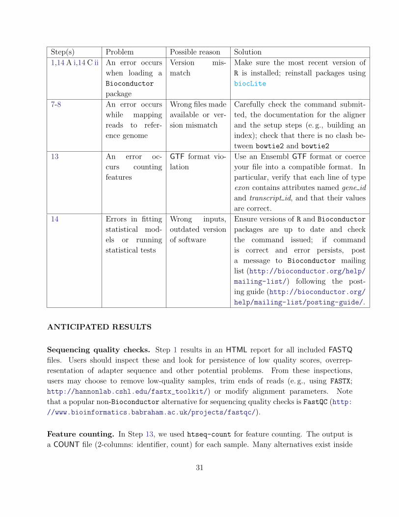
Troubleshooting advice can be found in Table 1.

Table 1. Troubleshooting

30

Step(s) Problem Possible reason Solution

1,14 A i,14 C ii An error occurs

when loading a

Bioconductor

package

Version mis-

match

Make sure the most recent version of

R is installed; reinstall packages using

biocLite

7-8 An error occurs

while mapping

reads to refer-

ence genome

Wrong files made

available or ver-

sion mismatch

Carefully check the command submit-

ted, the documentation for the aligner

and the setup steps (e. g., building an

index); check that there is no clash be-

tween bowtie2 and bowtie2

13 An error oc-

curs counting

features

GTF format vio-

lation

Use an Ensembl GTF format or coerce

your file into a compatible format. In

particular, verify that each line of type

exon contains attributes named gene id

and transcript id, and that their values

are correct.

14 Errors in fitting

statistical mod-

els or running

statistical tests

Wrong inputs,

outdated version

of software

Ensure versions of R and Bioconductor

packages are up to date and check

the command issued; if command

is correct and error persists, post

a message to Bioconductor mailing

list (http://bioconductor.org/help/

mailing-list/) following the post-

ing guide (http://bioconductor.org/

help/mailing-list/posting-guide/.

ANTICIPATED RESULTS

Sequencing quality checks. Step 1 results in an HTML report for all included FASTQ

files. Users should inspect these and look for persistence of low quality scores, overrep-

resentation of adapter sequence and other potential problems. From these inspections,

users may choose to remove low-quality samples, trim ends of reads (e. g., using FASTX;

http://hannonlab.cshl.edu/fastx_toolkit/) or modify alignment parameters. Note

that a popular non-Bioconductor alternative for sequencing quality checks is FastQC (http:

//www.bioinformatics.babraham.ac.uk/projects/fastqc/).

Feature counting. In Step 13, we used htseq-count for feature counting. The output is

a COUNT file (2-columns: identifier, count) for each sample. Many alternatives exist inside

31

and outside of Bioconductor to arrive at a table of counts given BAM (or SAM) files and a

set of features (e. g., from a GTF file); see Box 3 for further considerations. Each cell in the

count table will be an integer that indicates how many reads in the sample overlap with the

respective feature. Non-informative rows, such as features that are not of interest or those

that have low overall counts can be filtered. Such filtering (so long as it is independent of

the test statistic) is typically beneficial for the statistical power of the subsequent differential

expression analysis 55.

“Normalization”. As different libraries will be sequenced to different depths, the count

data are scaled (in the statistical model) so as to be comparable. The term normalization is

often used for that, but it should be noted that the raw read counts are not actually altered 56.

By default, edgeR uses the number of mapped reads (i. e., count table column sums) and

estimates an additional normalization factor to account for sample-specific effects (e. g., diver-

sity) 56; these two factors are combined and used as an offset in the NB model. Analagously,

DESeq defines a virtual reference sample by taking the median of each gene’s values across

samples, and then computes size factors as the median of ratios of each sample to the refer-

ence sample. Generally, the ratios of the size factors should roughly match the ratios of the

library sizes. Dividing each column of the count table by the corresponding size factor yields

normalized count values, which can be scaled to give a counts per million interpretation (see

also edgeR’s cpm function). From an M (log-ratio) versus A (log-expression-strength) plot,

count datasets typically show a (left-facing) trombone shape, reflecting the higher variability

of log-ratios at lower counts (See Figure 6). In addition, points will typically be centered

around a log-ratio of 0 if the normalization factors are calculated appropriately, although

this is just a general guide.

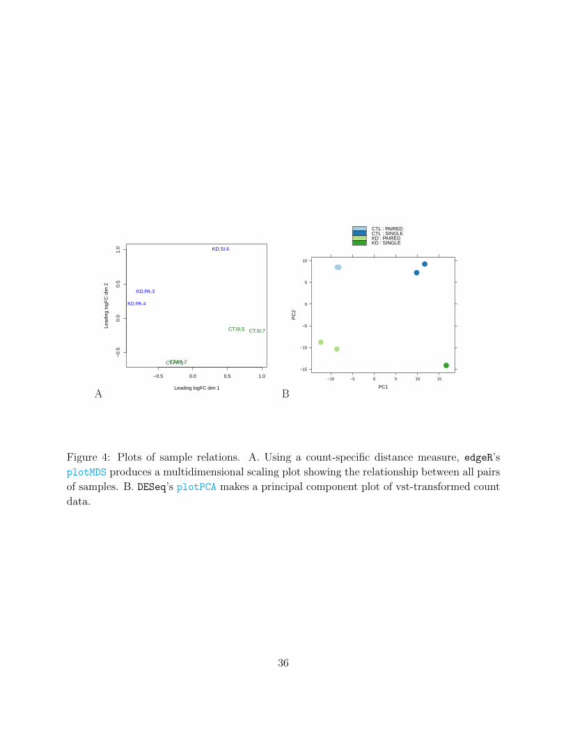
Sample relations. The quality of the sequencing reactions (Step 1) themselves are only part

of the quality assessment procedure. In Steps 14 A vi or 14 C v, a “fitness for use”57 check

is performed (relative to the biological question of interest) on the count data before sta-

tistical modeling. edgeR adopts a straightforward approach that compares the relationship

between all pairs of samples, using a count-specific pairwise distance measure (i. e., biolog-

ical coefficient of variation) and an MDS plot for visualization (Figure 4A). Analagously,

DESeq performs a variance-stabilizing transformation and explores sample relationships us-

ing a PCA plot (Figure 4B). In either case, the analysis for the current data set highlights

that library type (single-end or paired-end) has a systematic effect on the read counts and

provides an example of a data-driven modeling decision: here, a GLM-based analysis that

accounts for the (assumed linear) effect of library type jointly with the biological factor

of interest (i. e., Knockdown versus Control) is recommended. In general, users should be

conscious that the degree of variability between biological replicates (e. g., in an MDS or

32

PCA plot) will ultimately impact the calling of differential expression. For example, a single

outlying sample may drive increased dispersion estimates and compromise the discovery of

differentially expressed features. No general prescription is available for when and whether

to delete outlying samples.

Dispersion estimation. As mentioned above, getting good estimates of the dispersion

parameter is critical to the inference of differential expression. For simple designs, edgeR

uses the quantile-adjusted conditional maximum (weighted) likelihood estimator 4,5, whereas

DESeq uses a method-of-moments estimator 3. For complex designs, the dispersion estimates

are made relative to the design matrix, using the CR adjusted likelihood 7,53; both DESeq and

edgeR use this estimator. edgeR’s estimates are always moderated toward a common trend,

whereas DESeq chooses the maximum of the individual estimate and a smooth fit (dispersion

versus mean) over all genes. A wide range of dispersion-mean relationships exist in RNA-seq

data, as viewed by edgeR’s plotBCV or DESeq’s plotDispEsts; case studies with further

details are presented in both edgeR’s and DESeq’s user guides.

Differential expression analysis. DESeq and edgeR differ slightly in the format of re-

sults outputted, but each contain columns for (log) fold change, (log) counts-per-million (or

mean by condition), likelihood ratio statistic (for GLM-based analyses), as well as raw and

adjusted P-values. By default, P-values are adjusted for multiple testing using the Benjamini-

Hochberg 58 procedure. If users enter tabular information to accompany the set of features

(e.g. annotation information), edgeR has a facility to carry feature-level information into the

results table.

Post differential analysis sanity checks. Figure 7 (Step 14 C xiii) shows the typical

features of a P -value histogram resulting from a good data set: a sharp peak at the left side,

containing genes with strong differential expression, a“floor”of values that are approximately

uniform in the interval [0, 1], corresponding to genes that are not differentially expressed

(for which the null hypothesis is true), and a peak at the upper end, at 1, resulting from

discreteness of the Negative Binomial test for genes with overall low counts. The latter

component is often less pronounced, or even absent, when the likelihood ratio test is used.

In addition, users should spot check genes called as differentially expressed by loading the

sorted BAM files into a genome browser.

FIGURE LEGENDS

**** START BOX 1:

33

Figure 1: Count-based differential expression pipeline for RNA-seq data using edgeR and/or

DESeq. Many steps are common to both tools, while the specific commands are different (Step

14). Steps within the edgeR or DESeq differential analysis can follow two paths, depending

on whether the experimental design is simple or complex. Alternative entry points to the

protocol are shown in orange boxes.

34

Figure 2: Metadata available from Short Read Archive.

Figure 3: Screenshot of reads aligning across exon junctions.

35

A

−0.5 0.0 0.5 1.0

−0.

50.

00.

51.

0

Leading logFC dim 1

Lead

ing

logF

C d

im 2

CT.PA.1CT.PA.2

KD.PA.3

KD.PA.4

CT.SI.5

KD.SI.6

CT.SI.7

B

CTL : PAIREDCTL : SINGLEKD : PAIREDKD : SINGLE

PC1

PC

2

−15

−10

−5

0

5

10

−10 −5 0 5 10 15

●●●

●

●●

●

Figure 4: Plots of sample relations. A. Using a count-specific distance measure, edgeR’s

plotMDS produces a multidimensional scaling plot showing the relationship between all pairs

of samples. B. DESeq’s plotPCA makes a principal component plot of vst-transformed count

data.

36

A

●

●

●

●

●

●

●●

●●

●

●

●

●

●

●

●

●

●

●

●

●

●

●

●●

●

●

●

●

●

●

●

●

●●

●

●

●

●

●

●

●

●

●●

●

●

●

●

●

●

●

●

●

●

●

●

●

●

●

●

●

●

●

●●

●

●

●

●

●

●

●●●

●●

●●

●

●

●●

●

●

●●

●

●

●

●

●

●

●

●

●●

●

●

●

●

●

●●

●

●

●

●

●

●●

●

●

●

●

●

●

●

●

●

●

●

●

●

●

●

●

●

●

●

●

●

●

●

●

●

●

●

●

●

●

●

●

●

●

●

●

●

●

●●

●

●

●●●

●

●

●●

●

●●

●

●

●

●

●

●

●

●

●

●

●

●

●

●

●

●

●

●

●

●

●

●

●

●

●

●

●

●

●

●

●

●

●

●

●

●

●

●

●

●

●

●

●

●

●

●

●

●

●

●

●

●

●

●

●

●

●

●

●

●

●

●

●

●

●●

●

●

●

●

●

●

●

●

●

●

●

●●

●

●

●

●●

●

●

●

●

●

●

●

●

●

●●

●

●

●

●

●

●

●

●

●

●

●

●

●

●

●

●

●

●●

●

●

●

●

●

●

●●

●

●

●●

●

●

●

●

●

●

●

●

●

●

●

●

●

●

●●

●

●

●

●

●

●

●

●

●

●

●●

●

●

●

●●

●

●

●

●

●

●

●

●

●

●

●

●

●

●

●

●●

●

●

●

●

●

●

●

●

●

●

●

●

●

●

●

●

●●●

●●

●

●

●

●

●

●

●

●

●

●

●

●

●

●

●

●

●

●

●

●

●●

●

●

●

●

●

●

●

●

●

●

●

●

●

●

●

●

●

●

●

●●●

●

●

●

●

●

●

●

●

●

●

●

●

●

●

●

●

●

●●

●

●

●

●

●

●

●

●

●

●

●

●

●●

●

●

●

●

●●

●

●

●

●●

●

●●

●●

●

●

●

●

●

●

●●

●

●

●

●●

●

●

●

●

●

●

●

●

●

●

●

●

●

●

●●

●

●●

●

●

● ●

●

●

●

●

●

●

●

●● ●

●

●

●●

●

●

●●

●●

●●

●

●

●

●

●

●

●

●

●

●

●

●

●

●

●

●

●

●

●●

●

●

●●

●

●

●

●●

●

●

●

●

●

●●●

●

●

●

●

●

●

●

●

●

●

●

●

●●

●

●

●

●

●

●

●

●●

●

●

●

●●

●

●

●

●

●

●

●

●

●

●

●

●

●

●●

●

●

●

●

●

●

●

●

●●

●

●

●

●●●

●

●

●

●

●

●

●

●●

●

●●

●

●

●

●

●

●

●

●

●

●

●

●

●●

●

●

●

●

●●

●

●

●

●

●●

●

●

●

●

●●

●

●

●

●●

●

●

●

●

●

●

●

●

●

●

●

●

●

●

●

●

●

●

●

●

●

●

●●●

●

●

●

●

●

●

●

●

●●

●

●

●

●

●

●

●

●

●

●

●

●

●●

●●

●

●

●

●

●

●

●

●●

●

●

●

●

●

●

●

●

●

●

●●

●

●

●

●

●

●

●

●

●

●●

●●

●

●

●

●

●●

●

●

●

●

●

●

●

●

●

●

●

●

●

●

●

●

●

●

●

●●

●

●

●

●

●

●

●

●

●

●

●

●

●

●

●

●

●

●

●

●

●

●●

●

●

●

●

●

●

●●●

●

●

●

●

●

●

●

●

●●

●

●

●

●

●

●

●●

●

●

●

●

●

●

●

●

●

●

●

●

●●

●

●

●

●

●

●

●

●

●

●

●

●

●

●

●

●

●

●

●

●

●

●

●

●●

●

●

●

●

●

●

●

●●

●

●

●

●

●

●

●

●

●

●

●

●

●

●

●

●

●

●

●●

●

●●

●

●

●●

●

●

●

●

●

●●

●

●

●

●

●

●

●

●

●

●

●

●●

●

●

●

●

●

●

●●

●

●

●

●

●

●

●

●

●

●

●

●

●

●

●●

●

●

●

●

●

●

●

●●

●

●

●

●

●

●

●

●

●

●

●

●●●

●

●

●

●

●

●

●

●

●●

●

●

●

●

●

●

●●

●

●

●●●

●

●●

●

●

●

●

●●

●

●

●

●

●

●

●

●

●●

●

●

●

●

●

●●

●

●

●

●

●

●

●

●

●

●

●●

●

●

●

●

●

●

●●

●

●

●

●

●

●

●

●

●

●

●

●

●

●

●

●

●

●●

●●

●

●

●●

●

●

●

●

●●

●●

●

●

●

●

●

●●

●

●

●

●

●

●

●

●

●

●

●●

●

●

●

●

●

●

●●●

●

●

●●

●

●

●

●

●

●

●

●

●

●

●

●

●

●

●

●

●

●

●●

●

●

●

●

●

●

●

●

●

●

●

●

●

●●

●

●●

●

●

●

●

●

●

●●

●●

●

●

●

●●

●

●

●

●

●●

●

●

●

●

●

●

●

●

●

●

●

●

●

●

●

●●

●

●

●

●

●

●

●

●

●

●●

●●

●

●

●

●

●

●

●

●

●

●

●

●

●

●

●

●

●

●

● ●

●

●

●

●

●

●

●

● ●

●

●

●

●

●

●

●

●

●

●

●

●

●

●●

●

●

●

●●

●

●

●●

●●

●

●

●

●

●●

●●

●

●

●

●

●

●

●

●●

●

●

●

●

●

●

●

●

●●

●

●

●●

●

●●

●

●

●

●

●

●

●

●

●

●

●

●

●

●

●

●

●

●

●

●

●

●

●

●

●

●

●

●

●

●

●●

●

●●

●

●

●

●

●

●

●

●

●

●

●

●

●

●

●

●

●

●

●

●

●

●

●

●

●

●

●

●●

●●

●●

●

●

●

●

●

●

●

●●

●

●

●

●

●●

●

●

●

●

●

●

●

●

●

●

●

●

●

●●

●

●

●●

●

●

●

●

●

●

●

●

●

●

●

●

●

●

●

●

●

●

●●

●

●

●

●

●

●

●●

●●

●●

●

●

●

●

●

●

●

●●

●

●

●

●

●

●

●

●

●

●

●

●

●

●

●

●

●●●

●

●

●

●

●

●

●

●

●

●

●●

●

●●

●

●

●

●

●

●

●

●

●

●

●

●

●

●

●

●

●

●

●

●

●

●

●

●

●

●

●

●

●

●

●

●

●●

●

●

●

●

●

●

●

●

●

●

●

●

●

●

●

●

●

●

●

●

●

●

●

●

●

●

●

●

●

●

●

●

●

●●

●

●

●

●

●●

●

●

●

●

●

●●

●

●

●

●

●

●●

●

●

●●

●

●

●

●

●

●

●

●●

●

●

●

●

●

●●

●

●

●

●

●

●

●

●

●

●

●

●

●

●

●

●●

●

●

●

●

●

●

●

●

●

●

●

●

●

●

●

●

●

●

●

●

●

●

●

●

●

●

●

●

●

●

●

●

●

●

●

●

●

●

●

●

●

●

●

●

●

●

●●

●

●

●

●

●

●

●

●

●

●

●

●

●

●

●●●

●

●

●

●

●

●

●

●

●

●

●●

●

●

●

●

●●

●

●

●

●

●

●

●●

●

●

●

●

●

●

●

●

●●

●

●

●●●

●●●

●

●

●

●

●

●

●

●

●

●

●

●

●

●

●

●

●

●

●

●

●

●

●

●

●

●

●●

●

●

●

●

●

●●

●

●●

●

●

●

●

●●

●

●

●

●

●

●

●●

●

●

●

●

●●

●

●

●

●

●

●

●

●

●●

●

●●

●

●

●

●●●●

●

●

●

●

●

●

●

●

●

●

●

●●

●

●

●

●

●

●

●

●

●

●

●●

●

●

●

●

●

●

●

●

●●●●

●

●

●

●

●

●

●

●●

●

●

●

●

●●

●

●

●

●

●

●

●

●

●

●

●

●

●

●

●

●●

●

●

●

●

●

●

●

●

●

●

●

●

●●

●

●

●●

●

●

●

●

●

●

●

●

●● ●

●

●

●●

●

●

●

●

●

●

●

●

●

●

●

●

●

● ●

●

●

●

●

●

●

●

●

●

●●

●●

●

●

●●

●

●

●

●

●

●

●●

●

●

●

●

●

●

●●

●

●

●●

●

●

●

●

●

●

●

●

●

●

●

●●

●

●

●

●

●

●

●

●

●●

●

●

●

●

●

●

●

●

●

●

●

●

●

●

●●

●

●

●

●

●

●

● ●●

●

●

●

●

●

●

●

●

●

●

●

●

●●

●

●

●

●

●

●

●

●

●

●

●

●

●

●

●

●

●●

●

●

●

●

●

●

●

●●

●

●

●

●

●

●

●

●

●

●

●

●

●

●

●

●●

●

●

●

●

●

●

●

●

●

●

●

●

●●

●

●

●

●

●

●

●

●

●

●

●

●

●

●

●

●

●

●

●●

●

●

●

●

●

●

●

●

●

●

●

●

●

●

●

●

●

●

● ●

●

●

●

●

●

●

●

●

●

●

●

●

●

●

●

●

●

●

●

●

●

●

●

●

●

●

●

●

●●

●

●

●

●●

●

●

●

●

●

●

●●

●

●

●

●

●

●

●

●

●

●

●

●

●

●

●

●

●

●

●

●

●

●

●

●

●

●

●●

●

●

●●

●

●

●

●

●

●

●

●

●

●

●

●

●

●●

●

●

●

●

●

●

●

●

●

●

●

●

●

●

●

●

●

●

●

●

●

●

●

●

●●

●

●

●

●

●

●

●

●

●

●

●

●

●●

●

●

●

●

●

●

●

●

● ●

●

●

●

●

●

●

●

●

●

●

●

●

●

●

●

●

●

●

●

●

●

●

●

●

●

●

●

●

●●

●

●

●

●

●

●

●

●●

●

●

●

●

●●

●

●

●

●

●

●

●

●

●

●

●

●

●

●●

●●

●

●●

●

●

●●

●

●

●

●

●●

●

●

●●

●

●●

●

●●

●

●

●

●

●

●

●

●

●●

●

●

●

●

●

●

●

●

●

●

●

●●

●

●

●

●

●

●

●●

●

●

●

●

●

●

●

●

●

●

●●

●

●

●

●

●

●

●

●

●

●●

●

●

●

●

●

●

●

●

●

●●

●

●

●

●

●

●

●

●

●

●

●

●

●●

●

●

●

●

●

●

●

●●

●

●

●

●●

●

●●

●

●

●

●

●●

●

●

●

●

●

●

●

●

●

●

●

●

●

●

●

●

●

●●

●

●

●

●

●

●

●

●

●

●●

●●

●

●

●

●●●

●

●

●

●

●

●

●

●

●

●●

●

●

●

●

●

●

●

●

●

●

●

●

●

●●

●

●

●

●

●

●

●

●

●

●

●

●

●

●

●

●

●

●

●

●

●

●

●

●●

●

●

●

●

●●

●

●

●

●●

●

●

●

●

●

●

●

●

●

●

●

●

●

●

●

●

●

●

●

●

●

●●

●

●●

●

●

●

●

●

●

●

●

●

●●

● ●

●●

●

●

●

●

●

●

●

●

●

●

●

●

●

●

●

●●

●

●

●

●

●

●

●

●

●

●

●●

●

● ●

●●

●

●

●

●

●

●

●

●

●

●

●

●

●

●

●

●

●

●

●●

●

●

●

●

●

●●

●

●●

●●

●

●●

●

●

●●

●

●

●

●

●

●

●

●●

●

●

●

●

●

●

●●

●

●

●

●

●

●

●

●

●

●

●

●

●

●

●

●

●

●

●

●

●●

●

●

●

●

●

●

●

●

●

●

●

●

●

●

●●

● ●

●

●

●

●

●●

●

●

●●

●

●

●

●●

●

●

●

●

●

●

●

●

●●

●●

●●

●

●

●

●

●

●

●

●

●●

●

●

●

●

●

●●

●●

●

●

●

●●

●

●

●

●●

●

●

●

●●

●●

●●

●

●

●

●

●

●●

●●

●

●●

●

●

●

●●

●

●

●

●

●

●

●

●

●

●●

●

●

●

●●

●

●

●

●●

●

●

●

●

●

●●

●

●●

●

●

●

●

●

●

●

●

●

●

●

●●

●

●

●

●

●●

●

●

●

●●

●●

●

●●

●

●

●

●

●

●

●

●

●

●●

●●

●

●

●

●

● ●

●

●

●

●

●

●

●

●

●

●

●

●

●

●

●

●

●

●

●●

●

●

●●

●

●

●

●

●

●

●

●

●

●

●

●

●

●

●

●

●

●●

●

●

●

●

●

●

●

●

●

●

●

●

●

●

●

●

●●

●

●

●

●

●

●

●

●●

●

●

●

●

●

●

●●

●

●

●

●

●

●

●

●

●

●●

●

●

●

●

●

●

●

●

●

●●

●

●

●

●

●

●

●

●

●

●

●

●

●

●

●

●

●

●

●

●

●

●

●●

●

●

●

●

●

●

●

●

●●

●

●

●

●

●

●

●

●

●●

●●

●

●●

●

●

●

●

●

●

●

●

●

●

●●

● ●

●

●

●

●

●

●

●

●

●

●

●

●

●

●

●

●

●

●●

●

●

●

●

●

●

●

●

●

●

●

●

●

●

●

●

●

●

●

●

●

●

●

●

●

●

●

●

●

●

●

●

●

●

●

●

●

●

●

●

●●

●

●

●

●

●●●

●

●

●

●

●

●

●

●

●

●

●

●

●

●

●

●

●●

●

●

●

●●

●

●

●

●

●

●

●

●

●

●

●

●

●

●

●

●

●

●

●

●

●

●

●

●

●

●

●

●

●

●

●

●

●

●

●

●

● ●

●

●

●

●

●

●

●

●●

●●

●

●

●

●

●

●

●

●

●●

●

●

●

●

●

●

●

●●

●

●

●

●

●

●

●

●

●●●

●

●

●

●

●

●

●

●●

●

●

●

●

●

●

●

●

●

●

●

●●

●

●

●

●●

●

●

●

●

●

●

●●

●●

●

●

●

●

●

●

●

●

●

●

●

●

●

●

●

●●

●

●●

●

●

●

●

●

●

●

●●

●

●

●●

●

●

●

●

●

●

●

●

●

●

●

●

●

●

●

●●

●

●

●●

●●

●

●

●

●

●

●

●

●

●●

●

●

●

●

●

●

●

●

●

●

●●

●

●

●

●●

●

●

●●

●

●

●

●

●

●

●

●

●

●

●

●

●

●

●●

●

●

●

●

●

●

●

●

●

●

●

●

●

●

●

●

●

●

●●

●

●

●

●

●

●

●

●

●

●

●

●

●

●

●

●

●

●

●

●

●

●

●●

●

●●

●

●

●

● ●

●

●

●

●

●

●

●

●●

●

●

●

●

●

●

●

●

●●

●

●

●

●

●

●

●

●

●

●

●

●

●

●

●

●

●

●●●

●

●

●

●

●

●

●

●

●●

●

●

●

●●

●

●

●

●

●

●● ●

●

●

●

●

●

●

●

●

●

●

●

●

●

●

●

●

●

●

●

●

●

●

●●

●

●

●

●●●

●

●

●

●

●

●

●

●

●

●

●

●

●

●

●

●

●●

●

●

●

●

●

●

●

●

●

●

●

●●

●

●

●

●

●

●

●

●●

●

●●

●

●

●

●

●

●

●●

●

●

●

●

●

●

●

●

●

●

●

●

●

●

●

●●

●

●

●

●

●●

●

●

●●

●

●

●

●

●

●

●

●

●

●

●

●

●

●

●

●

●

●●

●

●

●

●

●

●

●

●●

●

●

●

●

●

●

●

●

●●

●

●

●

●

●

●

●

●

●

●

●

●

●

●●

●

●

●

●●

●

●

●

●

●

●

●

●

●

●

●

●

●

●

●

●

●

●

●

●

●

●

●

●

●

●

●

●

●

●

●

●

●●

●

●

●

●●

●

●

●

●●

●

●

●

●

● ●●

●

●

●

●

●

●

●

●

●

●

●

●

●

●

●

●

●●

●

●

●

●

●

●

●

●

●

●

●

●

●

●

●

●

●

●

●

●

●

●

●

●●

●

●

●

●

●

●

●

●

●

●●

●

●

●

●

●

●

●

●

●

●

●

●

●

●

●

●

●

●

●

●

●

●

●

●

●

●

●

●

●

●

●

●

●●

●

●

●

●

●●

●

●

●

●

●●

●

●

●

●

●

●

●●

●

●

●

●

●

●

●

●

●

●

●

●

●

●

●

●

●

●●

●

●●

●

●

●

●

●

●

●

●

●

●

●

●

●

●

●

●

●

●

●

●

●

●

●

●●

●●

●●

●

●

●●

●

●●

●

●

●

●

●

●

●

●

●

●●

●

●

●

●

●

●

●

●

●

●

●

●

●

●

●

●

●●

●

●

●

●

●

●

●●

●

●

●

●

●

●

●

●

●

●

●

●

●

●

●●

●

●

●

●

●

●

●

●●

●

●

●

●

●●

●●●

●

●

●

●

●

●

●

●

●

●

●

●

●

●

●

●

●

●

●

●

●

●

●●

●

●

●

●

●

●

●

●

●

●

●

●●

●

●

●●

●●

●

●

●

●●

●

●

●

●

●

●

● ●●

●

●

●

●

●

●

●●

●

●

●

●

●

●

●

●

●

●

●

●

●●

●

●

●

●

●

●

●

●

●

●

●

●

●

●

●

●

●

●

●●

●

●

●

●

●

●●

●

●●

●

●

●

●

●

●

●●

●

●

●●

●

●

●

●

●

●

●

●

●

●

●

●

●

●

●

●

●

●

●

●

●

●

●

●

●

●

●

●

●

●

●

●

●

●●

●

●

●

●

●

●●

●

●

●

●●●

●●

●

●

●

●●

●

●

●

●

●●

●

●

●

●

●

●

●

●

●

●

●

●●

●●

●

●

●

●

●

●

●

●

●

●

●

●

●

●

●

●

●

●

●

●

●

●

●

●

●

●●●

●

●

●

●

●

●

● ●

●

●

●

●

●●

●●

●

●

●

●

●

●

●

●

●

●●●

●

●●

●

●

●

●

●

●

●●

●

●

●

●

●

●

●

●

●

●

●

●

●

●

●

●

●

●

●

●

●

●

●

●

●

●

●

●

●

●

●

●

●●

●

●

●

●

●

●●

●●

●

●

●

●

●

●

●

●

●

●

●

●

●

●

●

●

●

●

●

●

●

●

●

●

●

●

●

●

●

●

●

●

●

●●

●

● ●●

●

●

●●

●

●

●

●

●

●

●● ●

●

●

●

●

●

●●●

●

●

●

●

●

●

●

●

●

●

●

●●

●●

●

●

●

●

●

●

●

●

●

●

●

●

●

●

●

●

●

●

●

●

●

●

●

●

●

●

●●

●

●

●

●

●

●

●

●

●

●

●

●

●

● ●

●

●

●●

●

●

●

●

●

●

●

●

●

●

●●

●

●

●

●

●

●

●

●

●

●●

●●

●

●

●

●

●

●

●

●

●

●

●

●

●

●

●

●

●

●

●●

●

●

●

●●

●

●

●

●

●

●

●

● ●

●

●

●

●

●

●

●

●

●

●

●

●

●

●

●

●

●

●

●

●

●

●

●

●

●

●●

●

●

●

●

●

●

●

●

●●●

●

●

●

●

●

●

●●

●

●

●

●

●

●

●

●

●

●

●

●

●

●

●

●

●

●

●

●

●●

●

●

●

●

●

●

●

●

●●

●●

●

●●

●

●

●

●

●

●

●

●

●

●●

●

●

● ●

●

●

●

●

●

●

●

●

●●

●

●

● ●

●

●

●

●

●●

●

●

●

●●●●

●

●

●

●

●

●

●

●

●

●

●

●

●

●

●

●●

●

●

●

●

●

●

●

●

●

●

●

●

●●

●

●

●

●

●●

●

●

●

●

●

●

●

●

●

●

●●

●●

●

●

●

●

●

●

●

●

●

●

●

●

●

●

●

●

●

●

●

●

●

●

●●

●

●

●

●

●

●

●

●

●

●

●

●

●

●

●●

●

●

●

●

●

●

●

●

●

●

●

●

●

●

●

●●

●

●

●

●

●●●

●

●

●

●

●

●

●

●

●

●●

●

●

●

●

●

●●●

●●●

●●

●

●●

●

●

●

●

●

●

●

●

●

●

●

●●

●

●●

●●

●

●

●

●●

●●

●

●

●

●●

●

●

●

●

●

●

●

●

●

●

●

●

●

●

●●

●

●

●

●●

●

●

●

●●

●

● ●

●

●

●

●

●

●

●

●

●

●

●

●

●

●

●

●

●

●

●

●●

●

●

●

●

●

●

●

●

●

●

●

●

●

●

●

●●

●

●

●

●

●

●

●

●

●

●●

●

●

●●

●

●

●●

●

●

●●

●

●

●●

●

●

●

●

●●●

●

●●

●

●

●

●

●

●

●●

●

●

●

●

●

●

●

●●

●

●

●

●

●

●

●

●

●

●

●●●

●

●

●

●

●

●

●

●

●

●

●

●

●

●●

●

●

●

●

●

●

●

●

●

●

●●

●

●

●

● ●

●

●●

●

●

●

●●●

●

●

●

●

●

●

●● ●

●

●

●

●

●

●

●

●●

●

●

●

●●

●

●

●

●

●●

●

●

●●

●

●

●

●●

●

●

●●

●

●

●●●

●●●

●

●

●

●

●●

●

●

●

●

●

●

●●

●

●

●

●

●

●

●

●

●

●

●

●

●

●

●

●

●

●

●

●

●

●

●

●

●

●●

●

●

●

●

●

●

●

●

●

●

●

●

●

●

●

●

●

●

●

●

●

●

●

●

●

●

●

●

●

●

●

●

●●

●

●

●

●

●

●

●

●

●

●

●

●●

● ●

●

●●

●

●

●

●

●

●

● ●●

●

●

●●

●

●●

●●

●

●

●

●

●

●

●

●

●

●●

●

●

●

●

●

●

●

●

●

●●

●

●

●●

●

●

●

●●

●

●

●●

●

●●

●

●

●

●

●

●

●

●

●

●

●

●

●

●

●

●

●

●

●

●

●

●

●●●

●

●●

●

●

●

●

●

●

●

●

●●

●

●

●

●

●

●

●

●

●

●

●

●

●

●

●

●

●

●

●

●

●

●

●●

●

●

●

●

●

●

●

●●

●

●

●

●

●

●

●

●

●

●

●

●

●

●

●

●

●

●

●

●

●

●

●

●

●

●●

●

●●

●

●●

●

●

●

●

●

●

●

●

●

●

●

●

●

●

●

●

●●

●

●

●

●●

●

●

●

●

●●

●

●

●

●

●

●

●

●●

●

●

●

●

●

●

●

●

●

●

●

●●

●●

●

●

●

●

●

●

●

●

●

●

●

●

●

●

●

●

●

●

●

●

●

●

●

●

●

●

●

●●

●

●

●

●

●

●

●

●

●●

●

●

●●

●

●

●

●

●

●

●

●

●

●

●

●●

●

●

●●

●

●

●

●

●

●●

●

●

●

●

●

●●

●

●

●

●

●

●

●

●

●

●

●

●

●

●

●

●

●

●

●

●

●

●

●●

●

●

●

●

●

●

●●

●●

●

●

●

●

●

●●

●●

●

●

●

●

●

●

●

●

●

●

●

●

●

●

●

●

●

●

●

●

●

●

●

●

●

●●

●

●

●

●

●

●

●

●

●

●

●

●●

●

●

●●

●

●

●

●●

●

●

●

●

●

●

●

●

●

●

●●

●

●

●

●

●

●

●

●

●

●

●

●

●

●

●

●

●

●

●

●

●

●

●

●

●

●

●

●

●

●

●●

●

●

●

●●

●●

●

●

●

●

●

●

●

●

●

●

●

●

●

●

●

●

●

●

●

●

●

●

●

●

●

●

●

●

●

●

●

●●

●

●

●●

●

●

●

●

●●

●

●

●

●

●●

●

●

●

●

●

●

●

●

●

●

●

●

●

●

●

●

●

●

●

●

●

●●

●

●

●

●

●

●

●

●

●

●

●

●

●

●

●

●

●

●

●

●

●

●

●

●

●

●

●

●

●●

●●

●

●

●

●

●

●

●

●

●

●

●

● ●

●

●

●

●●

●

●

●

●●

●

●

●

●

●

●

●

●●

●

●

●

●

●

●

●

●●

●

●

●

●

●●

●

●

●

●

●

●●

●

●

●

●

●

●

●

●

●

●

●●

●

●

●

●

●

●

●

●

●

●

●

●

●

●

●

●

●

●

●

●

●●

●

●

●

●

●

●

●

●

●

●●

●

●

●●

●

●

●

●

●

● ●

●

●

●●

●

●●

●

●

●

●●

●

●

●

●

●

●

●

● ●

●

●

●

●

●

●

●

●

●

●

●

●

●

●

●

●●

●

●

●●

●

●

●●

●●

●

●●●

●

●

●

●

●

●

●

●

●●

●

●

●

●

●

●

●

●

●

●●

●●

●

●●

●

●

●●

●

●

●●

●

●

●

●

●

●

●

●

●

●

●

●

●

●

●

●

●

●●●

●

●

●

●

●

●●

●

●

●

●

●

●

●

●

●

●

●

●●

●

●●

●

●

●●

●

●

●

●

●

●

●

●●●●●

●

●

●

●

●

●

●●

●

●

●

●

●

●

●

●

●●

●

●

●

●

●

●

●

●

●●

●

●

●

●●

●

●

●

●

●

●

●

●

●

●

●

●

●

●

●

●

●

●

●

●

●

●

●

●

●

●

●

●

●

● ●

●

●●

●

●

●

●

●

●

●

●

●●

●

●

●

●

●

●

●

●

●

●

●

●

●

●

●

●

●

●

●

●

●

●

●

●

●

● ●

●

●

●

●

●

●

●●

●

●

●

●

●

●

●

●●●

●

●

●

●

●

●

●

●

●

●

●

●

●

●

●

●

●

●

●

●

●

●

●

●

●

●

●

●

●

●

●

●

●

●

●

●

●

●

●

●

●

●

●●

●

●

●

●●

●

●●

●

●

●

●

●●

●

●

●

●

●

●

●

●

● ●

●

●

●

●

●

●

●

●

●

●

●

●

●

●

●

●

●

●

●

●

●

●

●

●

●

●

●

●

●

●

●

●

●

●

●●

●

●

●

●

●

●

●

●●

●

●

●

●

●

●

●

●

●

●●

●

●

●

●

●

●

●

●

●

●

●

●

●●

●

●● ●

●

●

●

●

●

●

●

●

●

●●

●

●

●

●

●

●

●

●●

●

●

●

●

●

●

●

●

●

●

●

●

●●

●

●

●

●

●

●

●

●●

●

●

●

●

●

●

●

●

●

●

●

●

●

●

●

●

●

●●

●

●

●

●●

●

●

●

●

●

●

●

●

●

●

●●

●

●

●

●●

●

●

●

●

●●●

●

●●

●

●

●

●

●

●

●

●

●

●●

●

●

●●

●

●

●

●

●

●

●

● ●

●

●

●

●

●●

● ● ●●

●●

●

●

●

●

●

● ●

●

●

●

●

●

● ●

●

●

●

●

●

●

●

●

●

●●

●

●

●

●

●

●

●

●

●

●

●

●

●

●

●

●

●

●

●

●

●

●●

●

●

●

●●

●

●●

●

●

●

●

●

●

●●

●●

●

●

●

●

●

●

●

●

●

●

●

●

●●

●

●

●

●

●

●

●

●

●

●

●

●

●

●

●

●

● ●

●

●

●

●

●

●

●●

●

●

●

●

●

●

●

●

●

●

●

●

●

●

●

●

●

●

●

●

●

●

●

●

●

●

●●

●●

●

●

●

●

●

●

●

●

●

●

●●●

●

●

●

●

●

●

●

●

●

●●●

●

●

●

●

●

●

●

●

●

●● ●

●

●

●●●

●

●

●

●

●

●

●

●

●

●

●

●

●

●●

●

●

●

●

●

●●

●

● ●

●

●

●

●●

●●

●

●

●

●

●

●

●

●

●

●

●

●

●

●

●

●

●

●

●

●

●

●

●●

●

●

●

●

●

●

●

●

●

●

●

●

●

●

●

●

●

●

●●

●

●

●

●

●

●

●

●

●●

●

●

●

●

●

●

●

●

●

●

●●

●

●

●

●

●●

●

●

●

●

●●

●

●

●

●

●

●

●

●

●

●

●

●

●

●●●

●

●

●

●

●

●

●

●

●

●

●

●

●

●

●

●

●

●

●

●

●●

●

●

●

●

●

●

●

●

●

●

●

●

●

●

●

●

●

●

●

●

●

●

●

●

●

●

●

●● ●

●

●

●

●

●

●●

●

●

●

●

●

●

●

●

●

●

●

●

●

●

●

●

●

●

●

●

●

●

●●

●

●

●

●

●●

●

●

●

●

●

●

●

●

●

●

●●

●

●

● ●

●●

●

●

●

●

●

●

●

●

●

●

●

●

●

●

●●

●

●

●

●

●

●

●

●

●

●

●

●

●

●

●

●

●

●

●

●

●

●

●

●

●

●

●

●

●

●●

●

●

●

●

●

●

●

●

●

●

●

●

●

●

●

●

●

●

●

●

●

●

●●

●●

●

●

●

●

●●

●

●

●

●

●

●

●

●

●

●

●

●

●

●

●●

●

●

●

●

●

●●

●

●

●

●

●

●

●

●

●

●

●

●●

●

●

●

●

●●

●

●

●

●●

●

●

●

●

●

●

●

●

●

●

●●●●

●

●

●

●

●

●

●

●●

●

●

●

●

●

●●●

●

●

●

●

●

●●

●

●

●

●

●

●

●

●

●

●

●

●

●

●

●

●●

●

●

●

●

●

●

●

●●

●

●

●●

●

●

●

●

●

●

●●

●

●

●

●

●

●●

●

●

●

●

●

●

●

●

●

●

●

●

●

●

●●

●

●

●●

●

●

●

●

●

●

●

●

●

●

●

●

●

●

●

●

●

●

●

●

●

●

●

●

●

●

●

●

●

●

●

●

●

●

●

●

●●

●

●

●

●

●

●

●

●

●

●

●

●

●

●

●

●

●

●

●

●

●

●

●

●●

●●

●

●

●

●

●

●

●

●

●

●

●

●

●

●

●

●

●

●

●

●

●

●

●

●

●

●●

●

●

●

●

●

●

●

●

●

●

●

●

●

●

●

●

●

●

●

●

●

●

●

●

●

●

●

●●●●

●

●

●

●

●

●

●

●

●

●●

●

●

●

●●

●

●

●

●

●

●

●

●

●

●

●

●

●

●●

●

●●●●●

●

●

●

●

●

●

●● ●

●

●

●

●

●●

●

●

●

●

●

●

●●

●

●

●

●

●

●

●

●

●

●

●

●

●

●●

●

●

●

●

●

●

●

●

●

●

●

●

●

●

●

●

●

●●

●

●

●

●

●

●

●

●

●

●

●

●●

●

●

●

●

●

●

●

●

●

●

●

●

●

●

●

●

●

●

●

●

●

●

●

●

●

●

●

●

●

●●

●

●

●

●●

●

●

● ●

●●

●

●

●

●

●

●

●

●

●●

●

●

●

●

●

●

●

●

●

●

●

●

●●

●

●

●

●●

●

●

●

●

●

●

● ●

●

●

●

●

●

●

●

●

●

●●

●

●●●

●

●

●

●●●

●

●

●

●●

●●

●

●

●

●

●

●

●

●

●

●

●

●

●

●

●

●

●

●

●

●

●

●

●

●

●●

●

●

●●

●

●

●

●

●

●

●

●

●

●

●

●

●

●

●

●

●

●

●

● ●

●

●●

5e+01 5e+02 5e+03 5e+04

1e+

021e

+04

1e+

061e

+08

Mean gene expression level (log10 scale)

Poo

led

gene

−le

vel v

aria

nce

(log1

0 sc

ale)

xxxxxxxxxxxxxx

xxxxxxxxxxxxxxxxxxxxxxxxx

xxxxxxxxxxxxxxxxxxxxxx

xxxxxxxxxxxxxxxxxxxx

xxxxxxxxxxxxxxx

xxx

x

B

2 4 6 8 10 12 14

0.2

0.4

0.6

0.8

1.0

1.2

Average log CPM

Bio

logi

cal c

oeffi

cien

t of v

aria

tion

●

●

●

●

●

●●●

●●● ●

●●

●

●

●

●●

●

●

●

●

●

●●

●●

●

●●

●

● ●●

●●

●

●

●

●

●

●

●

●●

●

●●

●

●

●

●

●

●

●● ●

●●

●

●

●● ●●

●

●●

●

●

●●

●

●

●

●

●

●●

●

●●

●

● ●●

●

●●

●

●

●

●

●

●

●

●

●●

●

●

●

●

●

●

●

●

●●

●

●

●

●

●

●●

●●

●

●●

●

●

●

●

●

●

●

●●

● ●

●

●

●

●

●

●

●

●

●

●

●

●

●

●

●●

●●

●●

●

●

●

●●● ●●

●

●

●

●

●

●

●●

● ●

●●●

●

●●

●

●●

●●

●

●

●

●

●

●

●

●

●

●

●

●

●

●

●

●

●●●

● ●●

●

●

●

●●

●● ●

●

●●

●

●

●● ●

●

●

●●●

●

●

●●

●

●

●

● ●

●

●

●

●

●●

●

●●●

●

●

●

●

●

●

●

●

● ●

●

●

●

●●

●●

● ●

●

●

●

●

●

●●

● ●

●

●●●

●

●●●●

●

●

●

●●

●

●

●●

●

●

●●

●

●

●

●

●●

●

●

●

● ●

●

●

● ●

●

●

●

●

●

●●

●

●

●

●

●

●●

●●●●●

●●

● ●

●

●●●●

●

●

● ●

●●

●

●

● ●●

●

●●●

●●

●

●

●●●●

●

●

●

●

●

●●

●

●●

●

●●

●●

●

●

●

●

● ●

●●

●

●

●

●

●

●

●

●

●

●

●●

●

●

●●

● ●●●●

●

●

●●●

●

● ●●

● ●●

●

●

●

●

●

● ● ●

●

●●

●

●

●

●

●

●

●

●●

●

●

●

●●

●●

●●

●

●

●

●

●

●

●

●

●

●●

●●

●

● ●

● ●

●●● ●

●

●

●

●

●

●

●

●●● ● ●

●

●● ●●

● ●●●

●

●

●

●

●

●

●

●

●

●

●

● ●●

●

●●

●

●

●

●●

●

●●●

●

●

●●

●

●●● ●

●

●

●

●●

●●●

●

●

●●●

●

●●

●●

●●

●●

●

●

●●

●

●

●

●

●

●●

●

●

●●

● ●●

●

●

●●●

●

●

● ●

●

● ●

●

● ● ●

●

●

●

● ●

●

●

●●

●

●●

● ●●

● ●

●

●●

●

●

●

●

●

●

●●●

●

●● ●

●

●

●

●

●

●

● ●

●

●

●

●

●

●

●●

●

●

●

●

●

●

●

●

●

●

●●

●

●

●●●

●

●

●

●●●

●●

●

●●

●

●

●

●●

●

●

●

●●

●●● ●

●

●

●

●

●

●●

●

● ●

●●

●

●

●●

●

● ●

●

●● ●

●

●●

●●

●●

●●

●

●

●

●

● ●

●

●●

●●

●●

●

●

● ●●

●

●

●●

●●

●●●

●

●

●

●

●

●

●

●● ●●

●

●

●

●

●●

●

●

●

●

●

●

●●

●

●

●

●●

●

●●●

●●

●●●●

●

●

●

●

●

●

●

●

● ●

●

●

●

●● ●

●

●

● ●

●●

● ●

●

●

●

●

● ●●

●

●

●●

●

●

●

●●

● ● ●●

●

● ●

●

●

● ●

●

●

● ●

●

●

●

●

●

●

●

●

●

●

●

●

●

●●

●

●●

●

●●

●

●

●●

●

●●

●

●

●

●

●

●

●

●

●

●

●

●

●

●

●

● ●

●

●●

●

●

●●●

●

●●

●

●

●

●

●

●

●

●

●●

●

●

●

●

●

●●

●●

●

●

●

● ●

●

●

●

●

●●

●●

●●

●

●

●

●

●

●

●

●●

●

●

●

●

●

●

● ●●

●

●

●

● ●●

●

●●

●●

●

●●

●

●

●●

●

●

● ●

●●

●

●

●

●●

●

●●●

●

●

●

●●

●

●●

●

● ●●

●

●●

●

●

●●●

●●●

● ●

●

● ●

●

● ●● ●

● ●

●

●●

●

●

●

●

●

●

●

●

●

●

●

●

●● ●

●

●

●

●

●

●

●●●

●

●

● ●●

●●

●

●

●

●

●

●

● ●●

●

●

●

●●●

●

● ●●● ●

●

●

●●●

●

●

●

●

●●

●●

●●

●

●● ●●

●●

●

●

●●

●●

●

●

●●

●

●

●● ●

●

●

●

●

●●

●●

●

●

●

● ●

●

●

●

●●

●

●

●

● ●

●

●●

●

●

●

●

●

●

●

●

●

●

●●

●

●●●

●

●

●

●

●●

●

● ●●

●

●●●

●●

●

● ●●

●

●

●

●

●

●

●●

●

●●●

● ●

●

●

●●

●

●

●

●

●●●

●

●●

●

●

●●

●

●●

●●

●●

●

● ●●

●

●

●● ●

●

●●

●

●

●

●●

●●

●● ●

●

●

●●

●

●●

●

●

●●●

●●

●

●

● ●

●

●●

●

●●

●●

●

●

●

●

●●

●●

●

●

● ●●

●● ●

●

●

●

●●

●●

●●●

●

●

●

●

●

●

●

●

●

●

●●

●

●

●

● ●

●

●●●

●●

●

●

●

●

●●

●

●●●

●

●

●● ●

●●

●

●

●

●●

●

●

●

●

●

●

●

●

●

● ●●

●●●

●

●●●

●

●●

●●

●

●

●●

● ● ●●

●●

●

●

●

●

●●

●

●

●

●

●

●

● ●

●

●

●

●●●

●●

●●

●

●

●

●●

● ●● ●

●

●

●

●

●

●

●

● ●●●

●

●

●

●

●●

●

●●

●

●

●

●

●

●

●

●

●

●

●

●

●

●

●

●●

●

●●●

●

●●

●

●

●

●

● ●

●

●

● ●

●

●●

●

●

●

●

●●●

●

●

●●

●

●

●●

●

●

●

●

●

●

●

●●

●

●

●

●

●

●

●

●

●

●

●

● ●

●

●

●

●

●●

●

●●

●●●

●

●

●

●●

●

●

●

●

●●

●

●

●●

●

●

●

●

●

●●

●●

●

●

●

●

●

●●●

●

●

●

● ●

●

●●

●

●

●

●

●

● ● ●

●

●

●

●●

●

●

●

●

●●

●

●

●

●● ●●

●

●

●●

●

●

●● ●

● ●

●

●

●

●

●

●●

●●●

●

●

●

●

●

●

●

●

●

●

●

●

●

●

● ●

●

● ●

●

● ●

●

●

●●

●

● ●

●● ●

●

●

●

●

●

●

●

●●

●

●

●

●

●

●

●

●

●●

●

●

●●

●

●

●

●●

●

●

●

●

●●

●

●●

●●

●●

●

●●

●

●

●

●

●●

●

●●

●

●

●

●

●

●

●

●

●

●

●● ●●

●

●

● ●

● ●

●

●

●

●

●

●●

● ●●

●

●●

●●

●

●●

●

●●

●

●●

●

●

●

●●

●

●

●●

●

●

●

●

●

●

● ●

●●

●

●●

●

●●●

●●

● ●

●●

●

●●● ●

●

●

●●●

●

●

●●

●

●●●

●

●

●●●

●●●

●

●

●

● ●●

●

●●

● ●

●

●

●

●● ●

●

● ●

●●

●●

●

●●

●

●

●●

●

●

●●

●

●

● ●

●

●

●

●

●●

●

●

●

●

●

●

●

●

●●

●

●

●●

●

●

●

●

●●●

●●

●●● ●

●●●

●

●●

●

●

●

●

●

●

●●

●

●

●●

●

● ●● ●●

●

●

●

●

●

●●

●

●

●●

●●

●

●

●

●

●

● ●

●

●

● ●

● ●

●

●

●

●●●

●

●

●

●

●

●

●

●

●●

●

●

●

●

●

●

●●

●●

●

●●

●

●

●

●

●●

●

●

●●

●

●● ●

●

●

●

●

●●

●● ●

●

●

●

●

●●

●

●

●●

●

●

●

●

● ●●●●

●

●

●●

●

●

● ●●

●

●

●

●

●

●●

● ●●

●

●

●

●

●

●

●

●

●

● ● ●

●

●

●

●●

●

●

●

● ●●

●

●

●

●

●●

●

●

●

●

●●

●

●

●

●

●

●

●

●

●

●

●

●●

●

●

●●

●

●

●

●

●

●

●

●

●

●

●●

●● ●

●

●

●

●

●

●

●

●

●

●●

●

●

●

●

●

●●

●

●

●

●

●

●

●●

●

●

●

●

●

●

●

●●

●●

●

●

●

●

●● ●

●●

●

●

●●●

●

●

●

●

●

●

●

●

●

● ●

●

●

●

●

●

●●

●

●●

●

●

● ●●

●

●

●

●

●

●

●

●

●

●

●●

●

●

●

●

●●

●

●

●

●

●

●

●●

●

●

●

●

●

●

●

●

●

●●

●

●

●

●

●

●●

●●

●

●

●●

●●

●

●

●●

●

●●

●

●

●

●

●

●

●

●

●

●

●

●●

●

●

●

●

●

●●

●

●

●

●

●

●

●

●●

●

●

●●

●●

●

●●

● ●

● ●

●●

●

●

●

●

●

● ●

●

●

●

●●

●

●

●●●

●

●●

●

●

●

●● ●

●

●

●

● ●

●

●●

●

●

●

●

●●

●

●

●

●

●

●●

●

●

●

●

●●

●

●

●

●

●

●

●

●

●

●

●

●

●

●

●

●

●

●

●

●

●

●

●●

●

●●●●

●

●● ●

●

●

●

●●

●

●

●

●●

●●

●

●

●

●

●

●

●

●

●

●

●

●

●●●

●●

●

●

●

●●

●●

●●

●

●

●

●

●●

●

●

●

●

●

●

●

●●

●

●

●

●●

●

●

●●

●

●

●

●

●

●

●

●

●

●

●●

●

●● ●

●●

●

●

●

●

●

●

●

●●

●

●

●

●

●

●

●

●

●●

●

●

●● ●

●

●

●

●●

●●

●

●

●●

●

●

●

●

●

●● ●●●

●

●

●

●●

●

●●

●●

●● ●

●

●

●

●

●

●

●

●

●

●

●●

● ●

●

●

●

●

●

●

●

●

●

●●

●

● ●

●

●●●

●

●

●

● ●●

●

●●●

●

●

●

●

●●●

●

●

●●

●

●

●

●

●

●

●

●

● ●

●

●

●

●

●

●

●

●

●

●

●

●

●●

●

●●

●

●

●

●

●

●

●

●

●

●

●

●

●

●

●

●

●●

●

●

●

●

●

●

● ●

●

●

●●●

●

● ●

●

●

●

●

●

●●

●

●

●

● ●

●

●

●●

●

●

●

●

●

●

●

●

●

●

● ●●

●

●

●

●

●●

●

●● ●

●

●●

●

●

●

●

●

●

●

●

●

●●

●●

●

●●

●●

●●

●

●

●

●

● ●●

●

●

●●

●

●

●

●

●

●

●

●

● ●

●●

●

●

●

●

●●

●

●●

●

●

●

●

●

●

●

●

●●

●●

●

●

●

●

●

●

●●

●

● ●

●

●●

●

●

●

●

●

●

●

●●

●

● ●

●

● ●●

●

●

●

●●

● ●●

●●

●

●

●●

●

●

●

●

●

●

●●

●

●

●

●

●

●

●

●

●

●

●

●

●●

●

●

● ●

● ● ●

●

●●

●●

●

●

●● ●

●

●

●●

●●

●●

●

●●

●

●●

●

● ●

●

●●

●●

●

● ●

●

●

●

●

●

●

● ●

●

●

●

●

●

●

●

●

●

●

●

●

● ●

●

●●

●

●●

●

●

●

●●

●

● ●

●

●●

●

●

●●●

●●

●

●

●

●

●

●

● ●

●

●

●

●●●

●

●

●

●

●

●

●

●●

●●

●

●

●

●

●●●●

●●

●

●

●

●

●

●●

●

●

●

●

●

●

●

●

●

● ●

●

●●

●

●

●●

● ●

●

●

●

●

●

●●

●

●●

●

●

●

●

●

●

●● ●

●

●

●

●

●

●

●

●

●●

●

●

●●

●

●●

●●

●

●

●

●

●

●

●

●

●●●

●

●

●●●

●●

● ●●● ●

●

●

●

●

●

●

●

●

●

●●

●

●

●

●

●

●

●

●

●

●

●

●●

●

●

●

●

●

●

● ●

● ●

●

●

●

●

●

●

●●●

●

●

●

●●

●

●

●

●

●

●

●

●

●

●

●●

●

● ●●

●●

●

●

●

●

●

●

●

●

●

●

●●

●

●

●

●● ●

●

●

●●

●

●

●● ●

●

●

●

●

●

●

●

●

●●

● ●

●

● ●

●●

●●●

●●● ●●●●●

●●

●

●

●

●● ●

●

●●

●

● ●

●●

●

●

●

●

●

●

●● ●

●

●

●

●

●

●

●

● ●

●

●

●

●

●●

●

●

●

●

●

●●

●●

●

●●●

●

●

●

●

●

●

●

●

●

●

●●

●

●

●

●

●

●

●

●

●

●

●

●

●

●●●

●

●

●

●

●

●

●

●

●●●

●

●

●

●

●

●

●●

●●

●

●

●

●

●

●●

●

●●

●

●

●

●

●

●●●

●● ●

●

●

●

●

●

●

●●

●● ●

●●

●

●

●

●

●●

●

●

●●

●

●

●●

●●

●

●

●

●

●

●

●

●

●

●

●

●

●

●

● ●●

●

●

●●

●

●

●

●

●

●

●

●

●

●

●●

●

●

●●

●●●

●

●

●●

●

●

●

●

●

●●

●

●

●

●

●

●

●

●

●

●

●

●

●

●●

●

●

●

● ●●

●

●●

●

●●

● ●●

●●

●

●

●

●

●

●

●

●

●●

●●●

●

● ● ●●

●●

●

●

●

●

●

●

●

●

●

●

●●

●

●

●

●

●

●

●

●●

●

●

●

●

●

●

●

●

● ●

●

●

●

●

●

●

●●

●●

●●

●

●

●

●

●

● ●●

●

●

●●

● ●●

●●

● ●

●

●

●

●●

●●●

●

●

●

●

●

●

●

●

●

●

●

●

●

●

●●●

●

●

●●

●

●

●

●

●●

●

●

●

●

●

●●

● ●

●●

●

●

●

●

●

●

●

●

●

●●

●

●

●

●

●

●

●●

●

●●

●

●

● ●●●

●

●

●

●

●

●

●

●●

●●

●

●

●

●●

●

●●

●●

●

●

●

●

●

●

●

●

●

●

●

●

●●

●

●

●

●●

● ●

●

●

●

●

●

●

●

●

●

●

●

● ●

●

●

●●

●

●

●

●

●

●

●

●

● ●●

●●

●

●

●

●

●

●

●●

●●

●

● ●

●

●

●

●

●

●●

●

●

●

●

●

● ●

●● ●

●

●

●

●●●

●

●●●● ●●

●

●

●

●●

●

●

●

●

●●

●

●

●

●

●

●

●

●

●

●

●

●

●

●

●

●

●

●

●●

●

●

●●

●

●

●

●●

●

●●

●

●

●

●

●

●

●

●

●

●●

●●

●

●

●

●

●

●

●●

●●●

●

● ●●

●

●

●

●

● ●

●

●

●

●

●

● ●

●

●

●●

●

●

●

●

●

●

●●

●

●

●

●

●

●

●

●●

●

●

●

●

●

●●

●●

●

●●●

●

●

●

● ●

●●

●●

●

●

●●

●

●

●

●

●

● ●

●●

●●

●

●●

●

●

●

●●

●

●

●

●

●

●●

●

●

●

●

●

●●

●●

●

●

● ●

●●

●

●

●

●

●

●●

●

●

●

●

●

●

●●

●

●●

●● ●

●●

●

●

●

●

●

●

●

●●

●●

●

●

●

● ●

●

●●

●

●

●

●

● ●

●

●

●●

●

●

●

●

●

●●●●

●

●

●

●●

●

●

●●

●

● ●

●

●

●

● ●

●

●

●

●

●

●

●

●

●●

●

●

●

●

●

●

●

● ●

●

●

●●

●●

●●

●

●

●

●

●

●

●

●

●

●

● ●

●

●

●

●

●

●

●

●

●

●

●

●

●

● ●

●

●

●

●●

●

●

●●

●

●●

●

●

●

●

●

●

●

●

●

●

●

●

●

●

●

● ●

●

● ●●

● ●

●

● ●

●

● ● ●●

●

●

●

●

●●

●●

●

●●●● ●

●

●●

●●

●

●

●

●

●

●

●

●

●

●

●

● ●

●●

●●

●

●

●

●

●

●

●●●●

●

●●

●

●●

●

●

● ●

●

●

●

● ●

●

●

●

●

●

● ●●

●

● ●

●

●

●

●

●

● ●●

●

●

●

●

●●

●

●

●

●

●

●

●

●

●

●

●

●

●

●

●

●

●●

●

●

●

●

●

●●

●

●● ●

●●

●

●●

●

●

●

●●

●●

●

●

●

●

●

●●●

●

●

●

●

●

●●●

●●

● ●●

●

●

●●

●

●

●

●

●

●

●

● ●

●

●

●

●

●

●

●

●

●

●

●

●

●

●

●

●

●●

●

●

●

●●

●●

●● ●

●

●

●

●

●

●

●●

●

●●

●

●

●●

●

●●

●

●

●

●

●

●●

●

●

●

●

● ●

●

●

●

●

●●

●

●

●

●

●●

●

●●

●

●●

●

●

●

●

●

●●

●

●

●

●

●

● ●●

●

●●

●

●

●

●

●

●

●

●

●●

●

●

●●

●●

●

● ●●

●

●

●

●

●

●

●

●

●

● ●

●

●

●

●

●●

●●

●●

●●●

●

●

●●

●

● ●

●

● ●

●

●

●

●

●●

●

●

●

●

●

●●

●

●●

●

●

● ●● ●

●

●

●

●

●

●

●

●

●

●

●

●●

●● ●

●

●

●

●

●

● ●●

●

●

●●

●

●

●

●

●

●

●●

● ●

●

●

●

●

●

●

●

●

●

●

●

●

●●

●

●

●

●●

●

● ●

●

●●

●

●

●

●

●●

●

●

●

●

●●●

●

●

●

●

●●

●

●●

●

●

●

●●

●

●

●●

●

●●

●

●●●

●●

●

●

● ●●

●

●●

●

●

●

●●

●

●

●●

●

●

●

●

●

●

●

●

●●

●

●

●●

●

●

●

●

●

●

●

●

● ●

●

●

●

●●

●●

● ●●●

●

●

●●●

●

●

●● ●●

●●

●

● ●

●

●

●

●

●●

●●

●●

●●

●●

●

●

●

●

●●

●

●

●

●●

●

●

●

●

●

●

●

●

●

●

●

●●

●

●

●●

●

●

● ●

●

●

●●

●

●

●

●

●● ●

●

●

●

●●

●

●

●●

●● ●

●●

● ●

●

●

●●

●

●

●●

●

●

●

●

●

●

●

●

●

●●

●

●●

●

●●

●

●

●

●

●

●

●

●●

●

●

●

●

●

●

●

●

●

●

●

●

●

●●

●

●●

●

●

●

●

●

●

●●

●

●●

●

●

●

●

●

●●

●

●

●

●

●

●

●

●

●

●

●

●

●

●● ●●

●

●

●

●

●●

●

●

●

●

●

●

●

●

●●

●

●

●

●

●

●

●

●

●

●

●

●

●

●●

●

●

●

●

●

●●

●

●

●

●

●●

●●

●

●

●

●

●

●●●

●●

●●

●

●

●

●

●

●

●

●

●

●●

●

●

●

●

●

●

●

●

●

●

●●

●

●

●●

●

●●

●

●

●●

●

●●

●

● ●

●

●

●

●

●

●

●

●

●

●●

●

●

●●

●

●

●

●●

●

●●

●

●

●● ●

● ●

●

●

● ●

●

●

●

●

● ● ●

●

●

●

●

●

●

●

●

● ●

●

●

●

●

●●●

●

●

●●

●

●

●

●●●

●●

●●

●

●

●●

●

●

●

●

●●●

●●

●●

●

●● ●

●

●●

●

●

●

●

●

●

●

●

● ●

●

●

●

●●

●

●

●

●

●

● ●

●

●●

●●

●●●

●

●

●

●

●

●

●●

●

●

●

●

●

●●

●

● ●

●

●

●

●●●

●

●

●

●

●

●

●

●

●

●

● ●●

●

●

●

●●

●●

●●●

●

●

●

●

●

●

●

● ●

●●●

●

●●

●

●

●

●

●●

●

●

●

● ●

● ●●

●●

● ●●

●

● ●

●

●●●

●

●

●

●

●

●

●

●●

●

●

●

●

●

●

●●

●

●

●

●●

●●

●●

●

●

●

●

●

●

●

●●

●

●

●●● ● ●

●●

●●

●

●

● ●

●

●●

●

●

●

●

●

●

●

●

●

●

●

●

●

●

●

●

●●

● ●

●

●

●● ●●

●

●

●

●

●

●

●●

●

●

●●

●

●

●

●

●

●●

●●●

●

●

●

●

● ●

●

●

●

●●

● ●

●

●

●

●

●

● ●

●

●

●●

●

●

●

●

●●

●

●

●● ●

●

●●●

●

●

●

●

●

●

●

●

● ●

●

●

●

●

●

●

●

●

●

●

●

●

●

●

●●

●

●

●

●

●

●

● ●

●

●

●

●

●

●

●

●

●

●

●

●

●

●

●

● ●●

●

●

● ●

●●

●

●

●

●

●

●

●

●

●●

●

●

● ●

●●

●

●

●

●

●●

●

●

●●

●

●

●

●

●

●●

●●

●

●

●

●

●

●

●

●

●

●

● ●

●●

●

●

●

●

●

●●

● ●

●●

● ●●

●

●●

●

●

●

●●

●

●

●

●

●

●

●

●

●●

●●

●

●

●

●

●●

●

●

●

●●

●

●

●

●

●

●●

●●

●

●

●

●

● ●

●●

●●

●

●

●

●

●●

●

●

●

●

●

●

● ●

●

●

●

●●

●

●

●

●●

●

● ●

●

●

●●

●

●●●

●●

●

●

●

●

●●●

●

●

●

●

●●

●

●

● ●●●●●

●

●●

●

● ●●

●

●

●

●

●●

●

● ●●

●

●

●

●

●

●

●

● ●

●

●

●

●

●

●

●

●

● ●●

●●

●

●

●●

●● ● ● ●●

●

●

●●

●●

●

●

●●●

●

●

●

●

●

●

●

●●

●●

●

●

●

●●

●

●●

●●

● ●

●

●

●

●●

●

●●

●

●

●

●

●●

●●

● ●

●

●

●

●●

●

●

●

●

●●

●

●●●

●●

●

●●

●

●

●

● ●

●

●

● ● ●

●

●

● ●

●

●

●

●

●●

●

●

●

●

●

●

●

●

●●

●●

●

●

●●

●

●

●

●

●

●●

●●●

●

●

●

●●

●

●

● ●

●

●

●●●

●

●

●●

●

●●

●

●●

●

●●

●

● ●

●●

●

●

●

●

●

●●

●

●

●●

●

●

●

●●

●

●

●●

●●

●●● ●

●

●

●●

●

● ●●

●

●

●

●

●

●

●

●

●

●

●

●

●

●

●●

●

●

●●

●

●

●

●

●

●

●●

●

●

●

●

● ●●

●

●

●

●

●

●

●

●

●

●

●

●●

●

●●●

●

●

●●

●

●●

●

●

●

●

●●●●

●

●

●

●

●

●●

● ●

●● ●

●

●

●

●●

●

●

●

●

●

●● ●

●●

●

●

●

●

●

●●

●

●

●

●

●●

●

●

●

●

●

●

●●

●

●

●

● ●

●

●

●

●

●

●

●

●

●

●

●

●

●

●

●

●

●

●

●●

●

●●

●

●

●

●

●

●

●

●

●

●

●

●

●

●

●

●●

●

●

●

●

●●

●

●

●

●

●

●

●

●

●

●●

●

●

●

●

●●

●

●

●

●

●

●●●

●

●

●

●●●

●●

●

●

●

●

●

●●

●

●●

●●●

●●

●●

●●

●

●● ●● ●●

●

●●

●

●●

●

●

●

●

●●

●

●

●

●

●●

●

● ●●

●

●●

●

●

●

●●

●

●

●

●

●

●

●

●

●

●

●●

●

●

● ●

●

●

●

●

●●

●

●

●

●●

●

●

●

●

●

●

●

●

●

●

●

●

●

●

●

●

●●●

●

●●

●

●

●

●

●●

●

●

●

●

●

●●●

●

●●

●

●●

●

●

●

●● ●●

●

●

●

●

●

●

●

●

●

●●

●

●

●

●

●

●

●

●

●

●

●

●●

●

●

●

● ●

●

●

●

●

●

●

●

●

●

●

●●

●

●

●

●

●●

●●

●

●

●

●●

●

●●●

●

●

●

●●

●

●

●

● ●

●

●

●

●●

●

●

●

●

●

●

●

●●

●

●

●

●

●

●

●

●

●

●●

●

●

●

●

●

●

●

●●

●

●

●

●

●

●

●

●●

●

●

●

●

●

●

●

●

●

●

●

●

●●

●

●

●

●

● ●

●

●

●

●

●

●

●

●

●

●

●

●

●

●

●●

●

●●

●

●

●

●

●

●

●

●

●

●●●

●

●

●

●

●

●

●

●

●

●

●

●

●

●● ● ●

●

●

●

●

● ●

●●

●

●●

●●

●

●

●

●

●

●

●

●

●

●

●

●

●

●

●

● ●

●

●

●

●

●

●

●

●

●

●

● ●

●

●

●

●

●●

●

●

●

●

● ●

●

●

●●

●

●

●

●

●

●

●

●●

● ●

●

●

●

●

● ●●

●

●

●

●

●

●

●

●

●

●

●

●

●

●●

●

●●

●

●

● ●

●

●

●

●

●

●

●

●

●

●

●

●

●

●

●

●

●●

●

●

●

●

●

●

●

●

●

●

● ●●

●

●

●

●

●

●

●

●

●

●

●

●

●

●

●

●

●

●

●

●

●

●

●

●●

●

●

●

●

●

●

●

●

●

●

●

●

●

●●

●●

●

●

●

●

● ●

● ●

●

●

●

●

●

●

●●

●

●

●

●

●

●

●

●

●

●

●

●

●

●

●

●

●

●●

● ●

●

● ●

●

●

●

●

●

●

●

●

●

●

●

●

●

●

●

●●

●

●●

●

●

●

●

●

●

● ●●

●

●

●

●

●

●

●●

●

●

●

● ●

●●

●

●

●

●

●

●

●

●

●

●

●

●

●

●

●

●

●●

●

●

●

●

●

●

●

●

●

●

●

●

●

●

●

●●

●

●

●

●

● ●

●

●

●

●●

●

●

●

●●

●

●● ●

●

●

●

●

●

●

●

●

●●

●

●

●

●

●

●

●

●

●

●

●

●

●

●

●

●

●

●

●

●

●

●●

●

●

●

●

●

●

●

●

●

●

●

●

●

●●●

●

●

●

●

●

●●

●

●

●

●

●

● ●●

●

●

●

●

●

●

●

●

●

●

●●

●

●

●

●

●

●

●

●

●

●

●

●●

●

●

●●

●

●● ●

●

●

● ●

●

●

●

●

●

●

●

●

●

●

●

●●

●

●

●●

●

●●

●

●●

●

●

●

●

●

●

●

● ●

● ●

●

●

●

●

●

●

●

●

●

●

● ●

●

●

●

●

●

●

●●

● ●

●

●

●

●●

●

●

●

●

●

●

●

●

●

●

●

●

●

●

●

●

●

●

●

●

●

●

●

●

●

●

●

●●

●

● ●

●

● ●●

●

●

● ●

●●

●● ●

●

●

●

●

●

●●

●

●● ●

●

●

●

● ●●

●

●

●

●

●

●

●

●●

●●

●

●

●●

●

●●

●●

●

●

●

●●

●●

●

●

●

●

●● ●

●

●

●

●

●

●●

●

●

●

●

●

●

●

●

●

●

●

●

●

●

●

●

●

●●

●

●●

●

●

●

●● ●

●

●

●

●

●

●

●

●

●● ●

●

●

●

●

●

●

●●

●

●●

●

●

●

●●●

●

●

●

●

●

●

●

●●

●●

●

●

●

●

●

●

●

●

●●

●

●●

●

●

●

●

●

●

● ●

●

●

●

●●

●

●

●

●

●

●

●

●

●●

●

●

●

● ●●

●

●

●●●●

●

●●

●

●●

●

●●

●

●

●

●

●

●

●

●●

●

●

●

●

● ●●

●

●●

●

●

●

●●

●●

●●

● ●

●

●

●

●

●●

●●

●

●

●

●

●

●

●

●

●

● ●●

●

●

●

●

●

●

●

●

● ●

●

●

●

●

●

● ●

●

● ●

●●●

●

●

●

●●

● ●

●●●

●

● ●

●●

●

●

●

●● ●

●

●

●

●

●

●

●

●

●

●

●

●

●●

● ●

●●

●

●

●

●●

● ●●●

●●●

●

●

●

●

●

●●

●●

●

●

●●

●●

●

●●

●

●

●

●●

●

●

●

●

●

●

●

● ●●●

●

●

●●●

●

●● ●

●

●

●

●

●●

●

●●

●

●

●

●

● ●

●

●

●

●●

●

●●

●

●

●●●

●

●

●

●●

●

●

●

●

●

● ●

●

●

●●●

●●

●

●

●

●●●

●

●

●

●

●

●

●

●

●●●

●

●

● ●●

●●

●

●●

●●

●

● ●●

●

●

●

●

●

●●

●

●

●

●●

●

●

●

●

●

●

●

●

●

● ●

●

●

●

●

●

●

●●

●●

●

●●

●

●

●

●

●

●

●

●

●

●

●

●

●

●

●

●●

●

●

●

●

●

●

●●

●

●

●

●

●

●●

●

●●

●

●

●●

●

●

●

●

●●

●

●

●●

●

●

●

●

●

●

●

●

●

●

●

●

●

●

●

●

●

●●

●

●

●●

●

●

●●●

●

●

●

●

●

●

●

●●

●●●

●●

●

●

●

●

●

●

●●●

●

●●●

●

●●

●

●

●

●

●

●

●

●

●

●

●

●

●●

● ● ●●

●●

●

●●

●

●

●

●

●

●

●

●●

●

●

●

●

●

●

●

●

●

●

●

●

●

●

● ●● ●

●

●

●

●

●

●●

●

●

●

●

●

●

●

●

●

●●

●

●●

●●

●

●

●

●

●

●

●

●

●

●●

●

●

●

●●

●

●

●

●●

●

●

●

●

●

●

●

●

●●

●

●

●●

●

TagwiseCommon

C

●

●

●

●

●

● ●

●

●

●

●

●●

●

●●

●●●

●

●

●●

●

●

●

●

●

●●

●

●

●

●

●

●

●

●

●

●

●

●

●

●

●

●

●

●

●

●

●

●

●

●

●

●

●

●

●

●●

●

●●

●

●

●

●

●

●

●

●

●

●●

●

●

●

●●

●

●

●

●

●

●

●

●●

●

●

●

●

●

●

●

●

●

●●

●

●

●

●●

●

●

●

●

●

●

●

●

●

●

●

●

●

●

●

●

●

●

●

●●

●

●

●

●

●

●●

●●

●

●

●

●

●

●

●

● ●

●

●

●

●

●

●

●

●

●

●

●

●

●

●

●

●

● ●

●

●

●

●

●

●

●

●

●

●

●

●

●

●

●

●

●

●

●

●

●

●

●

●

●

●

●

● ●

●●

●

●

●

●

●

●

●

●

●

●

● ●

●

●

●

●

●●

●

●

●●

●

●

●

●

●

●

●

●

●

●

●

●

●

●

●

●

●

●

●

●

●●

●

●

●●

●

●

●● ●●

●

●

●

●

●

●

●

●

●

●

●

●

●

●

●

●

●

●

●

●

●

●

●

●

●

● ●

●

●

●

●

●

●

●

●

●

●

●

●

●

●

●

●

●

●

●

●

●

●

●

●

●

●

●

●

●

●

●●

●

●

●

●

●

●

●

●

●

●

●

●

●

●

●

●

●

●

●

●

●

●

●

●

●

●

●

●

●

●

● ●

●

●

●

●

●

●

●

●

●

●

●

●

●

●

●

●●

●

●

●

●

●

●

●

●

●

●●●

●

●

●

●

●

●

●

●

●

●

●

●

●●

●

●●

●

●●

●●

●

●

●

●●

●

●

●

●

●

●

●

●

●

●

●

●

●

●

●

●

●

●

●

●● ●

●

●● ●

●

●

●

● ●

●●

●

●●

●

●

●

●

●

●

●

●

●

●

●

●

●●

●

●

●

●

●

●

●

●

●

●

●●

●

●

●

●

●

●

●

●

●

●

● ●

●

●

●

●

●

●

●

●

●

●

●

●

●

●

●

●

●

●

●

●

●

●

●

●

●●

●●

●

●

●

●

●

●

●

●

●

●

●

●

●

●

●

●

●

●

●●

●

●

●

●

●

●

●

●

●

●

●

●

●

●

●

●

●

●

●

●

●

●

●

●

●

●

●

●

●

●

●

●

●

● ●

●

● ●●

●

●

●

●

●

●

●

●

●●

●●

●

●

●

●

●

●

●

●●●

●

●

●

●

●●●

●

●●

●

●

●●

●

●

●

●

●

●●

●

●

●

●

●●

●

●

●

●

●

●

●

●

●

●

●

●

●

●

●

●

●

●

●

●

●

●

●

●

●

●

●

●

●

●

●

●

●

●

●

●

●

●

●

●

●

●

●

●●

●

●

●●

●

●●

●

●

●

●

●

●

●

●●

●

●

●

●

●

●

●●

●

●

●

●

●

●

●

●

●

●

●

●

●●

●

● ●

●

●

●

●

●●

●

●

●

●

●

●

●

●

●

●●

●

●

●

●

●

●

●

●

●

●

●

●

●

●

●

●

●

●

●●

●

●

●

●

●

●

●

●

●

●

●

●

●

●●●

●

●

●

● ●

●

●

●

● ●

●

●●

●

●●

●

●

●

●

●

●

●

●

●●

●●

●

●●

●

●

●

●

●

●

●

●

●

●

●

●

●

●

●

●

●

●

●

●

●

●

●

●

●●●

●

●

●

●●●

●

●

●

●

●

● ●

●

●

●

●

● ●

●

●

●

●

●

●

●

●

●

●

●

●

●●

● ●●

●

●

●

●

●

●

●

●

●

●●

●

●

●

●●

●●

●

●

●

●

●

●●

●

●

●

●

●

●

●

●

●

● ●

●

●

●

●

●

●

●

●

●

●

●●

●

●

●

●

●●

●

●

●

●

●

●

●

●

●●

●

●

●

●

●

●

●

●

●

●

●

●●

●

●

●●

●

●

●

●

●

●

● ●●

●

●

●

●

●

●

●

●

●

●

●

●

●

●

●

●

●

●

●

●

●

●

●

●

●

●

●

●

●

●

●

●

●

●

●

●●

●

●

●

●

●

●

●

●

●

●

●

●

●

● ●

●

●

●

●

●

●

●

●

●

●

●

●

●

●

●

●

●

●

●

●

●

●

●

●

●

●

●

●

●

●

●

●

●

●

●

●

●

●

●

●

●

●

●

●

●

●

●

●

●

●

●

●

●●

●

●

●

●

●

●

●

●

●

●

●

●

●

●

●

● ●

●

●

●

●

●

●

●

●

●● ●

●●

●

●

●

●

●●

●●

●

●

●

●

●

●

●

●

●

●●

●

●

●●

●

●

●

●

●

●●

●

●

●

●

●

●

●

●

●

●

●

●

●

●

●

●

●

●

●●●

●

●

●●

●

●

●

●

●

●

●

●

●

●

●

●

●

●

●

●

●

●

●

●

●

●

●

●

●

●

●●

●

●

●

●

●

●

●

●

●

●

●

●

●

●

●

●●

●

●

●

●

● ●

● ●

●

●

●

●

●

●

●

●

●

●

●

●

●

●

●

●

●●

●

●

●

●

●

●●

●

●

●

●

●●

●●

●●

●

●

●

●

●

●

●

●

●

●

●

●

●

●

●

●●

●

●

●

●

●

●

●●

●

●

●

●

●

●

●

●

●

●

●

●

●

●

●

●

●

●

●

●

●

●●

●●

●

●

●

●

●

●

●

●

●

●

●●●

●

●

●

●

●

●

●

●

●

●●

●

●●

●

●

●

●

●

●

●

●

●

●

●

●

●

●

●

●

●

●

●●

●

●

●

●

●

●

● ●

●

●

●

●●

●

● ●

●

●

●

●

●

●●

●

●

●

●

●

●

●

●

●●

●

●

●●

●●

●

●

●

●

●●

●

●

●

●

●

●

● ●

●

●

●

●

●

●

●

●●

●

●

●

●

●

●

●

●

●

●

●

●

●

●

●●

●

●

●

●

●● ●

●

●

●●

●

●

●●●

●

●

●

●

●

●

●

●

●

●

●

●

●●

●

●

●

●

●

●

●

●

●

●

●

●

●●

●

●

●

●

● ●

●

● ●

●

●

●

●

●

●●

●

●

●

●

●

●

●

●

●

●

●

●

●

●

●

●

●

●

●

●

●

●

●

●

●

●

●

●

●

●

●

●

●

● ●

●

●

●●

●

●

●

●

●

●

●

●

●

●

●

●●

●

●●

●

●

●

●●

●

●

●

●

●

●

●

●

●

●

●

●

●

●

●

● ●

●

●

●

●●

●

●

●

●

●

●●

●

●

●

●●●

●

●

●

●

●

●

●

●

●●

●

●

●

●

●

●

● ●

●

●

●

●●

●

●

●

●

●

●

●

●

●

●

●

●●

●

●

●

●

●

●

●●

● ●

●

●

●

●

●

●

●

●

● ●

●

●

●

●

●

●

●

●

●

●

●

●

●

●●

●

●

●

●

●

●

●

●●

●●

●

●

●●

●

●

●

●

●

●

●●

● ●

●

●

●

●

●

●

●

●

●

●

●

●

●

●

●●

●

●

●

●

●●

●

●●

●

●

●

●

●

●

●

●

●

●

● ●

●

●

●

●

●●

●

●

●

●●

●

●●

●●

●

●

●

●

●

●

●

●

●

●

●

●

●

●●

●

●

●

●

●

●

●

●

●

●

●

●

●

●

●

●

●

●

●

●

●

●

●

●

●

●●

●

●

●

●

●

●

●

●

●

●

●

●

●

●

●

●

●

●

●

●

●

●

●

●

●

●

●

●

●

●

●

●●

●

●

●

●

●

●

●

●

●

●

●

●●

●

●

●

●

●

●

●

●

●

●

●

●●

●

●

●

●

●

●

●

●

●●

● ●●

●

●

●

●

●

●

●

●

●

●

●●

●

●

● ●

●

●

●

●

●

●

●

●

●

●

●

●

●

●

●

●

●

●

●

●

●

●

●

●

●

●

●

●

●●

●

●

●

●

●

●

●

●

●

●

●

●

●●

●●

●

●

●●

●

●

●

●

●

●●

●

●

●●

●

●

●

●

●

●

●

●

●

●

●

●

●

●●

●

●

●

●

●

●

●

●

●

●

●

●

●

●

●●

●

●

●

●

●

●

●

●

●

●

●

●

●

●

●

●

●

●

●

●

●

●

●

●

●●

●

●

●

●

●

●

●

●

●●

●

●

●

●●

●●

●

●

●

●

●

●

●

●

●

●

●●

●●

●●

●

●

●

●

●●

●

●

●

●

●

●

●

●

●●

●

●●

●

●

●

●

●

●

●

●

●

●

●

●

●

●

●

●

●

●

●

●

●

●

●

●

●

●

●

●

●

●

●

●

●

●

●

●

●●

●

●

●

●

●

●

●

●

●

●

●

●

●

●

●

●

●

●

●

●●

●

●

●

●

●

●

●

●

●

●

● ●●●

●

●

●

●

●

●

●

●

●

●

●

●

●●

●

●

●

●●

●

●

● ●●

●

●

●

●

●

●

●

●

●

●

●

●

●

●●

●

●

●

●

●

●●

●●

●

●

●

●

●

●

●

●

●

●

●

●

●●

●

●

●

●

●

●

●

●

●

●

●

●

●●

●

●

●

●●

● ●

●

●

●●

●

●

●

●●

●

●

●

●●

●

●

●●

●

●

●●

●

●

●

● ●

●

●

●

●

●

●

●

●●

●

●

●

●

●

●

●

●

●●

●

●

●

●

●

●

●

●

●

●

●

● ●

●

●

●

●

●

●

●

●

●

●

●

●●

●

●

●

●

●

●

●

●

●

●

●

●

●

●

●

●

●

●

●

●

●

●

●

●

●

●

●

●

●

●

●

●

●

●

●

●

●

●

●

●

●

●

● ●

●

●●

●

●

●

●

●

●

●

●●

●

●

●● ●

●

●

●

●

●

●

●

●

●

●

●

●

●

●

●

●

●●

●

●

●

●

●●●

●

●

●

●

●

●

●

●

●

●

●

●

●

●

●

●●

●

●

●

●

●

●

●

●

●

●

●

●

●

●

●

●

●

●

●

●

●

●

●●

●

●

●

●

●

●

●

●

●

●

●●

●

●

●

●

●

●

●

●

●

●

●

●

●

●

●

●

●

●

●

●

●

●

●

●

●

●

●

●

●

●

●

●

●

● ●

●

●

●●

●

●

●

●

●

●●

●

●

●

●

●

●

●

●

●

●

●

●

●

●

●

●

●●

●

●

●

●

●

●

●

●

●

●

●●

●

●

●

●

●

●

●

●

●

●

●

●

●

●

●

●

●

●

●

●●

●

●

●

●

●

●

●

●

●

●

● ●

●

●

●●

●

●

●

●

●

●

●

●

●

●●

●

●

●

●

●

●

●

●

●

●●

●●

●

●

●

●●

●

●

●●

●

●

●

●

●

●

●

●

●

●

●● ●

●

●

●

●

●

●

●

●

●

●●

●

●

●

●●

●

●

●

●

●

●

●

●

●

●

●●

●

●

●

●●

●

●

●

●

●

●

●

●

●●

●

●

●

●

●

●

●●

●

●

●

●

●

●●

●

●

●●

●

●

●

●

●

●

●

●

●

●

●

●

●

●

●

●

●●

●

●●

●

●

●

●

●

●

● ●

●

●

●

●

●

●

●

●

●

●

●

●

●

●

●

●

●

●

●

●

●●

●●

●

●

●

●

●

●●

●

●●

●

●

●

●

●

●

●

●

●

●

●

●●

●

●

●

●

●

●

●

●

●

●

●

●

●●

●

●

●

● ●

●

●

●

●

●

●

●

●

●●

●

●

●

●

●

●

●●

●

●

●

●●

●

●

●

●

●

●

●

●

●●

●

●

●

●

●

●

●

●

●●

●●

●

●

●

●

●

●

●

●

●

●

●

●

●

●

●

●● ●

●

●

●

●

●

●

●

●

●●

●

●●

●

●

●●●

●

●

●●

●

●

●

●

●

●●

●

●

●●

●

●

●

●

●

●

●

●

●

●

●

●

●

●

●

●

●

●

●

●●

●

●

●

●●

●

●

●

●

●●

●●

●

●

●

●

●

●

●

●

●

●

●●

●●

●

●

●

●

●

●

●

●

●

●

●

●

●

●

●

●

●

●

●

●

●

●

●

●

●

●●

●

●

●

●

●

●

●

●

●

●●

●

●

●

●

●

●

●

●

●

●

●●

●

●

●●

●

●

●

●

●●●

●

●

●

●

●

●

●

●●

●

●

●

●

●

●

●

●

●

●

●

●

●●

●

●●

●

●

●

●

●●

●

●

●

●

●

●

●●

●

●

●

●

●

●

●

●

●

●

●

●

●

● ●●

●

●●

●

●

●

●

●

●

●

●

●

●

●●

●

●

●

●●

●●

●

●

●

●

●

●

●

●

●

●

●

●

●●

●

●●

●●

●

●

●

●

●

●

●

●

●

●

●

●

●●

●

●●

●

●

●

●

●

●

●

●

● ●

●

●

●

●

●●

●

●

●

●

●

●

●

●

●

●

●

●

●

●

●

●

●

●●●

●

●

●

●

●

●●

●

●

●

●

●

●●

●

●

●

●

●

●

●

●

●

●

●

●

●

●

●

●

●

●●

●●

●

●

●●

●

●

●

●

●

●

●

●

●

●

●

●

●

●

●

●●●

●

●

●

●

●

●

●

●

●

●

●

●

●

●

●

●

●

●

●

●

●

●

●

●

●

●

●

●

●

●

●

●

●

●

●

●

●

●

●

● ● ●

●

●

●

●

●

●

●

●● ●

●

●●

●

●●

●

●

●

●

●

●

●●

●

●

●

●

●

●

●

●

●

● ●

●

●

●●

●

●●

●

● ●●

●

●

●●

●

●

●

●

●

●●

●

●

●

●

●

●

●

●

●

●

●

●

●

●

●

●

●

●

●

●

●

●

●

●

●

●

●

●

●

●

●

●●

●

●●

●●

●

●

●●

●●

●

●●

●

●

●

●

●

●

●

●

●

●

●

●

●

●

●● ●

●

●

●

●

●

●

●

●

●●

●

●

●●

●

●

●

●

●●

●●

●

●

●● ●

●

●

●

●

●

●

●

●

●

●

●

●

●

●

●

●

●

●

●

●

●

●

●

●

●

●

●

●●

●

●

●

●

●

●

●

●

●

●●

● ●

●

●

●

●

●

●

●●

●

●

●

●

●

●

●

●

●

●

●

●

●

●

●

●

●

●

●

●●

●

●

●●

●

●

●

●

●

●

●

●

●

●

●

● ●

●

●

●

●

●

●

●

●

●

●●

●●

●

●

●

●

●

●

●

●

●

●

●

●

●

●

●

●

●

●

●

●●

●

●

●

●

●

●

●

●

●●

●

●

●

●

●

●●

●

●

●

●

●

●

●

●

●

●

●●

●

●

●●

●

●

●

●

●

●

●●

●

●

●

●

●

●●

●

●

●

●

●

●

●

●

●

●

●

●

●

●

●

●

●

●

●

●

●

●

●●

●

●

●

●

●

●

●

●●

●

●

●

●

●

●

●

●

●

●

●

●

●

●

●

●

●●

●●

●

●

●

●

●

●

●

●

●

●

●

●●

●

●

●●

●

●

●

●

●

●

●

●

●●

●

●

●

●

●

●

●

●

●●●●

●

●

●

●

●

●

●

●

●●

●

●

●

●

●●

●

●

●

●

●

●

● ●

●

●

●●

●

●

●

●

●

●

●

●

●

●

●●

●

●

●

●

● ●●

●

●●

●

●

●

●

●

●

●

●

●●

●

●

●

●

●

●

●

●

●

●

●●

●

●

●

●

●

●

●

●

●

●

●

●

●

●

●

●●

●

●

●

●

●

●

●

●

●

●

●

●

●●

●

●

●

●

●

●

●

●

●

●

●

●

●

●

●

●

●

●

●

●

●

●

●

● ●

●

●

●

●

●

●

●

●

●

●

●

●

●

●

●

●●●

●

●

●

●

●

●

●

●

●

●

●

●

●●

●

●

●

●

●

●

●

●

●

●

●

●

●

●

●

●●●

●

●

●

●

●

●

●

●

●

●

●●●

●

●

●●

●

●

●

●

●

●

●

●

●

●

●

●

●

●

●

●

●●

●

●

●

●

●

●

● ●

●

●

●

●

●

●

●

●

●

●

●

●●

●

●

●

●

●

●

●

●

●

●

●

●

●

●●

●

●

●

●

●

●

●

●

●

●

●

●

●

●

●

●

●

●

●●

●

●

●

●

●

●

●●

●

●

●

●

●

●

●

●

●

●

●

●

●

●

●

●

●

●

●

●

●

●

●

●

●

●

●

● ●

●

●

●

●

●

●

●

●

●

●

●

●

●

●●

●

●

●

●

●

●

●

●

●

●

●

●

●

●

●

●

●

●

●

●

●

●

●

●

●

●

●●

●

●

●

●

●

●

●

●

●

●

●

●●

●

●

●

●

●

●

●

●

●

●●

●●

●

●

●

●

●

●

●

●

●●

●

●

● ●

●

●

●

●

●

●

●

●

●

●

●

●

●

●

●

●

●

●

●

●

●

●

●

●

●

●

●

●

●

●

●

●

●

●

●

●

●

●

●

●

●

●

●

●

●

●

●

●

●

●●

●

●

●

●

●

●

●

●

●

●

●

●

●

●

●●●

●

● ●●

●

●

●

●

●

●●

●

●●

● ●

●

●●

●

●

●

●

●

●

●

●

●

●

●

●

●

●

●

●

●

●

●

●●

●

●

●

●

●

●●

●

●

●●

●

● ●

●

●

●

●

●

●

●

●●

●

●●

●

●

●

●

●

●

●●

●

●

●

●

●

●

●

●●

●

●

●

●

●

●

●

●

●

●

●

●

●

●

●

●

●

●

●●

●

●

●

●

●

●

●

●

●

●●

●

●

●

●

●

●

●

●

●

●

●

●

●

●

●

●

●

●

●

●

● ●

●

●

●

●●●

●

●

●

●

●

●

●

●

●

●●

●

●

●

●

●

●

●

●

●

●

●

●

●

●

●●

●

●

●

●

●

●

●●

●

●

●

●●

●

●●

●

●

●●

●

●

●

●

●●

●

●

●

●

●

●

●

●

●

●●

●

●

●

●

●

●

●

●

●

●

●

●

● ●

●

●

●

●

●

●

●

●

●

●

●

●

●

●

●

●

●

●

●

●

● ●

●

● ●

●

●

●

● ●

●

●

●

●

●

●

●

●

●

●

●

●

●

●

●

●

●

●

●

●

●

●

●

●

●

●

●

●

●

●●

●

●

●

●

●

●

●

●

●

●

●

●

●

●

●

●

●

●

●

●

●

●

●

●

●

●

●

●

●

●

●

●

●

●

●

●

●

●

●

●

●

●

●

●

●

●

●

●

●

●

●

●●

●

●

●

●

●

●

●

●

●

●●

● ●

●

●

●

●●

●

●

●

●

●

●

●

●

●

●

●

●

●● ●

●

●

●

●

●

●

●

●

●

●

●

●

●

●

●

●

●

●

●

●

●

●

●

●

●

●

●

●

●

●●

●

●

●

●

●

●

●

●

●

●●

●●

●

●

●

●

●

●

●

●

●

●

●

●

●

●

●

●

●

●

●

●

●

●

●

● ●

●

●

●

●

●

●

●

●

●

●

●

●

●

●

●

●

●

●

●

●

●

●

●●

●

●

●

●

●

●

●

●

●

●

●

●

●

●

●

●●

●

●

●

●

●

●

●

●

●

●

●

●

●

●

●

●

●

●

●

●

●

●

●

●

●

●

●●

●

●

●

●

●●

●

●

●

●

●

●

●

●●

●

●

●

●

●●

●

●

●

●

●

●

●

●

●

●

●

●

●

●

●

●

●

●

●

●

●

●

●

●

● ●

●

●

●

●

●

●

●

●

●

●

●

●

●

●●

●

●

●

●

●

●

●

●

●

●

●

●

●

●

●

●

●

●

●

●

●

●

●

●

●

●

●

●

●

●

●

●

●

●

●

●

●●

●

●●

●

●

●

●

●

●

●

●

●●

●

●

●

●●

●

●

●

● ●

●●

●

●

●

●●

●

●

●

●

●

●

●

●

●

●

●

●

●

●

●

●

●

●

●

●

●

●●

●

●

●

●

●

●

●

●

●

●

●

●

●

●

●

●

●

●

● ●

●

●

●

●

●

●

●

●

●

●

●

●

●●

●

●

●

●

●

●

●

●

●

●

●

●

●

●

●

●

●

●

●

●

●

●

●

●

●

●

●

●

●

●

●

●

●

●

●

●

●

●

●

●

●●

●

●

●

●

●

●●

●

●

●

●

●

●●

●

●

●

●

●

●

●

●

●

●

●

●

●

●

●

●

●

●

●

●

●●

●

●

●

●

●

●

●

●

●

●

●

●

●

●

●

●

●

●

●

●

●

●

●

●

●

●

●●●

●

●

●

●

●

●

●

●

●

●

●●

●

●

●●

●

●

●

●

●

●

●

●

●

●

●

●

●

●

●

●

●

●

●

●

●

●

●

●

●

●

●

●

●

●

●

●

●

●

●

●

●●

●●

●

●

●●

●

●

●

●

●

●

●●

●

●

●

●

●

●

●

●

●

●

●

●

●

●

●

●

●

●

●

●

●

●

●

●

●

●

●

●●

●

●

●

●

●

●

●

●

●

●

●

●

●

●

●

●

●

●●

●

●

●

●

●

●

●

●

●

●

●

●

●●

●

●

●

●

●

●

●

●

●●

●

●

●

●

●

●

●

●

●

●●

●

●● ●

●

●

●●

●

●

●

●●●

●

●

●

●

●

●

●

●

●

●

●

●

●

●

●

●

●

●

●

●

●

●

●

●

●

●

●

●

●

●●

●

●

●

●

●●

●

●

●●

●

●

●

●

●

●

●

●

●

●

●

●

●

●

●

●

●

●

●

●

●

●

●

●

●●

●

●

●

●

●

●

●

●

●

●●

●

●

●●

●

●

●

●

●

●

●

●

●

●

●●

●

●

●

●

●

●

●

●

●

●

●

●

●

●

●

●

● ●

●

●

●

●

●

●

●

●

●

●

●

●

●

●

●

●

●

●

●

●

●

●

●

●

●

●

●

●●

●

●

●

●

●

●

●

●●

●

●

●

●

●●

●

● ●

●

●

●●

●

●

●

●

●

●

●

●

●

●

●

●

●

●

●

●

●

●

●

●

●

●

●

●

●

●

●

●

●

●

●

●

●

●

●

●

●

●

●

●●

●●

●

●

●

●

●

●

●

●

●

●

●

●

●

●

●

●

●●

●

●

●

●

●

●●

●

●

●●

●

●

●

●

●

●

●

●

●

●●

●

●

●

●

●●

●

●

●

●

●

●

●

●

●

●●●

●

●●

●

●

●

●

●

●

●

●

●

●

●

●

●

●

●

●●

●

●

●

●

●

●

●

●

●

●

●

●●

●

●

●

●

●

●

●

●

●

●

●

●

●

● ●

●

●

●

●

●

●

●

●

●

●

●

●

●

●

●

●

●

●

●

●

●

●

●

●

●

●

●

●

●

●

●

●

●

●

●

●

●

●

●

●

●

●

●

●

●

●

●

●

●

●

●●

●

●

●

●

●

●

●

●

●

●

●●

●

●

●

●

●

●

●

●

●

●

● ●

●

●●

●

●

●

●

●●

●

●

●

●●

●●

●

●

●

●●

●

●

●●

●

●

●

●

●

●

●

●

●

●

●

●

●

●● ●

●

●

●

●

●

●

●

●

●

●●

●

●

●

●●

●

●

●●●

●

●

●

●

●

●

●

●

●●

●

●

●●●

●

●

●

●

●

●

●

●

●

●●

●

●

●

●

●

●

●

●

●

●

●

●

●

●

●

●

●

●

●

●

●

●

●

●

●

●

●

●

●

●

●

●●

●

●

●

●

●

●

●

●

●

●

●

●

●

●

●

●

●

●

●

●

●

●

●

●

●

●

●

●

●

●

●

●

●

●

●●

●

●●

●

●

●

●

● ●

●

●

●

●

●

●

●

●

●

●

●

●

●

●

●●

●

●●

●

●

●

●

●

●

●

●

● ●

●

●

●

●

●

●

●

●

●

●

●

●

●

●

●

●

●

●

●

●

●

●

●

●

●

●

●

●

●

●

●

●

●

●

●

●

●●

●

●●

●

●

●

●●

●

●

●

●

●

●

●

● ●

●

●

●

●

●

●

●

●

●

●

●

●

●

●

●

●

●

●

●

●

●●

●

●

●

●

●

●

●

●

●

●

●

●

●

●

●

●●

●

●●

●

● ●

●

●

●●

●

●

●

●

●

●

●

●

●●

●●

●

●

●

●

●

●

●

●

●

●

●

●●

●●

●

●●

●

●●●

●

●

●

●

●

●

●

●

●

●●

●

●

●

●

●

●

●

●

●●

●

●

●

●

●

●

●

●

●

●

●

●

●

●

●

●●

●

●

●

●

●

●

●

●

●

●

●

● ●

●

●

●

●

●

●

●

●

●

●

●

●

●

●

●

●

●

●

●

●

●

●

●

●

●

●

●

●●

●

●

●

●

●

●

●

●

●

●

●

●

●

●

●

●

●

●

●

●

●

●

●

●

●

●

●

●

●

●

●

●

●

●

●

●

●

●

●

●

●

●

●

●

●

●

●

●

●

●

●●

●

●

●

●

●

●

●

●

●

●

●

●

●

●

●

●

●

●

●

●

●

●

●

●

●

●

●

●

●

●

●

●●

●●

●

●

●

●

●

●

●

●

●

●

●

●●

●

●

●

●

●

●

●

●

●

●

●

●

●

●

●

●

●●●

●

●

●

●

●

●

●

●

●

●

●

●

●

●

●

●

● ●

●

●

●

●

●

● ●

●

●

●

●

●

●

●

●

●

●

●

●

●

●

●

●

●

●

●

●

●

●

●

●

●

●

●●

●

●

●

●

●

● ●

●

●

●

●

●●

●

●●

●

●

●●

●●

●

●

●

●●

●

●

●

●

●

●

●

●

●

●

●

●

●

●●

●

●

● ●

●

●

●

●●

●

●

●

●

●

●

●

●

●

●

●

●

●

●

●

●

●

●

●

●●

●

●

●

●

●●

●

●

●

●

●

●

●

●

●

●●

●

●

●

●

●

●

●

●

●

●

●

●

●

●

●

●

●

●

●

● ●

●

●

●

●

●

●

●●

●

●

●

● ●

●●●

●

●

●

●

●

●

●

●

●

●

●

●

●

●

●

●

●

●

●

●

●

●

●

●

●

●

●

●●

●

●●

●

●

●

●

●

●

●

●

●

●

●

●

●

●

●●

●

●

●

●

●

●

●

●

●

●

●

●

●

●

●

●

●

●

●

●

●

●

●●

●

●

●

●

●

●

●●

●

●

●●

●

●

●

●

●

●

●

● ●

●

●

● ●

●

● ●●

●

●

●●

●

●

●

●

●

●

●

●

●

●

●

●●

●

●

●●

●

●

●

●

●

●

●

●

●

●

●

●

● ●

●

●

●

●

●

●

●

●●

●

●

● ●

●

●

●

●

●

●

●

●

●

●

●

●

●

●

●

●●

●

●

●

●

●

●

●

●

●

●

●

●

●

●

●

●●

●

●

●

●●

●●

●

●

●●

●

●

●

●●

●

●

●

●

●

●

●

●

●

●

●

●

●●

●

●

●

●

●

●

●

●

●●

●

●

●

●●

●

●

●●

●

●

●

●

●

●

●

●

●

●

●

●

●●●

●

●

●

●

●●

●

●

●

●

●

●

●

●

●

●

●

●

●

●

●

●

●

●

●

●

●

●

●

●

●

●

●

●

●

●

●

●●

●●

●

●

●

●

●

●

●

●●

●

●

●

● ●

●

●

●

●

●

●

●

●

●

●

●

●●

●

●

●

●

●

●

●

●

●

●

●●

●

●

●

●

●

●●

●

●●

●

●

●

●

●●

●

●

●

●●

●

●

●

●

●

●

●

●

●

● ●

●

●

●

●

●

●

●

●

●

●

●

●

●

●

●

●

●

●

●

●

●

●

●

●

●

●

●

●

●●

●

●

●

●

●

●

●

●

●

●

●

●

●

●●

●

●

●

●

●

●

●

●

●

●

●

●

●●

● ●●●

●

●

●

●

●

●

●

●

●

●

●●

●

●

●

●

●

●●

●

●

●

●

●

●

●

●

●

●

●

●

●

●

●

●

●

●

●

●

●

●

●

●

●

●

●

●

●

●

●●

●

●

●●

●●

●

●

●

●

●

●

●

●

●

●

●

●

●

●

●

●

●

●

●

●

●

●

●

●

●●

●

●

●

●

●

●

●

●

●

●

●

●

●

●

●

●

●

●

●

●

●

●

●

●●

●

●

●

●

●

●

●

●

●

●

●

●

●

●●

●

●

●

●●

●

●

●

●

●

●

●

●

●

●

●

●

●

●

●

●

●

●

●●

●

●

●

●

●●

●

●

●

●

●●

●

●

●

●

●

●

●

●

●

●

●

●

●

●

●

●

●

●

●

●

●

●

●

●

●

●

●

●

●

●

●

●

●

●

●

●

●

●

●

●

●

●

●

●

●

●

●

●

●

●

●

●

●

●

●

●

●

●

●

●

●

●

●

●

●

●

●

●

●

●

●

●

●

●●

●

●

●

●

●

●

● ●

●

● ●

●

●●

●

●

●

●

●

●

●

●

●

● ●

●

●

● ●

● ●

●

●

●

●

●

●

●

●

●

●

●

●

●

●

●

●

●

●

●

●

●

●

●

●

●

●

●

●

●

●

●

●

●

●

●

●

●

●

●

●

●

●

●

●

●●

●

●

●

●

●

●

●

●●

●

●

●●

●

●

●

●

●

●

●

●●

●

●

●

●

●

●

●

●

●

●

●

●

●

●

●

●

●

●

●

●

●

●●

●

●

●

●●

●

●

●

●

●

●

●

●

●

●

●

●

●

●

●

●

●

●

●

●

●

●

●

●

●

●

●

●

●

●

●

●

●

●

●

●

●

●

●

●

●

●

●

●

●

●

●

●

●

●

●

●

●

●

●

●

●

●

●

●

●

●

●

●

●

●

●

●

●

●

●

●

●

●

●

●

●

●

●

●

●

●●

●

●●

●

●

●

●

●

●

●

●

●●

●

●

●

●

●

●

●

●

●

●●

●

●●

●

●

●

●

●

●

●

●

●

●

●

●

●

●

●

●●

●

●

●

●

●

●

●

●

●

●

●

●

●

●

●

●

●

●

●

●

●●

●

●

●

●

●

●

●

●

●

●

●

●

●

●

●

●

●●

●

●

●

●

●

●

●

●

●

●

●

●

●

●

●

●

●

●

●

●

●

●

●

●

●

●

●

●

●

●

●

●

●

●

●

●

●

●

●

●

●

●

●

●

●

●

●

●

●

●

●

●

●

●

●

●

●

●

●

●

●

●

●

●

●

●

●

●●

●

●

●

●

●

●

●

●

●

●

●

●

●

●

●

●

●

●

●

●

●

●

●

●

●

●

●

●

●

●

●

●

●

●

●

●

●

●

●

●

●

●

●

●

●

●

●

●

●

●

●

●●

●

●

●

●

●

●

●

●

●

●

●

●

●

●

●

●

●

●●

●

●

●

●

●●

●

●

●

●

●

●

●

●

●

●

●

●

●●

●

●

●

●

●●

●

●

●

●●

●

●

●

●

●

●

●

●

●

●

●

●

●

●

●

●

●

●

●

●

●

●

●

●●

●

●

●

●

●

●●

●

●

●

●

●

●

●

●

●

●

●

●●

●

●

●

●

●●

●

●

●

●

●●

●

●

●

●

●

●

●

●

●

●

●

●

●

●

●

●●

●

●

●●

●

●

●

●●

●

●

●

●

● ●

●

●

●

●

●

●

●●

●

●●

●

●

●●

●●

●

●

●

●

●

●

●

●

●

●●

●

●

●

●

●

●

●

●

●

●

●

●

●

●

●

●

●

●

●

●

●●

●

●

●

●●

●

●

●●

●

●

●

●

●

●

●

●

●

●●

●

●●

●

●

●

●

●

● ●

●

●

●

●

●

●

●

●

●

●

●

●

●●

●

●●

●

●

●

●

●

●

●

●

●

●●

●

●

●

●

●

●

●

●

●

●

●

●

●

●

●

●

●

●

●

●

●

●●

●

●

●

●

●

●

●

●

●

●

●

●

●

●

●

●

●

●

●

●

●

●●

●

●

●

●

●

●

●

●

●

●

●

●

●

●

●

●

●

●

●

●

●

● ●●

●

●

●

●

●

●

●

●

●

●

●

●●

●

●

●

●

●

●

●

●

●

●

●

●

●

●

●

●

●

●

●

●

●

●

●

●

●

●

●

●

●

●

● ●

●

●

●●

●

●

●

●

●

●

●

●

●●

●●

●

●

●

●●

●

●

●

●

●●

●

●

●

●

●

●

●

●

●

●

●

●

●

●

●

●

●

●

●

●

●

●

●

●

●●

●

●

●

●●

●

●

●

●

●

●

●

●●

●

●

●

●

●

●

●

●

●

●

●

●●

●

●

●●

●

●

●

●

●●

●

●

●

●

●

●

●

●

●

● ●

●

●

●

●

●

●

●

●

●

●

●

●

●

●

●

●

●

●

●

●

●

●

●

●●

●

●

●

●

●

●

●

●

●

●

●

●

●

●

●

●

●

●●

●

●●●

●

●

●

●

●

●

●

●

●

●

●●

●

●

●

●

●

●

●

●

●

●

●

●

●

●

●

●

●

●●

●

●

●

●

●

●●

●

●

●

●

●

●

●

●

●

●

●

●

●

●

●

●

●

●

●

●

●

●

●

●

●

●●

●

●

●

●

●

●

●

●

●

●

●●

●

●

●●

●

●

●

●

●

●●

●

●

●

●

●

●

●●

●

●

●

●

●

●

●

●

●●●

●

●●

●

●

●

●

●●

●

●

●

●

●

●

●

●

●

●

●

●

●

●●

●●

●

●

●

●

●

●

●

●●

●●

●●

●

●

●

●

●

●

●

●

●

●

●

●●

●●

●●

●

●

●●

●

●

●

●

●

●

●

●

●

●

●

●

●

●

●

●

●

●

●

●●

●

●

●

●

●

●

●

●

●

●●

●

●

●

●

●

●

●

●

●

●

●

●

●

●

●

●

●

● ●●

●

●

●

●

●

●

●

●

●

●

●

●

●

●

●

●

●

●

●

●

●

●

●

●

●

●

● ●

●

●

●

●

●

●

●

●

●

●

●

●

●

●

●●

●

●

●

●●

●

●

●●

●

●

●

●

●

●

●

●

●

●

● ●

●

●

●

●

●

●

●

●

●

●●

●

●

●

●

●

●

●

●

●

●

●

●

●

●

●

●

●

●

●

●

●

●

●

●

●

●

●

●

●

●

●

●

●

●

●

●

●

●

●●

●

●

●

●

●

●

●

●

●

●●

●

●

●

●

●

●

●

●●

●

●

●

●●

●

●

●

●

●

●

●

●

●

●

●

●

●

●

●

●

●●

●

●

●

●

●

●

●

●

●

●

●

●●

●

●

●

●

●

●

●

●

●

●

●

●

●●

●

●

●

●

● ●

●

●

●

●●

●

●

●

●

●

●

●

●

●

●

●

●

●

●

●

●

●

●

●

●●

●

●

●

●

●

●

●

●●

●

●●

●

●

●

●

●

●

●

●

●

●

●

●●

●

●

●

●

●

●

●

● ●

●

●●

●

●

●

●

●

●

●

●

●

●●

●

●

●

●

●●

●

●●

●

●●

●

●

●

●

●

●

●

●

●

●

●

●

●

●

●

●

●

●

●

●

● ●

●

●

●

●

●

●

●

●

●

●

●

●

●

●

●

●●

●

●

●

●

●

●

●

●

●

●

●

●

●

●

●

●

●

●

●

●

●

●

●

●

●

●

●

●

●

●

●

●

●

●

●

●

●

●

● ●

●

●

●

●

●

●

●

●

●

●

●

●●

●

●

●

●●

●●

●

●

●

●

●

●

●

●

●

●

●

●

●●

●

●

●

●

●

●

●

●

●

●

●

●

●

●

●

●

●

●

●

●

●

●

●

●

●

●

●

●●

●

●●

●

●

●

●

●

●

●

●

●

●

●

●●

●

●

●

●

●

●

●

●

●

●

●

●

●

●

●

●

●

●

●

●

●

●

●

●

●

●●

●

●

●

●

●

●

●

●

●

●

●

●

●

●

●

●

●●

●

●

●

●

●

●

●

●

●

●●

●

●

●

●

●

●

●

●

●

●

●

●

●

●

●

●

●

●

●●

●

●

●

● ●

●

●

●

●

●

●

●●

●

●

●

●

●●

●

●

●

●

●

●

●

●

●

●●

●

●

●

●

●

●

●

●

●

●

●

●

●

●

●

●

●

●

●

●

●

●

●●●

●

●

●

●

●

●

●

●

●

●

●

●

●● ●

●

●

●

●

●

●

●

●

●

●

●●

●

●

●

●

●

●

●

●

●

●●

●

●

●

●

●

●

● ●

●

●●

●

●

●

●

●

●

●

●

●

●

●

●

●

● ●

●

●

●

●

●

●

● ●

●

●

●

●

●

●

●

●

●

●

●

●

●

●

●●

●

●

●

●

●

●

●

●

●●●

●

●

●

●

●

●

●●

●

●

●

●

●●

●

●

●

●●

●

●

●

●

●

●

●

●

●●

●●

●

●

●

●

●

●

●

●

●●

●

●

●

●

●

●

●

●

●

●

●

●

●

●

●

●

●

●

●

●

●●

●

●

●

●

●

●

●

●

●

●

●

●

●

●

●

●

●

●

●

●

●●

●

●

●

●

●

●

●

●

●

●

●

●

●

●

●

● ●●

●

●

●

●

●

●

●

●●

●

●

●

●

●

●

●

●

●

●

● ●

●

●

●

●

●●

●

●●

●

●

●

●

●

●

●

●

●

●

●

●

●

●●●

●

●

●

●

●●●

●

●

●

●

●

●

●

●

●

●

●

●

●

●

●

●

●

●

●●

●

●

●

●

●

●

●

●

●

●

●

●

●

●

●

●

●

●

●

●

●

●

●

●

●

●

●

●

●

●

●

●

●●

●

●●●●

●

●

●

●

●

●

●

●

●

●

●

●

●

●

●

●

●

●

●●

●

●

●

●

●

●

●

●●

●

●

●

●

●

●

●

●●

●

●

●●

●

●

●

●

●

●

●

●

●

●

●

●

●●

●

●

●

●

●

●

●

●

●

●

1e−01 1e+01 1e+03 1e+05

1e−

061e

−04

1e−

021e

+00

mean of normalized counts

disp

ersi

on

Figure 5: Plots of mean-variance relationship and dispersion. A. edgeR’s plotMeanVar can

be used for exploring the mean-variance relationship; each dot represents the estimated mean

and variance for each gene, with binned variances as well as the trended common dispersion

overlaid. B. edgeR’s plotBCV illustrates the relationship of biological coefficient of variation

versus the mean. C. DESeq’s plotDispEsts shows the fit of dispersion versus mean.

37

A

●

●

● ●

●

●

●

●

●●

●●

●

●

●

●

●

●

●

●

●

●

●

●

●

●

●

●●

●

●

●

●

●

●●

●

●

● ●●

●

●

●

●●

●

●

●

●

●●●

●

●

●

●

●

●

●

●●

●

●

●

●

● ●

●

●

●

●

●●

●●●

●

●

●

●

●

●

●

●

●

●

●

●

●

●

●

●

●

●

●●

●

● ●

●

●

●●

●

●

●

●

●

●

●

●

●

●

●

●

●

●● ●

●●

●

●

●

●● ● ●

●

●

●

●● ●

●

●

●

●

●●

●●

●

●●

●●

●

●

●●

●

●

●

●

●

●

●

●

●

●

●

●

●

●

●●

●

●●

●

●

●

●

●

●

●

●

●

●

●

●

●●

●

●●

●

●

●

●

●

●

●●

●

●

●

●

●●

●

●

●

●

● ●

●

●● ●

●●●

●

●

●

●

●●

●●

●

●

●

●●

●

●

●●●

●

●

●●

●

●

●

●●

●●●●

●

●●

●

●●

●●

●●

●

●

●●

●

●

●●

●

●

●

●

●

●

●

●

●

●

●

●

●

●●

●●

●

● ●

●

●

●● ●

●

●

● ●●

●

●

●

●

●

●● ●

● ●

●

●

●

●

●

●

●

●●

●

●●

●

●

●

●

●

●

●

●

●

●

●

●

●

●

●●

●●

●

●●

●

●

● ●

●

●

●

●

●

●

●

●

●●

●

●

●

●

●

●

●

●

●

●

●

●●

●

●

●

●

● ●

●

●

●

●

●●●

●

●

●

● ●●●

●●● ● ●

●

●

●

●

● ●

●●●

●

●

●

●●

●

●

●●

●●

●

●

●

●

●

●

●

●●●

●●

●

●

●

●

●

●

●

●

●

●

●●

●●

●●●

●●

●

●

●●●●

●

●

●

●

●

●

●

●

●

●●

●

●●

●

●

●

●

●●

●

●

●

●

●

● ●

●

● ●

●

● ●●

●

●

●

●

●

●

●

●

●

●

●

●

●

●

●●

●●

●●

●

●

●●

●

●●

●

●● ●

●

●

●

●

●

●

●

●

●

●

●

●●

●

●

●

●

●

●

●

● ●●

●

●

●

●●●

●

●

●

●●

●

●

●

●

●

●

●

●

●

●

●

●

●

●●

●

●

●

●

●

●●

●

●

●

●

●

●

● ●

●

●

●

●

●

●

●●

●

●

●

●

●

●

●

●

●

●●

●

●

●

●

●●

●●

●

●

●

●●●

●

●

●

●

●●

●●

●

●

●

●

●

●

●

●

●

●●

●

●

●

● ●

●

●

●

●

●

●

●

●

●

●

●

● ●

●

●

●

●

●

●

●

●

●

●

●

●

●

●

●

●

●

●

● ●

●

●●●

●

●

●

●

●

●

●●

●

●

●●● ●

●●●

●● ●

●

●

●

●

●

● ●

●

●

●

●

●

●

●

●

●

●

●

●

●

●● ●

●

●

● ●●

●

●● ●

●

●●

●

●

●

●

● ●

●

●

●

●

●●

●

●●

●●

●

●

●●

●

●●

●

●

●

●

●

●

●

●

●●

●

●

●

●

●

●

●

●●●●

●

●●

●

●

●

●

●

●

●

●

●

●

●

●

●

●●

● ●

●

●

●

●●

●

●

●

●

●

●●

●

●

●

●

●

●●

●

●● ●

●

●

●

●

●

●

●

●

●

● ●

●

●●●

●

●

●

●

●

●

●

●

● ●

●

●

●

●

●

●●

●

●

●

●

●

●

●

●●

●

●

●

●

●

●

●

●

●

●

●

●

●

●

●

●

●

●

●● ●

●

●●

●

●

●

●

●

●

●

●

●

●

●

●

●

●

●●

●

●

●●

●

●

●

●●

●

● ●●

●

●●●

●

●

●

●

●

●●

●

●

●

●

●●●

●

●

●

●

●

●

●

●

● ●●

●

●

● ●

●

●●

●

●

●

●

●

●●

●●

●●

●●

●

●

●

●

●

●

●

●

●

●

●● ●

● ●●●

●●

● ●●

●●

●

●

●●●

●

●

● ●

●

●

●

●

●●

●

●

●

●

●

●

●

●

●

●

● ●

●

●

●

●

●

●

●

●

●

●

●

●

●

●●

●

●

●

●

●

●

● ●

●

●

●●

●

●

●

●

●

●

●

●

●

●

●

●

●

●

●

●

●

●

●

●

●●

●

●

●●

●

● ●●

●

●

●

●

●

●

●●

●

●

●

●

●

●

●

●

●

●

●●

●

● ●●

●

●●

●

●

●

●

●

●

●

●

●

●

●

●●

●

●

●

●

●●

●

●

●●

●●

●

●

●●

●●

●

●

●

●

●

●●●

●

●

●●

●● ●●

●

●

●●

●

●

●

●

●

●

●

●

●

●●

●●

●●

●●

●

●●

●

●

●

●

●

●

●

●

●

●

●

●

●

●●

●

●

●

●

●

●●

●

●

●

● ●

●

●

●

●

●

●

●

●

●

●●

●

●

●

●

●●

●●

●

●

●

●

●

●

●

●

● ●

●●

●●

●●

●●

●

●●

● ●●

●

●●

●●

●

●

●

●●

●

●

●

●●

●

● ●

● ●

●

●

●●

●

●

●

●

●

●

●

●

●

●

●●

●

●

●

●

●

●

●

●

●

●●

●●

●

●

● ●●

●

●

●●●

●●

●

●

● ●

●● ●●

●●

●

●

● ●

●

●

●●

●

●●

●

●●

●

●

●

●

●● ●●

●

●

●●

●

●

●

●

●

●

●●

●

● ●

●

●

●

●

●

●●

●

● ●

●

●●

●

●

●

●

●

●

●

●

●

●

●

●

●

●●

●●

●

●

●

●

●●

●

●

●

●

●

●

●

●

●

●

●

●●

●

●

●

●

●

●●

●●

●

●

●

●

●

●

●

●●●

●

●

●●

●

●

●●

●●

●

●

●

●●

●

●

●●

●

●

●●

●

●

●●

●

●

●

●

●

●●

●

●

●

●

●

●●

● ●

●

●●

●

●

●●

●

●●

●

● ●●

●

●

●

●

●●

●

●●

●

●

●

●●

●

●

●●

●●●

●

●

●

●

●

●

●

●

●

●

●

●

●

●●

●

●

●●

●

●

●●

●

●●●

●

●

●● ●●

●

●

●

●

●●

●

●

● ●●●

●

● ●

●

●

●

●

●●

●

●

●

●

●

●

●

●●

● ●

●

●

●

●

●

●

●

●

●

●

●

●

● ●

●

●

●

●

●

●

●

●

●

●

●

●●●●

● ●

●

●

●

●

●

● ●

●

●

●●

●

●

●●

●

●●

●

●

●●●

●

●

●

●

●

●●

●

●

●

●

●

●

●

●

●

●●

●

●

●

●

●

●

●

●

●●

●

●

●

● ●

●

●●

● ●

●●

●

●●●

●

●

●

●

●

●

● ●

●

●●

●

●

●

●

●

●

●●

●

●●●

●

●

●●●

●

●●

●

● ●

●

●

●●

●

●

●

●

●

●

●

●

●

●

●

●

●

●

●

●

●

●

●

●●

●

●●

●

●

●

●●

●●

●

● ●●●

●

●

●●

●

●

●

●

●

●

●

●●

●● ●

●

●

●

●●

●●

●●

●

●●

●

●

●

●●

●

●

●

●

●

●

●

●

●

●

●

●●

●

●

●

●

●

●

●

●

●

● ●

●

●●

●● ●●●

●●

●

●

● ●

●

●

●● ●

●

●

●

●

●

●

●

●

●

●●

●

●

●●

●

●

●

●●

●

●

●

●

●●●

●

●

●

●

●

● ●

●

●

●

●

●

●

●

● ●

●●

●

●●

●

●

●

●

●

●●

●

●

●

●

●

●● ●●

●

●

●●

●●

●

●

●●

●

● ●

●

●

● ●

●

●●

●

●

●

●

● ●

●

●

●

●

●● ●

●

●

●

●

●

●

●

●

● ●●

●

●

●

●

●

●

●

●

●

●

●●●

●● ●●

●

●

●●

●

●

●

●

●

●●

●

●

●●●

●

●●

●

● ●

●

●

●

●

●●

●●

●

●

●

●

●

●

●●

●

●

●

●

●

●

●

●

●

●

●

● ●

●●

●

●

●●

●

●

●

●●

●

●

●

●

●●

●

●

●

●

●

●

●

●●

●

●●

●

●

●

●

●

●●

●

●

●

●

●

●●

●

●

●

●

●

● ●●

●

●

●

●

●

●●

●

●

●

●

●

●

●●

●

● ●●

●●

●●

●

●

●

● ●

●●●

● ●

●

●

●

●●●

●

●●

●

●●

●

●

●

●

●

●

●

●

●

●●

●

●● ●

●

●

●

●●

●

●

●

●●

●

●

●

●●

●●

●●

●

●

●●

●

●

●

●

●

●

●●

●

●

●

●

●

●

●

●

●

●

●

●

●

●

●

●

●

●

●

●

●

●

●●●

●

●

●

●

●

●

●

●

●●

●

●

●

●

●

●

● ●

●

●

●

●

●

●

●

●●

●

● ●

●

●

●

●

●●

●●●●

●

●●

●

●

●

●

●

●

●

●

●

●●

●●

●

●

● ●

●●

● ●● ●

●●

●

●

●

●

●

●

● ●

●●

●

●

●

●

●

●●

●

●

● ●●

●

●

●

●●

●

●●

●

●

●

●

●

●

●

●

●●

●

●

●● ●

●●

●

●

●

●●

●

●

●

●

●

●

●● ●

●

●

●

●●

●● ●

●

●

●

●

●

●

●●

●●

●

●

● ●

●●

●

●

●

●

●

●

●

●

●

●●

●

●●

●●

●●

●

●

●

●●●

● ●

●

●

●

●

●

●

●●

●

●

●

●

●●

●

●

●

●

●

●

●

●

●

●

●

●

●

●●

●

●

●

●

●●●

●

●

●

● ●

● ●

●

●

●

●

●

●

●

●

●

●●

●●

●

●

●

●●

●

●

●

●●

●

●●

●●

●

●●●

●

●

●●

●● ●

●

●

●

●

●

●

●

●

●

●●

●

●●

●

●

●

●●

●

●

●

●

●

●

●

●

●

●

●

● ●

●

●

●

●

●●

●

●●● ●

●

●

●

●●

●

●

●

●

● ●●

●

●

●● ●

●

●●

●

●

●

●

●●

●

●

●

●

●●

●

●●

●

●●

●

●

●

●

●

●

●

●●

●

●

●●

●

●

●

●

●

●

●● ●

●

●

●

●

●

● ●

●●

●

●

●●

●●

●

●

● ●

●● ●

●

●

●

●

●

●●

●

●

●

●

●●

●

●

●

●

●●

●

●●

●

●

●

●

●

● ●●

●

●

●

●

●

●

●

●

●

●

●●●

●

●

●

●

●

●

●

●

●

●

●

●

●

●

●

●

●

●

●

●

●●

●●●

●

●

●

●

●

●

●

●

●

●

●

●

●

●

●

●

●

●●

●

●

●

●

●

●

●

●

●

●

●

●

●

●

●

●

●

●●

●

●

●

●

●●

●

●

●

●

●●

●●●

●

●

●

●

●

●●

●

●

●

●

●●

●

●

●

●

●

●

●

●

●

●

●

●

●

●

●

●

●●

●

●●

●

●

●

●

●

●

●

●

●

●

●●

●

●

●

●

●

●

●

●

●

●

● ●●

● ●●

●

●

●

●

● ●

●

●● ●

●

●

●

●

●

●

●

●

●

● ● ●●

●

●

● ●

●●

●

●

●

●

●●

●●

●

●

●●

●

●●

●

●

●●

●

●● ● ●

●

●●

●

●

●●

●

●● ●

●

●

●

●

●

●

●●

●

●

● ●

●●

●

●

●

●

●

●

●

●

●

●

●

●

●

● ●

●

●

●

●

●

●

●

●

●

●

●

●

●

●

●

●

●

●

●

●

●

●

● ●

●

●●

●

● ●

●

●

●

● ● ●

●

●

●

●

●

●

●

●●

●

●

●

●

●

●● ●

●

●

●

●

●

●●

●

●

●

●

●

●

● ●●

●

●

●

●●

●

● ●●

●

●

●

●

●

●●●

●

●

●

●

●

●

●

●●

●

●●

●

●

●

●

●●

●

●

●●

●

●

●

●

●

●

●

●

●

●

●

●

●

●

●

●

●

●

●

●

●

●●

●

●

●●

●

●●

●

●●●

● ●●

●●

●●

●

●

●

●

●

●

●●

●●

●

●

●●

●●

●●

● ● ●●●

●●

●

●●

●

●

●

●

●●●

●

●

●

●●

●

●

● ●●

●

●

●

●

●●

● ●

●●

●● ●

●

●●

●

● ●

●●

●●

●

●

●●

●

●

●

●

●

●

●

●

● ●

●

●

●

●

●

●

●

●

●

●

●●

●

●

●

● ●

●

●

●●

●●

●

●

●●

●

●

●

●

●

● ● ●

●

●

● ● ●●

●

●

●

●

●

●

●●

●

●

●

●

●

●

●

●

●

●

●

●

●

●

● ●●

● ●

●

●

●●●

●

●

●

●

●

●

●

●●

●

●●

●●

●●●

●

●

●

●●

●

●

●

●

●

●

●

●

●

●

●

●

●

●

●

●

●

●

●●

●

●●

●

●

●

●

●

●●

●

●

●

●●●

●

●

●

●

●

●

●

●

●

●

●●

●●

●

●

●

●●

●

●

●

●

●

●

●

●

●

●

●

●●

●

●

●●

●

●

●

●●

●

●

●

●

●●

●

●

●

●

●

●

●

●

●

●

●●

●

●

●

●

●●

●

●

●

●

●

●

●

●●●

● ●

●

●

●

●●

●

●●

●●●

●

●

●

●

●●

●●

●

●

●

●

●

●

●

●● ●

●

●

● ● ●

●

●

●

●

●

●

●

●

●

●●

●

●

●

●●

●

●●

●

●

●

●●

●

●

●

●

●

●

●

●

●

●●

●

●

● ●●● ●

●

●

●●

●●

●

●

●

●

●●

●

●

●

●

●

●

●

●

●

●

●

●

●

●

●

●

●

●●●

●

●

●

● ●

●●

●

●

●●

●

●

●

●

●

●

●

●

●

●

●

●

●

●

● ●

●●

●

●●

●

●

●

●

●

● ●

●

●

●●

●

●

●

●

●

●

●●

●●

●

●●●

●

●

●

●

●●

●

●●

●

●

●●

●●●

●

●

●

●

●

●

●● ●

●

●●

●

●

●

●

●● ●

●

●

●

●

● ● ●

●●

● ●●

●

●

●

●

●

●

●●

●

●

●

●

●

●

●

●

●

●

●

●

●●

●●

●

●

●

●●

●

●

●●

●

●

●

●

●

●

●●

●

●

●

●●

●

●

●

●

●

●

●

●

●

●

●

●

●

●

●

●●

●

●●

●

●

●●

●●

●

●

●

●

●

●

● ●

●

●●

●

●

●

●

●

●

●

●●●

●

●

●

●

●●

●●

●

●

●

●●

●

●

●

●

●●

●

●●

●

●●

●●

●●

●●

●

●●

●

●●

●●

●●

●●

●

●

●

●

●

●

●

●

●

●

●

●

●

●

●

● ●

●

●●

●

●●

●

● ●

●

●●

●

●

●

●

●●

●●

●

●

●

●●

●

●

●

●●

●

●

●

●

●

●●●

●

●

● ●●

●

●

●

●

●

●

●

●

●

●

●

●

●

●

●●

●

●

●

●

●●●

●●

●

●●

●

●

●

●

●

●

●

●

●

● ●●

●●

●●

●●

● ●

●

●●

●

●

●

●

● ●

●

●

●●

●

●●

●

●

●●

●

●

●

●

●

●

●

●●

●●

●

●

● ●●

●

●

●

●

●

●

●

●●

●

●

●

●

●

●

●●●

● ● ●●

●

● ●●

●

●

●

●

●

●

●●

●●

●

●

●

●●

●

●

●

●

●

● ●

●

●

●

●

●

●

●

●

●●

● ●

●

●

●

●●

●

●●

●

●

●●

●

●

●

●

●●

●●

●●

●

●

●

●

●

●

●

●

●●

●

●

● ●

●

●

●

●

●

●

●

●

●●

●

●

●

●

●

●

●

●

●

●

●

●

●

●

●●

●●

●

●

●●

●

●

●

●

●

●

●

●

● ●

●

●●

● ●

●

●

●

●

●

●

●

●

●

●

●

●

●

●

●●

●●

●

●●

● ●

●

●●●

●

●

●●

●

●

●

●

●

●

●

●

●

●●

●● ● ●●

●

●●

●

●●●

● ●●●

●

●

●

●

●

●

●●

●

●●●

●

●

●

●

●

●

●

●●

●

●

●

●

● ●●

●●

●

●●

●●

●

●

●

●

●

●●

●

●

●

●

●

●

●

●

●

●

●

●

●

●

●●

●●

●●

●●

●

●

●

●

● ●●

●

●

●

●

●

●

●

● ● ●●

●

●

●

●

●

●●

●

●

●

●

●

●

●

●

●

●

●

●

●

●

●●

●●●

●

●

●

●

●

●

●

●

●

●

●●●

●

●● ●

●

●●

●●●

●●

●

●

●

●●

●●●

●

●

●●

● ●●

●

●●

●

●

●

●

●

●

●

● ●

●

●

●

●●

●

●

●

●

●

●

●●

●

● ●

●

●

●

●

●●●●

●

●

●

● ●

●

●

●

●

●

●

●

●

●

●

●

● ●

●

●

●●

● ●

●

●

● ●●

●●

●

●

●

●

●

●

●

●

●●●

● ● ●●

●

●

●

●

●

●

●

●

●●

●

● ●

●

●

●

●●

●

●

●

●●

●

●

●

●

●

●

●●

●●

●

●

●

●

●

●

●

● ●

●

●

● ●

● ●

●● ● ●

● ●

●

●

●

●

●

●

●

●●●●

●

●●

●

●

●

●●

●● ●

●

●●

●

●

●

●

●

●

●

●

●

●

●

●

●

●

●

●

●●

●

●

●● ●

●

●

●

● ●

●

●

● ●●

●

●●

●

●

●

●

●

●●

●

●

●

●

●

●

●

●●● ●

●

●

●●

●●

●

●●

●

●

●

●

●

●

●

●

●

●●

●

●

●

●

●

●

●

●

●●

●●

●

●

●

●

●●

●

●●

●●

●

●

●

●

●

●

● ●

●

●

●

●

●

● ●●

● ●

●

●●

●

●

●

●●

●

●

●

●

●

●

●

●

● ●

●●

●

●

●

●●

● ●● ●

●

●

●●

●

●

●

●

●

●

●

●●

●

●

●●

●

●

●● ●

●●

●● ●

●

●

●

●●

●

●

●

● ●

●

●

●●

●●

●

●

●

●

●

●

●

●

●

●

●

●

●

●

●

●

●

●

●●

●

●

●

●●

●

●

●

●

●

●

●

●

●

●●

●

●

●

●

●

●

●

●

●

● ●

●

●

●

●

●

●

●

●

●

●

●●

●

●

●

●●

●

●● ● ●

●

●

●●

●

●

●

●

●●

●

●

●●

●

● ●●

● ●

●

●

● ●

●

●

●

●●

●

●

●

●

●●

●

●●

●

●

●

●

●

●

●●

●

●●

●

●

●

●●

●

●

●

●●

●● ●

●

●

●

●

●

●●

●

●

●

●

●

●

●●●

●

●

●

●●

●

●

●

●

●

●

●

●

●

●

● ●

●

●

●

●●

●

●

● ●

●●●

●

● ●

●

●●

●

●

●

●

●

●●

●●

●

●

●

●

●●

●

●●

●

●

●

●●

●

●●

●

●●

●

●

●● ●

●

●

●

●

●

●

●

●

●

●

●

●

●

●●

●

●

●●

●

●●

●●

●

●

●●

●

●

●

●

● ●

●

●

●●

●

●

●●

●

●● ●

●

●

●

●

●

●

●

●

●

●

●●

●

●

●● ●

●●

●

●

●

●

●

●

●

●●

●

●

●

●●

●

●

●

●

●

●

●

●

●

●●●

●

●●

●

●

●

●

●

●

●

●

●

●

●

●●

●

●

●

●

●

●

●

●●

●●●

●●

●

●

●

●

●

●

●

●

●

●

●

●

●

●●

●

●

● ●

●●

●

●

●

●

●

●

●

●●

●

●

●

●●

●

●

●

●● ●

●

●

●

●

●

● ●

●●

●

●

●

●●

●

●

● ●

●●

●

●

●

●

●

●

●

●

● ●

●

●

●

●

●

●●

●

●

●

●

●

●

●

●

●

●●

●●

●●

●

●●

●

●

●

●●

●

●

●

●●

●

●

●●

●

●

●

●

●

●

●

●

●

●●●

●

●

●

●

●

●

●

●

●

●

●

●

●

●

● ●●

●

●

●

● ●

●

●●

●

●

●

●

●●

●

●

●

●

●

●

●

●

● ●

●

●

●

●●

●

●

●

●

●

●

● ●

●

●

●

●●

●

●●

●

●

●

●

●

●

●●

●

●

●●

●

●

●

●

●●

●

●●

●

●

●

●

● ●

●

●● ●

●●

●

●

●

●

●

●● ●

●

●

●

●

●

●

●●●

●

●

●

● ●

●●

●

●

●

●●

●●

●

●

● ●●

●

●

●

●

●

●

●

●●●

●

●●

●

●

●

●

●

●

● ●

●

●

●●

●

●

●●

●

●●

●●

●

●●

● ●

●

●

●●

●

●●

●

● ●●

●

●

●

●

●

●

●●

●●

●

●

●

●●

●●

●

●

●

●●●

●

●

●

●

●●

●

●

●

●

●

●●

●●

●

●

●

●

●

●

●

●●

●

●●

●

●

●

●

●

●

●

●

●●

●

●●

●

●●

●

●

●

●

●●

●

●●

●

●

●●

●

●

●

●●

●

●

● ●●

● ●

●●

●

●

●

●

● ●

●

●

●

●

●

●

●

●

●

●●

●

●

●

●●

● ●

●

●

●

● ●●

●●

●

●

●

●●

●●

●

●

●

●

●

●

●

●

●●

●

●

●●

●

●

●

●

●

●●

●●●

●● ●●

●

●

●

●●

●●

●

●

●

●

●●

●

●

●

●

●

●

●

●

●

●

●

●

●

●

●

●

●

●

●

●

●

●

●

●

●●

●

●

●

●

●

●

●

● ●●

●● ●

●

●

●●

●

●

●

●●

●

●

●

●

●● ●

●

●

●●

●

●

●●

●

●

●●

●

●

●

●

●

●

●

●

●

●

● ●

●

●

●

●

●

●

●

●

●

●●

●

●

● ●

●

●●

●

●

●

● ● ●

●

●

●

●

●

●

●

●

●

●

●

●

●●

●

●

●

●

●●●

●

●●

●

●

●●

●●

●

●

●

●

●

●

●

●●

●●

●

●

●

● ●● ●●●

●●

●

●

●

●

●

●●

●

●

●

●

●

●●

●

●

●

●

●

●●●

●

●

●

●

●

●

●●

●●

●●

●●

●

●

●

●●

● ●

●

●

●

●

●

●

● ●

●

●

●

●

● ●

● ●●

● ●

●

●

●

●

●

●

●

●

●

●●

●

●

●

●

●

●

●

●

●

● ●●

●

●

●

● ●

●

●

●

●●

●

●

●

●

●

●

●

● ●

●

●

●

●●

●

●

●

●

●

●

●

●

●

●● ●

●

●

●

●

● ●

●

●

●

●

●

●

●

●

●

●

●

●

●●

●

●

●

●

●●

●●

●

●

●

●

●●

●

●

●

●

●

●

●

●

●

●

●

●

●

●

●●

●●

●

●

●

●

●

●

●

●

●

●

● ●

●

●

●

●●

●

●

●

●

●

●

●

●

●

●

●

●

●

●●

●●

●

●

●

●

●

●

●

●

●

●●●

● ●●

●

●

●

●

●

●●

●

●

●

●●

●●

●●

●

●●

●

●

●

●

●

●

●●

●

● ●●● ●

●

●

●●

●●

●

●

●

●

●

●

●●

●

●

●●

●

●

●

●●

●

●

●

●●

●●●

●

●

●

●

●

●

●

●

●

●

●

●

●

●

●

●●

●

●

●

●

● ●

●

●

●●

●

●

●

● ●

●

●

●

●

●

●●

●

●

●

●

●

●

●

●

●

●

●

● ●

●

●

●

●

●

●

●

●

●

●

●●

●●

●

●

●

●

●

●

●

●

●

●

●●

●

●

●

●

●

●

●

● ●●

●

●

●

●

●●

●

●

●

●

●

●

●

●

●

●

●

●

●

●

●

●●

●

●

●

●

●

●

● ●

●

●

●

●

●

●

●● ●

●●

●●

●

●

●●

●

●

●

●

●

●

●

●

●

●

●

●

●

●●

●●

●

●

●

●

●●

●●

●

●

●

●

●

●●

●

●

●

●

●

●●

●

●

●

●

●

●● ●

●

●●

●●

●●

● ●

●●

●

●

●

●

●

●

●

●

●

●

●

●

●

●

●

●

●

●●

●

●

●

●●

●●

●

●●

●

●

●

●●

●

●

●

●

●

●

●

●

●

●

●● ●

●

●

● ●

●

●

●

●●

●

●

●

●

●

●●

●●

●●

●

●

●

●

●

●

●

●

●●

●

●●

● ●

●

●

●

●●

●

●

●●

●

●

●●●

●

● ●●

● ●●

●

●

●

●

●

●

●

●

● ●

●

●

●

●

●

●

●●

●

●

●●

●

●

●

●

●

●

●

●

●

●

●

●

●

●

●

●●

● ●

●

●●

●

●

●

●

●

●●

●

●

●

●

●

●

●

●

●

●

●

●

●●

●

●

●●

●

●

●

●

●

●

●●

●

●

●

●

●

●●

●

●

●●

● ●

●

●

●

●

●

●

●●

●

●

●

●●

●●

●●●

●●●●

●

●

●●

●

●

●●

●●

●

●

●

●

●

●

●

●●

●

●

●●

●

●●

●

●

●● ●

● ●

●

●

●

●●

●

●

● ●

●●

●

●

● ●●

●

●●

●

●

●●

●

●

●●●●

●●

●

● ● ●●

●

●●

●

●

●

●

●

●

●

●

●

●

●●

●

●

●●

●

●

●

●●

●

●

●

●

●

●●

●

●● ●●

●

●

●

●

●

●

●

●●

● ●

●

●

●

●●

●●

●●●

●

●

●

●

●

●●

●

●

●

●

●

●

●

●

●

●●●

●

●

●●

●●

●

●

●

●

●●

●

●

●

●

●

●●

●●

●

●●

●

●

●

●●

●●

●

●

●●

●

●●

●

●

●

●

●

●

●

●

●

●

●

●

●

●

●● ●●

●

●

●

●

●

●

●

●

● ●

●

●

●

●

●

●

●

●

●

●

●

●●●

●

●

●

●

●

●

●

●

●

●

●

● ●

●

●●●

●

●

●

●

●

●

●

●●

●

●

●

●

●

●

●

●

● ●

●●

●●

●

●

●

●●

●

● ●

●

●

●

●

●

●

●

●

●

●●●

●●

●

●●

●

●

●

●

●

●

●

●

●

●●●●

●

●

●

●

●

●

●

●●

●

●

●

●●

●

●

●

●●

●●

●

●

●●

●●

●

●

●

●

●

●●

●

●

●

●

●

●

●

●

●

●

●

●

●●

●

●

●

●●

●

●

●

●

●

●

●

●

●

●

●●

●

●

●●

● ●●

●

●

●

●

●

●

●

●

●

●

●●

●●

●

●

●

●

●

●

●

●

●

●

●

●

●

●

●

●

●

●

●

●

●●

●

●

●

●

●

●

●

●

●

●

●

● ●

●

●

● ●

●

●

●●

●

●

●

●

●●

●

●

●

●

●

●

●

●

●

●

●●

●

●

●

●

●

●

●

●

●

●

●

●

● ●

●●

● ●

●

●

●●●

●

● ●

●●

●

●●

●

●

●●

●

●

●

●

●

●

●●

●

●

●●

●

●

●●

●

●

●

●

●●

●

●

●

●

●

●

●

●

●

●

●

●

●

●

●

●

●

●

●●

●●

●

●

●

●

●

●

●

●

●

●

●

●

●

●●

●●

●

●

●

●

●

●

●

●

●

● ●

●

● ●

●

● ●

●

●

●●

●

●

●

●

●

●

●●

●

●

●

●

●

●

●

●

●●

●

●

●

●

●

●

●

●

●

●

●

●

● ●

●

●

●

●

●

●

●

●

●●

●

●

●

●

●

●

●

●

●

●

●●

●

●

●

●

●

●

●

●

●

●

●

●

●

●

●

●

●

● ●

●

●

●

●

●●

● ●

●

●

●

●

●

●●

●

●

●

●

●

●

●

●

●

●

●

●

●●

●●●

●

●●●

●

●

●

●

●

●

●

●

●●

●

● ●

●●

●

●

●

●

●

●●

●

●

●

● ●

●

●●

●

●

●

●

●

●

●

●

●

●

●●

●

●

● ●

●

●

●

●

●

●

● ●

●

●●

●

●

●

●

●

●

●

●

●

●

●●

●●

● ●

●●

●

●●

●

●

●●

●

●●●

●

●

● ●

●

●●

●

●

●

●

●

●

●

●

●

●

●

●

●

●

●

●

● ●

●

●●

●

●●

●

●

●

●●

●

● ●

●

●

●

●

●

●

●

●

●

●●

●●

●

● ●

●

●

●

●

●

●

●

●

●●

●

●●

●

●

●●

●

●

●

●●

●

● ●

●●

●●

●

●

●

●

●

●●

●

●

●

●

●

●

●

●●

●

●

●

●

●

●●

●

●

●●

●

●

●

●

●

●●

●

●

●

●

●●

●

●

●

●

●●

●

●

●

●

●●

●

●

●

●

●

●

●

●

●● ●

●

●

●

●●

● ●

●

●

● ●● ●

●

●

●

●

●

●

●

●

●

●

●

●

●●

●

●

●

●

●

●

● ●

●

●

●

●

●

●

●

●

●

●

●

●

●

●

●

●

●

●

●

●

●

● ●

●

●

●

●

● ●

●

●

●

●

●

●

●

●

●

●

●

●

●

●

●

●

●

●

●●

●

●

●

●

●

●

●

●

●

●

●

●

●

●

●●

●●

●

●

●●

●

●

●

●

●●

●

●

●●●

●

●●

●

●

●

●

●

●

●●

●

●●

●

●

●

●

●

●

●

●

●

●

●

●

●

●

●

●

●

●

● ●

● ●

●

●

●

●

●●

●●

●

●

●

●

●

●

●

●

●●

●

●

●

●

●

●●

●

●

●

●

●

●● ●

●

●

●

●

●

●

●

0 2 4 6 8 10 12 14

−4

−2

02

Average logCPM

logF

C :

KD

−C

TL

●

●

●

●

●

●

●

●

●

●

●

●

●

●

●

●

●

●

●

●

●

●

●

●

●

●

●

●

●

●

●

●

●

●

●

●

●

●

●

●

●

●

●

●

●●

●

●

●

●

●

●

●

●

●

●

●

●

●

●

●

●●

●

●

●

●

●

●

●

●

●

●

●

●

●●

●

●

●

●

●

●

●●

●

●

●

●

●

●

●

●

●●

●

●

●

●●

●

●

●

●

●

●

●

●

●

●

●

●

●●

●

●

●

●

●

●

●

●

●●

●

●

●

●

●

●

●

●

●

●

●●

●

●

●

●

●

●

●

●

●

●

●●

●

●●

●

●

●

●

●

●

●

●

●

●

●

●

●●

●

●

●

●

●

●

●

●

●

●

●●

●

●

●

●

●

●

●

●

●

●

●

●

●

●

●

●

●

●

●●

●●

●

●

●

●

●

●

●

●

●

●

●

●

●

●

●

●

●

●

●

●

●

●

●

●

●

●

●

●

●

●

●

●

●●

●

●

●

●●

●●

●

●

●

●

●

●

●

●

●

● ●

●

●

●

●●

●

●

●●

●●

●

●

●

●

●●

●●

●

●●

●

●

●

●

●

●

●

●

●

●

●

●

●

●

●

●

●

●

●●

●

●

●

●

●

●

●

●

●

●

●

●

● ●

●

●●

●

●

●

●

●●

●

●

●

●

●

●●

●

●

●

●●

●

●

●

●

●

●

●

●

●

●

●●

●

●

●

●● ●● ●

●

●

●

●●

●

●

●

●

●

●

●●

●

●

●

●

●

●

●

●

●

●

●

●●

●

●

●

●●

●

●

●

●

●

●

●

●

●

●

●

●

●

●

●

●

●●

●●

●

●

●

●● ●

●●

●

●

●●

●

●

●●

●

●

●

●

●

●

●●

●

●

●

●

●●

●

●

●

● ●

●

●

●

●

●

●

●

●

●

● ●

●

●

●

●

●

●

●

●

●

●●

●

●

●

●

●

●

●

●

●

●●

●

●

●

●

●

●●

●

●●

●

●

●

●

●●

●

●

●

●

●

●

●

●

● ●

●

●

●

●

●

●

●●●

●

●

●

●

●●

●

●

●

●

●

●

●

●●

●

●

●

●

●

●

●●

●

●

●

●

●

●

●

●

●

●

●

●●

●

●●

●

●

●●

●

●

●

●

●

●●

●

●

●

●●

●

●

●●

●

●

●

●

●

● ●

● ●

●

●

●

●

●

●●

●

●

● ●

●

●

●

●

●

●

●

●

●●

● ●●

●

●

●

●

●

●

●

●

●

● ●

●

●

● ● ●

●

●

●

●

●

●

●

●

●●

●●●

●

●

●●● ●

●●

●

●●

●

●

●

●

●

●

●

●

●●

●

●

●

●

●

●

●

●

●

●

●

●

●

●

●

●

●

●

●

●

●

●●

●

●

●

●

●

●

●

●

●

●

●● ●

●●

●

●

●

●

●

●

●●

●

●

●

●

●

●

●

●●

●

●

●

●

●

●

●

●

●●

●

●

●

●

●

●

●

●

●

●

●

●●

●

●

●

● ●

●

●●

●

●

●

●

●

●

●

●

●

●

● ●

●

●

●

● ●

●

●

●

●

●

●

● ●●

●

●

●

●

●

●●●

●●

●

●

● ●

●

●

●

●

●

●

●

●●

●

●

●

●

●

●

●●

●

●

●

●

●

●

●

●

●

●

●

●●

●

●

●

●

●

●

● ●

●

●

●

● ●

●

●

●●

●

●

●● ●

●

●

●

●●

●

●

●●

●●

●

●

●

●

●

●

●

●●

●

●

●

●

●●

●●

●

●

●

●

●

●

●

●

●

●

●● ●●

●●

●●

●●

●

●

●●

●

● ●●

●

●

●

●

●

●

●

●

●

●●

● ●

●

●

●

●

●

●

●

●

●

●

●

●

● ●

●

●

●

●

●

●● ●

●

●

●

●

●

●

●

●

●

● ●●

●

●●

●

●

●

●●

●

●● ●● ●

●●

●

●●

●

●

●

●

●

●

● ●●

●

●

●

●

●

●

●

● ●

● ●

●

●

●

●

●

●

●

●● ●

●

●

●

●

●●● ●

●

●●

●

●

● ●

●

●

●

●

●

●

●

●

●

●

●●

●

●

●

●

●

● ●

●

●

●

B

●

●

●

●

●

●

●

●

●

●

●

●

●

●●

●

●

●

●

●●

●

●●

●

●

●

● ●

●

●

●

●

●

●

●

●

●

●

●

●

●

●

●

●

●

●●●

●

●●

●

●

●

●

●

●●

●●●

●● ●

●

●●●

●

●

●●

●

●

●

●●

●●●

●

●

●●

● ●

●

●

●

●●

●

●●

●

●

●

●●

●

●●

●

●

●

●

●

●

●

●

●

●●

●●●

●

●

●

●

●

●

●

●

●

●

●

●

●

●

●

●

●

●

●

●

●

●●

●

●

●

●

●

●

●

●

●

●

●

●

●

●

●●

●

●

●

●

●

●

●

●

●

●

●

●

●

●

●

●●

●

●

●

●

●●

●

●

●

●

●

●

●

●

●

●

●

● ● ●

●

●

●

●

●● ●

●

●●

●●

● ●●●

●

●

●●

●

●●

●

●

●●

●

●

●

●

●●

●

●

●

●

●

●

●

●●

●

●

●

●●

●

●

●

●

● ●● ●

●

●

●

●

●

●

● ●

●●

●

●●

●

●

●

● ●

●

●

● ●

●

●

●

●

●

●

●

●

●

●

●

●

●●

●

●

●

●

●

● ●

●

●

●

●

●●

●

● ●

●

●● ●

●●

●

●

●

●

●

●

●

●

●●

●

●

●●●

●

●

●

●●

●

●

●●●

●

●

●●

●

●

●●

● ●●

●●

●

●

●

●

●

●

●

●

●

●

●

●

●

●

●●

●

●●

●

● ●

●

●●●

●

●

●●

●

●

● ●

●

●

●

●

●

●●

●

●

●

●

●

●

●

●●●

●

●

●●

●

●

● ●

●

●

●● ●

●

●

● ●

●

●●

●

●

●

●

●

●

●

●

●

●●

●●

●

●

●

●

●

●●

●●

●

●●

●●

●

●

●

●

●

●●●

●●

●

●

●

●

●

●

●

●

●

●

●

●

●

●●

●

●

●

●

●

● ●

●

●●

●

●

●

●

●

●●●

●● ●

●

●

●

●

●

●

●

●

●

●

●

●

●●

● ●●

●

●

●

●

●●

●

●●

●

●

●

●

●

●●●

●

●

●

●●

●

●

●

●

●

●

●

●

● ●●

●

●

●

●●●

●

●●

●

●

●

●

●

●●●

●●●

●●

●

●●

●

●

●

● ●

●

●● ●●

●●

●

●

●●

●

●●●

●●

●

●

●

●●

●

●

●

●

●

●

●●

●

●

●

●

●

●

●

●

●

●

●

●

●

●

●

●

●

●

●●

●

●●

●

●

●

●

●

●

●●●●

● ●

●●

●

●●

●

●

●

●

●

●

●

●● ●

●

●●

●●

●●

●

●●

●

●

●●

●●

●

●●

●●

●

●

●

●●

●

●

●

●●

●

●

●

●

●

●

●

●

● ●

●●

● ●

●

● ●● ●

●

●

●

●

●

●

●

●

●

●

●

●

●

●

●

●

● ●

●●

●●

●

●●●

●

●●

●

●

●

●

●

●

●

●

●

●

●

●

●

●

● ●

●

●

●

●

●

●

●●

●

●

●

●

●

●

●

●●

●

●

●

●

●

●

●

●

●● ●

●

●

●

●

●

●

●●●

●●

●

●

●●

●

●

●

●

●

●

●

●

●

●

●

●●

●

●

●

●●

●

●

●

●●

●●

●●●

●

●

●●●

●

●

●

● ●

●

●

●

●

●

●

●

●

●●

●

●

●

●

●

●

●

●

●●●

●●

●●

●

●

●●

●

●

●

●

●

●●

●●

●

●

●

●

●●●

●●

●

●

●

●

●

●

●

●

●

●

●

●

●●

●

●

●

●

●

●

●

●

●

●

●

●

●

●

●

●

●

●

●● ●

●

●

●

●

●

●

●

●

●●

●

●

●

●●

● ●

●

●

●

●

●●

●

●●

●

●

●

●●

●

●●

●

●● ●

●

●●●

●

●

●

●●

●

●

●

●

●

●

●●

●

●

●●

●●● ●

●

●●●●

●

●

●

●

●

●

●●

●

●

●

●

● ●

●

●

●

●

●

●

●

●●

●

●

●

●

●●

●

●

●●

● ●●

●

●● ●

●

● ●●

●

●

●

● ●

●●

●

●

●●

●

● ●

●●

●

●●●

●

●●

●

●

●

●

●

●

●

●

●

●

●●

●

●

●●

●

●●

●

●

●

●

●

●

●●●●

●

●●

●

●

●

●●

●

●

●

●●

●

●

●

●

●

●

●

●●

● ●

●

●

●

●

●

●●

●

●

●

●

●

●●

●

●

●

●●

●

●

●

●

●

●

●●

●

●● ●

●● ●

●

●●

●●

●

●

● ●

●●

●●●

●

●

●

●

●●

●

● ●

●

●

●

●

●

●

●

●

●

●●

●

● ●

●●

●

●

●

●

●●

●

●

●

●

●

●

●

●

●

●

●

●

●

●

●

●

●

●

●

●

●

●

●

●

●

●

●

●

●

●

●

●

●

●

●● ●

●

●●●

●

●

●

●

●

●

●●

●

●

●

●

●

●

●●

●

●

●

●

●

●●

●

●●

●

●

●

●●

●●

●

●

●

●

●●

●● ●●

●

●

●

●

●

●

●

● ●

●

●

●

●

●

●●●

●

●

●

●●

●

●

●

●

●

●

● ●●●

●

●

●●

●

●

●

● ●

●

●●

●

●

●

●

●

●

●

●

●●

●●●

●

●

●

●

●

●●

●

●

●

●

●●

●

●

●

●

●

●

●● ●

● ●●●

● ●

● ●●

●

●●

●

●

●●

●

●●

●

●

● ●

●

●

●

●

●

●

● ●

●

●

●

●

●

●

●

●

●

●

●

●

● ●

●

●

●

●

●

●

●●

●

●

●

●

●

●

●

●

●

●

●

●

●

●

●●

●●

●●

●

● ●●

●

●

●●●

●

●

●

●

●

●

●●

●

●

●

●

●

●

●●

●

●

●

●

●●

●

●

●●

●●

●

●

●

● ●●

●

●

●

●●

●

●

●

●

●

●

●

●●

●

●

●

●●

●

●

●●●

●

●● ●

● ●

●

●●●

●

●

●

●

●●

●●

●

●●

●●

●

●

●

●

●

●

●

●

●

●●●

●●

●

●

●●

●

●

●●

●

●

●

●

●

●

●●●

●

●

●●●●

●

●

●

●●

●

●● ●●

●●

●

●

●

●

●

●●

●

●●

●●

●●

●●

●

●●

●

●

●

●

●

●

●

●

●

●

●

●

●

●

●

●

●

●

●

●

●●●

●

●

●●

●

●●

●

●

●

●

● ●

●●

●

●

●●

●

●

●●

●● ●

●

●

●

●●

●

●

●

●●

●

●●

●

●

●

●

●●

●

●●

●

●

●●

●●

● ●

●

●●

●

●●

●

●

●

●

●●● ●

●●

●

●

●●

●●●

●

●

●●●

●●●●

●

● ●● ●

●●

●●

●

●

●

●●

●

●

●

●

●

●●

●

●

●

●

●

●

●

●

●

●

●

●●

●●

●

●

●

● ●●

●

●

●●●

●●

●

●

●

● ●●

●

●

●

●●

●

●

●●

●●

●

● ●

●

●

●●

●

●●●

●

● ●

●

●●

●

●

●● ●●

●

●

●

●

●

●

●

●

●

●

●

●

●

●●

●

●

● ●●

●

●

●

●

●●●

●

●

● ●

●●

●

●

●

●●

●

●

●

●

●

●

●

●

●

●

●

●●

●

●

●

●●

●

●

●

●

●

●

●●

●

●

●

●

●●

●

●

●

●

●

●

●

●

● ●●

●

●

●●

●

●● ●

●

●●

●

●●

●

●

●●●

●●

● ●

●

●●

●

●●

●●

●

●

●●●

●

●●

●

●

●●

●

●

●

●●

●●●

●●

●

●

●

●

●●

●

●●

●●

●

●

●●

● ●●●

●

●●●

●

●●●

● ●●

●

●

●

●

●

●

●

●

●

●

● ●●

●

●

●●●

●

●

●●

●

●●

●●

●●

●

●

●

●

●

●

●

●

●

●

●●

●

●●

●

●●

●

●

●●

●

●

●●●

●

●

●●●

●●

●

● ●● ● ●

●

●

●

●●●

●

●

●

● ●●●●

● ●

●

●

●

●

●

●●

●

●

●

●

●●

●

●●

● ●

●

●

●

● ●● ●●

●

●

●

●

●

●●

●

●

●

●

●

●●

●

● ●●

●

●

●

●

●

●

●

●

●

●

●

●●

●

●●●●

● ●

●

●

●●

●

●

●

● ●

●

●

●●●

●

●

● ●

●

● ●

●

●

●● ●

●

●●

●●

●

●

●●

●

●

●

●

●

●

●

●●

●

●●

●

●

●

●

●

●

●

●

●

●●

●●

●

●

●

●

● ●

●●

●

● ●●

●

●●●

●

●

●

●●

●●

● ●●

●

●

●●

●●

●

●

●

●●●●

●

●●● ●

●

●

●

●

●●●

●●

●

●

●●

●

●

●●

●

●

●

●

●

●

●

●

●●

●●

●●

●

●●

●

●

●

●

●

●

●●

●

●

●●

●

●

●

●

●

●●

●●

●●● ●●

●●

● ●●

●

●

●

●

● ●

●

●

●

●

●

●● ●

●

●

●●

●

● ●

●●

●

●●

●

●●

●

●●

●●

●

●

●

●●

●

●

●

●

●

●●

●

● ●

●

●

●

●

●

●

●

●

●

●

●● ●

●

●

●●

●● ●●●

●●

●●

●

● ●

●

●

●●●

●

●

●●

●●

●

●

●

●

●

●

●

●●

●

●

●●

●

●

●

●●

●

●

●

●

●●●

●

●

●

●

●

● ●

●

●

●

●

●

●

●

● ●

●

●●

●

●

●

●●

●

●●

●

●

●

●

●

●

●

●

●

●●

●

●●

●

●

●● ●●

●

●●

●

●●

●●

●

●●

●

● ●

●

●● ●

●

●●

●

●

●

●

●

●

●

●

●

●

●

●

● ●

●

●

●

●●

●● ●

●●

●●

●

●●

●

●●

●

●

●

●

●

●

● ●

●

●●

●

●

●

●

●

●

●

●

●●

●●●

●● ●●

●●

●

●

●●

●

●

●

●

●●

●

●

●

●●●●

●

●

●

●

●

●

●

●

●

●

●

●

●

●

●

●

●

●

●

●●

●

●

●●

●

●

●

●

●

●

●

●

●

●

●

●

●

●

●● ●

●

●

●

●

●

●●●

●●

●

●

●

●

● ●

●●

●

●

●

●

●●

●

●

●

●

●

●

●●

●

●

●

●

●

●●

●

●

●

●

●●

●

●

●

●

●●

●

●●

●●

●

●

●

●●

●

●

●

●

●

●

●●

●●

●

●

●●

●

●●

●

●●

●

●

●

●

●

●

●

●●

●

●●

●

●

●

●

● ●●

●

●●

●

●●

●●

●

●●

●

●●

●

●●

●●

●

●

●

●

●

●

●

●

●

●

●●

●

● ●

●

●

●

●

●

●

●

●●●

●

●●

●

●●

●●

●

●●

●

●

●

●

●

●●

● ●●

●

●

●

●

●

●

●

●

●

●

●

●

●●

●● ●

●

●●

●

●●

●

●●

●

●

●

●

●

●

●

●

●●

●

●

●

●

●

●

● ●●

●

●●

●

●●●

●

●●

●●

●

●

●

●●

●

●

●●

●●

●●

●

●

●●

●

●

●

●

●

●

●

●

●

●

●

●

●

●

●

●

●

●●

●

●

●

●

●

●●

●

●

●

●

●

●

●

●

●

●

●●

●

●

●●

●

●

●

●

●●●

●

●

●

●

●

●

●

●

●●●

●

●

●

●

●

●

●

●

●●

●

●

●

●

●

● ●

●

●

●

●

●

● ●

●

●

●

●

●●

●●

●

●

●●

●

● ●

●●

●

●

●

●

●

●●●

●●● ●

●

●● ●●

●

● ●

●●

●

●

●

●

●

●

●

●

●

●

●

●●

●

●

●

●

●

●

●

●

●

●●

●

●

●

●

●

●

●

●

●

●

●

●

●

●●

●

●

●

● ●

●

●

●

●

●

●

●

●

●

●

●

●

●

●

●●

●

●

●●

●

●

●

●

●●

●

●

● ●●

●

●

●

●

●

●

●

●

●

●●●

● ●●

●

●●

●

●

●

●

●●

●●

●● ●●

●

●●

●

●

●●●

●

●

●

●

●

●

●

●

● ●

● ●

●

●

●

●●

●● ●●

●

●

●

●

●

●

●

●

●

●●

●●

●

●●

●●

●

●●

●

●●

●

●

●●

●

●

●

●

●

●

●

●

●●

●

●●●

●●

●●

●

●

●

●

●

●

●

●●

● ●

●

●●

●

●

●

●

●

● ●

●●

●

●

●●

●

●

●

●

●

●●

●

●

●

● ●

●

●●

●

●

●

●

●

●

●

●

●

●

●

● ●

●

●

●

●

●

●

●

●

●

●

●

●

●

●

●

●

●●●

●

●●

●

●

●

● ●

●

● ●

●

●●

●

●

●

●

●

●

●

●●

●

●●

●●

●

●

● ●

●

●

●

●

●●

●

●

●

●●

●●

● ●●

●

●

●

●●

●

●

●

●

●●

●

●

●●

● ●●

●

●

●

●

●

●

●●

●●

●

●

●

●●

●

●

●●

●

●

●●

●

●●

●

●

●

●●

●

●

●

●

●

●●

●

●

●

●

●

●

●

●

●

●

●

●

●

●

●●

●

●●● ●

●

●

●●

●●

●●

●

●

●

● ●

●

●

●

●

●

●

●

●

●

●

●

●●

●

●

●●

●

●

●●

●

●

●

●●

●

●●

●

●

●

●

●

●●●

●

●

●

●

●

●

●●

●

●

●

●

●

●

●

●●

●

●

●

●

●

●

●●

●

●

●

●

●

●

●

●●●

●

●

●

●

●●

●

●

●

●

●

●

●

●

●● ●

●

●

●

●

●

●●

●

●

●

● ●●

●

●

●

●

●

●●

●

●

●●

●

●

●●

●

●

●

● ●

●● ●

●

●

●

●

●

●●

●●

●

●●

●

●●●

●

●

●

●●

●

● ●

●

●

● ●

●

●

●

●

● ●●

●

●

●

●

●

●

●

●

●

●●

●

●

●

●

●

●

●

●

●●●

●

●

●

●

●

●

●

●●

●

●

●

●

●

●

●

●

●

●

●

●●

●

●

●●

●

●

●●

●

●● ●

●●

●●

●

●

●

●

●

●

●

●

●

●

●

●

●

●

●

●

●

●

●

●

●

●

● ●

●

●●

●

●

●●

●

●

●

●

●

●●

●

●

●

●

●

●

●

●

●

●●

●

●

●

●

●

●●

●

●

●

●

●

●

● ●●

●

●

●●

●●●●

●

●

●●

●

●

● ●

●●

●

●

●

●

●●

●●

●

●

●

●

●

●

●

●

●

●

●

●

●

●

●●

●

●

●

●

●

●

●

●

●

●

●

●

●●

●

● ●

●

●

●

●

●

●

●

●

●●

●

● ●

●

●

●

●●

●

●

●

●

●

●

●

●

●

●

●

●

●●

●

● ●●

● ●●●

●

●

●

●●

●

●

●

●

● ●●

●

●

●

●

●● ●

●

●

●

●

●

●

●

●

●

●

●

●

●

●

●

●

● ● ●●

●

●

●

●

●

● ●●●

●

●

●

●●

● ●

●●

●

●

●

●

●

●●

●

●

●

●

●

●

●

●

●●●

●●

●

●

●

●

●●

●

● ● ●

●

●●

●

●

●●

●

●

●● ●

●

●

●

●

●

●

●

●

●●

●

●

●

●

●

●

●

●

●

● ●

●

●

●

●

●

●

●

●●

●

●

●

●

●

●

●

●

●

●

●

●

●●

●●

●

●

●

●

●

●●●

●

●

●

●

●●

●

●●

●

●

●

●

●

●

●

●

●

●

●

●

●

●

●

●

●●

●●

●

●●

●

●

●

●

●

●

●

●

●

●

●

●

●

●

●

●

●

●

●●

●●

●

● ●

●

●

●

●

● ● ●

●

●

●●

●

●

●

●

●

●

●

●●

●

●

●

●

●

●

●●

●

●

●

●

●

●

●

●●

●

●

●● ●●

●●

●

●

●

●

●●

●

●●

●

●

●

●

●

●●

●

●

● ● ●

●

●

●●

●

●● ●●

●

●

●

●

●

●●

●●●

●

●

●

●

●●

●

●

●

●

●●

●

●●

●

●

●

●

●●

●

●●

●

●

●

●

●

●

●

●

●●

●

●

●

●

●

●●

●●

●●

●

●

●

●

●

●

●

●

● ●

●

●

●

●

●

●

●

●●

●

●

●

●

●

●

●

●

●

●

●

●●

●

●●

● ●

●

●

●

●●

●

●●

●

●

●

●●●

● ●●●

●●●

●

●

●

●

●

●

●

●●

●●

●

●

●

●●

●

●

●●● ●

●●● ● ●●●

●●

●

● ●

●

●●

●

●●

●

●

●●

●

●●

●● ●

●

●●

●

●●

●

●

●

●●

●

●●

●●

●

●

●

●

●

●

●● ●

●

●●

●

●

●

●

●

●

● ●

●●

●●

●

●●

●

●

●

●

●

●

●

●

●

●

●

● ●

●

●

●

●

●

●

●

●

●

●

●

●

●●

●

●

●

●

●

● ●●

●●

●

●

● ●●

●

●

●

●

●

●●●

●●●

●●

●

●●

●●

●

●

●

●

●

●

●

●●●

●

●● ● ●

●

●

●

●

●

●

●

●

●

●

●

●

●

●

●

●

●●

●

●

●

●●

●

●

●

●

●

●

●

●

●

●

●

●

●●

●

●

●

●

●

●

●

●

●

●

●

●

●●

●

● ●

●

●

●

●●

●

●

●●

●

●

●

●

●

●

●

●● ●

●●●●

●

●

●●

●

● ●●

●

●

●

●●

●

●

●

●●

●

●

●

●

● ●

●

●

●

●

●

●

●

●

●

●

●

●

●●

●

●

●

●

●●

●

●

●

●

●●

●

●

●

●

●

●

●●

●●

●

●

●

●

●

●

●

●

●

●

●

●●

●

●

● ●●●

●

●

●

●

●

●

●

●●●

●

●

●●

●

●

●

●

●

●

●

●

●●

●

●

●

●●

●

●

● ●

●

●

●

●●

●

●

●●

●

●●

●●●

●

●

●

●

●

●

●

●

●

●

●●

●

●

●

●

●

●

● ●

●

● ●●

●

●

●

●

●●

●●

●

●

●

● ●

●

●

●

●

●

●

●

●●

●●

●

●

●

●●●

●

●

●

●

●

●

●

●●

●● ●

●

●

●

●

●

●●

●

●

●●

●

●

●

●

●

●

● ● ●●

●

●

●

●

●●

●

●

●

●

●●

●

●

●

●

●

●

●

●

●

●●

●

●

●●

●

●

●●●

●

●

● ●

●

●

●

●

●

●

●

●

●

●

●

●●

●●

●

●

●●

●

● ●●●

●

●

●●

●

●

●

●

●●

●

●

●

●

●

●

●●

●

●

●

●●

●

●

●

●

●

●

●

●

●

●

●

●

● ●

● ●

●

●

●

●

●

●

●●

●

●

●●

●

●●

●●●

●

●

●

●●

●●

●

●

●

●

●

●

●

●●

●

●

●

●

●●

●

●

●

●

●

●

●

●

●●

●

●

● ●

●

●●

●

●

●●

●

●

●

●●

●

●

●

●

●

●

● ●

●

●

●●

●

●

●

●

●●

●

●●

●●●

●

●

●

●●

●

● ●

●

●

●

●●

●

●

●●

●

●

●

●

●

●●

●

●●

●

●

●●

●

●

●●

●

●

●●

●

●

●● ●

●

●●

●

●

●●

●

● ● ●●

●

●

●

●

●● ●●

●

●

●

●

●

●

●

●

●

● ●●

●

●●

●

●

●

●

●

●

●●

●●

●

●

●

●

●

●

●

●

●

●

●

●●

●

●

●

●

●

●

●

●

●

●

●

●

●

●

●●

●●

●●

●

●

●

●

●

●

● ●●

●

●●

●

●

●

●

●

●

●

●

●●

●

●

●

●●●

●

●

●

●

●●●

●

●

●

●

●

●

●

●

●

●

●

●

●●

●

●

●

●

●

●

●●

●

●

●

●

●

●

●●

●

●

●

●●● ●

●

●

●

● ●

●

●

●

●

●

●

●

●●

●

●

●●

●

●

●

●

●

●

●

●

●

●●

●

●●

●

●

●

●

●

●

●

●

●

●

●● ●●

●

●

●●

●

●●●

●

●

●

●

●

●

●●

●

●

●

●

●

●●

●

●

●●

●

●

●

●●

●

●

●

●

●●

●

● ●●●

●

●

●

●

●

●

●

●

●●

●

● ●

●●

●

●

●

●●

●●

●

●

●

●

●

● ●

●

●

●

●

●

●

●

●

●●

●

●

●

●

●

● ●

●●

●

●

●●●

●●

●

● ●

●

●

●

●

●

●●

●

●

●

●

●

● ●●

●

●

●

● ●

●

●

●

●

●

●●

●

●

●

●

●

●

●

●

●

●

●

●

●●

●

●

●

●

●

●

●

● ●

●

●●

●

●

●

● ● ●●

●

●

●●

●

●

●

●

●

●●

●●

●●

●●

●●

●

●●

●

●

●

●●

●●●

●●

●●

●

●

●

●

●

●

●

●●●

●

●

●

●

●

●

●

●

●

●

●

●

●

●

●

●

●

●

●●

●

●

●●

●●

● ●

●

●

●

●

●

●

●●

●

●

●

●

●●

●

●

●

●

● ●

●

●

●●

●

●

●

● ●

●

●

●

●

●

●

●●

●

●

●

●

●

●

●

●

●

●

●●

●●

●

● ●●

●

●

●

●

●●

●

●

●

●●

●●

●●

●

●●

●

●

●

●

●

●

●

●

●

●

●

●

●● ●

● ●

●

●●

●

● ●

●

●

●

●

●

●

●

●

●●

●

● ●

●

●

●●

●

●●

●

●

●

●

●● ●

●

●

●●●

●

●

●

●

●●

●●

●

●

●

●

●

●

●●

●

●

●

●

●

● ●● ●

●

●

●

●

●

●●

●●

●

●

●

●

●

●

●

●

●

●

●

●

●

●●

●●

●

●

●

●

●

●

●●

●

● ●

●

●

●

●

●

●

●●●

●

●

●●

●

●

●

●

●●●

●

●

●

● ●

●

●

●

●●

●

●

●●

●

●

●

●

●

●

●

●

●

●●

●

●

●

●

●

●

●

●

●

●

●

●

●

●

●

●

●

●

●●

●●

●●

●●

●

●

●●

●

●

●

●

●

●

●

●

●

●

●

●

●

●

●

●●

●

●

●

●●●● ●

●●

●●●

●

●

●●

●

●

●

●

●

●●

●

●

●

●

●

●

●●

●●

●

●●

● ●

●

●

●

●

●●●

●

●●

●●

●

●

●

●

●

●

●

●

●●

●

●

●

●

●

●●●●●● ●●

●

●

●●●

●

●

●

●● ●

●

● ● ●●●

●

●

●

● ●

●

●

●

●

●●

●●

●

●

●

●

●●●

●

●

●

●

●

●●

●

●

●●

●

●

●

●

●

●

●

●●

● ●

●

●

●●

●

●●

●●

●●

●

●

●

●●●

●

●

●●

●

●

●

●●

●

●

●

●

●

●

●

●

●

●

●

●

●

●

●●

●●

●

●●

●●

●

●

●●●

●

●

●

●

●●

●

●

●

●

●

●

●

●● ● ●

●●

●

●

●

●

●●

●

●

●●

●●

●

●

●

●

●

●

●

●

●

●

●

●

●●

●

●●

●

●

●

●●

●

●

●

●

●

●●● ●●

●

●

●

●

●●

●

●

●

●

●

●●

●●

●

●

●

●

●

●

●●

●

●●

●

●●

●●●

●

●

●

●

●

●

●

● ●●

●

●

●●

●

●

●

●

●

●

●●

●●

●●

●

●

●●

●

●

●● ●

●

●●

●

●●

●

●

●

●

●

●

●●

●

●

●

●●

●

●

●

●

●

●

●

●

●

● ●

●●

●

●

●

●●●●

●

●

●

●

●

●

● ●

●

●●

●

●

●

●

●●

●

●

●●

●

●

●●

●

●

●

●

●

●

●

●

●

●●●

●●●

●

● ●●

●●

●

●●

●

●●

●

●●

●

●●

●

●

●

●

●

●

●

●

●

●

●

●

●

●

●●●

●

●

●

●

●

● ● ●●

●

●

●

●●

●

●

●

●

●

●

●●

●

●

●

●

●

●

● ●●

●

●

●

● ●

●

●

●

●

● ●

●●

●

●

●

●

●

●

●

●

●

●

●

●

●

●

●

●

●

●●●

●

●

●

●●

●

●

●

●

●

●

●

●

●

●

●

●

●

●

●

●

●

●●●

●

● ●●

● ●

●

●

●

●

●

●

●●●

●●

●

●●

●●

●●

●

●●●

●

●

●

●

●

●

● ●●

●●

●

●

●

●

●●

●

●

●

●

●●

●

●

●

●

●●

●

●

●

●

●

●

●

●● ●

● ●

●

● ●

●●●

●

● ● ●

●●

●

●

●

●

●

●

●

●

●

●

●

●

●

●

●

●●● ●●

●

●●

●

●

●●

●

●

●

●

●

●

●

●

●●

●●

●

●

●

●

●

●

●●

●

●

●

●

●● ●

●

●

●●

●●

● ●

●

●

●

●

●

●

● ●

●

●

●●

●

●

●

●

●

●●

●

●

●

●

●

●

●●

●

●

●

●●

●

●

●

●

●

●

●

●

●

●●

●

●

●●

●

●

●●

●

●

●

●

●●

●

●●

●

●

●

●

●

●

●

● ●

●

●

●

●

●

●

●

●

●

● ●

●●

●

●

●

●

● ●●● ●

●

●●

●●

●

●

●

●

●

●

●

●●

●

●

●

●●

●●

●

●

●

●

●

●●

●

●

●

●

●

●●

●

●

●●

●

●

●

●

●●

●

● ●

●

●

●●

●●

●

●

●

●

●●

●

●

●● ●

●

● ●

●●

● ●●

●

●●

●

●

●

●

●

●

●

●

● ●●

●●●

●

●

●

●

●

●

●

●

●

●

●●●

●●

● ●

●●

●

●

●

●

●●

●

●

●

●

●●

●

●

●

●

●

●●

●

●

●

●●

●

●

●

●●

●

●●

●●

●

●

●

●

●

●

●

●●

●●

●●

●●

●

●

●

●

●

●

●

●

●

● ● ●

●

●

●

●●

●

●

●

●

●●

●

●

●

●

●

●

●

●

●

●

●

●

●●

●

●

●

●

●

●●

●

●

●

●

●

●

●

●

●

●

●

●

●●

●

●

●

●●

●

●

●

●

●

●● ● ●

●

●

●●

●

●

●

●

●

●

●

●

●●

●

●

●

●

●●

●

●

● ●●● ●

●●

● ●

●

●

●

●

● ●●

●

●

●

●

●

●●

●

●●

●

●

●

●

●

●

●

●

●

●

● ●●

●

●

● ●

● ●●

●

●●

●

●

●

●

●

●●●

●

●

●

●●

● ● ●●

●

●●

●

●

●●

●

●

●

●

●

●

●

●

●●

●

●

●

●

● ●

●

●

●

● ●●

●●

●

●

●

●

●

●●●

●

●

●

●

●

●

●●

●

●●

●

● ●

●

●● ●

●

●

●

●

●

●●●

●

●

●

●

●

●●●

●

●●

●

●

●

●

●

●

● ●

●

●

● ●

●●

●●●

●

●

●

●

●●

●

●

●

●

●

●

●

●

●

●

●●

●

●

● ●●●

●

●

●

● ●●

●●

●●

●

●●

●

●●

●

●

●

●

● ●

●

●

●

●

●

●

●

●

●●

●

●

●

●

●●

●

●●

●

●

●

●

●●●

●

●

●

●●

●

●●

●●

●

●

●

●

●

●●●

●

●● ●

● ●

●

●●

●

●

●●

●

●

●

●

●

●●

●

●●

●

●

●

●

●

●

●

●

●

●

●

●

●

●

●

●●

●

●

●

●

●●

●

●

●●●

●

●●

●●

●

●

●●

●

●

●

●●

●

●

●

●

●

●

●

●

●

●●●

●

●

●●

●

●

●

●

●

●

●

●

●

●●

●●

●

●

●

●

●

●

●

●

●

●

●●

●

●

●

●

●

●

●

●

●

●

●●

●

●●●

●

●

●

●

●

●

●●

●

●

●

●

●

●

●

●

●●

●

●

●

●

●

●●

●

●

● ●

●●

●

●

●●

●●

●

●

●●●

●

●

●

●

●● ●

●

●

●

●

●

●

●● ●

●

● ●

●

●

●

●

●

● ●●

●

●

●

●

●

●●

●

●●

●

●

●

●

●

●

● ●●

●●

●

●

●

●●

●

●

●

●●

●

● ●

●

●

●

●●●

●

●

●

●

●●

●

●

●

●

●

●●

●

●●

●

●

●

● ●

●●

●

●●

●

●

●●●

●

●

●

●●

●

●

●

●

●

●

●

●●

●

●

●

●

●

●

●

●●

●

●●●

●

●

●

●

●

●

●

●

●

●

●

●

●

●

●

●

●

●

●

●●

●

●

●●

●

●

● ●●

●

●

●●

●

●

●●

●

●

●

●

●

●

●●

●

●

●

●

●

●

●

●

●●

●

●

●

●

●

●●

●●

●●

●

●

●

●

●

●

● ●

●●

●

●

●

●

●●

●●●

●

●

●

●●

●●

●●●

●

●

●

● ●●

●●

●●

●

●

●

●

●

●●

●

● ●

●

●●

●

●

●●

●

●●

●

●

●

●●●

●

●●

●

●

●

● ●

●

●●

●

●

●

●●

●

●

● ● ●

●

●

●

●

●

●

●

●

●

●

●

●●●

●

●

●

●

●

●

●

●● ●

●

●●

● ●

●

●

●

● ●●

●

●●

●

●● ●●

●

● ●

●

●

●

●

●

●

●

●●

●

●●

●

●

●

●

●

●

●

●

●

●

●

●

●

●

●●●

●

●

● ●

●

●●

●

●●

●

●

●

●

●

●●

●●

●

●

●

●

●

● ●●

●

●

●●

●

●

●

●

●

● ●

●●

●

●

●

●

●

●

●

●

●

●●

●

●

●

●

●

●

●● ●

●

●

●●

●

●●

●

●

● ●●●

●

●

●

●

●

●●

●●

●

●

●

●

●

●

●

●●

●

●

●●

●

●●

●

●●

●●●●

●

●

●

●

●●●

●

●

●

●

●

●

●●

●

●

●

●

●

●●

●

●

●

● ●

●

●

●●

●

●●

●

●●

●

●●

●

●

●

●

●

●

●

●

●

●

●

●

●●

●

● ●

●●

●

●●

●

●●

●

●

●

●

●

●

● ●

●●

●

●

●

●

●●

●

●

●●●

●

●

●

●

●

●●

●

●● ●●

●

● ●

●●

●

●

●

●●

●

●●

●

● ●

●

●

●

●

●

●

●

●

●

●●

●

●

●●

●

●

●

●

●●

●

●

●

●

●

●●

●

●

●

●

●

● ●

●●●

●

●

●

●

●

●

●●●

●

●

●

●

●

●

●●

●

●

●

●

●

●

●

●

● ●

●

●

●

●

●

●

●

●

●

●

●

●

●

●

●

●

●●

●

●

●●

●

●

●●

●

●

●

●●

●

●

●

●

●● ●

●● ●●

●

●

●

●

●

●●

●●

●

●

●

●

●

●●

●

●

●

●

●

●

●

●

●

●

●

●●

●

●

●

●

●●

●

●

●

●

●

●

●

●

●●

●

●

●

●

●

●

●

●

●

●

●●

●

●

●

●

●●

●●

●

●

●

●● ● ●

●

●●

●

●

●

●

●

●

●

●●

●

●

●

●●

●

●

●

●

●

●

●

●

●

●●

●

● ●

●●

●

●●

●

●

●

●

●

●

●●

●

●

● ●●

●

●

●

●

●

●

●

●

●

●

●

●

●

●

●●

●

●

●

●

●

● ●

●

●

●

●

●

●

●

●

●

●

●

●

●

●

●

●

●

●

●

●●

●

●

● ●

●

●●

●

●

●

●● ●

●

●

●

●●

●

●

●

●

●

●

●

●

●

●

●

●●

●

●

●

●

●

●●● ●

●●

●

●

●

●

●●

●

●●●

●●

●

●●

●

●

●

●

●

●

●●●

●

●

●

●●

●

●

●

●

●

● ●

●

●

●

●

●●

●

●

●

●

●

●●

●

●

●

●

●

●●

●

●

●

●

●

●

●

●

●

●

●

●

●●

● ●●

●

●

●

●

●

●

●

●

●

●

●

●

●●

●

●

●

●● ●●

●

●

●

●

●

●●

●

●

●

●

●

● ●

●

●

●

●

●

●

●

●

●

●

● ●

●

● ●●

●

●

●

●

●

●

●

●

●

●●

●

● ●● ●

●

●

●●●

●

●

●

●

●

●

●

●

●

●

●

●●

●

●

●

●

●

●

●

●

●

●

●

●

●

●

●

●

●

●

●

●●

●

●

●

●

●

●●●

● ●

●

●

●

●

●

●

● ●●

●

●

●●

●

●

●

●

●

●

●

●

●

●● ●

●

●

●

●

●

●●●

●

●

●

●

●

●●

●

●

●

●●

●

●

● ●●

●● ●●

●

●

●

●

● ●

●

●

●

●

●

●

●

●●

●

●●

●

●

●

●

●

●

●

●

●

●

●

●

●●

●

●

● ●●

●

●

●

●

●●

●

●

●

●●

●

●●

●

●

●

●

● ●

●

●

●

●

●

●

●

●●

●

●

●

●

●

●

●

●

●

●

●●

●

●

●

●

●

●

●

●●

●

●

●

●

●●

●

●

●

●

●

●

●

●

●

●

●

●

●

●

●

●

● ●

●

●

●

●

●●

●

●

●

●

●

●

●

●

●

●

●

●●

●

●

●

●

●

●

●

●

●

●●

●●

●

●

●

●

●

●

●●

●

●

●

●

●

●●●● ● ●●

●

●

●

●

●

●

●●

●

●●

●

●●

●●

●

●●

●

●

●

●●

●

●

●

●

●

●

● ●●

● ●●● ●

●

●

●●●

●

●

●

●

●

●

●

●

●●

●

●

●

●●

●

●●●

●

●

●

●

● ●

●

●●●

●

●

●●

●●●

●

●

●

●●

●

●●

●

●

●

●

●●

●

●

●

●

●

●

●●●

●

●

●

●

● ●

●

●

●●

●

●

●● ●

●

●

●

●

●

●

●

●

●

●●

●

●

●

●

●

●

●

●

●

●

●

●

●

●

●

● ●

●

●

●

●

●

●●

●●

●

●

●

●

●●

● ●

●

●

●

●

●

●

●

●

●

●

●

●

●●

●

●

●

●

●

●

●

●

●

●

●

●

●●●

● ●

●

●

●

●

●

●

●

●●

●

●

●●

●

●

●

●

●

●

●

●

●

●

●

●

●

●

●

●

●

●

●●

●

●●

●

●

●

●

●

●●

●

●

●

●

●

●

●●

●●

●

●

●

● ●

●

●●

●

●

●

●

●

●

●

●

●

●

●

●

●●

●

●●

●

●

●

●

●

●

●●

●

●●

●

●

●

●●

●

●

●

● ●

●

●

●

●●

●

●

●

●

●

●

●

●

●

●●●

● ● ●

●

●

●

●

●

●

●

●●●

●●

●

●

●

●

●

●

●

●

●

●

●●

●●

●●

●

●

●

●

●

●

●

●●

●

●

●

●

●●

● ●

●

●

●

●

●

●●

●●

●

●

●●

●

●

●

●

●

●

●●

●

●●●

●

●

●

●

●●

●●

●

●

●

●

●

●

●

●

●

●

●

●

●

●●

●

●

●

●

●

●●

●

●

●

●

●

●

●

●●●

●●

●● ●

●

●●

●

●

●

●

●

●●

●

●●

●

●

●

●●

●●

●●

●

●

●

●

●

●

●

●

●

●

●

●

●

●

● ●

●

●

●

●

● ●●

●

●

●

●

●●

●

●

●

●●

●

●●

●

●

●

●

●

●

●

●

●

●

●

●

●

●

●●

●●

●

●

●

●

●

●

●

● ●

●●

●

●●

●

●

●

●

●

●

●●

●

●

●

●●

●

● ●

●●

●●

●

●

●

●

●

●●●

●

●●

●

●

●

●●

●

●

●

●

●

●

●

●

●

●

●

●

●

●

●

●

●● ●

●

●

●●

●

●

●

●

●

●

●

●●

●

●

●

●

● ●

●

●

●●

●

●

●●

●

●●

●

●●

●

●

●

●

●

●

●

●

●●

●●

●

●

●

●

●

●

●

●

●

●

●●

●

●●

●

● ●●

●

●

●

●

●

●

● ●

●

●

●

●●

●

●

●

●

●

●

●

●●

●

●

●

●

●

●

●

●

●

●

●

●

●

●●

●●

●

●

●

●

●

●

●

●

●

●

●

●

●

●

●

●●

●

●

●

●

●

●

●

●

●

●

●●

●

●

●

●

●

●

●

●

●

●

●●

●

●

●

●

●

●

●

●

●

●

● ●●

●

●

●

●

●

●●

●

●

●

●

●

●

●

●

●

●

●

●

●

●

●

●

●

●

●

●●

●●

●

●

●

●

●

●

●●

●●

●

●

●●

●

● ●

●

●

●

●

●

●

●

●

●●

●

●

●

●

● ●

●

●

●

●

●

●●●

●

●●

●●

●

●

●

●

●

●

● ●●

●

●

●

●

●

●

●

●

●

●

●●

●

●

●

●

●

● ●

●

●●

●

●

●

●

●

●

●●

●

●●

●

●● ●●

●

●

●

●

●

●

●

●

●

●

●

●●

●

●

●

●

●

●

●

●

●

●●

●●

●

●

●●

●● ●●

●

●

●

●

●●●●

●

●

●

●

●

●

●

●

● ●

●

●

●

●

●

●

●

●

●●

●

●

●

●

●

●●

●

●

●

●

●

●

●

●

●

●●

●

●

●

●

●

●

●

●

●

●

●

●

●

●

●

●●

●

●

●

●

●

●● ●●

●

●

●

●

●

●

●

●

●

● ●

● ● ●

●

●

●

●

●

●

●

●

●

●

●

●

●

●

● ●●

●

●●

●●

● ●●

●

●●

●

● ●●

●

●

●

●

●

●

●●

●

●

●●●●

●

●●

●

●

●

●

●

●

●

●

●●

●

●●

●

●

●

●

●

●

●

●

●

●

●

●

●●●

●

●

●

●

●

●

●

●

●

●

●

●

●

●

●

●

●

●

●

●

●

●

●

●

●●

●

●●

● ●

●

●

●

●

●

●

●

●

●

●

●

● ●

●

●

●

●●

●●

●

●●

●

●

●

●

●●

●

●

●

●

●

●

●

●

●

●●

●

●

●

●

●●

●

●

●

●

●

●

●

●

●●

●

●

●

●

●

●

●

●

●

●●●

●

●●

●●●

●

●

●

●

●●

●

●

●●

●

●

●

●

●●

●

●

●

●

●

●

●●

●

●

●

●

●

●

●

●

●

●

●

●

●

●

●

●

●

●

●

●

●

●

●

●

●●

●

●

●

● ●●

●

●

●

● ●

●

●●

●

●

●

●

●●

●

●

●

●

●

●

●●

●

●●

●

●

●

●

●

●

●

●

●

●

●

●●

●

●●●

●

●●

●

●●

●

●

●●

●

●●

●

●

●

●

●

●●

●

●

●

●

●

●

●

●

●

●

●

● ●

●

●

●

●

●●

●

●

●

●● ●

●

●

●

●

●

●

●

●

●

●

●

●

● ●●

●

●

●

●

●

●

●

●

●●

●

●

●

●●

●

●

●

●

● ● ●●

●

●

●

●

●

●

●

● ●

●

●

●

●

●

●

●

●

●

●●

●

●

●

●

●

●

●

●

●

●

●

●

●

●

●

●

●

●

●

●

●

●●

●

●

●

●●

●

●

●

●

●●

●

●

●

● ●

●

●

●

●

●

●●

●

●

●

●●

●

●

●

●

●

●

●

●

●

●●

●

●

●

●

●

●

●●

●

● ●

●●

●

●● ●

●

●

●

●

●●

●

●

●

●

●

●

●

●

●

●

●

●

●

●●

●

●

●

●

●

●

●

●

●●

●

● ●

● ●●

●

●

●

●

●

●

●●

●

● ●

●

●●●

●

●

●

●

●

●●

●●

●

●

●

●●

●

● ●

●

●●

●

●

●

●

●●

●

●

●

●

●

●

●

●●

●

●

●

●

●

●

●

●

●

●

●

●

●

●

●●

●

●

●

●

●

●

●

●

●

●●

●●

●

●

●

●

●

● ●

●

●

●●

●●●●

●

●●

●

●

●

●

●

●

●

●

● ●

●●

●

●

●

●

●

●●

●

●

●

●

●

●

●

●

●

●

●●

●

●

●

●

●

●

●

●

●

●

● ●

●

●

●

●

●

●

●

●

●

●

●

●

●

●

●

●

●

●●

●

●

●

●

●

● ●

●

●

●

●

● ●

●

●

●

●

●

●

●

●

●

●

●

●

●

●

●

●

●●●

●

●

●

●

●

●

●

●

●

●

●

●

●●

●

●

●

●

●

●●●

●

●

●

●

●

●

●

●

●

●

●●

●

●

●

●

●

●

●

●

●

●

●

● ●

●●

●

●

●

●

●

●

●

●

●

●

●

●

● ●

●

●

●

●

●

●

●

●

●

●●

●

●

●

●

●

●●

●

●

●

●●

●

●

●

●

●

●

●

●

●

●

●

●

●

●

●

●

●

●

●

●

●

●

●

●

●

●

●

●●

●

●

●

●

●

●

●

●

●

●●

●

●

●

●

●

●●

●

●●

●

●

●●

●

●

●

●●

●

●

●

●

●●

●

●

●

●●

● ●

●

●

●●

●

●

●

●

●

●

●

●

●

●

●

●

●

●

●●

●

●

●

●●

●

●

●

●

●

●

●

●

●

●

●

●

●

●

●●

●

●

●

●

●

●●

●

●

●

●

●

●

●

●

●

●

●●

●

●●

●

●

●

●

●●

●

●●

●

●

●

●

●

●

●

●

●

●

●

●

●

●

●

●●

●

●

●

●

●

●

●

●

●

●

●

●

●

●

●●

●●

●

●

●

●

●●●

●

●

●

●

●

●●

●

●

●

●● ●

●

●

●

●

●●

●

● ●●

●

●

●●

●

●

●●

●

●

●

●

●

●

●

●

●

●

●

●

●

●

●

●

●

●

●

●

●

●

●

●

●

●

●

● ●

●

●

●

●

●●

●

●

●

●●

●

●

●

●

●●

●

●

●

●●

●●

●

●

●

●

●● ●●

●● ●●

●●

●

●

●●

●

●

●

●

● ●

●

●

●

●

●

●

●

●

●

●

●

●

●

●

●●

●

●

●

●●

●

●

●

●

●●

●

●

●

●

●

●●

●

●

●●

●

●●

●

●●

●

●

●

●

●

●

●

●●

●

●

●

●

●

●●

●

●

●

●

●

●

●

●

●

●

●

●

●

●

●

●

●

●

●

●

●●

●

●

●

●

●

●

●

●

●

●

●

●

●

●

●

●

● ●

●●

●

●

●

●●

●

●

●

●

●

●

●

●

● ●

●

●●

●

●

●●

●

●

● ●●

●

●

●

●

●

●

●

●

●

●●

●●

●

●

●

●

●

●

●

●

●

●●

●

●

●

●●

●

●

●

●

●

● ●

●

●

●

●

●

● ●

●

●

●

●

●

●

●●

●

●

● ●

●

●

●

●

●

●

●

●

●

●

●

●●

●

●

●●

●

●

●

●

●

●

●

●

●●●●

●

●

●

●

●

●

●

●●

●

●●

●●

●

●

●

●

●

●

●

●

●

●

●

●

●

●

●

●

●

●●

●

●

● ●●●

●

●

●

●

●

●

●

●

●

●

●

●● ●

●

●

●

●

●

●●●

●

●

●

●

●

●

●

●

●

●

●

●●

● ●

●

●

●

●

●●

●●●

●

●●●

●

●

●

●

●

●

●

●

●●

●●

●

●

●

● ●

●●

●

●

●

●

●●

●

●

●

●●

●●

●

●

●

●

● ●

●

●●

●●

●

●●●

●

●

●

●

●

●●

●

●

●

●

●

●●

●

●

● ●

●

●

●

●

●

●

●

●

● ●

●

●●

●

●

●

●

●

●

●

●●

●

●

●

●

●

●

●

●●

●●

●

●

● ●●

●

●

●

●

●●

●

●

●

●

●●●

●●●

●

●

●

●

●

●

●

● ●

●

●

●●

●●

●

●

●

●

●

●

●

●

●

●

●

●

●

●

●

●

● ●

●

●

●

●

●

●●

●

●●

●

●

●

●●

●

●

●

●

●● ●

●

●

●

●

●

● ●

●

●

● ●

●●

●

●

●

●

●

●

●

●

●●

●

●

●

●

● ●

●●

● ●

●

●

●

●●

●

●

●

●

●

●

●

●

●●● ●

●

●

● ●

●

●

●

●

●

●●

●

●

●

●

●

●

●●

●●●

●

●

●

●

● ●●

●

●●

●

●

●

●

●

●

●

●

●

●

●

●

●●

●

●

●

●

●

●

●

●●

●

●

●

●●

●

●

●

●

●

●

●●

●

●●

●

●

●

●

●●

●

●

●●

●

●

●

●

●

●

●●

●

●

●

●

●

●

●

●

●

●

●●

●

●

●

●

●

●

●

●

●

●

●

●

●

●

●

●

●

●

● ●

●

●

●

●

● ●

● ●

●

●

●

●

●

●

●

●

●●

●

●

●

●

●●●

●●

●

●●

●

●

●

●

●

●●

●

●●●

●●●

●

●

●

●

●

●

●

●

●

●

●●

●

●

●

●

●

●

●●●

●

●

●

●●

●

●

●

●

●

●

● ●

●

●

●

●

●

●

●

●

●

●

●

●

●

● ●

●

●● ●

●

●● ●● ●

●●

●

●

●●

●

●

●

●

●

●

●

●●

●

●

●

●●

●

●

●

●●

●

●

●

●

●

●

●

●

●

●●

● ●

●

●

●

●

●

●

●

●

●

●

●

● ●●

●

●

●

●

●

●

●

●●

●

● ●●

●

●

●

●

●

●

●

●

●

●

●

●

●

●

●

●

●

●●

●

●

●

●

●

●

●●

●

●

●

●

●

●

●

●

● ●

●

●●

●

●

●

●

●

●

●

●

●

● ●

●●

●

●

●

●

●

●●

●

●●

●

●

●●●

●

●

●

●

●

●

●

●

●

●

●

●●

●

●

●●●

●

●

●

●

●

●

●

●

●

●

●

●

●

●

●

●

●

●

●

●

●●●

●

●

●

●

●

●

●

●●

●

●

●

●

●●

●

●

● ●

●●

●

●

●

●

●

●

●●

●

●

●

●

●

●

●

●●●

●

●

●●

●

●

●

●●

●

●

●

●

●

●●●

●

●●

●

●

●

●●

● ●

●

●

●

●

●

●

●

●

●

●

●

●

●

●

●

●●● ●

●

●●

●

●

●

●

●

●●

●

●

●

●

●

●

●

●

●●

●●

●

●

●

●

●

●

●

●

●●

●

●●

●

●●

●

●

●

●

●

●

●●

●

●

●

●

●

●

●

●

●

●

● ●

●

●

●

●

●

●

●

●

●

●

●

● ●

● ●

●

●

●

●

●

●

●

●

●

●

● ●

●

●

●●

●

●

●

●

●

●

●●

●●●

●

●

●

●

●

●

●

●

●

●

●

●

●

●

●

●

●

● ●

●

●

●

●

●

●●

●

●●

●●

●

●

●

●

●

●

●

●

●

●

●

●

●●

●

●

●

●

●

●

●

●●

●

●●●

●

●

●

●

●

●

● ●

●●

●

●

●

●

●

●

●

●

●

●

●

●●

●

●

●●

●

●●

●

●

●

●●

●

●

●

●

●

●

●

●

●

●●

●

●●

●●●

●●●

●

●

●

●

1e−01 1e+01 1e+03 1e+05

−2

−1

01

2

mean of normalized counts

log 2

fold

cha

nge

Figure 6: M (“minus”) versus A (“add”) plots for RNA-seq data. A. edgeR’s plotSmear func-

tion plots the log-fold change (i. e., the log ratio of normalized expression levels between two

experimental conditions) against the log-counts-per-million. B. Similarly, DESeq’s plotMA

displays differential expression (log-fold-changes) versus expression strength (log-average-

read-count).

unadjusted p−values

Fre

quen

cy

0.0 0.2 0.4 0.6 0.8 1.0

050

010

0015

00

Figure 7: Histogram of P -values from gene-by-gene statistical tests.

38

[The Negative Binomial (NB) model] The NB model has been shown to be a good fit to

RNA-seq data 7, yet flexible enough to account for biological variability. It provides a power-

ful framework (e. g. via generalized linear models; GLMs) for analyzing arbitrarily complex

experimental designs. NB models, as applied to genomic count data, make the assumption

that an observation, say Ygj (observed number of reads for gene g and sample j), has mean

µgj and variance µgj +φgµ2gj, where the dispersion φg > 0 represents over-dispersion relative

to the Poisson distribution 4. The mean parameters µgj depend on the sequencing depth for

sample j as well as on the amount of RNA from gene g in the sample. Statistical procedures

can be formulated to test for changes in expression level between experimental conditions,

possibly adjusting for batch effects or other covariates, and to estimate the log-fold-changes

in expression.

The dispersion φg represents the squared coefficient of variation of the true expression

levels between biologically independent RNA samples under the same experimental condi-

tions, and hence√φg is called the biological coefficient of variation 7.

Obtaining stable estimates of the genewise dispersions is critical for reliable statistical

testing. Methods of estimating the genewise dispersion estimators have received consider-

able attention 3,4, 31,59. Unless the number of samples is very large, stable estimation of the

dispersion requires some sort of sharing of information between genes. One can average the

variability across all genes 5, or fit an global trend to the dispersion 3 or can seek a more

general compromise between individual gene and global dispersion estimators 4.

**** END BOX 1

**** START BOX 2:

[Differences between DESeq and edgeR] The two packages described in this protocol, DESeq

and edgeR, have similar strategies to perform differential analysis for count data. However,

they differ in a few important areas. First, their “look-and-feel” differs. For users of the

widely-used limma package 60 (for analysis of microarray data), the data structures and steps

in edgeR follow analagously. The packages differ in their default normalization: edgeR uses

the trimmed mean of M-values 56, while DESeq uses a “relative log expression” approach by

creating a virtual library that every sample is compared against; in practice, the normal-

ization factors are often similar. Perhaps most critical, the tools differ in the choices made

to estimate the dispersion. edgeR moderates feature-level dispersion estimates towards a

trended mean according to the dispersion-mean relationship. In contrast, DESeq takes the

39

maximum of the individual dispersion estimates and the dispersion-mean trend. In prac-

tice, this means DESeq is less powerful while edgeR is more sensitive to outliers. Recent

comparison studies have highlighted that no single method dominates another across all set-

tings 27,61,62.

**** END BOX 2

**** START BOX 3:

[Feature counting] In principle, counting reads that map to a catalog of features is straightfor-

ward. However, a few subtle decisions need to be made. For example, how should reads that

fall within intronic regions (i. e., between two known exons) or beyond the annotated regions

be counted? Ultimately, the answer to this question is guided by the chosen catalog that

is presented to the counting software; depending on the protocol used, users should be con-

scious to include all features that are of interest, such as poly-adenylated RNAs, small RNAs,

long intergenic non-coding RNAs and so on. For simplicity and to avoid problems with mis-

matching chromosome identifiers and inconsistent coordinate systems, we recommend using

the curated FASTA files and GTF files from Ensembl or the pre-built indices packaged with

GTF files from http://tophat.cbcb.umd.edu/igenomes.html, when possible.

Statistical inference based on the negative binomial distribution requires raw read

counts as input. This is required to correctly model the Poisson component of the sample-to-

sample variation. Therefore, it is crucial that units of evidence for expression are counted.

No prior normalization or other transformation should be applied, including quantities such

as RPKM (reads per kilobase model), FPKM (fragments per kilobase model) or otherwise

depth-adjusted read counts. Both DESeq and edgeR internally keep the raw counts and nor-

malization factors separate, as this full information is needed to correctly model the data.

Notably, recent methods to normalize RNA-seq data for sample-specific G+C content effects

employ offsets that are presented to the GLM, while maintaining counts on their original

scale 63,64.

Paired-end reads each represent a single fragment of sequenced DNA, yet (at least)

two entries for the fragment will appear in the corresponding BAM files. Some simplistic

early methods that operated on BAM files considered these as separate entries, which led to

overcounting and would ultimately overstate the significance of differential expression.

Typically, there will be reads that cannot be uniquely assigned to a gene, either because

the read was aligned to multiple locations (multi-reads) or the read’s position is annotated

40

as part of several overlapping features. For the purpose of calling differential expression,

such reads should be discarded. Otherwise, genuine differential expression of one gene might

cause another gene to appear differentially expressed, erroneously, if reads from the first

gene are counted for the second due to assignment ambiguity. In this Protocol, we em-

ploy the tool htseq-count of the Python package HTSeq using the default union counting

mode; more details can be found at http://www-huber.embl.de/users/anders/HTSeq/

doc/count.html. In addition, Bioconductor now offers various facilities for feature count-

ing, including easyRNASeq in the easyRNASeq package 65, summarizeOverlaps function in

the GenomicRanges package and qCount in the QuasR (http://www.bioconductor.org/

packages/release/bioc/html/QuasR.html) package.

**** END BOX 3

**** START BOX 4:

[Software versions] The original of this document was produced with Sweave 66 using the

following versions of R and its packages:

> sessionInfo()

R version 3.0.0 (2013-04-03)

Platform: x86_64-unknown-linux-gnu (64-bit)

locale:

[1] LC_CTYPE=en_CA.UTF-8 LC_NUMERIC=C LC_TIME=en_CA.UTF-8

[4] LC_COLLATE=en_CA.UTF-8 LC_MONETARY=en_CA.UTF-8 LC_MESSAGES=en_CA.UTF-8

[7] LC_PAPER=C LC_NAME=C LC_ADDRESS=C

[10] LC_TELEPHONE=C LC_MEASUREMENT=en_CA.UTF-8 LC_IDENTIFICATION=C

attached base packages:

[1] parallel stats graphics grDevices utils datasets methods base

other attached packages:

[1] DESeq_1.12.0 locfit_1.5-9.1 Biobase_2.20.0 edgeR_3.2.3

[5] limma_3.16.2 ShortRead_1.18.0 latticeExtra_0.6-24 RColorBrewer_1.0-5

[9] Rsamtools_1.12.3 lattice_0.20-15 Biostrings_2.28.0 GenomicRanges_1.12.4

[13] IRanges_1.18.1 BiocGenerics_0.6.0 cacheSweave_0.6-1 stashR_0.3-5

[17] filehash_2.2-1

loaded via a namespace (and not attached):

41

[1] annotate_1.38.0 AnnotationDbi_1.22.5 bitops_1.0-5 DBI_0.2-7

[5] digest_0.6.3 genefilter_1.42.0 geneplotter_1.38.0 grid_3.0.0

[9] hwriter_1.3 RSQLite_0.11.3 splines_3.0.0 stats4_3.0.0

[13] survival_2.37-4 tools_3.0.0 XML_3.96-1.1 xtable_1.7-1

[17] zlibbioc_1.6.0

The versions of software packages used can be captured with the following commands:

> system("bowtie2 --version | grep align", intern=TRUE)

[1] "/usr/local/software/bowtie2-2.1.0/bowtie2-align version 2.1.0"

> system("tophat --version", intern=TRUE)

[1] "TopHat v2.0.8"

> system("htseq-count | grep version", intern=TRUE)

[1] "General Public License v3. Part of the 'HTSeq' framework, version 0.5.3p9."

> system("samtools 2>&1 | grep Version", intern=TRUE)

[1] "Version: 0.1.18 (r982:295)"

**** END BOX 4

42

SUPPLEMENTARY MATERIAL

Supplementary File 1. This file is a compressed archive with the following files: the

intermediate COUNT files used, a count table used in the statistical analysis, the metadata

table and the original “SraRunInfo” CSV file that was downloaded from the NCBI’s Short

Read Archive.

Acknowledgements The authors wish to thank Xiaobei Zhou for comparing counting methods,

Olga Nikolayeva for feedback on an earlier version of the manuscript and members of the ECCB

Workshop (Basel, September 2012) for their feedback. DJM is funded by the General Sir John

Monash Foundation, Australia. MDR wishes to acknowledge funding from the University of Zurich’s

Research Priority Program in Systems Biology and Functional Genomics and SNSF Project Grant

(143883). SA, WH and MDR acknowledge funding from the European Commission through the

7th Framework Collaborative Project RADIANT (Grant Agreement Number: 305626).

Competing Interests The authors declare that they have no competing financial interests.

Author Contributions SA and WH are authors of the DESeq package. DJM, YC, GKS and

MDR are authors of the edgeR package. SA, MO, WH and MDR initiated the protocol format,

based on the ECCB 2012 Workshop. SA and MDR wrote the first draft and additions were made

from all authors.

REFERENCES

1. Mortazavi, A., Williams, B. A., McCue, K., Schaeffer, L. & Wold, B. Mapping and

quantifying mammalian transcriptomes by RNA-Seq. Nature Methods 5, 621–628 (2008).

2. Wang, Z., Gerstein, M. & Snyder, M. RNA-Seq: a revolutionary tool for transcriptomics.

Nature Reviews Genetics 10, 57–63 (2009).

3. Anders, S. & Huber, W. Differential expression analysis for sequence count data. Genome

biology 11, R106 (2010).

4. Robinson, M. D. & Smyth, G. K. Moderated statistical tests for assessing differences in

tag abundance. Bioinformatics 23, 2881–2887 (2007).

5. Robinson, M. D. & Smyth, G. K. Small-sample estimation of negative binomial disper-

sion, with applications to SAGE data. Biostatistics 9, 321–332 (2008).

43

6. Robinson, M. D., McCarthy, D. J. & Smyth, G. K. edgeR: a Bioconductor package

for differential expression analysis of digital gene expression data. Bioinformatics 26,

139–140 (2010).

7. McCarthy, D. J., Chen, Y. & Smyth, G. K. Differential expression analysis of multifactor

RNA-Seq experiments with respect to biological variation. Nucleic Acids Research 40,

4288–97 (2012).

8. Gentleman, R. C. et al. Bioconductor: open software development for computational

biology and bioinformatics. Genome Biology 5, R80 (2004).

9. Zemach, A. et al. The Arabidopsis Nucleosome Remodeler DDM1 Allows DNA Methyl-

transferases to Access H1-Containing Heterochromatin. Cell 153, 193–205 (2013).

10. Lam, M. et al. Rev-Erbs repress macrophage gene expression by inhibiting enhancer-

directed transcription. Nature in press (2013).

11. Ross-Innes, C. S. et al. Differential oestrogen receptor binding is associated with clinical

outcome in breast cancer. Nature 481, 389–393 (2012).

12. Robinson, M. D. et al. Copy-number-aware differential analysis of quantitative DNA

sequencing data. Genome Research 22, 2489–96 (2012).

13. Vanharanta, S. et al. Epigenetic expansion of VHL-HIF signal output drives multiorgan

metastasis in renal cancer. Nature Medicine 19, 50–6 (2013).

14. Samstein, R. M. et al. Foxp3 exploits a pre-existent enhancer landscape for regulatory

T cell lineage specification. Cell 151, 153–66 (2012).

15. Johnson, E. K. et al. Proteomic analysis reveals new cardiac-specific dystrophin-

associated proteins. PloS ONE 7, e43515 (2012).

16. Fonseca, N. A., Rung, J., Brazma, A. & Marioni, J. C. Tools for mapping high-

throughput sequencing data. Bioinformatics 28, 3169–3177 (2012).

17. Trapnell, C. et al. Differential gene and transcript expression analysis of RNA-seq ex-

periments with TopHat and Cufflinks. Nature Protocols 7, 562–578 (2012).

18. Bullard, J. H., Purdom, E., Hansen, K. D. & Dudoit, S. Evaluation of statistical methods

for normalization and differential expression in mRNA-Seq experiments. BMC Bioinfor-

matics 11, 94 (2010).

19. Grabherr, M. G. et al. Full-length transcriptome assembly from RNA-Seq data without

a reference genome. Nature Biotechnology 29, 644–652 (2011).

44

20. Siebert, S. et al. Differential gene expression in the siphonophore Nanomia bijuga

(Cnidaria) assessed with multiple next-generation sequencing workflows. PLoS ONE

6, 12 (2011).

21. Trapnell, C., Pachter, L. & Salzberg, S. L. TopHat: discovering splice junctions with

RNA-Seq. Bioinformatics 25, 1105–1111 (2009).

22. Trapnell, C. et al. Transcript assembly and quantification by RNA-Seq reveals unanno-

tated transcripts and isoform switching during cell differentiation. Nature Biotechnology

28, 511–515 (2010).

23. Hardcastle, T. J. & Kelly, K. A. baySeq: Empirical Bayesian methods for identifying

differential expression in sequence count data. BMC Bioinformatics 11, 422 (2010).

24. Zhou, Y.-H., Xia, K. & Wright, F. a. A Powerful and Flexible Approach to the Analysis

of RNA Sequence Count Data. Bioinformatics 27, 2672–2678 (2011).

25. Tarazona, S., Garcia-Alcalde, F., Dopazo, J., Ferrer, A. & Conesa, A. Differential

expression in RNA-seq: A matter of depth. Genome Research 21, 2213–2223 (2011).

26. Lund, S. P., Nettleton, D., McCarthy, D. J. & Smyth, G. K. Detecting Differential

Expression in RNA-sequence Data Using Quasi-likelihood with Shrunken Dispersion

Estimates. Statistical Applications in Genetics and Molecular Biology 11, Article 8

(2012).

27. Soneson, C. & Delorenzi, M. A comparison of methods for differential expression analysis

of RNA-seq data. BMC Bioinformatics 14, 91 (2013).

28. Lareau, L. F., Inada, M., Green, R. E., Wengrod, J. C. & Brenner, S. E. Unproductive

splicing of SR genes associated with highly conserved and ultraconserved DNA elements.

Nature 446, 926–929 (2007).

29. Anders, S., Reyes, A. & Huber, W. Detecting differential usage of exons from RNA-seq

data. Genome Research 22, 2008–17 (2012).

30. Glaus, P., Honkela, A. & Rattray, M. Identifying differentially expressed transcripts

from RNA-seq data with biological variation. Bioinformatics 28, 1721–8 (2012).

31. Van De Wiel, M. A. et al. Bayesian analysis of RNA sequencing data by estimating

multiple shrinkage priors. Biostatistics 14, 113–28 (2013).

32. Blekhman, R., Marioni, J. C., Zumbo, P., Stephens, M. & Gilad, Y. Sex-specific and

lineage-specific alternative splicing in primates. Genome Research 20, 180–189 (2010).

45

33. Okoniewski, M. J. et al. Preferred analysis methods for single genomic regions in RNA

sequencing revealed by processing the shape of coverage. Nucleic Acids Research 40,

e63 (2012).

34. Hansen, K. D., Wu, Z., Irizarry, R. a. & Leek, J. T. Sequencing technology does not

eliminate biological variability. Nature Biotechnology 29, 572–573 (2011).

35. Leek, J. T. et al. Tackling the widespread and critical impact of batch effects in high-

throughput data. Nature Reviews Genetics 11, 733–739 (2010).

36. Auer, P. L. & Doerge, R. W. Statistical design and analysis of RNA sequencing data.

Genetics 185, 405–416 (2010).

37. Gagnon-Bartsch, J. A. & Speed, T. P. Using control genes to correct for unwanted

variation in microarray data. Biostatistics 13, 539–52 (2011).

38. Leek, J. T. & Storey, J. D. Capturing Heterogeneity in Gene Expression Studies by

Surrogate Variable Analysis. PLoS Genetics 3, 12 (2007).

39. Myers, R. M. Classical and Modern Regression with Applications (Duxbury Classic

Series, 2000), 2nd edn.

40. Gentleman, R. Reproducible research: a bioinformatics case study. Statistical applica-

tions in genetics and molecular biology 4, Article2 (2005).

41. Trapnell, C. & Salzberg, S. L. How to map billions of short reads onto genomes. Nature

Biotechnology 27, 455–457 (2009).

42. Wu, T. D. & Nacu, S. Fast and SNP-tolerant detection of complex variants and splicing

in short reads. Bioinformatics 26, 873–881 (2010).

43. Wang, K. et al. MapSplice: Accurate mapping of RNA-seq reads for splice junction

discovery. Nucleic Acids Research 38, e178 (2010).

44. Liao, Y., Smyth, G. K. & Shi, W. The Subread aligner: fast, accurate and scalable read

mapping by seed-and-vote. Nucleic Acids Research 41, e108 (2013).

45. Dobin, A. et al. STAR: ultrafast universal RNA-seq aligner. Bioinformatics 29, 15–21

(2013).

46. Thorvaldsdottir, H., Robinson, J. T. & Mesirov, J. P. Integrative Genomics Viewer

(IGV): high-performance genomics data visualization and exploration. Briefings in

Bioinformatics 14, 178–92 (2013).

46

47. Fiume, M., Williams, V., Brook, A. & Brudno, M. Savant: genome browser for high-

throughput sequencing data. Bioinformatics 26, 1938–44 (2010).

48. Fiume, M. et al. Savant Genome Browser 2: visualization and analysis for population-

scale genomics. Nucleic Acids Research 40, 1–7 (2012).

49. Morgan, M. et al. ShortRead: a bioconductor package for input, quality assessment and

exploration of high-throughput sequence data. Bioinformatics 25, 2607–2608 (2009).

50. Li, H. et al. The Sequence Alignment/Map format and SAMtools. Bioinformatics 25,

2078–2079 (2009).

51. Brooks, A. N. et al. Conservation of an RNA regulatory map between Drosophila and

mammals. Genome Research 21, 193–202 (2011).

52. Edgar, R., Domrachev, M. & Lash, A. E. Gene Expression Omnibus: NCBI gene

expression and hybridization array data repository. Nucleic Acids Research 30, 207–210

(2002).

53. Cox, D. R. & Reid, N. Parameter Orthogonality and Approximate Conditional Inference.

Journal of the Royal Statistical Society Series B Methodological 49, 1–39 (1987).

54. Dudoit, S., Yang, Y. H., Callow, M. J. & Speed, T. P. Statistical methods for identifying

differentially expressed genes in replicated cDNA microarray experiments. Statistica

Sinica 12, 111–139 (2002).

55. Bourgon, R., Gentleman, R. & Huber, W. Independent filtering increases detection power

for high-throughput experiments. Proceedings of the National Academy of Sciences of

the United States of America 107, 9546–9551 (2010).

56. Robinson, M. D. & Oshlack, A. A scaling normalization method for differential expression

analysis of RNA-seq data. Genome Biology 11, R25 (2010).

57. Cappiello, C., Francalanci, C. & Pernici, B. Data quality assessment from the user’s

perspective. Architecture 22, 68–73 (2004).

58. Benjamini, Y. & Hochberg, Y. Controlling the false discovery rate: a practical and

powerful approach to multiple testing. Journal of the Royal Statistical Society Series B

Methodological 57, 289–300 (1995).

59. Wu, H., Wang, C. & Wu, Z. A new shrinkage estimator for dispersion improves differ-

ential expression detection in RNA-seq data. Biostatistics 14, 232–43 (2012).

47

60. Smyth, G. K. Limma: linear models for microarray data. In Bioinformatics and Com-

putational Biology Solutions Using R and Bioconductor, 397–420 (Springer, New York,

2005).

61. Nookaew, I. et al. A comprehensive comparison of RNA-Seq-based transcriptome analysis

from reads to differential gene expression and cross-comparison with microarrays: a case

study in Saccharomyces cerevisiae. Nucleic Acids Research 40, 10084–97 (2012).

62. Rapaport, F. et al. Comprehensive evaluation of differential expression analysis methods

for RNA-seq data. arXiv 1301.5277v2 (2013).

63. Hansen, K. D., Irizarry, R. A. & Wu, Z. Removing technical variability in RNA-seq data

using conditional quantile normalization. Biostatistics 13, 204–216 (2012).

64. Risso, D., Schwartz, K., Sherlock, G. & Dudoit, S. GC-Content Normalization for RNA-

Seq Data. BMC Bioinformatics 12, 480 (2011).

65. Delhomme, N., Padioleau, I., Furlong, E. E. & Steinmetz, L. easyRNASeq: a biocon-

ductor package for processing RNA-Seq data. Bioinformatics 28, 2532–3 (2012).

66. Leisch, F. Sweave: Dynamic Generation of Statistical Reports Using Literate Data

Analysis. In Hardle, W. & Ronz, B. (eds.) Compstat 2002 Proceedings in Computational

Statistics, no. 69 in Compstat 2002 - Proceedings in Computational Statistics, 575–

580. Institut fur Statistik und Wahrscheinlichkeitstheorie, Technische Universitat Wien

(Physica Verlag, Heidelberg, 2002).

48