1

Coulomb Ka , Kp Static and Dynamic for Clay By Farid A. Chouery1, P.E., S.E.

©2006 Farid Chouery all rights reserved

Abstract

This paper addresses the static and dynamic active and passive pressure for cohesive soil

on a slanted wall with a sloped backfill. The solution is based on Coulomb method of

extremum value of the earth pressure. In the static case, the active solution is compared

with the Rankine method. The results show that the Rankine solution is not conservative

and it is considered an approximation. The passive solution is compared with the

logarithmic-spiral method of slices. The results show the cut-off value for positive wall

friction to be less than φ/3. Thus, the solution is not recommended to be used beyond the

cut-off point. For the dynamic case, the solution is successfully compared with the free-

field method using the corresponding wall friction and adhesion of the free field. Noting

that the wall friction and adhesion of the free-field is specific and not as general as the

proposed solution. The results show the free-field equations are slightly more

conservative. The solutions are consistent with the classical methods and complete the

Coulomb equations of earth pressures.

Introduction

There are cases where retaining walls are backfilled with cohesive material. It is known

that the design of retaining structures for cohesive mass has much uncertain basis (see

Kézdi in Winterkorn and Hsai-Yang (1975)[22]). For example the magnitude of

1 Structural, Electrical and Foundation Engineer, FAC Systems Inc., 6738 19th Ave. NW, Seattle, WA

2

displacement required to produce a limit state of equilibrium cannot be determined

equivocally. Thus, creep phenomena will occur that may vary the earth pressure. The

extremum value of the earth pressure can only be taken into consideration for the

dimensioning of the wall, if the creep movement is to occur without damage to the

structure. Additionally, the extremum method requires the soil to be normally

consolidated. While considering abandoning the use of cohesive backfill due to all these

uncertainties, in many cases a cohesive backfill is unavoidable. For example: In the case

of a shoring wall, where soldier piles are installed adjacent to the property line, the

adjacent soil is cohesive. In this case and many others it requires the active and passive

earth pressures for cohesive material. Prior work in static has been done by Prabhakara

(1965)[12]. He gave the active pressure for a slanted wall with a flat surface on top. In

order to complete the theory of Coulomb (1776)[2], it is also necessary to derive the

solution for a sloped backfill on top of the wall. Also, this is necessary for implementing

the dynamic pressure on the wall based on Mononobe-Okabe's (1929 & 1924)[8,11]

method. The Coulomb static and dynamic pressure for cohesive soil on a slanted wall

with a sloped backfill is the subject addressed in this paper. The active and passive

pressures are derived and compared with recent methods.

In the past, before the computer age, cumbersome analytical solutions were not preferred

and graphical solutions were used. These solutions are such as the Culmann's (1866)[3]

graphical method, and the Mohr (1871)[7] diagram for Rankine's (1857)[14] method.

However, in the present time, cumbersome analytical solutions, such as in closed form

solutions, are not a problem to implement on a computer and are preferred. Thus, errors

can be avoided. In this paper the equations are cumbersome and long and contain as many

3

as ten variables. The analytical equations are given instead of charts and tables. Only in

specific examples are charts used for comparison.

CASE I: STATIC CONDITION

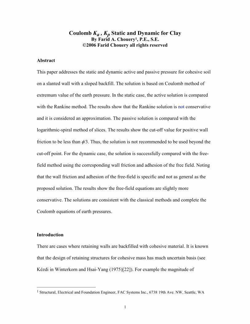
a) Active Condition

Consider Fig. 1 where the active force Eax is to be determined for a slanted wall with an

angle ξ, the slope of the top surface β, a surcharge q, and a critical height hc of the

cracked section.

cos coscos( )

α βξ β−

Lsin cos

cos( )ξ βξ β−

hc

q - Surcharge

x

z

β−ξ

β ξ

coscos( )

αξ β−

L

Lz

=+ −sin cos tan( )α α ξ β

ξ

δ

α

α−φ

φQ

cL

c'z

W

H

z

zc

T

c

h

h α+ξ−β

π/2+β−ξ

Eax

Eaz

ξ

FIG. 1 - Crossection Showing the Forces and the Geometry

4

If the wall height is H then the forces for the height h below hc are to be considered. The

total weight WT can be written as

WzL

qh L

hh L

T

c

c

c= ++

−

+

+

−

γ

αξ β α β

ξ βγ

ξ β α βξ β2

2

2cos

sin cos cos cos

cos( )

sin cos cos cos

cos( )....(1)

where

Lz

zh

h H hc=+ −

= = −−sin cos tan( ) cos

cos cos

cos( )α α ξ β ξξ βξ β

, , and ......................... (2)

Summing the forces in the x and z direction yields

E W Q cLax T= + − −sin sin( ) cosξ α φ α ........................................................................ (3)

E c z W Q cLaz T= − + − − −' cos cos( ) sinξ α φ α ............................................................. (4)

where c' is the adhesion and it has the same sign as the friction angle δ on the wall.

Eliminating Q from Eq. 3 and 4, substituting E Eaz ax= tanδ , L and z from Eq. 2, and WT

from Eq. 1 yields

Eh

f hg c c tax = + +γ

α φ β ξ δ γ α φ β ξ δ γ α φ β ξ2

2( , , , , ) ( , , , , , , ' ) ( , , , ) ..................................... (5)

where

[ ][ ]f ( , , , , )

sin cos tan( )

tan tan( ) tan tan( ) cosα φ β ξ δ

ξ ξ α φ

δ α φ α ξ β ξ=

+ −

+ − + −1 2 .................................... (6)

[ ][ ][ ]

g c cq

hc( , , , , , , ' )sin cos tan( ) cos

tan tan( ) tan tan( ) cos( ) cosα φ β ξ δ

ξ ξ α φ β

δ α φ α ξ β ξ β ξ γ=

+ −

+ − + − −+

1

[ ] [ ]

[ ][ ]−

− + + − + −

+ − + −

( / ) tan tan( ) ( ' / ) tan( ) tan tan( )

tan tan( ) tan tan( ) cos

c cγ α α φ γ α φ α ξ β

δ α φ α ξ β ξ

1

1 .............. (7)

[ ][ ]

tq h

hc

c( , , , )sin cos tan( ) cos sin

tan tan( ) cos( )α φ β ξ

ξ ξ α φ β ξ

δ α φ ξ β γ=

+ −

+ − −+

1 2 ......................................... (8)

5

The total vertical force is E E c zaz az= + ' where E Eaz ax= tanδ , and the resultant force is

E E Ea ax az= +2 2 . To maximize Ea it can be seen that Eax can be maximized instead.

Rewriting Eq. 5 as

Eh l m n

u v wax =

+ ++ +

γ α αα α

2 2

22

tan tan

tan tan ............................................................................ (9)

where

Aq

h

h

h

c= +−

+

1 22cos

cos

cos( ) cosξβ

ξ β ξ γ .................................................................. (10)

Bh

h

q

h

h

h

c c=−

+

sin cos

cos( )

ξ βξ β γ

2

............................................................................... (11)

lB c

h

c

h=

−− −

cos( )

cos cos

'

cos

ξ φφ γ ξ γ ξ

2 2 .......................................................................... (12)

[ ]m

A c

h

B=

−−

− −+

− −−

cos( )

cos

' tan( ) tan

cos

sin( )

cos cos( )

ξ φφ

ξ β φγ ξ

ξ β φφ ξ β

2 2 .................................... (13)

[ ]n

A B c

h

c

h=

+ − −− +

−tan( ) sin( )

cos cos

' tan tan( )

cos

ξ β ξ φφ γ ξ

φ ξ βγ ξ

2 2 ................................. (14)

u = +tan tanφ δ ......................................................................................................... (15)

v = + − + −(tan tan ) tan( ) tan tanφ δ ξ β φ δ1 ............................................................... (16)

w = − −( tan tan ) tan( )1 φ δ ξ β .................................................................................... (17)

6

Maximizing Eax with respect to α yields ∂∂α

∂ α∂α

∂∂ α

E Eax ax= =(tan )

(tan ).0 Thus, tanα can be

extracted from Eq. 9 as

baa −±−= 2tanα ................................................................................................. (18)

where

alw nu

lv mub

mw nv

lv mu=

−−

=−

− , and ............................................................................... (19)

Therefore, evaluate l, m, n, u, v and w from Eq. 12 to 17 and substitute in Eq. 19 and find

tanα from Eq. 18. Substitute tanα in Eq. 9 to find Eax maximum or evaluate α and

substitute in Eq. 5 to find Eax maximum. Hence, the Coulomb active condition is

obtained.

b) Passive Condition

To find the passive pressure Epx: set hc = 0, replace φ by -φ, c by -c, δ by -δ, and c' by -c'

in Eq. 12 to 17 and evaluate tanα and α from Eq. 18. Substitute tanα in Eq. 9 and obtain

Epx minimum the passive force normal to the wall. Alternatively, substitute α in the

following equation to obtain Epx to find the minimum:

Eh

f hg c cpx = − − + − − − −γ

α φ β ξ δ γ α φ β ξ δ2

2( , , , , ) ( , , , , , , ' ) ............................................. (20)

The total vertical force E pz , and the resultant Ep can be obtained from:

7

E E c z E E Epz px p pz px= + = +tan 'δ , and 2 2 .......................................................... (21)

Note: δ and c' are considered positive when the tangential force is downward on the wall.

This is consistent with standard practice for the passive condition. On the other hand, in

the active condition, δ and c' are considered positive when the tangential force is upward

on the wall.

c) Pressure Diagram

The active pressure distribution, σax, normal to the wall can be found by taking

σ∂∂

ξ∂∂ax

ax axE

z

E

h= = cos . Differentiating Eq. 5 yields

σ γ ξ γ ξ ξγ ∂

∂γ

∂∂

∂∂ax h f g

h f

hh

g

h

t

h= + + + +

( cos ) ( ) ( cos ) ( ) cos

( ) ( ) ( )

2

2 ..................... (22)

The right hand term in the brackets in Eq. 22 can be written as ∂α∂

∂∂αh

Eax , which is zero

since α is from Eq. 18. Thus, the active pressure normal to the wall becomes:

σ γ ξ α φ β ξ δ γ ξ α φ β ξ δax h f g c c= +( cos ) ( , , , , ) ( cos ) ( , , , , , , ' ) ........................................ (23)

The upward tangential shear on the wall becomes:

τ σ δaxz ax c= +tan ' .................................................................................................... (24)

Similarly, the passive pressure, σpx, normal to the wall becomes

8

σ γ ξ α φ β ξ δ γ ξ α φ β ξ δpx h f g c c= − − + − − − −( cos ) ( , , , , ) ( cos ) ( , , , , , , ' ) .............................. (25)

where hc = 0 in the g( ) function. The downward tangential shear on the wall becomes:

τ σ δpxz px c= +tan ' ..................................................................................................... (26)

d) Example (1)

(See example by Prabhakara (1965)[12]) Determine the active force against a vertical

wall 12m (39.37ft) in height with the following data available:

φ = 30 degrees δ = +20 degrees c = c' = 1250 kg/m2 (255.58 lb/ft2 )

ξ = β = 0 q = 0 γ = 1870 kg/m3 (116.66 1b/ft3 )

hc

h H hc c= + = = − = − =4

45 2 4 63 12 4 63 7 37γ

φtan( / ) . . . m (15.19 ft), m (24.18 ft)

Substituting in Eq. 10 through 19 yields (A = 2.257, B = 0, l = -0.363, m = 2.362, n =

-1.484, u = 0.941, v = 0.790, w = 0, a = -0.557, b = -0.467), tanα = 1.438, and α = 55.19

degrees. Substituting tanα = 1.438 in Eq. 9 yields E hax / ( . ) .05 0 37682γ = . Thus,

E E Eax az ax= = =19 129 6 962, tan , kg / m (12.84 kips / ft) , kg / m (4.67 kips / ft), δ

and E Eax az

2 2 20 356+ = , kg / m (13.67 kips / ft) . This number matches Prabhakara

within 1%, a slide rule error. However, E E c hza az= + =' ,16 173 kg / m (10.68 kips / ft) ,

and the actual resultant is E E Ea ax az= + =2 2 25 050, kg / m (16.82 kips / ft) .

9

e) Critical Height hc

If assuming ξ = 0, q = 0, δ = 0, and c' = 0, then h cc = +( / ) tan( / / )4 4 2γ π φ can be used

for a wall with a flat surface on top, and possibly for a semi-infinite soil with a sloped

surface on top with an angle β , see Terzaghi (1943)[20]. However, for other conditions,

hc will vary with many parameters besides c, γ, and φ. Additionally, based on an existing

crack intersecting the slip surface, Terzaghi (1943)[20] showed that the critical height can

be as low as h cc = +( . / ) tan( / / )2 67 4 2γ π φ . To find the exact hc : set hc = 0, δ = 0, and c'

= 0 in all the equations for the active condition, then solve for h that makes Eax = 0 in Eq.

5 or Eq. 9. This can be done by Newton Ralphson's iteration, the secant method, which

can be found in any numerical analysis textbook. Then h hc = −* cos( ) / (cos cos )ξ β β ξ

where h* is the root of the equation Eax = 0. Note: there exists a maximum of two roots.

One of the roots is h* = 0 and it is not desirable. The initial h value in the iteration should

be selected large enough to extract the desirable second root. Consequently, the

theoretical hc can be extracted. To obtain Terzaghi's reduction simply reduce hc by 2/3.

If σ ax in Eq. 23 is greater than zero at h = 0, then the iteration will converge to h* = 0 and

hc cannot be found. This situation will occur since σ γ α φ β ξax h g c(@ ) ( , , , , , , )= =0 0 0 and

it can take a positive value for some surcharge q.

f) Example (2)

Determine the active force against a slanted wall ξ = +5 degrees, 10 m (32.81 ft) high,

with a sloped backfill β = 20 degrees, for the available data

10

φ = 30 degrees q = 1140 kg/m2 (233.09 lb/ft2) c = 1250 kg/m2 (255.58 lb/ft2)

δ = 20 degrees c' = 1000 kg/m2 (204.5 lb/ft2) γ = 1870 kg/m3 (116.66 lb/ft3)

Use theoretical hc and compare with using h cc = + =( / ) tan( / ) .4 45 2 4 63γ φ m (15.19 ft) .

case (i): h cc = + =( / ) tan( / ) .4 45 2 4 63γ φ m (15.19 ft) :

Thus, h = 10 - 4.63(.969) = 5.512 m (18.08 ft). Substituting in Eq. 10 through 19 yields

(A = 2.865, B = 0.076, l = -0.359, m = 3.105, n = -1.662, u = 0.845, v = 0.619,

w = -0.226, a = -0.522, b = -0.114), tanα = 1.144, and α = 48.84 degrees. Substituting

tanα in Eq. 9 yields E hax / ( . ) .05 089432γ = . Thus, Eax = 25 403, kg / m (17.06 kips / ft) ,

E E c hza ax= + =tan ' ,δ 12 339 kg / m (8.29 kips / ft) , and the resultant is

E E Ea ax az= + =2 2 28 241, kg / m (18.96 kips / ft) .

case (ii) Theoretical hc :

Set hc = 0, δ = 0, and c' = 0 in all the equations and solve for h = h* = 2.8139 m (9.232 ft)

that makes Eax = 0. Thus, hc = 2.903 m (9.525 ft) with (A = 1.431, B = 0, l = -0.477, m =

1.497, n = -1.175, u = 0.577, v = 0.845, w = -0.268, a = -0.636, b = -0.467, tanα = 1.57,

and α = 57.5 degrees) making Eax = 0. By using hc = 2.903 m (9.525 ft), and

h = 10 - 2.903(.969) = 7.186 m (23.58 ft), substituting in Eq. 10 through 19 yields (A =

1.962, B = 0.02, l = -0.316, m = 2.165, n = -1.165, u = 0.845, v = 0.619,

w = -0.226, a = -0.522, b = -0.114), tanα = 1.143, and α = 48.81 degrees. Substituting

tanα in Eq. 9 yields E hax / ( . ) .05 056602γ = . Thus, Eax = 27 331, kg / m (18.35 kips / ft) ,

11

E E c hza ax= + =tan ' ,δ 14 537 kg / m (9.76 kips / ft) , and the resultant is

E E Ea ax az= + =2 2 30 957, kg / m (20.79 kips / ft) .

Hence, the increase in the resultant due to the difference in the critical height hc in case (i)

and (ii) is 9.62% which is considerable due to the surcharge.

g) Comparison of Coulomb Equations with Rankine Equations

Historically, Rankine's (1857)[14] solution for cohesion is popular since it is very easy to

do a graphical method on a Mohr diagram (see Terzaghi (1943)[20] and Kézdi in

Winterkorn and Hsai-Yang (1975)[22]). On the other hand, Coulomb method required

several trial surfaces before reaching the optimal forces. For a semi-infinite mass with a

plane surface at an angle β to the horizontal and with vertical wall (ξ = 0), similarly the

Rankine stress can be written as (formula revised)

zcbaz

cax γγφ

γφβ

βσ

++−

++−= 0002

22 2tan2

cos

cos21cosRankine)( .................. (27)

where

24

0

2

02

2

0 cos

cos

cos

cos and ,

cos

costan

2 ,

cos

1

−

=

=

=

φβ

φβ

φβ

φγφγ

cz

cb

z

ca

When allowing tension (hc = 0), the active resultant force can be expressed as

E dza ax

h

= ∫σ0

and has a directional angle β . Note: in Rankine method the friction and the

adhesion on the wall do not enter the equation (Eq. 27). Thus, the Rankine method is

12

considered an approximation. One major difference between the Rankine and the

Coulomb method for cohesion is that with the Rankine method the directional angle of

the resultant is constant and is equal to β . On the other hand, with the Coulomb method

the directional angle varies with depth when there is adhesion. The shear due to the

adhesion on the wall increases with depth but the directional angle

[ ] )//()/'(tan 2zEzc ax γγδ + decreases. At z → ∞ the directional angle becomes δ. Since

the adhesion and the friction on the wall are essential parameters, then it is clear that the

Coulomb equation is more accurate than the Rankine equation. The results show that the

Rankine equation seems to be not conservative. Even when setting c' = 0, one finds the

equations do not match. For example if set c' = 0, δ = β = φ = 30 degrees, hc = q = 0, and

c/(γz) = 0.1, then )5.0/( 2hEa γ = 0.3317 for Coulomb and )5.0/( 2hEa γ = 0.2983 for

Rankine, a difference of 11.2 %. Note: in the case of granular material the equations

match when δ = β with ξ = 0. Also, in the case of granular material the Rankine equation

has been used as an approximation (see Das (1994)[4]).

h) Comparison of Coulomb Passive Pressure with Log-Spiral Method of Slices

Shields and Tolunay (1973)[19] did a modified Terzaghi (1943)[20] analysis for passive

pressure in granular material on a wall with positive friction. In their solution they used

the method of slices and assumed the vertical shear to be zero on each slice except for the

first slice next to the wall. The slip surface they used is a logarithmic spiral and their

results were close to experimental findings. Basudhar and Madhav (1980)[1] repeated the

analysis and included cohesion and pore pressure. In their analysis they did not use the

13

same initial angle2 αw at the wall between the logarithmic spiral and the horizontal.

Instead, they optimized the function with respect to the center of the logarithmic spiral. In

many ways the optimization could also have been done with respect to αw instead of the

center of the logarithmic spiral. Rewriting the logarithmic spiral equations to include the

surcharge q with hc = 0, the slice horizontal force can be found from Eq. 5, yielding

dE zdz f dz g cpx = − + − −( ) ( , , , , ) ( ) ( , , , , , , )γ α φ γ α φ0 0 0 0 0 0 0 ............................................... (28)

where

z z r e w= + + −0 0 cos( ) tan ( )α φ φ α α ..................................................................................... (29)

dz r d e w= −0 α α φ φ α αsin sec tan ( ) ...................................................................................... (30)

z r w0 0= − +tan sin( )ψ φ α .......................................................................................... (31)

r h w0 = + +cos sec( )ψ ψ φ α ....................................................................................... (32)

ψ π φ= −/ /4 2 ......................................................................................................... (33)

f ( , , , , ) tan( ) cotα φ α φ α− = +0 0 0 ................................................................................ (34)

[ ]g c q c( , , , , , , ) ( / ) tan( ) cot ( / ) tan tan( ) cotα φ γ α φ α γ α α φ α− − = + + + +0 0 0 0 1 ........... (35)

and α is the slice wedge angle with the horizontal. Summing all the horizontal forces of

all the slices except for the slice next to the wall, yields

dE zdz

df

dz

dg d

re

r zq

e rq c

e d

pxw

w w

= +

= +

− +

+ +

+

+

−

− −

∫∫

∫

γα

γα

α γ α φ

γγ

α φ γγ

φγ

α φ α

φ α α

φ α α φ α α

( ( sin ( )

cos( ) tan sec( )

tan ( )

tan ( ) tan ( )

) )

+ z0

02

2 2

0 0 0

2

.................................................................. (36)

2 In a later article by the author 2007 titled “Kp for a Wall with Friction with Exact Slip Surface” the initial angle αw by Shields and Tolunay (1973)[19] is correct.

14

where the integral dE px∫ in Eq. 36 needs to be evaluated from αw to ψ. Thus, the passive

force can be expressed as

EP dE c h

px

R px w

w

w=+ + +

− +

∫ ' tan( )

tan tan( )

α φ

δ α φα

ψ

1 .......................................................................... (37)

where

P h qh chR = +

+ + +γ

π φ π φ2

4 2 2 4 202

02

0tan ( / / ) tan( / / ) ...................................... (38)

and h z r e w

0 0 0= + −sin tan ( )ψ φ ψ α . Hence, for a given h pick αw and find r0 and z0 from Eq.

32 and 31, evaluate the integral dE px∫ from Eq. 36 from α = αw to α = ψ and integrate

numerically the last term in the equation, then evaluate PR from Eq. 38 and substitute in

Eq. 37 to evaluate E px for a given positive δ and c'. Repeat the process with different αw

until E px minimum is found.

For granular soil with q = c = c' = 0 the results match Basudhar and Madhav (1980)[1].

Also, the results match Shields and Tolunay (1973)[19] if

[ ]{ }α φ δ φ δ φ φ δw = − − − − −05. arccos cos( ) sin( ) cot where δ takes a positive value.

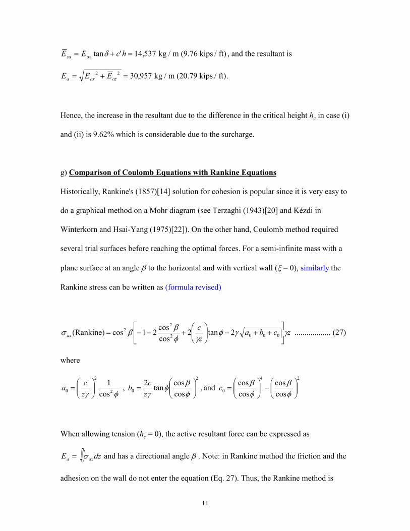
Comparing Eq. 37 with Coulomb Eq. 20 with ξ = β = 0, yields the curves in Fig. 2 where

2 2E hpx / ( )γ is plotted against δ for ρ γ γ= = =c h c h' /( ) / ( ) ,0 0.1, and 0.2, φ = 30

degrees, and q = 0. Note: for δ > φ/3 the difference is very large. However, for δ φ≤ / 3

15

the Coulomb method and the logarithmic spiral method of slices are close, within 11% at

maximum point. This is a reasonable cut-off point for the Coulomb equation. Terzaghi

(1943)[20] recommended δ φ≤ / 3 be used for computing the passive pressure by means

of Coulomb's equation for granular soil. This is also the author's recommendation for

cohesive soil. This is necessary since both methods have been traditionally used.

0 5 10 15 20 25 30 352

4

6

8

10

12

14

16

Angle of Friction δ

22

E

h

px

γ

Coulomb MethodLog-spiral Method

ρ=0.1

ρ=0.2

ρ=0

ρ=0.2

ρ=0.1

ρ=0

ργ γ

= =c

h

c

h

'

FIG. 2 - Passive Pressure Coefficient with Cohesion

CASE II: DYNAMIC CONDITION

Since Mononobe and Okabe (1929 & 1924)[8,11] developed a method, by modifying

Coulomb's solution, to evaluate dynamic earth pressures against retaining structures, a

number of studies have been performed on this subject in granular soil, but not many in

cohesive soil. Prakash and Saran (1966)[13] derived an equation for dynamic active

cohesive soil pressure against retaining structure on the assumptions mostly employed by

16

Mononobe-Okabe. They adapted the pseudo-static approach in considering the dynamic

effect of the backfill soil where they included the contributions of soil cohesion and

uniform backfill surcharge to the dynamic lateral pressure. An allowance for tension

cracks due to cohesion was also made. Since the Coulomb equation Eq. 5 is now

complete and has the effect of slop backfill (β angle), the full dynamic range can be

employed instead of the pseudo-static approach.

a) Active Condition

Following Mononobe and Okabe (1929 & 1924)[8,11], replace H by H sec cos( )ξ ξ θ+ , h

by H hcsec cos( ) sec( ) cos( ) cos( )ξ ξ θ ξ β ξ θ β θ+ − − + + , γ by γ θ( ) sec1− kv , ξ by ξ + θ,

and β by β + θ in Eq. 10 through 17, where [ ]θ = −arctan / ( )k kh v1 , kh and kv are the

horizontal and vertical acceleration coefficients. Thus, by substituting in Eq. 18 to find

tanα, then in Eq. 9, Eax can be found. This simple procedure yields the seismic resultant

active force EaE and its directional angle δE to be

E E E c zaE ax ax= + +2 2( tan ' )δ ............................................................................... (39)

δδ

E

ax

ax

E c z

E=

+tan ' .................................................................................................. (40)

Often the interest is in the horizontal component of the resultant force. The horizontal

component can be written as:

17

E EaE aE E, cos( )h = +δ ξ .............................................................................................. (41)

Note: hc needs to be evaluated independently as described in section e) in the CASE I-

Static Condition. If the soil can take tension then hc = 0.

b) Passive Condition

Following Mononobe and Okabe (1929 & 1924)[8,11], replace h by h sec cos( )ξ ξ θ+ , γ

by γ θ( ) sec1− kv , ξ by ξ − θ, β by β − θ, φ by −φ, δ by −δ, c' by −c', and set hc = 0 in Eq.

10 through 17. By substituting in Eq. 18 to find tanα, then in Eq. 9, Epx can be found.

This simple procedure yields the seismic resultant passive force EpE and its directional

angle δE to be

E E E c zpE px px= + +2 2( tan ' )δ .............................................................................. (42)

δδ

E

px

px

E c z

E=

+tan ' ................................................................................................... (43)

The horizontal component can be written as:

E EpE pE E, cos( )h = +δ ξ ............................................................................................. (44)

Note: the solution is valid only for δ φ≤ / 3 as was pointed out in the static case.

c) Comparison with Recent Method

18

Richards and Shi (1994)[18] derived an elasto-plastic free field solution for earthquakes

acting on cohesive soil which they applied the solution directly to retaining structures. For

granular soil prior work in elasto-plastic was performed by Richards et al. (1990)[17].

One major difference between applying their method and the Mononobe-Okabe method

proposed in this paper (Eq. 39 and 42) is when θ = 0, the static condition, in their solution

the stresses are assumed linear and the shear is zero at the wall. This assumption was

necessary in their solution using the elasto-plastic fluidization of soil. However, for a wall

to develop no shear at θ = 0 is not likely and is apparent in the Coulomb method.

Furthermore, the pressure can be nonlinear per Eq. 23 and 25. This makes the Mononobe-

Okabe method proposed in this paper more applicable. However, the simple free-field

solution, will give the correct stresses on a retaining wall if it deforms exactly as dictated

by the free-field thereby maintaining the correct interface boundary condition. In order to

compare Eq. 39 with Richards and Shi (1994)[18] equations, the friction and the adhesion

on the wall must correspond to their assumption. For granular soil they showed that tanδ

must equal tan /θ K AE in order to match Mononobe-Okabe method, where KAE is from

their paper. Similarly, for cohesive soil it is necessary to set the adhesion c' = 0, to allow δ

to be greater than φ , and use

tanδ =T

N

AE

AE

.............................................................................................................. (45)

where TAE and NAE are from Richards and Shi's paper. Setting, kv = 0, c' = 0, q = 0, φ = 30

degrees, hc = 0, and ξ = β = 0 in all the equations that lead to Eq. 39, and plotting the

normalized seismic resultant active force 2 2E haE / ( )γ versus kh for both methods using

ρ = c/γh = 0, 0.05, and 0.1 yields the curves in Fig. 3. The results show the free-field

19

solution is more conservative than the Mononobe-Okabe solution: about 19% increase at

the worst point on Fig. 3.

For the passive pressure, replace TAE and NAE in Eq. 45 by TPE and NPE from Richards and

Shi's paper. Setting, kv = 0, c' = 0, q = 0, φ = 30 degrees, ξ = β = 0, and all the passive and

FIG. 3 - Comparison of Free Field and Mononobe-Okabe's Method for Active Thrust

for Case with Tension Allowed (hc = 0)

0 0.1 0.2 0.3 0.4 0.5 0.6 0.7 0.80

0.5

1

1.5

2

22

E

h

aE

γ

kh

Free Field

Mononobe-Okabe

ργ

=c

h

ρ = 0.1

ρ = 0.05ρ = 0, φ = 30

ο

20

0 0.1 0.2 0.3 0.4 0.5 0.6 0.7 0.82

2.5

3

3.5

4

ργ

=c

h

22

E

h

pE

γ

kh

ρ = 0

ρ = 0.1

Free FieldMononobe-Okabe

, φ = 30ο

FIG. 4 - Comparison of Free Field and Mononobe-Okabe's Method for Passive Thrust

seismic requirements in all the equations that lead to Eq. 42, and plotting the normalized

seismic resultant passive force 2 2E hpE / ( )γ versus kh for both methods using ρ = c/γh =

0, and 0.1 yields the curves in Fig. 4. The results show the free-field solution is slightly

more conservative than the Mononobe-Okabe solution: about 3% decrease at the worst

point on Fig. 4.

d) Design Criteria

Even in moderate earthquakes, gravity walls without lateral bracing slide at their base

(Richards and Elms (1979)[16]). For cohesionless soil the total thrust for different wall

movement has been traditionally calculated using Mononobe-Okabe's equation. Also, the

total thrust is almost the same as that calculated by free-field analysis (Richards

21

(1991)[15]) and can also be used for β = ξ = 0. Similarly, for cohesive soil, the thrust

calculation can be used from the Mononobe-Okabe Eq. 39 as well from the free-field

equation of Richards and Shi for β = ξ = 0. Thus, for sliding failure, the straightforward

method presented by Richards and Elms (1979) [16] for cohesionless soil and Richards

and Shi (1994)[18] for cohesive soil can be extended for limit analysis and design with

cohesive soil that includes β and ξ slope angle configurations. The extended analysis

yields

[ ]W

E c B

kw

aE E b E w

v b

=+ − + −

− −

cos( ) tan sin( ) "

( )(tan tan )

δ ξ φ δ ξ

φ θ1 .................................................... (46)

where Ww is the self-weight of the retaining wall, EaE and δE are from Eq. 39 and 40, φb is

the friction angle between the soil and the bottom of the wall, Bw is the base dimension of

the wall, and c" is the adhesion on the base. When using Eq. 46 to map the ratio of the Ww

over the static weight verses kh (for kv = 0), the results show that the seismic

magnification for cohesive soil is even more dramatic than sand. This has been pointed

out by Richards and Shi (1994)[18]. Thus, for a given safety factor or weight to static

weight ratio the critical acceleration value kh* can be determined for a particular wall

using Eq. 46. Consequently, the seismic displacement for design can be obtained and

controlled by using Newmark's (1965) [10] sliding-block approach developed by

Richards and Elms (1979) [16] for walls. The incremental accumulation of displacement

can also be calculated by a more sophisticated method (Nadim and Whitman (1983) [9])

that is less conservative. Conversely, the wall can be designed to limit seismic

22

deformation to a tolerable value for the earthquake intensity specified by (Elms &

Richards (1979) [5]; Whitman and Liao (1985) [21]) as recommended by AASHTO

("Foundation" (1992) [6]).

Summary and Conclusions

The static Coulomb equations for a slanted wall with sloped backfill in cohesive soil are

finally completed in this paper. Furthermore, the solution is extended to derive the

dynamic earth pressure for cohesive soil per Mononobe-Okabe. The static active

Coulomb equation is obtained and is expected to give realistic forces and pressure on a

retaining wall in cohesive soil. Also, the active solution is compared with the Rankine

method. The results show that the Rankine solution is not conservative and it is

considered an approximation. As expected, the Coulomb passive equation is not adequate

for δ > φ/3 and the logarithmic-spiral method of slices is recommended as it was the case

for cohesionless soil. The earthquake solution is obtained and compared with the free-

field solution. In order to compare, the friction and the adhesion on the wall was made to

correspond to the free-field assumption. Noting that the proposed solution in this paper is

of more general application than the free-field solution. The results show that the free-

field solution is slightly more conservative than the Mononobe-Okabe equations

presented in the paper. The proposed general solutions are consistent with the classical

methods and complete the Coulomb equations of earth pressures.

23

Acknowledgments

The writer is deeply appreciative to his wife Bernice J.F. Chouery for the love and

patience in giving valuable family support to do this manuscript. Also, he is thankful to

the assistance provided by Shirley A. Egerdahl in proofreading this manuscript.

Appendix I.-References

1. Basudhar, P. K., and Madhav, M. R. (1980). "Simplified Passive Earth Pressure

Analysis," Journal of the Geotechnical Engineering Division, ASCE, Vol. 106, No.

GT4, pp. 470-474.

2. Coulomb, Charles Augustin (1776). "Essai sur une application des règles de maximis et

minimis à quelques problèmes de statique relatifs à l'architecture," Mem. Div. Savants,

Acad. Sci., Paris, Vol. 7.

3. Culmann, C. (1866), Graphische Statik, Zürich.

4. Das, B. M. (1994). Principles of Geotechnical Engineering, PWS Publishing Company,

Boston, Massachusetts, Chapter 10, pp. 421-423.

5. Elms, D. G., and Richards, R. (1979). "Seismic Design of Gravity Retaining Walls,"

Bull. of the New Zealand Nat. Soc. for Earthquake Engrg., 12(2), pp. 114-121.

24

6. "Foundation and Abutment Design Requirements," (1992). Division I-A− seismic design

commentary, sec. 6. American Association of State Highway and Transportation

Officials (AASHTO), pp. 393-400.

7. Mohr, O. (1871). "Beiträge zur Theorie des Erddruckes," Z. Arch. u. Ing. Ver.

Hannover, Vol. 17 (1871), p. 344, and Vol. 18 (1872), pp. 67, 245.

8. Mononobe, N. (1929). "Earthquake-Proof Construction of Masonry Dams," Proceedings

of the world Engineering Conference, Vol. 9, p. 275.

9. Nadim, F., and Whitman, R. V. (1983). "Seismically Induced Movement of Retaining

Walls," J. Geotech. Engrg., ASCE, 109(7), pp. 915-931.

10. Newmark, N. M. (1965). "Effects of Earthquakes on Dams and Embankments,"

Géotechnique, London, England, 15(2), pp. 139-160.

11. Okabe, S. (1924). "General Theory of Earth Pressure," Journal of Japanese Society of

Civil Engineers, Tokyo, Japan, Vol. 12, No. 1.

12. Prabhakara, K. S. (1965). "Analysis of Active Earth Pressure by Dimensionless

Parameters, " Journal of India National Society of Soil Mechanics and Foundation

Engineering, April 1965, Vol. 4, No. 2, pp. 197-206.

13. Prakash, S., and Saran, S. (1966). "Static and Dynamic Earth Pressures Behind

Retaining Walls," Proc. Third Symposium on Earthquake Engrg. Roorkee, India, pp.

277-288.

14. Rankine, W. J. M. (1857). "On the stability of loose earth," Trans. Royal Soc., London,

147.

25

15. Richards, R. (1991). "Dynamic Earth Pressure and Seismic Design of Earth Retaining

Structures," Proc., 2nd Int. Conf. on Recent Adv. in Geotech. Earthquake Engrg. and

Soil Dynamic, Vol. 3, General Rep. no. IV, St. Louis, Mo., pp. 2033-2038.

16. Richards, R., and Elms, D. G. (1979). "Seismic Behavior of Gravity Retaining Walls,"

Journal of the Geotechnical Engineering Division, ASCE, Vol. 105, No. GT4, pp. 449-

464.

17. Richards, R., Elms, D. G., and Budhu, M. (1990). "Dynamic Fluidization of Soils," J.

Geotech. Engrg., ASCE, 116(5), pp. 740-759.

18. Richards, R., and Shi, X. (1994). "Seismic Lateral Pressure in Soils with Cohesion," J.

Geotech. Engrg., ASCE, 120(7), pp. 1230-1251

19. Shields, D. H., and Tolunay, A. Z., (1973). "Passive Pressure Coefficients by Method of

Slices," Journal of the Soil Mechanics and Foundations Division, ASCE, Vol. 99, No.

SM12, Proc. Paper 10221, pp. 1043-1053.

20. Terzaghi, Karl (1943). Theoretical Soil Mechanics, Wiley and Sons, New York, pp. 39,

pp. 152-155, pp. 38-41, pp. 113-117, and pp. 107.

21. Whitman, R. V., and Liao, S. (1985). "Seismic Design of Gravity Retaining Walls,"

Misc. Paper GL-85-1, U.S. Army Corp of Engineering, Vicksburg, Miss.

22. Winterkorn, H. F., and Hsai-Yang, F. (1975). Foundation Engineering Hanbook, Van

Nostrand Reinhold Co., New York, N. Y., Chapter 5, by Á. Kézdi, pp. 209-211, and pp.

200-203.

26

Appendix II.- Notation

The following symbols are used in this paper:

α = wedge angle between a line parallel to the x-axis and the slip surface;

β = slope angle of backfill between the top surface and the horizontal line;

Bw = the base dimension of the wall;

c = soil cohesion;

c' = adhesion on the wall;

c" = adhesion between the wall base and soil;

δ = friction angle between back face of wall and soil;

δE = direction angle of seismic force of the wall;

Ea = resultant active force on the wall;

EaE = seismic active resultant force;

Eax = active force normal to the wall;

Eaz = active force tangent to the wall;

Eaz = active force tangent to the wall including wall adhesion;

Ep = resultant passive force on the wall;

EpE = seismic passive resultant force;

Epx = passive force normal to the wall;

E pz = passive force tangent to the wall including wall adhesion;

φ = angle of internal friction of soil;

φb = friction angle between the soil and the bottom of the wall;

hc = critical height zone of tension cracks;

27

q = surcharge load;

σax = active pressure normal to the wall;

σpx = passive pressure normal to the wall;

τaxz = active pressure tangent to the wall including wall adhesion;

τpxz = passive pressure tangent to the wall including wall adhesion;

Ww = the self weight of the retaining wall, and

ξ = slanted angle between the vertical line and the wall.