Embed Size (px)
Citation preview

Could the boom-bust in the eurozone periphery have
been prevented? ∗
Marcin Bielecki† Micha l Brzoza-Brzezina‡ Marcin Kolasa§
Krzysztof Makarski¶
Abstract
Boom-bust cycles in the eurozone periphery almost toppled the common currency and
recent experience suggests that they may return soon. We check whether monetary or
macroprudential policy could have prevented the periphery’s violent boom and bust
after the euro adoption. We estimate a DSGE model for the two euro area regions, core
and periphery, and conduct a series of historical counterfactual experiments in which
monetary and macroprudential policy follow optimized rules that use area-wide welfare
as the criterion. We show that common monetary policy could have better stabilized
output in both regions, but not the housing market or the periphery’s trade balance. In
contrast, region-specific macroprudential policy could have substantially smoothed the
credit cycle in the periphery and reduced the build-up of external imbalances. The best
outcome is achieved by coordinated monetary and macroprudential policies, though the
improvement over optimized macroprudential policy is not large.
JEL: E32, E44, E58
Keywords: euro-area imbalances, monetary policy, macroprudential policy, Bayesian
estimation
∗The views expressed herein are those of the authors and not necessarily those of Narodowy Bank Polski.We would like to thank the participants of the NBP-NBU conference in Kyiv, Computing in Economicsand Finance conference in Bordeaux, Dynare conference in Rome, European Economic Association AnnualMeeting in Geneva, NBP-Deutsche Bundesbank Workshop in Krakow, Schumpeter Seminar at the HumboldtUniversity in Berlin and seminar at DG-ECFIN in Brussels for useful comments.†Narodowy Bank Polski and University of Warsaw; Email: [email protected].‡Narodowy Bank Polski and Warsaw School of Economics; Email: [email protected].§Narodowy Bank Polski and Warsaw School of Economics; Email: [email protected].¶Narodowy Bank Polski and Warsaw School of Economics; Email: [email protected].
1

1 Introduction
The boom and bust cycle in the peripheral economies of the euro area is one of the most
dramatic (but also most interesting) experiences in the recent economic history of developed
countries. It started relatively innocently in the form of increasing demand and inflation
pressure in selected countries of the common currency area. Over time, however, it evolved
into a fully-fledged boom in the housing market, drew current accounts and international
investment positions into deeply negative territories and, after property markets collapsed,
triggered an economic, banking and fiscal crisis that almost toppled the common currency.
This episode has been extensively described in the literature (see e.g. Blanchard and
Giavazzi 2002; Brzoza-Brzezina 2005; Honohan and Leddin 2006; Blanchard 2007; Fagan
and Gaspar 2007; in’t Veld et al. 2012; Rabanal and Sanjani 2015). We summarize it briefly
in Figure 1, which plots the time series of output, net exports, housing loans and house prices
in the core (Austria, Belgium, Finland, France, Germany, Italy, Luxembourg, Netherlands)
and periphery (Greece, Ireland, Portugal and Spain) of the euro area. It is clear that the
boom-bust cycle was restricted to the latter region and was particularly stark in the housing
market. Our main goal is to check whether policy, be it monetary or macroprudential, could
have prevented such a scenario.
We do not build on empty ground. The existing literature has already pointed to macro-
prudential policy as a possible solution to the problem of asymmetries in a monetary union.
Obviously, common monetary policy cannot deal with asymmetric shocks, especially if they
affect a relatively small part of the common currency area (the GDP share of the affected
peripheral members only slightly exceeds 15%). However, a properly designed macropru-
dential policy could in principle complement monetary policy, as long as the asymmetric
developments show up in areas where such policy can be effective. Since the boom-bust
in the eurozone periphery was largely concentrated in the residential property market, the
literature has mainly focused on the potential gains that can be achieved with adjustments
in the macroprudential policy instruments related to housing mortgages.
Quint and Rabanal (2014) study the optimal mix of monetary and macroprudential poli-
cies in the euro area and find that the introduction of a rule affecting credit spreads would help
in reducing macroeconomic volatility and hence in improving EMU-wide welfare. Brzoza-
Brzezina et al. (2015) conclude that macroprudential policy using the loan-to-value (LTV)
ratio as an instrument can substantially improve welfare in the euro area member countries
affected by asymmetric shocks, provided that it is implemented at a national rather than
union-wide basis. Rubio (2014) develops this finding further and shows that the outcomes
depend on the source of the observed heterogeneity between the member states, with po-
tential welfare gains achievable when the asymmetries originate in the housing market. Our
paper is also related to the vast literature that asseses macroprudential policy without ex-
2

plicitly modeling a monetary union (see e.g. Darracq-Paries et al. (2011); Lambertini et al.
(2013); Claessens (2014)).
While all these papers show a clear direction for future policies, they do not necessarily
give a clear answer to the question stated in this paper’s title. This is because their con-
clusions are based on stochastic simulations applied to a typical business cycle environment.
However, as we confirm in our analysis, the series of shocks that hit the eurozone periphery
was quite special in terms of sign and size. For this reason, we focus on the particular period
when the boom developed and then turned into bust. Our results are thus based on his-
torical counterfactual simulations for the period since the eurozone was created. Moreover,
while designing such experiments it is crucial to account for potential structural heterogene-
ity between the core and peripheral countries as this may lead to different responses of key
macroaggregates even in response to common shocks. Therefore, we base our conclusions
on an estimated model where the two regions of the euro area are not only hit by asym-
metric shocks, but also are allowed to differ in average leverage as well as nominal and real
rigidities. Indeed, we find that these structural differences make the periphery more prone
to boom-bust cycles originating in the housing market.
Given the pronounced role of the housing market in the recent eurozone crisis, and our
focus on counterfactual simulations with alternative monetary and macroprudential policy
adjustments, our modeling strategy is relatively clear-cut. We construct a New Keynesian
two-region DSGE model featuring a housing market, real and nominal frictions, and common
monetary policy. The model is then estimated using macroeconomic data for the two areas
of the eurozone. Our estimation confirms a pronounced role of housing markets in driving
the boom in the periphery and its larger vulnerability.
Next, we conduct a series of counterfactual simulations. Our evaluation is based on
social welfare function. We begin by checking whether common monetary policy could have
prevented the boom-bust. To this end we generate counterfactual scenarios with monetary
policy rule parameters optimized such that area-wide welfare in stochastic equilibrium is
maximized. We show that such policy could have stabilized output in both regions of the
monetary union quite well. However, its ability to affect housing loans or the trade balance
is very limited. In contrast, macroprudential policy could have significantly smoothed the
credit cycle in the periphery. It also appears as a promising way of limiting the build-up
of external imbalances in this relatively more vulnerable region. Best results are achieved
by co-ordinated monetary and macroprudential policies. Such policy smoothes both output
and credit and improves welfare.
The rest of the paper is structured as follows. In Section 2 we present the model, and in
Section 3 we document its estimation and stochastic properties. Section 4 presents historical
shock decompositions and discusses how differences in the economic structure make the
periphery more prone to boom-bust cycles. In section 5 we describe the counterfactual
3

simulations. Section 6 concludes.
2 Model
We construct a two-region DSGE framework with collateral constraints modeled as in Ia-
coviello (2005). These two regions, called core and periphery, form a monetary union. Mea-
sure ω of agents reside in the periphery and ω∗ = 1 − ω in the core. Both economies are
populated by patient households (who save in equilibrium) and impatient households (who
borrow in equilibrium), as well as producers of final goods, housing and intermediate goods.
Union-wide monetary policy is conducted according to a Taylor rule, while macroprudential
policy instruments can be adjusted at the regional level.
In what follows, variables and parameters without an asterisk refer to the periphery,
while those with an asterisk refer to the core. Variables without time subscripts denote their
respective steady state values. Since both regions have a symmetric structure, we describe
the problems of agents in the periphery only.
2.1 Households
In each economy there are two types of households indexed by ι on a unit interval: patient
ι ∈ P ≡ [0, ωP ] and impatient ι ∈ I ≡ (ωP , 1].1 Hence, the measure of patient agents is ωP ,
while that of impatient households is ωI = 1− ωP .
2.1.1 Patient households
Patient households discount the future with factor βP and optimize by choosing consumption
cP,t, housing services χP,t and labor supply nP,t. They set their own nominal wages WP,t in
a monopolistically competitive environment and deposit savings DP,t in the banking sector,
repaid with interest rate Rt known in advance. We assume that patient households own all
capital, as well as all shares of firms and banks in the economy. Thus, they receive rent Rk,t
from owned capital2 kP and dividends ΠP,t. They also pay two lump sum taxes, one as a
fixed redistributive transfer to impatient households τP and the other to finance government
consumption τt.
A ι-th representative patient household maximizes its expected utility
1We employ the following notational convention: all variables denoted with a subscript P or I are ex-pressed per patient or impatient household, respectively, while all other variables are expressed per allhouseholds. For example, k denotes per capita capital and since only patient households own capital, capitalper patient households is equal to kP = k/ωP .
2We assume that the capital stock is fixed at the aggregate level.
4

UP,t = E0
{ ∞∑t=0
βtP
[εu,t
(cP,t (ι)− ξccP,t−1)1−σc
1− σc
+ εu,tεχ,tAχν(χP,t)− AnnP,t (ι)1+σn
1 + σn
]}, (1)
subject to the budget constraint
PtcP,t (ι) + Pχ,t [χP,t (ι)− (1− δχ)χP,t−1 (ι)] +DP,t (ι) + τP + τt
≤ WP,t (ι)nP,t (ι) +Rk,tkP (ι) +Rt−1DP,t−1 (ι) +ΠP,t (ι), (2)
where ξc measures the degree of external habit persistence in consumption, Aχ and An are
the weights of housing and labor in utility, σc denotes the inverse of intertemporal elasticity
of substitution in consumption, σn is the inverse Frisch elasticity of labor supply, and δχ
is the rate of housing depreciation. There are two preference shocks – an intertemporal
preference shock εu,t and a housing preference shock εχ,t, both following independent AR(1)
processes. Finally, prices of consumption and housing are denoted as Pt and Pχ,t. In what
follows, prices written with lower case letters are expressed in real terms, relative to the CPI
index Pt.
While estimating and simulating the model, following Justiniano et al. (2015) we assume
that the utility of the housing services flow ν(χP,t) is such that it implies a rigid housing
demand of patient households at the level χP . This assumption implies that there is no
reallocation of houses across the two types of households, which can be motivated by some
housing market segmentation, as argued by Landvoigt et al. (2015). It is also consistent with
the argument by Geanakoplos (2010) that prices are determined by marginal agents.
2.1.2 Impatient households
Impatient households discount the future with factor βI < βP and optimize by choosing
consumption cI,t, housing services χI,t and labor supply nI,t. They set their nominal wages
WI,t and acquire loans LI,t from the banking sector, charged with interest rate RL,t known
in advance. Access to credit is constrained by the value of collateral. While impatient
households pay a tax financing government spending just as patient households, they also
receive a redistributive lump sum transfer τI .
A ι-th representative impatient household maximizes its expected utility
5
UI,t = E0
{ ∞∑t=0
βtI
[εu,t
(cI,t (ι)− ξccI,t−1)1−σc
1− σc
+ εu,tεχ,tAχ(χI,t (ι)− ξχχI,t−1)1−σχ
1− σχ− An
nI,t (ι)1+σn
1 + σn
]}, (3)
where ξχ and σχ denote the degree of external habit persistence and the inverse of intertem-
poral elasticity of substitution in housing, respectively. This optimization is subject to the
budget constraint
PtcI,t (ι) + Pχ,t [χI,t (ι)− (1− δχ)χI,t−1 (ι)] +RL,t−1LI,t−1 (ι) + τt
≤ WI,t (ι)nI,t (ι) + LI,t (ι) + τI (4)
and the collateral constraint on credit
RL,tLI,t (ι) ≤ mχ,tEt {Pχ,t+1} (1− δχ)χI,t (ι) , (5)
where mχ,t is the LTV ratio set by the macroprudential authority.
2.1.3 Labor market
The differentiated labor services of patient and impatient households are purchased by com-
petitive aggregators who transform them to standardized labor services nt using the following
technology
nt =
[ω
1φn
P nφn−1φn
P,t + ωI1φn n
φn−1φn
I,t
] φnφn−1
, (6)
where
nP,t =
[1
ωP
ˆ ωP
0
nP,t (ι)1µw dι
]µwand nI,t =
[1
ωI
ˆ ωI
0
nI,t (ι)1µw dι
]µw. (7)
In the formulas above, φn measures the elasticity of substitution between patient and impa-
tient labor, and µw denotes households’ markup over the competitive wage level.
Nominal wages set by the households are sticky as in the Calvo scheme, and within each
period only a fraction 1 − θw of them receives a signal to reoptimize. Others update their
wages according to πζw,t = ζwπt−1 + (1− ζw) π, where πt ≡ Pt/Pt−1 is CPI inflation, π is its
steady state level, and ζw is the weight of past inflation in the wage indexing scheme. We
assume that households share risk perfectly within each type, either through large families
6

or through access to complete markets for Arrow-Debreu securities. Thus, wage stickiness
does not translate into consumption and housing stock heterogeneity.
2.2 Producers
There are three types of producers in the economy – final goods, housing and intermediate
goods producers. All of them are owned by patient households. The first two types of pro-
ducers operate in perfectly competitive markets and use only intermediate goods as inputs,
which in turn are produced by monopolistically competitive sector that employs capital and
labor.
2.2.1 Final goods producers
Final goods producers purchase domestic fH,t and foreign fF,t intermediate goods varieties
and produce a homogenous final good according to the following technology
ft =
[η
1φf
H f
φf−1
φf
H,t + (1− ηH)1φf f
φf−1
φf
F,t
] φfφf−1
, (8)
where
fH,t =
[ˆ 1
0
fH,t (i)1µt di
]µtand fF,t =
[ˆ 1
0
fF,t (i)1µt di
]µt. (9)
In the above formulas, ηH reflects the home bias in consumption, φf is the elasticity of
substitution between domestic and foreign intermediates, and µt is an AR(1) markup shock.
2.2.2 Housing producers
Aggregate housing stock χt in the economy evolves according to
χt = (1− δχ)χt−1 + εiχ,t
[1− Sχ
(iχ,tiχ,t−1
)]iχ,t, (10)
where εiχ,t is an AR(1) investment technology shock, iχ,t denotes investment in housing and
Sχ
(iχ,tiχ,t−1
)=κχ2
(iχ,tiχ,t−1
− 1
)2
is the investment adjustment cost function, with κχ > 0.
Investment results from optimal choices made by perfectly competitive housing produc-
ers who acquire domestic intermediate goods and combine them into homogeneous housing
investment good
7

iχ,t =
[ˆ 1
0
iχ,t (i)1µt di
]µt. (11)
2.2.3 Intermediate goods producers
Monopolistically competitive intermediate goods producers indexed by i employ capital and
labor to produce output according to the Cobb-Douglas production technology, with εz,t
denoting an AR(1) productivity shock and α denoting the capital share of output. Output
is supplied to domestic final goods producers, foreign final goods producers, and domestic
housing producers.
fH,t (i) +1− ωω
f ∗H,t (i) + iχ,t (i) = εz,tk (i)α nt (i)1−α . (12)
All firms set their prices independently for the domestic and foreign markets according to
the Calvo scheme. Both markets have their own price reoptimization probabilities, denoted
respectively by 1 − θH and 1 − θF . While not being allowed to reoptimize, firms update
prices according to πζH,t = ζHπt−1 + (1− ζH) π in the domestic market and π∗ζF,t = ζFπ∗t−1 +
(1− ζF ) π∗ in the foreign market, with ζs controlling the weights of past inflation in the
indexation schemes.
2.3 Closing the model
2.3.1 GDP, net exports and balance of payments
Real gross domestic product at market prices yt is defined as the sum of private and govern-
ment consumption, investment in housing and net exports nxt,
yt = ft + piχ,tiχ,t + nxt, (13)
where
nxt =1− ωω
qtp∗H,tf
∗H,t − pF,tfF,t + εrow,t. (14)
In the equation above, qt = P ∗t /Pt stands for the real exchange rate and εrow,t is a net exports
shock from the rest of the world, which we assume to affect only the periphery.
Real net foreign debt dt is given by
dt = −nxt +Rt−1
πtdt−1, (15)
where %t ≡ 1 + ξ[exp
(dt/yt
)− 1]εξ,t is a risk premium factor that depends on the inter-
national investment position of a country, with ξ > 0. A risk premium shock εξ,t is included
8

to account for the pre-euro interest rate differential between the core and periphery.
2.3.2 Banking sector
Banks collect deposits from patient households (potentially also from foreign ones) and then
lend the funds to impatient households, setting the lending rate in a monopolistically com-
petitive manner.
A j-th bank maximizes profits, evaluated using the marginal utility of patient households’
future consumption
Et
{βPucP,t+1
Pt+1
[RL,t (j)Lt (j)−RtDt (j)− %tR∗tD∗t (j)]
}, (16)
subject to
Lt (j) = Dt (j) +D∗t (j) , (17)
where Lt (j), Dt (j) and D∗ (j) denote j-th bank’s real loans, domestic deposits and foreign
deposits, respectively.
The differentiated loans are aggregated according to the following formula
ωILI,t =
[ˆ 1
0
Lt (j)1
µL,t dj
]µL,t, (18)
where µL,t is the stochastic AR(1) markup for loans. The above considerations imply that all
banks charge the same lending rate RL,t = µL,tRt, and that the following uncovered interest
rate parity holds Rt = %tR∗t .
2.3.3 Fiscal and monetary policy
The fiscal authority collects lump sum taxes τt to finance government consumption gt, which
on average amounts to g share of GDP. The government spending is subject to an AR(1)
shock εg,t so that
τt = gt = g · yt · εg,t. (19)
The monetary authority sets the short term interest rate reacting to union-wide variables
according to a Taylor-like formula
R∗tR∗
=
(R∗t−1
R∗
)γ∗R [( π∗tπ∗
)γ∗π ( y∗ty∗
)γ∗y]1−γ∗R
ε∗R,t, (20)
where γ∗R controls the degree of interest rate smoothing, ε∗R,t is a white noise monetary policy
shock, while γ∗π and γ∗y control the strength of policy rate response to area-wide inflation and
9

output
π∗t ≡ (πt)ω (π∗t )
1−ω and y∗t ≡ ωyt + (1− ω) y∗t (21)
2.3.4 Macroprudential policy
The macroprudential authority may set the LTV ratio according to
mχ,t
mχ
=
(ltl
)γml (pχ,tpχ
)γmp. (22)
In the formula above, mχ is the steady state LTV ratio and parameters γml and γmp
determine the strength of reaction to deviations of, respectively, real loans lt and real house
prices pχ,t from their steady state values.
2.3.5 Market clearing
We impose a standard set of market clearing conditions. Housing market clearing implies
ωPχP,t + ωIχI,t = χt (23)
Consumption of both types of households together with government consumption must be
equal to final goods supply
ωP cP,t + ωIcI,t = ct and ct + gt = ft (24)
Finally, capital and labor markets clear
ˆ 1
0
kt (i) di = ωPkP and
ˆ 1
0
nt (i) di = nt (25)
3 Calibration and estimation
3.1 Calibration
As it is standard in the literature, we calibrate most of the parameters affecting the model’s
steady state equilibrium.3 We use as targets the averages of key macroeconomic proportions
observed in the data over the period 1995-2014. The values of all calibrated parameters are
presented in Table 1 and the targeted steady state ratios are reported in Table 2.
3While solving for the steady state we fix the housing stock owned by patient households χP to 8.24 andχ∗P to 7.31, which are the values that would be obtained if we asummed that their housing utility is of the
same form as that characterizing impatient agents, i.e. ν(χP,t) =(χP,t(ι)−ξχχP,t−1)
1−σχ
1−σχ .
10

Our model features two regions: the periphery consisting of Greece, Ireland, Portugal
and Spain, and the core consisting of Austria, Belgium, Finland, France, Germany, Italy,
Luxembourg and the Netherlands. We calibrate the size of the periphery to 16.8%, which
corresponds to the average share of this region in the euro area GDP for the period covered
by our analysis. We set the share of home-made goods in the periphery’s consumption
basket at 0.7, which is consistent with the estimates of Bussiere et al. (2013) for the euro
area member states. Adjusting this number for the relative size of the two regions leads to
the corresponding share in the core of 0.06. The share of impatient households is calibrated
at 0.675 in the periphery and at 0.5 in the core, which allows us to match the debt to annual
GDP ratio in these two regions of 0.70 and 0.52, respectively.
Since in the data we neither see strong evidence of long-term differences between the
core and periphery as regards the remaining steady state ratios, nor the observed hetero-
geneity is important for our main results, we keep the rest of our calibration symmetric
across the two regions. The share of government spending in GDP is fixed at 0.25. We
calibrate the weight of housing and labor in utility function using the following formulas
Aχ = 1.67 · (1− ξχ)σχ (1− ξc)σc and An = 35.1 · (1− ξc)−σc . This guarantees that, irrespec-
tive of the degree of habit formation that we estimate, the housing wealth to GDP ratio
equals 1.78 and the hours worked equal 0.33. As in Coenen et al. (2008), we assume that the
elasticity of substitution between domestic and imported goods equals 1.5, and the elasticity
of substitution between labor of patient and impatient households equals 6. In the steady
state, markups in the labor and product markets are all set to 20%, and the capital share in
output is fixed at 0.3.
We set the discount factor applied by patient households to 0.998 to match the annual real
interest rate in the euro area of 0.8%. The discount factor of impatient agents is calibrated
at 0.983 to match the share of residential investment in GDP of 7%. As it is standard in the
literature, we fix the inverse of the intertemporal elasticity of substitution in consumption
and housing, as well as the inverse of the Frisch elasticity for labor supply at 2. We assume
that each quarter 1% of housing depreciates. We set the LTV ratio to a conventional level of
0.75. Transfers from patient to impatient households are calibrated at 0.25 so that the steady
state per capita consumption of impatient agents equals 0.7-0.8 of per capita consumption
of patient agents, similarly to Coenen et al. (2008). Loan markups are calibrated at 0.0047
to match annual spreads in the euro area of 0.019. The steady state inflation rate is set to
2% annually.
11

3.2 Data and prior assumptions
We estimate the model using time series covering the period 1995q1-2012q3, giving us T = 71
quarterly observations.4 The data we use in simulations run to 2015q1, but we decided to
exclude the period during which the zero lower bound (ZLB) constraint on the eurozone’s
nominal interest rates was binding.5
We use the following seven pairs of data series for the core and periphery: real GDP
less non-residential investment, real private consumption, real residential investment, real
housing loans, real house prices, HICP inflation and interest on housing loans. We also treat
as observable the euro money market rate and its pre-euro value in the periphery,6 as well as
the periphery’s net exports relative to GDP. This gives us in total seventeen observed time
series.7
To estimate the model we use Bayesian methods. The prior and posterior distribution
characteristics for structural parameters and shocks are presented, respectively, in Tables
3 and 4. Our priors are based on the previous literature. We set the prior mean for the
Calvo probabilities at 0.75, which is consistent with the empirical estimates of average price
duration reported by Alvarez et al. (2006). The prior distribution for indexation parameters
and habits are all centered around the standard value of 0.5. We set the prior mean of the
investment adjustment cost parameter to 30, which is close to the value used in Brzoza-
Brzezina et al. (2015). The prior mean of the debt elasticity of risk premium is set to 0.005,
which is a value that stabilizes foreign debt at zero without affecting much the short term
model dynamics.
The prior means for the monetary policy rule are set to standard values used in the
literature. For lack of evidence on the monetary policy bias towards one of the regions, while
estimating our model we use population weights for aggregates defined by equations (21).
4Since the HICP index is not available before 1996, our inflation and real house price series start in1996q1. Data on housing loans and interest on housing loans are available as from 1997q3. While estimatingthe model we use the Kalman filter to fill in these missing observations.
5Hirose and Inoue (2015) show that including a ZLB period while estimating a model without explicitmodeling this constraint may lead to biased parameter estimates. This bias increases with the duration ofthe ZLB period.
6The difference between these two money market rates is non-zero only before the eurozone creation. Thereason for including data on this pre-euro interest spread in estimation is to capture the effects of interestrate convergence among the prospective euro area members before 1999. in’t Veld et al. (2012) identify thisprocess as an important driver of the lending boom in the periphery.
7The national accounts series, HICP inflation and money market rates come from Eurostat. House pricesare defined as residential property prices of new and existing houses and flats and come from the BIS Long-term series on nominal residential property prices and ECB SDW. Housing loans are defined as outstandingamounts of lending for house purchase and were taken from the ECB SDW. The lending interest rate isquarterly interest on housing loans to households taken from the ECB SDW. All variables are seasonallyadjusted. House prices and lending for house purchase are expressed in real terms using HICP. The nationalaccounts series and real loans were divided by population size. Before estimation, GDP, its components, realhouse prices and loans were transformed into growth rates and subsequently demeaned.
12

Since macroprudential policy was not used in the euro area during the period covered by our
sample, the feedback parameters showing up in equation (22) are both set to zero so that the
LTV ratio is constant. All of these monetary and macroprudential policy parameters will be
subject to optimization while constructing our counterfactual simulations described later in
the text.
Our model is driven by seventeen stochastic shocks. These include the pairs of productiv-
ity, time preference, housing preference, price, wage and loan markups, as well as government
expenditure shocks in the core and periphery. Additionally, we have a common monetary
policy shock, a shock to the periphery’s net exports and a risk premium shock accounting for
the interest rate differential between the two regions prior to euro creation. All shocks are
modeled as first-order autoregressive processes, except for the monetary policy shock that is
assumed to be white noise.
We set the prior means of shock inertia to 0.7, with fairly large standard deviations. The
prior distributions of shock volatilities are centered around 0.01. A smaller prior mean of
0.001 is assumed for shocks affecting the interest rates (i.e. monetary policy, loan markup
and risk premium shocks), consistently with the previous literature.
3.3 Estimation results
We estimate the model using Dynare version 4.4.3. The posterior mode in the first pass is
obtained with the CMA-ES procedure,8 while the second pass uses Christopher Sims’ op-
timization routine. We next run the Metropolis-Hastings algorithm with two blocks, each
consisting of 250,000 replications. Convergence was confirmed by a set of diagnostic tests pro-
posed by Brooks and Gelman (1998). Finally, the posterior distributions are approximated
using the second half of the draws.
As can be seen from Tables 3 and 4, our dataset is informative about all of the estimated
parameters, except for habits in housing, price indexation in imports, and feedback param-
eters in the monetary policy rule. The posterior modes are broadly consistent with earlier
estimates in the literature obtained for the euro area. We find some evidence of structural
heterogeneity between the two regions of the monetary union, with the degree of nominal
and real rigidities usually higher in the periphery. This is particularly true for the residential
investment adjustment cost and, to a lesser extent, habits in consumption and wage sticki-
ness. As regards the estimates of processes driving stochastic shocks, they are usually more
inertial and more volatile in the periphery, consistently with larger business cycles observed
in that region.
In Tables 5 and 6 we present the forecast error variance decompositions for the core and
8Andreasen (2010) shows that the CMA-ES algorithm outperforms Simulated Annealing and Nelder-Meadalgorithms in finding the ‘true’ parameters of DSGE models with many estimated parameters.
13
the periphery implied by our model and evaluated at the posterior mean of the estimated
parameters. For the sake of clarity, we collect the shocks into groups. It is clear that local
housing market shocks are more important in the periphery, where they account for more
than a half of fluctuations in GDP and its components, as well as in housing loans and house
prices. The contribution of these shocks in the core is also substantial, but smaller than
that of other domestic demand and supply shocks, except for residential investment and
house prices. As expected, the periphery is much more influenced by shocks originating from
abroad than the core. In particular, foreign shocks drive most of the observed fluctuations
in the periphery’s cost of housing loans.
4 Inspecting heterogeneity between the core and pe-
riphery
4.1 Historical shock decomposition
Before we conduct our counterfactual simulations, we analyze the role of exogenous shocks
in driving key macroeconomic variables in the periphery. Figure 2 documents the historical
shock decomposition of this region’s GDP, net exports, housing loans and house prices. It
is clear that housing market shocks were the main drivers of imbalances observed in the pe-
riphery over the analyzed timespan. The dominance of these shocks is especially pronounced
in the case of housing loans and house prices, where the impact of other shocks is almost
negligible. Before the residential property market collapsed in 2007, the housing preference
shock was highly positive, driving all four variables away from the long-run equilibrium.
Housing supply shocks acted as a countervailing force, dampening investment and GDP, and
boosting house prices. After 2007, housing demand waned, which might be tentatively asso-
ciated with the flight of foreign property investors from peripheral housing market towards
safer assets. In this period, housing supply shocks were slowing down the collapse of house
prices, which moderated the effects of the collateral losses.
Foreign shocks helped to dampen the cyclical fluctuations in the periphery’s GDP while
deepening the current account imbalance and had only minuscule effects on the housing
market. Consistently with the previous literature, the build-up of external imbalances in the
periphery was also largely driven by the pre-euro interest rate convergence. On the other
hand, domestic supply shocks contributed to the dismal economic performance after 2007.
Domestic demand shocks acted hand in hand with housing demand shocks, amplifying the
cycle in the analyzed period. Monetary policy shocks reduced the slump in economic activity
until the interest rate hit the zero lower bound.
14

4.2 Is the periphery more vulnerable to housing booms?
We have seen in Figure 1 that while the periphery experienced a massive boom-bust cycle, the
macroeconomic developments in the core over the same period did not significantly deviate
from a typical business cycle. As we have already mentioned, this reflects to a large extent
the fact that shocks hitting the periphery were much larger and more persistent. However,
our estimation also shows that not only shock properties, but also some of the structural
parameters differ significantly across the two regions, pointing to stronger nominal and real
rigidities in the periphery. A natural way of evaluating whether this structural heterogeneity
makes the periphery more vulnerable than the core is to compare the reactions of these two
economic areas to common disturbances.
As an illustration we use a common housing demand shock (εχ,t = ε∗χ,t), which we choose
because of its dominant role in driving the boom-bust cycle in the periphery documented
above. In this exercise, the inertia of this shock is assumed to be the same in the two regions
and equal to that estimated for the core. The impulse responses are plotted in Figure 3. If
structural parameters were the same in the core and periphery, we should see no difference
between the two reactions. This is clearly not the case. Since house supply is more rigid
in the periphery (housing investment responds more sluggishly), house prices in this region
increase by much more than in the core. As credit must be secured with housing collateral,
its expansion in the periphery is initially weaker, but after a year markedly stronger than in
the core. These differences in the propagation through the housing and credit market have
aggregate demand consequences. As a result, GDP in the periphery increases more than
in the core, and a part of excess demand in this region is satisfied from abroad so that the
current account balance deteriorates. Overall, it is clear that even if both regions of the euro
area were hit by the same housing preference shocks, the reaction of output, house prices,
credit and external balance would be stronger in the periphery.
5 Counterfactual policy experiments
Our model is now ready to conduct a series of simulations that are aimed to answer the
question whether monetary or macroprudential policy could have, to a substantial degree,
prevented the boom-bust in the eurozone periphery. We first look at union-wide monetary
policy, taking as given the fact that countries form a monetary union. Hence, the question
what would have happened under independent monetary regimes is not asked in this study.
Next we look at country-specific macroprudential policy, i.e. we allow the LTV ratios to
be adjusted differently in the core and periphery. In this respect, we draw on the previous
literature that demonstrated that such region-specific policy is much more effective in fighting
asymmetric shocks than imposing the same LTV ratios in both regions.
15

A crucial question is how to evaluate the success of a policy. The boom-bust was a highly
multidimensional experience - it affected output, credit, house prices, current accounts and
a number of other important macrovariables. A standard measure to evaluate policies is
welfare, and we use this criterion while designing our counterfactual policies. However, we
are also aware that our model does not feature several aspects of reality that may be of
interest from the policymaker’s perspective and that would ultimately (if accounted for)
also affect welfare. Sovereign or banking sector defaults, as well as their macroeconomic
consequences could serve as a useful example. For this reason, we also evaluate our policies
looking at other indicators that concerned economists and policymakers during the boom-
bust episode, like credit volatility or current account imbalances.
5.1 Monetary and macroprudential policy transmission
Before we present the counterfactual simulations, we provide a brief explanation of how
macroprudential and monetary policies work in our model. Figure 4 presents the effects of
a positive macroprudential policy shock in the peripheral economy, in which the LTV ratio
is assumed to follow a simple AR(1) process with autoregression equal to 0.9. A hike in
the LTV ratio boosts credit, which in turn raises demand for both consumption goods and
housing. Residential investment responds with a lag, therefore real house prices increase.
The central bank reacts by raising the interest rate, but only marginally as the share of the
periphery in the union is small.
The effects of a contractionary monetary policy shock are presented in Figure 5, for
two cases. The solid lines show the responses under constant LTV ratio while the dashed
lines depict the case of active macroprudential policy. In the latter case, the LTV ratios in
both regions react to credit and house prices as in rule (22), with the feedback coefficients
optimized as described below. An increase in the interest rate results in a decline in GDP
and inflation. Absent response from the macroprudential authority, this leads to a fall in
credit and house prices, amplifying the contraction. However, if macroprudential policy is
active, the LTV ratio and hence credit go up, which dampens the fall in GDP. The initial
decrease in house prices is also reduced, but it takes them longer to return to the steady
state level.
5.2 Optimized monetary policy
We first examine if common monetary policy, optimized in a way maximizing union-wide
welfare could have significantly changed the boom-bust scenario observed after the euro
creation. To this end, we set γ∗R in the monetary policy rule (20) to the estimated value and
search for optimal values of the feedback parameters γ∗π and γ∗y . To be precise, we find the
parameter values that maximize the second order approximation to the euro-wide welfare
function defined as follows (see Rubio, 2011):
16

Ut ≡ ω [ωP (1− βP )UP,t + ωI(1− βI)UI,t] + (1− ω)[ω∗P (1− β∗P )U∗P,t + ω∗I (1− β∗I )U∗I,t
](26)
Next, we generate a counterfactual path for the economy, starting from 4q1998 (i.e. just
before the creation of the euro area), based on the welfare maximizing Taylor rule parameters.
Figure 6 presents the historical and counterfactual paths for a selection of variables.
The policy has a clear stabilizing impact on GDP in the core and (somewhat less) in the
periphery. The paths for inflation are modified as well, although here the stabilizing effect
is somewhat less visible. More importantly, however, the policy has only a negligible impact
on credit or net exports. Table 7 presents welfare gains on the counterfactual path relative
to the historical path, both extended into the future assuming no further shocks.9 As can
be seen, monetary policy was able to raise welfare for all types of agents, with highest gains
pertaining to impatient households in the periphery. However, as already mentioned, these
gains do not seem to go in line with a clear improvement with respect to the boom-bust
developments.
Given the mixed findings using the welfare criterion, we also experiment with policies
that explicitly target selected variables specific to the boom-bust cycle: house prices and
credit. The findings (not shown in figures) are not very encouraging – common monetary
policy is not able to modify the historical paths of the targeted variables in any meaningful
way. All of these policies have also only a negligible impact on the periphery’s trade balance.
5.3 Optimized macroprudential policy
Following the previous findings in the literature, we focus on region-specific macroprudential
policy. More precisely, we optimize four feedback parameters γml, γmp, γ∗ml, γ
∗mp from rule
(22) and its core counterpart, not restricting them to be pairwise equal between the two
regions. As before, we use the euro-wide welfare criterion given by equation (26). We have
also constrained the set of outcomes such that the standard deviation of the macroprudential
instrument (LTV ratio) is below 0.15 for each region, which guarantees that it remains within
a reasonable range in our counterfactual scenarios.
Figure 7 shows the counterfactual paths of key macrovariables under such policy, assuming
that its implementation begins in 4q1998. It is clear that agents in this model prefer to hold
less credit at the onset of the crisis. A negative consequence of active macroprudential policy
is that it generates short-lived and shallow recessions, which may be interpreted as a result
9Welfare gains are calculated as follows. First, we extend the historical and counterfactual paths for aninfinite horizon, assuming that no further shocks arrive after the end of our sample. Next, for both pathswe calculate the discounted sums of period utilities for both types of agents of the two eurozone regions.The gains reported in Table 7 are expressed as steady state consumption equivalents. The area-wide gain iscalculated as a weighted average using the shares of each type of agent in the eurozone population.
17

of “popping” credit bubbles. Active policy also reduces the build-up of external imbalances,
as evidenced by the counterfactual behavior of net exports.
The welfare impact of active macroprudential policy is reported in Table 7. For our
historical sample, welfare effects are almost ubiquitously positive, with negligible welfare
losses for patient households, and significant gains for impatient ones. The overall welfare
gain is clearly positive and larger than that obtained with optimized monetary policy.
As before, we have also experimented with macroprudential policies directly aimed at
stabilizing loans, house prices and the external balance. The policies attempting to stabilize
loans and net exports generate similar paths to those obtained using our welfare criterion.
This suggests that attempting to stabilize these indicators approximates welfare-based poli-
cies reasonably well. In contrast, targeting the euro-wide house price index has greatly
destabilizing effects on other variables, especially in the core economy. This result may serve
as a warning that attempting to stabilize certain variables, often treated as macroprudential
policy targets, may have dire consequences for the overall economic performance.
5.4 Optimized monetary-macroprudential policy mix
In the previous two experiments, we have examined the effects of optimized monetary and
macroprudential policies separately. We now look at the outcomes that could be achieved
if these policies are implemented in a coordinated way. More specifically, we optimize the
Taylor rule parameters γ∗π and γ∗y and four macroprudential policy rule coefficients γml, γmp,
γ∗ml and γ∗mp jointly to maximize euro-wide welfare function (26).
Figure 8 compares the historical and counterfactual paths for a selection of variables
while Table 7 reports the resulting welfare gains. Overall, the outcomes are very similar
to the case of optimized macroprudential policy alone, with slightly larger welfare gains for
impatient agents, especially in the periphery. As regards the counterfactual paths, output in
both regions appears to be smoother if monetary policy helps macroprudential authorities to
optimally stabilize the euro area. However, most of the gains in welfare, as well as reduction
in credit cycle and external imbalances, could have been achieved by macroprudential policy
without the need to modify monetary policy.
6 Conclusions
In this paper we ask whether policy - be it monetary or macroprudential - could have pre-
vented the boom-bust cycle that plagued the euro area periphery. We draw on the literature
that documented - albeit in stochastic simulations - that macroprudential policy can be rel-
atively successful in stabilizing real and financial variables in a small region of the monetary
union affected by asymmetric shocks. Our exercise is different in the sense that, instead of
18

concentrating on a typical business cycle, we focus on the historical experience of the euro
area. Our simulations are applied to the period 1998q4-2015q1, which covers the build-up
and correction of imbalances in the euro area.
Our simulations are based on a two-country DSGE model estimated using euro area (core
and periphery) data. We find that the imbalances were driven mainly by shocks related to
the housing market in the periphery. We also show that this region is more vulnerable
to boom-bust cycles originating in this sector because of the more rigid structure of the
economy. Next we check whether common monetary policy could have prevented the boom-
bust. We find that optimal monetary policy could have stabilized somewhat the business
(GDP) cycle in the periphery, however the remaining variables typical for the boom-bust
episode (house prices, loans, net exports) remain unaffected. In this respect, region-specific
macroprudential policy does a much better job, smoothing not only output, but also the
credit cycle and reducing the build-up of external imbalances in the periphery.
It should be stressed that, while focusing on the past, this study does not have just a
historical flavor. The recent experience of Ireland, where by 2015q3 house prices increased
by 33% from its post-crisis low achieved in 2013q1 (source: BIS) suggests that the problem
of asymmetric housing market developments may soon reappear.
19

References
Alvarez, Luis J., Emmanuel Dhyne, Marco Hoeberichts, Claudia Kwapil, Herve Le Bihan,
Patrick Lunnemann, Fernando Martins, Roberto Sabbatini, Harald Stahl, Philip Ver-
meulen, and Jouko Vilmunen (2006) ‘Sticky Prices in the Euro Area: A Summary of
New Micro-Evidence.’ Journal of the European Economic Association 4(2-3), 575–584
Andreasen, Martin (2010) ‘How to Maximize the Likelihood Function for a DSGE Model.’
Computational Economics 35(2), 127–154
Blanchard, Olivier (2007) ‘Adjustment within the euro. The difficult case of Portugal.’ Por-
tuguese Economic Journal 6(1), 1–21
Blanchard, Olivier, and Francesco Giavazzi (2002) ‘Current account deficits in the euro
area: The end of the Feldstein Horioka puzzle?’ Brookings Papers on Economic Activity
33(2002-2), 147–210
Brooks, Stephen, and Andrew Gelman (1998) ‘Some issues in monitoring convergence of
iterative simulations.’ In ‘Proceedings of the Section on Statistical Computing’ American
Statistical Association.
Brzoza-Brzezina, Michal (2005) ‘Lending booms in the new EU Member States: will euro
adoption matter?’ Working Paper Series 0543, European Central Bank, November
Brzoza-Brzezina, Micha l, Marcin Kolasa, and Krzysztof Makarski (2015) ‘Macroprudential
policy and imbalances in the euro area.’ Journal of International Money and Finance
51(C), 137–154
Bussiere, Matthieu, Giovanni Callegari, Fabio Ghironi, Giulia Sestieri, and Norihiko Yamano
(2013) ‘Estimating trade elasticities: Demand composition and the trade collapse of 2008-
2009.’ American Economic Journal: Macroeconomics 5(3), 118–51
Claessens, Stijn (2014) ‘An Overview of Macroprudential Policy Tools.’ IMF Working Papers
14/214, International Monetary Fund, December
Coenen, Gunter, Peter McAdam, and Roland Straub (2008) ‘Tax reform and labour-market
performance in the euro area: A simulation-based analysis using the New Area-Wide
Model.’ Journal of Economic Dynamics and Control 32(8), 2543–2583
Darracq-Paries, Matthieu, Christoffer Kok Sorensen, and Diego Rodriguez-Palenzuela (2011)
‘Macroeconomic propagation under different regulatory regimes: Evidence from an esti-
20

mated DSGE model for the euro area.’ International Journal of Central Banking 7(4), 49–
113
Fagan, Gabriel, and Vitor Gaspar (2007) ‘Adjusting to the euro.’ Working Paper Series 716,
European Central Bank
Geanakoplos, John (2010) ‘The Leverage Cycle.’ In ‘NBER Macroeconomics Annual 2009,
Volume 24’ NBER Chapters (National Bureau of Economic Research, Inc) pp. 1–65
Hirose, Yasuo, and Atsushi Inoue (2015) ‘The zero lower bound and parameter bias in an
estimated dsge model.’ Journal of Applied Econometrics pp. n/a–n/a
Honohan, Patrick, and Anthony J. Leddin (2006) ‘Ireland in EMU - more shocks, less insu-
lation?’ The Economic and Social Review 37(2), 263–294
Iacoviello, Matteo (2005) ‘House prices, borrowing constraints, and monetary policy in the
business cycle.’ American Economic Review 95(3), 739–764
in’t Veld, Jan, Andrea Pagano, Rafal Raciborski, Marco Ratto, and Werner Roeger (2012)
‘Imbalances and rebalancing scenarios in an estimated structural model for Spain.’ Eu-
ropean Economy - Economic Papers 458, Directorate General Economic and Monetary
Affairs (DG ECFIN), European Commission
Justiniano, Alejandro, Giorgio E. Primiceri, and Andrea Tambalotti (2015) ‘Credit Supply
and the Housing Boom.’ NBER Working Papers 20874, National Bureau of Economic
Research, Inc
Lambertini, Luisa, Caterina Mendicino, and Maria Teresa Punzi (2013) ‘Leaning against
boom-bust cycles in credit and housing prices.’ Journal of Economic Dynamics and Control
37(8), 1500–1522
Landvoigt, Tim, Monika Piazzesi, and Martin Schneider (2015) ‘The housing market(s) of
San Diego.’ American Economic Review 105(4), 1371–1407
Quint, Dominic, and Pau Rabanal (2014) ‘Monetary and macroprudential policy in an esti-
mated DSGE model of the euro area.’ International Journal of Central Banking p. forth-
coming
Rabanal, Pau, and Marzie Taheri Sanjani (2015) ‘Financial Factors: Implications for Output
Gaps.’ IMF Working Papers 15/153, International Monetary Fund, July
Rubio, Margarita (2011) ‘Fixed- and variable-rate mortgages, business cycles, and monetary
policy.’ Journal of Money, Credit and Banking 43(4), 657–688
21

(2014) ‘Macroprudential Policy Implementation in a Heterogeneous Monetary Union.’ Dis-
cussion Papers 2014/03, University of Nottingham, Centre for Finance, Credit and Macroe-
conomics (CFCM)
22

Tables and figures
Table 1: Calibration - parameters
Parameter Value DescriptionβP , β∗P 0.998 Discount factor, patient HHsβI , β
∗I 0.983 Discount factor, impatient HHs
δχ, δ∗χ 0.01 Housing stock depreciation rateωI 0.675 Share of impatient HHs in peripheryω∗I 0.5 Share of impatient HHs in core
Aχ, A∗χ 1.67 Weight on housing in utility function (see footnote 5)An, A∗n 35.1 Weight on labor in utility function (see footnote 5)σc, σ
∗c 2 Inverse of intertemporal elasticity of substitution in consumption
σχ, σ∗χ 2 Inverse of intertemporal elasticity of substitution in housingσn, σ∗n 2 Inverse of Frisch elasticity of labor supplyµw, µ∗w 1.2 Steady state wage markupφn, φ∗n 6 Elasticity of substitution btw. labor of patient and impatient HHsτI , τ
∗I 0.25 Real transfers from patient to impatient HHs
µ, µ∗ 1.2 Steady state product markupα, α∗ 0.3 Output elasticity with respect to physical capitalk, k∗ 6.7 physical capital stock per capitaµL, µ∗L 1.0047 Loan markupmχ, m∗χ 0.75 Steady state LTV ratioπ, π∗ 1.005 Steady state inflationξ 0.001 Elasticity of risk premium wrt. foreign debtω 0.168 Share of periphery in monetary unionηH 0.70 Share of domestic goods in consumption basket (periphery)
η∗H = ω1−ω (1− ηH) 0.06 Share of imported goods in consumption basket (core)
φf , φ∗f 1.5 Elasticity of substitution btw. home and foreign goods
Table 2: Steady state ratios
Steady state ratio ValueImport to GDP ratio (periphery) 0.27Import to GDP ratio (core) 0.06Government spending to GDP ratio 0.25Residential investment to GDP ratio 0.07Capital-GDP ratio (annual) 2.0Hours worked 0.33Housing wealth to GDP ratio (annual) 1.78Debt to GDP ratio (annual, periphery) 0.70Debt to GDP ratio (annual, core) 0.52Spread (annualized) 0.019
23

Table 3: Prior and posterior distribution: structural parameters
Parameter Prior distribution Posterior distributiontype Mean St. Dev. Mode Mean St. Dev.
ξc beta 0.50 0.20 0.82 0.82 0.03ξ∗c beta 0.50 0.20 0.73 0.77 0.05ξχ beta 0.50 0.20 0.46 0.45 0.25ξ∗χ beta 0.50 0.20 0.59 0.52 0.32θw beta 0.75 0.05 0.84 0.83 0.03θ∗w beta 0.75 0.05 0.78 0.78 0.04ζw beta 0.50 0.20 0.79 0.67 0.16ζ∗w beta 0.50 0.20 0.80 0.72 0.15κχ norm 30.0 10.0 23.0 22.8 2.90κ∗χ norm 30.0 10.0 9.12 9.42 1.26θH beta 0.75 0.05 0.91 0.91 0.02θ∗F beta 0.75 0.05 0.91 0.91 0.01θF beta 0.75 0.05 0.83 0.84 0.03θ∗H beta 0.75 0.05 0.80 0.78 0.04ζH beta 0.50 0.20 0.14 0.23 0.10ζ∗F beta 0.50 0.20 0.21 0.34 0.13ζF beta 0.50 0.20 0.40 0.48 0.25ζ∗H beta 0.50 0.20 0.44 0.47 0.27ξ beta 0.005 0.002 0.002 0.002 0.00γ∗R beta 0.90 0.05 0.89 0.88 0.01γ∗π norm 1.70 0.10 1.51 1.59 0.12γ∗y beta 0.125 0.005 0.03 0.06 0.01
Table 5: Variance decomposition - core
Variable \ Shock Housingdemand
Housingsupply
Otherdemand
Othersupply
Monetary Foreign
GDP-I 25.8 7.8 27.2 21.8 12.3 5.1Consumption 27.4 13.3 29.9 18.9 9.6 0.8Residential investment 31.3 57.3 5.6 4.3 0.9 0.6Mortgage loans 20.9 27.5 7.9 38.7 2.0 3.0Real house prices 43.4 17.8 6.5 20.6 10.9 0.8Mortgage interest rate 1.6 0.7 31.3 33.7 24.3 8.5Inflation 0.4 0.2 4.9 89.8 1.9 2.9
Note: The shock groupings are as follows. Housing preference, housing investment and monetary policy shocks that hit the
core have their own groups called ’Housing demand’, ’Housing supply’ and ’Monetary’, respectively. ’Other demand’ group
collects the core’s time preference, loan markup and government spending shocks. Technology and product markup shocks of
the core populate ’Other supply’ group. ’Foreign’ group aggregates all shocks originating in the periphery, including the risk
premium and rest of the world net exports shocks.
24
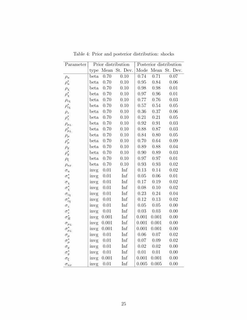
Table 4: Prior and posterior distribution: shocks
Parameter Prior distribution Posterior distributiontype Mean St. Dev. Mode Mean St. Dev.
ρu beta 0.70 0.10 0.74 0.71 0.07ρ∗u beta 0.70 0.10 0.95 0.84 0.06ρχ beta 0.70 0.10 0.98 0.98 0.01ρ∗χ beta 0.70 0.10 0.97 0.96 0.01ρiχ beta 0.70 0.10 0.77 0.76 0.03ρ∗iχ beta 0.70 0.10 0.57 0.54 0.05ρz beta 0.70 0.10 0.36 0.37 0.06ρ∗z beta 0.70 0.10 0.21 0.21 0.05ρµL beta 0.70 0.10 0.92 0.91 0.03ρ∗µL beta 0.70 0.10 0.88 0.87 0.03ρµ beta 0.70 0.10 0.84 0.80 0.05ρ∗µ beta 0.70 0.10 0.70 0.64 0.09ρg beta 0.70 0.10 0.89 0.88 0.04ρ∗g beta 0.70 0.10 0.90 0.89 0.03ρξ beta 0.70 0.10 0.97 0.97 0.01ρnx beta 0.70 0.10 0.93 0.93 0.02σu invg 0.01 Inf 0.13 0.14 0.02σ∗u invg 0.01 Inf 0.05 0.06 0.01σχ invg 0.01 Inf 0.17 0.19 0.02σ∗χ invg 0.01 Inf 0.08 0.10 0.02σiχ invg 0.01 Inf 0.23 0.24 0.04σ∗iχ invg 0.01 Inf 0.12 0.13 0.02σz invg 0.01 Inf 0.05 0.05 0.00σ∗z invg 0.01 Inf 0.03 0.03 0.00σ∗R invg 0.001 Inf 0.001 0.001 0.00σµL invg 0.001 Inf 0.001 0.001 0.00σ∗µL invg 0.001 Inf 0.001 0.001 0.00σµ invg 0.01 Inf 0.06 0.07 0.02σ∗µ invg 0.01 Inf 0.07 0.09 0.02σg invg 0.01 Inf 0.02 0.02 0.00σ∗g invg 0.01 Inf 0.01 0.01 0.00σξ invg 0.001 Inf 0.001 0.001 0.00σnx invg 0.01 Inf 0.005 0.005 0.00
25

Table 6: Variance decomposition - periphery
Variable \ Shock Housingdemand
Housingsupply
Otherdemand
Othersupply
Monetary Foreign
GDP-I 41.2 17.3 7.2 13.3 4.4 16.7Consumption 47.6 22.5 9.1 12.8 2.2 5.9Residential investment 31.2 65.1 0.6 2.2 0.1 0.9Mortgage loans 43.9 17.4 2.3 30.3 0.3 5.9Real house prices 55.1 22.7 4.2 10.8 2.0 5.2Mortgage interest rate 1.1 0.6 18.8 5.3 20.5 53.8Inflation 0.3 0.3 0.3 93.9 0.9 4.4
Note: The shock groupings are as follows. Housing preference, housing investment and monetary policy shocks that hit the
periphery have their own groups called ’Housing demand’, ’Housing supply’ and ’Monetary’, respectively. ’Other demand’
group collects the periphery’s time preference, loan markup and government spending shocks. Technology and product
markup shocks of the periphery populate ’Other supply’ group. ’Foreign’ group aggregates all shocks originating outside of
the periphery, as well as the risk premium and rest of the world net exports shocks.
Table 7: Welfare effects of optimized policies
Agent \ Policy Monetarypolicy
Macroprudentialpolicy
Bothpolicies
Patient (periphery) 0.00 -0.00 -0.00Impatient (periphery) 0.40 1.12 1.20Patient (core) 0.00 -0.00 -0.00Impatient (core) 0.26 0.24 0.26All agents 0.16 0.23 0.24
Note: The table presents the welfare gains on the counterfactual path over the historical path. Gains are expressed in percent
of steady state consumption.
26
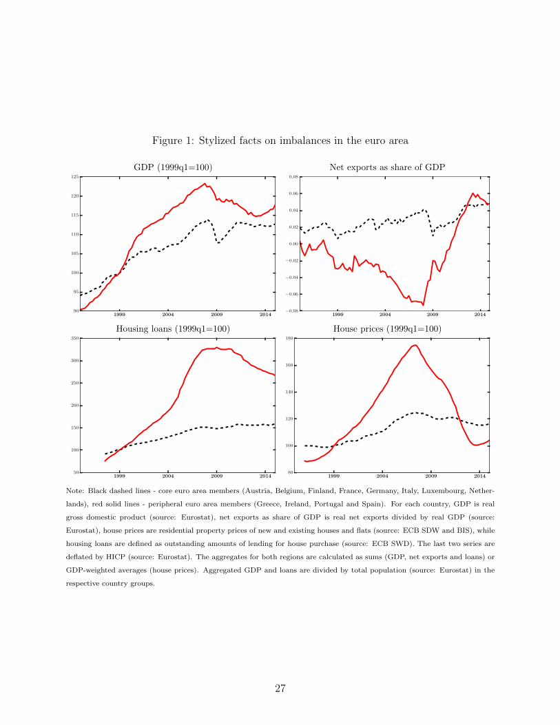
Figure 1: Stylized facts on imbalances in the euro area
GDP (1999q1=100) Net exports as share of GDP
1999 2004 2009 201490
95
100
105
110
115
120
125
1999 2004 2009 2014−0.08
−0.06
−0.04
−0.02
0.00
0.02
0.04
0.06
0.08
Housing loans (1999q1=100) House prices (1999q1=100)
1999 2004 2009 201450
100
150
200
250
300
350
1999 2004 2009 201480
100
120
140
160
180
Note: Black dashed lines - core euro area members (Austria, Belgium, Finland, France, Germany, Italy, Luxembourg, Nether-
lands), red solid lines - peripheral euro area members (Greece, Ireland, Portugal and Spain). For each country, GDP is real
gross domestic product (source: Eurostat), net exports as share of GDP is real net exports divided by real GDP (source:
Eurostat), house prices are residential property prices of new and existing houses and flats (source: ECB SDW and BIS), while
housing loans are defined as outstanding amounts of lending for house purchase (source: ECB SWD). The last two series are
deflated by HICP (source: Eurostat). The aggregates for both regions are calculated as sums (GDP, net exports and loans) or
GDP-weighted averages (house prices). Aggregated GDP and loans are divided by total population (source: Eurostat) in the
respective country groups.
27
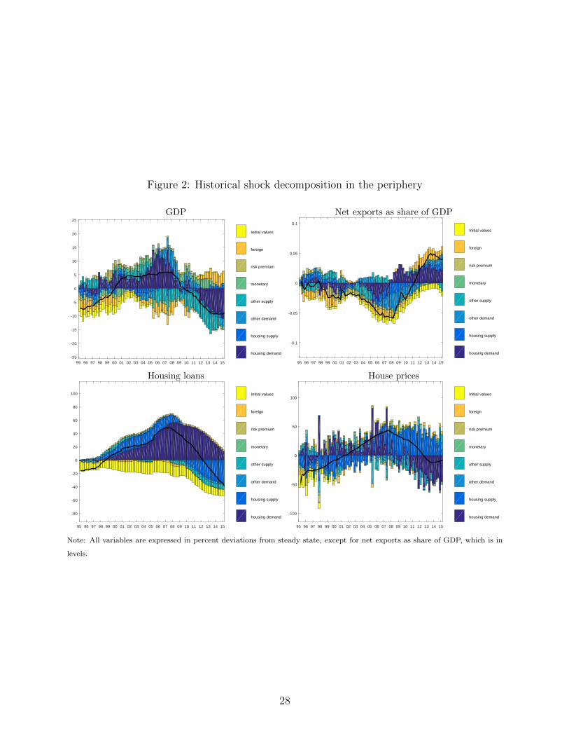
Figure 2: Historical shock decomposition in the periphery
GDP Net exports as share of GDP
95 96 97 98 99 00 01 02 03 04 05 06 07 08 09 10 11 12 13 14 15-25
-20
-15
-10
-5
0
5
10
15
20
25
housing demand
housing supply
other demand
other supply
monetary
risk premium
foreign
Initial values
95 96 97 98 99 00 01 02 03 04 05 06 07 08 09 10 11 12 13 14 15
-0.1
-0.05
0
0.05
0.1
housing demand
housing supply
other demand
other supply
monetary
risk premium
foreign
Initial values
Housing loans House prices
95 96 97 98 99 00 01 02 03 04 05 06 07 08 09 10 11 12 13 14 15
-80
-60
-40
-20
0
20
40
60
80
100
housing demand
housing supply
other demand
other supply
monetary
risk premium
foreign
Initial values
95 96 97 98 99 00 01 02 03 04 05 06 07 08 09 10 11 12 13 14 15
-100
-50
0
50
100
housing demand
housing supply
other demand
other supply
monetary
risk premium
foreign
Initial values
Note: All variables are expressed in percent deviations from steady state, except for net exports as share of GDP, which is in
levels.
28

Figure 3: Impulse responses to common housing preference shock
0 5 10 15 200
0.5
1
1.5GDP
Periphery Core
0 5 10 15 200.5
1
1.5
2
2.5
3
3.5Housing investment
0 5 10 15 200
2
4
6
8
10
12House prices
0 5 10 15 20-0.04
-0.02
0
0.02
0.04
0.06
0.08Inflation
0 5 10 15 20-1
-0.8
-0.6
-0.4
-0.2
0
0.2
0.4
0.6Credit-to-GDP ratio
0 5 10 15 20-0.12
-0.1
-0.08
-0.06
-0.04
-0.02
0
0.02
0.04
0.06Current account balance
Note: All variables are expressed in percent deviations from steady state.The credit-to-GDP ratio and inflation are annualized.
Figure 4: Impulse responses to macroprudential policy shocks in the periphery
0 5 10 15 20 25 30 35 40-0.2
0
0.2
0.4
0.6
0.8GDP
0 5 10 15 20 25 30 35 40-0.5
0
0.5
1
1.5Consumption
0 5 10 15 20 25 30 35 40-0.4
-0.3
-0.2
-0.1
0
0.1
0.2Residential investment
0 5 10 15 20 25 30 35 40-0.015
-0.01
-0.005
0
0.005
0.01
0.015Interest rate
0 5 10 15 20 25 30 35 40-8
-6
-4
-2
0
2×10⁻³ Inflation
0 5 10 15 20 25 30 35 400
0.01
0.02
0.03
0.04Real exchange rate
0 5 10 15 20 25 30 35 400
0.2
0.4
0.6
0.8
1
1.2LTV constraint
0 5 10 15 20 25 30 35 400
0.1
0.2
0.3
0.4
0.5Housing loans
0 5 10 15 20 25 30 35 40-2
0
2
4
6Real house price
LTV shock
Note: All variables are expressed in percent deviations from steady state. Macroprudential rule follows a pure AR(1) process
with autoregression of 0.9.
29

Figure 5: Impulse responses to monetary policy shocks
0 5 10 15 20 25 30 35 40-2.5
-2
-1.5
-1
-0.5
0
0.5GDP
0 5 10 15 20 25 30 35 40-2.5
-2
-1.5
-1
-0.5
0
0.5Consumption
0 5 10 15 20 25 30 35 40-1
-0.5
0
0.5Residential investment
0 5 10 15 20 25 30 35 40-0.2
0
0.2
0.4
0.6
0.8
1Interest rate
0 5 10 15 20 25 30 35 40-0.15
-0.1
-0.05
0
0.05Inflation
0 5 10 15 20 25 30 35 40-0.02
-0.01
0
0.01
0.02
0.03Real exchange rate
0 5 10 15 20 25 30 35 40-1
0
1
2
3LTV constraint
0 5 10 15 20 25 30 35 40-0.4
-0.2
0
0.2
0.4Housing loans
0 5 10 15 20 25 30 35 40-15
-10
-5
0
5Real house price
constant LTV active macroprudential
Note: All variables are expressed in percent deviations from steady state. Macroprudential policy parameters in the active
scenario are: γml = −0.06, γmp = −0.90, γ∗ml = −0.06, γ∗mp = −0.80.
Figure 6: Historical and counterfactual paths under optimal monetary policy maximizingwelfare
98 00 02 04 06 08 10 12 14 161
1.1
1.2
1.3GDP in periphery
98 00 02 04 06 08 10 12 14 161
1.05
1.1
1.15GDP in core
98 00 02 04 06 08 10 12 14 161
2
3
4Credit in periphery
98 00 02 04 06 08 10 12 14 161
1.2
1.4
1.6
1.8Credit in core
98 00 02 04 06 08 10 12 14 160.99
1
1.01
1.02Inflation in periphery
98 00 02 04 06 08 10 12 14 160.995
1
1.005
1.01
1.015Inflation in core
98 00 02 04 06 08 10 12 14 16-0.1
-0.05
0
0.05Net exports in periphery
98 00 02 04 06 08 10 12 14 160.995
1
1.005
1.01
1.015Interest rate
counterfactual historical
Note: All variables are expressed in levels. Monetary policy parameters in the counterfactual scenario are: γ∗π = 1, γ∗y = 0.36.
30

Figure 7: Historical and counterfactual paths under optimal macroprudential policy maxi-mizing welfare
98 00 02 04 06 08 10 12 14 161
1.1
1.2
1.3GDP in periphery
98 00 02 04 06 08 10 12 14 161
1.05
1.1
1.15GDP in core
98 00 02 04 06 08 10 12 14 161
2
3
4Credit in periphery
98 00 02 04 06 08 10 12 14 161
1.2
1.4
1.6
1.8Credit in core
98 00 02 04 06 08 10 12 14 160.4
0.6
0.8
1LTV in periphery
98 00 02 04 06 08 10 12 14 160.65
0.7
0.75
0.8
0.85LTV in core
98 00 02 04 06 08 10 12 14 16-0.1
-0.05
0
0.05Net exports in periphery
98 00 02 04 06 08 10 12 14 161
1.005
1.01
1.015Interest rate
counterfactual historical
Note: All variables are expressed in levels. Macroprudential policy parameters in the counterfactual scenario are:
γml = −0.06, γmp = −0.90, γ∗ml = −0.06, γ∗mp = −0.80.
Figure 8: Historical and counterfactual paths under cooperating optimal monetary andmacroprudential policies maximizing welfare
98 00 02 04 06 08 10 12 14 161
1.1
1.2
1.3GDP in periphery
98 00 02 04 06 08 10 12 14 161
1.05
1.1
1.15GDP in core
98 00 02 04 06 08 10 12 14 161
2
3
4Credit in periphery
98 00 02 04 06 08 10 12 14 161
1.2
1.4
1.6
1.8Credit in core
98 00 02 04 06 08 10 12 14 160.4
0.6
0.8
1LTV in periphery
98 00 02 04 06 08 10 12 14 160.65
0.7
0.75
0.8
0.85LTV in core
98 00 02 04 06 08 10 12 14 16-0.1
-0.05
0
0.05Net exports in periphery
98 00 02 04 06 08 10 12 14 161
1.005
1.01
1.015Interest rate
counterfactual historical
Note: All variables are expressed in levels. Monetary policy parameters in the counterfactual scenario are: γ∗π = 1, γ∗y = 0.26.
Macroprudential policy parameters in the counterfactual scenario are: γml = −0.05, γmp = −0.85, γ∗ml = 0.00, γ∗mp = −0.7.
31