Embed Size (px)
Citation preview

July, 2006
Cost Pass-Through in Differentiated Product Markets: The Case of U.S. Processed Cheese
Donghun Kim∗
Ronald W. Cotterill
International University of Japan and University of Connecticut, respectively. Corresponding coauthor,
Donghun Kim, [email protected], International Development Program, International University of Japan,
Kokusai-cho, Minami Uonuma-shi, Niigata 949-7277, Japan. Fax:81-25-779-1187, Tel:81-25-779-1413.
We would like to thank Robert T. Masson, Oleg Melnikov, Ted O’Donoghue, and George Jakubson for
valuable suggestions. We are also grateful to anonymous referees and Editor Ken Hendricks for helpful
comments.

Cost Pass-Through in Differentiated Product Markets: The Case of U.S. Processed Cheese
ABSTRACT
In this paper, we estimate a mixed logit model for demand in the U.S. processed
cheese market. The estimates are used to determine pass-through rates of cost changes
under different behavioral regimes. We find that, under collusion, the pass-through
rates for all brands fall between 21% and 31% while, under Bertrand-Nash price
competition, the range of pass-through rates are between 73% and 103%. The mixed
logit model provides a more flexible framework for studying pass-through rates than
the logit model since the curvature of the demand functions depends upon the
empirical distribution of consumer types.
JEL: D40, D60, L13, L66, H20
Keyword: Market Structure, Cost Pass-Through, Consumer Welfare, Mixed Logit

1
I. Introduction
In this paper we estimate cost pass-through rates in the market for processed cheese
under Bertrand-Nash pricing and collusive pricing. Cost pass-through rates measure
the proportion of a change in input costs that is passed through to price. A cost change
may arise from various sources, including input price changes or changes in state or
federal taxes. In processed cheese, the main input is raw milk. A frequently asked
question in this market is: what is the impact of an increase in raw milk prices on
cheese prices, consumer surplus, and profits? Our estimates of the cost-pass through
rate provide an answer to these questions.
Early studies of cost pass-through have focused on two polar cases, perfect
competition and monopoly. Under perfect competition, pass-through is determined by
the relative demand and supply elasticities. The pass-through rate is greater when
demand is more inelastic and supply more elastic; it is 100% when input supply is
infinitely elastic. By contrast, the monopolist passes through only 50% of an input cost
change when input supply is infinitely elastic and demand is linear (Bulow et al. 1983).
Several studies have analyzed the effects of cost shocks under imperfect competition
(Stern 1987, Katz & Rosen 1985, and Delipalla & Keen 1992). Most of the theoretical
work have focused on homogeneous products with quantity competition. The
empirical work consists mainly of reduced-form analysis using industry-level data (see,
e.g., Sumner 1981; Sullivan 1985; Karp & Perloff 1989; and Besely & Rosen 1996).
Few studies have studied the effect of cost changes on prices in differentiated product
markets. The exceptions include theoretical studies by Anderson et al. 2001 and Froeb
et al. 2005. The former analyzes the incidence of ad valorem and excise taxes in an
oligopolistic industry with differentiated products and price-setting firms; the latter
investigates the relationship under Bertrand oligopoly between the price effects of

2
mergers absent synergies and the rates at which merger synergies are passed through
to consumers in the form of lower prices.
The main goal of this paper is to estimate cost pass-through rates for a
differentiated product market using a structural model. We first estimate the demand
system for the U.S processed cheese market using a mixed logit model.1 We use the
estimated demands in the firms’ pricing equations to back out estimates of their
marginal costs. We then change marginal costs and solve the model to obtain the new
equilibrium prices.
We use the mixed logit model to estimate demand. This model provides greater
flexibility in substitution patterns than the logit model. In the logit model, the
curvature of demand system, i.e., the second derivatives, is determined by functional
form assumptions; in the mixed logit model, it depends to a significant extent on the
empirical distribution of consumers. This property is important for obtaining accurate
estimates of cost pass-through rates.
We estimate cost pass-through under Bertrand-Nash pricing and fully collusive
pricing in order to evaluate how pass-through depends upon behavior. We find that
cost pass-through rates for the different brands under collusion lie between 21% and
31%. The corresponding pass-through rates under Bertrand-Nash pricing are much
higher, between 73% and 103%. We also estimated the pass-through rates generated
by the logit model to determine the importance of a more flexible specification. We
find that logit pass-through rates are on average 12% lower than those of the mixed
logit model.
1 Refer to BLP 1995 and Nevo 2001. Nevo 2000 applied the model for merger analysis and Petrin 2001 used the model to estimate the consumer benefits of new products in the automobile industry.

3
We compared our pass-through estimates with those obtained from reduced-
form models. Roughly speaking, the pass-through elasticities of the reduced-form
model fall between those of Bertrand-Nash and collusive pricing. The reduced-form
model does not impose a specific price-setting mechanism. Consequently, if the
reduced form estimates are to be believed, then markups for processed cheese are
lower than the monopoly markups but higher than Bertrand-Nash markups. Reduced
form results are often used to infer competitiveness, but notice that it would be
difficult to draw such inferences without knowing the estimates produced by the
benchmark cases of Bertrand-Nash and full collusion. This is another reason for
adopting a structural approach.
We proceed as follows. In Section II, we discuss the U.S. processed cheese
market and the data. The empirical model is presented in Section III. In Section IV, we
describe the estimation strategy. The empirical results are presented in Section V. In
Section VI, we compare the structural approach to estimating cost-pass through rates
to the reduced form approach. Section VII concludes.
II. Market and Data
Processed cheese is used mostly in sandwiches and cheeseburgers and is typically sold
pre-sliced. According to Mueller et al (1996), the four-firm concentration ratio at the
5-digit SIC level was around 70% during the sample period of 1988-1992. Franklin
and Cotterill (1994) report some additional statistics on the processed cheese market
for 1992. Table 1 shows the volume shares and average prices per pound of the
leading processed cheese brands. Philip Morris, whose brands include Kraft and
Velveeta, is the dominant firm with a volume share of around 50% in 1992. Borden

4
Inc., whose main brands are Borden and Lite Line, is a distant second to Philip Morris
with a combined share of around 8%. The other national manufacturers, Land O’Lakes
and H. J. Heinz Co., have very small volume shares. The value of shipments was
US$5.6 billion.
The data for this study was obtained from Information Resources Inc., which
collects quantity and price data from supermarkets in the most populous metropolitan
areas in the U.S. The price and quantity data are quarterly, and cover the first quarter
of 1988 to the fourth quarter of 1992. The number of cities ranges from 28 in the first
quarter of 1988 to 43 in the fourth quarter of 1992. Each city and quarter combination
is defined as a market so there are 680 markets represented in the data. We focused on
ten major brands. The number of brands varies from 7 to 10, depending on markets,
because of the unbalanced nature of the dataset.
The product characteristics of each brand consist of calories, fat, cholesterol
and sodium. Their values were obtained from nutrient fact books that were published
during the sample period.
Demographic information for each city in our sample was obtained from the
Current Population Survey (CPS). The information includes income, age, number of
children, and race. The selection of demographic variables is based on previous
studies of the cheese industry, which includes Gould et al. 1994, Hein et al.1990, and
Gould 1992.
Table 2 gives the market shares, prices and values of the product
characteristics for the ten brands. The market share for each brand is calculated under
the assumption that market size is equal to one serving (28g) per person times the
number of persons in the market. The low numbers reflect the fact that most people do
not buy processed cheese. The price is measures as cents per serving. It is net of any

5
merchandising activity. Thus, a price reduction for a promotion is reflected in the price.
Price is deflated using the regional city CPI and converted to real price per serving.
Table 3 provides summary statistics on the demographic variables. Income is
household income divided by the number of household members. The variable Child
is a binary variable that is equal to 1 if age is less than 17 years old and 0 otherwise.
The binary variable Nonwhite is equal to 1 if an individual is nonwhite and 0
otherwise.
III. Model
In this section we first specify the model of demand, then derive the pricing
equations under different behavioral assumptions, and finally derive the pass-through
equations.
The Demand Equations
Demand for processed cheese is estimated using a discrete choice model
similar to those of BLP 1995 and Nevo 2001.2 Consumers choose one unit of only one
brand in each shopping trip and they choose the brand that offers them the highest
utility. The indirect utility of consumer i from brand j in market m is given by
):,,,,( θξ iijmjmjmijm vDpxU , where jmx are observed cheese characteristics, jmp is
price, iD are observed consumer characteristics, iv and jmξ are unobserved individual
characteristics and unobserved cheese characteristics, respectively. Here θ is an
unknown parameter vector to be estimated. Following Berry 1994, we specify the
indirect utility function as: (1) ijmjmjmiijmijm pxu εξαβ ++−= ,
2 An alternative approach to solving the dimensionality problem in differentiated product markets is to use a multi-level demand system for differentiated products (Hausman, Leonard, & Zona 1994), which is an application of multi-stage budgeting.

6
where iα is consumer i ’s marginal income utility, iβ represents individual specific
parameters, and ijmε is a mean zero stochastic term. Thus, the parameters of the utility
function are different for each consumer. By contrast, in the logit model, the
parameters are the same for all consumers and consumer heterogeneity is modeled in
the error term only.
The indirect utility can be divided into two parts. The first part is the mean utility level of brand j in market m , jmδ , and the second part is the deviation from the
mean level utility, which captures the effects of the random coefficients, ijmµ .
(2) ijmiijmjijmjmjmjjmijm Dvpxpxu εθµθξδ ++= );,,,():,,( 21
(3) jmjmjmjm px ξαβδ +−=
(4) ∑∑∑∑===
++=
+++=K
kjkmikk
K
kjkmillk
L
ljmKiKjmill
L
lijm xvxDpvpD
111)1(1
1σφσηµ
(5) iommiimmi vDu εσφξ +++= 00000
Hence the coefficients on the mean utility function are the same for all individuals and the deviation from the mean utility, ijmµ , depends on the consumer’s observed
characteristics, iD , and unobserved characteristics, iv . The unobserved individual
characteristics are random draws from the multivariate normal distribution, 1,0( +KIN ),
where 1+K draws for each individual correspond to the price and product
characteristics, of which the dimension is 1×K .
Equation (5) represents the utility of an outside good, which is normalized to
0i m iomu ε= . Without an outside good, a simultaneous increase in the prices of inside
goods results in no change in aggregate consumption. The share of outside goods is
defined as the total size of the market minus the shares of inside goods. We follow
Nevo 2001 and assume that the size of the market is one serving of processed cheese
per capita per day. BLP 1995 used the number of households as market size.

7
Let jmA represent the set of values of vD, , and ε that induces the choice of
brand j in market m .
(6) },,,,1,0|,,{ JhuuvDA ihmijmjm =∀>= ε
We assume that vD, , and ε are independently distributed. Here D is drawn from the
empirical distribution, F, obtained from the Current Population Survey; v are drawn
from a multivariate normal distribution, N; and ε is drawn from an extreme value
distribution. Integrating out the idiosyncratic preference shock, the market share of
brand j in market m can be expressed as follows:
(7) 2 ,
( , , ; ) ( ) ( )jm ijmD vs x p s dF D dN vδ θ = ∫
Where 1exp( ) /(1 exp( )Jijm jm ijm sm ismss δ µ δ µ
== + + +∑ , is the probability of individual
i purchasing the product j.
The Pricing Equations
Each firm f , f = 1,.., F, produces goods j = 1,…., fJ . Marginal costs are
constant for each product but vary across markets. Thus, firm f’s profit in market m 3
is given by
(8) ∑ =
−=Π fJ
j jmjmjmmf pMsmcp
1)()(
where jmmc is marginal cost of product j in market m, M is market size, and jms (p) is
the market share of j in market m .
3 In this paper we assume that firms solve a profit maximization problem in each market separately rather than coordinating pricing across markets.

8
Suppose first that firms in the processed cheese market choose their prices
simultaneously and independently. Given the prices of other brands, firm f’s prices
satisfy the first-order conditions
(9) ∑ ===
∂∂
−+=∂
Π∂fJ
k fjm
kmkmkmjm
jm
mf Jj
ps
mcpsp 1
,.......,1,0)(
Note that the second term takes into account the impact of jmp on the revenues of the
firm’s other brands as well as on brand j. In other words, each firm behaves like a
monopolist with respect to its brands.
Suppose next that the firms collude and choose their prices to maximize their
joint profits. The first-order condition for joint profit FΠ maximization is:
(10) ∑ ∑∑= =
≠=
=∂∂
−+∂∂
−+=∂Π∂ f fJ
kJs
jm
smsmsm
F
fffjm
kmkmkmjm
jm
mF
ps
mcpps
mcpsp 1 1
'1'
0)()( '
where ',.......,1 fJs = fJj ,.......,1=
In this case, each firm takes into account the effect of a change in the prices of its
brands on revenues of own and other firms’ brands.
The first-order conditions, (9) and (10), can be summarized in vector notation
as (11): (11) 0)()()( =+∆− pspmcp
where p is the vector of all brand prices, mc is the vector of marginal costs of all
brands, and s (p) is the vector of market shares. Here JJ *=∆ is a matrix with
elements;

9
k
j
s ( ) , if brands k and j are produced by the same firm in the Nash model p
or by a colluder in the collusion model
0 , Otherwise
p∂⎧⎪ ∂⎪⎪⎨⎪⎪⎪⎩
From (11), we can solve for marginal cost for each brand for each market as follows:
(12) ^
1( ) ( )mc p p s p−= + ∆
Thus, the estimated marginal cost depends on the equilibrium price, the parameters of
the demand system, and whether the firms behave non-cooperatively or collude.
The Pass-Through Equations
From (11) we can also estimate the cost pass-through rate analytically. Rewrite
(11) as 0)()()( =+∆−= pspmcpQ . Then, using the implicit function theorem, the
pass-through rate matrix can be derived as follows:
(13) )()( 1
mcQ
pQ
mcp
∂∂
∂∂
−=∂∂ −
The pass-through rate depends on the first and second derivatives of the market share
function. In the mixed logit model, these derivatives depend on the empirical
distribution of observable consumer characteristics and have to be estimated. By
contrast, in the logit model, the derivatives follow directly from functional form
assumptions (Froeb et al. 2005).
Let’s assume that there is a discrete industry-wide common shock for each
brand in each market so marginal cost changes from ^
mc to _
mc . Following the cost
shock, market prices will converge to a new equilibrium. The new equilibrium price
vector is:
(14) 1( ) ( )New New Newp mc p s p−
−= − ∆

10
The price pass-through rate is defined as the ratio of the price change to the change in
marginal cost:
(15) 100×∆∆
=mcpRateThroughPass ,
where p∆ is the difference between the new equilibrium price that solves System (14)
and the old price and ^
mcmcmc −=∆−
. We perturb System (14) with marginal cost
shocks of varying sizes.
As prices change with marginal cost shocks, consumer welfare will change
accordingly. The change in consumer welfare is estimated using the compensating
variation criterion. It measures the amount of income that is needed to keep the
consumer at the same utility level after a price change occurs (e.g., McFadden 1981,
Small & Rosen, 1983, Nevo 2000a). We estimate the consumer welfare changes for
each regime of competition. For price pass-through simulations and consumer welfare
calculations analysis, we assume that neither the marginal utility of consumer income
following cost shocks nor the utility from outside goods changes.
IV. Estimation
To estimate the demand function, we must control for any correlation between prices
and the error term in the mean utility function. The error term represents product
characteristics that are observed by consumers but not by the econometrician. This
correlation is likely to be positive because higher quality could lead suppliers to set
higher prices. For example, Trajtenberg (1989, 1990) found that demand for CT
scanners was estimated to be positively sloped with price because of the omission of
unobserved quality, which was positively correlated with price.
To control for the endogeneity of price, we need to find variables that are
correlated with price but are independent of unobserved product characteristics.

11
Estimation requires an instrument vector with a rank at least equal to the
dimensionality of the parameter vectors. One of the instruments typically used is a
variable that represents closeness in product space in the particular markets (BLP 1995,
Bresnahan, Stern, & Trajsenberg 1997). Such instruments are, however, most
appropriate for dynamically changing markets in which product characteristics evolve
continuously. If a market is mature and product characteristics do not change much,
then this instrumental variable will not change across markets and it will as a
consequence have little identifying power. Another approach is to exploit the panel
structure of the data. Examples of this approach are found in Hausman 1994 and Nevo
2001. The identifying assumption is that, controlling for brand-specific means and
demographics, city-specific demand shocks are independent across cities. Given this
assumption, a demand shock for a particular brand will be independent of prices of the
same brand in other cities. Due to the common marginal cost, prices of a given brand
in different cities within a region will be correlated, and therefore can be used as valid
instrumental variables.4 If, however, there is a national or regional demand shock, this
event will increase the unobserved valuation of all brands in all cities and the
independence assumption will be violated. Also, if advertising campaigns and
promotions are coordinated across cities, these activities will increase demand in the
cities that are included in the activities, so the independence assumption will be
violated for those cities.5 We therefore use an additional set of instrumental variables,
proxies for production costs, to check the sensitivity of the results obtained to different
sets of instrumental variables. We create the production cost proxies by multiplying
4 Refer to Bresnahan’s comment on Hausman 1996. 5 A referee suggested that we include brand-level advertising spending as an independent variable to control for aggregate demand shocks. Nevo 2001 is such an example. Unfortunately, our advertising data was not complete and we could not include such a variable in the model.

12
input prices such as the raw milk price, the diesel price, wages, and electricity by
brand dummies to give cross-brand variations.
Let Z be an N-by-L matrix with row kz and )(θξ be an N-by-1 error tem in
mean utility with row kξ . We introduce brand dummies as well as time dummies in the
model. Hence, a brand-specific component and a time-specific component are
removed from the error term in the mean utility. The assumption that the instrumental
variables are orthogonal to the structural error implies 0] )([ =θξkkzE . The
corresponding sample moment is )('1)(1)(1
θξθξθ Zn
zn
mn
kkk == ∑
=
−. Now we search
forθ , which minimizes the GMM objective function. The GMM estimate is
(17) ]'[minargθ^ −−
== mWmqθ
,
where W is a consistent estimate of the inverse of the asymptotic variance
of ).(θ−mn
V. Results
Table 4 reports parameter estimates for the logit model with and without
instrumental variables. Using prices in other cities as the instrumental variable, price
sensitivity increases from 2.786 to 5.397. Under an alternative specification using cost
data as instrumental variables, the price sensitivity was 4.221. The results suggest that
disregarding the correlation between price and unobserved demand shock can cause
downward bias in price sensitivity.
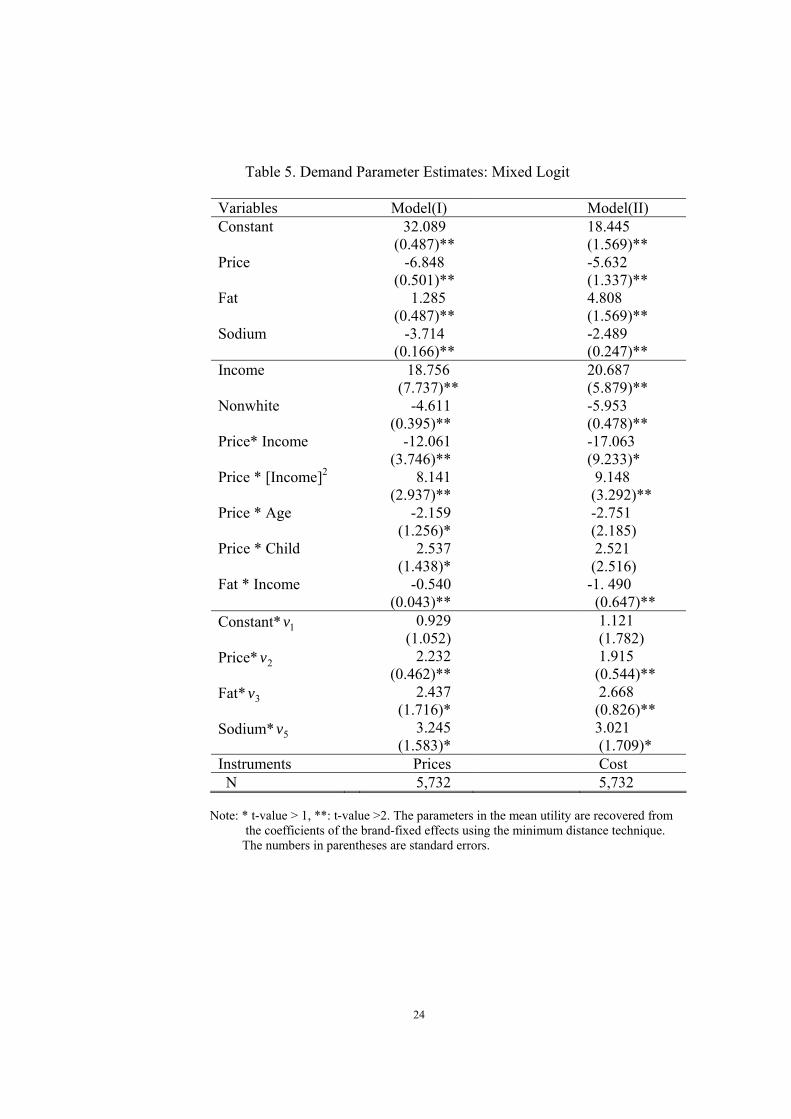
Table 5 reports parameter estimates for the mixed logit model. Here we use
regional prices in other cities and cost variables as instrumental variables for Model I
and Model II, respectively. Overall, the two models yield similar results even though

13
the size of the respective parameter estimates is a bit different. The parameters for the
product characteristics are recovered from those of brand-related fixed effects using
the minimum distance method. The coefficient on PRICE is negative and significant.
The coefficient on FAT is positive and significant, which suggests that the average
consumer prefers the richer taste of higher butterfat despite the higher health risks.
Sensitivity to fat increases, however, as income rises. This phenomenon is captured in
the negative and significant interaction term between fat and income, FAT*INCOME.
SODIUM has a negative and significant effect on the mean utility.
Table 6 reports own- and cross-price elasticities based on the estimates of the
mixed logit model. Each cell (i,j) gives the percent change in market share of brand i
corresponding to a 1 percent change in the price of brand j. Own-price elasticities are
negative but the cross-price elasticities are positive.
Table 7 reports cost estimates under Bertrand-Nash and collusive pricing
respectively. For any vector of prices, marginal costs are lower and markups are
higher markups under collusive pricing than competitive pricing. Recall that equation
(12) implies that the estimated marginal costs are higher for products with higher
market prices and higher values for 1( ) ( )p s p−∆ . For some brands with small market
shares, the elements of the latter term are small negative numbers. Therefore, the
estimated marginal costs are determined mostly by market prices. Accordingly, some
low-fat segment brands, such as Kraft Free, Weight Watchers, and Lite Line, have
high marginal costs. This is particularly true for Lite Line, which has the highest
market price and a very low market share.
Table 8 shows the results of the estimated price pass-through rates. The pass-
through rates are defined as percentage changes in price from a one cent per serving
increase in marginal cost. Under collusion, the pass-through rates for all brands fall in
a narrow range, between 21% and 31%. Under Bertrand-Nash competition, the level

14
of brand pass-through rates increase as does the variation across brands, with rates
ranging between 73% and 103%. To examine the robustness of results, we simulated
the cost pass-through for cost shocks that vary in size from 0.1 cent per serving to 1.2
cents per serving. The results were similar to those reported in Table 8.
Not surprisingly, the simulation results indicate that average pass-through rates
are lower than the rates predicted by a linear demand with a homogenous product.
With constant marginal cost, cost pass-through is 100% in the competitive case and
50% in the monopoly case (Bulow et al. 1983). Note that, in a differentiated product
market, the mixed logit specification allows for price pass-through rates above and
below 100%. Differences in the shape of a brand’s market share function across
markets means that the same brand can have different cost pass-through rates in
different markets.
The curvature of the demand function in the mixed logit model, i.e., the second
derivative of the demand function, is determined by the product characteristics and the
distribution of consumer characteristics. To check on the importance of this flexibility,
we compared the results of the mixed logit model with those of the logit model. Under
Bertrand-Nash pricing, we find that the average pass-through rate in the logit model
for a one-cent per serving change in costs is 71%. This is 12 percent lower than the
average pass-through rate for mixed logit models.
Table 9 shows the change in consumer welfare as measured by the
compensating variation. CV1 and CV2 represent the compensating variations under
Bertrand-Nash and collusive pricing, respectively. In the former case, the CV is 0.63
cents per person for a 1 cent marginal cost decrease and in the latter case, it is 0.23
cents. The ratio of CV2 to CV1 is 37%. Thus, the increase in consumer welfare
following a one cent decrease in cost is substantially lower in the collusive regime
than in the Bertrand-Nash equilibrium.

15
VI. Structural versus Reduced-form Estimates
Reduced-form models have been used extensively in the cost pass-through
literature partly because the analysis is easily implemented. To compare the results of
the structural model with those of a reduced-form model, we use the following
reduced-form model:
(16) 0 1ln( ) *ln( )it i t itprice input Costγ γ ω= + +
Here )ln( itprice is a log of processed cheese prices for brand i and time t,
)ln( tCostinput is a log of input price at time t, and itω represents an error term.
Following Gron and Swenson (2000), we estimate a log-linear regression to obtain a
unit-free measure of the pass-through rate. In our model, 0iγ is a brand fixed effect
and 1γ represents the pass-through elasticity. The brand fixed effects capture time-
invariant markups.
We use raw milk prices, wages, and diesel prices as proxies for input costs.
The milk price is the raw milk price from USDA federal milk order statistics. Wage
and diesel prices are obtained from Bureau of Labor Statistics indices. Table 12
reports summary statistics on the input prices.
Table 10 reports the estimates of the reduced form model. The estimated pass-
through elasticities for milk and diesel prices and wage are 0.034, 0.237, and 0.375,
respectively. In order to compare these estimates to the pass-through rates obtained
from the structural model, we converted them into pass-through elasticities. The pass-
through elasticity is 0.07 for collusive pricing and 0.5 for Nash-Bertrand pricing.
These are the averages for different size cost shocks. The reduced-form results fall
between those of full collusion and Nash price competition. If the reduced-form results
capture the market structure of the processed cheese market correctly, it suggests that

16
the market is less competitive than Bertrand-Nash price competition but more
competitive than collusive pricing. If, however, we do not know the results of
benchmark cases of pass-through elasticities, i. e., those of Bertrand-Nash pricing and
collusion, it may be difficult to infer behavior from the results of a reduced-form
analysis. Meanwhile, if we assume along with many previous studies (e.g., BLP,1995)
that firms behave as posited by Nash-Bertrand model, the reduced form results yield
biased estimates of cost pass-through.
VII. Conclusion
In this paper we estimate a demand system and pricing relationship for a differentiated
product market and implement pass-through simulations and related welfare analysis.
There is a gap in the literature, as analysts have paid little attention to cost pass-
through in differentiated product markets. This study attempts to fill this gap. In the
mixed logit model that we use for demand specification, the curvature of demand
depends on the empirical distribution of consumer characteristics. This property
provides flexible cost pass-through rates that are not driven solely be the functional
form assumption. This paper is the first attempt to examine this issue.
Empirical results indicate that the pass-through rates for the U.S processed
cheese market are greater under Bertrand-Nash pricing than under collusive pricing.
This implies that changes in consumer welfare following cost shocks are greater under
Bertrand-Nash competition. We also compare the results of the structural model with
those of the reduced-form models. We find that the pass-through elasticities of the
reduced-form models fall between those of Bertrand-Nash competition and collusion.
The results suggest that, without knowing the benchmark pass-through elasticities, it

17
may be difficult to infer the degree of market competitiveness from a reduced-form
analysis. They also suggest that the reduced form results are biased.
We have focused here on the Bertrand-Nash equilibrium and collusion. Similar
studies pertaining to other equilibrium concepts, such as semi-collusion and a firm’s
deviation to or from collusion using a cost shock as a focal point, would be possible. A
related avenue would be to analyze a dynamic model that could account for changes in
firm strategies over time. Still another direction for future research would be to
analyze the pass-through rate from manufacturer to retailers and from retailers to
consumers. In this paper we implicitly assume that manufacturers and retailers are
vertically integrated.

18
REFERENCES Anderson, Simon P., Andre de Palma and Brent Kreider, 2001, “Tax Incidence in
Differentiated Product Oligopoly,” Journal of Public Economics 81, 173-192. Besley J. Timothy and Havey S. Rosen, 1998, “Sales Taxes and Prices: An Empirical Analysis,” NBER Working Paper 6667, July. Besley, Timothy, 1989, “Commodity Taxation and Imperfect Competition: A Note on The Effects of Entry,” Journal of Public Economics 40, 359-367. Berry, S., 1994, “Estimating Discrete-Choice Models of Product Differentiation,” Rand Journal of Economics 25, 242-262. Berry, S., Levinsohn, J., and A. Pakes, 1995, “Automobile Prices in Market Equilibrium,” Econometrica 63, 841-889. Bresnahan, F. Timothy , Scott Stern, Manuel Trajtenberg, 1997, “Market Segmentation and the Sources of Rents from Innovation: Personal Computers in the Late 1980s,” Rand Journal of Economics 28, No.0, s17-s44. Bulow I, Jeremy and Paul Pfleiderer, 1983, “A Note on the Effects of Cost Changes on Prices,” Journal of Political Economy 91, Issue 1, February, 181-185. Delipalla, Sofia and Michael Keen, 1992, “The Comparison Between Ad Valorem and
Specific Taxation Under Imperfect Competition,” Journal of Public Economics 49, 351-367.
Fershtman, C, Neil Gandal and Sarit Markovich, 1999, “Estimating the Effect of Tax Reform in Differentiated Product Oligopolistic Markets,” Journal of Public
Economics 74, 151-170. Franklin, Andew W. and Ronald W.Cotterill, 1994, Pricing and Market Strategies in the National Branded Cheese Industry, Food Marketing Policy Center, University of Connecticut. Froeb, Luke and Steven Tschantz and Gregory J. Werden, 2005, “Pass-Through Rates and the Price Effects of Mergers,” International Journal of Industrial Organization 23, 703-715. Gould B.W., 1992, “At-Home consumption of cheese: A purchase-Infrequency Model,” American Journal of Agricultural Economics 74, May, 453-459. Gould B.W. and Huei Chin Lin, 1994, “The Demand for Cheese in the United States:

19
The Role of Household Consumption,” Agribusiness 10-1, January, 43-59. Gron, Anne and Deborah L. Swenson, 2000, “Cost Pass-Through in the U.S. Automobile Market, Review of Economics and Statistics, May, 82(2): 316-324. Hausman, J., 1996, “Valuation of New Goods Under Perfect and Imperfect Competition,” in T Bresnahan and R.Gordon, eds., The Economics of New Goods: Studies in Income and Wealth Vol. 58, Chicago: National Bureau of Economic Research. Hausman, J., G. Leonard, and J.D.Zona, 1994, “Competitive Analysis with Differentiated Products,” Annales D’Economie et de Statistique 34, 159-80. Hein Dale M., Cathy R. Wessels, 1990, “Demand Systems Estimation with Microdata: a Censored Regression Approach,” Journal of Business & Economic Statistics 8-3, 365-371. Karp, Larry and Jeffrey Perloff, 1989, “Estimating Market Structure and Tax Incidence: Japanese Television Market,” Journal of Industrial Economics 38(3), March, 225-239. Katz, Michael and Harvey Rosen, 1985, “Tax Analysis in An Oligopoly Model,” Public Finance Quarterly 13 (January), 3-19. McFadden, D., 1981, “Econometric Models of Probabilistic Choice,” in C. Manski and D. McFadden, eds., Structural Analysis of Discrete Data, 198-272, Cambridge: MIT Press. Mueller, Willard, Bruce W.Marion, Maubool H.Sial, F.E.Geithman,1996, Cheese Pricing: A Study of the National Cheese Exchange, March, Department of Agricultural Economics, University of Wisconsin-Madison. Nevo, Aviv , 2001, “Measuring Market Power in the Ready-To-Eat Cereal Industry,” Econometrica 69, 307-342. Nevo, Aviv, 2000a, “Mergers with Differentiated Products: The Case of the Ready-To-Eat Cereal Industry,” Rand Journal of Economics 31, No.3, 395-421. Nevo, Aviv, 2000b, “ A Practioner’s Guide to Estimation of Random-Coefficients Logit Models of Demand, Journal of Economics & Management Strategy, Vol 9, Number 4, Winter 2000, 513-548. Petrin, A. 2003, ‘ Quantifying the Benefits of New Products: The Case of the Minivan,’ Journal of Political Economy, 110, 705-729.

20
Small, K.A. and Rosen, H.S, 1981, “Applied Welfare Economics with Discrete Choice Models,” Econometrica, Vol. 49, 105-130. Stern, Nicholas H, 1987, “The Effects of Taxation, Price Control and Government Contracts in Oligopoly,” Journal of Public Economics 32, 133-158. Sullivan, Daniel, 1985, “Testing Hypothesis About Firm Behavior in the Cigarette Industry,” Journal of Political Economy 93,586-598. Sumner, Daniel A., 1981, “Measuring of Monopoly Behavior: An Application to the Cigarette Industry,” Journal of Political Economy 89 (October), 1010-1019.

21
Table 1. Leading Processed Cheese Brands, U.S total, 1992
Manufacturer/Brand Volume Share Average Price/lb
Philip Morris Kraft 25.51 3.24 Velveeta 15.56 2.82 Light N Lively 0.59 4.20 Kraft Free 3.65 3.76 Kraft Light 3.19 2.52 Velveeta Light 1.70 3.38 Borden Inc Borden 7.91 2.80 Lite Line 0.53 4.62 Land O’lakes Land O’Lakes 1.28 2.42 HJ Heinz Co Weight Watchers 0.41 3.20
Source: Franklin and Cotterill (1994)

22
Table 2. Market share, Prices, and Product Characteristics
Market Share Price Calories Fat
(g) Cholesterol
(mg) Sodium
(mg)
Kraft 3.172 14.197 90 7 25 380
Velveeta 2.065 12.230 90 6 25 400
Light N Lively 0.098 17.334 70 4 15 406
Kraft Free 0.320 16.541 42 0.3 5 273
Kraft Light 0.173 15.348 70 4 20 160
Velveeta Light 0.233 12.186 60 3 15 430
Borden 0.774 12.931 80 6 20 360
Lite Line 0.0071 19.456 50 2 15 171
Land O’lakes 0.0069 11.990 110 9 26 430
Weight Watchers 0.065 15.376 50 2 7.5 400 Note: Market share (%) and price are the medians for all city-quarter markets. The unit of price is cents per serving (28g).
Table 3. Demographic Variables
Median Mean Std Min Max
Log (Income) 7.923 7.935 0.912 0.396 10.876
Log (Age) 3.478 3.312 0.951 0 4.512
Child 0 0.268 0.436 0 1
Nonwhite 0 0.168 0.362 0 1

23
Table 4. Demand Parameter Estimates: Logit OLS and Logit with IVs
Logit OLS Logit with IVs
Price -2.786
(0.197)
-5.397
(0.445)
-4.221
(0.397)
Time Dummies O O O
Brand Dummies O O O
Instruments X Prices Cost
R2 0.676
First Stage R2 0.914 0.855
N 5734 5734 5734
Note: Dependent Variable is )0ln()ln( msjms − . Standard errors are in parentheses.
24
Table 5. Demand Parameter Estimates: Mixed Logit
Variables Model(I) Model(II) Constant 32.089
(0.487)** 18.445
(1.569)** Price -6.848
(0.501)** -5.632
(1.337)** Fat 1.285
(0.487)** 4.808
(1.569)** Sodium -3.714
(0.166)** -2.489
(0.247)** Income 18.756
(7.737)** 20.687
(5.879)** Nonwhite -4.611
(0.395)** -5.953
(0.478)** Price* Income -12.061
(3.746)** -17.063
(9.233)* Price * [Income]2 8.141
(2.937)** 9.148
(3.292)** Price * Age -2.159
(1.256)* -2.751
(2.185) Price * Child 2.537
(1.438)* 2.521
(2.516) Fat * Income -0.540
(0.043)** -1. 490
(0.647)** Constant* 1v 0.929
(1.052) 1.121
(1.782) Price* 2v 2.232
(0.462)** 1.915
(0.544)** Fat* 3v 2.437
(1.716)* 2.668
(0.826)** Sodium* 5v 3.245
(1.583)* 3.021
(1.709)* Instruments Prices Cost N 5,732 5,732
Note: * t-value > 1, **: t-value >2. The parameters in the mean utility are recovered from the coefficients of the brand-fixed effects using the minimum distance technique. The numbers in parentheses are standard errors.

25
Table 6. Own- and Cross-Elasticities
Borden Light Line Weight Watchers
Land O’Lakes Kraft Line N
lively Velveeta Kraft Free Kraft Light Velveeta
Light
Borden -6.56 0.03 0.10 0.22 1.21 0.05 0.87 0.23 0.22 0.36
Light Line 0.12 -4.62 0.02 0.03 0.15 0.04 0.27 0.08 0.04 0.06
Weight Watchers 0.78 0.05 -6.59 0.09 0.25 0.07 0.45 0.49 0.28 0.48
Land O’Lakes 1.09 0.02 0.12 -7.35 0.98 0.08 0.95 0.19 0.60 0.43
Kraft 0.75 0.01 0.04 0.24 -5.07 0.04 1.23 0.16 0.21 0.27
Lite N Lively 0.21 0.06 0.05 0.04 0.67 -3.67 0.54 0.12 0.08 0.10
Velveeta 0.92 0.02 0.07 0.21 1.18 0.05 -6.29 0.21 0.20 0.46
Kraft Free 0.39 0.02 0.12 0.03 0.11 0.04 0.62 -4.39 0.36 0.41
Kraft Light 0.72 0.03 0.08 0.20 0.61 0.03 0.56 0.35 -5.88 0.25
Velveeta Light 0.96 0.04 0.16 0.13 0.83 0.05 0.83 0.43 0.26 -7.21
Outside Good 0.63 0.02 0.09 0.14 0..23 0.02 0.34 0.14 0.15 0.17
Note: Elasticities are median values for 210 sample markets from the fourth quarter of 1991 to the fourth quarter of 1992. Row is i and column is j. Each cell (i,j) gives the percent change in market share of brand i corresponding to a 1 percent change in the price of brand j.

26
Table 7. Marginal cost, Markup, and Margin
Nash-Bertrand
Full Collusion
Brand MC P-MC (P-MC)/ P*100 MC P-MC (P-MC)/
P*100 Kraft 7.84 6.08 42.65 4.75 9.62 67.75 Velveeta 6.69 5.53 45.03 4.13 8.44 67.97 Light N Lively 10.35 6.12 36.83 7.24 9.97 58.13 Kraft Free 10.59 5.45 34.91 7.75 8.14 51.78 Kraft Light 9.36 5.30 36.34 6.19 8.53 59.16 Velveeta Light 7.81 4.69 37.80 4.98 7.39 61.26 Borden 11.27 1.62 12.72 4.26 8.94 67.45 Lite Line 18.13 1.89 10.58 10.37 9.43 49.11 Land O’Lakes 10.56 1.37 11.70 3.62 8.37 70.74 Weight Watchers 12.88 1.95 12.58 5.65 9.43 62.51
Note: Median values for all markets. Marginal costs and markups are cents per serving.

27
Table 8. Pass-Through Rate(%)
Nash Bertrand Collusion Kraft 93.61 30.42 Velveeta 91.56 28.74 Light N Lively 88.72 26.45 Kraft Free 90.12 26.98 Kraft Light 99.93 30.34 Velveeta Light 93.29 30.83 Borden 102.89 30.12 Lite Line 73.33 23.70 Land O'Lakes 88.36 21.25 Weight Watchers 76.86 25.45 Overall 82.67 27.04 MC shock 1.0 1.0
Note: Median values for all markets. Marginal cost shocks are cents
per serving.
Table 9. Compensating Variation
Bertrand-Nash (A) 0.63 Collusion (B) 0.23
B/A(%) 37% MC Shock(Cents) 1.0
Note: Cents/per serving/per person, median values for all markets.

28
Table 10. Results of Reduced-Form Models
Independent variables
Dependent Variable: )ln( price
)ln(Milkprice 0.034 (0.019)
- -
)ln(Diesel - 0.237 (0.010)
-
)ln(Wage - - 0.375 (0.029)
2R 0.672 0.702 0.702
Note: Each regression includes brand-fixed effects. The numbers in parentheses are standard errors.
Table 11. Pass-Through Elasticities: Structural model
Nash-Bertrand Competition Collusion 0.47 0.066
Table 12. Input Prices
Mean Std Dev Min Max Milk(US $/ 100
pounds) 11.69 1.03 10.07 14.50
Wage (PPI) 106.78 5.73 95.70 114.50 Diesel (PPI) 63.16 9.55 44.00 91.93


![Example: Automatic detection of pathological ECG-pattern ...pub.ist.ac.at/~schloegl/lv/biosig/biosig2005_chp5.pdfdiff ECG amplitude [arb. units] differentiated and low-pass filtered](https://img.dokumen.tips/doc/110x75/5e8d88c88d16d4748c02205f/example-automatic-detection-of-pathological-ecg-pattern-pubistacatschloegllvbiosigbiosig2005chp5pdf.jpg)