Cosmological Inflation: History and Present Status

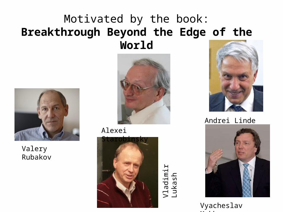
Motivated by the book:Breakthrough Beyond the Edge of the World

Valery Rubakov

Alexei Starobinsky

Andrei Linde

Vyacheslav Mukhanov

Vla

dim

ir Lu

kash

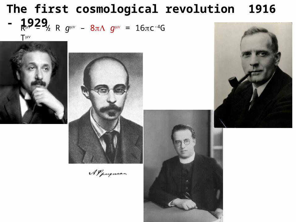
The first cosmological revolution 1916 - 1929

Rmn – ½ R gmn – 8pL gmn = 16pc-4G Tmn

The universe is not just a containment of everything that exists –

This is a physical object!

- Geometry: a closed 3D space + time

- Size: unknown but > 1012 light years

- Dynamics: accelerating expansion

- Density: 10-29 g/сm3

- Equation of state: pressure = 0 (dust)

- Temperature: 2.7о К

- Total energy: 0 (Zero!)

Big Bang problems

- Horizon problem (Charles Misner): Universe is the same in the causally unconnected regions

- Flatness problem (W = 1), or r = rc

- Cosmic junk problem: lack of monopoles, cosmic strings etc.

- Entropy problem: ~ 1090 particles within horizon

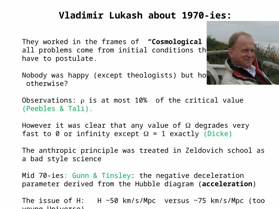
Vladimir Lukash about 1970-ies:

They worked in the frames of “Cosmological postulate”: all problems come from initial conditions that we have to postulate.

Nobody was happy (except theologists) but how to work otherwise?

Observations: r is at most 10% of the critical value (Peebles & Tali).

However it was clear that any value of W degrades very fast to 0 or infinity except W = 1 exactly (Dicke)

The anthropic principle was treated in Zeldovich school as a bad style science

Mid 70-ies: Gunn & Tinsley: the negative deceleration parameter derived from the Hubble diagram (acceleration)

The issue of H: H ~50 km/s/Mpc versus ~75 km/s/Mpc (too young Universe)

Reincarnation of the L-term (cosmological term)

Rmn – ½ R gmn – 8pL gmn = 16pc-4G Tmn

( �̇�𝑎 )2- 8/3pL =

G - e 𝑘𝑅𝑜2𝑎 (𝑡 ) 2

Vacuum (p = - e) 𝑎=𝑒𝑡 𝐻

p = w e 𝑎=𝑡2

3 (1+𝑤)

The first hint:

Brout, Englert & Gunzig 1961 Creation of Universe ex nihilis with a massive scalar field (a toy model)

The next attempt:

Erast Gliner 1969: non-singular bounce due to “heavy vacuum” with p = -e

Contraction -> expansion through de-Sitter stage

Gliner & Dymnikova 1975: It solves problems of flatness (big Universe) and of a large entropy

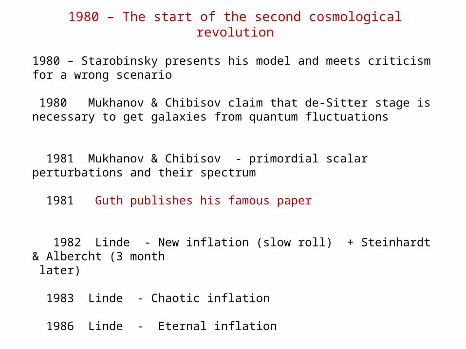
1980 – The start of the second cosmological revolution

1980 – Starobinsky presents his model and meets criticism for a wrong scenario

1980 Mukhanov & Chibisov claim that de-Sitter stage is necessary to get galaxies from quantum fluctuations 1981 Mukhanov & Chibisov - primordial scalar perturbations and their spectrum

1981 Guth publishes his famous paper

1982 Linde - New inflation (slow roll) + Steinhardt & Albercht (3 month later)

1983 Linde - Chaotic inflation

1986 Linde - Eternal inflation

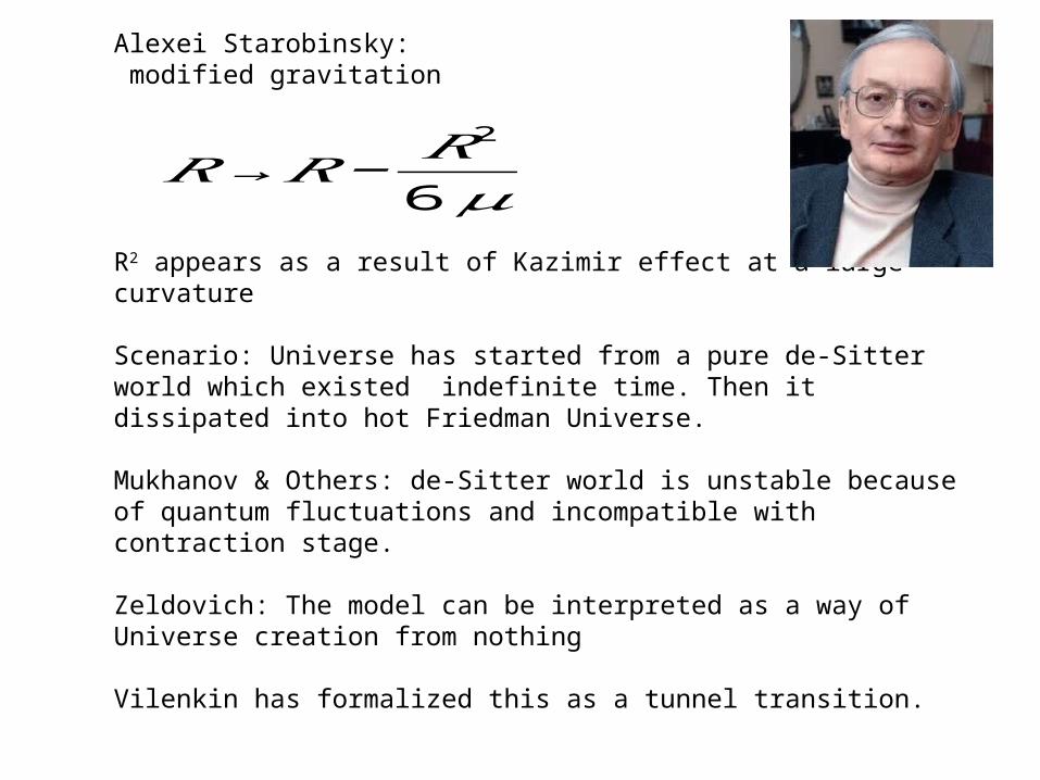
Alexei Starobinsky: modified gravitation

R2 appears as a result of Kazimir effect at a large curvature

Scenario: Universe has started from a pure de-Sitter world which existed indefinite time. Then it dissipated into hot Friedman Universe.

Mukhanov & Others: de-Sitter world is unstable because of quantum fluctuations and incompatible with contraction stage.

Zeldovich: The model can be interpreted as a way of Universe creation from nothing

Vilenkin has formalized this as a tunnel transition.

𝑅→𝑅− 𝑅2

6𝜇

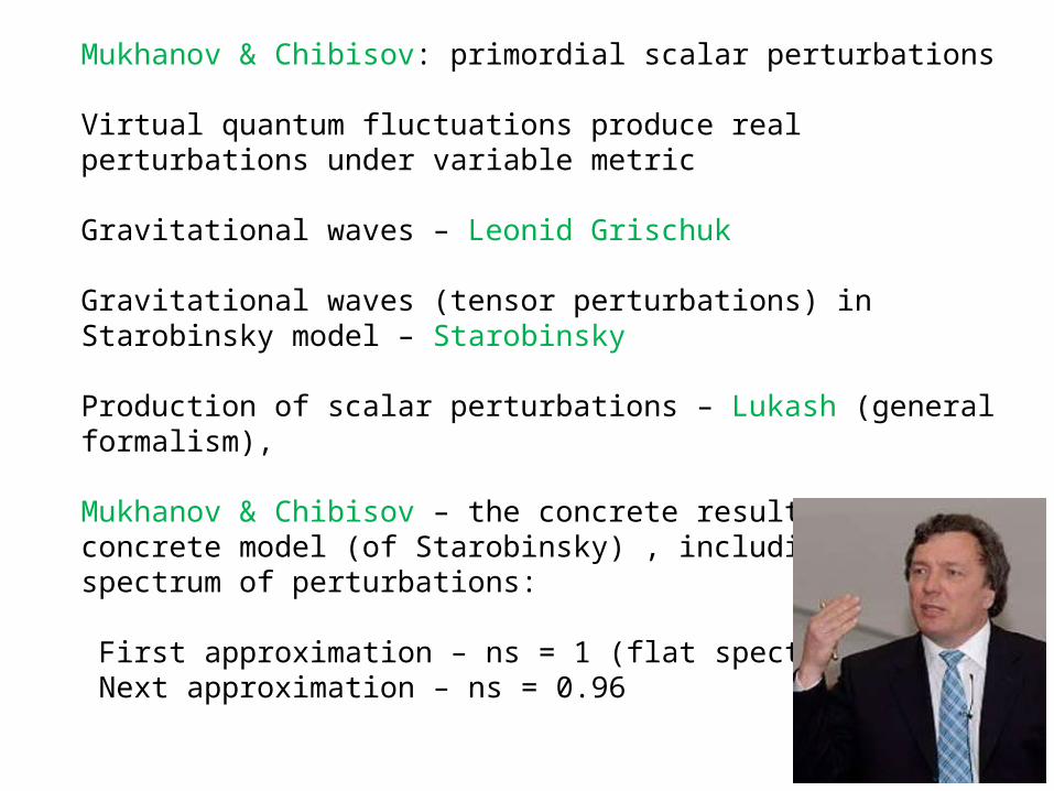
Mukhanov & Chibisov: primordial scalar perturbations

Virtual quantum fluctuations produce real perturbations under variable metric

Gravitational waves – Leonid Grischuk

Gravitational waves (tensor perturbations) in Starobinsky model – Starobinsky

Production of scalar perturbations – Lukash (general formalism),

Mukhanov & Chibisov – the concrete result for the concrete model (of Starobinsky) , including the spectrum of perturbations:

First approximation – ns = 1 (flat spectrum) Next approximation – ns = 0.96

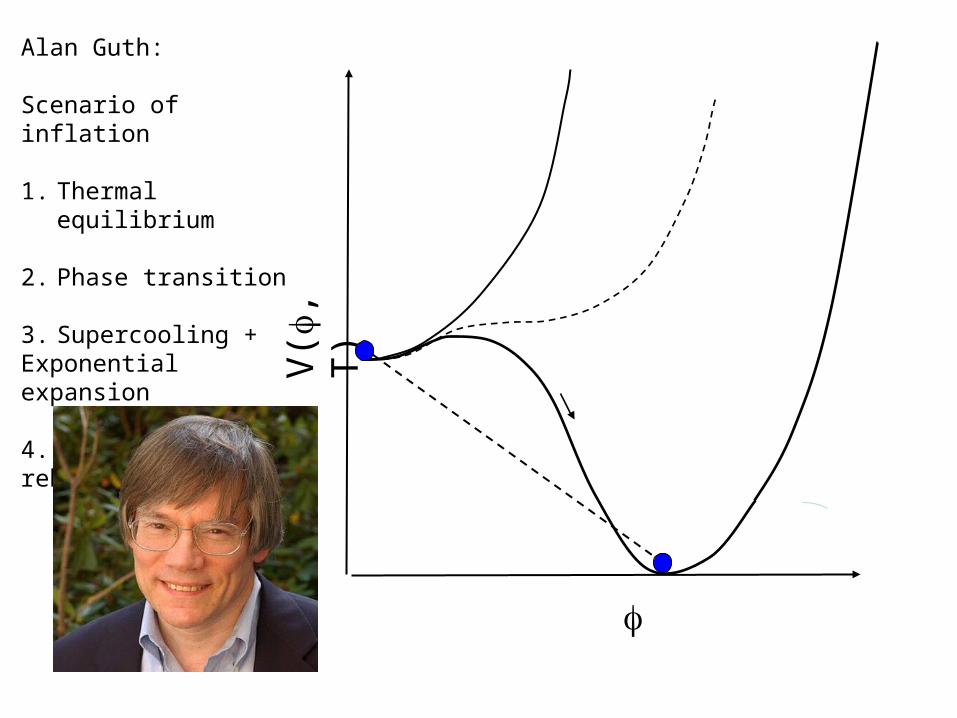
f

V(f

, T)

Alan Guth:

Scenario of inflation

1. Thermal equilibrium

2. Phase transition

3. Supercooling + Exponential expansion

4. “Boiling” – reheating

Answers:

1. The flatness problem is evidently solved with expansion by many orders of magnitude (Wk ~ 10-100, e.g)

2. The horizon problem disappears because all we see inside the horizon was a causally connected piece of a uniform heavy vacuum.

3. All exotic “defects” were swept away during inflation out of the horizon

4. A huge entropy results from the decay of self-reproducing scalar field

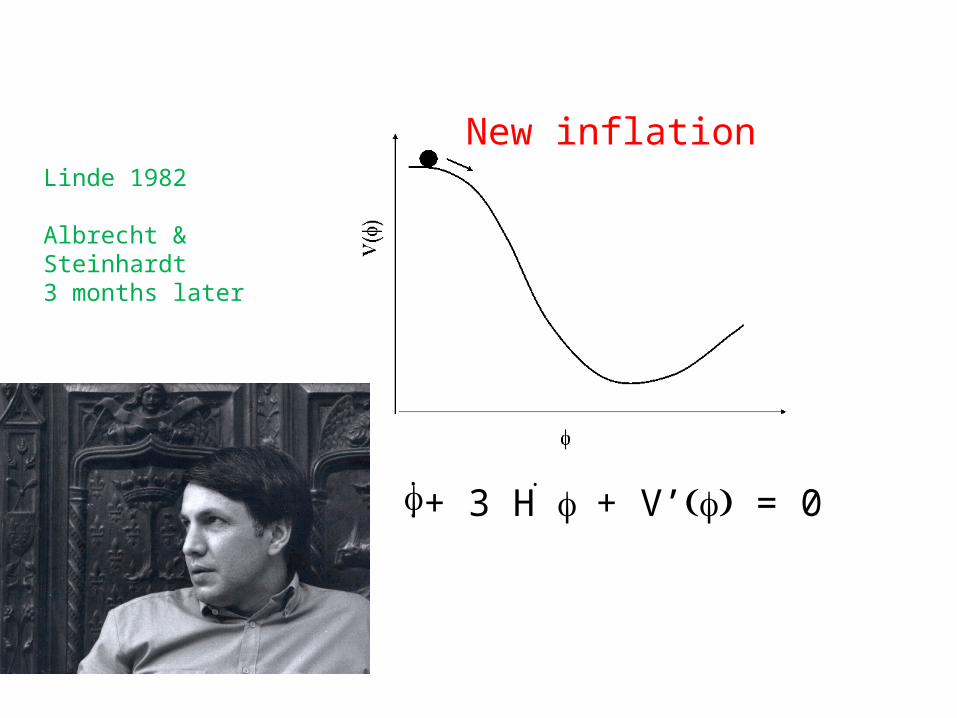
New inflation

f+ 3 H f + V’( )f = 0.. .

Linde 1982

Albrecht & Steinhardt3 months later

Chaotic inflation Linde 1983

f > Mpl

f(x) – homogeneous at ~ 10 Rhor

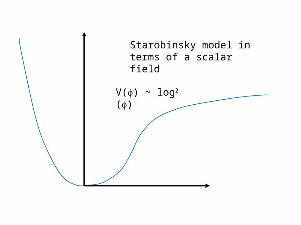
Starobinsky model in terms of a scalar field

V(f) ~ log2 (f)

Ethernal inflation Linde 1986

Planck limit

Andrei Linde

Predictions (According to Slava Mukhanov)

1. Flatness W=1

2. Spectral slope of primordial perturbations ns ~ 0.96 – 0.97

3. Gaussianity

4. Adiabaticity

5. Gravitational waves

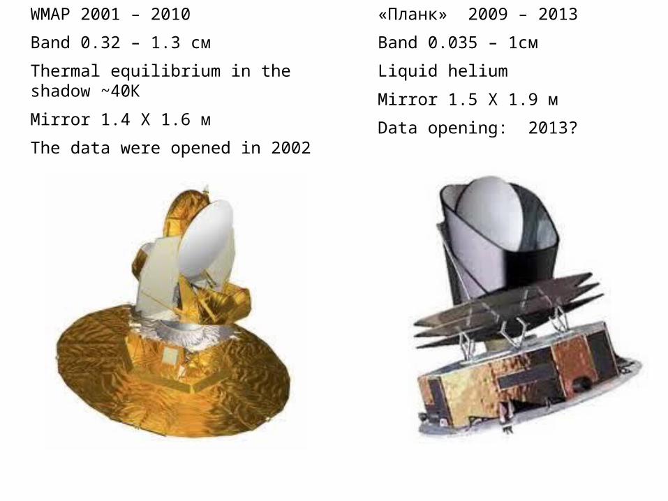
WMAP 2001 – 2010

Band 0.32 – 1.3 см

Thermal equilibrium in the shadow ~40К

Mirror 1.4 Х 1.6 м

The data were opened in 2002

«Планк» 2009 – 2013

Band 0.035 – 1см

Liquid helium

Mirror 1.5 Х 1.9 м

Data opening: 2013?

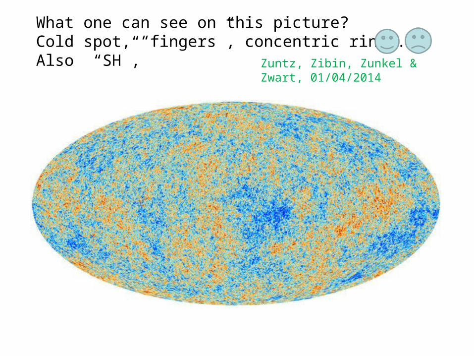
What one can see on this picture?Cold spot, “fingers”, concentric rings. Also “SH”,

Zuntz, Zibin, Zunkel & Zwart, 01/04/2014

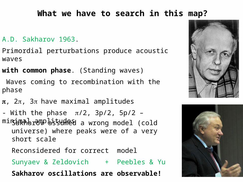
What we have to search in this map?

A.D. Sakharov 1963.

Primordial perturbations produce acoustic waves

with common phase. (Standing waves)

Waves coming to recombination with the phase

p, 2p, 3 p have maximal amplitudes

- With the phase p/2, 3p/2, 5p/2 – minimal amplitudes

Sakharov assumed a wrong model (cold universe) where peaks were of a very short scale

Reconsidered for correct model

Sunyaev & Zeldovich + Peebles & Yu

Sakharov oscillations are observable!

Silk effect

Fit of the multipole spectrum

Free parameters:1. The amplitude of primordial perturbations (normalization)

2. The spectral slope (with a deviation from a flat)

3. The share of the baryonic matter (affects the height of the first peak)

4. The share of the dark matter (affects the ratio between peaks)

5. The curvature parameter W (defines the angular scale of the whole picture)

6. Free electron optical depth (reionization z) affects the curve at low L

-----------------------

Curvature

Wk = 0.001+-0.006

Dark matter

Wc = 0.259+-0.005

Baryonic matter

Wb = 0.048+-0.001

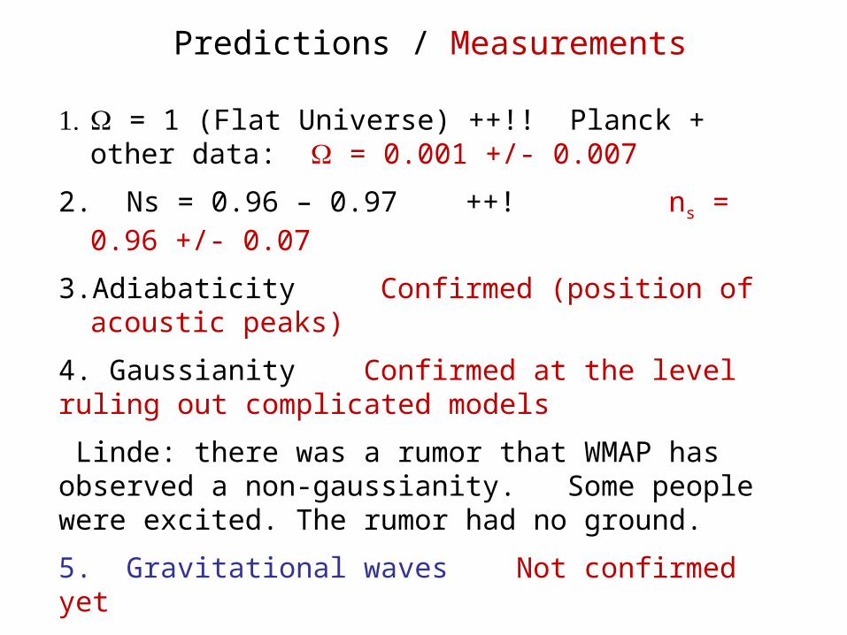
1. W = 1 (Flat Universe) ++!! Planck + other data: W = 0.001 +/- 0.007

2.. Ns = 0.96 – 0.97 ++! ns = 0.96 +/- 0.07

3. Adiabaticity Confirmed (position of acoustic peaks)

4. Gaussianity Confirmed at the level ruling out complicated models

Linde: there was a rumor that WMAP has observed a non-gaussianity. Some people were excited. The rumor had no ground.

5. Gravitational waves Not confirmed yet

Predictions / Measurements

Starobinsky model

BICEP2

It was too early to drink champagne!

BICEP 2

South pole

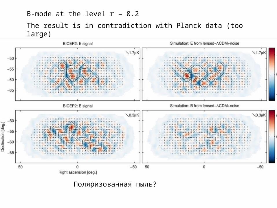
B-mode at the level r = 0.2

The result is in contradiction with Planck data (too large)

Поляризованная пыль?

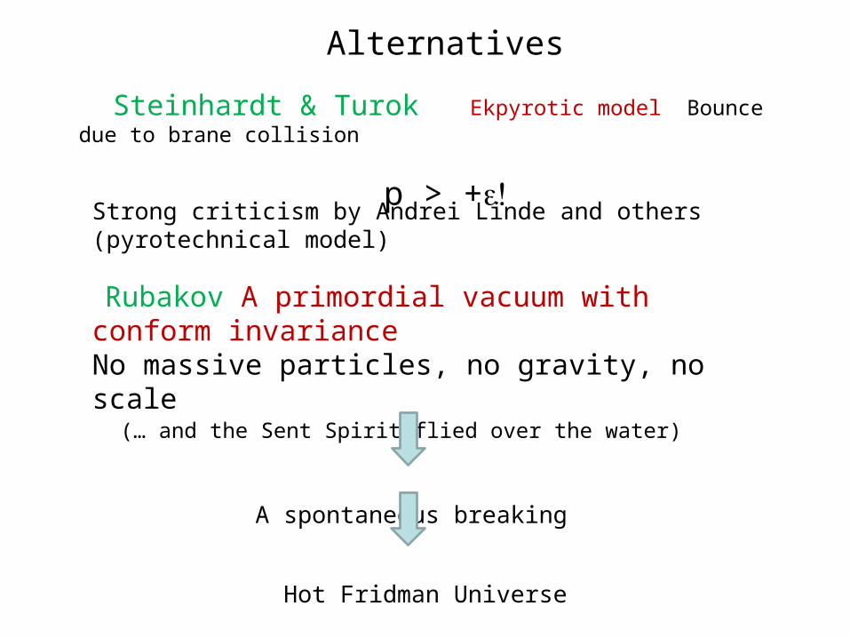
Alternatives

Steinhardt & Turok Ekpyrotic model Bounce due to brane collision

p > + !eStrong criticism by Andrei Linde and others(pyrotechnical model)

Rubakov A primordial vacuum with conform invariance No massive particles, no gravity, no scale (… and the Sent Spirit flied over the water)

A spontaneous breaking

Hot Fridman Universe

Linde, Mukhanov, Stasrobinsky:

Inflation theory is simple (in ideology), solves all problems and has predicted future observations.

Alternatives are more complicated, require additional entities and give no clear predictions

Rubakov:

Until primordial gravitational waves are detected alternative models have a right for existence (and it is worth to wait with Nobel prize)

However, one part of the theory has no alternatives: the quantum production of primordial perturbations by Mukhanov $ Chibisov

My impressions:

- Inflation theory far exceeds alternatives in ideological simplicity and predictive power. Also the most economical in the sense of extra entities.

- Among the inflation models the best is that of Alexei Starobinsky with the same reason.

- William Occam probably would agree with me.