Correlation and Regression Notes - educ.jmu.edueduc.jmu.edu/~drakepp/FIN360/readings/Regression_notes.pdf · 5 Correlation and Regression ... Regression is the analysis of the relation

Contents

Basic terms and concepts ................................................................................................................. 1

Simple regression ............................................................................................................................ 5

Multiple Regression ....................................................................................................................... 13

Regression terminology .................................................................................................................. 20

Regression formulas ...................................................................................................................... 21

Correlation and regression Notes prepared by Pamela Peterson Drake

Notes prepared by Pamela Peterson Drake

1 Correlation and Regression

Basic terms and concepts 1. A scatter plot is a graphical representation of the relation between two or more variables. In

the scatter plot of two variables x and y, each point on the plot is an x-y pair.

2. We use regression and correlation to describe the variation in one or more variables.

A. The variation is the sum of the squared deviations of a variable.

N2

i=1

Variation= x-x

B. The variation is the numerator of the variance of a sample:

N2

i=1

x-x

Variance=N-1

C. Both the variation and the variance are measures of the dispersion of a sample.

3. The covariance between two random variables is a statistical measure of the degree to which the two variables move together.

A. The covariance captures how one variable is different from its mean as the other variable is different from its mean.

B. A positive covariance indicates that the variables tend to move together; a negative covariance indicates that the variables tend to move in opposite directions.

C. The covariance is calculated as the ratio of the covariation to the sample size less one:

N

i i

i=1

(x -x)(y -y)

Covariance = N-1

where N is the sample size xi is the ith observation on variable x, x is the mean of the variable x observations, yi is the ith observation on variable y, and y is the mean of the variable y

observations.

D. The actual value of the covariance is not meaningful because it is affected by the scale of the two variables. That is why we calculate the correlation coefficient – to make something interpretable from the covariance information.

E. The correlation coefficient, r, is a measure of the strength of the relationship between or among variables.

Calculation:

Example1: Home sale prices and square footage

Home sales prices (vertical axis) v. square footage for a sample of 34 home sales in September 2005 in St. Lucie County.

Note: Correlation does not imply causation. We may say that two variables X and Y are correlated, but that does not mean that X causes Y or that Y causes X – they simply are related or associated with one another.

$0

$100,000

$200,000

$300,000

$400,000

$500,000

$600,000

$700,000

$800,000

0 500 1,000 1,500 2,000 2,500 3,000

Salesprice

Square footage



yof

deviation standard

xof

deviation standard

yand x betwen covariancer

N

i i

i=1

N N2 2

i ii=1,n i=1

(x -x) (y -y)

N-1r=

(x -x) (y -y)

N-1 N-1

Example 2: Calculating the correlation coefficient

Deviation

of x

Squared deviation of

x Deviation

of y

Squared deviation of

y Product of deviations

Observation x y x- x (x- x )2 y- y (y- y )2 (x- x )(y- y )

1 12 50 -1.50 2.25 8.40 70.56 -12.60

2 13 54 -0.50 0.25 12.40 153.76 -6.20

3 10 48 -3.50 12.25 6.40 40.96 -22.40

4 9 47 -4.50 20.25 5.40 29.16 -24.30

5 20 70 6.50 42.25 28.40 806.56 184.60

6 7 20 -6.50 42.25 -21.60 466.56 140.40

7 4 15 -9.50 90.25 -26.60 707.56 252.70

8 22 40 8.50 72.25 -1.60 2.56 -13.60

9 15 35 1.50 2.25 -6.60 43.56 -9.90

10 23 37 9.50 90.25 -4.60 21.16 -43.70

Sum 135 416 0.00 374.50 0.00 2,342.40 445.00 Calculations:

x = 135/10 = 13.5

y = 416 / 10 = 41.6

2xs = 374.5 / 9 = 41.611

2ys = 2,342.4 / 9 = 260.267

r = 445/9 49.444

= =0.475(6.451)(16.133)41.611 260.267

i. The type of relationship is represented by the correlation coefficient:

r =+1 perfect positive correlation

+1 >r > 0 positive relationship

r = 0 no relationship

0 > r > 1 negative relationship

r = 1 perfect negative correlation

ii. You can determine the degree of correlation by looking at the scatter graphs.

If the relation is upward there is positive correlation.

If the relation downward there is negative correlation.



0 < r < 1.0 Y

X

-1.0 < r < 0 Y

X

iii. The correlation coefficient is bound by –1 and +1. The closer the coefficient to –1 or +1, the stronger is the correlation.

iv. With the exception of the extremes (that is, r = 1.0 or r = -1), we cannot really talk about the strength of a relationship indicated by the correlation coefficient without a statistical test of significance.

v. The hypotheses of interest regarding the population correlation, , are:

Null hypothesis H0: = 0

In other words, there is no correlation between the two variables

Alternative hypothesis Ha: =/ 0

In other words, there is a correlation between the two variables

vi. The test statistic is t-distributed with N-2 degrees of freedom:1

2r-1

2-Nr t

vii. To make a decision, compare the calculated t-statistic with the critical t-statistic for the appropriate degrees of freedom and level of significance.

1 We lose two degrees of freedom because we use the mean of each of the two variables in performing this test.

Example 2, continued

In the previous example,

r = 0.475

N = 10

2

0.475 8 1.3435t 1.5267

0.881 0.475



Problem Suppose the correlation coefficient is 0.2 and the number of observations is 32. What is the calculated test statistic? Is this significant correlation using a 5% level of significance? Solution Hypotheses: H0: = 0

Ha:

Calculated t-statistic: 0.2 32-2 0.2 30

t = = =1.118031-0.04 0.96

Degrees of freedom = 32-2 = 30

The critical t-value for a 5% level of significance and 30 degrees of freedom is 2.042. Therefore, we conclude

that there is no correlation (1.11803 falls between the two critical values of –2.042 and +2.042).

Problem Suppose the correlation coefficient is 0.80 and the number of observations is 62. What is the calculated test statistic? Is this significant correlation using a 1% level of significance? Solution Hypotheses: H0: = 0

Ha:

Calculated t-statistic: 0.80 62 2 0.80 60 6.19677

t 10.327960.61 0.64 0.36

The critical t-value for a 1% level of significance and 61 observations is 2.665. Therefore, we reject the null

hypothesis and conclude that there is correlation.

F. An outlier is an extreme value of a variable. The outlier may be quite large or small (where large and small are defined relative to the rest of the sample).

i. An outlier may affect the sample statistics, such as a correlation coefficient. It is possible for an outlier to affect the result, for example, such that we conclude that there is a significant relation when in fact there is none or to conclude that there is no relation when in fact there is a relation.

ii. The researcher must exercise judgment (and caution) when deciding whether to include or exclude an observation.

G. Spurious correlation is the appearance of a relationship when in fact there is no relation. Outliers may result in spurious correlation.

i. The correlation coefficient does not indicate a causal relationship. Certain data items may be highly correlated, but not necessarily a result of a causal relationship.

ii. A good example of a spurious correlation is snowfall and stock prices in January. If we regress historical stock prices on snowfall totals in Minnesota, we would get a statistically significant relationship – especially for the month of January. Since there is not an economic reason for this relationship, this would be an example of spurious correlation.



Simple regression 1. Regression is the analysis of the relation between one variable and some other variable(s),

assuming a linear relation. Also referred to as least squares regression and ordinary least squares (OLS).

A. The purpose is to explain the variation in a variable (that is, how a variable differs from it's mean value) using the variation in one or more other variables.

B. Suppose we want to describe, explain, or predict why a variable differs from its mean. Let the ith observation on this variable be represented as Yi, and let n indicate the

number of observations.

The variation in Yi's (what we want to explain) is:

Variationof Y

= N

2

i

i=1

y -y = SSTotal

C. The least squares principle is that the regression line is determined by minimizing the sum of the squares of the vertical distances between the actual Y values and the predicted values of Y.

Y

X

A line is fit through the XY points such that the sum of the squared residuals (that is, the sum of the squared the vertical distance between the observations and the line) is minimized.

2. The variables in a regression relation consist of dependent and independent variables.

A. The dependent variable is the variable whose variation is being explained by the other variable(s). Also referred to as the explained variable, the endogenous variable, or the predicted variable.

B. The independent variable is the variable whose variation is used to explain that of the dependent variable. Also referred to as the explanatory variable, the exogenous variable, or the predicting variable.

C. The parameters in a simple regression equation are the slope (b1) and the intercept (b0):

yi = b0 + b1 xi + i

where yi is the ith observation on the dependent variable,

xi is the ith observation on the independent variable,

b0 is the intercept. b1 is the slope coefficient,

i is the residual for the ith observation.



X

Y

b0

b1

0

D. The slope, b1, is the change in Y for a given one-unit change in X. The slope can be positive, negative, or zero, calculated as:

1N

)x(x

1N

)x)(xy(y

var(X)

Y)cov(X,b

N

1i

2i

N

1i

ii

1

Suppose that:

N

1i

i )x)(xy(y = 1,000

N

1i

2i )x(x = 450

N= 30

Then

1

1,00034.4827629b = = =2.2222

450 15.5172429

E. The intercept, b0, is the line‟s intersection with the Y-axis at X=0. The intercept can be positive, negative, or zero. The intercept is calculated as:

0 1b =y-b x

Hint: Think of the regression line as the average of the relationship between the independent variable(s) and the dependent variable. The residual represents the distance an observed value of the dependent variables (i.e., Y) is away from the average relationship as depicted by the regression line.

A short-cut formula for the slope coefficient:

N NN

i iNi i i 1 i 1i ii 1

i 11 N 22 N

iii 1 N

2 i 1i

i 1

x y(y y)(x x)

x yN

N 1b

(x x)x

N 1 xN

Whether this is truly a short-cut or not depends on the method of performing the calculations: by hand, using Microsoft Excel, or using a calculator.



3. Linear regression assumes the following:

A. A linear relationship exists between dependent and independent variable. Note: if the relation is not linear, it may be possible to transform one or both variables so that there is a linear relation.

B. The independent variable is uncorrelated with the residuals; that is, the independent variable is not random.

C. The expected value of the disturbance term is zero; that is, E( i)=0

D. There is a constant variance of the disturbance term; that is, the disturbance or residual terms are all drawn from a distribution with an identical variance. In other words, the disturbance terms are homoskedastistic. [A violation of this is referred to as heteroskedasticity.]

E. The residuals are independently distributed; that is, the residual or disturbance for one observation is not correlated with that of another observation. [A violation of this is referred to as autocorrelation.]

F. The disturbance term (a.k.a. residual, a.k.a. error term) is normally distributed.

4. The standard error of the estimate, SEE, (also referred to as the standard error of the residual or standard error of the regression, and often indicated as se) is the standard deviation of predicted dependent variable values about the estimated regression line.

5. Standard error of the estimate (SEE) = se2 = ResidualSS

N 2

SEE2N

ε

2N

)y(y

2N

xbbyN

1i

2i

2N

1i

ii

N

1i

2

ii0iˆˆˆˆ

where SSResidual is the sum of squared errors; ^ indicates the predicted or estimated value of the variable or parameter; and

y I = i0 bb ˆˆ xi, is a point on the regression line corresponding to a value of the

independent variable, the xi; the expected value of y, given the estimated mean

relation between x and y.

Example 1, continued:

Home sales prices (vertical axis) v. square footage for a sample of 34 home sales in September 2005 in St. Lucie County.

-$400,000

-$200,000

$0

$200,000

$400,000

$600,000

$800,000

-1,000 0 1,000 2,000 3,000 4,000

Salesprice

Square footage



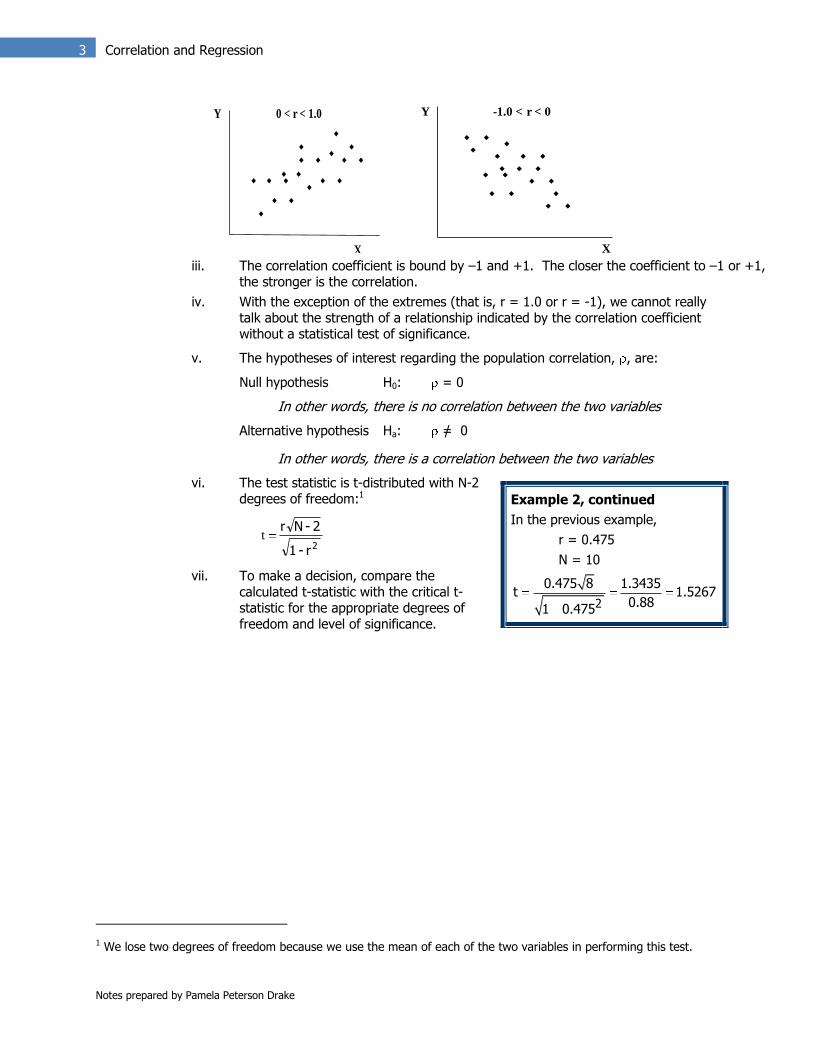
Example 2, continued Consider the following observations on X and Y:

Observation X Y

1 12 50

2 13 54

3 10 48

4 9 47

5 20 70

6 7 20

7 4 15

8 22 40

9 15 35

10 23 37

Sum 135 416 The estimated regression line is:

yi = 25.559 + 1.188 xi

and the residuals are calculated as:

Observation x y y y- y 2

1 12 50 39.82 10.18 103.68

2 13 54 41.01 12.99 168.85

3 10 48 37.44 10.56 111.49

4 9 47 36.25 10.75 115.50

5 20 70 49.32 20.68 427.51

6 7 20 33.88 -13.88 192.55

7 4 15 30.31 -15.31 234.45

8 22 40 51.70 -11.70 136.89

9 15 35 43.38 -8.38 70.26

10 23 37 52.89 -15.89 252.44

Total 0 1,813.63 Therefore,

SSResidaul = 1813.63 / 8 = 226.70 SEE = 226.70 = 15.06

A. The standard error of the estimate helps us gauge the "fit" of the regression line; that is, how well we have described the variation in the dependent variable.

i. The smaller the standard error, the better the fit.

ii. The standard error of the estimate is a measure of close the estimated values (using the estimated regression), the y 's, are to the actual values, the Y's.

iii. The i‟s (a.k.a. the disturbance terms; a.k.a. the residuals) are the vertical

distance between the observed value of Y and that predicted by the equation, the y 's.

iv. The i‟s are in the same terms (unit of measure) as the Y‟s (e.g., dollars, pounds,

billions)

6. The coefficient of determination, R2, is the percentage of variation in the dependent variable (variation of Yi's or the sum of squares total, SST) explained by the independent variable(s).



A. The coefficient of determination is calculated as:

R2= variationTotal

variationExplained

= RegressionTotal Residual

Total Total

SSSS SSTotal variation Unexplained variation

Total variation SS SS

B. An R2 of 0.49 indicates that the independent variables explain 49% of the variation in the dependent variable.

Example 2, continued Continuing the previous regression example, we can calculate the R2:

Observation x y (y- y )2 y Y- y ( y - y )2 2

1 12 50 70.56 39.82 10.18 3.18 103.68

2 13 54 153.76 41.01 12.99 0.35 168.85

3 10 48 40.96 37.44 10.56 17.30 111.49

4 9 47 29.16 36.25 10.75 28.59 115.50

5 20 70 806.56 49.32 20.68 59.65 427.51

6 7 20 466.56 33.88 -13.88 59.65 192.55

7 4 15 707.56 30.31 -15.31 127.43 234.45

8 22 40 2.56 51.70 -11.70 102.01 136.89

9 15 35 43.56 43.38 -8.38 3.18 70.26

10 23 37 21.16 52.89 -15.89 127.43 252.44

Total 416 2,342.40 416.00 0.00 528.77 1,813.63 R2 = 528.77 / 2,342.40 = 22.57% or R2 = 1 – (1,813.63 / 2,342.40) = 1 – 0.7743 = 22.57%

7. A confidence interval is the range of regression coefficient values for a given value estimate of the coefficient and a given level of probability.

A. The confidence interval for a regression coefficient 1b is calculated as:

1bc1 stb

or

11 bc11bc1 stbbstb

where tc is the critical t-value for the selected confidence level. If there are 30 degrees of freedom and a 95% confidence level, tc is 2.042 [taken from a t-table].

B. The interpretation of the confidence interval is that this is an interval that we believe will

include the true parameter (1b

s in the case above) with the specified level of confidence.

8. As the standard error of the estimate (the variability of the data about the regression line) rises, the confidence widens. In other words, the more variable the data, the less confident you will be when you‟re using the regression model to estimate the coefficient.



9. The standard error of the coefficient is the square root of the ratio of the variance of the regression to the variation in the independent variable:

n

1i

2i

2e

b

)x(x

ss

1ˆ

A. Hypothesis testing: an individual explanatory variable

i. To test the hypothesis of the slope coefficient (that is, to see whether the estimated slope is equal to a hypothesized value, b , Ho: b = b1, we calculate

a t-distributed statistic:

tb =

1

1 1

b

b -b

s

ii. The test statistic is t distributed with N k 1 degrees of freedom (number of

observations (N), less the number of independent variables (k), less one).

B. If the t statistic is greater than the critical t value for the appropriate degrees of

freedom, (or less than the critical t value for

a negative slope) we can say that the slope coefficient is different from the hypothesized value, b1.

C. If there is no relation between the dependent and an independent variable, the slope coefficient, b1 would be zero.

X

Y

b0

0

b1 = 0

A zero slope indicates that there is no change in Y for a given change in X A zero slope indicates that there is no relationship between Y and X.

D. To test whether an independent variable explains the variation in the dependent variable, the hypothesis that is tested is whether the slope is zero:

Ho: b1= 0

versus the alternative (what you conclude if you reject the null, Ho):

Ha: b1 =/ 0

This alternative hypothesis is referred to as a two-sided hypothesis. This means that we reject the null if the observed slope is different from zero in either direction (positive or negative).

E. There are hypotheses in economics that refer to the sign of the relation between the dependent and the independent variables. In this case, the alternative is directional (>

Note: The formula for the standard error of the coefficient has the variation of the independent variable in the denominator, not the variance. The variance = variation / n-1.



or <) and the t-test is one-sided (uses only one tail of the t-distribution). In the case of a one-sided alternative, there is only one critical t-value.

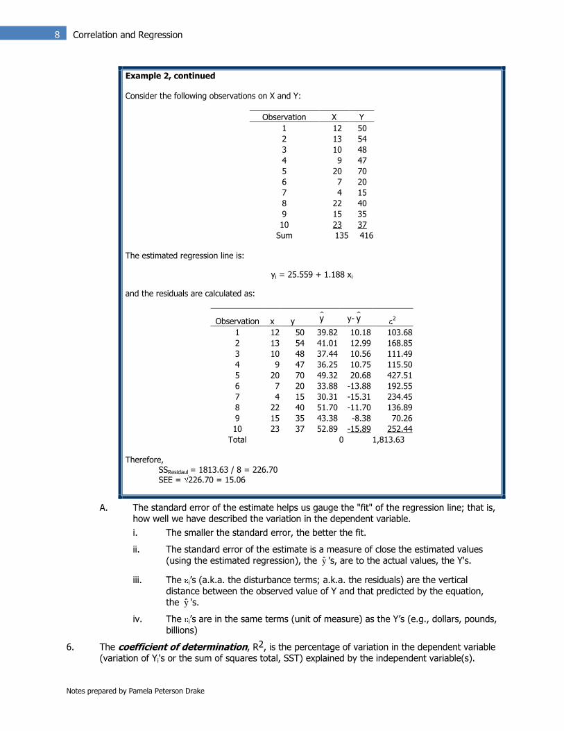
Example 3: Testing the significance of a slope coefficient Suppose the estimated slope coefficient is 0.78, the sample size is 26, the standard error of the

coefficient is 0.32, and the level of significance is 5%. Is the slope difference than zero?

The calculated test statistic is: tb =

1

11 bb

bs

ˆ= 2.4375

0.32

00.78

The critical t-values are 2.060:

-2.060 2.060

____________|_____________________|__________ Reject H0 Fail to reject H0 Reject H0

Therefore, we reject the null hypothesis, concluding that the slope is different from zero.

10. Interpretation of coefficients.

A. The estimated intercept is interpreted as the value of the dependent variable (the Y) if the independent variable (the X) takes on a value of zero.

B. The estimated slope coefficient is interpreted as the change in the dependent variable for a given one-unit change in the independent variable.

C. Any conclusions regarding the importance of an independent variable in explaining a dependent variable requires determining the statistical significance if the slope coefficient. Simply looking at the magnitude of the slope coefficient does not address this issue of the importance of the variable.

11. Forecasting is using regression involves making predictions about the dependent variable based on average relationships observed in the estimated regression.

A. Predicted values are values of the dependent variable based on the estimated regression coefficients and a prediction about the values of the independent variables.

B. For a simple regression, the value of Y is predicted as:

Example 4 Suppose you estimate a regression model with the following estimates:

y = 1.50 + 2.5 X1

In addition, you have forecasted value for the independent variable, X1=20. The forecasted value for y is 51.5:

y = 1.50 + 2.50 (20) = 1.50 + 50 = 51.5



y = i0 bb ˆˆ xp

where y is the predicted value of the dependent variable, and

xp is the predicted value of the independent variable (input).

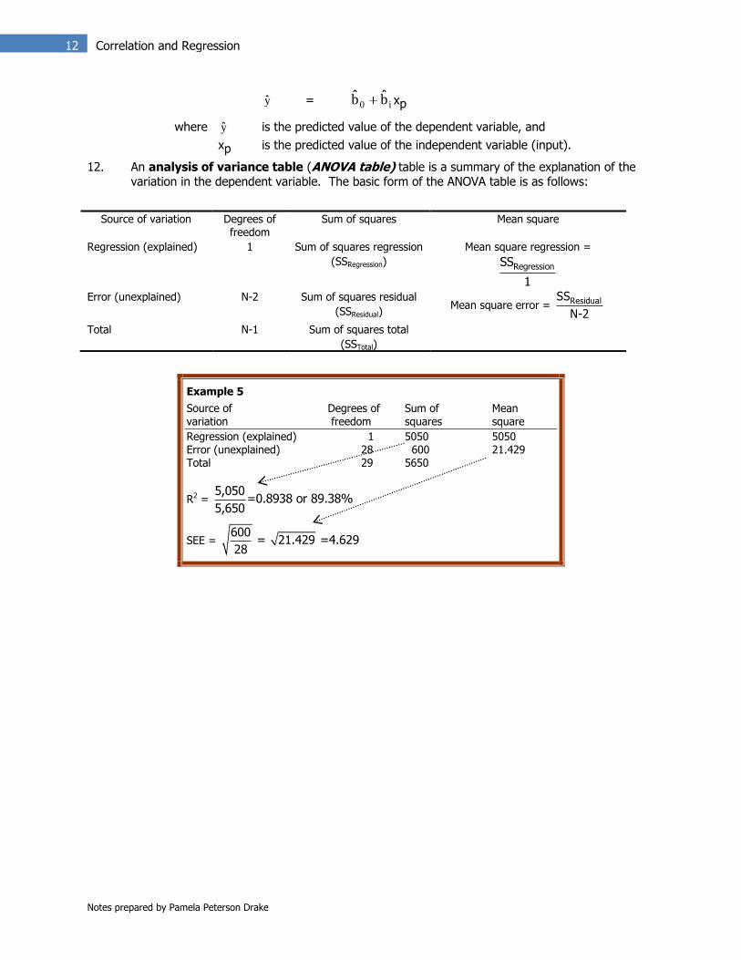
12. An analysis of variance table (ANOVA table) table is a summary of the explanation of the variation in the dependent variable. The basic form of the ANOVA table is as follows:

Source of variation Degrees of freedom

Sum of squares Mean square

Regression (explained) 1 Sum of squares regression

(SSRegression)

Mean square regression =

RegressionSS

1

Error (unexplained) N-2 Sum of squares residual

(SSResidual) Mean square error = ResidualSS

N-2

Total N-1 Sum of squares total

(SSTotal)

Example 5

Source of Degrees of Sum of Mean variation freedom squares square

Regression (explained) 1 5050 5050 Error (unexplained) 28 600 21.429 Total 29 5650

R2 = 5,050

=0.8938 or 89.38%5,650

SEE = 600

= 21.429 =4.62928



Multiple Regression 1. Multiple regression is regression analysis with more than one independent variable.

A. The concept of multiple regression is identical to that of simple regression analysis except that two or more independent variables are used simultaneously to explain variations in the dependent variable.

y = b0 + b1x1 + b2x2 + b3x3 + b4x4

B. In a multiple regression, the goal is to minimize the sum of the squared errors. Each slope coefficient is estimated while holding the other variables constant.

2. The intercept in the regression equation has the same interpretation as it did under the simple linear case – the intercept is the value of the dependent variable when all independent variables are equal zero.

3. The slope coefficient is the parameter that reflects the change in the dependent variable for a one unit change in the independent variable.

A. The slope coefficients (the betas) are described as the movement in the dependent variable for a one unit change in the independent variable – holding all other independent variables constant.

B. For this reason, beta coefficients in a multiple linear regression are sometimes called partial betas or partial regression coefficients.

4. Regression model:

Yi = b0 + b1 x1i + b2 x2i + i

where:

bj is the slope coefficient on the jth independent variable; and

xji is the ith observation on the jth variable.

A. The degrees of freedom for the test of a slope coefficient are N-k-1, where n is the number of observations in the sample and k is the number of independent variables.

B. In multiple regression, the independent variables may be correlated with one another, resulting in less reliable estimates. This problem is referred to as multicollinearity.

5. A confidence interval for a population regression slope in a multiple regression is an interval centered on the estimated slope:

ibciiibci

ibci

stbbstb

or

stb

A. This is the same interval using in simple regression for the interval of a slope coefficient.

B. If this interval contains zero, we conclude that the slope is not statistically different from zero.

6. The assumptions of the multiple regression model are as follows:

We do not represent the multiple regression graphically because it would require graphs that are in more than two dimensions.

A slope by any other name …

The slope coefficient is the elasticity of the dependent variable with respect to the independent variable.

In other words, it‟s the first derivative of the dependent variable with respect to the independent variable.



A. A linear relationship exists between dependent and independent variables.

B. The independent variables are uncorrelated with the residuals; that is, the independent variable is not random. In addition, there is no exact linear relation between two or more independent variables. [Note: this is modified slightly from the assumptions of the simple regression model.]

C. The expected value of the disturbance term is zero; that is, E( i)=0

D. There is a constant variance of the disturbance term; that is, the disturbance or residual terms are all drawn from a distribution with an identical variance. In other words, the disturbance terms are homoskedastistic. [A violation of this is referred to as heteroskedasticity.]

E. The residuals are independently distributed; that is, the residual or disturbance for one observation is not correlated with that of another observation. [A violation of this is referred to as autocorrelation.]

F. The disturbance term (a.k.a. residual, a.k.a. error term) is normally distributed.

G. The residual (a.k.a. disturbance term, a.k.a. error term) is what is not explained by the independent variables.

7. In a regression with two independent variables, the residual for the ith observation is:

i =Yi – ( 0b + 1b x1i + 2b x2i)

8. The standard error of the estimate (SEE) is the standard error of the residual:

se = 1kN

SSE

1kN

ε

SEE

N

1t

2t

ˆ

9. The degrees of freedom, df, are calculated as:

1)(kN1kN1st variableindependen

ofnumber

nsobservatio

ofnumber df

A. The degrees of freedom are the number of independent pieces of information that are used to estimate the regression parameters. In calculating the regression parameters, we use the following pieces of information:

The mean of the dependent variable.

The mean of each of the independent variables.

B. Therefore,

if the regression is a simple regression, we use the two degrees of freedom in estimating the regression line.

if the regression is a multiple regression with four independent variables, we use five degrees of freedom in the estimation of the regression line.

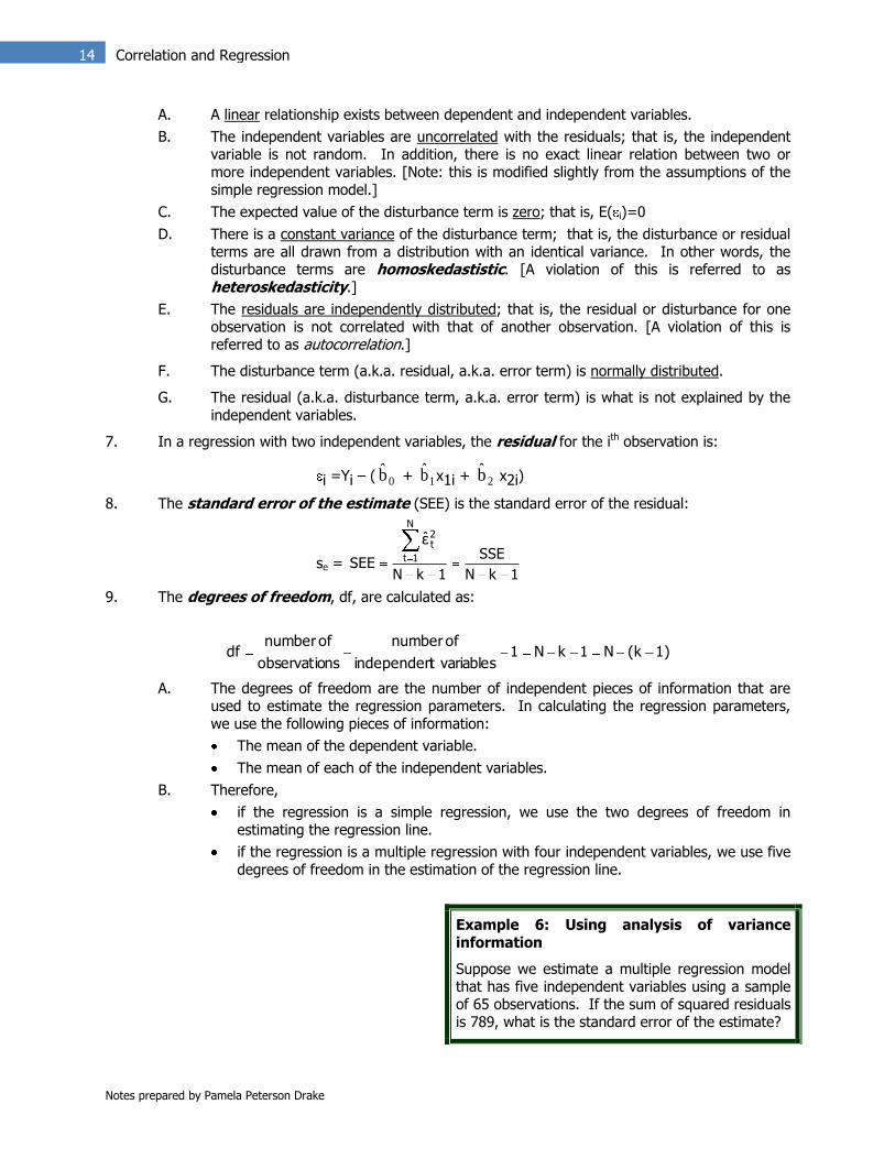
Example 6: Using analysis of variance information

Suppose we estimate a multiple regression model that has five independent variables using a sample of 65 observations. If the sum of squared residuals is 789, what is the standard error of the estimate?



10. Forecasting is using regression involves making predictions about the dependent variable based on average relationships observed in the estimated regression.

A. Predicted values are values of the dependent variable based on the estimated regression coefficients and a prediction about the values of the independent variables.

B. For a simple regression, the value of y is predicted as:

22110 xbxbby ˆˆˆˆˆˆ

where y is the predicted value of the dependent variable,

ib is the estimated parameter, and

ix is the predicted value of the independent variable

C. The better the fit of the regression (that is, the smaller is SEE), the more confident we are in our predictions.

Example 7: Calculating a forecasted value

Suppose you estimate a regression model with the following estimates:

Y = 1.50 + 2.5 X1 0.2 X2 + 1.25 X3

In addition, you have forecasted values for the independent variables:

X1=20 X2=120 X3=50

What is the forecasted value of y?

Solution

The forecasted value for Y is 90:

Y = 1.50 + 2.50 (20) 0.20 (120) + 1.25 (50)

= 1.50 + 50 24 + 62.50 = 90

11. The F-statistic is a measure of how well a set of independent variables, as a group, explain the variation in the dependent variable.

A. The F-statistic is calculated as:

N 2iRegression

i 1

N 2Residual i

i 1

ˆ(y y)SSkMean squared regression MSR kF

SSMean squared error MSE ˆ(y y)N-k-1 N k 1

Solution

Given:

SSResidual = 789

N = 65

k = 5

SEE = 789 789

= =13.37365-5-1 59

Caution: The estimated intercept and all the estimated slopes are used in the prediction of the dependent variable value, even if a slope is not statistically significantly different from zero.



B. The F statistic can be formulated to test all independent variables as a group (the most

common application). For example, if there are four independent variables in the model, the hypotheses are:

H0: 0bbbb 4321

Ha: at least one bi 0

C. The F-statistic can be formulated to test subsets of independent variables (to see whether they have incremental explanatory power). For example if there are four independent variables in the model, a subset could be examined:

H0: 1 4b =b =0

Ha: b1 or b4 0

12. The coefficient of determination, R2, is the percentage of variation in the dependent variable explained by the independent variables.

R2 = variationTotal

variationExplained=

Total Unexplained-

variation variation

Total variation

R2 =

N2

i 1

N2

i 1

ˆ(y y)

(y y)

A. By construction, R2 ranges from 0 to 1.0

B. The adjusted-R2 is an alternative to R2:

)( 22 R1kN

1N1R

i. The adjusted R2 is less than or equal to R2 („equal to‟ only when k=1).

ii. Adding independent variables to the model will increase R2. Adding independent variables to the model may increase or decrease the adjusted-R2 (Note: adjusted-R2 can even be negative).

iii. The adjusted R2 does not have the “clean” explanation of explanatory power that the R2 has.

13. The purpose of the Analysis of Variance (ANOVA) table is to attribute the total variation of the dependent variable to the regression model (the regression source in column 1) and the residuals (the error source from column 1).

A. SSTotal is the total variation of Y about its mean or average value (a.k.a. total sum of squares) and is computed as:

n2

Total i

i=1

SS = (y -y)

where y is the mean of Y.

B. SSResidual (a.k.a. SSE) is the variability that is unexplained by the regression and is computed as:

0 < R2

< 1



n2

Residual i i i

i=1

ˆˆSS =SSE= (y -y ) = ε

where is Y the value of the dependent variable using the regression equation.

C. SSRegression (a.k.a. SSExplained) is the variability that is explained by the regression equation and is computed as SSTotal – SSResidual.

N2

Regression i

i=1

ˆSS = (y -y)

D. MSE is the mean square error, or MSE = SSResidual / (N – k - 1) where k is the number of independent variables in the regression.

E. MSR is the mean square regression, MSR =SSRegression / k

Analysis of Variance Table (ANOVA)

Source

df

(Degrees of Freedom)

SS

(Sum of Squares)

Mean

Square

(SS/df)

Regression k SSRegression MSR

Error N-k-1 SSResidual MSE

Total N-1 SSTotal

Regression2 Residual

Total Total

SS SSR = =1-

SS SS

MSRF=

MSE

14. Dummy variables are qualitative variables that take on a value of zero or one.

A. Most independent variables represent a continuous flow of values. However, sometimes the independent variable is of a binary nature (it‟s either ON or OFF).

B. These types of variables are called dummy variables and the data is assigned a value of "0" or "1". In many cases, you apply the dummy variable concept to quantify the impact of a qualitative variable. A dummy variable is a dichotomous variable; that is, it takes on a value of one or zero.

C. Use one dummy variable less than the number of classes (e.g., if have three classes, use two dummy variables), otherwise you fall into the dummy variable "trap" (perfect multicollinearity – violating assumption [2]).

D. An interactive dummy variable is a dummy variable (0,1) multiplied by a variable to create a new variable. The slope on this new variable tells us the incremental slope.

15. Heteroskedasticity is the situation in which the variance of the residuals is not constant across all observations.

A. An assumption of the regression methodology is that the sample is drawn from the same population, and that the variance of residuals is constant across observations; in other words, the residuals are homoskedastic.



B. Heteroskedasticity is a problem because the estimators do not have the smallest possible variance, and therefore the standard errors of the coefficients would not be correct.

16. Autocorrelation is the situation in which the residual terms are correlated with one another. This occurs frequently in time-series analysis.

A. Autocorrelation usually appears in time series data. If last year‟s earnings were high, this means that this year‟s earnings may have a greater probability of being high than being low. This is an example of positive autocorrelation. When a good year is always followed by a bad year, this is negative autocorrelation.

B. Autocorrelation is a problem because the estimators do not have the smallest possible variance and therefore the standard errors of the coefficients would not be correct.

17. Multicollinearity is the problem of high correlation between or among two or more independent variables.

A. Multicollinearity is a problem because

i. The presence of multicollinearity can cause distortions in the standard error and may lead to problems with significance testing of individual coefficients, and

ii. Estimates are sensitive to changes in the sample observations or the model specification.

B. If there is multicollinearity, we are more likely to conclude a variable is not important.

C. Multicollinearity is likely present to some degree in most economic models. Perfect multicollinearity would prohibit us from estimating the regression parameters. The issue then is really a one of degree.

18. The economic meaning of the results of a regression estimation focuses primarily on the slope coefficients. A. The slope coefficients indicate the change in the dependent variable for a one-unit

change in the independent variable. This slope can than be interpreted as an elasticity measure; that is, the change in one variable corresponding to a change in another variable.

B. It is possible to have statistical significance, yet not have economic significance (e.g., significant abnormal returns associated with an announcement, but these returns are not sufficient to cover transactions costs).



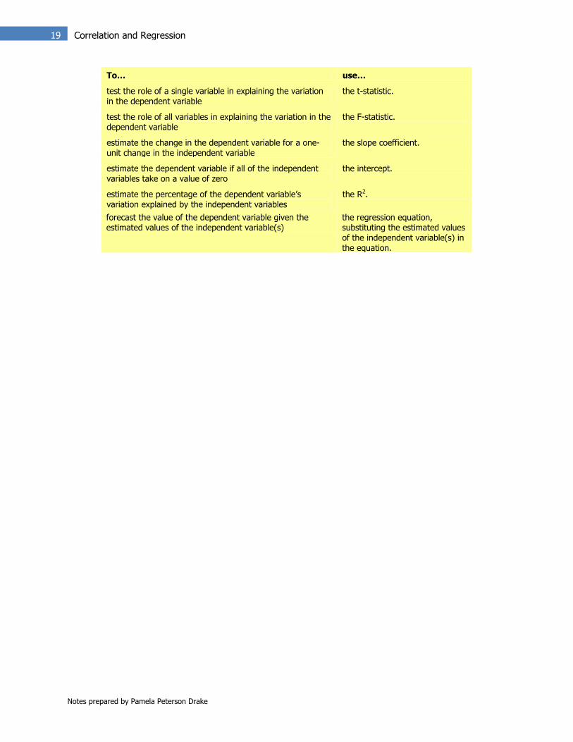
To… use…

test the role of a single variable in explaining the variation in the dependent variable

the t-statistic.

test the role of all variables in explaining the variation in the dependent variable

the F-statistic.

estimate the change in the dependent variable for a one-unit change in the independent variable

the slope coefficient.

estimate the dependent variable if all of the independent variables take on a value of zero

the intercept.

estimate the percentage of the dependent variable‟s variation explained by the independent variables

the R2.

forecast the value of the dependent variable given the estimated values of the independent variable(s)

the regression equation, substituting the estimated values of the independent variable(s) in the equation.



Regression terminology

Analysis of variance

ANOVA

Autocorrelation

Coefficient of determination

Confidence interval

Correlation coefficient

Covariance

Covariation

Cross-sectional

Degrees of freedom

Dependent variable

Explained variable

Explanatory variable

Forecast

F-statistic

Heteroskedasticity

Homoskedasticity

Independent variable

Intercept

Least squares regression

Mean square error

Mean square regression

Multicollinearity

Multiple regression

Negative correlation

Ordinary least squares

Perfect negative correlation

Perfect positive correlation

Positive correlation

Predicted value

R2

Regression

Residual

Scatterplot

se

SEE

Simple regression

Slope

Slope coefficient

Spurious correlation

SSResidual

SSRegression

SSTotal

Standard error of the estimate

Sum of squares error

Sum of squares regression

Sum of squares total

Time-series

t-statistic

Variance

Variation



Regression formulas

Variances

N

1i

2xxVariation

1N

N

1i

2xx

Variance

N

i i

i 1

(x -x)(y -y)

Covariance N-1

Correlation

1N

)y(y

1N

)x(x

)y(y)x(x

rN

1i

2i

N

n1,i

i

N

1i

2i

2i

1N

2r-1

2-Nr t

Regression yi = b0 + b1 xi + i y = b0 + b1x1 + b2x2 + b3x3 + b4x4 + i

1N

)x(x

1N

)x)(xy(y

var(X)

Y)cov(X,b

N

1i

2i

N

1i

ii

1 0 1b =y-b x

Tests and confidence intervals

se 2N

ε

2N

)y(y

2N

xbbyN

1i

2i

2N

1i

ii

N

1i

2

ii0iˆˆˆˆ

n

1i

2i

2e

b

)x(x

ss

1ˆ

tb = 1

1 1

b

b -b

s

N 2iRegression

i 1

N 2Residual i

i 1



11 bc11bc1 stbbstb



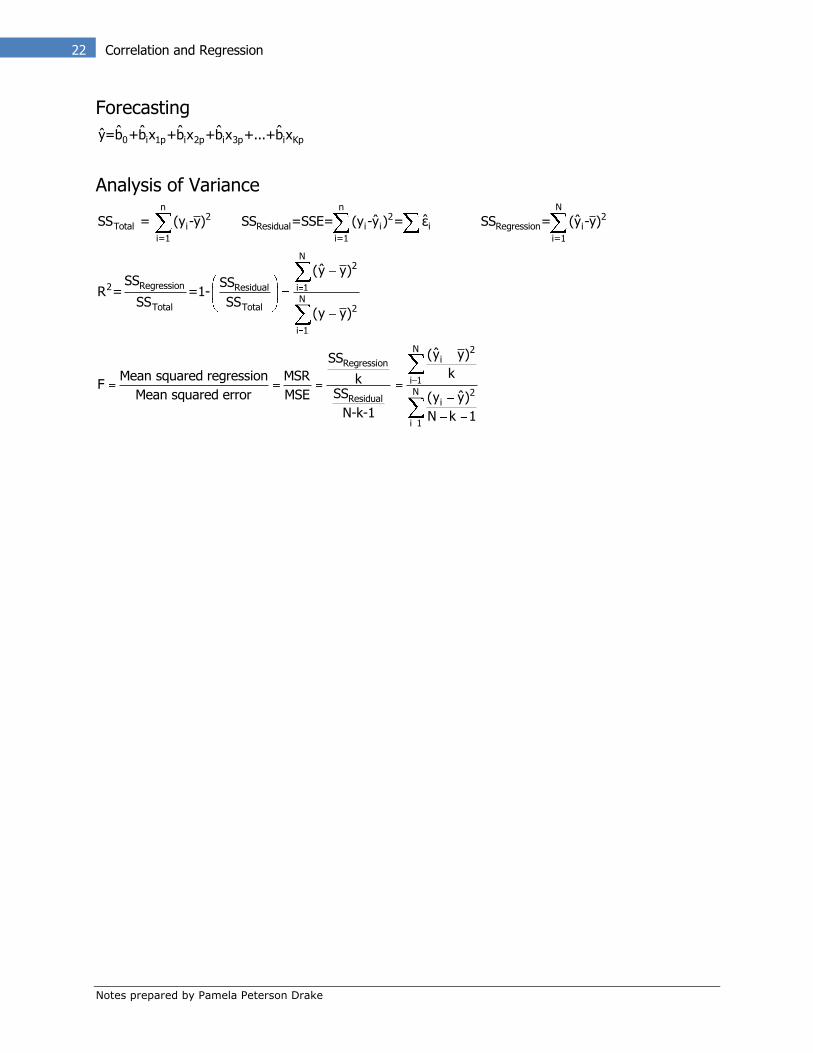
Forecasting

0 i 1p i 2p i 3p i Kpˆ ˆ ˆ ˆ ˆy=b +b x +b x +b x +...+b x

Analysis of Variance n

2Total i

i=1

SS = (y -y) n

2Residual i i i

i=1

ˆˆSS =SSE= (y -y ) = ε N

2Regression i

i=1

ˆSS = (y -y)

N2

Regression2 Residual i 1

NTotal Total 2

i 1

ˆ(y y)SS SS

R = =1-SS SS

(y y)

N 2iRegression

i 1

N 2Residual i

i 1



Documents

Correlation and Regression Notes - educ.jmu.edueduc.jmu.edu/~drakepp/FIN360/readings/Regression_notes.pdf · 5 Correlation and Regression ... Regression is the analysis of the relation