672 u?,tn?TRANSACTIONS ON MICROWAVS THEORY AND TECHNIQUM, VOL. MTr-28, NO. 6, JUNE 1980

J40

J2C

c

-J2C

-J4C

?

112GHZ

10

\

Io 20 40 —

J

60 fl

Fig. 4. Gptirnum source impedance.

agreement with the design objectives. Afterwards, small losses

have been introduced in all transmission-line sections. The

amount of resistive losses is specified by the (unloaded) Q

factors given in parentheses. These values have been arbitrarily

selected within the range of typical Q factors for microstrip

transmission lines. For example, a 504 microstrip etched on a

0.5-mm thick substrate having a relative dielectric constant 2.6

has the Q factor of about 200 at the frequency 1 GHz. The exact

value depends on the conductor thickness, the dielectric losses,

and on the choice of the ground plane material, but these details

are not relevant for the subject of the present paper. By using the

Q factors from Fig. 2 in the computer analysis of the filter, the

attenuation curve is obtained such as shown in Fig. 3 as a

dashed line.

The noise factor F of the lossy filter, terminated by 5041

resistances on both sides, is now computed from (2). The result

is shown in Fig. 3 as a solid line. Unlike the attenuation curve,

the noise factor does not exhibit arty ripple. This is explained by

the fact that the attenuation ripple is caused by the mismatch

mechanism, whereas the noise produced in the filter is caused

solely by the dissipative mechanism.

In order to observe the optimum noise factor which could be

theoretically obtained by the filter at han~ the computed value

FO is also plotted in Fig. 3 (thin line). As can be seen, not much

can be gained by changing the source impedance from the value

50 $2 to ZO, the optimum source impedance. At the center

frequency the improvement would be only 0.03 dB, and at the

edge of the passband the improvement would reach 0.6 dB.

The computed source impedance 20 which is needed for

achieving the optimum noise factor is shown in Fig. 4 as a

function of frequency. As frequency increases, the locus of ZO

moves counterclockwise on the complex plane. Since the

driving-point impedance of any passive network exhibits a clock-

wise rotation with increasing frequency, an exact synthesis of a

passive matching network for achieving the required ZO at all

frequencies is impossible. However, the optimum match could

be achieved at any particular frequency of interest.

In conclusion, it has been shown how existing computer

programs for the analysis of cascaded two-ports can be supple-

mented to include the noise analysis of lossy microwave filters.

Such a numerical analysis shows that, within the passbanh the

noise factor of a passive integrated-circuit microwave filter is

only slightly lower than the attenuation. No significant improve-

ment in the noise factor of the filter can be achieved by an

intentional mismatch of the source impedance to its optimum

value.

[1]

[2]

[3]

[4]

[5]

[6]

[7]

[s]

[9]

mFERENCES

F’. E. Green, “General purpose programs for the frequency domainanalysis of microwave circuits,” IEEE Trans. Microwaos Theory Tech.,vol. MTT- 17, pp. 506-514, Aug. 1969.W. N. Parker, “DIPNET: A general distributed parameter networkanalysis program,” IEEE Trans. Microwave Theory Tech., vol. MT’T- 17,pp. 495–505, Aug. 1969.T. C. Ciseo, “Desi~ of microwave components by computer,”’ Rep.NASA CR- 1982, Mar. 1972.B. S. Perbm and V. G. Gelnovatch, “Computer aided design, sinmla-tion and optimization,” in Adoartces in Microwaves, vol. 8, L. Young andH. Sobol, Eds., New York: Academic, 1974.J. F. White, Semiconductor Control. Burlington, MA: Artech, 1977, ch.VI.M. Hillbum, “Learn a new format, and analyze complex networks~Microwaczes, pp. 82–91, Feb. 1979.H. A. Haus and R. B. Adler, Circuit Theory of Linear Noi~ Networks.New York: Wiley, 1959, sec. 3.3.H. Rothe and W. Drddke, “Theory of noisy fourpoles,” Proc. IRE, vol.44, pp. S11–81S, Jnne 1956.H. A. Hau.s, ‘W@ standards on methods of measuring noise in lineartwoports, 1959; Proc. IRE, vol. 48, pp. 60–68, Jan. 1960.

Letters _

Correction to “The Design of Coupled MicrostripLines”

RASHID M. OSMANI

In the above paper,] the authors have described a new proce-

dure for the design of coupled microstrip lines. For the even-

mode case, their results differ from those of Bryant and Weiss [1]

by as much as 14 percent. This is because the authors have used

Manuscript received November 14, 1979.The author is with Defence Electronics Research Laboratory,

Chandrayangutta Lines, Hyderabad 5C0 005, India.1Sina Aktarzad et aI., “The design of coupled microstrip lines,” IEEE

Trans. Microwave Theory Tech., vol. MTT’-23, pp. 4S6–492, June 1975.

Wheeler’s formula for W/H >1 even for the cases when W/H

<1. Using the nomenclature of the referenced paper,’ a cor-

rected procedure for synthesis and analysis is given below.

Synthesis: To calculate W/H and S/H for given Zw and Zw.

( W/H)~g and ( W/H),O corresponding to the impedances ZJ2

and Zm/2 are calculated by using the formulas given in [2].

If ( W/H), <1

( W/H), =8.0

antilog. (ZO/K1 + KJ

K,=84.78

Kz = ~(0,226+0.121/er).(e, +l)’i’ ,

(la)

0018-9480/80/0600-0672$00.75 01980 IEEE

ff3SS TRANSACTIONS ON MfCROWAVE THSORY AND 173CRNfQURS,VOL. MTr-28, NO. 6, JUNR 1980 673

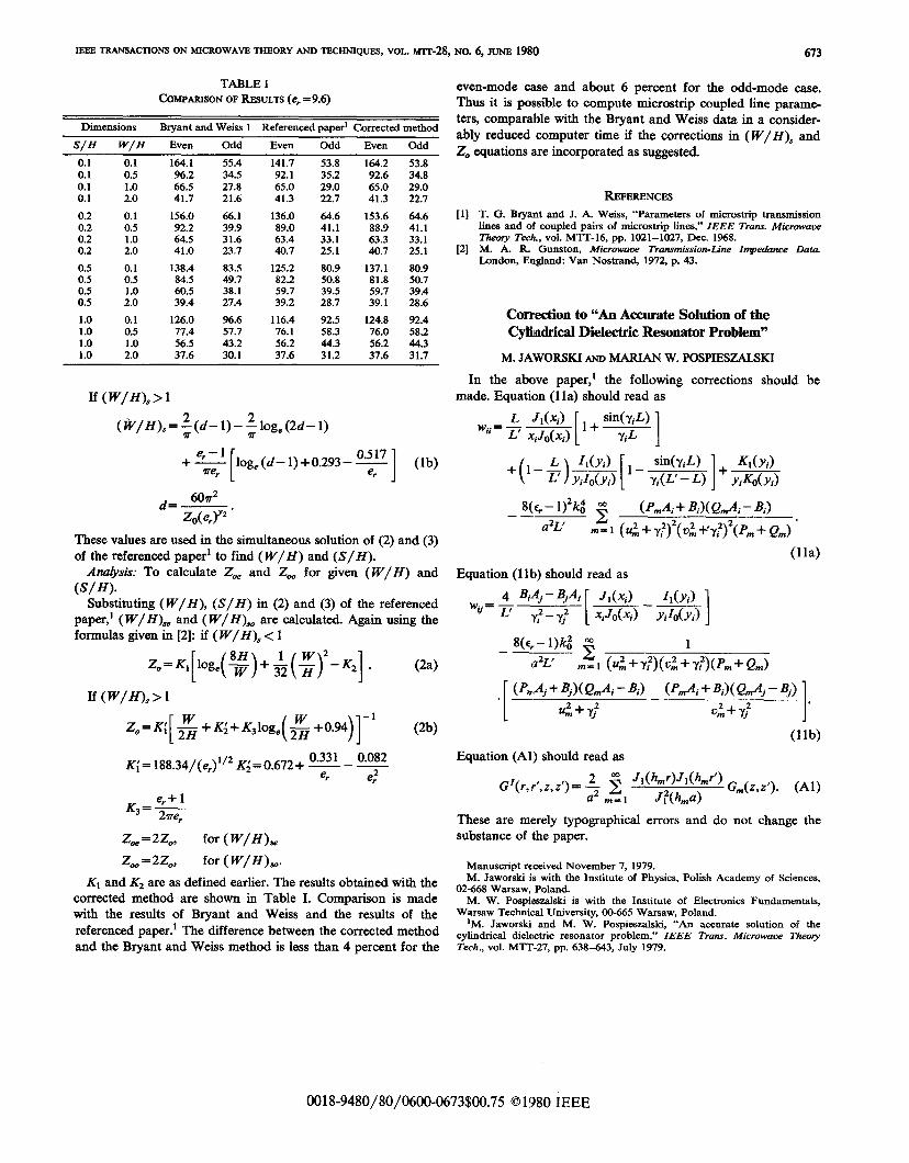
TABLE I

COMPARISON OF Rf3SULTS (e, =9,6)

Dimensions Bryant and Weiss 1 Referenced paperl Corrected method

S/H W/Ii Even Odd Even Odd Even Odd

0.1 0.1 164.1 55.4 141.7 53.8 164.2 53.80.1 0.5 96.2 34.5 92.1 35.2 92.6 34.80.1 1.0 66.5 27.8 65.0 29.0 65.0 29.00.1 2.0 41.7 21.6 41.3 22.7 41.3 22.7

0.2 0.1 156.0 66.1 136.0 64.6 153.6 64.60.2 0.5 92.2 39.9 89.0 41.1 88.9 41.10.2 1.0 64.5 31.6 63.4 33.1 63.3 33.10.2 2.0 41.0 23.7 40.7 25.1 40.7 25.1

0.5 0.1 138.4 83.5 125.2 80.9 137.1 80.90.5 0.5 84.5 49.7 82.2 50.8 81.8 50.70.5 1.0 60.5 38.1 59.7 39.5 59.7 39.40.5 2.0 39.4 27.4 39.2 28.7 39.1 28.6

1.0 0.1 126.0 96.6 116.4 92.5 124.8 92.41.0 0.5 77.4 57.7 76.1 58.3 76.0 58.21.0 1.0 56.5 43.2 56.2 44.3 56.2 44.31.0 2.0 37.6 30.1 37.6 31.2 37.6 31.7

If ( W/H), >1

(i’V/H).= :(d– 1)- ; loge(2d– 1)

e++

[loge (d– 1) +0.293 – ~

wer 1(lb)r

~= 607r2

*“

These values are used in the simultaneous solution of (2) and (3)

of the referenced paper* to find ( W/H) and (LS/H).

Ana&sis: To calculate Z* and Zw for given (W/H) and

(S/H).

Substituting (W/H), (S/H) in (2) and (3) of the referenced

paper,] ( W/H)*e and ( W/H)$O are calculated. Again using the

formulas given in [2]: if ( W/H), <1

zo=K1[loge(y)+&(gp2].

If (W/H)=> 1

[ (ZO=K; ~+ K;+ K310ge &+O.94

)]

–1

0.331 0.082K;= 188.34/(e,)112 K.j= 0.672+ ~ – —

r e:

er+lK3=~

~= 2Z0,z for (W/H),.

Zm = 22., for ( W/H).o.

(2a)

(2b)

K, and K2 are as defined earlier. The results obtained with the

corrected method are shown in Table I. Comparison is made

with the results of Bryant and Weiss and the results of the

referenced paper.1 The difference between the corrected method

and the Bryant and Weiss method is less than 4 percent for the

even-mode case and about 6 percent for the odd-mode case.

Thus it is possible to compute microstrip coupled line parame-

ters, comparable with the Bryant and Weiss data in a consider-

ably reduced computer time if the corrections in (W/H), and

ZO equations are incorporated as suggested.

R5Ff3rt5Ncf3s

[1] T. G. Bryant and J. A. Weiss, “Parameters of rnicrostrip transmissionlines and of coupled pairs of rnicrostrip lines,” IEEE Trans. A4icrowaceTheory Tech., vol. M’lT-16, pp. 1021–1027, Dec. 1%8.

[2] M. A. R. Gunston, Microwave Transmission.Lirte Impeairnce Data.London, England: Van Nostrand, 1972, p. 43.

Correction to “An Accnrate Solution of the

Cylincbkal Dlektric Resonator Problem”

M. JAWORSKI AND MARL4N W. POSPIESZALSKI

In the above paper,l the following corrections should be

made. Equation (1 la) should read as

“’==-[l+W+(+i%[R2!’Yq’-

8(%– l)2k$ ~x

(P-A,+ Bi)(QmAi - B,).—

a2L’ ~= 1 (u;+ y;)2(u;+’y;)2(~m + Qm) “

(ha)

Equation (1 lb) should read as

[

4 BjAj – BjAi J](xi) Z,(yi)

‘~=ry;-y;— -—xiJO(xi) YizO(Yi) 1

8(c,– l)k; m— ——

az~ &I (u;+ Y;)(o;:Y?)(%+ Qnr)

[

(~m~j+ ~)(QmAi – ~i) (l’mAi + Bi)(Qm~j– Bj)._ —

u:+ ~? v:+ yj 1“(llb)

Equation (Al) should read as

~ J1(hmr)J1(h#)G1(r, r’,z, z’) = ; ~

Jf(ltma)Gm(z,z’). (Al)

a ~=1

These are merely typographical errors and do not change the

substance of the paper.

Manuscript received November 7, 1979.M. Jaworski is with the Institute of Physics, Polish Academy of Sciences,

02-668 Warsaw, Poland.M. W. Pospieszalski is with the Institute of Electronics Fundamentals,

Warsaw Teclrnkd University, 0@665 Warsaw, Poland.1M. Jaworski and M. W. Pospieszalski, “An accurate solution of the

cylindrical diek:ctric resonator problem,” IEEE Trans. Microwaoe TheotyTech., vol. MTT-27, pp. 638–643, Jrdy 1979.

0018-9480/80/0600-0673$00.75 @1980 IEEE