NTIA Technical Memorandum 10-464

CORRECTION FACTORS AND MEASUREMENT PROCEDURE TO

ASSESS THE INTERFERENCE IMPACT OF LINEAR SWEPT FREQUENCY SIGNALS ON

RADIO RECEIVERS

technical memorandum series

U.S. DEPARTMENT OF COMMERCE National Telecommunications and Information Administration

NTIA Technical Memorandum 10-464

CORRECTION FACTORS AND MEASUREMENT PROCEDURE TO

ASSESS THE INTERFERENCE IMPACT OF LINEAR SWEPT

FREQUENCY SIGNALS ON RADIO RECEIVERS

Edward F. Drocella

David S. Anderson

U.S. DEPARTMENT OF COMMERCE

Gary Locke, Secretary

Lawrence E. Strickling Assistant Secretary for Communications and Information

December 2009

ii

ACKNOWLEDGMENTS

The authors wish to thank Brent Bedford of the National Telecommunications and Infor-

mation Administration’s Institute for Telecommunication Sciences, for his support and work in

performing the measurements that were fundamental to the completion of this technical memo-

randum.

iii

EXECUTIVE SUMMARY

The National Telecommunications and Information Administration (NTIA) is developing

a handbook documenting the best practices in spectrum engineering. This technical memoran-

dum provides a methodology to determine the average and peak power level at the output of a

filter with a linear swept frequency pulse train input to the filter. Using this method, NTIA cal-

culated two correction factors necessary to accurately compute the interference power level of a

system that employs linear swept frequency signals. The two correction factors enable the con-

version of the peak power at the filter input to the peak power or average power at the output.

These correction factors cover the case where the peak input power is stated in dB relative to a

reference power (e.g., dBW). NTIA also carried out, as part of this technical memorandum,

measurements of linear swept frequency signals at the input and output of a variety of filter

bandwidths. A comparison of measured and calculated correction factors showed the values to

be in good agreement. The measurements carried out in this technical memorandum resulted in

the development of a general procedure for measuring the emissions of a system employing li-

near swept frequency techniques. This method enables an accurate measurement of the emis-

sions from which to assess compatibility with other radio services. The correction factors and

the measurement procedure described in this technical memorandum will be used in the devel-

opment of the Best Practices Handbook.

iv

TABLE OF CONTENTS

EXECUTIVE SUMMARY ..................................................................................................... iii

TABLE OF CONTENTS ......................................................................................................... iv

GLOSSARY OF ACRONYMS AND

ABBREVIATIONS ................................................................................................................... v

SECTION 1.0 INTRODUCTION ........................................................................................ 1-1

1.1 BACKGROUND .................................................................................................. 1-1

1.2 OBJECTIVE ......................................................................................................... 1-3

1.3 APPROACH ......................................................................................................... 1-3

SECTION 2.0 ANALYTICAL APPROACH ....................................................................... 2-1

2.1 INTRODUCTION ................................................................................................. 2-1

2.2 PEAK POWER CORRECTION FACTOR ........................................................... 2-1

2.3 AVERAGE POWER CORRECTION FACTOR .................................................... 2-2

SECTION 3.0 ANALYSIS OF MEASUREMENTS ........................................................... 3-1

3.1 DESCRIPTION OF MEASUREMENTS ............................................................. 3-1

3.2 DISCUSSION OF MEASUREMENTS .………………………………………….. 3-1

3.2.1 Peak Power Measurements ..................................................................... 3-1

3.2.2 Average Power Measurements ................................................................ 3-4

3.2.3 Applications of Linear Swept Frequency Correction Factors ................... 3-8

SECTION 4.0 GENERAL MEASUREMENT PROCEDURE FOR LINEAR

SWEPT FREQUENCY SIGNALS.…………...…………….………….………….………....4-1

4.1 GENERAL MEASUREMENT PROCEDURE ..................................................... 4-1

4.2 DESCRIPTION OF GENERAL MEASUREMENT PROCEDURE ..................... 4-1

SECTION 5.0 CONCLUSIONS .……………………………………………...……………...5-1

5.1 CONCLUSIONS .................................................................................................. 5-1

v

GLOSSARY OF ACRONYMS AND ABBREVIATIONS

AWG Arbitrary Waveform Generator

Bt Extent of Frequency Sweep

BW Bandwidth

BWCF Bandwidth Correction Factor

BW3dB 3 dB Filter Bandwidth

CFA Average Power Correction Factor

CFP Peak Power Correction Factor

EIRP Equivalent Isotropically Radiated Power

IF Intermediate Frequency

ITS Institute for Telecommunication Sciences

kHz Kilohertz

LNA Low Noise Amplifier

MHz Megahertz

msec Millisecond

NTIA National Telecommunications and Information Administration

OSM Office of Spectrum Management

PAO Average Power at the Output of Filter

PPi Peak Power at the Input of Filter

PPO Peak Power at the Output of Filter

PRT Pulse Repetition Time

PW Pulse Width

RBW Resolution Bandwidth

RF Radio Frequency

RMS Root Mean Square

SR Sweep Rate

τi Input Pulse Width

UFS Unit Under Test Frequency Sweep

UUT Unit Under Test

µsec Microsecond

1-1

SECTION 1.0

INTRODUCTION

1.1 BACKGROUND

The National Telecommunications and Information Administration (NTIA) Of-

fice of Spectrum Management is examining best practices in spectrum management for

use by regulators, technology developers, manufacturers and service providers. This ef-

fort includes the development of a Best Practices Handbook that will aggregate a com-

mon set of approaches for conducting engineering analyses and will assemble a common

set of criteria for performing technical studies to evaluate emerging technologies. NTIA

will prepare a series of technical memorandums on various topics related to performing

engineering analyses and will use the results of the individual technical memorandums to

develop the Best Practices Handbook. This technical memorandum is one in a series ad-

dressing specific topics related to spectrum engineering.

An increasing number of federal and non-federal systems being developed em-

ploy linear swept frequency techniques. For compliance purposes the emissions from

these devices are typically measured in a reference bandwidth (e.g., 1 MHz). To assess

the compatibility of systems employing linear swept frequency techniques with other ra-

dio receivers, both average and peak power levels at the victim receiver intermediate fre-

quency output are required. To perform this assessment, it is necessary to develop a

means of converting the power (peak or average) of a linear swept frequency signal as

measured in one bandwidth (e.g., reference bandwidth) to what would be expected in

another bandwidth (victim receiver bandwidth). To perform this conversion, equations

referred to as correction factors can be developed. In addition to providing a conversion

for determining the peak or average power in different bandwidths, the correction factor

can also be used to convert between peak and average power levels within the same

bandwidth.

1.2 OBJECTIVE

The objective of the measurements and analyses described in this technical me-

morandum is to develop peak and average power correction factors for linear swept fre-

quency signals. To accomplish this objective, NTIA conducted a series of tests providing

measured data to support the understanding of the signal at the output of a filter over a

range of filter bandwidths that results from each of a variety of input linear swept fre-

quency signals. The measurements carried out in this technical memorandum will be

used to develop a general procedure for measuring the emissions of a system employing

linear swept frequency techniques.

1.3 APPROACH

The NTIA Institute for Telecommunication Sciences (ITS), in conjunction with

the NTIA Office of Spectrum Management, performed the measurements described in

this technical memorandum.

1-2

During the initial phase of the program, NTIA developed a linear swept frequency

signal source. The swept frequency signal source was capable of generating a constant

amplitude signal that swept across a range of at least 15 MHz with sweep rates of 0.005,

0.05, 0.5, 5, 50 and 500 kHz per microsecond (µsec). The carrier frequency was not a

critical parameter in this measurement program.

The swept frequency signals were input to a spectrum analyzer. With the spec-

trum analyzer in a zero span mode at a frequency that is at the mid-point of the 15 MHz

sweep range of the swept frequency signal generator, signals were measured in the spec-

trum analyzer with resolution bandwidths (RBWs) of 3 MHz, 1MHz, 300 kHz, 100 kHz,

30 kHz, and 10 kHz for each of the sweep rates.

The signal was measured using the root-mean-square (RMS) average and peak

detectors. The peak and average power levels were measured using the maximum hold

feature of the spectrum analyzer for approximately ten scans of the source signal. These

multiple scans were performed for each of the sweep rates. The average power using the

RMS average detector was measured over a 1 millisecond (msec) time interval. The peak

power for each input signal was obtained.

In addition, similar spectrum analyzer measurements of peak and average power

were carried out with the swept frequency held constant at 500 kHz/µsec and the pulse

repetition time varied (600 µsec, 1.1 msec, and 6 msec). These additional measurements

show the impact of duty cycle on the average power.

NTIA then analyzed the measured data along with certain analytical representa-

tions to develop a methodology to convert the peak power at a filter input to the peak or

average power at the filter output.

2-1

SECTION 2.0

ANALYTICAL APPROACH

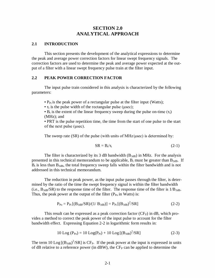
2.1 INTRODUCTION

This section presents the development of the analytical expressions to determine

the peak and average power correction factors for linear swept frequency signals. The

correction factors are used to determine the peak and average power expected at the out-

put of a filter with a linear swept frequency pulse train at the filter input.

2.2 PEAK POWER CORRECTION FACTOR

The input pulse train considered in this analysis is characterized by the following

parameters:

▪ PPi is the peak power of a rectangular pulse at the filter input (Watts);

▪ τt is the pulse width of the rectangular pulse (μsec);

▪ Bt is the extent of the linear frequency sweep during the pulse on-time (τt)

(MHz); and

▪ PRT is the pulse repetition time, the time from the start of one pulse to the start

of the next pulse (μsec).

The sweep rate (SR) of the pulse (with units of MHz/μsec) is determined by:

SR = Bt/τt (2-1)

The filter is characterized by its 3 dB bandwidth (B3dB) in MHz. For the analysis

presented in this technical memorandum to be applicable, Bt must be greater than B3dB. If

Bt is less than B3dB, the total frequency sweep falls within the filter bandwidth and is not

addressed in this technical memorandum.

The reduction in peak power, as the input pulse passes through the filter, is deter-

mined by the ratio of the time the swept frequency signal is within the filter bandwidth

(i.e., B3dB/SR) to the response time of the filter. The response time of the filter is 1/B3dB.

Thus, the peak power at the output of the filter (PPo in Watts) is:

PPo = PPi [(B3dB/SR)/(1/ B3dB)] = PPi [(B3dB)2/SR] (2-2)

This result can be expressed as a peak correction factor (CFP) in dB, which pro-

vides a method to correct the peak power of the input pulse to account for the filter

bandwidth effect. Expressing Equation 2-2 in logarithmic form results in:

10 Log (PPo) = 10 Log(PPi) + 10 Log [(B3dB)2/SR] (2-3)

The term 10 Log [(B3dB)2/SR] is CFP. If the peak power at the input is expressed in units

of dB relative to a reference power (in dBW), the CFP can be applied to determine the

2-2

output in the same power units. There is, however, a limit on the range of applicability of

CFP = 10 Log [(B3dB)2/SR]. The peak correction factor cannot exceed 0 dB or (B3dB)

2/SR

cannot exceed one. That is, if (B3dB)2/SR is greater than one, it should be set equal to one

to determine CFP. If CFP where allowed to have a value greater than 0 dB, the peak pow-

er out of the filter would be greater than the peak power into the filter, which is not poss-

ible.

2.3 AVERAGE POWER CORRECTION FACTOR

Once the peak power at the output of the filter has been determined, the average

power at the output (PAo in Watts) of the filter can be determined by taking into account

the duty cycle of the output pulse train:

PAo= PPo (τo/PRT) (2-4)

where τo is the pulse length at the filter output. This is also the response time of the filter:

τo = 1/B3dB (2-5)

Combining Equations 2-2 and 2-4 results in:

PAo= PPi [(B3dB)2/SR] [1/(B3dB x PRT)] = PPi [B3dB/(SR x PRT)] (2-6)

This produces a correction factor (in logarithmic form) for average power (CFA)

in the same units as that of the peak power (e.g., dBW or dBm):

CFA = 10 Log [B3dB/(SR x PRT)] (2-7)

3-1

SECTION 3.0

ANALYSIS OF MEASUREMENTS

3.1 DESCRIPTION OF MEASUREMENTS

In order to confirm the analytical results presented in Section 2, NTIA ITS per-

formed a series of measurements. The measurements initially involved configuring a

signal generator to linearly sweep from 92.5 to 107.5 MHz. The linearity of the sweep

was confirmed using a vector signal analyzer. The slowest sweep rate used was 5

Hz/µsec and the fastest was 500 kHz/µsec. NTIA ITS used a spectrum analyzer to meas-

ure the peak and average power at the output of the RBW filter. These RBW filters are

incorporated in the spectrum analyzer and have a Gaussian selectivity characteristic. The

average power measurements were made using a RMS detector with an integration time

of 1 msec for the initial measurements.

The pulse-on time of the pulse train was established by the sweep rate selected for

the specific measurement and the extent of the frequency sweep (92.5 to 107.5 MHz).

The off-time between pulses was very short initially such that the difference between to-

tal peak and average power at the filter input was less than 3 dB. The spectrum analyzer

was operated in the zero-span mode with maximum hold and tuned to the center frequen-

cy of the frequency sweep of the pulse.

3.2 DISCUSSION OF MEASUREMENTS

3.2.1 Peak Power Measurements

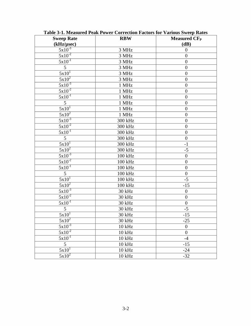
Table 3-1 provides a summary of the peak power measurement results. As shown

in Table 3-1, the measured peak power at the output of the RBW filter relative to the in-

put of the filter is a function of the bandwidth and sweep rate. The quantity measured is

the difference between maximum peak power at the filter input and the measured peak

power at the filter output for a combination of sweep rate and filter bandwidths, CFP = 10

Log [(B3dB)2/SR].

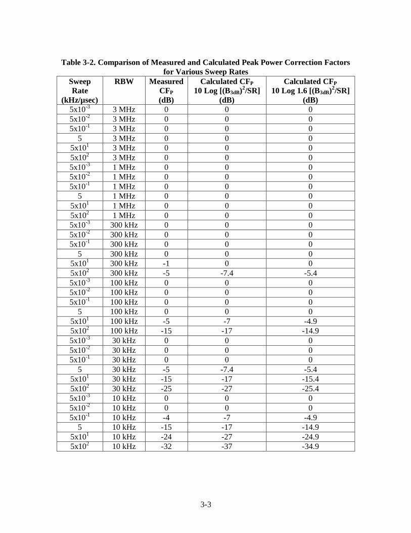
Table 3-2 shows a comparison of measured and calculated CFP values. As shown

in Table 3-2, the calculated CFP values are higher in magnitude than the measured CFP

values. This indicates that the analytical expression developed in Section 2 provides an

overestimate of the actual CFP. Thus, it is necessary to modify the equation for CFP de-

veloped in Section 2. Including a factor of 1.6 in Equation 2-3 results in CFP values in

better agreement with the measurements as shown in the last column in Table 3-2.

3-2

Table 3-1. Measured Peak Power Correction Factors for Various Sweep Rates

Sweep Rate

(kHz/µsec)

RBW Measured CFP

(dB)

5x10-3

3 MHz 0

5x10-2

3 MHz 0

5x10-1

3 MHz 0

5 3 MHz 0

5x101 3 MHz 0

5x102 3 MHz 0

5x10-3

1 MHz 0

5x10-2

1 MHz 0

5x10-1

1 MHz 0

5 1 MHz 0

5x101 1 MHz 0

5x102 1 MHz 0

5x10-3

300 kHz 0

5x10-2

300 kHz 0

5x10-1

300 kHz 0

5 300 kHz 0

5x101 300 kHz -1

5x102 300 kHz -5

5x10-3

100 kHz 0

5x10-2

100 kHz 0

5x10-1

100 kHz 0

5 100 kHz 0

5x101 100 kHz -5

5x102 100 kHz -15

5x10-3

30 kHz 0

5x10-2

30 kHz 0

5x10-1

30 kHz 0

5 30 kHz -5

5x101 30 kHz -15

5x102 30 kHz -25

5x10-3

10 kHz 0

5x10-2

10 kHz 0

5x10-1

10 kHz -4

5 10 kHz -15

5x101 10 kHz -24

5x102 10 kHz -32

3-3

Table 3-2. Comparison of Measured and Calculated Peak Power Correction Factors

for Various Sweep Rates

Sweep

Rate

(kHz/µsec)

RBW Measured

CFP

(dB)

Calculated CFP

10 Log [(B3dB)2/SR]

(dB)

Calculated CFP

10 Log 1.6 [(B3dB)2/SR]

(dB)

5x10-3

3 MHz 0 0 0

5x10-2

3 MHz 0 0 0

5x10-1

3 MHz 0 0 0

5 3 MHz 0 0 0

5x101 3 MHz 0 0 0

5x102 3 MHz 0 0 0

5x10-3

1 MHz 0 0 0

5x10-2

1 MHz 0 0 0

5x10-1

1 MHz 0 0 0

5 1 MHz 0 0 0

5x101 1 MHz 0 0 0

5x102 1 MHz 0 0 0

5x10-3

300 kHz 0 0 0

5x10-2

300 kHz 0 0 0

5x10-1

300 kHz 0 0 0

5 300 kHz 0 0 0

5x101 300 kHz -1 0 0

5x102 300 kHz -5 -7.4 -5.4

5x10-3

100 kHz 0 0 0

5x10-2

100 kHz 0 0 0

5x10-1

100 kHz 0 0 0

5 100 kHz 0 0 0

5x101 100 kHz -5 -7 -4.9

5x102 100 kHz -15 -17 -14.9

5x10-3

30 kHz 0 0 0

5x10-2

30 kHz 0 0 0

5x10-1

30 kHz 0 0 0

5 30 kHz -5 -7.4 -5.4

5x101 30 kHz -15 -17 -15.4

5x102 30 kHz -25 -27 -25.4

5x10-3

10 kHz 0 0 0

5x10-2

10 kHz 0 0 0

5x10-1

10 kHz -4 -7 -4.9

5 10 kHz -15 -17 -14.9

5x101 10 kHz -24 -27 -24.9

5x102 10 kHz -32 -37 -34.9

3-4

NTIA ITS carried out additional peak power measurements with the sweep rate

held constant at 500 kHz/µsec and the PRT varied (600 µsec, 1.1 msec, and 6 msec). The

data set previously discussed included data for a sweep rate of 500 kHz/ µsec and a PRT

of 60 µsec. Table 3-3 shows these data sets and peak power correction factors. As

shown in Table 3-3, the peak power correction is not dependent on the PRT.

Table 3-3. Comparison of Measured and Calculated Peak Power Correction Factors

(Sweep Rate of 500 kHz/600 µsec)

Spectrum

Analyzer

RBW

PRT

Measured

CFP

(dB)

Calculated CFP

10 Log [(B3dB)2/SR]

(dB)

Calculated CFP

10 Log 1.6 [(B3dB)2/SR]

(dB)

3 MHz 60 µsec 0 0 0

3 MHz 600 µsec 0 0 0

3 MHz 1.1 msec 1 0 0

3 MHz 6 msec 1 0 0

1 MHz 60 µsec 0 0 0

1 MHz 600 µsec 0 0 0

1 MHz 1.1 msec 0 0 0

1 MHz 6 msec 0 0 0

300 kHz 60 µsec -5 -7.4 -5.4

300 kHz 600 µsec -5 -7.4 -5.4

300 kHz 1.1 msec -5 -7.4 -5.4

300 kHz 6 msec -5 -7.4 -5.4

100 kHz 60 µsec -15 -17 -14.9

100 kHz 600 µsec -14 -17 -14.9

100 kHz 1.1 msec -14 -17 -14.9

100 kHz 6 msec -14 -17 -14.9

30 kHz 60 µsec -25 -27.4 -25.4

30 kHz 600 µsec -25 -27.4 -25.4

30 kHz 1.1 msec -24 -27.4 -25.4

30 kHz 6 msec -24 -27.4 -25.4

10 kHz 60 µsec -32 -37 -34.9

10 kHz 600 µsec -34 -37 -34.9

10 kHz 1.1 msec -34 -37 -34.9

10 kHz 6 msec -34 -37 -34.9

3.2.2 Average Power Measurements

Table 3-4 provides a summary of the average power measurement results. The

table shows that the measured average power at the output of the RBW filter relative to

the peak power at the filter input as a function of RBW and sweep rate. The quantity of

interest is CFA = 10 Log [B3dB/(SR x PRT)], which is the difference between the peak

power at the input of the filter and the average power at the output. However, this formu-

la for CFA assumes the integration time for the average power measurement is long

enough to include at least one full pulse repetition period at the filter output. If a full

3-5

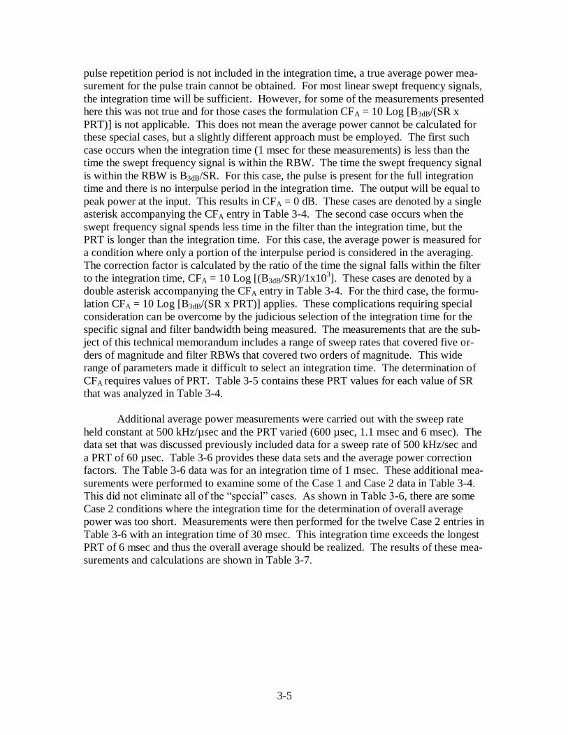
pulse repetition period is not included in the integration time, a true average power mea-

surement for the pulse train cannot be obtained. For most linear swept frequency signals,

the integration time will be sufficient. However, for some of the measurements presented

here this was not true and for those cases the formulation CFA = 10 Log [B3dB/(SR x

PRT)] is not applicable. This does not mean the average power cannot be calculated for

these special cases, but a slightly different approach must be employed. The first such

case occurs when the integration time (1 msec for these measurements) is less than the

time the swept frequency signal is within the RBW. The time the swept frequency signal

is within the RBW is B3dB/SR. For this case, the pulse is present for the full integration

time and there is no interpulse period in the integration time. The output will be equal to

peak power at the input. This results in CFA = 0 dB. These cases are denoted by a single

asterisk accompanying the CFA entry in Table 3-4. The second case occurs when the

swept frequency signal spends less time in the filter than the integration time, but the

PRT is longer than the integration time. For this case, the average power is measured for

a condition where only a portion of the interpulse period is considered in the averaging.

The correction factor is calculated by the ratio of the time the signal falls within the filter

to the integration time, CFA = 10 Log [(B3dB/SR)/1x103]. These cases are denoted by a

double asterisk accompanying the CFA entry in Table 3-4. For the third case, the formu-

lation CFA = 10 Log [B3dB/(SR x PRT)] applies. These complications requiring special

consideration can be overcome by the judicious selection of the integration time for the

specific signal and filter bandwidth being measured. The measurements that are the sub-

ject of this technical memorandum includes a range of sweep rates that covered five or-

ders of magnitude and filter RBWs that covered two orders of magnitude. This wide

range of parameters made it difficult to select an integration time. The determination of

CFA requires values of PRT. Table 3-5 contains these PRT values for each value of SR

that was analyzed in Table 3-4.

Additional average power measurements were carried out with the sweep rate

held constant at 500 kHz/µsec and the PRT varied (600 µsec, 1.1 msec and 6 msec). The

data set that was discussed previously included data for a sweep rate of 500 kHz/sec and

a PRT of 60 µsec. Table 3-6 provides these data sets and the average power correction

factors. The Table 3-6 data was for an integration time of 1 msec. These additional mea-

surements were performed to examine some of the Case 1 and Case 2 data in Table 3-4.

This did not eliminate all of the “special” cases. As shown in Table 3-6, there are some

Case 2 conditions where the integration time for the determination of overall average

power was too short. Measurements were then performed for the twelve Case 2 entries in

Table 3-6 with an integration time of 30 msec. This integration time exceeds the longest

PRT of 6 msec and thus the overall average should be realized. The results of these mea-

surements and calculations are shown in Table 3-7.

3-6

Table 3-4. Comparison of Measured and Calculated Average Power Correction

Factors for Various Sweep Rates

Sweep Rate

(kHz/µsec)

RBW Measured CFA

(dB)

Calculated CFA

(dB) 5x10

-3 3 MHz 0 0

*

5x10-2

3 MHz 0 0*

5x10-1

3 MHz 0 0*

5 3 MHz -3 -2.2**

5x101 3 MHz -9 -10

***

5x102 3 MHz -10 -10

***

5x10-3

1 MHz 0 0*

5x10-2

1 MHz 0 0*

5x10-1

1 MHz 0 0*

5 1 MHz -7 -7**

5x101 1 MHz -14 -14.8

***

5x102 1 MHz -15 -14.8

***

5x10-3

300 kHz 0 0*

5x10-2

300 kHz 0 0*

5x10-1

300 kHz -2 -2.2**

5 300 kHz -12 -12**

5x101 300 kHz -19 -20

***

5x102 300 kHz -20 -20

***

5x10-3

100 kHz 0 0*

5x10-2

100 kHz 0 0*

5x10-1

100 kHz -6 -7**

5 100 kHz -17 -17**

5x101 100 kHz -24 -24.8

***

5x102 100 kHz -24 -24.8

***

5x10-3

30 kHz 0 0*

5x10-2

30 kHz -3 -2.2**

5x10-1

30 kHz -12 -12.2**

5 30 kHz -22 -22.2**

5x101 30 kHz -29 -30

***

5x102 30 kHz -29 -30

***

5x10-3

10 kHz 0 0*

5x10-2

10 kHz -6 -7**

5x10-1

10 kHz -16 -17**

5 10 kHz -27 -27**

5x101 10 kHz -33 -34.7

***

5x102 10 kHz -32 -34.7

***

* Case 1 – Time in filter longer than integration time: CFA = 0 dB

**Case 2 – PRT longer than integration time: CFA = 10 Log (Time in Filter/Integration Time)

***Case 3 – PRT less than integration time: CFA = 10 Log [B3dB/(SRxPRT)]

3-7

Table 3-5. Summary of Sweep Rates and Pulse Repetition Times

SR

(kHz/µsec)

PRT

(µsec)

5x10-3

2.97x106

5x10-2

319x103

5x10-1

50.6x103

5 6x106

5x101 600

5x102 60

Table 3-6. Comparison of Measured and Calculated Average Power

Correction Factors

(Sweep Rate of 500 kHz/µsec)1

Spectrum

Analyzer

RBW

PRT

Measured

CFA

(dB)

Calculated CFA

10 Log [B3dB/(SR x PRT)]

(dB)

3 MHz 60 µsec -10 -10

3 MHz 600 µsec -19 -20

3 MHz 1.1 msec -22 -22.2*

3 MHz 6 msec -22 -22.2*

1 MHz 60 µsec -15 -14.8

1 MHz 600 µsec -23 -24.8

1 MHz 1.1 msec -26 -27*

1 MHz 6 msec -26 -27*

300 kHz 60 µsec -20 -20

300 kHz 600 µsec -29

-30

300 kHz 1.1 msec -32 -32.2*

300 kHz 6 msec -32 -32.2*

100 kHz 60 µsec -24 -24.8

100 kHz 600 µsec -33 -34.8

100 kHz 1.1 msec -36 -37*

100 kHz 6 msec -36 -37*

30 kHz 60 µsec -29 -30

30 kHz 600 µsec -39 -40

30 kHz 1.1 msec -42 -42.2*

30 kHz 6 msec -42 -42.2*

10 kHz 60 µsec -32 -34.8

10 kHz 600 µsec -43 -44.8

10 kHz 1.1 msec -46 -47*

10 kHz 6 msec -46 -47*

* Case 2 – PRT longer than integration time: CFA = 10 Log(Time in Filter/Integration Time)

1. An integration time of 1 msec was used to determine the RMS.

3-8

Table 3-7. Comparison of Measured and Calculated Average Power

Correction Factors

(Sweep Rate of 500 kHz/µsec)2

Spectrum

Analyzer

RBW

PRT

Measured

CFA

(dB)

Calculated CFA

10 Log [B3dB/(SR x PRT)]

(dB)

3 MHz 1.1 msec -22 -22.6

3 MHz 6 msec -29 -30

1 MHz 1.1 msec -27 -27.4

1 MHz 6 msec -33 -34.7

300 kHz 1.1 msec -32 -32.6

300 kHz 6 msec -39 -40

100 kHz 1.1 msec -37 -37.4

100 kHz 6 msec -43 -44.7

30 kHz 1.1 msec -42 -42.6

30 kHz 6 msec -49 -50

10 kHz 1.1 msec -47 -47.4

10 kHz 6 msec -54 -54.7

3.2.3 Applications of Linear Swept Frequency Correction Factors

For many applications of the linear swept frequency analysis, the peak and/or av-

erage power will be referenced in a specific bandwidth (e.g., Y dBm/MHz). The CF equ-

ations, CFP =10 Log 1.6[(B3dB)2/SR] and CFA = 10 Log [B3dB/(SR x PRT)], show that

CFP varies as 20 Log (B3dB) and CFA varies as 10 Log (B3dB). This lends itself to the con-

cept of a bandwidth correction factor (BWCF). Thus, where an average power level refe-

renced to a certain bandwidth (B1) needs to be converted to another bandwidth (B2), the

factor 10 Log(B2/B1) must be added to the reference power to determine the average

power in B2. Similarly, to convert the peak power in a reference bandwidth (B1) to that

in a bandwidth (B2), 20 Log (B2/B1) must be added to the reference power level. It is also

possible to convert the peak power in a given bandwidth (B1) to the average power in the

same bandwidth by adding -10 Log (1.6 x B1 x PRT) to the peak power. Similarly, the

average power in a given bandwidth can be converted to the peak power in the same

bandwidth by adding 10 Log (1.6 x B1 x PRT) to the average power.

All these bandwidth corrections are subject to the limitation that the peak correc-

tion factor CFP = 10 Log [1.6 x (B3dB)2/SR] cannot exceed 0 dB. If the correction factor

exceeds 0 dB, CFP should be set equal to 0 dB.

2. An integration time of 30 msec was used to determine the RMS.

4-1

SECTION 4.0

GENERAL MEASUREMENT PROCEDURE FOR

LINEAR SWEPT FREQUENCY SIGNALS

4.1 GENERAL MEASUREMENT PROCEDURE

The Federal Communications Commission Part 15 Rules permit devices that em-

ploy swept frequency techniques. The Commission’s Rules require that the compliance

measurements for swept frequency devices be performed with the frequency sweeping

turned off.3 Performing the compliance measurements with the frequency sweeping

stopped ensures that the maximum emission levels generated by the device are captured.

However, performing the compliance measurements with the frequency sweeping turned

off may tend to overestimate the emissions generated by the device. Performing the com-

pliance measurements with the frequency sweeping active could provide a more accurate

representation of the emissions generated by the device while in its operational mode.

Also, measuring emissions with the frequency sweeping turned off would require a spe-

cial test mode be added to the device. Altering the device strictly for this purpose could

produce measurement results that may not accurately represent the emissions generated

while the device is operating as intended. The challenge is to develop a general com-

pliance measurement procedure that is applicable to the different implementations of a

swept frequency system (e.g., sweep rates, sweep frequency ranges). The measurement

procedure would also have to provide an accurate measurement of the emissions so that

they can be used to assess compatibility with other radio services. This section provides

a description of a general measurement procedure for measuring the emissions of a linear

swept frequency system with the frequency sweeping active.

4.2 DESCRIPTION OF GENERAL MEASUREMENT PROCEDURE

The measurement techniques employed in this technical memorandum can be

used to develop a general procedure for measuring the emissions of systems employing

linear swept frequency signals. These measurements are applicable to linear swept fre-

quency systems where the extent of the frequency sweep is at least 3 MHz. All the mea-

surements will be made with the unit-under-test (UUT) operating in the swept frequency

mode.

The measurement approach requires the measurement of radiated measurements

and should be carried out in a shielded enclosure. If a shielded enclosure is not available,

a test site should be selected where the background radio-frequency (RF) environment is

fairly quiet in the range of frequencies of concern. This background RF environment

should be monitored periodically through the test period and this data must be included in

the test report.

3. 47 C.F.R. Section 15.31(c).

4-2

The required test equipment includes a spectrum analyzer with a peak and root-

mean-square detector and maximum hold capability, a reference measurement antenna

(for the frequency range of interest), a wide-band detector, an oscilloscope, and suitable

cables to connect the test equipment. A low-noise amplifier (LNA) should be used to

maximize the dynamic range of the measurement system. The LNA should be connected

directly to the output of the measurement antenna. In addition, a separate variable fre-

quency generator (or suitable substitute) is required to calibrate the measurement system.

The test description reported here is based on a UUT antenna that is not an exten-

sive array. An extensive array would have at least one dimension greater than one-third

the distance separation from the UUT antenna to the reference measurement antenna. If

the array is extensive, the test procedure would need to be repeated for various measure-

ment antenna placements that result in a meaningful sample of the emissions from the

UUT.

The reference measurement antenna is to be positioned at a level and orientation

to be within the mainbeam of the UUT antenna. The reference antenna is to be separated

from the UUT antenna by a minimum distance for far-field antenna conditions and close

enough so that the received signal is strong enough to carry-out the required measure-

ments. However, the final measurements will need appropriate adjustments to determine

UUT equivalent isotropically-radiated-power (EIRP) values.

The first series of measurements requires the spectrum analyzer to be connected

to the measurement antenna through appropriate cables and the LNA, if required. The

spectrum analyzer is to be operated in the frequency sweep mode with the frequency span

of the spectrum analyzer frequency sweep set to be slightly greater than the UUT fre-

quency sweep. With the spectrum analyzer in the maximum hold mode and using the

peak detector, the UUT signal is to be measured over many scans until the individual

peak power values no longer increase with each scan. Measurements are made for reso-

lution bandwidths of 1 and 3 MHz. These measurements will show the extent of the

UUT frequency sweep (UFS).

The second series of tests requires the wide-band detector and oscilloscope to be

placed in the test setup as a substitute for the spectrum analyzer. The time waveform of

the UUT pulse train is to be measured to determine the pulse width (PW) and pulse repe-

tition time (PRT) of the UUT signal.

The third series of measurements requires the spectrum analyzer to be placed in

the test setup as a substitute for the detector/oscilloscope and operated in the zero span

mode with maximum hold. These zero span measurements should be performed at fre-

quencies corresponding to 10 percent, 50 percent, and 90 percent of the UUT frequency

sweep. The time per division setting of the spectrum analyzer should be such that many

frequency sweeps of the UUT are measured in one sweep of the spectrum analyzer and a

line is traced across the spectrum analyzer display. At the 10 percent frequency with the

peak detector selected, the peak power is to be measured for resolution bandwidths of 3

MHz, 1 MHz, 300 kHz, and 100 kHz. The spectrum analyzer should then be tuned to the

4-3

50 percent frequency and the above measurements repeated. The spectrum analyzer

should then be tuned to the 90 percent frequency and the measurements repeated. Then

the RMS detector should be selected and the average power measured for each of the

conditions established above in this paragraph. The integration time for the average

power measurements should be at least 5 to 10 times the PRT. The distance between the

UUT antenna and the reference measurement antenna should be measured and recorded.

The gain of the measurement antenna, preferably across the frequency range of the UUT

swept frequency, but at least at the 10 percent, 50 percent, and 90 percent test frequen-

cies, should be determined from manufacturer specifications or from antenna gain mea-

surements. The gain (loss) from the measurement antenna output through the spectrum

analyzer must be measured, preferably across the frequency range of the UUT swept fre-

quency, but at least at the 10 percent, 50 percent, and 90 percent test frequencies. This

can be determined by connecting the variable frequency generator to the cable or LNA

that was connected to the test antenna output with the generator set to a known peak

power output level and then sweeping the generator across the frequency range of interest

while measuring peak power at the spectrum. The difference between power in and pow-

er out expressed in decibel is the required calibration factor.

The average EIRP in a 1 MHz bandwidth can be determined by adjusting the av-

erage power levels (measured in the third series of tests in a 1 MHz bandwidth) to ac-

count for propagation path loss at the measurement distance, measurement antenna gain,

and the gain (loss) measured for the cables and the LNA used in the measurement system.

The average EIRP is to be determined at each of the test frequencies used in the third se-

ries of tests.

The peak EIRP must be determined for the bandwidth stipulated in the certifica-

tion requirements. For example, the certification might stipulate the peak EIRP in a 50

MHz bandwidth or the total peak EIRP. For the peak EIRP determination, the peak pow-

er measured in 3 MHz (from the third series of tests) will be the basis. The measured

peak power must be adjusted for propagation loss, measurement antenna gain, and the

cable/LNA gain (loss). This yields the EIRP in a 3 MHz bandwidth. To determine the

peak EIRP in any bandwidth, a limiting bandwidth (B) must be determined,

)6.1/( PWUFSB (4-1)

where:

UFS is the extent of the UUT frequency sweep (MHz); and

PW is the UUT pulse width (microseconds).

At this limiting bandwidth, the total peak power will be realized at the filter output and

thus increasing the bandwidth beyond B will not increase the peak power observed.

If the certification stipulates a bandwidth less than B, then the EIRP in 3 MHz is in-

creased in decibel by 20 Log (reference bandwidth (MHz)/3). If the reference bandwidth

is greater than or equal to B or if the total power peak EIRP is needed in a 3 MHz band-

width, then the EIRP in 3 MHz is increased in dB by 20 Log (B/3).

5-1

SECTION 5.0

CONCLUSIONS

5.1 CONCLUSIONS

This technical memorandum develops a methodology to determine the average

and peak power level at the output of a filter with a linear swept frequency pulse train

input to the filter. The correction factors are necessary to accurately compute the interfe-

rence power level of a system that employs linear swept frequency signals. Two correc-

tion factor equations were developed to correct the peak power at the filter input to the

peak power or average power at the output. These correction factors are used for the case

where the peak input power is stated in dB relative to a reference power (e.g., dBW).

The correction factor to yield the output power is:

CFP = 10 Log 1.6[(B3dB)2/SR] (5-1)

The peak output power is PPi + 10 Log 1.6[B3dB2/SR]. The CF for average power is:

CFA = 10 Log [B3dB/(SR x PRT)] (5-2)

The average output power is PPi + 10 Log [B3dB/(SR x PRT)].

This technical memorandum defines the terms in these equations and the limits to

which the equations are subject. NTIA performed measurements of swept frequency sig-

nals at the input and output of a variety of filter bandwidths as described in this technical

memorandum and developed a general procedure for measuring the emissions of a sys-

tem employing linear swept frequency techniques to provide an accurate measurement of

the emissions. This is necessary to assess compatibility with other radio services. The

correction factors and the measurement procedure described in this technical memoran-

dum will be used in the development of the Best Practices Handbook.