CORC Technical Report TR-2005-4

Pricing strategies and service differentiation in queues — A profit

maximization perspective ∗

Akshay-Kumar Katta† Jay Sethuraman ‡

June 2005

Abstract

We consider the problem of pricing and scheduling the customers arriving at a service

facility, with the objective of maximizing the profits of the facility, when the value of service

and time-sensitivity of a customer are his private information. First we consider the ‘discrete

types’ problem where each customer belongs to one of N types, type i being characterized

by its value for service Ri and cost of waiting per unit time ci. For the special case whenRi

ci

is decreasing in ci, we characterize the structure of the optimal pricing-scheduling policy

and design a polynomial-time algorithm to find it. We then analyze the same problem under

the additional restriction of at most m different levels of service, characterize the optimal

pricing-scheduling policy, and provide an efficient way to find it. Finally, we consider the case

where the types of customers form a continuum and the customers have a generalized delay

cost structure. Using the insights from the discrete types case, we characterize the conditions

under which the optimal mechanism schedules the customers according to the cµ rule.

∗This research was supported by an NSF grant DMI-0093981†Department of Industrial Engineering and Operations Research, Columbia University, New York, NY; email:

ark2001@columbia.edu‡Department of Industrial Engineering and Operations Research, Columbia University, New York, NY; email:

jay@ieor.columbia.edu

1

1 Introduction

Consider a service facility serving a heterogenous pool of customers with private information about

their value for service and time sensitivity. What pricing-scheduling strategy should the service

facility follow to maximize its profits? This question is important in situations where delay is a

key component in the customer’s perception of service quality and desirability, and together with

price, completely determines whether a customer will do business with the firm. This situation

applies to many service and manufacturing systems, telecommunications, transportation systems

like railways, and postal services. A common strategy used by such providers facing heterogenous

customers is to offer many classes of service differentiated by price, and letting the customers

choose their service class for themselves. For example, the postal system offers priority and

regular mail and a range of other services; Railways offer express and regular freight services;

manufacturing firms routinely charge a price depending on the delivery date, etc. Priority pricing

improve revenues by segmenting the market and extracting greater profit from those customers

who are willing to pay more for faster service (i.e. customers with greater time sensitivity). If

the service provider has perfect information regarding each of his customers, then he can price

the customers so that the net benefit from obtaining service is zero for all of them. Thus, the

problem of determining the optimal pricing-scheduling policy is equivalent to solving a related

queuing control problem. However, the problem of determining the optimal policy becomes much

more difficult if the service provider only has general information regarding his customer base, but

cannot tell his customers apart. In this scenario, a customer will act in a self-interested way and

choose the service class most beneficial to him; the service provider, therefore, has to take this

behavior into account when determining his policy. Our main goal in this paper is to understand

how the service provider should segment the customers and price them so as to maximize his

profit. We analyze this problem by modeling the service facility as a queueing system and by

making some simplifying assumptions on the problem parameters.

Our work was inspired by the recent papers by Afeche [1] and Afeche and Mendelson [2].

Afeche [1] considers the problem of designing a profit maximizing pricing-scheduling policy for a

service facility that serves two types of customers. All the customers within a type have the same

waiting cost, processing requirement, and a value for service based on a probability distribution.

In this setting Afeche shows that the cµ priority rule need not be optimal and that the optimal

policy might involve ‘idling’ the server even when there are some customers in the system. By

strategically delaying the less impatient customers, the more impatient customers can be made to

pay more money (at the expense of losing some of the lower-end customers), leading to an increase

in revenue under certain conditions. In fact, when the service requirements of the two types are

different, serving the customers in the reverse cµ rule (or) appropriately randomizing priority

assignments might be optimal. These results show that the delay-cost might not be minimized

under the optimal profit maximizing-policy, drawing a sharp distinction between the objectives of

maximizing profit and maximizing overall system utility. Moreover, Afeche [1] outlines a stepwise

solution methodology to identify the profit maximizing mechanisms under his setting; our analysis

2

in this paper draws on this methodology.

Afeche and Mendelson [2] propose a generalized delay cost structure to capture the dependence

between the delay cost of a customer and his service valuation. Under this cost structure, the

utility derived by a customer who finishes service t time units after entering the system is given

by u(t) = r.D(t) − C(t) − p; where r is his value of service, p is the price paid for service, C(t) is

the cost of waiting (increasing in t) and D(t) is the delay discount function (decreasing in t). In

their model, the customers have a generalized delay cost structure, and their service valuation is

drawn from a probability distribution Φ, the actual service valuation of a customer is his private

information. Let V ′(λ) = Φ−1

( λΛ), where Λ is the potential arrival rate into the system. For this

setting, assuming that λV ′(λ) is strictly concave, they show that priority auction mechanisms,

which serve the customers according to the cµ rule, perform better than list pricing under both

social optimization as well as profit maximization criteria. However, they do not focus on the

question of finding the optimal pricing-scheduling mechanism; we address this issue in our paper.

Content and Contributions. We model the service facility as an M/M/1 queue with service

preemptions allowed. We assume that arriving customers cannot observe the state of the queue.

However, they know all the average system statistics and make their decision solely based on these

statistics. First, we analyze the problem where each customer belongs to one of N types. Each

type is characterized by its value for service Ri and cost of waiting per unit time ci; the potential

arrival rate into type i is Λi. This scenario might arise in real life situations where the potential

customer information is based on market research and hence is segmented into convenient types.

For the special case when Ri

ciis decreasing in ci, we characterize the structure of an optimal pricing-

scheduling policy and design an efficient algorithm to find one. It turns out that in the optimal

policy, the customer types may not be scheduled according to the cµ rule; we may have to “pool”

some customer types together and treat them as if they belong to a single type for scheduling

purposes. Note that this result is different from the result in Afeche [1] where the reverse cµ order

(or) appropriately randomizing priority assignments might be optimal: The suboptimality of the

cµ rule observed there is because customer types have different service requirements, whereas in

our setting all the customers have the same service requirement.

Next, we consider the case where the service provider is restricted to use at most m different

service levels. This arises in situations where it is expensive to have too many service classes.

In many firms the number of service levels to offer is a strategic decision made by taking into

account the operational and logistical difficulties in implementing it. (For example, UPS only

has 5 or 6 kinds of services levels.) For this setting, we again characterize the optimal optimal

pricing-scheduling policy and provide an efficient way of finding one.

Then, we consider the case where customer value for service is drawn from a continuous

distribution Φ. Let V ′(λ) = Φ−1

( λΛ ), where Λ is the potential arrival rate into the system. We

assume that the customers have the generalized delay cost structure proposed in [2] and that the

waiting cost and the deflation of the value due to delay are linear in time. The generalized delay

3

cost structure can be viewed as a continuous version of our ‘discrete model’ assumption that the

ratio Ri

cibe decreasing in ci. Our main goal here is to understand the structure of the optimal

mechanism in this ‘continuum’ customer types setting. Using the insights gained from solving

the N customer types case, we show that the optimal profit-maximizing mechanism need not

always schedule the customers according to the cµ rule. We construct an example where ‘pooling’

some customer types together and offering them the same service level leads to a higher revenue.

Furthermore, we characterize the conditions under which the optimal mechanism schedules the

customers according to the cµ rule. We show that the priority auction, which serves the customers

according to the cµ rule, is optimal when the function λV ′(λ) is concave. In particular, our result

implies that, for the setting in Afeche and Mendelson [2], the priority auction they analyze is in

fact the profit-maximizing mechanism.

Finally, for the continuous case, we investigate the tradeoff between restricting the number

of different service levels and the loss in optimality by conducting numerical experiments. We

observe the change in the pricing and segmentation of the customers as the number of service

classes goes up. We end this section with a review of other related work.

Related Work. There is a vast literature analyzing the design and control of queuing systems,

where the system manager has full information regarding each of his customers and determines

his policies based on this information. Stidham [36] provides a comprehensive recent survey of

this field.

Kleinrock [21] first introduced priority pricing in queues in terms of ‘bribing’ for priority and

studied the tradeoff between the delay cost and magnitude of the bribe under an overall system

objective. But in his model the customers are assumed to be non-strategic. Since then numerous

papers have studied the pricing and scheduling of queuing systems with strategic customers, Hassin

and Haviv [20] provide a comprehensive review of this literature. Naor [30] considers an observable

FIFO M/M/1 queue and shows that individual optimization does not lead to social optimality and

that social optimality can be achieved by levying a fixed entry fee. Furthermore, he shows that

the profit maximizing entry fee is greater than the socially optimal entry fee. Balachandran [3]

considers an M/M/1 queue model where identical customers observe the length of the queue and

choose from discrete, infinite set of possible payments; customers are given priority based on their

payment. Conditions under which it is an equilibrium to buy the lowest priority that ensures

being placed at the head of the queue are characterized. Edelson and Hilderbrand [12] consider

an unobservable FIFO M/M/1 queue and show that the profit maximizing fee is same as the

socially optimal one.

Ghanem [14] considers an unobservable M/G/1 system where the time value of the customers is

a continuous random variable and the server is restricted to having m priority classes. He derives

the structure of the optimal pricing-scheduling mechanism and calculates explicit solutions for

m = 2 and uniform or exponential time-value distributions. Dolan [11] considers an observable

queue model in which the customers have different time value, the service times are deterministic,

4

and all the customers enter the queue for service. He proposes a mechanism that induces users

to reveal their true delay costs, thus leading to an efficient ordering. Dewan and Mendelson [10]

consider a queuing problem with homogeneous customers and nonlinear waiting costs. They

show that, to achieve social optimality, the price charged to a customer should be proportional

to the cost inflicted on all other users due to the increase in their overall delay. Mendelson and

Whang [28] extend this study to an M/M/1 non preemptive priority queue with multiple customer

classes and with linear waiting costs. Bradford [5] extends their results to a setting where, instead

of assigning priorities, the system manager controls the processing speed of the various customers

by sending them to different machines (with varying service rates). Van Mieghem [37] studies

the social optimization problem when the customer waiting costs are convex and shows that the

generalized cµ rule can be implemented. Ha [17] considers a system in which each customer

chooses his service rate and derives IC and socially optimal prices.

A limited line of research explores the role of auctions in a queuing setting (as opposed to

the centralized pricing explored in most of the literature). Glazer and Hassin [15] and Liu [23]

consider the model where customers have heterogenous marginal costs of delay. They show that

auctions lead to an equilibrium where higher marginal cost leads to a higher bid, thus leading to

the implementation of the cµ rule. Hassin [19] shows that an auction mechanism always leads

to a socially optimal outcome in the short run in any system with exponential service rate and

preemptive service. He also shows that a profit maximizer may choose a service speed which is

slower than the socially optimal speed. Afeche and Mendelson [2] extend the auction model by

allowing for a minimum price.

Recently, the issue of revenue maximization in queuing settings has been receiving increasing

attention. Rao and Petersen [34] consider a generic congestion model with a fixed number of

priority classes, they assume that the customers belong to one of n types and that there is a

single decision maker for all the customers of a particular type. Decision makers are free to send

any amount of traffic to a service class, but the service provider knows the type of each customer

and can charge a price based on this information; they provide prices that maximize the revenue in

this setting. Lederer and Li [22] study the price-delay equilibrium under perfect competition, they

assume that each firm uses the cµ rule for scheduling its customers and show the existence of a

competitive equilibrium. Plambeck [32] considers an M/M/1 queue with two customer types who

have equal service times but different delay costs. Using diffusion approximations, she studies the

joint problem of dynamic lead-time quotation, static pricing and capacity sizing for this queue.

Maglaras [24] studies the problem of maximizing the revenue of a make-to-order firm that offers

multiple products to price sensitive users; he assumes that the demand rate for each product is

a function of the prices for all the products and that the firm incurs quadratic holding costs.

Maglaras and Zeevi [25] consider the revenue maximization problem in a service system in which

two classes of service are offered: the first one is a Guaranteed service in which customers are

guaranteed a certain processing capacity; and the second class is a Best-effort service in which the

residual capacity is shared among the customers who opt for this class. Caldentey and Wein [6]

5

study the problem of revenue maximization for a make to stock queue that serves a long term

market and spot market demand. Gupta and Wang [16] study the revenue management in a

system where the long term market is served on a make-to-order basis and the spot market is

served either on a make-to-order or on a make-to-stock basis. Printezis and Burnetas [33] consider

a two customer types model and study the profit maximizing pricing policies when the service

provider is obliged to offer the same level of service to all customers.

2 Discrete customer types

In this section we discuss the problem of profit-maximization in a queueing setting when the

customers belong to one of N types. A type i customer has a value of service Ri and incurs a

cost ci for each unit of time spent in the system. The customer types are indexed in decreasing

order of the waiting costs, i.e., c1 > c2 > . . . > cN . Type i customers arrive to the service facility

following a Poisson process of rate Λi; the arrival process of any customer type is independent

of the arrival process of the remaining types and the service process. The service requirement

of any customer is independent of his type. The service facility is modelled as a single server

queue with an exponential service rate µ and with service preemptions allowed. We assume that

the individual customers are infinitesimal, so the decision of a single customer has a negligible

effect on the system statistics. We also assume that there is no cost to the firm of serving a

customer. We analyze this system under the simplifying assumption of R1c1

> R2c2

> . . . > RN

cN.

This assumption makes sense in certain economic settings, for instance when the perceived waiting

cost is mainly a consequence of the discounting of the value of service due to delay. The rest of

this section is organized as follows. First, we show how the profit-maximization problem can

be converted to an optimal scheduling problem. Then, we design an efficient algorithm to solve

this scheduling problem, assuming a fixed arrival rate vector. Finally, we show how to determine

the optimal arrival rate vector efficiently. Before going further, we define the class of feasible

pricing-scheduling policies and show that we can restrict our attention to a subset of these called

Incentive Compatible (IC) policies.

Pricing-Scheduling policies. To maximize revenue, what pricing-scheduling policy should the

service provider follow? Remember that the service provider does not know the type of a particular

customer, unless the customer himself reveals this information. Also, since the service requirement

of all the customers is (statistically) identical, there is no loss of generality in restricting attention

to policies that are independent of the actual processing time realized by the customers1. Hence

it is enough to consider policies where the service provider offers a menu of options, denote the

set of all possible menus by T . A customer who chooses option i ∈ t, where t ∈ T is the menu

being offered, pays a price Pi. The service provider also announces the scheduling policy to be

1Because even if we charge an amount f(x) when x is the service time, the customers would behave as if they

were paying E(f(x)).

6

employed in serving the customers choosing among the options in T . In this paper we only

consider scheduling policies that belong to the set of admissible scheduling policies (denoted by

A) defined as follows:

Admissible scheduling policies: Let A denote scheduling policies that are (a) stationary;

(b) non-idling; (c) do not affect the arrival process or the service requirements; and (d) non-

anticipating, i.e. they only make use of the past history and the current state of the system (but

do not use knowledge of actual remaining service times). A scheduling policy r is admissible if

and only if there exists an r′ ∈ A such that r differs from r′ only in that it delays completed class

i jobs on average by di ≥ 0 units of time. Denote the set of admissible policies by A.

The properties (a) − (d) are intuitive and one would expect any reasonable scheduling policy

to satisfy them. Hence in the queuing literature, attention is typically restricted to the scheduling

policies in A. However, as shown by Afeche [1], the optimal scheduling policy may be forced to idle

some of the customers to achieve incentive compatibility. Hence we expand our attention to the

policies in A. We will denote any pricing-scheduling policy by (t, r), where t ∈ T and r ∈ A. The

prices of the different options are denoted by the vector (P t1 , P

t2 , . . . , P

t|t|); the Nash-equilibrium

arrival rates of the various customers types by λr = (λr1, . . . , λ

rN ) and the induced expected

waiting time vector of the customers choosing among the options in t by W r = (W r1 , . . . ,W r

|t|).

Note that for all the scheduling policies in A, the expected steady state delays of all the options in

t are well defined. This, coupled with the infinitesmal nature of the individual customer, ensures

the existence of a Nash-equilibrium. Wherever it is clear which pricing-scheduling policy is being

considered, we will drop the superscripts t and r. We now define the class of Incentive Compatible

(IC) policies.

IC policies: A policy (t, r) is Incentive Compatible (IC) if there are exactly N options in t,

and customers of type i always choose option i.

We can think of option i in an IC policy as being tailor-made for type i customers. Due to

a fundamental result in economics, known as the Revelation principle (see Myerson [29]), we can

restrict our attention to the class of IC policies while searching for an optimal pricing-scheduling

policy. (Harris and Townsend [18] prove the revelation principle in a rather general setting.)

The revelation principle holds in our setting because for any given mechanism, it is possible to

construct an IC mechanism that performs equally well. In the rest of this paper, we shall restrict

our attention to IC policies.

Consider any IC policy (t, r). Individual rationality (IR) implies that, in equilibrium,

P ti = Ri − ciW

ti , if 0 < λi < Λi,

P ti ≤ Ri − ciW

ti , if λi = Λi, (1)

P ti ≥ Ri − ciW

ti , if λi = 0.

Note that, if type i customers enter the system partially, each of them will have a zero surplus

(as Pi = Ri − ciWi ⇒ net benefit = Ri − ciWi − Pi = 0 ). Also, if type i customers do not enter

7

the system, then they do not incur any costs and get no benefits. Hence, they will also have a

zero surplus. On the other hand, if type i customers enter the system in full, then they may have

a positive surplus. We now prove the intuitive result that in any IC policy, the waiting time of a

customer with a higher waiting cost will be at most the waiting time of a customer with a lower

waiting cost.

Lemma 1 Suppose that all the customer types in {1, 2, . . . , N} enter the system (at least partially)

in the equilibrium of the IC policy (t, r). Then we will have W1 ≤ W2 ≤ . . . ≤ WN .

Proof. We prove the lemma by showing that if both type i and i − 1 enter, then we will

have Wi−1 ≤ Wi. Incentive compatibility requires that a type i customer does not benefit from

pretending to be a type i−1 customer, that is, Pi +ciWi ≤ Pi−1 +ciWi−1. Incentive compatibility

also requires that a type i− 1 customer does not benefit from pretending to be a type i customer,

and so Pi−1 + ci−1Wi−1 ≤ Pi + ci−1Wi. Adding these inequalities, we get

ciWi + ci−1Wi−1 ≤ ciWi−1 + ci−1Wi =⇒ Wi−1(ci−1 − ci) ≤ Wi(ci−1 − ci) =⇒ Wi−1 ≤ Wi,

where the last implication is because ci−1 > ci.

Checking incentive compatibility. Consider any pricing-scheduling policy (not necessarily

IC) with N options. Let the prices charged be (P1, . . . , PN ). Let (W1, . . . ,WN ) be the waiting

time vector when all the customers report their type truthfully (i.e., type i customers choose

option i), and suppose W1 ≤ W2 ≤ . . . WN (this condition is necessary due to Lemma 1). Is

the given policy incentive compatible? To answer this, we would have to check the following IC

conditions

Pk + ckWk ≤ Pl + ckWl ⇒ Pk − Pl ≤ ck(Wl − Wk), (2)

Pl + clWl ≤ Pk + clWk ⇒ Pk − Pl ≥ cl(Wl − Wk), (3)

for all pairs of customer types {(k, l) : k 6= l}. In the special case we consider, we show next that

it is enough to check these conditions for “adjacent” customer types.

Lemma 2 Consider a policy (t, r); let (W1, . . . ,WN ) be the equilibrium average waiting times

when the service provider knows the customer types and assigns a type i customer to option i.

Suppose W1 ≤ W2 ≤ . . . ≤ WN . Then the IC constraints are satisfied if and only if

Pi+1 − Pi ≤ ci+1(Wi − Wi+1), (4)

and

Pi+1 − Pi ≥ ci(Wi − Wi+1), (5)

for all i = 1, 2, . . . , N − 1.

8

Proof. The only if part follows from the definition of incentive compatibility, so we only need to

prove the if part. Suppose that (4) and (5) are satisfied for all i = 1, 2, . . . , N − 1. Let k > l be

two customer types. Then we have

Pk − Pl = (Pk − Pk−1) + (Pk−1 − Pk−2) + . . . + (Pl+1 − Pl)

≥ ck−1(Wk−1 − Wk) + ck−2(Wk−2 − Wk−1) + . . . + cl(Wl − Wl+1) [ From (5) ]

≥ cl(Wk−1 − Wk) + cl(Wk−2 − Wk−1) + . . . + cl(Wl − Wl+1)

[ because Wk−1 − Wk ≤ 0 and ck−1 < cl]

= cl[Wl − Wk]

Also, we have

Pk − Pl = (Pk − Pk−1) + (Pk−1 − Pk−2) + . . . + (Pl+1 − Pl)

≤ ck(Wk−1 − Wk) + ck−1(Wk−2 − Wk−1) + . . . + cl+1(Wl − Wl+1) [ From (4) ]

≤ ck(Wk−1 − Wk) + ck(Wk−2 − Wk−1) + . . . + ck(Wl − Wl+1)

[ because Wl − Wl+1 ≤ 0 and cl+1 > ck]

= ck[Wl − Wk]

Therefore both the IC conditions are satisfied and the lemma is proved.

Lemma 2 shows how we can effectively handle incentive compatibility: It provides us with

the additional conditions under which we may freely assume that the service provider knows the

customer types. Specifically, as long as W1 ≤ . . . ≤ WN , and (4) and (5) are satisfied in the

ensuing equilibrium, we can assume that the service provider knows the customer types while

designing the pricing-scheduling policy. Note that we still need to ensure that the individual

rationality constraints are satisfied. We shall illustrate this more clearly when we formulate the

profit maximization problem as a mathematical programming problem in the next subsection.

2.1 Solution structure

Our main goal in this section is to prove that if type k customers are served in the optimal solution

then customer types 1, 2, . . . , k − 1 are served in full, and to show how the problem of finding

an optimal pricing-scheduling policy can be converted into one of finding an optimal scheduling

policy. First we prove the following result for the arrival rates of the various types of customers.

Lemma 3 In any IC policy, if Pk ≥ 0 and λk > 0 then λi = Λi for all i < k.

Proof. Consider an IC policy with Pk ≥ 0 and λk > 0. In equilibrium we will have Pk ≤ Rk−ckWk

(from (1)). This, together with Pk ≥ 0, implies Wk ≤ Rk

ck.

Fix any i < k. Now, if a type i customer reports his type as k, then his utility will be

u′i = Ri − ciWk − Pk. But

Wk ≤ Rk

ck<

Ri − Rk

ci − ck=⇒ Wk <

Ri − Rk

ci − ck=⇒ Ri − ciWk > Rk − ckWk ≥ Pk.

9

Therefore we will have u′i > 0. Since the policy is IC, it follows that we will have ui = Ri− ciWi−

Pi ≥ u′i > 0; hence a type i customer will enter in full (from (1)).

In view of Lemma 3, if we prove that there is an optimal IC policy in which the highest indexed

customer type entering the system pays a non-negative price, then it follows that all the customer

types of lower index will enter in full. We do this below.

Lemma 4 Suppose there are N customer types, and let n be the highest indexed customer type

that enters service in an optimal IC policy. Then, we will have Pn ≥ 0. Consequently, we will

have Pi ≥ 0 for all customer types i that enter the system in the optimal solution (from Lemma 1

and equation (3)).

Proof. Suppose that there is an optimal IC policy (t, r) such that Pn < 0 and λn > 0.

Let the equilibrium of this policy be [(P1, P2, . . . , Pn); (λ1, λ2, . . . , λn)] and let the correspond-

ing equilibrium waiting times be (W1, . . . ,Wn). The profit of this system is given by ZN =

λ1P1 + λ2P2 + . . . + λnPn. Note that at least one of the customer types {1, 2, . . . , n − 1} has to

enter the system by paying a non-negative price; otherwise we will have a negative profit (contra-

dicting the optimality of this policy). Let s be the highest indexed customer such that Ps ≥ 0 and

λs > 0. Then, as Ps ≤ Rs−csWs (from equation(1)), we will have Ws ≤ Rs

cs. Due to Lemma 1, we

will have Wi ≤ Ws ∀ i ≤ s. Also, due to Lemma 3, we will have λi = Λi ∀i < s. We shall now

construct an IC policy in which all the customer types entering the system pay a non-negative

amount, and whose revenue is greater than the revenue generated by the policy (t, r).

First, we claim that there is a scheduling rule under which the equilibrium waiting times

resulting from the arrival rate vector (Λ1, . . . ,Λs−1, λs, 0, . . . , 0) is (W1, . . . ,Ws). This scheduling

rule is the same as the scheduling rule r except for the following difference: the server itself

generates imaginary customers of types {s + 1, . . . , n} at the respective rates {λs+1, . . . , λn} and

“schedules” them according to the rule r; thus “serving” a customer of type i (i > s) amounts to

idling the server. Denote this scheduling policy by r ′. Now consider the pricing scheme t′ defined

as follows:

P ′s+1 = P ′

s+2 = . . . = P ′N > R1; P ′

s = Rs − csWs; P ′i = Pi + δ, ∀ i < s,

where δ = P ′s − Ps. As 0 ≤ Ps ≤ Rs − csWs, it follows that δ ≥ 0 and P ′

s ≥ 0. Note that the

agents of types {s + 1, . . . , N} will never enter the system by reporting their true types as this

will always result in a negative utility. We prove that the policy (t′, r′) is incentive compatible

and individually rational, with an arrival rate vector (Λ1, . . . ,Λs−1, λs) in the Nash equilibrium.

Consider the arrival rate vector (Λ1, . . . ,Λs−1, λs); as already noted the waiting times vector

associated with this is (W1, . . . ,Ws). Note that we have P ′i − P ′

j = Pi − Pj ∀ i, j ≤ s. Hence

the IC conditions (2) and (3) are satisfied for all such i, j pairs (as these conditions were satisfied

in the policy (t, r)). Also since it never pays to report as a type k > s customer, we can conclude

that IC constraints are satisfied for customers of types 1, . . . , s. Next we prove that this arrival

10

rate vector satisfies IR conditions for the types j ≤ s. This is obviously true for type s (as

P ′s = Rs − csWs). For any j < s, we have

P ′j − P ′

s ≤ cj(Ws − Wj) [ equation (2) ] ⇒ P ′j ≤ Rs − csWs + cjWs − cjWj .

Also, we have

Ws ≤Rs

cs<

Rj − Rs

cj − cs=⇒ Ws ≤

Rj − Rs

cj − cs=⇒ Rs − csWs + cjWs ≤ Rj .

It follows that P ′j ≤ Rj − cjWj and hence the IR constraint is satisfied for type j customers.

To conclude that the equilibrium arrival rate vector is (Λ1, . . . ,Λs−1, λs), we only need to show

that customers of type k > s never enter the system. Note that

Ws ≤Rs

cs<

Rs − Rk

cs − ck

=⇒ Ws <Rs − Rk

cs − ck

=⇒ Rk < Rs − csWs + ckWs = P ′s + ckWs.

Hence, a type k customer will not enter the system by reporting type s. Now consider any j < s.

From the IC constraint for type s (so that type s does not pretend to be a type j customer) it

follows that Rs ≤ P ′j + csWj =⇒ Rs − csWj ≤ P ′

j . Therefore, we have

Wj ≤ Ws <Rs − Rk

cs − ck

=⇒ Wj <Rs − Rk

cs − ck

=⇒ Rk < Rs − csWj + ckWj ≤ P ′j + ckWj

Hence, a type k customer will not enter the system by reporting his type as j. As it never pays

to enter by revealing their true type, we can conclude that customers of type k > s never enter

the system.

Thus (Λ1, . . . ,Λs−1, λs) is the equilibrium arrival rate into the system under the policy (t′, r′).

The revenue generated by this policy is given by

Z ′ = Λ1P′1 + . . . + Λs−1P

′s−1 + λsP

′s

≥ Λ1P1 + . . . + Λs−1Ps−1 + λsPs [ as P ′j ≥ Pj ∀ j ≤ s ]

> Λ1P1 + . . . + Λs−1Ps−1 + λsPs + λs+1Ps+1 + . . . + λnPn

The last inequality follows because for all s < k < n we have either Pk < 0 or λk = 0 and we also

have Pn < 0, λn > 0. But this implies that (t′, r′) generates more revenue that (t, r), contradicting

the optimality of (t, r). Thus we cannot have Pn < 0 and λn > 0; and the lemma is proved.

Price Structure. Suppose that, in an optimal IC solution, type n customers enter into the

system at the rate λn; and that they are the highest indexed customer type entering the system.

From Lemmas 3 and 4 we know that the customers of type (1, . . . , n − 1) enter the system in

full. Hence the optimal arrival rate vector is of the form (Λ1, . . . ,Λn−1, λn) (where λn > 0). From

Lemma 4 we have Pn ≥ 0 and from equation (1) we have Pn ≤ Rn− cnWn. A necessary condition

11

for both these equations to be valid is Wn ≤ Rn/cn. Thus adding this constraint does not affect

the optimal solution. The problem of finding a profit maximizing IC policy can be expressed as :

max Λ1P1 + . . . + Λn−1Pn−1 + λnPn

s.t. W1 ≤ W2 ≤ . . . ≤ Wn

Pi − Pi+1 ≤ ci(Wi+1 − Wi) ∀i = 1, 2, . . . , n − 1

Pi − Pi+1 ≥ ci+1(Wi+1 − Wi) ∀i = 1, 2, . . . , n − 1 (6)

Pi ≤ Ri − ciWi ∀i = 1, 2, . . . , n

Wn ≤ Rn

cn, (W1, . . . ,Wn) ∈ A

The first three constraints ensure that the policy is IC. The fourth constraint is the individual

rationality constraint. The last constraint ensures that the scheduling policies considered are

admissible. Now suppose that we fix the waiting time vector and that it satisfies the equation

W1 ≤ W2 ≤ . . . ≤ Wn ≤ Rn

cn(7)

Consider the following prices:

Pn = Rn − cnWn; Pn−1 = Pn + cn−1Wn − cn−1Wn−1; . . . ; P1 = P2 + c1W2 − c1W1 (8)

Note that here Pn is as high as individual rationality for type n will allow it to be (there is no other

upper bound). Fixing this Pn, the prices (Pn−1, . . . , P1) are as high as equation (5) allows them

to be. Thus, any set of feasible prices P ′ will have the property P ′i ≤ Pi ∀i = 1, . . . , n. Therefore

if the prices P are feasible, then they have to be the optimal prices. Below, we argue that these

prices are indeed feasible by showing that they are incentive compatible and individually rational.

Lemma 5 If W1 ≤ . . . ≤ Wn ≤ Rn

cn, then the prices in equation (8) are Incentive Compatible and

Individually Rational (IR).

Proof. As Pi+1−Pi = ci[Wi−Wi+1], equations (5) are satisfied. Also, ci[Wi−Wi+1] ≤ ci+1[Wi−Wi+1] (as ci > ci+1 and Wi − Wi+1 ≤ 0). Therefore we will have Pi+1 − Pi ≤ ci+1[Wi − Wi+1].

Hence equations (4) are also satisfied and the prices in (8) are incentive compatible.

We will prove the IR part by induction. The prices are IR for type n as Pn = Rn − cnWn.

Assume that the prices are IR for all types {n, n − 1, . . . , i + 1}; thus we will have Pi+1 ≤Ri+1 − ci+1Wi+1. Note that we will have

Pi = Pi+1 + ciWi+1 − ciWi ≤ Ri+1 − ci+1Wi+1 + ciWi+1 − ciWi

Also

Wi+1 ≤ Wn ≤ Rn

cn<

Ri+1

ci+1<

Ri − Ri+1

ci − ci+1=⇒ Wi+1 <

Ri − Ri+1

ci − ci+1=⇒ Ri+1−ci+1Wi+1+ciWi+1 ≤ Ri

12

Therefore, it follows that Pi ≤ Ri − ciWi. Hence the prices are IR for type i; and the lemma is

proved by induction.

Therefore the prices of equation (8) are indeed the optimal prices. Notice that in this price

structure, we will have that the net utility of a type n customer is 0. Thus, we have proved the

following theorem.

Theorem 6 If type k customers are served in an optimal IC solution then customer of the types

1, 2, . . . , k− 1 are served in full; moreover the highest indexed customers entering the system have

0 net utility. The waiting times vector in this optimal solution satisfies equation (7), and given

such a waiting time vector, the optimal prices are given by equation (8).

Substituting for the prices from equation (8), the profit maximization problem (6) can be

rewritten as :

Max Rn[Λ1 + . . . + Λn−1 + λn] −n

∑

i=1

Wi

[

ci(λ1 + . . . + λi) − ci−1(λ1 + . . . + λi−1)

]

subject to W1 ≤ . . . ≤ Wn ≤ Rn

cn; (W1, . . . ,Wn) ∈ A (9)

λi = Λi ∀ i ∈ {1, . . . , n − 1}; λn ≤ Λn

Note that the only variables in this formulation are W1, . . . ,Wn. Thus, given the arrival rate

vector in the optimal solution, we have reduced the profit maximization problem to an optimal

scheduling problem. In the next section, we give an efficient algorithm to solve this optimal

scheduling problem.

2.2 Optimal customer segmentation when arrival rate is fixed

Suppose that the arrival rate in the optimal IC solution is (Λ1, . . . , λn). We assume that the arrival

rate vector is such that the feasible region of the problem (9) is non-empty (otherwise it will never

be possible to achieve this vector using an IC policy). The cµ rule need not always be optimal

for the resulting scheduling problem, and it might be beneficial to pool some of the customer

types together. Our objective here is to determine the segmentation of the customer types in

the optimal solution. Specifically we want to arrange the customer types into various groups,

with the property that all the customers within a group are treated equivalently for scheduling

purposes in the optimal solution. We use the idea from the cµ rule in order to come up with a

customer segmentation. For now, we will restrict ourselves to the scheduling rules in A (i.e. work

conserving policies). As we show later (in Remark 3), there is no loss in optimality for the original

pricing-scheduling problem due to this assumption.

Let Mi be the coefficient of Wi in the objective function of (9). Initially, we treat each customer

type as a separate group. Suppose k is a group such that Mk

Λk>

Mk−1

Λk−1. Then, in the absence of

any additional constraints, we would have given preemptive priority to group k over group k − 1

13

in the optimal solution. But, we have to contend with the constraints W1 ≤ . . . ≤ Wk−1 ≤ Wk.

Therefore we can only go as far as having Wk−1 = Wk. To ensure that this always happens we

merge the groups k − 1 and k into a single larger group with arrival rate Λk−1 + Λk, endow the

new group with the characteristics of group k and calculate its coefficient. Thus we have a new

set of groups (with cardinality reduced by 1). We repeat the above procedure for the new set until

we cannot find a group k (from the current existing groups) with the property that Mk

Λk>

Mk−1

Λk−1.

We formally describe this procedure in Segmentation Algorithm.

Segmentation Algorithm

1. Let S = {1, . . . , N}. Let ci and Ri denote the waiting cost and benefit of type

i ∈ S; and let Mi denote the coefficient of Wi in objective function of (9).

Let S′ = S, s′(i) = {i} and M ′i = Mi for all i ∈ S . Also let Λ′

k = Λk ∀k < n

and Λ′n = λn. Initialize n′ = n and t = 2.

2. IfM ′

t

Λ′t

>M ′

t−1

Λ′t−1

then Go to step 3. Else let t = t + 1. If t > n′ then STOP else

repeat step 2.

3. Modify s′(t−1) = s′(t−1)∪s′(t); s′(i) = s′(i+1) ∀t ≤ i ≤ n′−1; S′ = S′/{n′}. Let Λ′

t−1 = Λ′t−1 + Λ′

t ; Λ′i = Λ′

i+1 ∀t ≤ i ≤ n′ − 1 and M ′t−1 = M ′

t−1 + M ′t

; M ′i = M ′

i+1 ∀t ≤ i ≤ n′ − 1 . Let n′ = n′ − 1, t = t − 1 and go to step 2.

Figure 1: Segmentation Algorithm

Note that if we merge two groups, then the attributes of the groups with an index lower

than these two groups do not change. Thus, since the algorithm already checks the conditionM ′

i

Λ′i

>M ′

i−1

Λ′i−1

for these lower indexed groups, we only need to check the condition for the groups

starting from this merged group and higher. Thus we need to check for this condition at most 2n

times, hence the algorithm runs in O(n) time. Suppose that the output of this algorithm is the

set S′ = {1, . . . , n′}. Thus all the customer types are segmented into n′ groups; with the elements

of group i given by s′(i). Moreover the ratioM ′

i

Λ′i

is decreasing in the index i (from the termination

condition of the algorithm). Hence in the absence of any other constraints, it follows that it is

optimal to give preemptive priority to the group i over group j if i < j (because of the optimality

of the cµ rule). But we do have the additional constraint that all the waiting times be less thanRn

cn. We will explain how to deal with with these constraints in the next sub-section. However

note that if the preemptive priority policy leads to expected waiting times which are all less thanRn

cn, then it has to be the optimal policy. We will denote the waiting time of a type i customer

under this policy by W c′µi , here c′ indicates that the costs are not the actual waiting costs but

the modified ones from the segmentation algorithm.

14

Remark 1 Notice that if we are trying to segment the customer types {1, . . . , i, i + 1, . . . , n},the algorithm will first segment the customer types {1, . . . , i} as if the rest of the customers were

not present. The algorithm will consider the types {i + 1, . . . , n} only after it finishes segmenting

{1, . . . , i} completely.

Correctness of Segmentation Algorithm: We need to prove that the grouping produced

by the segmentation algorithm is always valid. As we restrict our attention to the scheduling

policies in A, the polymatroid theory applies; see [7, 13, 35] for more details. The following

constraints are always satisfied for any scheduling policy in A :∑

i∈S

λiWi ≥µ

µ − ∑

i∈S λi∀S ⊆ {1, . . . , n}

where λi is the arrival rate of type i customers into the system. Also, when the set S = {1, . . . , n},the inequality holds as an equality. From standard polymatroid theory, we known that any waiting

times vector (W1, . . . ,Wn) achieved by a policy in A can be achieved by the following alternate

procedure. The server has n different classes and assigns an incoming type i customer to class j

with a probability Π(i, j), where Π is an (n × n) bi-stochastic matrix; the lower indexed classes

are given pre-emptive priority over the higher indexed classes.

Let π ∈ Π be some bistochastic routing matrix, let Tk denote the average waiting time at class

k associated with π. Also, let fij denote the amount of type i customers that are assigned to class

j. Suppose that i + 1 is a customer type such that Mi+1

Λi+1> Mi

Λiwhere

Mi+1 = ci+1(Λ1 + . . . + Λi+1) − ci(Λ1 + . . . + Λi)

We want to argue that we will not have Wi+1 > Wi in the optimal solution. Suppose that this is

the case. Then, there will be a class k < l such that π(i, k) > 0 and π(i + 1, l) > 0 (otherwise we

cannot have Wi+1 > Wi). Note that we will have Tk < Tl (as k < l). Now suppose that we make

the following changes

f(i, k) = f(i, k) − ε , f(i + 1, k) = f(i + 1, k) + ε

f(i, l) = f(i, l) + ε , f(i + 1, l) = f(i + 1, l) − ε

As a result of these manipulations, the average waiting time of type i customers increases and

that of type i +1 customers decreases. Note that by choosing ε small enough, we can ensure that

we still have Wi < Wi+1 in the perturbed system. Also, note that the waiting times of the other

customer types do not change, as the average waiting time of any class is the same before and

after the perturbation. Let Y be the value of∑n

i=1Mi

ΛiΛiWi before perturbation and let Y ′ be the

corresponding value after perturbation. Then,

Y ′ − Y =Mi

ΛiεTl −

Mi

ΛiεTk +

Mi+1

Λi+1εTk − Mi+1

Λi+1εTl

= ε(Tl − Tk)(Mi

Λi− Mi+1

Λi+1) < 0

15

Therefore, we will get a solution with a strictly higher revenue, contradicting the fact that the

original solution was optimal. Therefore, in optimal solution, we will definitely have Wi = Wi+1.

Consider the expression which we get by substituting Wi = Wi+1 in objective function of (9).

Observe that this is the same as the profit expression for the problem in which types i and

i + 1 are replaced by a single group with the attributes of type i + 1 and with a net arrival rate

of Λi + Λi+1. Therefore, we can reduce the problem into one consisting of one fewer customer

groups. Continuing this argument it follows that the segmentation algorithm finds the correct

segmentation for the scheduling problem.

2.3 Searching for the optimal arrival rate

Section 2.2 provides an optimal segmentation of the customers when the optimal arrival rates are

known. To determine the optimal policy, one could search over all the potential arrival rates and

pick the one that maximizes revenue. In this section, we provide an efficient way to do this by

exploiting the underlying structure of the problem. First we prove the following result.

Lemma 7 Consider the case where the arrival vector is (Λ1, . . . ,Λn−1). Suppose that in this case,

the segmentation algorithm divides the customers into groups (G1, G2, . . . , Gk); where group Gi

gets preemptive priority over group Gj for any i < j. Then, for any arrival vector (Λ1, . . . ,Λn−1, λn)

( where λn ≤ Λn) , the segmentation algorithm will divide the customers into groups (G1, G2, . . . , Gi, L)

; where L is the group got by pooling groups Gi+1, . . . , Gk, n into one single least priority group

for some i ≤ k.

Proof. When there are only 2 customer types, each one of them will be in a separate group (asc1Λ1Λ1

> c2(Λ1+λ2)−c1Λ1

λ2). Hence the claim is true for n = 2. Assume that the claim is true when

n = s − 1. Below, we will prove that the claim is true when n = s.

Consider any value of λs and apply the segmentation algorithm for this particular value of

λs. Suppose that at the end of the Algorithm 1, type s customers constitute a separate group

(which has to be the least priority group). Then, due to Remark 1, it follows the way in which

the customer types {1, . . . , s − 1} are segmented will be independent of the presence of the type

s customers. Hence, at the end of the segmentation algorithm, the customers are segmented into

the groups (G1, . . . , Gk, s) and we are done.

Now suppose that this is not the case and that type s customers are grouped together with

some other group at an intermediate stage of the algorithm. Due to Remark 1, it follows that first

the segmentation {G1, . . . , Gk, s} forms and then type s merges with the group Gk. Note that, at

this stage, the group consisting of Gk ∪ s has the attributes of type s customers. We will prove

the lemma by exhibiting an alternate problem which has the same segmentation as this problem;

and which satisfies the statement of the lemma.

Consider the alternate problem in which we have all the customer types present in the groups

G1, . . . , Gk−1 with the exact same statistics and type s customers with a potential arrival rate

16

∑

j∈GkΛj +λs. Now suppose that we apply the segmentation algorithm to this alternate problem.

Again, due to Remark 1, it follows that at some intermediate stage of the algorithm, we will have

the segmentation {G1, . . . , Gk−1, Gk ∪ s}. Hence, the final customer segmentation in this alter-

nate problem will be the same as in the original problem. Note that the number of types in this

alternate problem is at most s− 1. Also, when the last customer type is not present, the optimal

segmentation for the remaining types is to form them into the groups G1, . . . , Gk−1 . Therefore,

by the induction assumption, it follows that this alternate problem will have the structure in the

lemma statement; hence our original problem also has this structure and the lemma is proved.

We now use Lemma 7 to construct an efficient algorithm. Suppose that type n customer is the

highest indexed customer type entering the system. The only variable in the arrival rate vector is

the arrival rate of the type n customers, say λn (as all the lower indexed types will enter in full).

Also, we can focus our attention only on the customer segmentations of the form identified in the

statement of Lemma 7. Consider the particular segmentation {G1, . . . , Gi−1, Gi∪. . .∪Gk∪n} where

i ≤ k. There is no loss of optimality in restricting attention to the region where W c′µn (λn) ≤ Rn

cn

for this particular customer segmentation (due to Remark 2 below). This region is given by

W c′µn =

µ

(µ − Λ1 − . . . − Λi−1)(µ − Λ1 − . . . − Λn−1 − λn)≤ Rn

cn

⇐⇒ λn ≤ µ − Λ1 − . . . − Λn−1 −cnµ

Rn(µ − Λ1 − . . . − Λi−1)= λA

n (10)

Thus we will never allow the arrival rate to be more than λAn . Hence, if λA

n ≤ 0 then the arrival

rate of type n in the optimal solution is 0. Suppose that this is not the case. Now assume that

we restrict ourselves to the policies in A (due to Remark 3 below, there is no loss of optimality in

doing this). As noted in the discussion immediately following the segmentation algorithm, among

all the policies in A, the c′µ priority rule is optimal over the region W c′µn (λn) ≤ Rn

cn. The profit

from this priority rule, as a function of λn, is given by

Profit(λn) = K + Rnλn − µ[cn(Λ1 + . . . + Λn−1 + λn) − ci−1(Λ1 + . . . + Λi−1)]

(µ − Λ1 − . . . − Λi−1)(µ − Λ1 − . . . + −Λn−1 − λn)

where K is a term independent of λn. Differentiating, we have

∂Profit(λn)

∂λn= Rn − µ[cnµ − ci−1(Λ1 + . . . + Λi−1)]

(µ − Λ1 − . . . − Λi−1)(µ − Λ1 − . . . − Λn−1 − λn)2≥ 0

⇐⇒ (µ − Λ1 − . . . + −Λn−1 − λn)2 ≥ µ[cnµ − ci−1(Λ1 + . . . + Λi−1)]

Rn(µ − Λ1 − . . . − Λi−1)= F ∗ (11)

If F ∗ ≤ 0, then it follows that the first derivative of profit function is always nonnegative and we

will try to send in as many type n customers as possible. Thus the optimal arrival rate will be

min{λAn ,Λn}. Now suppose that F ∗ > 0. Then equation (11) can be rewritten as

λn ≤ µ − Λ1 − . . . − Λn−1 −√

F ∗ = λBn

17

Therefore if 0 ≤ λBn ≤ Λn then the optimal arrival rate will be min{λA

n ,ΛBn }; if λB

n > Λn the

the optimal arrival rate is min{λAn ,Λn}; and if λB

n < 0 then the optimal arrival rate will be 0.

Thus, for a given segmentation, we can calculate the optimal arrival rate and hence the optimal

pricing-scheduling policy easily. Note that we can calculate all possible customer segmentations by

applying the segmentation algorithm to the arrival rate vector {Λ1, . . . ,Λn−1} (due to Lemma 7).

By computing the optimal arrival rate for each possible customer segmentation and picking the

one with the highest profit, we can get the optimal solution when type n customers are the

highest indexed customers entering the system. Finally, we can get the global optimal solution

by computing the optimal solutions for each possible n = 1, . . . , N and choosing the best among

them . Note that this procedure for finding the global optimal has O(N 2) complexity (as the

segmentation algorithm is the bottleneck procedure and we need to apply it N times).

Remark 2 Note that in the above description, for each customer segmentation, we restrict our

attention to the region in which W c′µn (λn) ≤ Rn

cn. We lose nothing by doing this, the reason being

as follows. Suppose that the last group is n′ and that the arrival vector is such that we have

W c′µn (λn) > Rn

cn. Then, in the optimal solution for this arrival rate vector, we will have

W ′n′ =

Rn

cn

where W ′i denotes the average waiting time of group i customers. This can be proved easily by

means of a cycle argument similar to the one used in proving the correctness of the segmentation

algorithm. The main idea here is that if W ′n′ < Rn

cn, then we can increase the profit by increasing

the waiting time of group n′ and reducing the waiting time of some other higher indexed group;

thus proving the desired result. Note that in this case the price of the customers in group n ′

is given by Pn′ = Rn − cnWn = Rn − cnW ′n′ = 0. Hence, the group n′ contributes nothing to

the profit. If we now consider the optimal solution in the situations where group n ′ does not

enter the system; we will get a solution which is at least as good as the current solution. Hence,

we lose nothing by restricting our attention, for each customer segmentation, to the region with

W c′µn (λn) ≤ Rn

cn.

Remark 3 Suppose that we do not restrict ourselves to the policies in A. Then, the optimal

solution for the scheduling problem would change only if some of the groups have negative M ′i

s. All such groups will have W ′i = Rn

cnin the optimal solution to the scheduling problem. But

note that if some group has a negative coefficient then group n′ will definitely have a negative

coefficient (asM ′

i

Λ′i

is decreasing in i). Thus we will have W ′n′ = Rn

cnin the optimal solution. Hence

by the argument in Remark 2 it follows that there will be another solution, with fewer customer

types entering the system, that is at least as good as the current optimal solution. Therefore this

new solution, with fewer customer types entering, will also be at least as good as the solution we

get from the c′µ rule; and therefore we lose nothing by restricting our attention to the policies in

A.

18

3 Restricted service differentiation

In this section, we consider the scenario where we have the additional restriction that at most m

classes of service can be offered. Note that all the results proved in section 2.1 hold in this case as

well, in particular Theorem 6 holds (there is no change in the analysis). But the optimal policy in

the unrestricted service classes case might involve offering more than m classes of service; hence

we cannot implement it in this scenario. Our goal is to come up with an optimal solution for this

problem, we will do this by first showing how to solve the optimal scheduling problem (9) for a

fixed arrival rate vector.

Consider a fixed arrival rate vector, say (Λ1, . . . , λn). By applying the same cyclic argument

as in the proof of the segmentation algorithm, it can be shown that if Mi+1

Λi+1> Mi

Λithen we will

have Wi = Wi+1 in the optimal solution for (9). The only difference in the proof will be that we

will have m service classes instead of n service classes (As it can be readily verified, this makes

no difference to the proof technique). Thus we can apply the segmentation algorithm; suppose

that this algorithm aggregates the customers into n′ groups. Let the sum of arrival rates of the

customer types in group i be Λ′i. Denote c′i =

M ′i

Λ′i. These groups will have the property that

M ′1

Λ′1

> . . . >M ′

n′

Λ′n′

≡ c′1 > . . . > c′n′

Recall that for a fixed arrival rate vector, the problem (9) can be reformulated as minimizing the

cost function∑n′

i=1 M ′iW

′i =

∑n′

i=1 c′iΛ′iW

′i (where W ′

i is the average waiting time of the customers

in group i). For now we ignore the constraint Wn ≤ Rn

cnand consider only the scheduling policies

in A (later we will show how to relax these). Thus our modified problem is to look for work

conserving scheduling policies that minimize∑n′

i=1 c′iΛ′iW

′i , using at most m classes of service. We

claim that in the optimal scheduling policy for this modified problem, all the customers within a

group will be assigned to exactly one service class. Petersen and Rao [31] proved this for the

case where preemptions are not allowed. The proof for our case, where preemptions are allowed,

is essentially similar to their argument; we provide the proof for the sake of completeness.

Lemma 8 In the optimal solution to the modified problem, all the customers within a group are

assigned to a single service class. Moreover, customers belonging to group i are assigned to a class

no greater than the one to which customers in group i + 1 are assigned.

Proof. The ideal solution to the modified problem, in the absence of restriction to m service

classes, would be to give preemptive priority to lower indexed groups. Thus, if n ′ ≤ m, there is

nothing to prove. We will prove the lemma for the case n′ > m by using induction on the number

of service classes m.

First consider the case when there are only 2 service classes. As before, any scheduling policy

can be implemented by assigning the customers to these two classes based on some routing matrix,

and then giving preemptive priority to class 1 over class 2. Using a cycle argument similar to the

19

one in the proof of the segmentation algorithm, along with the fact that c′i is decreasing in i, it

can be shown that the arrival rates to the two service classes in the optimal solution can only be

of the kind [(Λ′1, . . . , λk); (Λ

′k − λk, . . . ,Λ

′n′)]. For this particular arrival rate, and the policy that

gives preemptive priority to class 1 over class 2, the cost function∑n′

i=1 c′iΛ′iW

′i becomes

Cost =c′1Λ

′1 + . . . + c′kλk

µ − Λ′1 − . . . − Λ′

k−1 − λk

+c′k(Λ

′k − λk) + c′k+1Λ

′k+1 + . . . + c′nΛ′

n

(µ − Λ′1 − . . . − Λ′

k−1 − λk)(µ − ∑ni=1 Λ′

i)µ

Differentiating the above function with respect to λk, we get

∂ cost

∂λk=

(µ − Λ′1 − . . . − Λ′

k−1 − λk)c′k + (c′1Λ

′1 + . . . + c′kλk)

(µ − Λ′1 − . . . − Λ′

k−1 − λk)2

+µ[µ − Λ′

1 − . . . − Λ′k−1 − λk](−c′k) + [c′k(Λ

′k − λk) + . . . + c′nΛ′

n]

(µ − ∑ni=1 Λ′

i)(µ − Λ′1 − . . . − Λ′

k−1 − λk)2

=1

(µ − Λ′1 − . . . − Λ′

k−1 − λk)2× Term independent of λk

If this term is positive then we will have λk = Λ′k in the optimal solution; if this term is negative

then we will have λk = 0 in the optimal solution. In both these cases, group k is assigned to only

one service class and hence the lemma holds. Now assume that the lemma is true when there are

m − 1 service classes.

Consider the case where there are m service classes. As before, any scheduling policy can be

implemented by assigning the customers to these m classes based on some routing matrix, and then

giving preemptive priority to lower indexed service classes. Again using a cycle argument similar

to the one in the proof of the segmentation algorithm, along with the fact that c ′i is decreasing

in i, it can be shown that arrival rate to the class m can only be of the kind (Λ′k − λk, . . . ,Λ

′n′)].

Note that once the arrival rate into class m is determined, the arrival rate into the rest of the

classes will be determined as if there were only m−1 classes in the system. Hence from induction

assumption, it follows that the entry to class m− 1 has to be of the form (Λ′l, . . . ,Λ

′k−1, λk). Also

note that the waiting cost of the customers served in the first m−2 classes will be independent of

the arrival rates into the classes m − 1 and m. Therefore for any fixed pair (l, k), and the policy

that gives preemptive priority to the lower indexed service classes, the cost function∑n′

i=1 c′iΛ′iW

′i

becomes

Cost = Waiting cost of groups in first m − 2 classes +c′lΛ

′l + . . . + c′kλk

(µ − Λ′1 − . . . − Λ′

l−1)(µ − Λ′1 − . . . − Λ′

k−1 − λk)µ

+c′k(Λ

′k − λk) + c′k+1Λ

′k+1 + . . . + c′nΛ′

n

(µ − Λ′1 − . . . − Λ′

k−1 − λk)(µ − ∑ni=1 Λ′

i)µ

= Term independent of λk +c′lΛ

′l + . . . + c′kλk

(µ − Λ′1 − . . . − Λ′

l−1)(µ − Λ′1 − . . . − Λ′

k−1 − λk)µ

+c′k(Λ

′k − λk) + c′k+1Λ

′k+1 + . . . + c′nΛ′

n

(µ − Λ′1 − . . . − Λ′

k−1 − λk)(µ − ∑ni=1 Λ′

i)µ

20

Mimicking the proof in the 2 service classes case, it can be shown that the minimum of the above

function will be attained either at λk = Λ′k or at λk = 0. Since this is true for any pair (l, k), it

follows that every group is sent to exactly one customer class and the lemma is proved

Next we give a dynamic programming formulation to solve for an optimal scheduling policy, for

a given value of (Λ′1, . . . ,Λ

′n′). As already noted, for fixed arrival rates the revenue maximization

problem is equivalent to an optimal scheduling problem with cost function∑n′

i=1 c′iΛ′iW

′i . Here,

the cost of group i is c′iΛ′iW

′i . Let T (i, j) be the optimum cost of the customer groups (1, 2, . . . , i)

when they use classes (1, 2, . . . , j). Suppose that the customer groups {i − k + 1, . . . , i} are

assigned to class j in this optimal solution. Then notice that the waiting cost of the customer

groups {1, . . . , i − k} in this optimal solution will be exactly T (i − k, j − 1) (a shortest path

argument applies here). Since there is always an optimal solution in which some customer groups

are assigned to only the last class (from Lemma 8), we can solve for T (i, j) by simply searching

over all possible values of k. Therefore, the dynamic programming recursion is :

T (i, j) = mink≤i−(j−1)

[T (i − k, j − 1) + cost of serving last k types in class j ] (12)

This dynamic program can be solved in O(n2) time. The optimal scheduling cost is given by

min1≤j≤m T (n, j). Thus, given a particular arrival rate vector (Λ1, . . . , λn), we can solve for the

optimal scheduling policy efficiently. We still need to search for the optimal arrival rate vector;

below we give a scheme to do this.

Suppose that type n customers are the highest indexed ones to enter the system. For any

value of λn the groups formed will be of the form (G1, G2, . . . , Gi, Gi+1 ∪ . . . ∪ Gk ∪ {n}); where

Gi are as defined in Lemma 7. If i ≤ m− 1 then we can calculate the optimal arrival rate for this

segmentation using the procedure outlined immediately after Lemma 7. If i > m − 1, then we

know that the groups have to be grouped together further. Due to Lemma 8, we know that the

customers assigned to the class m will be of the form Gs+1 ∪ . . . ∪ Gk ∪ {n} (where s ≥ m − 1).

Note that once we fix the groups which are going to be in the service class m, there is only one

way to allocate the remaining groups to the classes {1, . . . ,m− 1}. The cost of doing this can be

easily calculated using the DP recursion in equation (12). Hence only the cost of the groups in

class m will depend on λn. Hence, for this particular constitution of class m, we can calculate

the optimal arrival rate using the procedure described after Lemma 7. By computing the optimal

values for each possible constitution of class m, and choosing the best among them, we get the

optimal solution when type n is the highest indexed customer type entering the system. Finally,

by solving the problem for all n = 1, . . . , N and comparing them, we can find the globally optimal

solution. Note that for a given n, the bottleneck operations are the segmentation algorithm and

the DP recursion of equation (12), the former runs in O(n) time and the latter in O(n2) time.

Therefore, we can solve the restricted service differentiation problem in O(N 3) time.

Recall that we had ignored the constraint Wn ≤ Rn

cnand restricted ourselves to the policies in

A. But in the procedure following Lemma 7, we would restrict ourselves to the region in which

giving preemptive priority to lower indexed classes would lead to an average waiting time of at

21

most Rn

cnfor the customers in group n′ (due to Remark 2 there is no loss of optimality in doing

this). Hence, the constraint Wn ≤ Rn

cnis being considered implicitly. The restriction to A was to

make sure that we do not idle any jobs even if some of the M ′is are negative. Due to Remark 3,

there is no loss of optimality in doing this.

4 Continuum of types

In this section, we consider the scenario in which there are a continuum of customer types, and

each customer type can be represented by his value for service. Customers arrive to the system

following a Poisson process with Λ; the service time of each customer is exponential with rate

µ. The customers differ only in their value of service i.e. their willingness to pay for service

in the absence of delay. The service values are i.i.d. draws from a continuous distribution Φ

(independent of arrival and service times) with pdf φ. We assume that φ is strictly positive and

continuous on [v, v], where 0 ≤ v < v ≤ ∞. Let Φ = 1 − Φ. If all the jobs with values ≥ s join

the system, the arrival rate into the system will be λ = ΛΦ(s). Conversely, when the arrival rate

is λ, the value of the marginal customer is equal to R(λ) = Φ−1

( λΛ), where Φ

−1is the inverse of

Φ. Observe that we will have R(λ) > 0 and R′(λ) < 0 for λ < Λ.

We assume that the customers have the generalized delay cost structure proposed by Afeche

and Mendelson [2]. Specifically, the utility of a customer with service value s who pays P and

experiences a delay t is given by u(s, t, P ) = sD(t) − C(t) − P . Here C(t) is an increasing Delay

cost function with C(0) = 0 and D(t) is a non-increasing Delay discount function with D(0) = 1.

We restrict our attention to the case where the functions D(t) and C(t) are linear : D(t) = 1−d.t

and C(t) = c.t ; with delay sensitive parameters d > 0 and c ≥ 0 respectively. The utility function

reduces to u(s, t, P ) = s − (sd + c)t − P . Therefore, we can view our system as one in which

the customers have heterogeneous value of service and where the waiting cost of a customer with

value s is linear with rate c + sd. Let C(λ) = c + dR(λ) . Here C(λ) is the waiting cost rate of a

customer with value R(λ). Note that we will have

λ1 < λ2 =⇒ R(λ1) > R(λ2) =⇒ R(λ1)(c + dR(λ2)) > R(λ2)(c + dR(λ1)) =⇒ R(λ1)

C(λ1)>

R(λ2)

C(λ2)

Therefore, the ratio R(λ)C(λ) is decreasing in λ. Thus, the generalized delay cost structure can be

viewed as a continuous version of our ‘discrete model’ assumption that the ratio Ri

cibe decreasing

in ci. We want to solve for the profit maximizing mechanism in this setting; the priority auction

mechanism, that schedules the customers according to the cµ rule, is a natural candidate for this.

In this section, we show that the optimal mechanism might not schedule the customers according

to the strict cµ rule; thus the priority auction mechanism need not always be optimal. We identify

the conditions under which this priority auction mechanism is optimal.

Priority auction Analysis. First, we re-derive expressions for the bids in the priority auction

mechanism, originally obtained by Afeche and Mendelson in [2]. We find this alternate way of

22

deriving them useful for our purposes. We provide an informal and intuitive argument and show

that the expressions we get are the same as the ones in [2]. Recall that in the discrete case the

price charged for type i customers can be expressed as (see equation (8))

Pi = Pn +n−1∑

k=i

∆Pk = Pn +n−1∑

k=i

ck(Wk+1 − Wk) = Pn +n−1∑

k=i

ck∆Wk (13)

Now consider the continuous version. Let λ be the entry rate into the system when we use the

auction. Then, analogous to the discrete case, all the customers with values in [Φ−1

( λΛ), v] will

enter the system and get served. Moreover, the customers whose value of service is less than

Φ−1

( λΛ) choose not to enter the system. Let Ps denote the amount paid by a customer with value

R(s) and let C(s) denote his waiting cost. Thus, Pλ is the amount which the marginal customer

pays for entering the system. The continuous version of equation (13) will be

Pr = Pλ +

∫ λ

r

C(x)d(W (x)) = Pλ +

∫ λ

r

C(x)W ′(x)dx (14)

where W (x) is the waiting time of a customer with value Φ−1

( xΛ). Since the customers with

higher value are given pre-emptive priority over the customers with lower value in the auction,

the expression for W (x) is given by W (x) = µ(µ−x)2

. Note that the expressions for the bids

in (14) is different from the expression for equilibrium bids derived in [2]. However, we know that

Pλ = R(λ) − C(λ)W (λ) (because, analogous to the discrete case, the net utility of the marginal

customer will be 0). Substituting for Pλ in (14), and integrating by parts, it can be seen easily

that this reduces to the expression derived in [2]. Therefore, the bids in (14) are the equilibrium

bids. The overall revenue earned is given by

Revenue =

∫ λ

0Pydy = λPλ +

∫ λ

0(

∫ λ

y

C(x)W ′(x)dx)dy

= λPλ +

∫ λ

0C(x)W ′(x)(

∫ x

0dy)dx [ by interchanging the integrals ]

= λPλ +

∫ λ

0xC(x)W ′(x)dx

= λPλ + λC(λ)W (λ) −∫ λ

0W (x)[xC ′(x) + C(x)]dx [ integrating by parts ]

= λ[R(λ) − C(λ)W (λ)] + λC(λ)W (λ) −∫ λ

0W (x)[xC ′(x) + C(x)]dx

= λR(λ) −∫ λ

0W (x)[xC ′(x) + C(x)]dx (15)

Priority auction Optimality. We have seen that the revenue generated in the priority auc-

tion that serves all the customers with value greater than R(λ) is given by the expression in

equation (15). But is this optimal? Recall that in the priority auction, the customers are served

23

according to the cµ rule. Hence, the optimality of the priority auction in the continuous types

case can be thought of being analogous to the optimality of the cµ rule in the discrete types case.

We will analyze the continuous case by approximating it as a discrete types case problem (with

a large number of types).

Given any instance of the problem with continuous types, and a δ > 0, we can associate a

natural discrete-types problem with K = Λδ

types of customers. Let the value of service of type k

customers be given by Rk

= R[(k− 1)δ]. Also let the cost of waiting of type k customers be given

by Ck

= C[(k − 1)δ] and let Λk = δ for all customer types. Note that in this new problem we

will have Rk

and Ck

decreasing in k, and Rk

Ck will also be decreasing in k ( as R(λ)

C(λ) is decreasing

in λ). Thus, this discrete-types problem satisfies all the model assumptions of section 2 and all

the results of section 2 apply. We claim that the optimal revenue of this discrete types problem

is higher than that of the continuous types problem. The intuitive reasoning is as follows. In

the discrete-types problem, all the customers with values of service in [R(iδ), R((i + 1)δ) ) are

replaced by customers of value R(iδ). As it is more beneficial to have customers of higher value as

opposed to lower valued customers (due to our delay cost structure), we can expect the discrete-

types problem to have a higher revenue than the continuum problem. We will prove this formally

below.

Consider an optimal solution for the continuous case. Suppose that the lowest valued customer

entering the system has a value R(x). Let Ps and Ws denote the price and waiting time of the

customers with value R(s). For convenience we also denote Rs = R(s) and Cs = C(s). Without

loss of generality, we can restrict attention to the pricing-scheduling policies where we have Px ≥ 0

and Ws ≤ Wt if R(s) ≥ R(t) (for the same reasons as in the discrete types problem ). Now consider

the discretised version of this problem; suppose that m = d xδe. In the discrete problem we want to

have the same amount of customer entry as in the continuous problem. Thus we want a solution

in which all of customer types {1, . . . ,m − 1} enter the system in full and δ1 = x − (m − 1)δ

amount of type m customers enter the system. Our aim is to come up with a pricing - scheduling

policy for the discrete problem with the same arrival amount and a revenue higher than in the

continuous case. We will denote the price and waiting time of the customer type i in the discrete

problem by Piand W

irespectively. Suppose that we schedule the customers such that

Wi=

1

δ

∫ iδ

(i−1)δWydy ∀i < m; W

m=

1

δ1

∫ x

(m−1)δWydy

These waiting times are just the average waiting times that these customer types would have had

to wait in the continuous problem, and can be easily achieved by a scheduling policy r ∈ A.

Consider the prices

Pm

= Rm − C

mW

m; P

i= P

i+1+ C

i(W

i+1 − Wi) ∀i = 1, . . . ,m − 1

These prices have the same structure as in equation (8). Note that we will have Wi ≤ W

j ∀i < j.

Also note that 0 ≤ Px ≤ Rx − CxWx =⇒ Wx ≤ Rx

cx<

R(m−1)δ

C(m−1)δ; therefore we have W

m ≤ Wx <

24

R(m−1)δ

C(m−1)δ. Therefore, by Lemma 5, it follows that the policy (P , r) is incentive compatible and

individually rational; hence it is a valid policy. Below we will prove that the revenue of this policy

is at least as high as the continuous types revenue.

Lemma 9 The revenue generated by the policy (P , r) in the ‘discrete problem’ is at least as high

as the corresponding continuous types revenue.

Proof. In the continuous case, for any (m − 1)δ ≤ k ≤ x , we have

Pk ≤ Px + Ck(Wx − Wk) [ From IC constraints in equation (2) ]

≤ Px + C(m−1)δ(Wx − Wk) [ as C(m−1)δ ≥ Ck and Wx − Wk ≥ 0]

≤ R(x) − CxWx + C(m−1)δWx − C(m−1)δWk [ IR for x]

Note that

Rx − CxWx + C(m−1)δWx ≤ R(m−1)δ ⇐⇒ Wx ≤R(m−1)δ − Rx

C(m−1)δ − Cx

But, we have Wx ≤ Rx

Cx( as Px ≥ 0 ) and Rx

Cx≤ R(m−1)δ−Rx

C(m−1)δ−Cx. Therefore the above equation is true

and we have

Pk ≤ R(m−1)δ − C(m−1)δWk (16)

Integrating we have

∫ (m−1)δ+δ1

(m−1)δPkdk ≤ δ1R(m−1)δ − C(m−1)δW

mδ1 = δ1P

m

Thus, the revenue earned in the continuous types solution from the customers in [(m − 1)δ, x] is

less than the revenue from the type m customers in the discrete case.

In the continuum types solution, for any (m − 2)δ ≤ k ≤ (m − 1)δ , we have

Pk ≤ Pl + Ck(Wl − Wk) ∀(m − 1)δ ≤ l ≤ x [ due to eqn (2) ]

⇒ Pk ≤ R(m−1)δ − C(m−1)δWl + Ck(Wl − Wk) ∀(m − 1)δ ≤ l ≤ x [ from eqn (16) ]

⇒∫ (m−1)δ+δ1

(m−1)δPkdl ≤

∫ (m−1)δ+δ1

(m−1)δ

[

R(m−1)δ − C(m−1)δWl + Ck(Wl − Wk)]

dl [Integrating]

⇒ δ1Pk ≤ δ1R(m−1)δ − C(m−1)δδ1Wm

+ δ1Ck(Wm − Wk)

⇒ Pk ≤ Pm

+ Ck(Wm − Wk)

⇒ Pk ≤ Pm

+ C(m−2)δ(Wm − Wk) [ as Ck ≤ C(m−2)δ and W

m − Wk ≥ 0] (17)

Integrating, we have

∫ (m−1)δ

(m−2)δPkdy ≤ δP

m+ δC(m−2)δ(W

m − Wm−1

) = δPm−1

25

Thus, the revenue earned in the continuum types solution from the customers in [(m−2)δ, (m−1)δ)

is less than the revenue from the type m − 1 customers in the discrete case.

We will finish the proof by induction. For some i suppose that the revenue earned in the contin-

uous types solution from the customers in [(i − 1)δ, iδ) is less than the revenue from the type i

customers in the discrete case. Also suppose that

Pk ≤ Pi+1

+ C(i−1)δ(Wi+1 − Wk) ∀ (i − 1)δ ≤ k < iδ (18)

In the continuous types solution, for any (i − 2)δ ≤ k ≤ (i − 1)δ , we have

Pk ≤ Pl + Ck(Wl − Wk) ∀(i − 1)δ ≤ l ≤ iδ [ due to eqn (2) ]

⇒ Pk ≤ Pi+1

+ C(i−1)δ(Wi+1 − Wl) + Ck(Wl − Wk) ∀(i − 1)δ ≤ l ≤ iδ [ from eqn (18) ]

⇒∫ iδ

(i−1)δPkdl ≤

∫ iδ

(i−1)δ

[

Pi+1

+ C(i−1)δ(Wi+1 − Wl) + Ck(Wl − Wk)

]

dl [Integrating]

⇒ δPk ≤ δPi+1

+ δC(i−1)δ(Wi+1 − W

i) + δCk(W

i − Wk)

⇒ Pk ≤ Pi+ Ck(W

i − Wk)

⇒ Pk ≤ Pi+ C(i−2)δ(W

i − Wk) [ as Ck ≤ C(i−2)δ and Wi − Wk ≥ 0] (19)

Integrating, we have

∫ (i−1)δ

(i−2)δPkdy ≤ δP

i+ δC(i−2)δ(W

i − Wi−1

) = δPi−1

Thus, the revenue earned in the continuous types solution from the customers in [(i−2)δ, (i−1)δ)

is less than the revenue from the type i − 1 customers in the discrete case. Thus, by induction,

it follows that this is true for all the intervals. By adding the revenue over all these intervals, we

can conclude that the revenue in the ‘discrete types’ problem is at least as high as the revenue in

the continuous types problem.

Due to Lemma 9, in order to prove the optimality of the priority auction mechanism, it is enough

to prove that the optimal revenue of the discrete types problem converges to the priority auction

revenue as δ → 0. As already mentioned, the optimality of the priority auction can be intuitively

viewed as being equivalent to the optimality of the cµ rule in the discrete types approximation.

Recall from section 2 that in the discrete case, for the optimality of the cµ rule, we would need

ci(∑i−1

k=1 Λk + Λi) − ci−1(∑i−1

k=1 Λk)

Λi>

ci+1(∑i−1

k=1 Λk + Λi + Λi+1) − ci(∑i−1

k=1 Λk + Λi)

Λi+1(20)

Note that, in the ‘discrete approximation problem’, we can always express any type i (where

1 ≤ i ≤ K) as i = αK (for some 0 < α < 1). Then∑i−1

k=1 Λk = (i − 1)δ = (αK − 1)δ = αΛ − δ.

26

Denote x = αΛ. Equation (20) can be rewritten as

xC(x) − (x − δ)C(x − δ)

δ>

(x + δ)C(x + δ) − xC(x)

δ(21)

⇐⇒ xC(x) − C(x − δ)

δ− x

C(x + δ) − C(x)

δ> C(x + δ) − C(x − δ)

⇐⇒ xC(x)−C(x−δ)

δ− C(x+δ)−C(x)

δ

δ> 2

C(x + δ) − C(x − δ)

2δ⇐⇒ −xC ′′(x) > 2C ′(x) [ as δ → 0]

⇐⇒ (xC(x))′′ < 0 (22)

Below we prove that if equation (22) is satisfied then the cµ rule is optimal for the discrete types

problem.

Lemma 10 If the function xC(x) is concave then cµ rule is optimal for the ‘discrete’ approxi-

mation problem.

Proof. Recall that there are m customer types entering the system for service, and that δ1 ≤ δ

amount of type m enters the system. If i + 1 6= m then equation (20) is exactly the same as

equation (21), and hence is satisfied (follows from the equivalence of (21) and (22) above). Now

suppose that i + 1 = m; equation (20) can be rewritten as

xC(x) − (x − δ)C(x − δ)

δ>

(x + δ1)C(x + δ1) − xC(x)

δ1

⇐⇒ xC(x) >δ

δ + δ1(x + δ1)C(x + δ1) +

δ1

δ + δ1(x + δ)C(x − δ1)

which is satisfied due to concavity of xC(x). Hence cµ rule is optimal for the discrete types

problem.

The only thing left to show is that, if we use the cµ scheduling rule, the discrete problem

revenue converges to the priority auction revenue as δ → 0. Suppose that exactly x amount of

customers enter the system when we use the cµ scheduling rule, let m = d xδe and δ1 = x − δbx

δe.

The revenue is given by (rewriting the objective function of (9))

Revenue = xRm −m

∑

i=1

ciWiδ −m−1∑

i=1

(ci+1 − ci)Wiiδ + (δ − δ1)cmWm (23)

As δ → 0, equation (23) converges to

Revenue = xR(x) −∫ x

0C(λ)W (λ)dλ −

∫ x

0C ′(λ)W (λ)λdλ

which is the same as the priority auction revenue with arrival rate x (see eqn (15)). Thus we

have proved that the priority auction mechanism is optimal when xC(x) is concave. Note that,

in a sense, the concavity of xC(x) is also a necessary condition necessary condition for priority

auction optimality. Specifically, the following theorem is true.

27

Theorem 11 Suppose that the arrival rate into the system in the optimal priority auction is λopt.

Then, this optimal priority auction mechanism is the profit-maximizing mechanism if and only if

xC(x) is concave for 0 ≤ x ≤ λopt .

The necessity of the concavity of xC(x) for the priority auction optimality should not come as a

surprise considering the equivalence of equations (21) and (22). This part can again be proved

by using a limiting discrete-types case argument to exhibit an alternate policy which achieves a

higher revenue than the priority auction. Instead of proving it, we will give an example in which

xC(x) is not convex for 0 ≤ x ≤ λopt and exhibit a pricing-scheduling policy that achieves a

higher revenue than the priority auction.

Counterexample for priority auction Optimality

Let R(x) = 6 + x2 − 3x, µ = 1.7, d = 0.091.7 and c = 0. Let the potential customer base be Λ = 1.5.

Recall that C(x) = dR(x) + c = dR(x). Note that in this case xc(x) will be concave if and only

if L(x) = xR(x) = 6x + x3 − 3x2 is concave. L′′(x) = 6x − 6 ≥ 0 ⇐⇒ x ≤ 1 and hence L(x)

is not concave for x > 1. As we show below, the revenue in the optimal priority auction will be

4.4373 and the arrival rate in this solution will be λopt = 1.4. Since λopt > 1 , the priority auction

mechanism will not be optimal in this setting. We will exhibit an alternate mechanism with a

revenue of 4.4537, which is more than the priority auction revenue.

The condition for the optimal priority auction arrival rate is L′(λ)[1 − d µµ−λ)2

] = 0 (from

equation (29) in [2]). But, note that L′(λ) = 6 + 3x2 − 6x = 3(x − 1)2 + 3 ≥ 3. Therefore, the

optimality condition reduces to 1 − d µµ−λ)2

= 0 =⇒ λopt = µ −√

dµ = 1.4. Therefore, the

optimal priority auction profit is given by

Profit = λopt[6 − 3λopt + (λopt)2] −∫ λopt

0d[6 + x2 − 3x + x(2x − 3)]

µ

(µ − x)2dx

= λopt[6 − 3λopt + (λopt)2] − dµ

∫ λopt

0[3 − 6(µ − 1)

µ − x+

3(µ2 − 2µ + 2)

(µ − x)2]dx

= λopt[6 − 3λopt + (λopt)2] − dµ[3λopt − 6(µ − 1)log(µ

µ − λopt) + 3(µ2 − 2µ + 2)(

1

µ − λopt− 1

µ)]

= 4.4373

Now consider the following alternate mechanism in which the arrival rate is λ = 1.4. The cus-

tomers in λ ∈ [0, 0.8] will be given preemptive priority over the rest and within themselves they will

be served according to the cµ rule. The customers in (0.8, 1.4] will receive the least priority and

within themselves they will be served according to the FCFS rule. Note that this is an admissible

scheduling mechanism. First, we will identify the IC pricing that will achieve this scheduling rule.

Recall, from the structure of the optimal solution in section 2, that if we promise the same wait-

ing time to two customers then both of them will be charged the same. Hence, all the customers

28

in (0.8.1.4] will be charged the same price and all of them will be treated like a customer with

value R(1.4). The expected waiting time of a R(1.4) customer is W2 = µ(µ−0.8)(µ−1.4) = 6.2968.

Therefore, the price charged to these customers will be P2 = R(1.4) − c(1.4) ∗ W2 = 2.5067 (this

is because as before the marginal customer in the system will have 0 benefit from entering the

system).

Now consider the customers who are served by the cµ rule; the marginal customer among them

is the customer with value R(0.8). The waiting time for this customer is W0.8 = µ(µ−0.8)2

= 2.0988

. Also, his waiting cost is C(0.8) = 0.2245 . Therefore, the price charged to this customer

will be P0.8 = P2 + C(0.8)[W2 − W0.8] = 3.4487 [from the pricing structure in section 2]. Also,

the price charged for a customer with revenue R(x) ( where x ≤ 0.8) is given by Px = P0.8 +∫ 0.8x

C(x)W ′(x)dx [analogous to equation (14)]. It is easy to check that these prices are IC (these

are in the same spirit as in section 2). Therefore, the revenue in this mechanism is given by

Profit = 0.6 ∗ P2 +

∫ 0.8

0Pydy

= 0.6P2 +

∫ 0.8

0

[

P0.8 +

∫ 0.8

y

C(x)W ′(x)dx]

dy

= 0.6P2 + 0.8P0.8 +

∫ 0.8

0xC(x)W ′(x)dx [ By interchanging the integrals ]

= 0.6P2 + 0.8P0.8 + 0.8C(0.8)W (0.8) −∫ 0.8

0W (x)[xC ′(x) + C(x)]dx [ Integrating by parts ]

= 0.6P2 + 0.8P0.8 + 0.8C(0.8)W (0.8) −∫ 0.8

0d[6 + x2 − 3x + x(2x − 3)]

µ

(µ − x)2dx

= 4.6399 − dµ[3 ∗ 0.8 − 6(µ − 1)log(µ

µ − 0.8) + 3(µ2 − 2µ + 2)(

1

µ − 0.8− 1

µ)]

= 4.4538

Therefore the profit from this alternate mechanism is greater than that in the optimal priority

auction. Hence priority auction mechanisms are no longer the optimal mechanisms.

5 Simulations

In this section we study the scenario where the customer base is continuous and the service

provider is restricted to m service classes. In many real life situations it is costlier to have more

classes of service. Hence service providers offer a limited number of differentiated services and

let the customers choose among these services; the customers opting for a higher priced service

class get preemptive priority over the customers opting for a lower priced service class. The

service provider has to decide on the number of classes of service to offer; the prices of these

services and the way the customers are segmented among these service classes (which in turn

depends on the prices). It is of interest to understand the dependence between the characteristics

of the customer base and these decisions. The results of section 4 suggest that there might be a

29

0.1

0.3

0.5

0.7

0.9

2

4

6

Auction0

5

10

15

20

ano of machines

pe

rce

nta

ge

in

cre

ase

ove

r lis

t−p

rice

R1(x)

R2(x)

R3(x)

Figure 2: For the parameters d = 0.6; c = 0.1;µ = 1.35; Λ = 1

dependence between ‘degree’ of of concavity of xR(x) and these decisions; we try to understand

this dependence using simulations. We used the following functions in our simulations:

(i) R1(x) = (1 − a)x−a

(ii) R2(x) = x−a

(iii) R3(x) = 11−a

x−a

(iv) R4(x) = 6 − 3x + ax2

The reason for choosing these functions is as follows. Note that [xRi(x)]′′, i = 1, 2, 3 will be

negative for all values of x ∈ [0, 1]; a ∈ (0, 1); hence these are concave. Moreover, for a fixed

value of a, the absolute value of (xRi(x))′′

increases with i (for i = 1, 2, 3); therefore in a sense

(iii) is ‘more’ concave than (ii) and (i). In this same sense, the concavity of the function xR3(x)

increases with a. We chose the function R4(x) because concavity of the function xR4(x) decreases

with increase in a; in fact beyond a = 1 the second derivative of this function is non-negative for

certain values of x. Also R4(x) is polynomial, whereas the other three functions are exponential.

Note that in all these functions, the value of Ri(x) increases with a.

Number of service classes. Here we focus on the issue of number of service classes offered.

The naivest strategy for the service provider is to have a single list price for all the customers; the

service provider can improve on this by providing multiple service classes. Let Z(m) denote the

optimal revenue when using m service classes, we focus on the ratio z(m)z(1) in our simulations. This

ratio indicates the percentage improvement in revenue, over the List price revenue,by offering m

service classes. For each of the functions Ri(x), and for various values of c and d, we computed this

30

0.1

0.3

0.5

0.7

0.9

1

2

3

4

5

60

0.2

0.4

0.6

0.8

1

aservice class

se

gm

en

tatio

n r

atio

0.50.7

0.91.1

1.31.5

1

2

3

4

5

60.1

0.2

0.3

0.4

0.5

0.6

0.7

0.8

0.9

1

aservice class

se

gm

en

tatio

n r

atio

(a) For R3(x); d = 0.6; c = 0.1;µ = 1.35; Λ = 1 (b) For R4(x); d = 0.1; c = 0.1;µ = 1.35,Λ = 1

Figure 3: Segmentation Ratios

ratio for m = 2, . . . , 6. We also computed this ratio for the priority auction, this would provide

us with the best achievable ratio. In all these simulations we took Λ = 1 and restricted ourselves

to the region where priority auctions are optimal. The general observations can be summarized

in Figure 2.

First observe that the increase in profit per unit increase in the number of service classes goes

down as the number of service classes increases. This observation is intuitive and says that the

additional increase in profit decreases as the number of service classes increases. As there is a

cost associated with each additional service class, a service provider would offer a finite number

of classes. In most cases simulated (we had also considered other forms for the function R(x)), a

large percentage of the achievable profits were recovered by offering a relatively smaller number

of service classes (say 8 - 10 classes).

The second observation is that the ratio of interest decreases with i for i = 1, 2, 3. Due to

section 4, as the concavity of of xC(x) ‘decreases’, we would expect the restriction to m-service

classes to hurt us to a lesser extent. This is because, as shown in the counter-example of section 4,

when xR(x) is not concave the optimal strategy might involve ‘pooling’ of different customer types.

Hence we expect the ratio of interest, for a fixed value of m, to be lower as the concavity of xC(x)

decreases (as priority is less important here). Thus our second observation is as expected from the

explanation above. We might be tempted to conclude that the ‘intuition’ described above holds

in general; but this is not true. As already pointed out the concavity function (xR3(x))′′

increases

with a; however the results are not as expected beyond a = 0.8 . We had done simulations

with other forms for the function R(x) and this observation holds true for most instances of the

problem parameters; interestingly whenever the results violate this intuition, they go in exactly

the opposite direction ( i.e. decreasing instead of increasing).

31

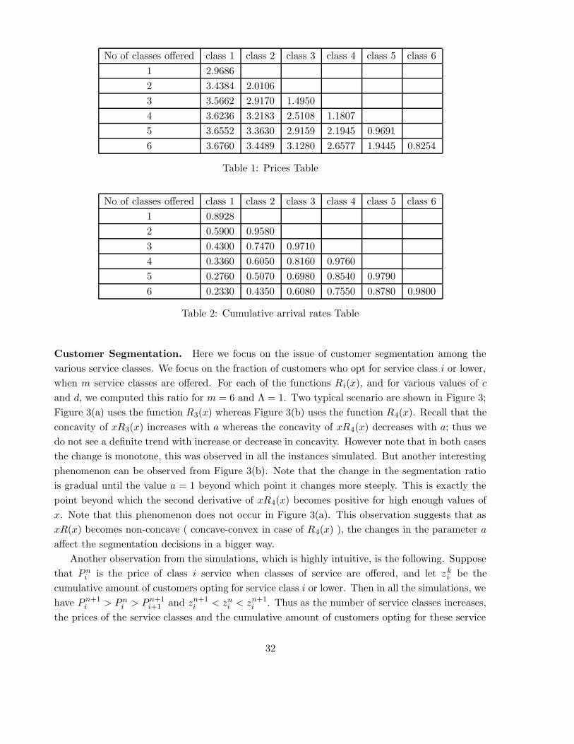
No of classes offered class 1 class 2 class 3 class 4 class 5 class 6

1 2.9686

2 3.4384 2.0106

3 3.5662 2.9170 1.4950

4 3.6236 3.2183 2.5108 1.1807

5 3.6552 3.3630 2.9159 2.1945 0.9691

6 3.6760 3.4489 3.1280 2.6577 1.9445 0.8254

Table 1: Prices Table

No of classes offered class 1 class 2 class 3 class 4 class 5 class 6

1 0.8928

2 0.5900 0.9580

3 0.4300 0.7470 0.9710

4 0.3360 0.6050 0.8160 0.9760

5 0.2760 0.5070 0.6980 0.8540 0.9790

6 0.2330 0.4350 0.6080 0.7550 0.8780 0.9800

Table 2: Cumulative arrival rates Table

Customer Segmentation. Here we focus on the issue of customer segmentation among the

various service classes. We focus on the fraction of customers who opt for service class i or lower,

when m service classes are offered. For each of the functions Ri(x), and for various values of c

and d, we computed this ratio for m = 6 and Λ = 1. Two typical scenario are shown in Figure 3;

Figure 3(a) uses the function R3(x) whereas Figure 3(b) uses the function R4(x). Recall that the

concavity of xR3(x) increases with a whereas the concavity of xR4(x) decreases with a; thus we

do not see a definite trend with increase or decrease in concavity. However note that in both cases

the change is monotone, this was observed in all the instances simulated. But another interesting

phenomenon can be observed from Figure 3(b). Note that the change in the segmentation ratio

is gradual until the value a = 1 beyond which point it changes more steeply. This is exactly the

point beyond which the second derivative of xR4(x) becomes positive for high enough values of

x. Note that this phenomenon does not occur in Figure 3(a). This observation suggests that as

xR(x) becomes non-concave ( concave-convex in case of R4(x) ), the changes in the parameter a

affect the segmentation decisions in a bigger way.

Another observation from the simulations, which is highly intuitive, is the following. Suppose

that P ni is the price of class i service when classes of service are offered, and let zk

i be the

cumulative amount of customers opting for service class i or lower. Then in all the simulations, we

have P n+1i > P n

i > P n+1i+1 and zn+1

i < zni < zn+1

i . Thus as the number of service classes increases,

the prices of the service classes and the cumulative amount of customers opting for these service

32

classes exhibit a nested property. Table 1 shows prices and Table 2 shows cumulative arrival rates

for the case R4(x), d = 0.1, c = 0; , µ = 1.35,Λ = 1.

6 Conclusions

In this paper we studied the problem of designing a profit maximizing pricing-scheduling policy

for a capacity-constrained firm with a heterogeneous customer base. The main conclusion we

draw form our analysis is that under certain conditions it might be beneficial to pool customers

of different characteristics together and treat them equally; this happens because customers self-

select their service class. The results of Theorem 6, Segmentation Algorithm, Lemma 7 and

Theorem 11 extend to the cases of M/M/1 and M/G/1 queues without preemption, and to the

M/M/s system (with a single queue) with and without preemption; the analysis in these cases

remains essentially the same. These results can also be extended to the preemptive M/G/1 case

by observing that it is enough to consider policies in which the preemption decisions are based

only on the identity of the customer types (and not on the information learned/revealed while

serving). Thus the results of our model are valid in more general settings. Also the result of

Lemma 8 can be extended to M/M/1 system without preemptions, thus providing an efficient

procedure for solving the restricted service differentiation case.

There are various avenues for extending this work. One is to extend the analysis to the setting

in which the value for obtaining service for the customers within a customer type is a random

variable and none of the customer types can be served in full. This is the same setting as in

Mendelson and Whang [28], and a similar analysis, without a priori fixing the scheduling policy

to be the the cµ rule, might work. If, in addition, it is possible to serve some of the customer types

in full, then the problem will have to be analyzed differently (as the marginal customer of some

customer type i can now have a positive surplus). The same applies for the case of heterogeneous

service requirements. These questions are the topic of ongoing research. Also given that increasing

the capacity and increasing the number of service classes are both costly, it would be interesting

to get an understanding of the situations under which one would be preferred to the other (this

might depend on the existing capacity). Finally, it would be interesting to analyze the strategies

of two service providers who face the same customer base and are free to offer as many service

levels as needed.

Acknowledgements

We are grateful to Ward Whitt for a suggestion regarding the simulations, and to Philipp Afeche

for several useful comments on an earlier draft of the paper.

33

References

[1] P.Afeche (2004),“Incentive-Compatible Reveue Management in Queuing Systems: Optimal

Strategic Idleness and other Delaying Tactics”, Working paper, Kellog school, Northwesetrn

University.

[2] P.Afeche, H.Mendelson (2004),“Pricing and Priority Auctions in Queuing Systems with a

generalized Delay Cost structure”, Management Science, 50(7), 869 - 882.

[3] K.R.Balachandran (1972),“Purchasing Priorites in Queues”, Management Science, 18(5),

319-326.

[4] A.Beja, E.Sid (1975),“Optimal Priority Assignment with Heterogeneous Waiting Costs”, Op-

erations Research, 23(1), 107 - 117.

[5] R.M.Bradford (1996),“Pricing, routing and incentive compatibility in multiserver queues”,

European Journal of Operational Reserach, 89, 226-236.

[6] R.M.Caldentey and L.M.Wein (2003),“Revenue Management of a Make-to-Stock Queue”,

Working paper, New York University, New York.

[7] E.G.Coffman Jr. and I.Mitrani (1980),“A Characterization of Waiting Time Performance

Realizable by Single-Server Queues”, Operations Research, 28(3), 810 - 821.

[8] R.W.Conway, W.L.Maxwell and L.Miller (1967), Theory of Scheduling, Add.-Wesley, Mass.

[9] D.Cox and W.Smith (1961), Queues, Methuen, London.

[10] S.Dewan and H.Mendelson (1990),“User Delay Costs and Internet Pricing for a Service Fa-

cility”, Management Science , 36(12), 1502-1517.

[11] R.J.Dolan (1978),“Mechanisms for Priority Queuing Problems”, Bell Journal of Economics,

9(2), 421-436.

[12] N.M.Edelson and K.Hilderbrand (1975),“Congestion tolls for Poisson queueing processes”,

Econometrica, 43, 81-92.

[13] A.Federgruen and H.Groenvelt (1988), “Characterization and Optimization of achievable

performance in general queuing systems”, Operations Research, 36(5), 733 - 741.

[14] S.B.Ghanem (1975),“Computing central optimization by a pricing priority policy”, IBM Sys.

Journal, 14, 272-292.

[15] A.Glazer and R.Hassin (1986),“Stable Priority Purchasing in Queues”, OR letters, 4, 285-288.

[16] D.Gupta and L.Wang (2005),“Manufacturing Capacity Revenue Management”, Working pa-

per, University of Minnesota, Minneapolis.

34

[17] A.Y.Ha (2000),“Optimal Pricing that coordinates queues with customer chosen service re-

quirements”, Management Science, 47(7), 915-930.

[18] M.Harris and R.M.Townsend (1981),“Resource allocation under assymetric information”,

Econometrica, 49, 33-64.

[19] R.Hassin (1995),“Decentralized regulation of a queue”, Management Science, 41(1), 163- 173.

[20] R.Hassin, M.Haviv (2003),“To Queue or not to Queue”, Kluwer, Boston.

[21] L.Kleinrock(1967),“Optimum Bribing for Queue Position”,Operations Research, 15, 304-318.

[22] P.J.Lederer and L.Li (1997),“Pricing, Production, Scheduling and Delivery-Time Competi-

tion”, Operations Research, 45(3), 407-420.

[23] F.T.Lui (1985),“An Equilibrium Queuing Model of Bribery”, J. Oof. Pol. Econ., 93, 760-781.

[24] C.Maglaras (2005),“Revenue management for a multi-class single-server queue”, working pa-

per, Graduate School of Business, Columbia University.

[25] C.Maglaras, A.Zeevi (2005),“Pricing and Design of Differentiated Services: Approximate

Analysis and Structural Insights”, Operations Research, 53(2), 242 - 262.

[26] M.Marchand (1974),“Priority Pricing”, Management Science, 20(7), 1131 - 1140.

[27] H.Mendelson(1985),“Pricing Computer Services: Queuing Effects”, ACM, 28, 312-321.

[28] H.Mendelson and S.Whang (1990),“Optimal Incentive-Compatible Priority pricing for the

M/M/1 Queue”, Operations Research, 38(5), 870-883.

[29] R.B.Myerson (1981),“Optimal Auction Design”, Math. of OR, 6(1), 58 - 73.

[30] P.Naor (1969), “On the Regulation of queue size by Levying tolls”, Econometrica, 37(1),

15-24.

[31] E.R.Petersen and S.Rao (1993),“A Dynamic Programming Model for Assigning Customers

to Priority Service classes”, School of Business Working Paper No. 93-24, Queen’s University,

Kingston, Canada.

[32] E.Plambeck (2004),“Optimal Leadtime Differentiation via Diffusion Approximations”, Op-

erations Research, 52(2), 213 - 228.

[33] A.Printezis, A.Burnetas (2004),“Pricing in a Single Queue with Two Customer Classes With

and Without Price Discrimination”, Working paper, Weatherhead School of Management,

Case Western reserve University.

35

[34] S.Rao and E.R.Petersen (1998),“Optimal Pricing of Priority Services”, Operations Research,

46(1), 46-56.

[35] J.Shanthikumar and D.Yao (1992), “Multiclass Queuing Systems: Polymatroidal Structure

and Optimal Scheduling Control”, Operations Research, 50(1), 197 - 216.

[36] S. Stidham Jr (2002),“Analysis, design and control of Queuing systems”, Operations Re-

search, 50 (1), 197-216.

[37] J.A.Van Mieghem (2000),“Price and Service Discrimination in Queuing Systems: Incentive

Compatibility of Gcµ Scheduling”, Management Science, 46(9), 1249-1267.

36