Copyright ©2015 byTheAmericanRadio RelayLeague, Inc.

Copyrightsecuredunder thePan-AmericanConvention

All rightsreserved.No part of

this workmay bereproducedin any formexcept bywrittenpermissionof thepublisher.All rights oftranslationarereserved.

Printed inthe USA

Quedan

reservadostodos losderechos

ISBN: 978-1-62595-023-9

First Edition

We strive to produce books withouterrors. Sometimes mistakes do occur,however. When we become aware ofproblems in our books (other thanobvious typographical errors), wepost corrections on the ARRL

website. If you think you have foundan error, please checkwww.arrl.org/notes for corrections.If you don’t find a correction there,please let us know by sending e-mailto pubsfdbk@arrl.org.

eBooks created bywww.ebookconversion.com

Contents

ForewordPrefaceAcknowledgementsAbout the AuthorDedication

1 Why Get an Oscillscope?2 A Little History3 Every Scope Has These Elements4 Probes and Accessories5 Scope Sections in Detail6 Input Modes7 Let’s Put a Scope to Work8 If You Are Going to Buy One —

SpecificationsAppendix 1Software Oscilloscopes — Capableand Free!Appendix 2QST Product Review: TektronixTBS1042 and Rigol DS1052EOscilloscopesAppendix 3QST Product Review: OsciumiMOS-204 Portable Oscilloscope

Foreword

A popular activity among amateurs isbuilding, modifying, restoring orrepairing equipment. During theircareers, amateurs assemble a homeworkshop appropriate for their interests,usually starting with a few basic tools, agood soldering iron and perhaps amultimeter. From there, you might add apower/SWR meter or an antennaanalyzer.

When it comes to working inside apiece of equipment, one of the mostuseful tools is the oscilloscope.“Scopes” have been around for decades,

helping countless amateurs “see” thesignals inside their equipment. Is mySSB transmitter properly adjusted? Whatdoes my CW waveform look like? Isthere ripple on my power supply? Oncean expensive tool for only the mosttechnically savvy amateur, today wehave access to a variety of analog,digital or hybrid scopes at pricessuitable for a home workshop.

In this book, Paul Danzer, N1II,conveys a wealth of information aboutthese useful tools. Starting with anoverview and short history lesson, Paulgoes on to discuss oscilloscopefunctional blocks, probes, controls andinput modes and then describes practical

applications. He concludes with achapter to help you understand scopespecifications and features so that youcan find one that will best suit yourneeds.

We hope you’ll find this book auseful addition to your library.

David Sumner, K1ZZChief Executive OfficerNewington, ConnecticutFebruary 2015

Preface

As every teacher knows,occasionally you are rewarded by a fewstudents who want to know a bit more ona topic that your lecture or the textbookcovered. This is especialy true when youmention to a class, as I did, that theoscilloscope is a very valuable tool inelectronics — ham radio or otherwise— simply because it lets you “see” whatis going on!

Years ago the same oscilloscopeblock diagram and the same explanationwere found in most books. Today, withthe introduction of personal computers,

digital technology and the ability toproduce oscilloscopes with morecapability at a lower cost, the entirefield has changed.

In particular, there still are quite afew totally analog oscilloscopesavailable, but there are also many newconfigurations. Some are totally self-contained digital instruments, some are adigital/analog hybrid, some require apersonal computer to act as theprocessor and display, and others usesmartphones phones and tablets as theirhost.

Most books and online descriptionsreflect either the old analogconfiguration or advanced theory beyond

what many students and radio amateurscan profitably use. This book waswritten to discuss oscilloscopes in amiddle ground — past the simple analogscope, but less than a graduate leveltreatise in data processing and signalcomputations.

Today’s technologies have madevery capable oscilloscopes available toradio amateurs for many uses in the hamshack. There are two reasons for thisavailability. First, the new digitalscopes have displaced the older, veryexpensive scopes in businesses andindustrial labs. As a result, scopes withcapabilities most of us could only dreamof years ago are often available used at a

price of one tenth or less of theiroriginal price. Second, the new digitalscopes are, due to the use of digitalprocessing, not dependent on precisionanalog circuits and therefore lessexpensive than their predecessors.

The result is that the ability to “seewhat is going on” in our equipment ismuch more available and much morecommon in the ham shack.

73, Paul Danzer, N1II(past call signs: KN2DGR, K2DGR,

W1DQJ)

Acknowledgements

Many thanks to the followingindividuals, companies andorganizations who were very generouswith their time and help:

Jim Brannigan, WB2TPSDave Cisco, W4AXLSam Dick, NV1PSeth Golitzer, W1SHGDon Hudson, KA1TZRChuck Penson, WA7ZZERon Pollack, K2RPRich Roznoy, K1OFJoe Veras, K9OCO

Tim Walker, W1GIGMark Wilson, K1RO

Alex Wong at Digilent Inc.Bryan Lee at OSCIUM, Dechnia,

LLCChuck at www.myvintagetv.comTekwiki, the community of Tektronix

oscilloscope enthusiasts,www.w140.com/tekwiki

About the Author

Paul Danzer, N1II, started hisAmateur Radio career as a teenager,which led to Bachelor’s and Master’sDegrees in Electrical Engineering. Hisengineering career spanned more than 30years, and he was awarded 11 patentswhile specializing in digital circuits,digital systems, and radar systems. As aresult he had a great deal of hands-onexperience with the subject of this book,oscilloscopes.

After retiring from engineering, hespent three years as a Technical Editorat ARRL Headquarters in Newington,

Connecticut. There, he authored onebook, co-authored a second and editedt h e ARRL Handbook and the ARRLOperating Manual as well as severalother publications.

Paul then embarked on a new careeras a Professor of Computer Science at alocal community college, teachingelectronics, personal computerhardware, data communications andother PC related subjects. After 11 yearsas a full time professor he is now anAdjunct Professor and spends the rest ofhis time writing on Amateur Radiosubjects.

He has written more than 250magazine articles for Amateur Radio

publications and computer publications.His ARRL appointments include TA(Technical Advisor) and TS (TechnicalSpecialist). In 2004, he was awarded theBill Orr, W6SAI Technical WritingAward by the ARRL Board of Directors.

Dedication

To my wife Flo, who has patientlytolerated strange noises, strange wires,and all sorts of strange things attached tothe roof of our home.

Chapter 1

Why Get anOscilloscope?

Didn’t you ever say, “I wish I couldsee what was going on?”

That is the question hams have beenasking since the earliest days of hamradio. By nature, not only do hams liketo experiment, but they also want to getthe most out of their equipment. Can youimagine a cook, busy preparing a meal,

who cannot smell or taste the food? Thatis exactly the situation many hams findthemselves in when they are testing,repairing or just using their gear.

Every piece of test equipment has itsplace, and an on-the-air test can be veryrevealing. But to really understand whatis going on — just like a cook in thekitchen has to taste dishes with his or hertongue — you have to literally see withyour eyes to really understand a circuitor equipment.

Some years ago this ability to seewas beyond the budget of most hams,except for a few who built their ownoscilloscopes. Professional-gradescopes cost $1500 to $3500 and

required periodic calibration with testequipment that was more expensive thanthe scopes themselves. Industrial surplusequipment or lesser grade scopes,including kits, were not cheap. Youwould have to write a check for $300 to$600 and you were never sure just howaccurate your measurements were.

In addition to requiring periodiccalibration, this generation of scopesused vacuum tubes that that ran hot,increased the amount of and frequency ofcalibration, and increasingly caused theoscilloscopes to deteriorate inperformance.

Since those days there have been twomajor changes: Solid state devices

(transistors, diodes, integrated circuits)have replaced vacuum tube circuitry anddigital techniques have replaced driftinganalog circuits. Perhaps the result ofthese changes can best be seen bycomparing the pictures in this chapter.

What Do Oscilloscopes Oldand New Look Like?

The older generation high-qualityanalog scope, such as the Tektronix unitshown in Figure 1.1, represents a typeof scope that was a laboratory standardthrough many model number variations.Generally these scopes weighed morethan 60 pounds and were mounted on a

cart because they were not carriedeasily. Power input was about 700 W,so a small lab space could get quite hot.You can see the tube lineup of this beastin Figure 1.2.

Technician quality scopes such asmight be found in a well-equipped (andwell-funded) home lab or on the benchof a TV repair shop in the past typicallylooked like the one in Figure 1.3 — anEICO 460. For the most part thesescopes did not do precisionmeasurement as the Tektronix did, butstill answered the question “What isgoing on?” In the case of the TV repairshop or the ham workshop, it answeredthe question “Is the signal there?”

By comparison, many of today’sscopes look like the one Figure 1.4. Itmeasures roughly 2 × 8 × 7 inches,weighs 1.5 pounds, and plugs into acomputer USB port for power. Exceptfor the input circuit, the rest of the scopeis digital. There is no screen or display;the scope feeds a desktop or laptopcomputer. Calibration is usually built in,and the digital circuits are often givenadditional tasks such as acting as asignal generator or a spectrum analyzer.The most amazing part is the cost —anywhere from less than $100 to perhaps$350 for fairly accurate measurements.

There is one other major change fromthe older analog oscilloscopes to the

newer digital scopes. Often the scope isused to find out “What Happened?” Thismeans looking for something thathappens briefly, not continuously. Witholder analog scopes, their native modeof operation was continuousmeasurement. You would have to watchthe display carefully to catch transient or“occasionally here, usually not” things.To be able to capture and hold transientmeasurements, you would need to ownan even more expensive storage scope.Storage scopes could capture anddisplay a transient waveform on aspecial phosphor screen that had long-term holding capability.

The native mode of the new digitalscope is storage. Input waveforms aresent to a digital memory. Unlesscommanded to erase or replace the olddata with new data, they automaticallystore their inputs to the limit of the sizeof their memory.

What Can You Do WithYour Scope?

Later on, in Chapter 7, we will take alook at many of the common uses of anoscilloscope in the ham shack. But fornow, let’s just get an idea of what thesedevices can do for you.

If you opened a copy of the ARRL

Handbook of 30 or 40 years ago, thefirst application for scopes would be tolook at your transmitted AM signal. Thiswas a very good way to tell if you hadyour transmitter adjusted correctly or ifyou were over modulating, thusspattering all over the band in additionto sounding terrible. In Chapter 7 wewill take a look at this application, butfor now look at the block diagram inFigure 1.5. Here is a problem yourscope could help you with, and at leasttell you what is going on.

Suddenly your friends on the repeatercomplain that your 2 meter transceiver athome has a terrible hum. Because youare conscious of public service and

emergency communications, you run thisradio from a 12 V storage battery with atrickle charger. You can think of threepossibilities.

First, is the hum coming from thetrickle charger/battery combination? Outcomes your scope, you connect it atpoint A, from the +12 V line to ground,and this possibility is quickly confirmedor eliminated. Is the 12 V line a pure dcsignal or is there an ac component to thewaveform?

Next, is the problem in the audiochain? Perhaps it is a bad microphonecord or something in the microphoneamplifier. Connect the scope to point Band now you can tell if the hum is

coming from this set of circuits.Finally, perhaps the

synthesizer/phase-locked loop is havinga problem. Your friends tell you that thehum sounds like 60 Hz, so look atvarious places around the synthesizer.You don’t have to know what waveformyou are looking at, nor do you need tosee each individual signal in detail.Look for an envelope that has repetitivechanges corresponding to theapproximate period of a 60 Hzwaveform — perhaps at point C.

Is this approach guaranteed to helpyou solve the problem? Of course not,but you can actually see what is going onat these key points in the circuit, so you

stand a better chance of finding a cure.Maybe you will be lucky and it is just abad ground on your microphone cord.

Figure 1.6 shows another verycommon use for oscilloscopes. With afew more components you can testdiodes, capacitors, resistors, andtransistors. In Chapter 7 we will discussthis use and others in more detail. InFigure 1.6, the component being tested isa standard diode — perhaps a powerrectifier. By picking the correctcomponents and oscilloscope settings, aV-I (voltage vs current) curve appearson the scope display. If the diode isokay, the V-I curve will look like theleft-hand drawing, if shorted, the centerdrawing, and if open the right-handdrawing.

An oscilloscope in your shack is

more than just a handy test instrument; itlets you both solve problems and testnew ideas. Chapter 2 will explain a bitof where oscilloscopes came from andhow the inexpensive but very capableunits we have today were developed forthe older — occasionally very mucholder — technology.

Chapter 2

A Little History

We’ve come a long way. In order tounderstand why oscilloscopes have thedesigns and capabilities they have today,it is helpful to see where they came fromand how they developed. In the nextchapter you will see that everyoscilloscope — whether it is builtentirely in hardware, partly in hardwareand partly in software or even totally insoftware — has the same four elements

or sections. One reason for thiscommonality is history.

The changes in oscilloscopes fromthe late 1800s to the present result froma two-edged sword. As the technologychanged, the requirements foroscilloscopes changed and thecomponents that could be used in thedesign of oscilloscopes changed — bothfactors changing in parallel. This chaptersummarizes how the oscilloscopes wehave available to us in our ham shacksand workbenches developed andchanged over the years. A full historywould occupy more than this entirebook, but a brief glance serves toexplain where we are and how we got

here. In particular, this chapter explainshow hams have gone from rarely owningand using oscilloscopes to being able toafford and use today’s commonlyavailable low-cost scopes if they sodesire.

Early InstrumentsThe need to “see” a voltage, current

or other physical item dates back to theearliest electrical design. It would comeas no surprise that the limit to “seeing”was how fast the measuring instrumentcould respond, how fast you could seethe response, and perhaps mostimportant — how fast you could write it

down.Very quick mechanical “scribers” —

what today we would call plotters —were invented. As Figure 2.1 shows, atypical early model consisted of amodified meter such as a standardD’Arsonval voltmeter with an extendedpointer. On the end of the pointer waseither a pen with a roll of paper or ametal pin or scribe that left animpression on a treated paper. The meteris mounted over the paper. The motionof the pen provides the X-axis(amplitude of the voltage beingmeasured), and the paper motionprovides the Y-axis (time scale). In thiscrude implementation, the amplitude

scale is not linear, and various clevermechanical ways were invented to makeit linear.

Since the meter pointer does notmove very quickly, other measurementtechniques were found. Some usedmirrors and light on photographicsensitive paper to allow the instrumentto be more responsive and to plot higherfrequency signals.

The Cathode Ray Tube(CRT) Changed Everything

It is always a problem to state withabsolute certainty who was the firstperson to do something or the firstperson to invent something. As anexample, the Smithsonian in WashingtonDC has an entire exhibit paying tribute tothe Wright Brothers for making the firstflight. But in Connecticut there is arecord of an earlier flight, described in anewspaper of the time. The French havetheir own candidate for first flight, as dothe Germans and others.

Knowing that, let’s start with KarlBraun, who is credited with making acold-cathode ray tube in 1897, and is

recorded as using it to explore thewaveform of an alternating currentvoltage. Thus, in effect, he made andused an oscilloscope. However, thiswas before the first recorded vacuumtube amplifier demonstrated by Sir JohnAmbrose Fleming in 1912. Undoubtedlythere are other candidates to claim thatthey should have the “first to do” title ofthese developments, but these things doform the basis of today’s oscilloscopes.

Fast forwarding now to pre-WorldWar II, Figure 2.2 shows a state of-the-

art oscilloscope for hams in 1937. Thisdevice, the National Radio Companymodel CRM, would be recognized as afunctional piece of test equipment thatcould be used by most hams today —although of limited bandwidth andaccuracy. The price, as advertised inQST in the late 1930s, was — ready forthis one? — $11.10 plus an additional$5.81 for the cathode ray tube.

By 1947 hams had graduated to theNational CRU oscilloscope, with a 2-inch tube (Figure 2.3). From the pictureit seems to have a sweep trigger control.At the same time, World War II surplusgear was very common, so many hamswere building their own version of theNational scope. Then the HeathCompany, which started out in lifeselling airplane kits, came out with itsfirst electronic kit — the O-1oscilloscope. Key to this kit was, as youmight guess, the large stock of war-surplus cathode ray tubes available onthe market. Figure 2.4 is an earlyHeathkit scope kit selling for $39.50.

About the same time a new homedevice — television — was capturingimaginations. Using tubes and highvoltages, these TV sets required frequentrepair, so many TV repair shops sprang

up . Figure 2.5 is an example of thetypical oscilloscope found in many TVshops, a Dumont 274. RCA, which at thetime was a TV manufacturer, acommunications company and aneducational institute, jumped in with itsstudent-oriented scope in Figure 2.6.Now hams had three sources ofoscilloscopes for the shack andworkbench — kits such as the Heath andEico, moderately priced commercialunits such as Dumont and RCA, and, ofcourse, home built.

My Heathkit OscilloscopeClone

By Tim Walker, W1GIGIn the early 1960s, when I had a

young family and was struggling tofinish my new house in Utica, NewYork, I needed a scope to servicemy hi-fi gear. I had previously builtone from the ARRL Handbook thatused a small diameter 913 tube forthe display, but a 1-inch scope hasits limitations. Searching through thesurplus stores in the area produceda 3AP1 tube (a 3-inch CRT) and ascope power transformer. Of courseI had the current Heath catalog andin it found the plans for a very nice3-inch scope. Remember, Heathused to include the circuit diagram

for many products in their catalogs.Using mostly parts from my junk boxI put the scope together and used ithappily.

A couple of years later, afterbeing transferred to New York City,I found that my new office was in themiddle of Radio Row, at the time thesurplus electronics center of theuniverse. You can bet that I spentmany a lunch hour checking out allthe stores. One day I came upon a3ACP1 smiling at me from thewindow of one of my favorite stores.The flat face of the tube promisedme a much better scope. For about$5, I got the tube, the mu metalshield and the special 14-pin socket.Now how to use it?

I found that the Heath design hadbeen updated to use the 3BP1 and

miniature tubes. It was now calledthe IO-21. The only problem wasthat the 3ACP1 had an acceleratinganode that requires 4000 V abovethe cathode, so I rebuilt the highvoltage power supply for my new3ACP1.

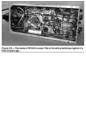
I have been using this scope forabout 50 years now. As you can seefrom the photographs it looks tired,the parts are old and look large ascompared to today’s parts — but itstill works and works well!

Advances in IndustryIn the 1960s, 70s and 80s,

commercial electronics labs outgrew theDumonts in favor of precision laboratoryscopes. Tektronix was perhaps the mostcommon name seen in commercialdevelopment and military contractorlabs, followed by Hewlett-Packard.They had several things in common:

They were expensive — severalthousand dollars to more than $10,000.

They were heavy — often theywere mounted on a cart

They required a great deal ofmaintenance, including tube replacementand calibration.

They often required air conditionedrooms because they radiated a lot of heatand did not fare well in high humidity.

Typical of this generation is theapproximately 70-pound Tektronix 535shown in Figure 2.7. At the lower left isan exchangeable front end that allowedthe scope to be used for variouspurposes, but this room-warmerdissipated around a half-kilowatt! Assucceeding generations of scopes werereplaced with newer and more capableunits, these vacuum tube based unitsoften were sold for a few hundreddollars — which meant that they endedtheir lives in a ham workshop.

Of course, as you might expect, theappearance of the transistor andintegrated circuit changed thingscompletely. By comparison the solid-state Tektronix 2215A in Figure 2.8weighs around 15 pounds, dissipates 40W and is typical of this later generationof scopes. As happened with thepreceding tube-based scopes, newer andnewer units replaced the older ones inthe industrial labs. Once again, for a fewhundred dollars (and often less) thenewer solid-state units replaced theolder ones in ham workshops.

Companies such as BK Precision(Figure 2.9) jumped in to supply repairshops and more well-funded hams. Andof course Heath remained a hamworkshop favorite with models such asthe 4554 (Figure 2.10) Suddenly hamsno longer need to shop for obsolete tube-based scopes!

Today’s ChoicesToday — do you want a new scope

for $150-$350? Take a look at Figure2.11. This instrument is dual channel,includes self-calibration, is solid state,includes every mode that the olderscopes had and more. But where is the

display screen?

The answer is, it is attached to yourdesktop PC or laptop and uses thecomputer’s monitor. Only the analogfront end, A/D converters and somedigital control circuits are in the small

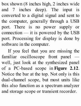
box shown (8 inches high, 2 inches wideand 7 inches deep). The input isconverted to a digital signal and sent tothe computer, generally through a USBport. There is no power supply orconnection — it is powered by the USBport. Processing for display is done bysoftware in the computer.

If you feel that you are missing thefamiliar oscilloscope front panel —well, just look at the synthesized panelof a PC-based scope in Figure 2.12.Notice the bar at the top. Not only is thisdual-channel scope, but most units likethis also function as a spectrum analyzerand storage scope or transient recorder.

If you still like the idea of a self-contained oscilloscope with built-indisplay screen, low-cost digital storageoscilloscopes such as the one shown inFigure 2.13 are available from a numberof manufacturers. Costing as little as

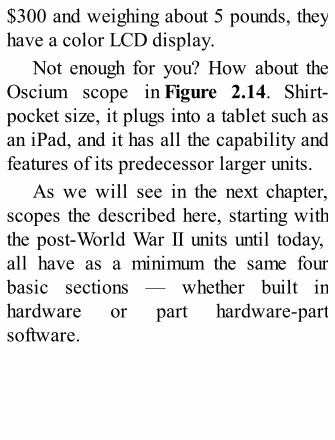
$300 and weighing about 5 pounds, theyhave a color LCD display.

Not enough for you? How about theOscium scope in Figure 2.14. Shirt-pocket size, it plugs into a tablet such asan iPad, and it has all the capability andfeatures of its predecessor larger units.

As we will see in the next chapter,scopes the described here, starting withthe post-World War II units until today,all have as a minimum the same fourbasic sections — whether built inhardware or part hardware-partsoftware.

Chapter 3

Every Scope HasThese Elements

Every oscilloscope contains the fourfunctional parts shown in Figure 3.1.Notice the word functional. Early in thehistory of oscilloscopes there weregenerally four actual circuit sections, butnot today. When microprocessors, fastanalog-to-digital (A/D) converters,personal computers and flat panel

displays made their appearance,oscilloscopes reflected these newtechnologies.

Today’s scopes are part hardware,part software, sometimes part personalcomputer (or laptop, netbook, tablet, andso on). Sometimes they are evensoftware alone.

You might also notice that a fifthfunctional area, a power supply, is notincluded in the figure. The reason issimple — many modern scopes do nothave an internal power supply. They use

power taken from a USB port or otherconnection to a computing host.

This chapter briefly describes eachof the four functional areas. Later, inChapter 6, you will find more details onthese sections and their capabilities.

Vertical Circuits Handle theInput Signals

Other than the power supply, thevertical circuit or vertical channel isthe only part of an oscilloscope that mustbe designed, at least in part, as an analogcircuit. The object of the vertical circuitis to put the waveform on the screenwith minimum distortion. It must also be

able to limit the voltage of the inputsignal — perhaps attenuate it, inconjunction with a test probe, or amplifyit — so that it falls within the limits ofthe circuits that follow.

Figure 3.2 is a simplified blockdiagram of an input stage. The firstswitch allows you to select DC and seethe absolute level of a signal. The

second position is AC — in general acapacitor blocks the dc voltage and onlythe ac component is seen. Quite oftenthere is a third selection — GROUND.This is used to position the trace,without a signal, anywhere you wish onthe screen.

Most scopes have an overlay on thescreen, called a graticule. Analogscopes typically have the graticule as aphysical plastic overlay, while modern

digital scopes often use an electronicpattern on the screen. As seen in Figure3.3, it is customary to have the graticulecalibrated in centimeters, and as a resultthe input voltage scale is usually statedi n volts per centimeter (V/cm). Thehorizontal time scale is usuallydescribed in seconds, milliseconds,microseconds or other time units percentimeter — such as 3 ms/cm or 3milliseconds per centimeter.

An expanded block diagram is shown

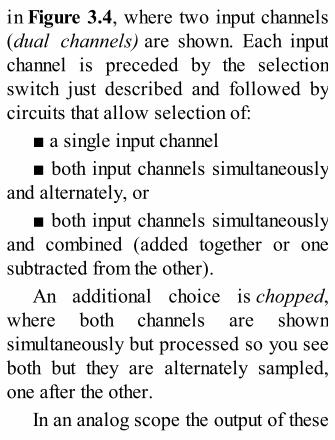
in Figure 3.4, where two input channels(dual channels) are shown. Each inputchannel is preceded by the selectionswitch just described and followed bycircuits that allow selection of:

a single input channel both input channels simultaneously

and alternately, or both input channels simultaneously

and combined (added together or onesubtracted from the other).

An additional choice is chopped,where both channels are shownsimultaneously but processed so you seeboth but they are alternately sampled,one after the other.

In an analog scope the output of these

stages goes to additional amplifier. Inmany modern scopes, the first stageoutput goes to A/D converters (Figure3.5) and the channel selection is done inprocessing past the A/D converters.

The Horizontal SectionSweeps the Trace Across theScreen

Since an oscilloscope usually showsa quantity — say a voltage — as itvaries with time, the horizontal axisrepresents time. The start of time, orwhat is generally called t = 0, is on theleft side of the screen. How fast the tracemoves across the screen is the sweep

rate. This can vary from seconds percentimeter (s/cm) to nanoseconds percentimeter (ns/cm). Lower sweep ratesare used for voltages that vary slowly.

As an example, suppose you wantedto take a close look at a 60 Hz sinewave. The time for one such wave, orthe period, is calculated as 1/frequencyor 1/60 of a second — or approximately16.66 ms (milliseconds). Mostoscilloscopes have a graticulecalibrated as 10 centimeters (cm) wide.A sweep rate of 2 ms/cm would have thetrace cross the entire 10 cm wide screenin 20 ms, so a bit more than one cycle(16.66 ms) of the 60 Hz waveformwould be seen.

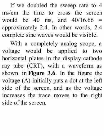
If we doubled the sweep rate to 4ms/cm the time to cross the screenwould be 40 ms, and 40/16.66 =approximately 2.4. In other words, 2.4complete sine waves would be visible.

With a completely analog scope, avoltage would be applied to twohorizontal plates in the display cathoderay tube (CRT), with a waveform asshown in Figure 3.6. In the figure thevoltage (A) initially puts a dot at the leftside of the screen, and as the voltageincreases the trace moves to the rightside of the screen.

Today, of course, most scopes do notuse CRTs and the output goes to adigitally-generated display — usually aflat screen LCD of some sort. In thiscase, the analog voltage of Figure 3.6would be replaced by a digital count. Acount of zero would place the dot at theleft edge, and as the count increases thetrace would move to the right. Sweepspeed would be controlled digitally.

You can look at the horizontal positionas the count in a digital counter — thefaster the input clock to the counter, thefaster the trace goes across. In otherwords, the faster the input clock, smallerthe time per cm.

Some oscilloscopes have anadditional mode, where the sweepcircuit is disabled and one channel, saychannel A, is connected as usual to thevertical axis and the second channel,

channel B, is connected to the horizontalaxis. This permits an on-screen plot ofone signal against another. Where thefrequencies of two signals are related,say one is a sine wave at 1000 Hz andthe other a sine wave at 3000 Hz, thepattern will tell you the frequencyrelationship by counting the lobes on thescreen. This display is called aLissajous pattern and the one shown inFigure 3.7 has a 3:1 relationship.

At this point you can see that aoscilloscope today could be totallyanalog, with precision analog circuitsand a CRT display. Or, a scope can betotally digital, converting the analoginput immediately to digital and

processing it and the sweep in digitalcircuitry. Many scopes are in fact acombination of the two.

The Sync Circuit Triggersthe Sweep

All scopes, digital or analog, musthave a way to make the displayedwaveform seem to stand still on thescreen. This is the function of thesynchronization or sync circuits. If welet the sweep circuit run free — there isno relationship to the input waveform —the waveform in Figure 3.8 is the result.Each successive input waveform startsat a different point, and after a number of

input waveforms the entire screen fills.However, if we trigger the sweep sothat each sweep starts as the inputwaveform equals a set voltage — as inFigure 3.9 — then a single waveform isseen. Actually it is many waveforms, butperfectly superimposed on each other.Figure 3.9 shows two trigger points. Fortrigger point A, +1 V is selected with apositive slope. Point B shows where thetrigger point would be if +1 V isselected with a negative slope.

Individual scopes have sets of triggerselection features. Generally there is avoltage level selection that determineswhere on the input waveform the sweepshould start. Often there is a slope

selection — whether the selectedvoltage trigger point should be on arising waveform or a falling waveform.Additional choices include pickingeither channel A or channel B for synctrigger, ac coupling or dc coupling to thesync circuit and often a line or 60 Hzsync input on older scopes.

Should you decide to buy an olderscope, don’t be surprised if the syncselection also has positions labeledHORIZONTAL and VERTICAL. These werepositions used to service analog TV setsbefore the switch over to digital TV.

While the sweep usually is triggered— starts — immediately as the selectedtrigger point occurs, more complex

scopes (often more expensive scopes)often have a delay feature. The triggerselection picks the start point, but theactual sweep does not start until a laterselected time. This feature is known asthe sweep delay. In Chapter 6 we willdiscuss one of these delay features thathas some interesting ham radioapplications.

Display TypesCurrently there are three popular

oscilloscope displays: a cathode raytube (CRT), a flat panel LCD or TFTdisplay such as used with most personalcomputers, and … none. The first twoare physical, and integrated into theoscilloscope cabinet or enclosure. Thelast represents modern scopes thatconsist of a processing front end pluggedinto a PC, tablet or even a smartphone.

Classic Cathode Ray TubeThe cathode ray tube, or CRT, was

the earliest oscilloscope displaycomponent. For a screen size of five orso inches across, the scope designer had

to use a package that was fairly deep (12inches or more) and allowed a greatdeal of heat to be radiated. Mostimportant of all, the CRT required apower supply of perhaps severalthousand volts.

The back end of a CRT resembles astandard vacuum tube (Figure 3.10) witha filament to heat the cathode. Electronsradiating from the cathode pass through agrid and are then pulled forward towardthe screen by a combination of a positivevoltage on a hollow anode and a highpositive voltage applied to conductivelayers on the sides toward the front ofthe tube.

The spot where the electron steam

hits the phosphor-coated front screenilluminated a dot. The position of the dotis controlled by four deflection plates.Figure 3.11 illustrates the plates,showing an illuminated spot toward theupper left corner. The electron stream ispulled up by having the voltage on plateA positive with respect to plate B. In thesame way the spot is on the left becausethe voltage on plate C is positive withrespect to plate D. If there were novoltage difference between A and B, andno difference between C and D, the spotwould be in the middle of the screen.

Brightness is controlled by the grid,just as the grid in an ordinary vacuumtube controls the flow of electrons

toward the plate. The vertical channel isconnected to plates A and B, and thesweep circuits connect to plates C andD.

Self-Contined Flat Panel DisplayUnlike the CRT, newer scopes

incorporating flat panel displays do notrequire a deep enclosure, do not needhigh voltage and do not generate a greatdeal of heat. A good scope display, likea good TV screen, does require a devicewith reasonable resolution, a very flatface and a long life.

Typical of such a display is the oneused in the Rigol DS1052e, pictured inFigure 3.12. It has a 5.6-inch diagonal

color LCD (liquid-crystal display)screen using TFT (thin film transistor)technology. Very similar displays arenow being offered on the front panel ofAmateur Radio transceivers fromseveral manufacturers.

The scope size is driven by the frontpanel, containing the display and the

manual controls (knobs and switches).The depth, approximately 5 inches, is allthat is needed to contain the circuitry ofa very capable scope.

No Display, No Power SupplyImagine taking the scope in Figure

3.12, eliminating the front panel and justpackaging the internal circuit board —perhaps in a package 1-1/2 inches wideby a few inches high and 5 inches or sodeep. The front panel holds jacks fortwo probes and the rear panel aconnector for a USB cable to a personalcomputer. The USB port supplies powerto the scope and the signal lines in theUSB cable feed the two channel inputs,

digitized, to the personal computer.Figure 1.4 in Chapter 1 shows one suchscope.

Figure 3.13 shows an even smaller— although less capable — scope, theOscium iMSO-204. It plugs directly intoan iPad, iPhone or other Apple device.Similar models, roughly 2.5 × 3.25 ×0.75 inches, are available with USBconnections.

Some Scopes Can StoreYour Waveform

Today’s technology has brought ussome interesting capabilities, somedirectly and some indirectly. With anolder scope, if you had a waveform thatyou wanted to look at in detail, and itoccurred only once, you would have to

look very quickly. When the image seenthrough the illuminated phosphor on thescreen faded, so did your capability tolook.

Some older analog scopes hadstorage capability. The CRT had aspecial phosphor and voltage circuitrythat permitted a long persistence on thescreen. Generally, storage scopescommanded a much higher price thanconventional scopes.

With today’s scopes that digitize theincoming waveforms, storage capabilityis the normal mode. Each increment ofthe waveform is stored as a digitalnumber. During each new sweep acrossthe screen these numbers are replaced bythe new incoming waveform voltages —a new set of numbers. Want storage of a

waveform? Just inhibit the new set ofnumbers. Get one sweep, hold thenumbers and look as long as you want!

Since each point on the incomingwaveform is held as a digital number,you can get indirect benefits — mathfunctions are almost free, since they arejust digital processing. As an example,look at the triangular waveshape inFigure 3.14. Want to know the peak-to-peak voltage? Find the highest number(point A in the drawing) and the lowestnumber (point B in the drawing), take thetwo digital numbers, subtract, and youhave the peak-to-peak value.

Want the period? Pick a point on thewaveform (here point C, which is a zero

crossing with a positive slope) and acorresponding point D. Measure the timebetween the two and you have theperiod. Calculate average? CalculateRMS? The scope has the data in digitalform; the calculations are fairly simplesince you are using a digital processor.Of course you don’t pick the points anddo the math; the software does it for you.

Where waveform storage used to bean expensive option, it is now the normwith a number of indirect features —calculations and numericalmeasurements — readily available.

Chapter 4

Probes andAccessories

Suppose it is a beautiful day outside.You look through the window — the sunis shining, the grass is green, the air isclear and you can see some small birdspecking around on the grass. Nowchange things a bit. Leave the outside asit was, but make the window dirty. It hasbeen splashed by mud, coated by greasy

fumes and sticky dust, and it casts anuneven gray over the scene. Now youlook out and suddenly the beautiful daylooks dreary and unappealing. What yousee is not what is there.

The same situation occurs with anoscilloscope. The probe or probesconnect the signal you want to see withthe oscilloscope input circuits. Theprobe can have a major effect on whatyou see, yet many people take it forgranted.

Do You Really Need aProbe?

In an ideal world, you could find a

probe that you could ignore. Such aprobe would be easy to use — justconnect it to your circuit. It would notdistort the signal in any way, it wouldlook to the circuit as though nothingwere connected (does not load down thecircuit), and random noise pulses fromother circuit elements would be rejectedif there were any!

Of course this is not an ideal world,and a perfect probe does not exist. Tosee what does exist, first we have toremember that when you are looking at asignal at one frequency it hascomponents — we will see shortly whatis meant by components — at manyfrequencies. Remember: if you are

looking at a 7 MHz square or sawtoothwaveform, this is the same 7 MHz as theRF coming out of your transmitter whenyou are operating on 40 meters. Youwould not expect to run a 40 metersignal down a single 12 or 18 inch longpiece of wire without having some sortof problem. At a minimum you woulduse a piece of coaxial cable or specialshielded wire — and this is where theproblem begins.

There are a few very limited caseswhere a short — say 6 inch long —piece of wire could be used, such as thefour logic signal inputs on the OsciumiPad oscilloscope described in Chapter3. This is a very special case where the

signals are limited to relatively lowfrequencies (that scope has a 5 MHzbandwidth). Actual signal shape is lessimportant and logic signal position is theimportant item.

What Does a Probe LookLike from the Signal’s Pointof View?

Let’s suppose you have a scope witha 100 MHz bandwidth and the probeconsists of a piece of coax, with thecenter of the coax connected to the signalyou wish to see. Figure 4.1 is a modelof a piece of coax. Notice that it hasinductance, resistance, and capacitance

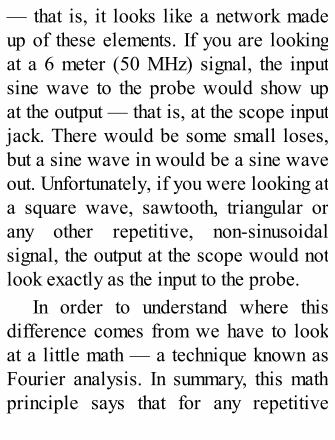
— that is, it looks like a network madeup of these elements. If you are lookingat a 6 meter (50 MHz) signal, the inputsine wave to the probe would show upat the output — that is, at the scope inputjack. There would be some small loses,but a sine wave in would be a sine waveout. Unfortunately, if you were looking ata square wave, sawtooth, triangular orany other repetitive, non-sinusoidalsignal, the output at the scope would notlook exactly as the input to the probe.

In order to understand where thisdifference comes from we have to lookat a little math — a technique known asFourier analysis. In summary, this mathprinciple says that for any repetitive

waveform (yes it holds for allwaveforms) the waveshape is actuallycomposed of a set of overlapping sinew aves . Figure 4.2 shows how thishappens, using a symmetrical squarewave for illustration.

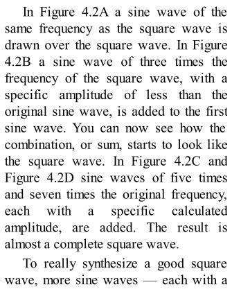
In Figure 4.2A a sine wave of thesame frequency as the square wave isdrawn over the square wave. In Figure4.2B a sine wave of three times thefrequency of the square wave, with aspecific amplitude of less than theoriginal sine wave, is added to the firstsine wave. You can now see how thecombination, or sum, starts to look likethe square wave. In Figure 4.2C andFigure 4.2D sine waves of five timesand seven times the original frequency,each with a specific calculatedamplitude, are added. The result isalmost a complete square wave.

To really synthesize a good squarewave, more sine waves — each with a

different amplitude at odd multiples ofthe base frequency — would be addeduntil the result was a perfect squarewave. Now let’s look at a 7 MHz squarewave. It would consist of sine waves at7, 21, 35, 49 (and so on) MHz — sinewaves at odd multiples of 7 MHz, eachwith its own amplitude.

Looking back at Figure 4.1, theconnecting coax has inductance,capacitance, and even some resistance.

Each of these input waves would have adifferent attenuation and phase shift. Sothe output resulting from thesimultaneous input sine waves at 7, 21,35 MHz, and so on would no longer addup to the nice square wave we startedwith at the input. For this reason anoscilloscope probe gets a bit moreinvolved. Figure 4.3 shows a standard,inexpensive scope probe. The solutionto the problem of unequal proberesponse to varying frequency is calledcompensation. In the photo notice thescrewdriver slot, located just below theground wire connection. This is thecompensation adjustment.

Probe CompensationEach probe manufacturer includes a

compensation network to equalize theprobe response to various frequencies.A very minimal network is shown inFigure 4.4. R1 and C1 — where C1 isvariable — provide the compensationfor the combination that consists of thecoax or shielded wire and the scopeinput circuit. The scope input acts as thetermination of this combination, withresistor values in the megohm region andcapacitance of perhaps 5 to 25 pF.

A second resistor and perhaps othercomponents would be added to theprobe for the ×10 attenuation selection.This is usually controlled by a slideswitch such as the one just below thecompensation adjustment in Figure 4.3.

This type of probe is generallyconsidered a voltage probe since it isused to examine voltage waveforms. Thecompensation network shown is veryminimal; some voltage probes havemuch more complicated compensationschemes.

The result of connecting a probe to agood-quality square wave is shown inFigure 4.5. Well-adjusted compensationis shown in Figure 4.5A, andmisadjusted compensation in Figure4.5B and 4.5C. These figures wereobtained by simply rotating thecompensation control and capturing theresulting scope trace.

Probe Types andCapabilities

Probes come in two general varieties— active and passive. Most people arefamiliar with passive probes, such asthose discussed in the precedingparagraphs. They have the advantage ofgenerally being inexpensive and theconnector, most commonly a BNC, fitsmany if not most oscilloscopes.

Passive ProbesPassive probes are widely used. For

the most part they are generallyinterchangeable and relativelyinexpensive. They do come in several

different types. All probes have ratingsfor voltage maximum and frequencyresponse. Often the frequency response(usually called bandwidth) is markeddirectly on the probe. This may varyfrom 10 MHz to typically 100 MHz.

The ground wire is part of themeasuring circuit, so at frequencieswhere the inductance of a 6-inch pieceof wire could be significant — say 5,10, or 20 MHz and up — it is possiblethat that this inductance will causeringing or small damped oscillations onthe waveform.

There are two general types of probetips. A hook end is shown in Figure 4.6.By sliding back the ring (just behind theground wire connection), the hook isexposed. Releasing the ring allows thehook to retract, trapping a wire or testpoint between the hook and the plasticbody. Other designs use opposing wire

hooks in a scissors configuration, butthey are generally more fragile.

The other type of probe end isusually inside the hook sleeve. Thisplastic sleeve slides forward and off orunscrews, exposing a pointed probe end(Figure 4.7). Generally the only controlson these passive probes are thecompensation adjustment and the ×1 or×10 attenuation selection.

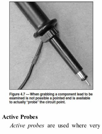
Active ProbesActive probes are used where very

low loading on the circuit is necessary.Quite often they have a field effecttransistor (FET) connected to the probetip, which means the tip has a very highresistance and low capacitance. Theyare, of course, more expensive andusually mate only with specificoscilloscopes for which they weredesigned. Active probes typically havean additional advantage of includingautomatic calibration. Since an amplifieris located in the tip, quite often this sortof probe has an extended bandwidth ofseveral hundred megahertz.

High Voltage ProbesHigh voltage probes are used when

the normal voltage limits for a passiveprobe are too low for the circuit underobservation. Most passive probes usedto be rated at 400 to 500 V (thinkvacuum tube transmitters), but today it isnot uncommon to see a probe rated atonly 200 V or even lower, matched tosolid state circuits. The key feature of ahigh voltage probe is safety — the probebody is designed to keep your handremoved from the high voltage.

Occasionally the probe connectingcable is made much longer, for the samereason — to keep your hand out of thecabinet or chassis containing the highvoltage circuits. Most high voltageprobes match a specific manufacturer’s

oscilloscope model and they generallyare not interchangeable.

Current ProbesCurrent probes are also generally

matched to a specific manufacture’soscilloscope model or models. Thecome in two types — ac (alternatingcurrent) only and dc (direct current). Inboth cases the bandwidth tends to belimited.

AC-Only ProbesT h e ac-only probe is simply a

transformer. In Figure 4.8 the twosections shown are basically thetransformer core, with the fixed primary

wound around the upper section. Therectangular slot is where the wirecarrying the current is placed. Squeezethe handle and the two sections open in ascissors mechanism. Insert the wire andthe transformer now consists of the fixedsecondary winding and the wire(primary) of the transformer.

Almost any wire that fits in the probejaws can be sensed, so the distance ofthe conductor from the metal core varies.Therefore the amplitude of the currentseen on the scope is not very accurate,but within the probe bandwidthlimitation the waveform is accurate.

Often an amplifier is included in theprobe handle so the connecting cablecarries signal information to the scopeand power for the amplifier to the probe,along with control signals to the probeamplifier.

DC ProbesA dc probe usually uses a Hall

Effect sensor. This is a solid-state

device that detects a magnetic field andproduces a (generally) minute outputvoltage in response to the field. Figure4.9 is a generalized curve of a HallEffect device. As you can see it has alimited range, so the magnetic field fromthe current being sensed must fall in thisrange or the sensor will go intosaturation, distorting the displayedcurrent waveform.

A block diagram of the dc currentsensor is in Figure 4.10. The electronicsare built into the probe, which resemblesthe ac-only current probe physically butuses the Hall Effect sensor instead of atransformer winding. Again, theamplitude of the current sensed may not

be very accurate, due to varying wirepositioning, but the waveshape as seenon the scope is accurate as long as thecurrent probe is being used within itsamplitude and frequency limits.

One More Probe Type forHams

Years ago, when amplitudemodulation was the most popular voicemode, amateurs built an RF detector asan oscilloscope probe add-on. Shown inFigure 4.11, this is nothing more than adiode detector that recovers the

amplitude modulation of a transmitter.This diode generally is germanium —the 1N34 being the most popular —since germanium diodes have a lowerjunction voltage than silicon. Today sucha probe is still useful for an AM signal,but not very useful for SSB. However itis very handy to see the keying envelopeof a CW transmitter.

Chapter 5

Scope Sections inDetail

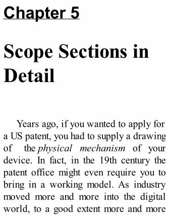
Years ago, if you wanted to apply fora US patent, you had to supply a drawingof the physical mechanism of yourdevice. In fact, in the 19th century thepatent office might even require you tobring in a working model. As industrymoved more and more into the digitalworld, to a good extent more and more

inventions were based on mechanismsthat did not exist physically, but weremade up of software programs.

At first the US patent office wouldsay “no way.” But as their requirementsand their understanding increased, as didthe digital abilities of patent applicants,the laws and rules changed. The officestarted to grant US patents on devicesthat were at least in part constructed insoftware.

We have a similar situation here. Toexamine the critical sections ofoscilloscopes, we use names of thesections that relate to hardware-onlyconstruction. But just about everysection can be constructed in either

hardware — with its advantages andlimits — or in software withcorresponding advantages and limits, orboth.

As this chapter goes through thescope sections, it will generally discussa hardware version of each section and asoftware version. Hardware scopes arestill being sold in large numbers,especially where reasonably goodperformance is desired at a lower cost.Both hardware and softwareimplementations — and combinations ofboth — have advantages anddisadvantages.

Functional Block DiagramUsually, for a piece of electronic

equipment, the block diagram that mostpeople are familiar with shows how thevarious hardware blocks areinterconnected. The functional blockdiagram of an oscilloscope in Figure5.1 shows how the various functions areinterconnected. The diagram includesboth straight hardware-implementedoscilloscopes and the variousconfigurations of digital signalprocessing based oscilloscopes.

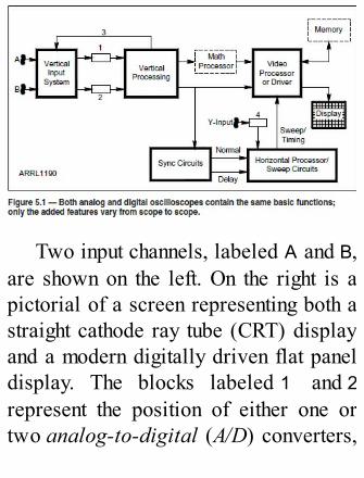
Two input channels, labeled A and B,are shown on the left. On the right is apictorial of a screen representing both astraight cathode ray tube (CRT) displayand a modern digitally driven flat paneldisplay. The blocks labeled 1 and 2represent the position of either one ortwo analog-to-digital (A/D) converters,

as found in a digital scope. Theadditional A/D converter, labeled 4, isdiscussed later in this chapter. Thedotted section labeled MATHPROCESSOR is found in many digitalscopes that use a microprocessor or arePC based. As long you have thecomputing power, the ability to dosimple and advanced calculations andmeasurements on input waveformscomes almost free!

The other box shown in dotted formrepresents data MEMORY. This is againan almost free function, available withdigital processing. At the bottom of thefigure, the concept or idea of the SYNCCIRCUITS block remains the same for

old and new analog oscilloscopes anddigital oscilloscopes, but theHORIZONTAL PROCESSOR/SWEEPCIRCUITS block is very much differentbetween the two technologies.

Vertical FunctionsChapter 6 will discuss in detail the

various input modes available in manyoscilloscopes. The correspondingfunctions are shown in Figure 5.2. In astrictly analog oscilloscope, the twomain blocks are a set of very precise —the degree of precision depending on thecost of the scope — analog amplifiers.They are designed to keep an exact

amplification factor and have low dcdrift.

This input mode control has fourchoices — A, B, ALT and CHOPPED.Details of ALT (alternate) and CHOPPEDare discussed in Chapter 8. Below the

control block are pairs of controls, onefor each input channel. POSITION movesthe trace up and down and VERTICALSCALE sets the gain — 10 mV/cm(millivolts per centimeter), 0.1 V/cm, 10V/cm and so on. But after these there is avariable calibration control (VERTCALCALIBRATE) that allows you to set ascale in between the fixed values. Oftenthis causes a problem. If this control isnot turned to one end — its CALIBRATEposition — the vertical scale is notcorrect. To add further flexibility, the X10 control changes the scale by a factorof 10 — usually used in conjunctionwith the X 10 switch on the probes.

In a digitally implemented scope, the

first block is a set of analog amplifiers,feeding either one or two A/Dconverters (blocks 1 and 2). With a dualchannel scope you would expect to seetwo converters, but if the scopebandwidth is low enough or the A/Dconverters fast enough (see Chapter 8 onscope specifications) just one A/D maybe shared, alternately convertingchannels A and B. After this conversionthe vertical processing is strictly digital,and there may be a feedback loop(shown here as 3) to stabilize the analogamplifiers.

On the right of the figure is the outputto the video processor or displaysystem. The second functional output (TO

MATH PROCESSOR) represents theoutput to the various measurement andmath functions that may be done beforeor on the displayed waveforms.

Horizontal Processor andSweep Circuits

The classic oscilloscope explanation,dating back to the original scopes in the1930s, had a diagram for the horizontalsection consisting of a sweep waveformsuch as that shown in Figure 5.3. Avoltage is applied to the horizontalplates of a CRT, and by increasing thevoltage the trace on the screen movesfrom left to right. At the end of the trace

the input signal to the vertical section isblanked, and the short section of thewaveform, labeled RETRACE, brings thetrace on the screen back to the left side.

Whether digital or analog, today’sscopes look functionally like the blockdiagram in Figure 5.4. A multipositionswitch sets the sweep rate (1 µs/cm, 10µs/cm, 5 ms/cm as examples). Just as inthe vertical section, a calibration controlmay be used to set sweep rate values inbetween the fixed sweep settings. Butonce again, when a calibration control ispart of the scope, it has to be set to the

calibrated setting (usually marked at oneend of the control) for the fixed values tohold. In addition, for convenience, oftena switch labeled X 5 (times 5) or X 10(times 10) is supplied.

Two inputs are shown from the SYNCsection. The NORMAL input usuallytriggers — starts — the sweep. Morecapable scopes provide a delayedsweep. As shown in Figure 5.5, a bugappears on the screen, intensifying thevideo at the point you pick past the startof the displayed waveform. Forexample, suppose you want to get a goodlook at the fall time of your Morse codekeyer waveform when sending a stringof dots.

You would set the main sweep atperhaps 100 ms/cm to show at least onecomplete dot, both the rise and fall ofthe voltage. Now you would move thebug to the falling edge (Figure 5.6),select a faster sweep rate (perhaps 10µs/cm) for the delayed sweep, and putthe delay sweep on. At this point youwould see the falling edge, at the fastersweep rate you selected, thus allowingexamination of this edge in more detail.

Some scopes provide an additionalinput to the HORIZONTAL PROCESSOR.There are several measurements whentwo voltages are compared (see Chapter7) against each other. One voltage inputis sent to the vertical axis through

Channel A or Channel B and the otherinto the horizontal axis through the Y-INPUT. In this case no sweep voltage isused. This Y-INPUT goes directly into thehorizontal section of an analog scope butmust go through an additional A/Dconverter (block 4) in a digital scope.

Most of the preceding explanationappears to apply only to analogoscilloscopes, but it also applies todigital oscilloscopes. As you will see ina following section on the VIDEO

PROCESSOR AND DRIVER, the voltagevalues sent to the vertical section areread out of memory starting at thememory location that corresponds to thetime of the sweep start, and read out at arate corresponding to the sweep rateselected. Instead of controlling analogcircuits, the controls described in Figure5.4 are actually software commands toset the speeds and functions.

Sync CircuitsPerhaps the most important parts of

any oscilloscope are the synchronizationcircuits. No matter how high thebandwidth, no matter how good the

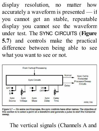
display resolution, no matter howaccurately a waveform is presented — ifyou cannot get an stable, repeatabledisplay you cannot see the waveformunder test. The SYNC CIRCUITS (Figure5.7) and controls make the practicaldifference between being able to seewhat you want to see or not.

The vertical signals (Channels A and

B) are sent to the sync processor. In ananalog system, this block is a set ofcomparators, trigger circuits, time delaycircuits, and pulse generators. In adigital scope the same function iscarried out by examining the stored data— in other words the incomingwaveform has been stored in a digitalmemory, and the values processed.

Whether the controls shown areactually physical switches and variableresistors or software commands, theireffect is the same. The input to the SYNCCIRCUITS comes from the verticalprocessing channel. A selection is made— Channel A, Channel B or an externalsignal through a separate connector. In adigital system this external connectorwould go to a Schmidt Trigger circuit orother circuit to result in a squared-offdigital pulse.

The operation of the SYNC VOLTAGEand SYNC SLOPE controls is illustratedin Figure 5.8. The various combinationsshown are:

A — positive voltage (value selectable),positive (rising) slopeB — positive voltage, negative (falling)slopeC — Zero crossing voltageD — negative voltage, negative slopeE — Negative voltage, positive slope.

Since the voltage selection isvariable, this set of controls usuallyallows you to set the sweep trigger pointto any point on the incoming waveform.

The remaining controls — SYNCDELAY a n d DELAY TIME — werediscussed in the preceding section. Thelocation of the bug is set by the DELAYTIME control and expanding to the delay

point (turning it on and off) is controlledby the SYNC DELAY switch.

There are two outputs. The NORMALoutput provides the start point in time forthe sweep, and DELAY output positionsthe bug. When delay sweep is turned on,the delay output provides the sweep starttime. Keep in mind that this descriptionis of the functions; how the hardware inany one scope actually does this varieswith the scope design.

Video Processor and DriverThere is a considerable difference

between the hardware and operation ofthe VIDEO PROCESSOR or DRIVER in the

classical analog oscilloscope and thehardware and operation in a digitalscope. Analog scopes are still readilyavailable and are often selected for thesimplicity, lower cost and widerbandwidth for the cost. A version of theclassical analog video section anddisplay is sketched in Figure 5.9. Thevideo from the VERTICAL PROCESSINGblock simply goes to a video amplifier,one that provides symmetry — theability to drive both positive andnegative with respect to a reference suchas ground. This amplifier is connected tothe vertical plates and thus provides thevertical deflection on the screen.

T h e HORIZONTAL

PROCESSOR/SWEEP CIRCUITS alsorequires a symmetrical amplifier,feeding this direct analog sweep voltageshown in Figure 5.9. This signal movesthe beam horizontally across the screen.The other signal is a blanking pulse, forthe duration of the retrace time in Figure5.3. During this period, as the tracemoves back to the left side of the screen,the blanking pulse puts a bias on the gridshown in Figure 5.9 that cuts off thevideo — thus no retrace is seen on thescreen.

Digital oscilloscopes, althoughfunctionally very much identical, operatecompletely differently on a hardwarebasis. There are two general

configurations — a self-containeddigital scope, and one that plugs into anduses a personal computer or other digitaldevice such as an iPad for calculationsand display of the traces.

Figure 5.10 represents this functionalconfiguration. It is based on storing theincoming waveforms in digital memoryafter they have been converted fromanalog voltages to digital words in thevertical input system. How data is storedin memory to be displayed is verydependent on the particular hardwaredevice. In Windows PCs, video memorycan be a part of main memory or it canbe a separate, high speed memory bank

on the video card. Apple products havetheir own techniques, as do Android andother digital devices. However thewaveform storage concept can beunderstood by looking at Figure 5.11.

At the top is an analog waveform thathas been converted to a digital number

by the front end A/D converters. Each ofthese converted numbers become adigital word, and as seen at the bottomof the figure each corresponding storedvalue goes into a memory location. Allmemory systems have an address foreach part of memory, and in the figure aset of address starting at address 230through address 280 is seen to hold thestored values for one channel.

This is a very simple linear system,and various techniques for videocompression and memory locationselection are used to speed up videodisplay. Whatever the real storagetechnique used, these values can becommanded to set a vertical position on

the display screen as the horizontalprocessor provides a horizontal position— the horizontal processor provides theequivalent of a sweep. Call the sequenceof values quickly out of memory and youhave a fast sweep rate — say 10 µs/cm.More slowly and you have a slowerrate, say 100 ms/cm.

Thus the stored value provides thevertical position on the screen and rateand call-out speed from memoryprovides the horizontal timing andposition. In Figure 5.10, MEMORY isshown in a rectangle — it is actuallyintegral to the video processor.

What About Math?Earlier in this chapter there was a

statement that in a digital scope, mathcalculations come almost free — that is,no additional hardware is required.Looking at Figure 5.11 you can see howthe MATH PROCESSOR, also shown inFigure 5.10, can be used to find the peakvalue or minimum value, or to select allpoints and calculate an average — allbecause the data exists in memory. If theChannel A waveform is stored inmemory locations 230 to 280, and thechannel B waveform is stored inmemory locations 330 to 380, formingthe function A+B now requires only asoftware command to add the value in

memory location 230 to the value inlocation 330, the value in 240 to thevalue in 340, and so on. Since largeamounts of incoming waveform data canbe stored, much more complex mathfunctions, such as spectrum analysis, canbe done in software with the resultsdisplayed on the screen.

Does the Display TypeMatter?

Plasma, LED backlight, thin film … ahost of display types are available.However the display now has to bematched to the processor and not to theoscilloscope functions. This means that

the video card (or integral videosection), for example on a PC, ismatched to the display. If what is oftentermed the native resolution selected,the particular display used will notaffect the oscilloscope function.

There are, of course, severalpossible exceptions. If a digitaloscilloscope front end is mated with anolder personal computer using 640 ×480 resolution, your results may not beall they can be. Another possibleexception is the set of miniatureoscilloscopes that mate to smartphonesor tablets. Here the problem is not somuch display resolution — you won’tsee the difference — but the screen size,

even with a 8 or 10 inch tablet, mayrestrict what you can see.

StorageMost of the time the ability to store a

waveform on the screen is not ofprimary importance. There is one case,however, where it becomes veryimportant. In general an oscilloscope isused to look at repetitive waveforms.For a digital oscilloscope, memory isbuilt in. Looking again at Figure 5.11, ifthese memory locations represent a fullscreen of information, when memorylocation 280 is filled the entire set isnormally (and very quickly) cleared and

the new incoming waveform refillslocations 230 to 280. The processrepeats over and over, and storage of awaveform is not important.

There is one very important casewhere storage is required — when youwant to examine an transient effect thatonly happens once. Then you would liketo fill up 230 thought 280 and freeze —hold on to — the result. Again, thisability comes free with digitalimplementation.

There were and still are analogscopes with storage capability. Therethe storage is not in the circuits but in theCRT. By adding a mesh or screen justbehind the phosphor layer on the front to

the CRT and some unique electronflooding, the actual storage isaccomplished in the phosphor layer onthe screen. To see an example of thistechnique, set your Internet search enginet o typotron o r SAGE System Displayand you can see the details of oneapplication. These analog storagescopes were, of course, quite expensiveand very rare outside of industriallaboratories or military hardware.

No-Hardware ScopesSince some digital oscilloscopes

plug into a PC, and use the PC for all theprocessing and display, why bother with

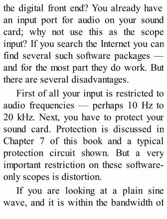
the digital front end? You already havean input port for audio on your soundcard; why not use this as the scopeinput? If you search the Internet you canfind several such software packages —and for the most part they do work. Butthere are several disadvantages.

First of all your input is restricted toaudio frequencies — perhaps 10 Hz to20 kHz. Next, you have to protect yoursound card. Protection is discussed inChapter 7 of this book and a typicalprotection circuit shown. But a veryimportant restriction on these software-only scopes is distortion.

If you are looking at a plain sinewave, and it is within the bandwidth of

the audio card, your results will bereasonable. If, however, you are lookingat a square wave, triangular wave or anyrepetitive waveform other than a sinewave, there will probably beconsiderable distortion.

Without getting deeply in to the mathto explain this, a technique known asFourier analysis shows that everyrepetitive waveform consists of a set ofsine waves, each at a multiple of thewaveform frequency and with a certainamplitude. As an example, suppose youwant to look at a perfect square wave at5 kHz. This square wave is actuallymade up of the addition of sine waves at5 kHz, 15 kHz, 25 kHz and other odd

multiples of 5 kHz — each with aprecise amplitude.

Since the no-hardware scope doesnot show sine waves above 20 or 25kHz accurately, instead of seeing aperfect 5 kHz square wave you couldsee a very distorted 5 kHz waveformwith rounded top and sloping sidesinstead of the nice, rectangular squarewave you expect. No-hardware scopesdo have their place in audio-onlyapplications. They are inexpensive(often implemented in free software) andfun — but don’t expect to use on in placeof a hardware-based scope.

Chapter 6

Input Modes

What you can see on youroscilloscope is controlled to a largeextent by what input modes areavailable, and the input modes in turnare controlled by — as you might guess— both circuit design and theoscilloscope controls available. Inaddition, the real-life designconsiderations that went into the scopeprovide further capabilities and

limitations.In this chapter, to illustrate various

points we will use pictures of vintageTektronix oscilloscope input modules.This series of scopes consisted of a baseunit with replaceable, often singlepurpose plug-in units for the front end ofthe scope. We will also look at today’smodern designs that have combined boththe capabilities and controls of the olderscopes — an objective which just wasnot reachable back in the vacuum tubedays.

As an example, suppose you need asingle, very high gain input capabilitywith very precise calibration. Anaccurate, high gain capability requires

accurate and long lasting calibration. Inaddition, extra bandwidth reduction maybe required to keep system noise fromcorrupting the waveform you wish tosee. Therefore, it is not just a matter ofdesigning a high gain input amplifier. Itmust be stable, have accurate and lastingcalibration, and exhibit a degree of noiseimmunity. From this point of view, thedesign of an oscilloscope front end isnot very much different from the designof a good preamp for your AmateurRadio receiver — low noise, properbandwidth, stable amplification and soon.

A number of amateurs discoveredthis similarity with later model Heathkit

oscilloscopes. Prior to the demise of thecompany, Heath offered a set of solid-state oscilloscopes with bandwidthsranging from 5 MHz to 35 MHz (andpossibly higher with some models.)Hams who bought and built these kitsdiscovered they were building circuits— and having to calibrate them — justas they would an amateur receiver.

Input ModesAs might be expected, in a

competitive world, differentmanufacturers pick and publicize theirscope capabilities with names that oftendo not match those of their competitor’s

capabilities for the same function. Hereis a list of common input modes undergeneric — commonly accepted —names. Most often when there are twoavailable input channels, they arereferred to as channel A and channel B.

Ground (reference) Ac Coupled (selectable

independently for each channel) Dc Coupled (selectable

independently for each channel) Inverted Differential (no ground reference) High Gain Fast Rise Time Dual Trace

A/B Alternate A/B Chopped A+B (A plus B) A–B (A minus B) High-Z (high impedance) Input 50 Ω Input Wide Band Digital Inputs Multi-channel Audio OnlySome of these input modes are fairly

obvious just from their titles; otherrequire a bit of explanation as to benefitsand limits.

Common Input SelectionsIndependent of the oscilloscope type

— hardware only, hardware andsoftware, and software only — there arealmost always three input selections.These are pictured in Figure 6.1, wherethe lever switch on the left hand side isused to select ac inputs only, dc inputsonly or a ground reference. The groundreference is used to set a baseline of 0 Vinput, so that everything seen after thatcan be referenced to this value(specifically this line as seen on thescreen.) The other two selections, accoupled and dc coupled, are exactlywhat their names imply.

Suppose you are looking at a

waveform that consists of a dc level of30 V, on top of which is riding a 1 Vsawtooth. By first selecting GND (theground reference) and positioning it atthe bottom of the screen you know wherethe vertical position of 0 V is. Next, byselecting DC (dc only) position, thewaveform will show up in its entirety,assuming you have the vertical voltagescale set high enough. However the 1 Vsawtooth will be very hard to measure.

Next when you select the AC (accoupled) position, the dc level

disappears and you can readjust thevoltage scale to better see and measurethe amplitude of the sawtooth.

These input selections are setindependently for each input channel —that is, there is another lever switch (notshown) for the second channel. Figure6.2 shows the on-screen controls of ascope using a personal computer, withthe coupling controls at the lower left.The input controls are duplicated foreach of the two channels.

Some oscilloscopes also provide anINVERTED selection that allows you todisplay a signal with low voltage at thetop of the screen and high voltage at thebottom. This is generally available when

the scope also has some sort of integralmath function.

Single Channel ModesDepending on the intended use, age

of the scope, and cost, someoscilloscopes provide specific

specialized features on either a singlechannel input or multiple channel inputs.Not all of these features are compatiblewith each other.

Previously we mentioned that highgain front ends may not be compatiblewith a system looking for highfrequencies. Where the best frequencyresponse is needed, manufacturers mayrefer to this characteristic as Wide Bando r Fast Rise Time. Figure 6.3 is thefront-end plug-in of a Tektronix scope ofa few generations ago, where the designwas optimized for fast rise time.

Although Wide Band and Fast RiseTime are similar, they are used andmeasured differently. Wide Band refers

to the highest frequency that displays(generally) at least 70.7% of the correctamplitude value of a sine wave. FastRise Time is important for digitalmeasurements only, and fast is incomparison to the rise and fall time of adigital pulse you want to measure.

Today the specifications of a scopewould tell you its characteristics in theseareas assuming the manufacturerincludes it in a full listing ofcapabilities.

While most scopes are designed tohave minimum loading on a circuit —that is the presence of the scope does notaffect the circuit performance — somescopes are specifically labeled High-ZInput. Normally the input of a moderatevalue scope would look like a 1 MΩresistor in parallel with 10 pF. A High-ZInput would be several 10s of megohms,but the input capacitance is stillgenerally at least 5 pF. Usually the High-Z Input requires a special probe,matched to the scope design.

For work on transmission lines,where any impedance mismatch mayaffect the measurement, there arespecialized scope whose inputs look

like a pure 50 Ω resistor. Thus they canact as a matched load (for very lowpower levels) on a port or splitterattached to the line.

Dual Channel InputsWhile the early oscilloscopes

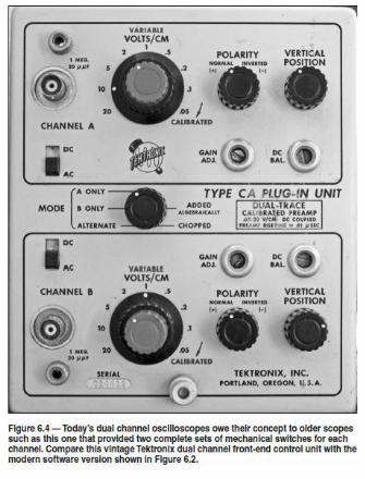
described in Chapter 1 concentrated onallowing a single signal to be seen,scope capability has grown to include,for just about all models, a two-channelor dual-trace input. Again, using a verypopular obsolete Tektronix plug-in frontend as an illustration, Figure 6.4 showsthe identical controls for the twochannels. A five position MODE switch

selects the channel or channels to bedisplayed.

The first two positions allow you tosee one channel only, either A or B. Thethird position, ALTERNATE, can be verymisleading. What you see depends on thesweep trigger section (as described inChapter 5). If the sweep is triggered byone channel and that channel only, thehorizontal position or relative timing ofthe second channel may not be what youobserve.

The result of modern dual-channelinputs is illustrate in Figure 6.5, where asquare wave is shown in channel A,triggered by the square wave, with atriangular waveshape in the lower trace.Each trace provides its own trigger, soalthough you see both in stable positions,

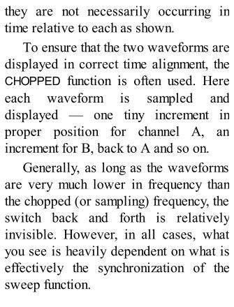
they are not necessarily occurring intime relative to each as shown.

To ensure that the two waveforms aredisplayed in correct time alignment, theCHOPPED function is often used. Hereeach waveform is sampled anddisplayed — one tiny increment inproper position for channel A, anincrement for B, back to A and so on.

Generally, as long as the waveformsare very much lower in frequency thanthe chopped (or sampling) frequency, theswitch back and forth is relativelyinvisible. However, in all cases, whatyou see is heavily dependent on what iseffectively the synchronization of thesweep function.

The fifth position on the MODEswi tch, ADDED, is one example ofmathematically combining the twooutputs, in this case a simple addition.

Dual Channel withArithmetic

The simple arithmetic function labelshown in Figure 6.4 (ADDED) impliesaddition. However, both channels havePOLARITY (NORMAL or INVERTED)selectors, which simply switch ininversion of the either or bothwaveforms. This function, incombination with the ADDED(ALGEBRAICALLY) mode position meansthe waveforms A and B can becombined in four possible ways: A+B,A–B, B–A and finally –A–B.

A newer Tektronix oscilloscope,

shown in Figure 6.6, has a controllabeled MATH near the center of thefigure. Here a number of combinationsof signal (and calculations) may beselected.

One of the most valuable modes fordesign and troubleshooting modernelectronics, especially where digitaldata lines are used, is the differentialmode. The arithmetic described in theprevious example has an inherentcharacteristic. For example A+B isreally (A as compared to ground) + (Bas compared to ground). What happens ifneither signal is referenced to ground,but they are referenced to each other? Infact introducing the ground connection

may show noise and other extraneoussignals that really do not exist on the lineunder test.

Figure 6.7 is a block diagram of atypical balanced line driver — it hasfour independent sections — A, B, C,and D. Looking at section A at the topleft, a data waveform is connected to pin1. The output is balanced and connectedto pins 2 and 3. This output is notreferenced to ground, but as shown oneis the nominally labeled positive dataoutput line and the other is the negativeor return.

There are many such integratedcircuits used with variousconfigurations, but the common

characteristic is the lack of a groundreference. At the other end of the line acomplementary data receiver has twoinputs per channel, and the output of thecircuit is a single data steam for thechannel.

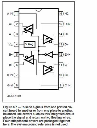
In a modern piece of electronics,where RF may be found, a designer maychoose to send data from one printedcircuit board to another using adifferential driver and receiver tominimize RF pickup with respect toground.

Again using an old Tektronix scopeas an illustration, Figure 6.8 shows ahigh gain differential front end.Tektronix actually made two suchdifferential front ends, this one calledHIGH GAIN and a second called WIDE-BAND.

Special ModesWhen you want to look at logic

signals, a dual channel capability maynot be enough. There are a fewmanufacturers of four channel scopesand possibly models with even more.

A newer approach is illustrated inFigure 6.9. As shown, the top two

regular channels are not connected toany signals. This scope has four logicsignals only input wires. In the figure,the four lower traces are inputs on theseconnections. Any one of these inputs canbe selected as the sync source, whichgives a good degree of flexibility inchoosing what to look at.

One very specialized front end for ascope, which has no front end, is thesoftware-only scope discussed inChapter 7. This scope uses yourcomputer and audio card. As a result its

bandwidth is limited to the audiofrequency range only — perhaps a fewtens of Hz to 20 kHz. Several versionsof the software are available online,mostly without charge. Although a directconnection to a sound card is possible,most users follow the online directionsto build a small protection circuit for thesound card. One such circuit is includedin Chapter 7.

Chapter 7

Let’s Put a Scopeto Work

Oscilloscopes are generally used forone of three types of measurements:amplitude (voltage), duration or time(frequency), and calculations. Mostolder scopes did not have the ability todo calculations, but as discussed inpreceding chapters, as long as you haveinformation in digital form and are using

a digital processor (in other words asmall computer), the oscilloscope cando a variety of calculations.

Amplitude MeasurementsWhen most people think of using an

oscilloscope, they envision a screenwith a plot of the amplitude or voltage ofa signal on the vertical axis of a screen,along with time on the horizontal axis.To make this primary plot on thedisplay, there are several steps you haveto take. It is very possible to overlookone of these steps, in which case thedisplayed waveform may mislead youand not represent the true picture of the

signal.First pick a voltage scale, and if

there is a variable scale control, makesure the voltage scale selection switch isin the calibrated position. Looking atFigure 7.1 you can see scale selectionswitches for channel 1 and channel 2.Notice that the center knob (labeledVAR) for channel 1 is in the fullclockwise position, corresponding to thecalibration position on the panel. TheVAR knob for channel 2 is not in thesame position, so as a result the voltagescale selected for channel 1 is correctbut the scale selected for channel 2 isincorrect. It is very easy and verycommon to overlook checking this

setting.Check your probe compensation.

Compensation, as noted in a priorchapter, only holds for the X10 setting onthe probe switch. If you are lookingprimarily at sine waves and RF, it isdoubtful that (except for extrememaladjustment of the compensationscrew) this adjustment will make muchof a difference. Digital signals are adifferent story — just look at Figure 7.2!With compensation maladjustment,square waves, pulses, sawtooth andother linear waveforms may be shownfar from their true waveshape.

Set up a zero reference. Most scopeshave an input setting marked GROUND orGND; it is difficult to make ameasurement if you do not have areference.

Now you are in a position to make avoltage measurement. Count the numberof centimeters (cm) on the vertical scale.You may have to move the horizontalposition control (if there is one) orchange the trigger point to get a goodmeasurement on the subdivisions of thegraticule. Multiply the number of cm bythe voltage scale and you have yournumber — almost!

Now go back and look at your probe.Do you have it in the X10 position? If so,multiply your previous reading by 10!

A word of caution: It is easy to getconfused when you compare a readingfrom a voltmeter with the measurementyou just took on a scope and see that they

are different and assume that either thescope or the voltmeter is in error.Remember that most voltmeters measureRMS (root-mean-square) values, but youmost probably just measured a peak-to-peak value on the scope. To get anequivalent value, take the peak-to-peaknumber, divide by 2 to get the peakvalue, and then multiply the peak valueby 0.707 to get RMS. This simpleconversion holds only for sinusoidalwaveforms.

Another thing to keep in mind whenmeasuring waveforms near the upperlimit of the scope’s bandwidth is that thegenerally accepted figure for bandwidthis the frequency where the measurement

is off by 3 dB in voltage. That is, thewaveform may show 3 dB lower than itactually is.

Alignment with a Sweep GeneratorOne very common voltage

measurement using a scope is thealignment of an IF strip in a receiver orthe measurement of an RF or audio filter.That requires a signal generatorproduces a signal at the frequency orfrequencies of interest, or a sweepgenerator (a signal generator that sweepsits output signal over a range offrequencies).

As an example, assume the OBJECTUNDER TEST in Figure 7.3 is a filter

with a center frequency of 1 MHz. If wewanted to see the filter response from900 kHz to 1.1 MHz, the sweepgenerator would be set up for its outputfrequency to vary from the lower 900kHz limit to the upper 1.1 MHz limit. Asthe frequency changes, the sweep outputvoltage also changes, so every point onthe horizontal axis corresponds to afrequency in the swept range. The RFvoltage goes into the filter and the outputof the filter goes to the vertical input ofthe scope.

The net result is a plot seen on thescope display that shows the filtercharacteristics over frequency. SeeFigure 7.4 for an example filter

response plot. If the actual test were runat RF, a small diode detector (Figure7.5) would be placed in series with theVERTICAL INPUT so that the actualvertical input would be dc. The dcvoltage value at any frequency woulddepend on the filter characteristic.

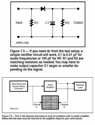
Amplifier LinearityFor checking the “goodness” of an

audio amplifier, its linearity can beobserved by the system shown in Figure7.6. The input to the amplifier isconnected to channel A and the output tochannel B. The usual test would use sinewave inputs, but a further, more rigoroustest would use a square wave, triangular,or sawtooth input. The sine wave couldbe at any frequency within the capabilityof the amplifier, but the square wavefrequency should be limited toapproximately 1/3 the upper frequencylimit of the amplifier.

Although it is customary just tocompare the input and output “by

eyeball,” a more interesting test is to setthe voltage scale on both channels sothat they both give the same verticaldeflection. Then set the scope to the A–B (A minus B) position. On the screen, ifthere is no phase delay through theamplifier (an impossibility) the two sinewaves would subtract out, but in thepractical case, with no distortion, thedisplay would show the phase shift inthe amplifier.

Transmitted AM waveformFor many years the classic use of an

oscilloscope in the ham shack was toobserve (and set) the modulation levelof an AM transmitter. Most old ARRL

Handbooks and reference volumesdevoted at least one page to the outputRF waveform as seen on a scope undervarious conditions. As an example,Figure 7.7A shows a properlymodulated AM transmitter and Figure7.7B shows one with overmodulation.

These pictures still hold for simple,older AM modulated transmitters. Manynew ham rigs include an AM capability,with the ability to apply various degreesof speech processing and compression.Often, as seen on an oscilloscope, thetransmitted signal will look fine — suchas in Figure 7.7A — but on the airreports will be very mixed and negative,because it is often very difficult to see

the result of processing in this simplescope test.

To see the RF output from atransmitter, it is usually not necessary tobuild a sampling circuit that physicallyconnects to the signal on thetransmission line; usually — since theSWR on a coaxial line is rarely 1:1—you can simply either wind a loop of

wire around the antenna feed line in thestation or tape a 6 or 12 inch piece ofwire along the feed line. Usually therewill be sufficient pickup to see thetransmitted RF waveform

SSB TestingObserving a single-sideband signal

can also be interesting but misleading. Abit of a voice conversation on 40 metersis captured in Figure 7.8. A moremeaningful view is Figure 7.9, whichshows a well-adjusted 75 meter SSBtransmitter modulated by a single tone.For comparison, Figure 7.10 showswhat the transmitter output looks likewith a single tone but with a carrier that

is not fully suppressed. In other words,the transmitter is not putting out a single-sideband signal but a sideband withsome carrier.

Again a word of caution — manypictures have been published that showwhat a good SSB signal should looklike. However, just as with an AMtransmitter, it is quite possible to have abeautiful picture but get very poor on-the-air quality reports due tomaladjustment of the speech processor.

Also see the section on measuringPEP output power later in this chapter.

CW TESTINGThere are several measurements that

an oscilloscope can make to check thequality of your CW signal. The first, andmost basic, is to look at the amplitude of

the transmitted dots and dashes. Do theystay constant within the period of a dotor dash? While this seems like afundamental requirement, did you everhear someone transmitting a signal that,if an honest report were given, wouldwarrant a tone value (the T in RST, 1 to9) of less than T9? Older transmitters,especially with poorly regulated powersupplies, often suffered from thisproblem. If the transmitted waveformwere examined on a scope while aseries of dots or dashes were keyed, youcould easily see a change in amplitudeduring the period of a dot or dash.

A good keying waveform is shown inFigure 7.11. The top trace is the keyclosure and the bottom the transmittedwaveform. Notice the waveform lags thekey closure by a fixed period; this isnormal. The waveform has a gradual

build-up and decay. Compare this withFigure 7.12, where the transmittedwaveform is has sharp edges whichresult in a broad signal — in otherwords key clicks up and down the band.

Figure 7.13 shows another problemthat can be seen with an oscilloscope:shortening of the first dot or dash whenusing break-in. Sometimes this effect innot noticeable and sometimes it has thereceiving operator scratching his or herhead and asking “What was that firstletter?” This effect is particularlynoticeable with high-speed CW and fastbreak-in.

To examine the transmitted waveformclosely at the beginning and end of a dot

or dash you will want to set up a veryfast horizontal scope scan speed. Thisrequires you to use a delayed trigger asexplained in Chapter 5. The horizontalscan speed is set to show one or moredots or dashes and the bug, representingthe position of the delayed sweep, or theSWEEP DELAY TIME, moved onto theleading or trailing edge of the dot ordash. The time base for the delayedsweep is set to a high speed and thedelay sweep turned on. You will then beable to examine the leading or trailingedge of the dot or dash in great detail.

Digital SignalsWith the popularity of digital

equipment, some oscilloscopemanufacturers have added inputconnections specifically to allowviewing of digital signals, and usually abinary number equivalent number (4, 8,and 16) of them simultaneously. As anexample the Oscium scope shown inFigure 2.14 in Chapter 2 has four digitalinputs. There may be, depending on thespecific scope design, advantages anddisadvantages to these inputs.

Certainly having a number ofsimultaneous inputs (more than two) isan advantage. If the design connects yoursignals directly into digital logicelements, without using an A/D (analog-to-digital) converter, higher speed logic

circuits may be monitored. However,this direct connection means that theactual waveform is not shown; just logic1s and 0s are on the screen.

A possible further limitation of adirect digital connection is theallowable input voltage range. Whilemost common digital circuits operatebetween 0 V (or perhaps minus a fewvolts, down to –12 V) and up to +5 V (orpossibly as high as +20 V), theallowable input voltage range of directdigital connections are very muchrestricted as compared to the allowablevoltage range using the usual dual-channel, probe connected inputs.

The oscilloscope bandwidth can also

provide a misleading but importantlimitation, when the usual ChannelA/Channel B inputs are used. Asdiscussed in Chapter 5, signals such assquare waves and repetitive pulses aremade up of sums of sine waves. Figure7.14A shows a square wavesuperimposed on a sine wave of thesame frequency. Figure 7.14B shows thesame square wave, but this time the sinewave is added to a second sine wavethat is at three times the frequency. Thisthird harmonic sine wave amplitude hasbeen multiplied by a number less than 1.

Figure 7.14C shows the result if theoriginal sine wave, a second one ofthree times the frequency and a third one

of five times the frequency. Finally,Figure 7.14D shows the result of addingthe original, three times, five times andseven times the original frequency —each harmonic component has acalculated multiplier. Thus as you addmore and more odd harmonic sinewaves, the result looks more and morelike a rectangular square wave.

Now suppose you have a squarewave input at, for example, 10 MHz. Ifyour scope bandwidth is only 40 MHz,the third harmonic of the 10 MHz input(30 MHz) will get through, but the fifthharmonic (50 MHz) and seventhharmonic (70 MHz) components will beattenuated. Then the square wave you

might see could look more like the onein Figure 7.14B — that is the squarewave would be rounded at the rise andfall, and not flat at the top and bottom.

Fortunately the situation is not totallylike this, because a scope’s bandwidthdoes not fall off a cliff. A 45 MHzbandwidth means the response to a 45MHz sine wave would be about 3 dBdown in voltage, so some of the 5thharmonic energy would get through.

The net result is this: While a scopebandwidth specification tells you justhow high in input signal frequency youcan go suffering only a 3 dB loss, thesame bandwidth is a limitation of thefidelity of the digital signals; they may

not be seen with their properwaveshape! This phenomenon isdiscussed further in Chapter 8, wherespecifications for a scope’s verticalchannel rise and fall time are noted.

Another consideration that can be agreat advantage when viewing digitalsignals is the ability to see one-timeaction. Sometimes, for unanticipatedreasons, something will happen veryquickly, and your eye will not catch it.Here the ability to set an oscilloscopeinto a storage mode, where the trace istriggered just once and the result left onthe screen, can be invaluable. Again, aspointed out before, digital storagescopes retain the input data in memory,so that the ability to store one or moretraces is built-in for examination atleisure.

RF Detection

As mentioned in the precedingsection, oscilloscope bandwidth is not acliff. A bandwidth specification such as50 MHz does not mean that you will seeno signal above this frequency. It doesmean that this is the frequency,commonly noted as 3 dB down, abovewhich waveforms will not be seen withtheir true amplitude. It is not unusual tobe able to see signals at twice or threetimes the rated bandwidth, but theamplitude will likely not be accurateabove the rated frequency.

If you are trying to do this, rememberto check the probe setting and perhapsplace it in the X1 position instead of X10.A second important point, especially

with RF at any time, is that you may notknow the actual voltage of an RF signal.Some caution is required so theoscilloscope or the probe is notdamaged by overvoltage.

As noted previously, to pick up RFfrom a transmission line often it is notnecessary to connect to the transmissionline. A loop of several turns around acoaxial line, especially where the SWRis not close to 1:1, may be sufficient. A6 or 12 inch piece or wire taped to thetransmission line may also work.

When you want to see the modulationenvelope of an RF signal, a simplediode detector connected to the RFpickup device will suffice. Figure 7.15shows one such circuit. You may have toincrease or decrease the value of the 50pF output capacitor, depending on thebandwidth of the modulation. Agermanium diode, the venerable 1N34 isshown. A germanium diode here has theadvantage of more sensitivity since the

voltage drop across it is less than asilicon diode.

Time (Frequency)Measurements

In the normal use, the horizontal axisof an oscilloscope is set so the tracemoves from left to right at the set timebase rate — but as you can see from thetitle of this section this time base or scanrate represents both time and frequency.For any periodic wave, the relationshipis f = 1/T, where f is frequency and T istime. As an example, a 1000 Hz sinewave — that is, 1000 alternations persecond — traces out 1000 sine waves

per second. The duration or period of asingle sine wave is 1/1000 of a second.To see the waveform of interest, youhave to set the time base so thewaveform is visible. Fortunately youdon’t have to know the waveformfrequency accurately; you can put thewaveform on the screen and vary thetime base until you get a satisfactorypicture.

Using the Time BaseAll oscilloscopes have a TIME BASE

control, which is calibrated in units oftime per division. For example, inFigure 7.16 the TIME BASE control(which is labeled TIME/DIV) is set to 0.5

ms (one half millisecond) per division.Therefore, if the graticule on the screenhas 10 major divisions across, it takes10 times 0.5 ms to sweep across thescreen, or 5 ms.

As another example, a 400 Hz sinewave has a period of (T = 1/f) or (T =1/400). Therefore one complete sinewave takes 1/400 of a second or 2.5 ms.Since the horizontal scan rate or timebase is set to 5 ms for a complete scanacross, 5/2.5 = 2, so there will be twocomplete sine waves showing.

However, just as with setting thevertical channel sensitivity, it is veryeasy to make a mistake here. Look just to

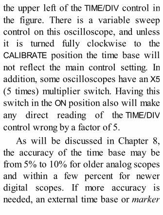
the upper left of the TIME/DIV control inthe figure. There is a variable sweepcontrol on this oscilloscope, and unlessit is turned fully clockwise to theCALIBRATE position the time base willnot reflect the main control setting. Inaddition, some oscilloscopes have an X5(5 times) multiplier switch. Having thisswitch in the ON position also will makeany direct reading of the TIME/DIVcontrol wrong by a factor of 5.

As will be discussed in Chapter 8,the accuracy of the time base may befrom 5% to 10% for older analog scopesand within a few percent for newerdigital scopes. If more accuracy isneeded, an external time base or marker

generator can be used. There aregenerally two ways the generator cangive you a better time base reading. Thefirst is to put the waveform you aremeasuring into one channel and the timegenerator into a second, superimposethem and do your measurement.

The second way to is to use theVARIABLE SWEEP control mentionedbefore. Put the marker generator into onechannel and use the VARIABLE SWEEPcontrol to make the marker pulses lineup with the divisions of the graticule onthe screen. Now you can count thedivisions directly, because they havebeen calibrated by the marker generator.

Lissajous PatternsAn older way to use a scope to

measure frequency uses a known,calibrated sine wave generator. As seeni n Figure 7.17, the known frequencysource is connected to either the verticalinput or the horizontal input and theunknown into the other input. When theknown generator is set to an exactmultiple of the unknown frequency, oneof the patterns shown in the figureresults. The number of lobes is equal tothe frequency ratio. This technique datesback to before inexpensive digitalfrequency counters were available, butis cost free and is an additional use foryour scope.

Gadgets to AddThere are any number of small (and

not-so-small) circuits you can build toextend the use of your oscilloscope.Some are very quick to build and use —for example, if you have a sine wavegenerator with a known frequency

calibration, just add a resistor in serieswith an unknown capacitor or inductorand you can measure the voltage acrossthe unknown component and thencalculate its value.

Diode TesterA very popular accessory is shown

in Figure 7.18. It is a diode tester, andwhen the diode is operating properly thepattern of Figure 7.19 results. Notice theapproximately 0.6 V flat horizontal lineon the display. This was a silicon diodeunder test; it takes approximately 0.6 Vforward bias before it conducts. Thesame circuit can be used to check thebase-emitter and base-collector

junctions of transistors and several othertypes of diodes.

High Frequency AmmeterAn oscilloscope can be very useful

as an ammeter. At frequencies above 60Hz power line ac, ammeter performancefalls off in a generally unknown manner.Chapter 6 included a discussion of using

a dual channel scope in a differentialmode. By placing a very smallresistance in series with the linecarrying the current, and placing the twoprobes at opposite ends of the resistor,Ohm’s Law will give you the current asthe voltage difference divided by theresistance. The frequency limit here isthe scope performance, which isobviously a lot higher than 60 Hz!

Sound Card ProtectionChapter 8 includes a brief discussion

of an interesting no-hardwareoscilloscope that uses your PC and thecapabilities of the sound card.Specifically, a version of oscilloscopesoftware is hosted on the PC. The inputis not through an analog verticalamplifier and external A/D, but throughthe A/Ds found on the computer’s soundcard.

Obviously the performance of thistype of scope is limited to the bandwidthof a typical sound card, perhaps 20 –20,000 Hz. Exposing your sound card toan outside signal can result in the loss ofthe card. A basic protection circuit for

this scope is in Figure 7.20. Using twosilicon diodes in series limits thevoltage into the sound card to about 1.2V, positive or negative. An optionalvoltage divider (a single variableresistor) is shown to adjust the inputlevel. In addition to the bandwidthlimitation, this type of system does nothave a high input impedance and caneasily load down the circuit under test.For an audio frequency scope tocompare amplifier input and outputsignals (in other words, look fordistortion), the price is right.

Scope Bandwidth ExtenderIf you have an oscilloscope with, for

example, a bandwidth of 10 MHz andwould like to examine a 28 MHz signal,you might be able to do it. If you couldconvert the 28 MHz signal down to afrequency below 10 MHz, that would beideal. This solution is not much differentthan the approach used in manyreceivers — heterodyning the signaldown to a lower frequency. One suchcircuit is shown in Figure 7.21(reproduced from Chapter 25 of the2 0 1 0 ARRL Handbook). This circuituses three transistors and a singleMiniCircuits SRA-1 mixer.

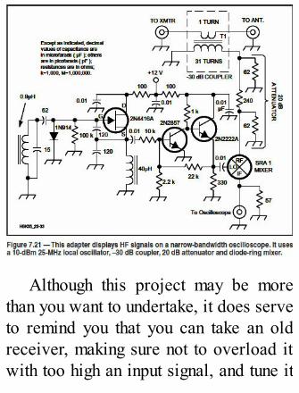
Although this project may be morethan you want to undertake, it does serveto remind you that you can take an oldreceiver, making sure not to overload itwith too high an input signal, and tune it

to whatever signal you want to examine.Connect your oscilloscope to the IFamplifier and you will get to view thehigher frequency signal. Remember,however, that the signal you see is nowlimited by the receiver bandwidth andnot the scope bandwidth.

Measure Your PEP OutputOne of the most perplexing questions

many hams ask, after they think about theFCC requirement of “no more than 1500watts PEP,” is “How can I measure it?”Just how much PEP (peak envelopepower) is my transmitter putting out?Even though you may be using one of the

many 100 watt output transceivers (perthe manufacturer’s specification) socommon on the bands, just how muchpower is coming out?

You can use a scope to get a fairmeasurement of this number, using thecalculation technique in Chapter 2 ofThe ARRL Handbook and describedhere, but you will have to exercisecaution so that you don’t damageyourself, your scope or its probe. Withhigher power transmitters you could beexposed to RF voltages in the 600 to1000 V range.

First connect your transmitter to 50 Ωdummy load through a coax T adapter.The load has to be resistive, with noinductance or capacitance.

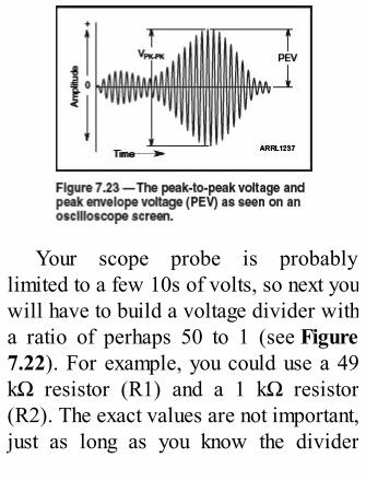
Your scope probe is probablylimited to a few 10s of volts, so next youwill have to build a voltage divider witha ratio of perhaps 50 to 1 (see Figure7.22). For example, you could use a 49kΩ resistor (R1) and a 1 kΩ resistor(R2). The exact values are not important,just as long as you know the divider

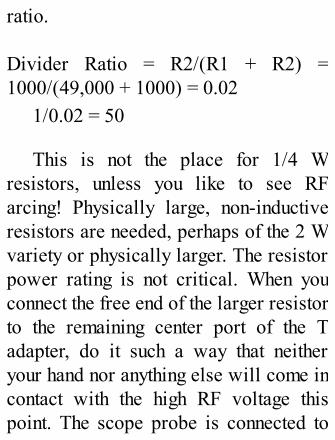
ratio.

Divider Ratio = R2/(R1 + R2) =1000/(49,000 + 1000) = 0.02

1/0.02 = 50

This is not the place for 1/4 Wresistors, unless you like to see RFarcing! Physically large, non-inductiveresistors are needed, perhaps of the 2 Wvariety or physically larger. The resistorpower rating is not critical. When youconnect the free end of the larger resistorto the remaining center port of the Tadapter, do it such a way that neitheryour hand nor anything else will come incontact with the high RF voltage thispoint. The scope probe is connected to

the junction of the two resistors and theprobe return is connected to ground.

Now you can turn on your transmitteron, talk into the microphone, andmeasure the highest peak-to-peakvoltage seen on your scope — forexample, you see 4 V peak-to-peak onyour scope.

Take that measured voltage andmultiply it by the voltage divider ratio toget the actual voltage at the T adapter. Inthis example, 4 V × 50 = 200 V.

This is now your “true” transmittedpeak-to-peak voltage. Divide by 2. You

now have your transmitted peak voltage(peak envelope voltage, or PEV, asshown in Figure 7.23). In this example,

PEV = 200 V / 2 = 100 VYou are almost there. Following the

Handbook method, multiply this peakvalue by 0.707 to get the RMS voltage(VRMS). In this example,

VRMS = 100 V × 0.707 = 70.7 V.Then, with a 50 Ω load, your PEP =

VRMS2/50. In this example, PEP =70.72/50 = 100 W.

Figure 7.24 is a plot of PEP versusmeasured peak-to-peak voltage into a 50Ω load.

Other OscilloscopeCapabilities

Because newer oscilloscopes containa microprocessor, memory, input/ outputconnections, program controllers andstored programs, they meet the definitionof a computer. It’s no surprise that thissame hardware with additionalprogramming can be used to supply othermath and test functions.

For example, to measure the peak-to-peak value of a waveform, the programjust looks for the maximum stored valueof the input and the minimum storedvalue, subtracts, and that it the peak-to-peak value. To measure periods andtherefore frequency, it looks either for

zero crossings or points of similarinflection (goes from positive slope tonegative slope or vice-versa).

The following list is a summary ofthe functions supported by modernoscilloscopes. Of course, these extrafeatures are available for a price —youare paying for the capability andsoftware rather than extra hardware.

Digital bus monitor/analyzer Digital pattern generator

(multichannel) Logic analyzer (multichannel) Math functions: FFT (fast Fourier

transforms), derivatives, integrals,statistics, frequency analysis

Network analyzer Power supplies: ±5 V and/or ±12

V Signal generators Spectrum analyzer VoltmeterThis is, of course, only a partial list

just to illustrate the computing poweravailable in modern oscilloscopes.

Chapter 8

If You Are Goingto Buy One —Specifications

The previous chapters havediscussed oscilloscope characteristicsand applications. You’re thinking that ascope might be a useful addition to yourworkshop. How do you choose?

What Are You Going to UseIt For?

This is the same question many of ushave faced when planning to buy a newpersonal computer. There are a widevariety of oscilloscopes (and personalcomputers!) available, with a widevariety of capabilities. But as usual, thefirst question is not “What scope?” but“What use?”

Prices of new units range from $150or $200 and up — very up. Used scopescan be had for as little as $25 at fleamarkets. There are many 1950s, 1960sand 1970s units still being sold andtraded. But they often have only oneinput channel, may not use high

impedance probes (and therefore canload down a circuit) and are primarilyvacuum tube designs.

You can also find 1980s and laterlaboratory-quality scopes for $100 ormore with capabilities we could onlydream of years ago. There are, howeverseveral problems with these types ofused scopes.

For scopes that use vacuum tubes —where do you get them and at whatprice? Not only do you have to plan toreplace tubes from time to time (if notimmediately when you buy the unit) butthese older designs need periodiccalibration, especially when you replacetubes. The lab-quality units were built to

be as accurate and stable as possible,but you can get a clue from finding asticker on the case from the originalowner. This sticker often says“Calibration Due _____” with a handwritten date. If they are not recalibrated— and calibration is not always an easytask without accurate standardsequipment — you cannot be sure justhow good your measurements are.

The other problem with the usedequipment is heat. Although the 1950sunits were designed for TV repair shopsand before universal air conditioning,the lab-quality used equipment wasprimarily intended for air conditioned,low humidity environments. Putting one

of them in a damp basement workshopmay not work out very well.

There are three general types ofoscilloscopes you can consider to meetyour needs. The first is a completelyself-contained unit. It may be analog ordigital, with the analog units tendingtoward the lower end of the price andperformance ranges. Today’s scopes arenowhere near as large and heavy asthose of past generations, but they cantake up measurable bench room.

The second type is a digitalpluggable unit mating with a laptop orpersonal computer. They are relativelysmall, usually have no panel controlsand accept commands by way of the PC

mouse and keyboard. They are veryportable, and can be plugged into almostany personal computer or laptop — butfirst their matching software must beinstalled in the PC, usually from a CD.

The third type, ultra-minis, plug intotablets, smart phones and other hand-held digital devices. Their software ishosted in the digital device and must bedownloaded from the Internet. Generallythey have a large number of availablefunctions, but their performancespecifications (such as bandwidth) arevery minimal.

There is a fourth type, software onlyscopes, that have limited capabilities ataudio frequencies. These are discussed

later in this chapter.

Don’t OverbuyYes, it would be very nice to own a

modern digital storage scope with abandwidth of 500 MHz and a high-precision spectrum analyzer built in. Buthow often are you going to use themaximum capabilities? As pointed outbefore, to see a 6 meter (50 MHz)signal, a 30 MHz scope may be goodenough — the amplitude of the displayedwaveform will be lower than the actualvalue, but you can probably see thesignal. It is nice to have an inputsensitivity of 3 µV, but often ambient

noise will be greater than that so yourmeasurements in this range will behighly questionable. Why pay for thiscapability?

The control section of a recent modelanalog oscilloscope is pictured inFigure 8.1. By contrast, Figure 8.2shows some of the controls on a digitalscope. Many of the functions areselected by push button or rotary controlof menu items displayed on the screen.

Modern digital scopes often use theirdigital memory and computing power togive you a host of extra functions. Butsome of these functions may not beavailable simultaneously when the unitis used as a scope. What is the point of

using the signal generator function as theinput to an amplifier when you want tolook at the output, but the scope functionis not available when using the signalgenerator function?

The following sections will first lookat scope specifications in general, thensome of the special features of a digitalscope. You may find that not all of thespecifications you want to know arelisted on a manufacturer’s website or

data sheet.

Specifications Common toAnalog and Digital Scopes

Basic Capabilities of the VerticalChannels

Unless you are looking to buy anantique oscilloscope (from the 1950s to1970s), there are certain basiccapabilities and features found on justabout all oscilloscopes. These include:

Dual channel inputs. All scopesnow have two analog channels.

Ac and dc coupling plus ground.Selecting the ac coupling (input)

position allow you to see an acwaveform independent of any dc voltageit may be riding on. This is very handywhen you have a small ripple voltageyou want to look at, but it is on top of a50 V dc line. If you select the dcposition, you would have to set thevertical scale to allow a 50 V signal tobe seen — thus the small ripple will bealmost invisible. Select ac coupling andnow you can pick a good scale to see theripple. The Ground position gives you areference level to set the verticalposition of the sweep. Discussion of dcmeasurements from this point on will bewith respect to the selected Groundposition.

Vertical channel accuracy . This isa number, usually expressed as apercentage, supplied by themanufacturer. There is one importantdifference here between an analog and adigital oscilloscope. An analog scopemust keep circuit accuracy and stabilityfrom the input though an entire circuitchain up to the display. A digital scopeonly has the analog accuracy problemthrough its input stages. From there on,the accuracy depends primarily on theinput A/D (analog to digital) converter.A/D converter accuracy is discussedlater in this chapter. As you mightsurmise, the analog scope may requireperiodic calibration of the vertical

channels whereas the digital scoperarely requires it.

Selection of either channel alone,both (alternate) and both (chopped).The chopped mode, where a small pieceof each channel is sampled anddisplayed alternately, is frequencydependent. For example, if the chopfrequency is 500 kHz, this means that apiece of each input waveform is shownapproximately every 2 µs. If you arelooking at a waveform with informationthat could appear within a 2 µs periodon channel A, it may or may not show upif the chop selection is on channel Bduring its occurrence.

Algebraic combinations (A plus B,

A minus B, and so on). Some scopeswill offer A+B and an invert function onB. By switching probes, all fouralgebraic combinations are thenpossible.

High input impedance inputs.Generally 1 MΩ and 10 to 25 pF are thenormal values without probes.

Fixed and variable input scales(sensitivity). The ability to measuredown to a few tenths of a millivoltsounds like a good idea, but in practicesystem noise and general pick-up limitsits usefulness. The upper range isimportant, since applying overvoltagecan have a simple effect — if the inputmaximum rating is 150 V and you apply

500 V, you can easily burn out thevertical amplifier. The result, simplystated, is a dead scope. Normally, themaximum input voltage rating is limitedby the probe used. When the variablesensitivity control is in the CALIBRATEposition, the number on the selectionscale gives you the voltage value permajor graticule division. Thus if youselect 0.5 V, this means a 0.5 V peak-to-peak sine wave will be exactly onegraticule division (usually measured incentimeters) high.

Probes supplied. Most commercialscopes, purchased new, come with a setof simple probes that can be set to eitherX1 (straight voltage measurement) or X10

(attenuates the input voltage by a factorof 10).

Frequency response (bandwidth) .This is the number that most hams focuson. It is important, but not the onlyimportant number. As mentioned inearlier chapters, the bandwidth numbermeans this is the frequency where aninput sine wave will be displayed 3 dBlower than its actual value. At the upperlimit of the bandwidth specification, a10 V sine wave will be displayed as7.07 V.

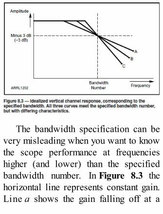
The bandwidth specification can bevery misleading when you want to knowthe scope performance at frequencieshigher (and lower) than the specifiedbandwidth number. In Figure 8.3 thehorizontal line represents constant gain.Line a shows the gain falling off at a

frequency much lower than thebandwidth frequency, but it has highergain than the others beyond thebandwidth frequency.

Line c is the other extreme. It showsthe gain falling off much closer to thebandwidth frequency, but shows lowergain past the bandwidth frequency. Youcan see that all three designs meet thebandwidth specification, but if you arelooking for performance beyond thebandwidth point, there can be bigdifferences among scope models. Inpractice the sloping line would not be asstraight as shown but rather a smoothcurve.

Frequency response (rise and fall

times). No, this is not an accidentalduplication of the frequency responseparagraphs above. If you are looking at adigital pulse — assuming it has perfectvertical rise and fall times — thebandwidth also limits how well the“perfect” pulse will be displayed. Thegenerally accepted formula — anapproximation — is

t(rise) = 0.35/bandwidth (in MHz)

Thus, as seen in Figure 8.4, a perfectsquare wave rise time will be seen as a35 ns rise time on a scope with a 10MHz bandwidth. Although “rise time”has been used in this explanation, thesame ideas and formulas hold for fall

times.Since perfect square waves, with

perfect rise and fall times do not exist, areal question is what exactly are youseeing? The answer is given by thisformula:

where t(rise) is the scope rise timenumber from the preceding paragraphand p(actual) is the actual pulse risetime.

If you want to visualize it, the answeris rather like the value of the hypotenuseof a right-angle triangle, where the scoperise time and the pulse rise time are the

two orthogonal sides.

Basic Capabilities of the HorizontalChannel

Horizontal sweep selection. Thiscontrol is usually marked in units of time(microseconds, milliseconds andseconds) As an example, selection 1 µstranslates into a sweep rate of 1 µs perhorizontal graticule marking. With theusual 1 mark per centimeter, it wouldtake 10 µs to sweep across the screen. A2 MHz sine wave (a complete periodequals 5 µs) would be seen as twocomplete sine waves across, assumingthe first one started at the left edge of thescreen.

Sweep magnifier. Many scopeshave a sweep magnifier control, either

5X or 10X. When selected, the sweeprate chosen is divided by this number —the magnifier expands the display by the5 or 10 factor.

Direct horizontal input. This is,perhaps, a rarely used feature (see thesection of Chapter 7 on Lissajousfigures). However, it does come inhandy from time to time. Unfortunatelythe sensitivity control for direct input(volts per cm) is often hidden —sometimes it is piggybacked on thehorizontal sweep setting control — butunmarked!

Accuracy and stability. Since thehorizontal sweep is used to measuretime or frequency, its accuracy and

stability are critical. Analog scopes,using purely analog circuits, usuallyhave much poorer specifications thandigital scopes. Not only do the analogcircuits making up the sweep have to bedesigned to be accurate, but they alsohave to be stable with temperature andtime. Digital scopes usually use acrystal-controlled clock and thus areless prone to circuit drift. While analogsweep circuits may require periodiccalibration, digital scopes rarely if everrequire this sort of alignment.

Delayed sweep. There are severalnames and techniques for displaying asection of a waveform that occurs laterthan the point where the horizontal

sweep is triggered. You can see suchterms as Delay Time Position, Holdoffa n d Segment Magnification. Thisfunction was described in an earlierchapter, but in summary these functionsallow you to pick the point you want toexamine and expand the sweep aroundthe selected point without changing thetrigger point. You would use this featureif, for example, your scope is set todisplay a 10 ms segment of waveformacross the screen, and you want toexamine closely a point on the waveformthat occurs 2 ms from the start of thesweep. You can examine any selectedpart of the entire 10 ms long waveformin a small selected area with a sweeprate of 1 µs/cm in this selected area.

Basic Capabilities of the TriggerSection

While many people focus on thebandwidth specification, the triggeringfeatures are of equal importance. If youdo not have a stable sweep, started by atrigger, you cannot see whatever youwant to look at. When it comes using anoscilloscope, setting the trigger is theone thing that gives many people aproblem. Not all of the selections listedfollowing will be found on every scope,but they are capabilities you shouldconsider.

Trigger sources . Channel A alone,Channel B alone, alternate channels A

and B , Line (60 HZ), external ( though atrigger input connector). The alternateselection triggers the sweep on channelA for the input on channel A, and then(alternately) triggers on channel B forthe input waveform on channel B.

Trigger modes and selections.There are generally at least two modes.AUTO triggers the sweep even if there isno discernible signal for triggering, butwhen a signal appears the mode changest o NORMAL. NORMAL allows you toselect manually the triggeringparameters: positive slope, negativeslope, selected positive voltage,selected negative voltage, zero volts,zero volt crossing and others.

Digital scopes have additional modessuch as single sweep, to be discussedlater. Older scopes, such as seen often atflea markets, may also have positionscorresponding to the “old” NTSC TVstandard waveform.

Digital ScopesThere are a number of specifications

that apply, some unexpectedly, to digitaloscilloscopes. As an example, look atFigure 8.5. The inputs of these scopesare set to sample the incoming waveformand then convert the measured value to adigital number. Simple in concept, but itcan cause problems such as in the figure.

A pulse is shown in A as it appears onan analog scope. B is the samewaveform, but sampled. If the samplingfrequency is not high enough, you willlose detail on the waveform even thoughthe specified bandwidth is high enoughfor the waveform.

How high should the samplingfrequency be? There is no standardanswer. Certainly five times the highestfrequency you want to see is not enough.Ten times? A hundred times? That mightbe enough, but remember that you arelooking at the highest frequency youwant to see, so for rectangular pulsesyou need to see harmonics.

A good compromise would use the

bandwidth as the base number, and thenperhaps a high multiple (500? 1000?) ofthe bandwidth would be enough. If youbelieve these paragraphs have avoidedan exact answer, you are correct. Somemanufacturers use data prediction andsmoothing techniques to at least fill inthe gaps artificially, if not reallyimprove the response to very fasttransitions.

Another technique used by somedigital oscilloscope designers moves thehorizontal trigger on successive sweeps(Figure 8.6). If the waveform you wantto see is absolutely repetitive, with littleor no jitter, one sweep is made in thenormal fashion started by the sweeptrigger. A second sweep is made,

delayed by perhaps 1/10 of the samplerate in time. A third sweep is made,delayed by twice this increment, and soon. At the end of 10 sweeps, 10 sampleshave been taken in place of the one thatthe usual sampling would haveproduced. Thus the waveform issampled at 10 times the normal samplerate, but it required 10 sweeps to do so.Again the waveform must be absolutelyrepetitive and virtually jitter-free for thistechnique to work, but when it does it isvery effective.

This just one of the more interestingand complex problems that occur whenusing a digital scope. Certainly theyhave advantages, but an understanding of

the functions is very necessary to be ableto understand what you are measuring.

Number of bits of the input A/Dconverter. Again we have a simple ideathat gets complicated very quickly.Suppose the A/D converter has 12 bits.This means the input voltage can bedivided into 21 2 parts, or 4096 parts.However system noise and uncertaintywill knock out one or more bits. Butobviously, better to opt for more, even ifseveral are not effective.

Memory size. Ready to do somemultiplications? Try this: The memoryneeded is equal to (the number of bits ofa single point on the waveform) times(the number of samples per second)

times (the amount of waveform you wantto see in seconds or fractions of asecond). Now consider that there aretwo channels — do you want to doublethe memory size or cut the number ofsamples per second in half, giving halfto each channel?

Processor capability. Okay, nowthe data is in memory. Can the processorhandle it? Certainly, if you have a self-contained digital scope, the designersmade sure there is enough horsepower toprocess this data and generate thedisplay you want. But remember, someof the processor capability is going tocomputer bookkeeping, backgroundoperations and display generation.

With a self-contained oscilloscope,such as the one in Figure 8.7, themanufacturer has sized the memory andprocessor to match the specifications.The controls on the right side are actualmenu selectors, and the current settingsare shown on the right side of the screen.

Now if you are using an outboardscope that plugs into the USB port, isthere a bottleneck? Is the hardwarecapable or the operating system fastenough? Were you planning to plug intoan old, slow computer? Figure 8.8 isfrom a scope that plugs into an iPad oriPhone. Its bandwidth is 5 MHz, andwhile it has a good set of functions andcontrols, its host devices do not have

much memory or computing horsepower.Things do indeed get interesting, and notall the questions have discrete answers.

Processor type. Until now therehas been an assumption that the externaldigital scope plugs into a Windowscomputer. Is the unit you are planning tobuy available with software compatiblewith non-Windows operating systems?How about Apple or Linuxcompatibility?

Convenience. Many new scopesoffer convenient features, such asautomatic setup. Connect a waveform,and the scope sets the vertical voltagescale, horizontal sweep rate and trigger

settings to numbers it measures asapplicable. Then you can tweak thesesetting any way want. How about one-button measurements? Select from amenu to get readout of peak-to-peakvoltage, maximum voltages, averagevoltage, frequency, periods and othermeasurements. Is there a cost? Ofcourse, but if you are making repetitivemeasurements it might well be worth it.

Waveform storage . In an earlierchapter it was noted that digital scopesstore the input data, and thus can providea stored picture. One number that can bespecified is how big this picture can be;that is how many seconds ormilliseconds of data can be stored.

Time scale. Does the scope offerboth linear sweep and logarithmicsweep? A log sweep can be invaluablewhen looking at a long sequence ofevents.

Direct multichannel digitalinputs. As described earlier in thisbook, some scopes offer multichannel (atleast four) inputs for looking at fourdigital signals simultaneously. Usuallythe allowable voltage range for theseinputs is less than allowed for analogchannels A and B, but sufficient fornormal digital signals.

Anything else? Is there any end to thislist? Of course not. When anoscilloscope is based on a digital

processor, anything that can be imaginedas a function for a digital processor canbe programmed. There is a cost, but aswas noted in the first paragraph of thischapter. Your first task is to decide whatyou want to do with the scope.

Other Features and Types

LimitationsAs discussed in Chapter 7, some

advanced digital scopes include testinstruments, taking advantage of thememory and processor used in the basicoscilloscope. Usually, each of thesefeatures are specified in some detail. As

an example, where an FFT (Fast FourierProcessor) is included, the number ofpoints and speed are also specified.There are, however, several cautions tobe noted. First, if the A/D and analogfront end are limits on the scopebandwidth, the included other functionswill be limited to these bandwidths.Don’t expect a 30 MHz bandwidth scopeto show signal spectrum to 500 MHz!

Next, while digital processors andtheir associated memory are verycapable of being programmed as signalfunction generators, many of thesecapabilities and others cannot be usedsimultaneously with the oscilloscopefunctions. Thus if there is a signal

generator that you plan to use to test acircuit, selecting the signal generatorfunction may disable the scope function.

Interfaces, Connections, and AdditionsNot listed in Chapter 7, but of some

importance, is the ability of some scopesto be connected to analysis or simulationprograms such as MATLAB, or to otherhardware — perhaps a large capacityrecorder. Since these functions and thegeneral complexity of some modernoscilloscopes can be rather high, youmight look for detailed user instructionsand video demonstrations on the CD orDVD that comes with the scope. Usuallythe CD contains the user manual and

other information.

Just One More Type of OscilloscopeAvailable for download, often free

and very interesting, is the set ofhardware-free oscilloscopes. These usea personal computer sound card as thechannel connections. The software,similar to that used with hardwarescopes that connect to a PC via a USBconnection, is hosted on the PC.

There are, of course, cautions andlimitations associated with thisapproach. Since the sound card isinterfaced with (sometimes) unknownsignals, protection for your sound card isstrongly suggested. A protection circuitfor this situation is given in Chapter 7.

Figure 8.9 is a screen shot from onesuch scope. Downloading and setting itup takes only a few minutes. However,the bandwidth, in this case, is limited tothe capability of your sound card.Generally, for sine waves, this means alower frequency limit of perhaps 20 Hzand an upper frequency limit of 20 kHz.

For pulses and other non-sinusoidalsignals where Fourier analysis predictsfrequency content of multiples of thebase waveshape, the best you can obtainwithout serious distortion is perhaps 20kHz divided by 5, so that the 5thharmonic energy will be passed and thedisplayed waveform recognizable. Sincethe source of these scopes is the Internet,

and names, addresses and cost (if any)are constantly changing it will probablytake you as much time to find one ofthese software scopes on line as it willto download it and get it working!

Appendix 1

SoftwareOscilloscopes —Capable and Free!

Over the years, I have seen and useda wide variety of oscilloscopes in myhome workshop. They all had one thingin common — a cost.

As discussed in earlier chapters,there are still quite a few old-line analog

oscilloscopes for sale — self-containedwith a large CRT facing out of the frontpanel. The newer generations of scopesare digitally based, where after somesmall analog input circuits the signalgoes into one or two analog-to-digital(A/D) converters. From this point on thesignals you want to see are in acomputer of sorts built into the scope. Infact some modern scopes don’t includethis computation ability but connect toyour personal computer.

More recent is a new set ofoscilloscopes that are tiny enough to fitin your shirt pocket. Digilent makes aunit that interfaces though a USB port toa PC. Another unit made by Oscium

connects to an iPhone, iPod or iPad (seeAppendix 3). Unfortunately these ultra-miniature scopes have a limitedfrequency bandwidth.

Another option is a scope requiringno hardware! Since today’s scopes areprimarily software, running in some sortof computer, is seems that all you needis a front end consisting of an A/Dconverter. You already have A/Dconverters built into your PC — thesound card. Why not use that?

This is exactly what others realized,and there are probably a dozen, orperhaps even more, software-onlyscopes available for download on theInternet. Many of them are free for ham

use. As with any download program, anactive virus or malware checker is anabsolute necessity before running such aprogram.

What’s The Catch?There are really two major

limitations to using a software-onlyscope. The first is that that the signal tobe seen is connected directly to thesound card. If this signal voltage is toohigh — poof goes the sound card (oreven worse, the sound card circuitry onthe mother board!). Therefore a simpleprotection circuit, such as the onedescribed in Chapter 7, is needed to

protect the sound card. Be sure to takethe time to build an adequate protectioncircuit!

The second limitation is frequency.You can generally get reasonable resultson sine waves up to the sound card limitof 20 kHz or so, but as the figures in thisAppendix show, non-sinusoidalwaveforms can be badly distorted astheir repetition frequency goes up.

What Do You Get Free?As noted before, there are many

software scopes available. SoundcardOscilloscope, V1.41 by ChristianZeitnitz (www.zeitnitz.eu/scope_en)

was used here to show the features andlimitations typical of these scopes. Makeno mistake, this is a full featured, stableand in fact fun-to-use test instrumentwithin its limitations (primarilyfrequency limitations).

The tests and resulting pictures herewere made using both a three-year-oldPentium PC running Windows 7 and afive-year-old Asus Netbook, runningWindows XP. There was no noticeableperformance difference with eithercomputer.

Soundcard Oscilloscope comes witha 16-page manual in PDF format andbuilt-in help files. As usual withsoftware documentation and help files,many questions go unanswered, but alittle experimentation often answers thequestion.

The scope output plugs into the LINEINPUT jack of the soundcard. Becausethe scope is dual channel, a dual channel

(or stereo) input is needed. On most PCsthe microphone input is monaural andwill not be suitable.

When you bring up the software, afterthe licensing notice, a set of tabs on topare used to select what you want to do.Figure A1.1 shows the SETTINGS tab.As you can see the input selected for thePC is LINE IN. Next you can go to theOSCILLOSCOPE tab and make therequired time base and voltage settings.Then back to the SETTINGS tab and saveyour settings for future use. Also checkthat the sound card settings in your PChave the gain for LINE IN turned up.

Figure A1.2 shows the screen whent h e OSCILLOSCOPE tab has beenselected. Voltage calibration is notexact; the voltage scale is arbitrary andits range is a 16-bit number. However ifyou put a known waveform in one

channel, you can get reasonablemeasurements by adjusting the cursorand comparing the unknown waveformwith the known waveform. The relativeaccuracy is one part in 32,768. Betweenthe amplitude controls and the resistorsin the sound card protection circuit, youhave to work a bit to adjust the system toshow your waveform.

The horizontal sweep rate iscalibrated in total range, presumablyacross the entire screen — not time percm as in most scopes. Slightly confusingis the 1 CHANNEL mode (second column,near the bottom). 1 CHANNEL does notmean single channel; it means twoseparate channels as contrasted to the

other available settings of adding andsubtracting the two channels.

Figure A1.2 shows a roughly 2 kHzsquare wave and the same frequencytriangular wave on the scope face.Notice that the square wave is relativelysquare — compare this to Figure A1.3where a 10 kHz square wave is shown.

Mathematically, by a techniqueknown as Fourier analysis, a squarewave can be shown to be made up of thesum of a sine wave at the fundamentalfrequency added to other sine waves atthe third harmonic, fifth harmonic,seventh harmonic and so on — in otherwords all odd harmonics. Eachharmonic has a specific amplitude. This

is discussed in Chapter 4 and Chapter 7of this book. The result is a display of avery distorted square wave when theseharmonics fall outside the sound card’s20 kHz bandwidth. At least one softwarescope claims performance related to thesound card sampling rate — perhaps upto 96 kHz or more.

Figure A1.4 shows the display whenthe FREQUENCY tab is selected. This isactually a spectrum analyzer. Here a 1kHz square wave shows the expectedharmonics at 3 kHz, 5 kHz, 7 kHz and soon. Unfortunately, the amplitudes here

are not shown accurately.The SIGNAL GENERATOR tab, Figure

A1.5 provides a set of selected outputwaveforms, just as with expensive self-contained scopes. Another includedcapability is an audio recorder in theEXTRAS tab (Figure A1.6), which youcould use to record the waveform underexamination. Finally, the XY GRAPH taballows you to see Lissajous figures,which could be very handy in comparingrelated audio frequencies.

Other Free Software ScopesMany of the other available software

scopes are quite similar to the one justdescribed. A short Internet search willbring up both scope downloads andmore information about these devices. Afew versions include on-screenmultipurpose voltmeters, frequencymeters, ohmmeters, ammeters, and alarge variety of other test equipment.Some require some external circuitry. Afew use special sampling techniques thatthey claim allow use beyond thecapability of the sound card — althoughprobably only for a limited section of awaveform.

To see a fraction of what is available

set your search engine to find the exactphrase “software oscilloscope” and thewords “free” and “download.”Whatever the true capabilities of thesescopes are the price is right. All youhave to do is spend your time exploringthese very useful programs.

Appendix 2

QST ProductReview: RigolDS1052E andTektronixTBS1042Oscilloscopes

This review, by Phil Salas, AD5X,originally appeared in October 2013QST.

Most hams have basic test equipmentconsisting of at least a digitalmultimeter, SWR meter and dummyload. These three instruments providethe ability to do basic troubleshooting.Additional equipment often includes anaccurate RF power meter, a frequencycounter and an oscilloscope. Of these,historically the oscilloscope has beenthe most expensive, leading hams toexplore the surplus equipment market.Used analog oscilloscopes can be quitegood, but they are also large andinconvenient for recording data. If

something goes wrong, they may bedifficult and expensive to repair.

Digital sampling oscilloscopes(DSOs) have become available at pricesjustifiable for many ham experimenters.The two reviewed here provide featuresand capabilities that will satisfy mosthome users.

The Oscilloscope DecisionProcess

In the past, factors to be consideredwhen choosing an oscilloscope includedthe number of simultaneous signals thatyou might need to measure, thebandwidth necessary, on-screen digital

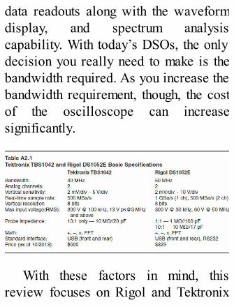
data readouts along with the waveformdisplay, and spectrum analysiscapability. With today’s DSOs, the onlydecision you really need to make is thebandwidth required. As you increase thebandwidth requirement, though, the costof the oscilloscope can increasesignificantly.

With these factors in mind, thisreview focuses on Rigol and Tektronix

DSOs with a 40 to 50 MHz bandwidth,as this is sufficient to permit mostmeasurements desired at the lowest cost.As you can see in Table A2.1, these twoinstruments have very similar basicspecifications. Detailed specificationscan be found on the manufacturers’websites.

Let’s Make a Few TestsTo see how the oscilloscopes

perform, I selected several tests that Ithought hams would find useful andinteresting. For the first test, I looked atthe measured frequency response of theoscilloscopes. I measured RF power

with a calibrated setup and then checkedthe amplitude of the frequency on 7, 28and 50 MHz. The Rigol has a 50 MHzbandwidth and the Tektronix has a 40MHz bandwidth, so I would expect tosee some rolloff on 10 and 6 meters.This doesn’t mean you can’t look atsignals, just that the amplitude of higherfrequency signals may not be completelyaccurate.

My next test involved measuringtransmitter overshoot. When atransceiver’s output power is reduced,often the transceiver output willovershoot (be higher than) the set poweron the first CW character or speechsyllable. This happens because a finite

time is required for the transceiver’sALC to control the signal. If overshoot ishigh enough, it can trip protectioncircuitry in an external RF poweramplifier or even damage it. For this testI set my Icom IC-706MKIIG transceiverto 25 W output, as this is theapproximate drive power needed for fulloutput from my Elecraft KPA500amplifier.

Next I wanted to look at the amplifierenable/disable timing versus the RFsignal output. This timing is importantwhen driving an amplifier to ensure thatno hot switching of the amplifier ortransceiver takes place. (Hot switchingmeans transmitting a signal before relay

contacts have closed.) The amp key-to-RF signal and RF signal-to-amp unkeytimings are both important because youwant to make sure that there is no chanceof hot switching on either amplifierkeying or amplifier unkeying. I fed theIC-706MKIIG transceiver’s HSENDoutput to channel 2 on the oscilloscopeand set the oscilloscope to trigger onchannel 2. A falling edge trigger showsthe amp-enable timing, and a rising edgetrigger shows the amp-disable timing. Icould have fed HSEND into theEXTERNAL TRIGGER input on theoscilloscope, but I wanted to displayHSEND along with the RF signal to betterclarify the timing.

My final test involved two-tonetesting of my transceiver. A two-tonetest is a standard test of a transceiver’slinearity that normally requires aspectrum analyzer. However, bothoscilloscopes have a fast Fouriertransform (FFT) math feature that shouldpermit display of signals in thefrequency domain. For this test, a two-tone audio signal is fed into thetransceiver’s microphone input, and thecomposite level adjusted for 25 W peakoutput. After displaying the normalmodulated RF signal on theoscilloscope, select the FFT mode andmake sure you are displaying in the dBscale. Use the vertical knob to select

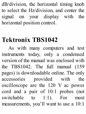
dB/division, the horizontal timing knobto select the Hz/division, and center thesignal on your display with thehorizontal position control.

Tektronix TBS1042As with many computers and test

instruments today, only a condensedversion of the manual was enclosed withthe TBS1042. The full manual (159pages) is downloadable online. The onlyaccessories provided with theoscilloscope are the 120 V ac powercord and a pair of 10:1 probes (notswitchable to 1:1). For mostmeasurements, you’ll want to use a 10:1

probe because the capacitive loading ofa 1:1 probe will be a problem for higherfrequency RF signals. Also, a 10:1probe provides better overloadprotection should you accidentallyconnect to a high voltage source. A 1:1probe is most usable for audiomeasurements at very low signal levels.

An important feature of anyinstrument is its ease of use. Therefore Iattempted to use the TBS1042 withoutreading the manual, other than readingabout how to compensate the probes. Asit turned out, I was able to quickly set upand measure everything in all the testswithout cracking the book! What makesthis easy is the AUTOSET button that sets

up the unit for you. Just apply a signaland press AUTOSET. Within a fewseconds you’ll have a display that willbe very close to what you want. Fromthis point, you can simply change thevertical sensitivity and horizontal timingto refine the display to your liking.

The USB port on the front of the unitprovides either print or save functions.The TBS1042 determines if theconnected device is a printer or memorystick, and will either print or save thescreen data when the PRINT button ispushed.

The frequency response test resulted

in a measured rolloff of 0.57 dB on 10meters, and 1.67 dB on 6 meters, muchbetter than the manufacturer’s 3 dBspecification for the 40 MHz bandwidth.

For the overshoot test, I set mytransceiver output to a nominal 25 Woutput level and triggered the TBS1042on the channel 1 input. You have achoice of enabling either two horizontalcursors to measure amplitude, or twovertical cursors to measure time. Ienabled the horizontal cursors to displaythe overshoot amplitude. The results areshown in Figure A2.1. Note that with aset output power of 25 W, the outputpeaks at 72 V peak (100 W) on the firstdit

Next I looked at the amp-key enable(Figure A2.2) timing with thetransceiver set for full break-in. Thebottom trace is the amp-enable HSENDline from the radio. The results areinteresting. The amp-enable-to-RFoutput time of 15 ms is fine for vacuumrelays and PIN diodes. It is probablyokay for open frame relays used on manyamps not designed for full break-in(QSK) operation, but it is marginal. Atypical enable time for open-framerelays is 12-20 ms.

The amp disable timing (FigureA2.3) shows a problem with QSK-switched amplifiers. The amp disableline goes high about 4 ms before RFdrops to zero (the vertical cursors wereenabled to better show this). So you mayhot switch an amplifier that is operating

in QSK. To be on the safe side, IC-706MKIIG users should only operatesemi break-in.

My last test was a two-tone test ofthe transceiver output. Figures A2.4 andA2.5 compare the display of a spectrumanalyzer (a Rigol DSA815-TG) with the

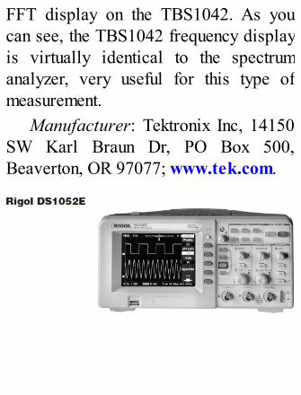
FFT display on the TBS1042. As youcan see, the TBS1042 frequency displayis virtually identical to the spectrumanalyzer, very useful for this type ofmeasurement.

Manufacturer: Tektronix Inc, 14150SW Karl Braun Dr, PO Box 500,Beaverton, OR 97077; www.tek.com.

The DS1052 did not includeabbreviated instructions, but the fullmanual (166 pages) is downloadableonline. The DS1052E includes a 120 Vac line cord, a pair of switchable10:1/1:1 oscilloscope probes, and aUSB cable for interfacing to yourcomputer.

Again, I attempted to use the

oscilloscope without reading the manual,other than the section on probecompensation. And again I had noproblems. The AUTO button on the Rigoloscilloscope is equivalent to theAUTOSET button on the Tektronixoscilloscope. After applying a signal,press AUTO and then adjust the verticalsensitivity and horizontal timing to refinethe display to your liking.

The only thing I had problems withwas saving the display to a USB memorystick. The SAVE procedure is veryflexible, permitting you to save differentformats and even permitting you to namethe files. The SAVE process wasn’tintuitive, requiring me to refer to themanual.

The frequency response test wasinteresting. The specification is for a 3dB rolloff at 50 MHz, but I found norolloff at all on 6 meters.

For the overshoot and amp-key/unkeytiming tests, I found I could displayeverything at the same time. When I wentto the TRIGGER menu I found that one ofthe options was triggering on both

negative and positive going slopes of thetriggering signal. This let me look at theamp-key HSEND going low on transmitand high on un-key, and the resultant RFsignal — including overshoot. Theresulting timing waveform is shown inFigure A2.6. The bottom trace is theamp-enable/disable (HSEND) line out ofthe IC-706MKIIG.

I also tested the overshoot and amp-disable timing separately so as toprovide detail similar with the TektronixTBS1042 tests. I enabled the verticalcursors in both cases so as to moreeasily display the time. From thedetailed view, I found that the first-ditovershoot lasts less than 2 ms (Figure

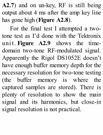
A2.7) and on un-key, RF is still beingoutput about 4 ms after the amp key linehas gone high (Figure A2.8).

For the final test I attempted a two-tone test as I’d done with the Tektronixuni t . Figure A2.9 shows the time-domain two-tone RF-modulated signal.Apparently the Rigol DS1052E doesn’thave enough buffer memory depth for thenecessary resolution for two-tone testing(the buffer memory is where thecaptured samples are stored). There isplenty of resolution to show the mainsignal and its harmonics, but close-insignal resolution is not practical.

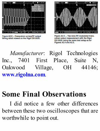
Manufacturer: Rigol TechnologiesInc., 7401 First Place, Suite N,Oakwood Village, OH 44146;www.rigolna.com.

Some Final ObservationsI did notice a few other differences

between these two oscilloscopes that areworthwhile to point out.

Both oscilloscopes have a 5.7 inchdiagonal color display. However, youcan turn off the right-side menu on theRigol, which provides a little moredisplay area than on the Tektronix. TheTektronix oscilloscope takes about 30seconds to boot up, whereas the Rigol isup and running in less than 10 seconds.Also, the Tektronix takes about 30seconds to save a file to a USB memorystick, whereas the Rigol takes about 1second. And I did like the Rigol’s abilityto trigger on both a positive and negativetrigger on the same display. However,the Tektronix oscilloscope’s ability todisplay a frequency domain two-tonetest spectrum is important to me.

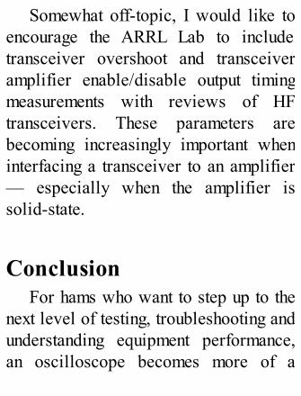
Somewhat off-topic, I would like toencourage the ARRL Lab to includetransceiver overshoot and transceiveramplifier enable/disable output timingmeasurements with reviews of HFtransceivers. These parameters arebecoming increasingly important wheninterfacing a transceiver to an amplifier— especially when the amplifier issolid-state.

ConclusionFor hams who want to step up to the

next level of testing, troubleshooting andunderstanding equipment performance,an oscilloscope becomes more of a

necessity. Fortunately, digital samplingoscilloscopes have become surprisinglyaffordable. The two oscilloscopesdiscussed here will provide most of thecapabilities desired by the moresophisticated ham at a price that iseasily justifiable.

Appendix 3

QST ProductReview: OsciumiMSO-204PortableOscilloscope

This review, by Paul Danzer, N1II,originally appeared in June 2014 QST.

Some years ago (OK, many yearsago) I was a young engineer, assigned toconduct tests on a US Navy ship used toevaluate various electronic devices.When I drove up to the pier late oneSunday evening, the men on duty at thegang plank had an order to allow meonto the ship, but there was no one elsearound to help me. The test wassupposed to start early Monday morningand I had a 70+ pound Tektronixoscilloscope that had to be carried upthree flights of stairs to the test room.The navy calls the stairs ladders; Icalled them torture — 70+ pounds,three flights of stairs!

I had forgotten about this incidentuntil the Oscium iMSO-204 portableoscilloscope was delivered to my door.And portable it is! It’s shirt pocket size,and the weight is obviously not aproblem — the problem is to not lose itin your pocket.

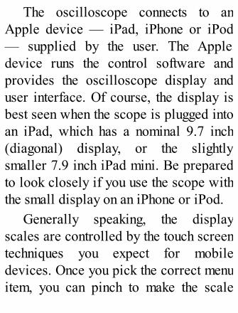
The oscilloscope connects to anApple device — iPad, iPhone or iPod— supplied by the user. The Appledevice runs the control software andprovides the oscilloscope display anduser interface. Of course, the display isbest seen when the scope is plugged intoan iPad, which has a nominal 9.7 inch(diagonal) display, or the slightlysmaller 7.9 inch iPad mini. Be preparedto look closely if you use the scope withthe small display on an iPhone or iPod.

Generally speaking, the displayscales are controlled by the touch screentechniques you expect for mobiledevices. Once you pick the correct menuitem, you can pinch to make the scale

smaller or slide your finger wider tomake it bigger. Given a list, slide yourfinger up or down from the currentsetting to the new setting.

There are two Oscium oscilloscopemodels available. This review featuresthe iMSO-204, which has two analogand four digital channel inputs. The lesscapable (and less expensive) iMSO-104has a single analog channel anddifferences in the detailedspecifications.

Given its size, can the iMSO-204really replace a scope with a built-in 6inch display and a front panel full ofknobs? Will it really replace a largercomputer-controlled unit that requires a

PC or laptop to work?

Why is It So Small?The answer, of course, is that with

the increasing speed and accuracy ofanalog-to-digital (A/D) converters, lessanalog circuitry is needed up front.Other than some signal switching,selection of ac or dc coupling andperhaps some protection circuitry, youcould go directly into an A/D converterand send the output to an external digitalprocessor. Voltage scaling, triggering,level shifting and formatting for displayis all done in software.

This is particularly true for digital

inputs, where the A/D converters are notneeded. Oscium specifies the digitalinputs for –0.5 to +7 V. Depending onthe probe settings (×1 or ×10), theanalog inputs are limited to –8 to +13 Vor –40 to +40 V — certainly sufficientfor today’s solid state circuits.

Getting StartedFirst you have to download the

software (free, of course) from theApple store (go towww.oscium.com/oscilloscopes/imso-204 and click the download button onthis page).

Next, connect the probes. The probes

for the two analog input channels slidein, no problem. To use the four digitalchannel inputs, the digital connectors —four wires plus a ground — have to beplugged into a set of probes. Lookcarefully. The mating pins on the probesare at an angle — the wire sleeves slidein at that angle to connect. A magnifyingglass might help! These connections arefriction fits, so a hard pull maydisconnect a probe from its connectingwire.

To fire up the scope, turn off yourApple device (from now on I am justgoing to refer to the device as an iPad).Then plug the scope into the iPadconnector. In the last year or so Apple

has changed connectors. The scope hasan older 30 pin connector, but Osciumoffers an optional adapter to connect thescope to devices with the newerLightning connector.

Finally, turn on your iPad, select theOSCIUM icon, and you are set. Perhapsthe first thing you will want to do isexplore the functions. By touching theicon in the lower right corner the scopegoes into a demo mode, where most, butnot all functions are available.

Analog and Digital ScopeFunctions

The scope comes equipped with two

conventional analog probes and twoanalog channels. The trigger icon at thebottom allows you to select thetriggering source and mode. Figure A3.1shows the waveforms from two analogsignals.

Somewhat unusual are the four digitalchannels. They do not use an A/Dconverter — the probes connect directlyto digital circuitry in the scope. Whenworking with digital circuits, often you

would like to look at more than twosignals at a time. Figure A3.2 shows thewaveforms from four stages of a 4790digital counter chip, wired as a divide-by-10 circuit (traces D1 to D4 at thebottom of the screen). Much to mysurprise — although not captured in thescreen shot — one of the stages showed“snivits” — short, narrow spikes due toslight mistiming built into the circuit.Since the snivits were on anintermediate stage, they did not affect thedivide-by-10 feature.

A Good, Clear PictureWith older analog scopes, to get a

good, clear picture you have to carefullyadjust intensity (or brightness), focus,and triggering. With the iMSO-204, thefirst two are no longer a considerationbecause the display is synthesized in thedigital realm. Triggering is still acritical factor. This scope does not havean external trigger input, but does offer awide variety of trigger capabilities fromthe selected inputs.

When using the digital inputs, any ofthe four can be selected as the trigger.This is a very handy feature whenlooking at series circuits such ascounters.

The two analog inputs, A and B, maybe combined or selected in various ways— either, alternate, or both as well aspositive, negative, dc level, up slopeand down slope — in other words a full

assortment of trigger capabilities. Bytouching the TRIGGER icon on the bottomof the screen, the trigger selection menui n Figure A3.3 comes up and you canselect the actual trigger level. Yourselection immediately goes into effectafter you next touch a blank area of thescreen and your waveform then becomesvisible.

The DisplayAt the risk of upsetting touchscreen

lovers, remember that the screen onmany devices can be more sensitive thanyou expect. Some settings require morethan one tap or a combination of taps and

swipes. On occasion, the device willbring up menus and functions you did notexpect. Oscium has designed theirsoftware so that if you touch anunoccupied portion of the screen, usuallythe software will revert to the previousstate or display.

The scope technology used is one ofsampling the inputs and digitally storingthe result, so onscreen storage in a built-in function. In the lower right corner ofFigure A3.4 is a PLAY icon that setseither normal scope displays or a stop-stored display. You can look at an eventeither with a manual freeze or anautomatically triggered freeze — veryhandy when chasing transients.

The Oscium software offers twofunctions for capturing and savingoscilloscope screen shots. One capturesthe screen so it can be e-mailed (I didn’ttry this). The other stores a screen shotto the iPad photo storage, but the manualsuggests you use the iPad’s built-inpicture store function, which is how thescreen shots in this review were stored.The iPad’s screen capture functionrequires pressing two buttons, and Ifound it “touchy,” sometimes requiring acouple of tries. Just blame it on theoperator!

Built-In Spectrum AnalyzerMany, if not most, of today’s digital

oscilloscopes include both an FFT (fastFourier transform) analysis/display

function and a signal/function generator.This scope does not include a generator,but does offer FFT, integration anddifferentiation. Admittedly it is not clearjust how applicable the integration anddifferentiation functions are to most hamprojects, but if you have them, you willprobably find a use for them.

There is also a set of 15 very handyautomatic measurement routines. Theseinclude, to quote from the manual:Minimum, Maximum, Mean, Peak toPeak, RMS, Duty Cycle (+), Duty Cycle(–), Pulse Width (+), Pulse Width (–),Cycle Mean, Cycle RMS, Frequency,Period, Rise Time, and Fall Time.Selecting these functions is quite simple,

but understanding exactly what you aremeasuring takes a bit of practice.

Is It Capable Enough?The answer to this question depends,

of course, on what you want to do theiMSO-204. The bandwidth is specifiedas 5 MHz, but you can easily see sinewaves — RF — to 14 MHz and beyondwithout known amplitude calibration.However, it is a sampling scope. Thehigher the frequency, the fewer thesamples per sine wave, so perhaps thewaveform shown at higher frequenciesis less representative of the actualsignal. In Figure A3.4 you can see the

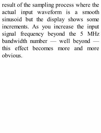
result of the sampling process where theactual input waveform is a smoothsinusoid but the display shows someincrements. As you increase the inputsignal frequency beyond the 5 MHzbandwidth number — well beyond —this effect becomes more and moreobvious.

Figure A3.5 is a screen capture of a7.15 MHz SSB signal, taken at lowpower at a dummy load. This is past therated 5 MHz bandwidth, and the scopewas triggered to show syllables. Similar

results were seen at 14 MHz, but ofcourse the vertical calibration does nothold past the rated bandwidth.

One important factor — keep theinput waveform amplitude down withinthe specified limits. Even if you do notdamage anything, the waveform will bedistorted if the input A/D is near itsamplitude limit.

In SummaryIf you need something very portable

— for example on ARRL Field Day orwhen going to a restricted space to trackdown a transient on the local repeater —and you already own an iPad or similar

device — this might be a good choice.The 5 MHz bandwidth is certainly alimitation, but it does show higher inputsignal frequencies.

Some skill and practice is needed toconquer a multifunction iPad with theOscium software. It’s not as simple as,say, selecting a photo to view. As withmost complex equipment, the instructionbook does not cover everything. Somefeatures are self-explanatory as seen onthe screen; others not in the book requiretrial and exploration.

There are similar products, and atleast one about the same size and withsame bandwidth. However they requirea laptop (or PC) and thus are not as

portable and convenient.As a replacement for your normal

bench oscilloscope, this is probably notthe best choice. But for its uniquecharacteristics — size and portability —it works, and well enough to include inyour proverbial portable tool box.

To get a better idea of how theiMSO-204 works, you can download themanual from the Oscium website and thesoftware from the Apple store. Themanual explains how to turn on and usethe demo mode without having the scopehardware.

Manufacturer: Oscium, A DechniaLLC, 5909 NW Expressway, Suite 269,Oklahoma City, OK 73132;

www.oscium.com.