Copyright © Cengage Learning. All rights reserved.

Functions

Copyright © Cengage Learning. All rights reserved.

2.2 Graphs Of Functions

3

Objectives

► Graphing Functions by Plotting Points

► Graphing Functions with a Graphing Calculator

► Graphing Piecewise Defined Functions

► The Vertical Line Test

► Equations That Define Functions

4

Graphs Of Functions

The most important way to visualize a function is through its graph.

In this section we investigate in more detail the concept of graphing functions.

5

Graphing Functions by Plotting Points

6

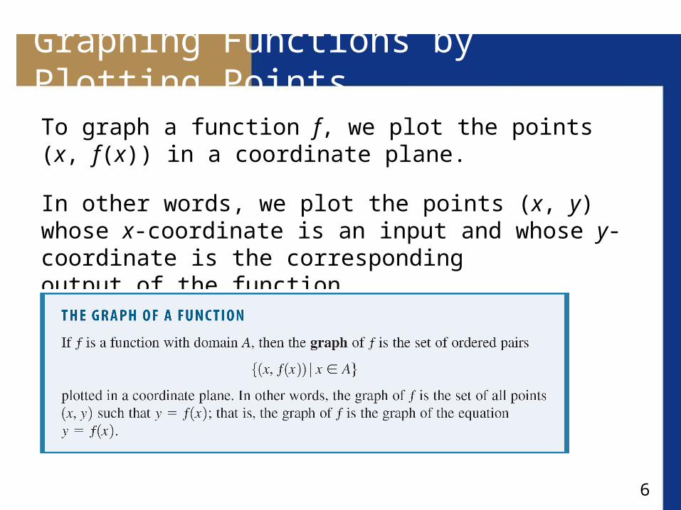
Graphing Functions by Plotting Points

To graph a function f, we plot the points (x, f (x)) in a coordinate plane.

In other words, we plot the points (x, y) whose x-coordinate is an input and whose y-coordinate is the correspondingoutput of the function.

7

Graphing Functions by Plotting Points

A function f of the form f (x) = mx + b is called a linear function because its graph is the graph of the equation y = mx + b, which represents a line with slope m andy-intercept b.

A special case of a linear function occurs when the slope is m = 0.

The function f (x) = b, where b is a given number, is called a constant function because all its values are the same number, namely, b. Its graph is the horizontal line y = b.

8

Graphing Functions by Plotting Points

Figure 2 shows the graphs of the constant function f (x) = 3 and the linear function f (x) = 2x + 1.

The linear function f (x) = 2x + 1The constant function f (x) = 3

Figure 2

9

Example 1 – Graphing Functions by Plotting Points

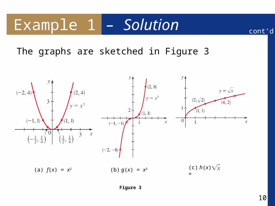
Sketch graphs of the following functions.

(a) f (x) = x2 (b) g (x) = x3 (c) h (x) =

Solution:We first make a table of values. Then we plot the pointsgiven by the table and join them by a smooth curve to obtain the graph.

10

Example 1 – Solution

The graphs are sketched in Figure 3

(b) g(x) = x3(a) f(x) = x2 (c) h(x) =

Figure 3

cont’d

11

Graphing Functions with a Graphing Calculator

12

Graphing Functions with a Graphing Calculator

A convenient way to graph a function is to use a graphing calculator.

13

Example 2 – Graphing a Function with a Graphing Calculator

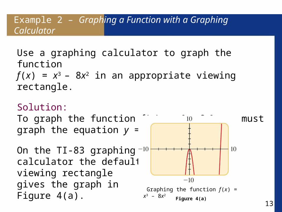
Use a graphing calculator to graph the function f (x) = x3 – 8x2 in an appropriate viewing rectangle.

Solution:To graph the function f (x) = x3 – 8x2, we must graph the equation y = x3 – 8x2.

On the TI-83 graphingcalculator the default viewing rectangle gives the graph in Figure 4(a).

Graphing the function f (x) = x3 – 8x2

Figure 4(a)

14

Example 2 – Solution

But this graph appears to spill over the top and bottom of the screen.

We need to expand the vertical axis to get a betterrepresentation of the graph.

The viewing rectangle [–4, 10] by [–100, 100] gives a more complete picture of the graph, as shown in Figure 4(b).

cont’d

Graphing the function f (x) = x3 – 8x2 Figure 4(b)

15

Graphing Piecewise Defined Functions

16

Graphing Piecewise Defined Functions

A piecewise defined function is defined by different formulas on different parts of its domain.

As you might expect, the graph of such a function consists of separate pieces.

17

Example 4 – Graphing Piecewise Defined Functions

Sketch graphs of the functions.

18

Example 4 – Solution

If x 1, then f (x) = x2, so the part of the graph to the left of x = 1 coincides with the graph of y = x2, which we sketched in Figure 3.

(b) g(x) = x3(a) f(x) = x2 (c) h(x) =

Figure 3

19

Example 4 – Solution

If x > 1, then f (x) = 2x + 1, so the part of the graph to the right of x = 1 coincides with the line y = 2x + 1, which wegraphed in Figure 2.

cont’d

The linear function f(x) = 2x + 1The constant function f(x) = 3

Figure 2

20

Example 4 – Solution

This enables us to sketch the graph in Figure 6.

The solid dot at (1, 1) indicates that this point is included in the graph; the open dot at (1, 3) indicates that this point is excluded from the graph.

cont’d

Figure 6

21

Graphing Piecewise Defined Functions

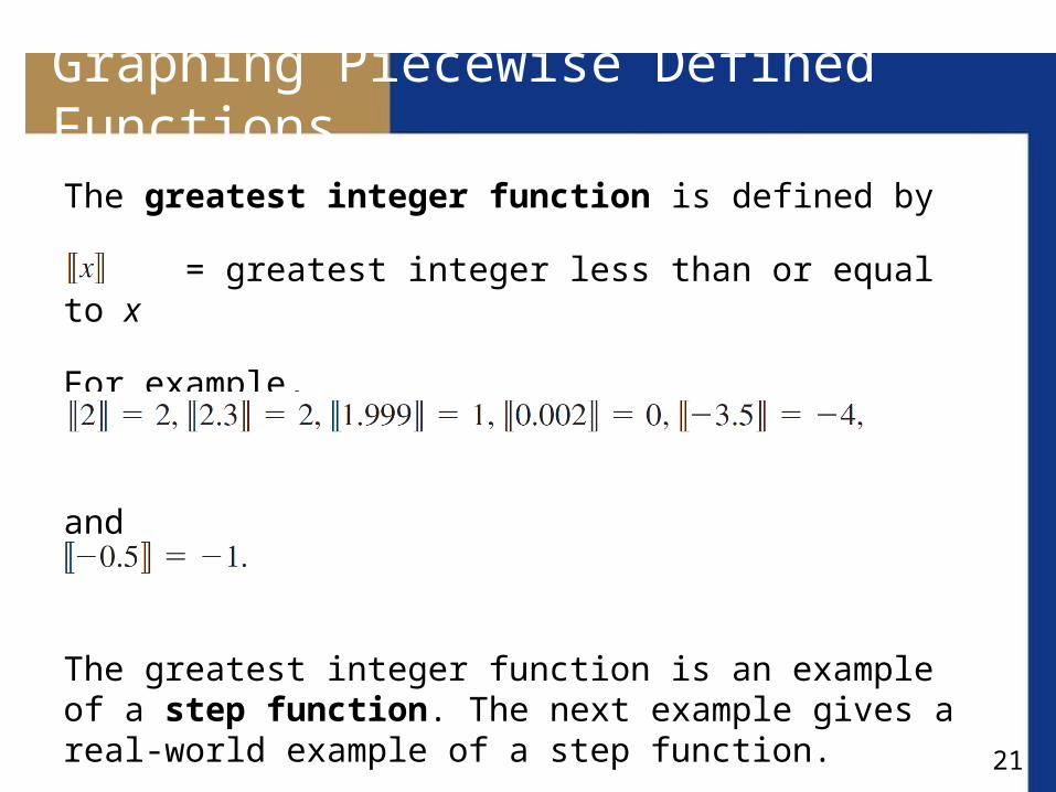
The greatest integer function is defined by

= greatest integer less than or equal to x

For example,

and

The greatest integer function is an example of a step function. The next example gives a real-world example of a step function.

22

Example 7 – The Cost Function for Long-Distance Phone Calls

The cost of a long-distance daytime phone call from Toronto, Canada, to Mumbai, India, is 69 cents for the first minute and 58 cents for each additional minute (or part of aminute).

Draw the graph of the cost C (in dollars) of the phone call as a function of time t (in minutes).

Solution:Let C (t) be the cost for t minutes. Since t > 0, the domain of the function is (0, ).

23

Example 7 – Solution

From the given information we have

C (t) = 0.69 if 0 < t 1

C (t) = 0.69 + 0.58 = 1.27 if 1 < t 2

C (t) = 0.69 + 2(0.58) = 1.85 if 2 < t 3

C (t) = 0.69 + 3(0.58) = 2.43 if 3 < t 4

and so on.

C (t) = 0.69 + 0.58

cont’d

24

Example 7 – Solution

The graph is shown in figure 9.

Cost of a long-distance call

Figure 9

cont’d

25

Graphing Piecewise Defined Functions

A function is called continuous if its graph has no “breaks” or “holes.”

The functions in Examples 1 and 2 are continuous; the functions in Examples 4 and 7 are not continuous.

26

The Vertical Line Test

27

The Vertical Line Test

The graph of a function is a curve in the xy-plane. But the question arises: Which curves in the xy-plane are graphs of functions?

This is answered by the following test.

28

The Vertical Line Test

We can see from Figure 10 why the Vertical Line Test is true.

Not a graph of a functionGraph of a function

Figure 10

Vertical Line Test

29

The Vertical Line Test

If each vertical line x = a intersects a curve only once at (a, b), then exactly one functional value is defined byf (a) = b.

But if a line x = a intersects the curve twice, at (a, b) and at (a, c), then the curve cannot represent a function because a function cannot assign two different values to a.

30

Example 8 – Using the Vertical Line Test

Using the Vertical Line Test, we see that the curves in parts (b) and (c) of Figure 11 represent functions, whereas those in parts (a) and (d) do not.

(a) (d)(c)(b)

Figure 11

31

Equations That Define Functions

32

Equations That Define Functions

Any equation in the variables x and y defines a relationship between these variables. For example, the equation

y – x2 = 0

defines a relationship between y and x. Does this equation define y as a function of x? To find out, we solve for y and get

y = x2

We see that the equation defines a rule, or function, that gives one value of y for each value of x.

33

Equations That Define Functions

We can express this rule in function notation as

f (x) = x2

But not every equation defines y as a function of x, as the next example shows.

34

Example 9 – Equations That Define Functions

Does the equation define y as a function of x?

(a) y – x2 = 2 (b) x2 + y2 = 4

Solution:(a) Solving for y in terms of x gives

y – x2 = 2

y = x2 + 2

The last equation is a rule that gives one value of y for each value of x, so it defines y as a function of x. We can write the function as f (x) = x2 + 2.

Add x2

35

Example 9 – Solution

(b) We try to solve for y in terms of x:

x2 + y2 = 4

y2 = 4 – x2

y =

The last equation gives two values of y for a given value of x. Thus, the equation does not define y as a function of x.

Subtract x2

Take square roots

36

Equations That Define Functions

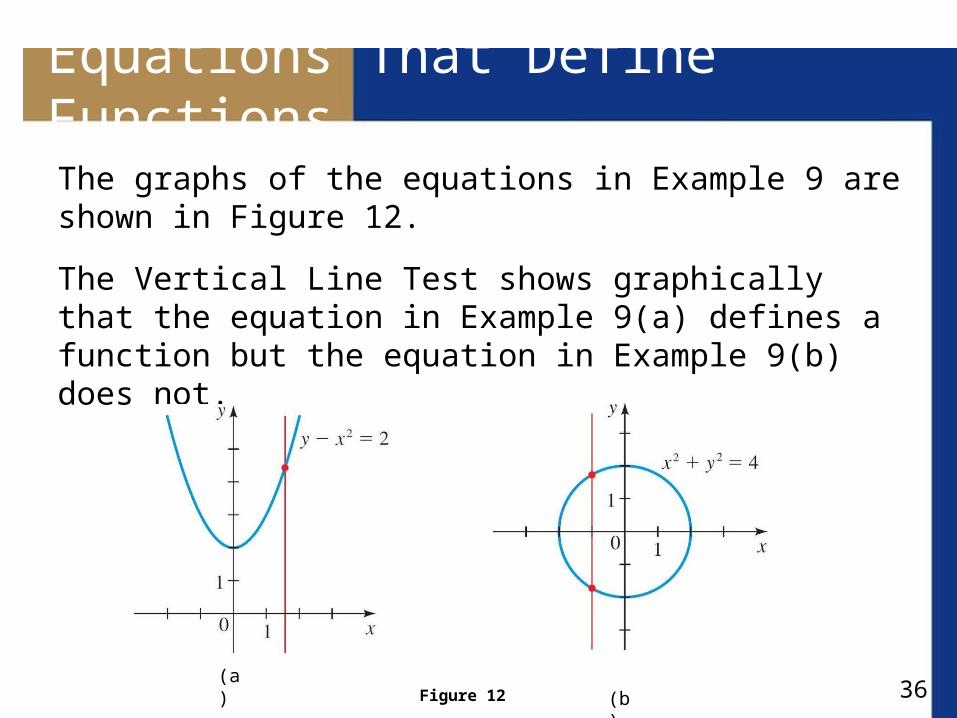
The graphs of the equations in Example 9 are shown in Figure 12.

The Vertical Line Test shows graphically that the equation in Example 9(a) defines a function but the equation in Example 9(b) does not.

(a) (b)Figure 12

37

Equations That Define Functions

The following table shows the graphs of some functions that you will see frequently.

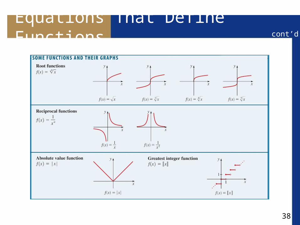
38

Equations That Define Functions

cont’d