Embed Size (px)
Citation preview

Copyright
by
Zachary James Smith
2016
A Markov Chain Model for Predicting Major League
Baseball
APPROVED BY
SUPERVISING COMMITTEE:
J. Eric Bickel, Supervisor
John Hasenbein
The Report Committee for Zachary James SmithCertifies that this is the approved version of the
following report:
A Markov Chain Model for Predicting Major League
Baseball
by
Zachary James Smith, B.S.
REPORT
Presented to the Faculty of the Graduate School of
The University of Texas at Austin
in Partial Fulfillment
of the Requirements
for the Degree of
MASTER OF SCIENCE IN ENGINEERING
THE UNIVERSITY OF TEXAS AT AUSTIN
August 2016
A Markov Chain Model for Predicting Major League
Baseball
Zachary James Smith, M.S.E.
The University of Texas at Austin, 2016
Supervisor: J. Eric Bickel
In this report, we present a Markov chain model for predicting the
scores and the winning team of Major League Baseball (MLB) games. We
discuss how a baseball game can be viewed as an infinite horizon discrete-time
Markov chain with finite state space. We demonstrate how standard Markov
chain theory can be used to obtain analytical solutions for the expected runs
and win probability in a given MLB matchup. We improve upon previous
models by incorporating pitching and more complex baserunning, and then
demonstrate the effect of these changes by comparing our model to historical
data. We also discuss computational methods for solving the model. Finally,
we test our model on games from the 2015 MLB season.
iv

Table of Contents
Abstract iv
List of Tables vi
List of Figures vii
1 Introduction . . . . . . . . . . . . . . . . . . . . . . . . . . . . 1
2 Literature review . . . . . . . . . . . . . . . . . . . . . . . . . 2
3 The expected runs model . . . . . . . . . . . . . . . . . . . . . 4
3.1 Computing expected runs . . . . . . . . . . . . . . . . . 5
3.2 Event probabilities . . . . . . . . . . . . . . . . . . . . . 5
3.3 State transitions and baserunning . . . . . . . . . . . . 14
3.4 Solving for expected runs . . . . . . . . . . . . . . . . . 18
4 The win probability model . . . . . . . . . . . . . . . . . . . . 20
4.1 Solving for win probability . . . . . . . . . . . . . . . . 21
4.2 Computational experience . . . . . . . . . . . . . . . . . 26
5 Model validation . . . . . . . . . . . . . . . . . . . . . . . . . . 28
5.1 Structural evaluation . . . . . . . . . . . . . . . . . . . 28
5.2 2015 season prediction . . . . . . . . . . . . . . . . . . . 35
6 Conclusion . . . . . . . . . . . . . . . . . . . . . . . . . . . . . 47
Appendices 49
Appendix A. Baserunning 50
1 Movement on hits and walks . . . . . . . . . . . . . . . . . . . 51
1.1 Home runs, triples and walks . . . . . . . . . . . . . . . 51
1.2 Doubles . . . . . . . . . . . . . . . . . . . . . . . . . . . 51
1.3 Singles . . . . . . . . . . . . . . . . . . . . . . . . . . . 52
2 Movement on outs . . . . . . . . . . . . . . . . . . . . . . . . . 54
2.1 Scoring from third base on an out . . . . . . . . . . . . 54
v
Appendix B. Matrices 56
1 Matrix construction . . . . . . . . . . . . . . . . . . . . . . . . 57
1.1 Expected runs . . . . . . . . . . . . . . . . . . . . . . . 57
1.2 Win probability . . . . . . . . . . . . . . . . . . . . . . 58
Bibliography 61
Vita 64
vi
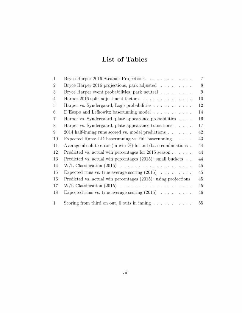
List of Tables
1 Bryce Harper 2016 Steamer Projections. . . . . . . . . . . . . 7
2 Bryce Harper 2016 projections, park adjusted . . . . . . . . . 8
3 Bryce Harper event probabilities, park neutral . . . . . . . . . 9
4 Harper 2016 split adjustment factors . . . . . . . . . . . . . . 10
5 Harper vs. Syndergaard, Log5 probabilities . . . . . . . . . . . 12
6 D’Esopo and Lefkowitz baserunning model . . . . . . . . . . . 14
7 Harper vs. Syndergaard, plate appearance probabilities . . . . 16
8 Harper vs. Syndergaard, plate appearance transitions . . . . . 17
9 2014 half-inning runs scored vs. model predictions . . . . . . . 42
10 Expected Runs: LD baserunning vs. full baserunning . . . . . 43
11 Average absolute error (in win %) for out/base combinations . 44
12 Predicted vs. actual win percentages for 2015 season . . . . . . 44
13 Predicted vs. actual win percentages (2015): small buckets . . 44
14 W/L Classification (2015) . . . . . . . . . . . . . . . . . . . . 45
15 Expected runs vs. true average scoring (2015) . . . . . . . . . 45
16 Predicted vs. actual win percentages (2015): using projections 45
17 W/L Classification (2015) . . . . . . . . . . . . . . . . . . . . 45
18 Expected runs vs. true average scoring (2015) . . . . . . . . . 46
1 Scoring from third on out, 0 outs in inning . . . . . . . . . . . 55
vii
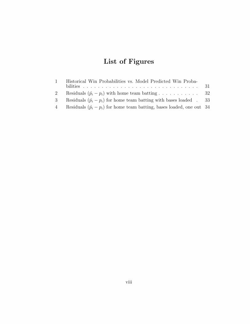
List of Figures
1 Historical Win Probabilities vs. Model Predicted Win Proba-bilities . . . . . . . . . . . . . . . . . . . . . . . . . . . . . . . 31
2 Residuals (pi − pi) with home team batting . . . . . . . . . . . 32
3 Residuals (pi − pi) for home team batting with bases loaded . 33
4 Residuals (pi − pi) for home team batting, bases loaded, one out 34
viii
1 Introduction
Baseball, or “America’s pastime”, is a sport consisting of two teams
made up of pitchers and batters. Each team has (at any one time) 8-9 po-
sition players (depending on whether a designated hitter is used), who are
responsible for hitting and fielding, and one pitcher, responsible for prevent-
ing the opposing team’s hitters from scoring runs. There are a number of
characteristics which make baseball particularly amenable to mathematical
modeling. First, at any given time, a baseball game can be in exactly one of a
finite collection of game states. In addition, the future evolution of the system
depends only on the current state and the discrete events (such as a hit) which
move the game to a new state. Furthermore, statistics and data are readily
available for estimating the player skills which determine in-game events.
The attributes described above suggest that a baseball game can be
modeled as a Markov chain. In this article, we describe a Markov chain model
for estimating runs and win probabilities for Major League Baseball (MLB)
games. In what follows, we briefly survey relevant literature, describe the
technical details of our model, discuss methods for solving the model, compare
our model’s predictions to previous models, and test our model’s performance
on games from the 2015 season.
1
2 Literature review
We briefly review some previous work which uses Markov chain mod-
els in the context of baseball. The idea for modeling a baseball game using
Markov chains dates back to at least Howard [7], who, in 1960, presented a
simple, one-inning, Markov decision process (MDP) which found the optimal
time to bunt with the goal of maximizing expected runs scored. In his famed
sabermetric tome, The Book, Tom Tango [16] presents a Markov chain ap-
proach for computing expected runs which does not account for differences in
player skills. Bukiet et al. [1] build a Markov model for predicting the distri-
bution of runs over a full game for a unique lineup of MLB player, and use it
to analyze optimization of batting orders.
Related Markov models seek to estimate win probabilities for teams in
a baseball game. In his dissertation, Null [11] uses a Markov chain framework
to predict win probabilities, and discusses how the model could be extended
to an MDP which could be used to make in-game decisions. Hirotsu and
Wright [5] present an MDP model to evaluate the optimal time to substitute
a pinch hitter. Hirotsu and Bickel [4], in an unpublished manuscript, present
an MDP model to estimate the optimal time to bunt in order to maximize
win probability or expected runs. They also note that a decision maker should
focus on the former objective, not the latter, to correctly maximize the chances
of winning.
There are also a large number of models which instead use simulation to
compute expected runs, win probabilities, and other statistics. A few examples
2
are given in [8] and [14]. This approach is used in a number of commercial
software packages.
Markov models and simulation models each have their own strengths.
A simulation model provides sampling distributions for various quantities of
interest (such as runs scored). In addition, a simulation model can more easily
track in-game changes – who specifically is on which base, substitutions, etc.
Markov chain models facilitate computation of expected values, and, generally,
can produce these results much faster than running simulations. It also allows
for simultaneous prediction for every possible state in a given game. This
feature was our primary reason for choosing the Markov chain approach – we
wanted to be able to track win probabilities during a game in real time. Finally,
as in [11] and [5], it is easy to incorporate optimal decision making within a
Markov chain model. In the following sections, we discuss our approach to
modeling a baseball game as a Markov chain.
3

3 The expected runs model
In this section, we introduce the objectives, the mathematical structure,
and the analytical solution methods for our expected runs model. A baseball
game can be fully described by a discrete set of characteristics: the current
batter and pitcher, the batter due up for the defending team, the inning, the
number of outs, the configuration of runners on the basepaths, and the score.
Given a particular state in a baseball game, our model calculates the expected
runs each team will score from that point until the end of the game.
We model a baseball game using the theory of discrete time, discrete
state space Markov chains (DTMCs). Formally, a DTMC is a stochastic pro-
cess consisting of a discrete state space S, and a stochastic transition matrix
P which describes the random movement between states in S. The transition
probabilities from a given state must adhere to the ‘Markov property,’ mean-
ing that the probability of moving from state i to state j, pij ∈ P does not
depend on the previous evolution of the system.
A baseball game fits into this framework nicely as probabilities between
game states are logically assumed to be independent of past events. For ex-
ample, suppose the game is in the bottom of the ninth inning, tied, with 2
outs and no one on base. The batter’s chances of hitting a home run – moving
the game into the “game over, home team wins” state – depend only on the
current state, the current pitcher, and the batter’s own talent, not on the par-
ticular path the game followed to reach that particular state. We now provide
more details on calculating expected runs and win probabilities.
4
3.1 Computing expected runs
We first describe the model used to compute expected runs over the
course of a 9 inning game for a given team. In reality, a team can potentially
bat in more than 9 innings if the game goes into extra innings. On the other
hand, the home team may not need to bat in the bottom of the ninth if
they already lead. However, for simplicity, when computing expected runs we
assume that a team will come up to bat 9 times during the game. As we are
only interested in one team’s performance, the elements in the state space, S,
are defined completely by:
1. The player up to bat (9 total)
2. The inning (9 total)
3. The number of outs (9 total)
4. The configuration of the baserunners on the basepaths (8 total)
There are 9 × 9 × 8 × 3 = 1944 total in-game states and a single absorbing
state, 4, representing the end of the game. We construct a 1945×1945 matrix
P which describes the evolution of the stochastic process.
3.2 Event probabilities
Transition probabilities in any state depend on the current batter, the
current pitcher, the current number of outs, and the current base configuration.
5

In our model, we assume the current batter/pitcher matchup will result in one
of the following events: single, double, triple, HR, walk/hit by pitch
(BB+HBP), double play (with < 2 outs), strikeout (K), other out
(non double play). A sequence of calculations are performed to estimate
the probabilities of these events for a given plate appearance.
We deliberately leave out a number of possible strategic baseball plays,
most notably bunts, steals, and intentional walks. These events would com-
plicate the model, as the set of possible transitions and the associated prob-
abilities when the batter decides to bunt are completely different than those
when he decides to try for a hit. In addition, treating these ‘strategic’ plays
separately allows for the possibility of adding an optimal decision making com-
ponent to our model in the future.
In each state, a pitcher from the defending team faces the hitter at the
plate. The opposing starting pitcher begins the game. After the starter exits
the game, we use the defending team’s average bullpen performance to inform
pitching for the remainder of the game. Together, the abilities of the hitter
and the pitcher inform event probabilities in a given plate appearance.
The following sequence of steps are performed to calculate these prob-
abilities. First, raw counts for batting events are obtained for both the batter
and pitcher from Steamer Projections [18] or previous season data. Using pro-
jections is the default option, as these projections consider a player’s previous
statistics, age, and other factors to forecast future performance. For exam-
ple, Steamer projects the following counting stats for Washington National’s
6

outfielder Bryce Harper for the 2016 season.
Table 1: Bryce Harper 2016 Steamer Projections.
AB 1B 2B 3B HR BB+HBP K536 94 31 2 37 110 129
Neither a player’s projections nor his past season statistics are park
neutral, meaning that, for hitters, the projections will be higher (lower) for
players who play in home stadiums which are more (less) favorable to hitters
(the opposite relations hold for pitchers). When evaluating a hitter vs. pitcher
matchup, we would like to consider their talents in a neutral environment;
thus we ‘park normalize’ the raw Steamer projections (or data) using ‘park
factors’.
Fangraphs.com [17] publishes park factors for every stadium in MLB.
Park factors describe the frequency of batting events in a given park compared
to the league average frequency. A neutral park for a given batting event,
say home runs for lefties, would have a park factor of 100. If more lefty
home runs were hit in that park compared to other stadiums, the park factor
would be greater than 100. Park factors provided by Fangraphs are specific to
the handedness of the batter. Furthermore, to facilitate calculation of park-
neutral statistics, the park factors presented on Fangraphs are adjusted down
to account for the fact that batters play only half of their games in their home
ballpark.
We divide the projected hitting statistics for both the batter and pitcher
7

by the park factors for each category. For example, if Bryce Harper is projected
to hit 37 HR in 2016, and the National’s park has a lefty-batter park factor for
HR of 92, our park-neutral projection for Harper’s HR total is 37/.92 = 38.54.
In Table 2 we show the park factors for National’s Park, along with Bryce
Harper’s adjusted hitting projections.
Table 2: Bryce Harper 2016 projections, park adjusted
1B 2B 3B HRPark factors 108 104 70 92Neutralized projection 90.4 37.25 2.35 38.54
Next, we convert the park-normalized frequency projections into event
probabilities for both the batter and pitcher. For a given batter or pitcher,
the probability of event e, where e could be a single, double, triple, home run,
walk/HBP (BB+HBP) or strikeout, is
P (e) =freq(e)
AB +BB +HBP(1)
where freq(e) is the projected frequency of event e, AB is projected at-bats,
BB is projected walks, andHBP is projected hit-by-pitches. The denominator
represents all possible considered outcomes of the plate appearance. We again
use Bryce Harper’s normalized projections for demonstration in Table 3.
Now, we need to explicitly take into consideration the handedness of the
batter and pitcher. Over large samples, hitters perform worse against pitchers
of the same handedness and better when facing opposite-handed hurlers. To
8
Table 3: Bryce Harper event probabilities, park neutral
AB 1B 2B 3B HR BB+HBP KProjected counts 536 90.4 37.25 2.35 38.54 110 129Event Probabilities .15 .05 .003 .06 .17 .2
explicitly account for this in our model, we use the ZiPS splits projections,
made available by creator Dan Szymborksi [15]. ZiPS provides full-season
statistical projections subdivided by the hand of the opposing pitcher (for
batters) and by the hand of the opposing batter (for pitchers). We use these
‘splits’ projections to compute handedness adjustment factors for each player
in the batter-pitcher matchup.
As it may be difficult to project exact statistics by handedness for
low frequency events like doubles and triples, we produce handedness splits
for the following events: Non-HR hits, HR, BB+HBP and Strikeout.
For an event e in this set, we compute the h handedness adjustment factor,
h ∈ {right, left} for e, HAh(e) as
HAh(e) =P (e|PitcherHand = h)
P (e). (2)
If a switch-hitter (a hitter who can hit both righty and lefty) is at the plate,
we assume that they will bat righty (lefty) if the pitcher is a lefty (righty).
Continuing with our example, suppose Bryce Harper is at the plate
facing righty Noah Syndergaard of the division rival New York Mets. In Table
4, we show Bryce Harper’s ZiPS projected event probabilities against righties,
9
overall, and the associated handedness adjustment factors we would apply to
his park-neutral event probabilities in Table 3.
Table 4: Harper 2016 split adjustment factors
H (non HR) HR BB+HBP Kvs. Righties .1956 .063 .181 .196Overall .1955 .0588 .176 .201Handedness adjustment 1.00 1.08 1.025 .975
Similarly, handedness adjustments would be calculated for the pitcher,
Syndergaard, reflecting his projected performance against lefties. Now, we
adjust each players projected probabilities given in Table 3 by multiplying by
the relevant handedness adjustment factors in Table 4. For example, Bryce
Harper’s park-neutral HR probability is .06. His park-neutral HR probability
against a lefty is calculated as .06× 1.08 = .064. As expected, we project that
Harper will be more likely to hit home runs against a righty pitcher.
Up to this point, we have computed projected event probabilities for
our batter and pitcher which reflect how we expect them to perform against the
league as a whole (adjusted for handedness). However, we have not considered
how the specific players in the given plate appearance will perform against each
other. We would not expect Syndergaard to perform against Bryce Harper as
he would against all other left-handed hitters, because Bryce Harper is one of
the best hitters in MLB. To derive event probabilities for the specific head-to-
head matchup, we use the so called “total Log5 rule” introduced in [3]. The
total Log5 rule generalizes the well-known Log5 rule introduced by Bill James
10
[9] to matchups involving more than two outcomes. The logical premise for
both rules is as follows: If a batter and pitcher meet, and the pitcher is worse
than the league average, we would expect the batter to perform better against
this particular pitcher than he does against the rest of the league (i.e., his
performance on average). Many baseball simulators employ similar variants
of the Log5 rule (see [8] and [14], for example).
We consider the following possible outcomes for the plate appearance
when applying the total Log5 rule: Ball-in-play (BIP), HR, BB+HBP,
K. These events are generally considered within the control of the pitcher;
once the ball is put in play, defense and luck generally determine the outcome
of the plate appearance. For an event e among these four outcomes, the Log5
probability of event e for the given plate appearance is
PLog5(e) =
pb(e)×pp(e)pl(e)∑
epb(e)×pp(e)
pl(e)
(3)
where pb(e) is the batter’s probability of generating event e, pp(e) is the
pitcher’s, and pl(e) is the leaguewide probability of event e in a plate appear-
ance with the same handedness matchup. In our example of Harper vs. Syn-
dergaard, this latter value would be the probability of event e calculated from
frequency data (as in Table 3) for all lefty-batter vs. righty-pitcher matchups
from the previous season. We use season data as opposed to the projected
league average because the projections often do not accurately predict playing
time, which can cause distortions. In addition, it is unlikely that the average
performance over hundreds of thousands of plate appearances in 2015 will be
11
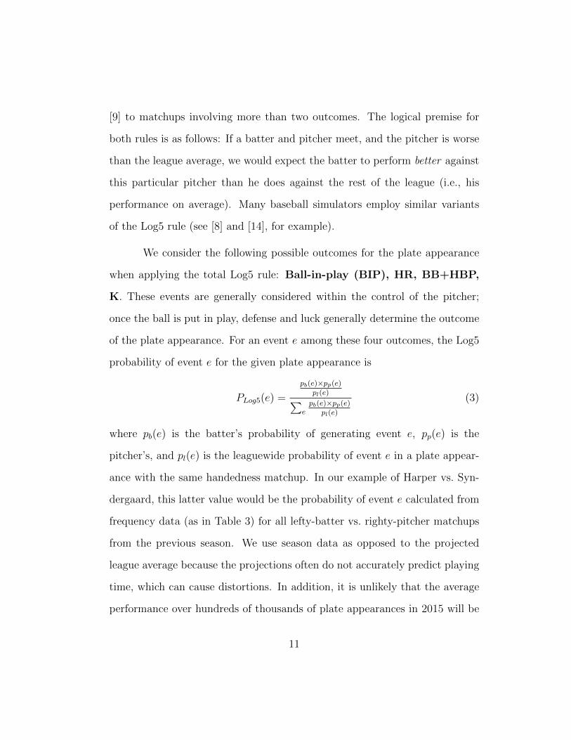
significantly different than the average in 2016.
Table 5: Harper vs. Syndergaard, Log5 probabilities
BIP HR BB+HBP KHarper .586 .064 .174 .1946Syndergaard .621 .019 .068 .292League (L vs. R) .685 .027 .096 .191Total Log5 probabilities .525 .047 .127 .303
We then distribute the log5 probability assigned to ‘BIP’ to the events
1B, 2B, 3B, Out (in play) according to the hitter’s own distribution of
events given that he puts the ball into play. For example, Bryce Harper,
against the league as a whole, is projected to put the ball in play 57% of the
time, with singles making up 26.3% of these events (see Table 3). Against
Syndergaard, per Table 5, Harper is expected to put the ball in play with
probability .525. Thus, we would estimate that he will hit a single against
Syndergaard with probability .525× .263 = .138.
We make three final adjustments to the event probabilities associated
with the plate appearance. First, we readjust for the park in which the game
is being played. For example, if the game is in National’s Park, we would
re-apply the relevant park factors for Harper. Next, we adjust for home field
advantage. Using data from the previous season (obtained from Baseball-
Reference), we compute a ‘home-field’ factor which compares the performance
of players at home compared to players in all games. For example, over the
2013 and 2014 seasons, players hit HRs in 2.39% of plate appearances in all
12
games, but 2.43% of plate appearances at home, resulting in an HR home-field
adjustment of 1.014. We would then adjust the plate appearance probabilities
in an analagous manner to handedness.
Finally, we would consider the number of hitters faced by the pitcher
prior to the given plate appearance, as pitching performance degrades over re-
peated exposure to hitters. Again, we compute “times-thru-order” adjustment
factors using full-season data from Baseball Reference. For example, in 2014,
when the hitter faced a pitcher the third time during a game, his probability of
hitting a homerun was 14% above baseline. Thus, we would increase our event
probability for an HR by 14%. We do not explicitly track the batters faced by
the starter, as this would need to be included in the state space to preserve the
Markov property. Instead, apply the adjustment factor based on the inning
in which the plate appearance takes place. Steamer provides projections for
batters faced per inning for every pitcher. Thus, we can estimate the number
of times a pitcher has gone through the order in a given state by:
Batters faced = Inning× BPI (4)
where BPI is the projected number of batters a pitcher will face per inning.
Finally, in some states it is relevant to consider double plays (we will
discuss when double plays are applicable in 3.3). We estimate the probability
of a double play for a given plate appearance using baserunning data for the
hitter from the previous season. This probability is computed from frequency
data available on Baseball-Reference, and the probability of a double play is
13

simply DP/DP Opportunities.
Having described how event probabilities for a given plate appearance
are derived, we now turn to the issue of baserunning, which determines tran-
sitions in the matrix P.
3.3 State transitions and baserunning
State transitions are determined by event probabilities, as described in
Section 3.2, combined with a baserunning model which describes the movement
of runners given certain events. For example, a single with a man on first could
result in two possible transitions. In either case, the batter will advance to
first, but the baserunner could end up on either second base or third base. We
now give a full description of our baserunning model.
Previous models (see [4], [1], [5]) have used a simplified baserunning
model proposed by D’Espopo and Lefkowitz [2] which is summarized in Table
6. After examining baserunning data, we felt that the model above fails to ad-
Table 6: D’Esopo and Lefkowitz baserunning model
Event AdvancementWalk Batter to first, baserunners advance one base if forcedSingle Batter to first, baserunners on second and third score,
baserunner on first to secondDouble Batter to second, baserunners on second and third score,
baserunner on first to thirdTriple Batter to third, all baserunners scoreHR Batter scores, all baserunners scoreOut No baserunners advance
14
equately describe the baserunning dynamics of a real MLB game. We develop
a more realistic baserunning model by adding the following:
1. Double Plays – When there are fewer than two outs, and a runner is
on first base, we consider the possibility that the batter will hit into a
double play.
2. Scoring from third base on outs – We allow a runner on third to
score on an out when the ball is put in play. We obtain the leaguewide
probabilities of scoring on an out from third for a regular ball-in-play
(BIP) out, and for a double play. We scale the probability by the batter’s
strikeout percentage, as the ball must be put in play for the runner to
reach home.
3. Runner advancement on hits – When a single is hit, we allow a run-
ner on first base to potentially advance to third base. Similarly, when
a double is hit with a baserunner on first, we allow for the possibility
that said runner will score. Finally, we assume that only some baserun-
ners score from second on a single. Statistics for individual batters for
advancements are available on Baseball-Reference and we use the team
average to inform these probabilities.
4. Runner advancement on out – We allow for the possibility that the
lead baserunner (not on third base) will advance on an out in play. We
use a single leaguewide probability for this event.
15
Other models have used different baserunning frameworks. Null [11]
calculates probabilities of transitioning from one base configuration to an-
other after a certain event by looking at leaguewide historical frequency data.
For example, given that an out occurs with one man on first, Null looks at all
historical examples of this event type and state and computes the probability
of any subsequent base state being realized. Compared to our approach, Null’s
estimates are more comprehensive; no limits are placed on the possible subse-
quent base state compositions given a certain event. However, our approach
is better for incorporating readily available team and player specific data. For
example, a team with fast runners is likely to advance from first to third on a
single more frequently than the historical frequencies would suggest, and our
baserunning model allows for those considerations.
To make the full advancement model clear, we give an example of the
transitions from a representative state. Suppose that Bryce Harper is facing
Noah Syndergaard with no outs and baserunners on first and third in the first
inning, in a game played at National’s stadium. Following Section 3.2, our
event probabilities for this plate appearance are:
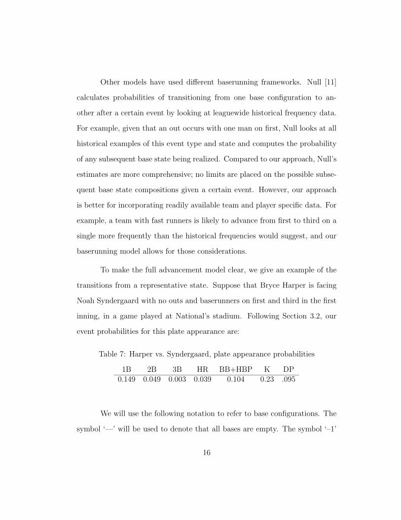
Table 7: Harper vs. Syndergaard, plate appearance probabilities
1B 2B 3B HR BB+HBP K DP0.149 0.049 0.003 0.039 0.104 0.23 .095
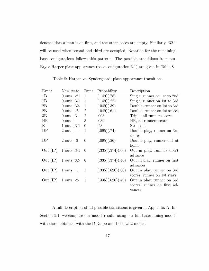
We will use the following notation to refer to base configurations. The
symbol ‘—’ will be used to denote that all bases are empty. The symbol ‘–1’
16
denotes that a man is on first, and the other bases are empty. Similarly, ‘32-’
will be used when second and third are occupied. Notation for the remaining
base configurations follows this pattern. The possible transitions from our
Bryce Harper plate appearance (base configuration 3-1) are given in Table 8.
Table 8: Harper vs. Syndergaard, plate appearance transitions
Event New state Runs Probability Description1B 0 outs, -21 1 (.149)(.78) Single, runner on 1st to 2nd1B 0 outs, 3-1 1 (.149)(.22) Single, runner on 1st to 3rd2B 0 outs, 32- 1 (.049)(.39) Double, runner on 1st to 3rd2B 0 outs, -2- 2 (.049)(.61) Double, runner on 1st scores3B 0 outs, 3– 2 .003 Triple, all runners scoreHR 0 outs, — 3 .039 HR, all runners scoreK 1 outs, 3-1 0 .23 StrikeoutDP 2 outs, — 1 (.095)(.74) Double play, runner on 3rd
scoresDP 2 outs, -2- 0 (.095)(.26) Double play, runner out at
homeOut (IP) 1 outs, 3-1 0 (.335)(.374)(.60) Out in play, runners don’t
advanceOut (IP) 1 outs, 32- 0 (.335)(.374)(.40) Out in play, runner on first
advancesOut (IP) 1 outs, –1 1 (.335)(.626)(.60) Out in play, runner on 3rd
scores, runner on 1st staysOut (IP) 1 outs, -2- 1 (.335)(.626)(.40) Out in play, runner on 3rd
scores, runner on first ad-vances
A full description of all possible transitions is given in Appendix A. In
Section 5.1, we compare our model results using our full baserunning model
with those obtained with the D’Esopo and Lefkowitz model.
17
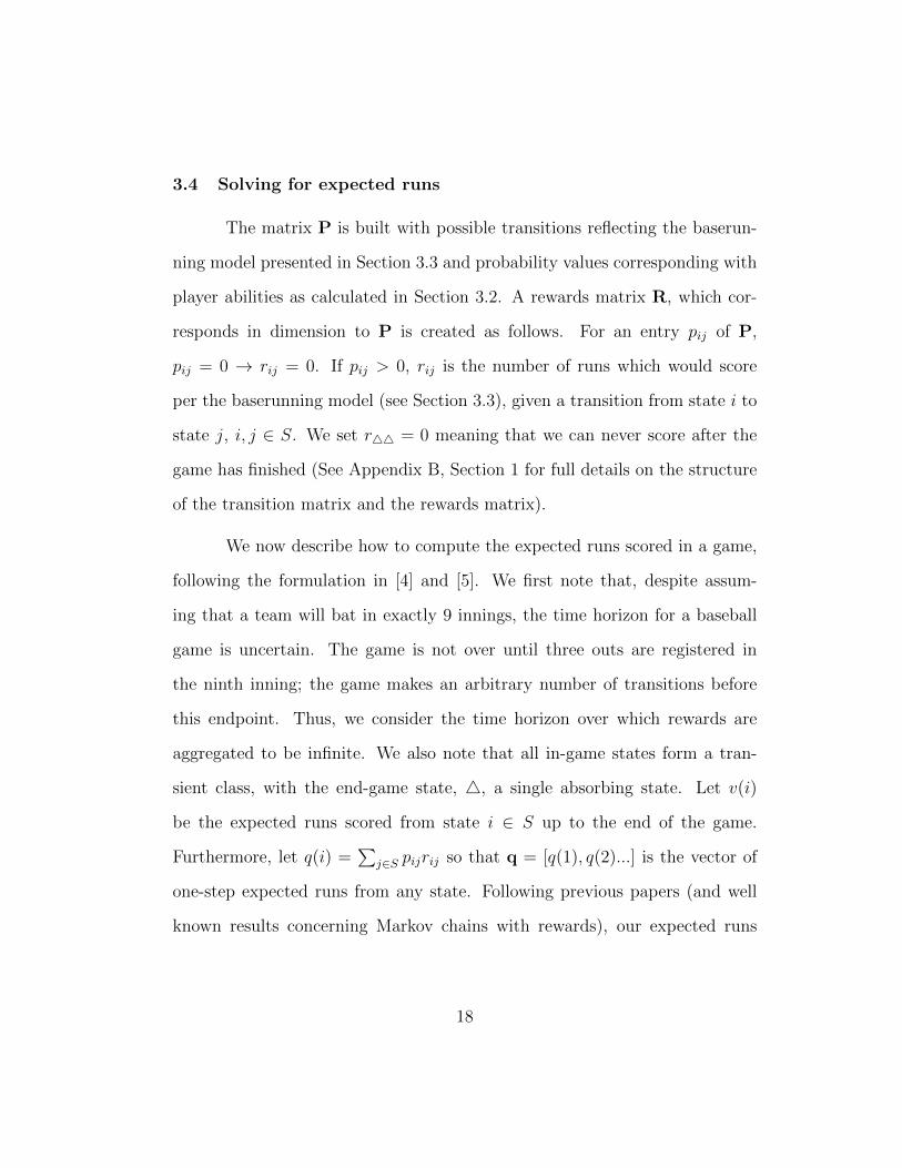
3.4 Solving for expected runs
The matrix P is built with possible transitions reflecting the baserun-
ning model presented in Section 3.3 and probability values corresponding with
player abilities as calculated in Section 3.2. A rewards matrix R, which cor-
responds in dimension to P is created as follows. For an entry pij of P,
pij = 0 → rij = 0. If pij > 0, rij is the number of runs which would score
per the baserunning model (see Section 3.3), given a transition from state i to
state j, i, j ∈ S. We set r44 = 0 meaning that we can never score after the
game has finished (See Appendix B, Section 1 for full details on the structure
of the transition matrix and the rewards matrix).
We now describe how to compute the expected runs scored in a game,
following the formulation in [4] and [5]. We first note that, despite assum-
ing that a team will bat in exactly 9 innings, the time horizon for a baseball
game is uncertain. The game is not over until three outs are registered in
the ninth inning; the game makes an arbitrary number of transitions before
this endpoint. Thus, we consider the time horizon over which rewards are
aggregated to be infinite. We also note that all in-game states form a tran-
sient class, with the end-game state, 4, a single absorbing state. Let v(i)
be the expected runs scored from state i ∈ S up to the end of the game.
Furthermore, let q(i) =∑
j∈S pijrij so that q = [q(1), q(2)...] is the vector of
one-step expected runs from any state. Following previous papers (and well
known results concerning Markov chains with rewards), our expected runs
18

vector v = [v(1), v(2), ...] satisfies:
v = Pv + q. (5)
This linear system has a unique solution once we impose the known constraint
v(4) = 0.
We now turn to the more complicated case of solving for winning per-
centages.
19
4 The win probability model
The win probability model estimates the home team’s probability of
winning at any state during the course of a baseball game. As in Section 3, we
develop a Markov chain model to solve for these probabilities. As illustrated
in previous work the state space, S, expands greatly when we are interested
in estimating the probability that the home team A will beat the away team
B from any point in a baseball game [4], [11]. Our new state space consists of:
1. The current home team player due to bat (9 possible players)
2. The current away team player due to bat (9 possible players)
3. The current batting team, or whether we are in the top or the bottom
of the inning (2 possibilities)
4. The inning (9 regular innings)
5. The number of outs in the inning (0,1, or 2)
6. The base configuration (8 possible, ranging from empty to loaded)
7. The home team’s lead, l, (l ∈ [−q, q] ∩ Z, q ∈ Z (2q + 1 possible values)
Techinically, the state space could be unbounded as there is no upper
or lower bound for the home team’s lead. However, for real games, q is finite,
practically speaking. There are competing considerations when considering
the cap, q, on the possible score differences in a game. From a computational
20

standpoint, keeping q small decreases the size of the state space, making math-
ematical operations easier. However, setting q too low leads to unintentional
bias in the model in favor of the home team. To see why, consider the ninth
inning; the home team need only achieve l > 0 to win the game, and so a cap
on the home team lead does not influence their chances of winning for any
state in the final inning. However, the visiting team must prevent the home
team from reaching this threshold. Thus, capping the amount by which the
home team can trail artificially improves the chances that the home team will
win. In our base model, we set q = 8 because, for two identical teams (without
considering home field advantage), this cap yields a projected .500 probability
of the home team winning from the beginning of the game.
We also note that the game can go into extra innings if the score is
tied at the end of the 9th. At that point, the game becomes sudden death;
if either team leads after an inning is completed, that team is the victor, or
if not, the game continues. Thus, our state space is unbounded if we were
to explicitly include all possible extra innings. However, as we show in the
following section, we need only consider one extra inning to fully solve the
model.
4.1 Solving for win probability
We can approach solving for win probability in a manner similar to
solving for expected runs scored. We build a transition matrix P, which,
considering 9 innings and a maximum lead for either team of 8, is a 594, 864×
21

594, 864 matrix. The structure of this matrix has been previously described
in [4], [5]. The baserunning model given in Section 3.3 is used to govern
transitions, and event probabilities are computed as in Section 3.2. One small
distinction is that scoring is now accounted for within the state space, as
opposed to a scoring rewards matrix as in Section 3.4.
In the Win Probability model, the home team accrues a ‘reward’ only
when a transition is made from a state i ∈ S to 4, the end-of-game state.
If the home team is leading when this transition is made, they have won the
game, and thus accrue a reward of 1. Conversely, if they are trailing when this
transition occurs, a reward of 0 is obtained. Once again let q(i) = pi4ri4 for
i ∈ S where ri4 is the reward of 0 or 1 accrued by the home team when the
game ends. Then, as before, the vector of win probabilities from any state,
w = [w(1), w(2)...], satisfies:
w = Pw + q. (6)
Again, the system has a unique solution when we impose the constraint
w(4) = 0.
Equation 6 can be thought of as a simple application of the law of total
probability, with
w(i) =∑
j∈S\4
pijw(j) + pi4ri4 (7)
where ri4 is the simply the probability of winning upon transition to the end
of game state.
22

There are a few issues with computing win probabilities by solving the
linear system in Equation 6. First, when our state space is limited to nine
innings, we must decide what reward to assign when the ninth is completed
and the game is tied. One possibility is to simply assign a reward of .5 to the
home team should the game go into extra innings. However, if one team is
significantly better than the other, this can skew computed probabilities (par-
ticularly in later innings) in an unrealistic manner. Second, solving equation
6 is a computational challenge due to the size of the matrix. We now discuss
our method for solving the model which addresses both issues.
Due to the sequential nature of a baseball game, Equation 6 can be
solved in pieces. By sequential, we mean the following: within a given inning,
we can only (potentially) transition to a later inning, and can never return to
an earlier inning. Similarly, within innings, we can only advance from the top
of the inning to the bottom, and not the other way around. One can see that
the same pattern holds for outs within half innings as well. Mathematically,
as Equation 7 makes clear, the components of vector w associated with inning
k ∈ 1, ...9 can depend only on win probability values from innings k+1, k+2...
In our model, we choose to decompose Equation 6 by inning. We begin
by solving for all extra-inning win probabilities simultaneously. Let Pextra be
the transition probability matrix for one extra inning. In this case, as we are
considering only one inning, the size of our state space is 9×9×2×8×3×17 =
66, 096 (See Appendix B, Section 2 for full details on the structure of the
transition matrix).
23
We note that all extra innings look identical in terms of computing win
percentages. A reward of either 0 or 1 is given to the home team at the end
of the inning depending on whether the home team is trailing or leading. If
the game is tied, the game transitions to another extra inning with identical
characteristics. Thus, from a modeling perspective, we can ‘transition’ to
a new extra inning by defining non-zero transition probabilities from states
at the end of the current extra inning to the beginning of the same inning.
Specifically, if we are in an extra-inning state, i, where the home team is
batting, the game is tied, there are 1 or 2 outs, with batter b ∈ 1, 2, ...9 due up
for the away team, there (may) be a non-zero probability (if an out or double
play are recorded) that the inning will end with the game tied, triggering a
new extra inning to begin. In this case, we define a nonzero entry in Pextra,
eij, where j is a state at the top of the extra with 0 outs, no men on, and
batter b at the plate.
Let qextra be the vector of one-step rewards for the extra inning, where
qextra(i) =
{pi4 Home team is leading in state i0 o.w.
}(8)
with 4 once again representing the end-of-game state. As before, we can
solve for the home team’s chances of winning from any state in extra innings
by finding the unique solution to:
wextra = Pextrawextra + qextra (9)
To solve for the rest of the game, we work backwards inning by inning.
Let 4k denote the end-of-inning state for inning k. Let Pk be the transition
24
matrix for inning k. For the ninth inning, we can easily create P9 by removing
the self loops in Pextra (along with potentially adjusting the values of the
transition probabilities). In this case, we have:
q9(i) =
pi49 Home team is leading in state ipi49wextra(i,49) Game is tied0 o.w.
. (10)
where wextra(i,49) is the win probability associated with the state in extra
innings entered upon the transition i to 49. For example, if i ={Home bat-
ter 1, Away batter 1, Bottom of 9th, 2 outs, No baserunners, Tied}, then
wextra(i,49) would be the win probability associated with the extra inning
state {Home batter 2, Away batter 1, Top of 10th, 0 outs, No baserunners,
Tied}.
For inning k, k ≤ 8, we have the following definition for the one-step
rewards vector q:
qk(i) = pi4kwk+1(i,4k). (11)
We sequentially solve the system of equations
wk = Pkwk + qk (12)
for k = 9, 8...1. Solving Equation 12 for each inning gives estimates for the
home team’s win probability from every possible state in the game.
25
4.2 Computational experience
The model, as described in Section 4.1 was implemented in Python 2.7.
There are two primary computational tasks associated with solving the model:
1. Building the matrices Pk, k = extra, 9, 8..., 1
2. Solving the systems given in equation 4.1
As the matrices are large and sparse, we make use of Python’s ScyPi sparse
matrix functionality for both constructing the matrices and solving the linear
equations.
Our decomposition approach has two computational advantages com-
pared with solving the full model simultaneously, as in Equation 6. In terms
of construction, the matrices Pk have an identical structure for each inning.
Thus, once we have built Pextra we only have to substitute new probability
values into the same matrix (to reflect a different pitcher, for example) to cre-
ate Pk, k = 9, 8, ..., 1. In addition, decomposing the problem allows for faster
solution of linear equations, as computational complexity for solving Equation
4.1 grows faster than linearly in the dimension of P.
Running the model on a MacBook Airr with a 1.4 Ghz Intel Core i5
processor, we found that, in total, building the full model and solving equation
6 takes about 33 seconds on average. In total, building the matrices and solving
the linear system sequentially, as in Equation 4.1, takes just under 10 seconds.
26

Using an iterative solver, it takes an average of 10 seconds to find the solution
for equation 6, compared to < 1 second to solve all ten systems of equations.
27
5 Model validation
There are three major components of our model which influence accu-
racy.
1. Structural – Does the hitting and baserunning model accurately reflect
a real baseball game?
2. Batter vs. Pitcher matchups – Can we accurately predict the outcome of
plate appearances with batters and pitchers of various skill levels?
3. Data and projections – Are the data and player projections used to
inform player performance accurate?
We first consider Item 1, the accuracy of our model structure.
5.1 Structural evaluation
In this section, we explore whether our structural model of a baseball
game makes sense by comparing our model to real data. By structural model,
we mean the hitting events we have chosen to consider, and the baserunning
model that dictates the movement of players. It’s worth noting that the level
of ‘modeling control’ in this structural sense is limited. For example, when an
out is made, we must move to a state with one more out, or end the current
half-inning. When the bottom of an inning is complete, we must move to a
state in the top of the following inning.
28
Thus, from a modeling perspective, we are limited in decisions on what
events to consider (i.e., should we include double plays?) and how runners
move on the basepath (i.e., does a runner on second always score on a single?).
We laid out our batting and baserunning model in detail in Sections 3.2 and 3.3,
and in Appendix A. Our limited number of structural decisions means that, for
validation purposes, we can limit ourselves to considering model performance
in predicting runs over the course of a representative half-inning.
Baseball Prospectus [20] has data on the average runs scored in a half
inning, based on the number of outs and the configuration of runners on the
bases. We downloaded the data for 2015 based on a sample of 2, 429 games.
Then, we used our model to predict expected runs within a half-inning using
a team of average 2015 batters (assumed to be competing against average
pitchers, i.e. we do not consider pitcher performance). We also compare our
model’s structural performance with earlier models using the Leftkowitz and
D’Esopo baserunning model. A comparison of our model’s predictions for
expected runs and the true data is given in Table 9.
Our model does a good job at predicting runs within a half-inning, with
no errors exceeding 1/10th of a run. We now demonstrate the benefit of our
more complex baserunning model given in Section 3.3. We perform the same
experiment as before, using the simple D’Esopo and Lefkowitz baserunning
model (we will refer to it as simply LD) in place of our own. A comparison
between the accuracy of our model and the simplified baserunning framework
is given in Table 10.
29
Our model, equipped with the full baserunning model described in Sec-
tion 3.3, outperforms the simpler baserunning model in terms of accuracy.
The largest error with the simple model is .262 runs, compared to .095 for our
model. On average, the absolute error between our model’s predictions and
the data is .031 runs, compared to .082 for the LD baserunning model. It is
not hard to see how the LD model’s limitations could cause inaccuracy. For
example, without allowing scoring from third on outs, the LD model does not
perform well in predicting runs scored when a runner is on third base with
fewer than two outs.
We also validated our model against historical win probabilities. His-
torical win probabilities for the home team for every combination of inning,
out, base configuration, and score were obtained from Greg Stoll’s Win Ex-
pectancy Finder [13]. Data was obtained from all games between 1957 and
2014 (free courtesy of retrosheet.com). As before, we used the average hitter
statistics over this time frame to inform our model, and predicted win proba-
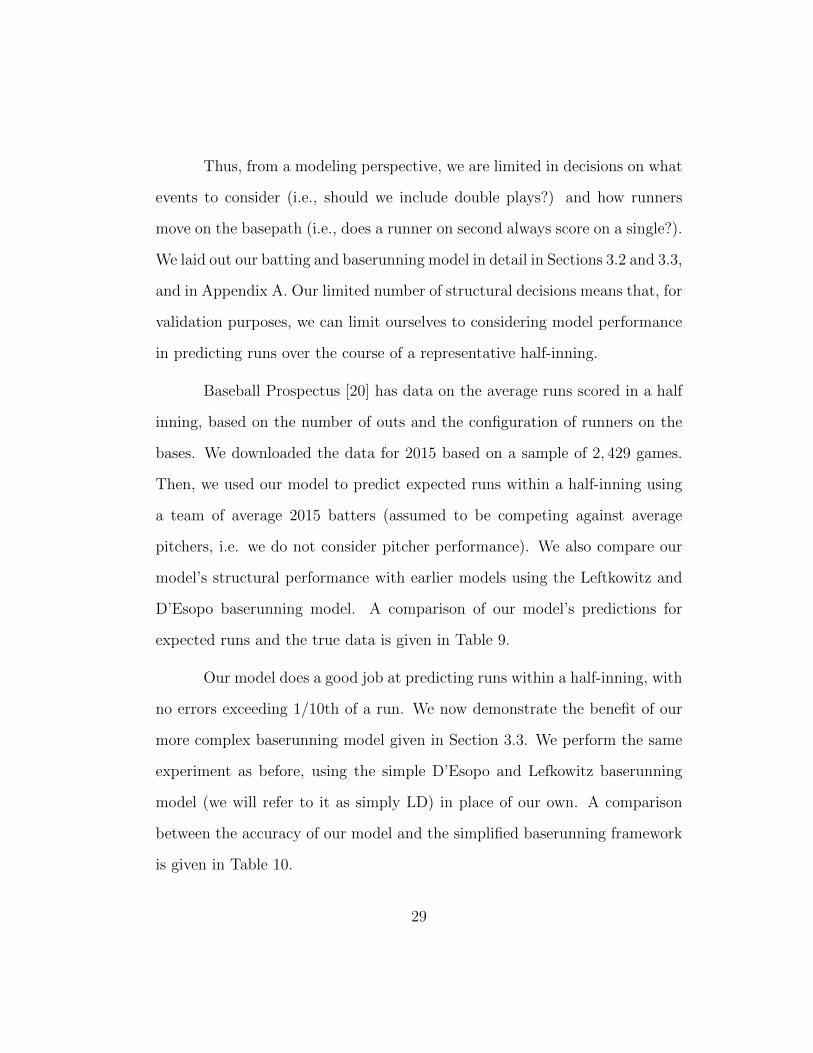
bilities. In Figure 1 we plot historical win percentages (for n = 5, 080 states
where at least 100 observations were available) against the win probabilities
calculated from our model.
In general our model performed well at predicting win probabilities.
Let pi denote the win probability predicted for the home team in state i,
and pi be the true proportion of games a home team won when state i was
reached during the game. Overall, the absolute average error between our
win probability predictions and the percentages in the data (for states with
30
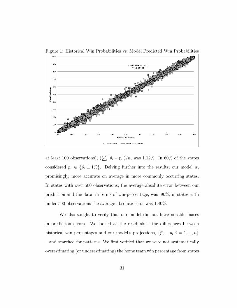
Figure 1: Historical Win Probabilities vs. Model Predicted Win Probabilities
at least 100 observations), (∑
i |pi − pi|)/n, was 1.12%. In 60% of the states
considered pi ∈ {pi ± 1%}. Delving further into the results, our model is,
promisingly, more accurate on average in more commonly occurring states.
In states with over 500 observations, the average absolute error between our
prediction and the data, in terms of win-percentage, was .90%; in states with
under 500 observations the average absolute error was 1.40%.
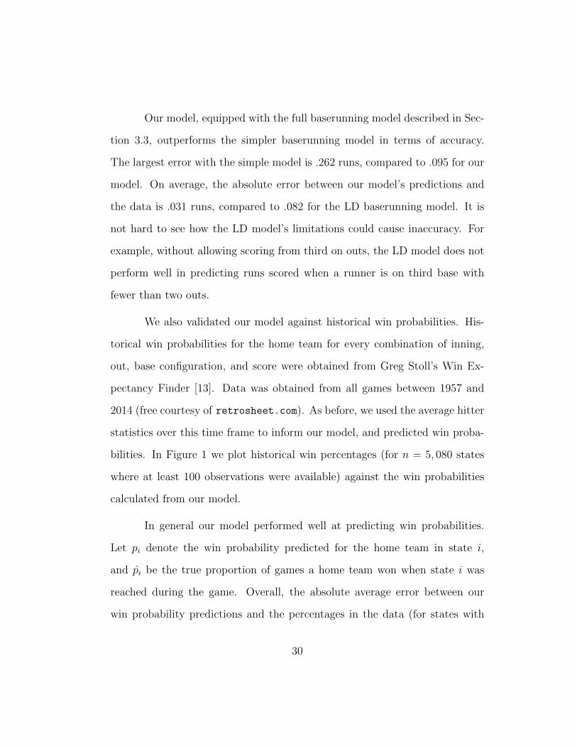
We also sought to verify that our model did not have notable biases
in prediction errors. We looked at the residuals – the differences between
historical win percentages and our model’s projections, {pi − pi, i = 1, ..., n}
– and searched for patterns. We first verified that we were not systematically
overestimating (or underestimating) the home team win percentage from states
31

in the bottom of the inning, and underestimating (or overestimating) win
percentages in the top of the inning. If this were the case, residuals as a whole
would mask the underlying flaw. We show the residuals for all states where
the home team was batting in Figure 2.
Figure 2: Residuals (pi − pi) with home team batting
We see no pattern of overestimation or underestimation in the residuals;
the average (not-absolute) residual is −.2%. We can, however, continue to
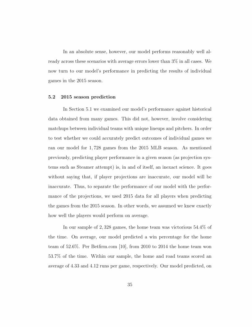
parse these results. Figures 3 and 4 show residuals for states with the home
team batting and the bases loaded, and the home team batting, bases loaded,
and 0 outs.
We see no clear patterns in the errors in either Figure 3 or Figure 4, with
average residuals of −.36% and −.62% respectively. In general, we do not find
32

Figure 3: Residuals (pi − pi) for home team batting with bases loaded
evidence that our model is systematically erroneous. Additional breakdowns
yielded similar results.
Although our model does not appear to be systematically incorrect, as
can be seen in Figure 1, this does not mean that it provides perfect predic-
tions. Reiterating our earlier point, mis-prediction is most likely to occur if
the structural baserunning model does not adequately reflect reality. In Table
11 we examine the average absolute prediction errors for various combinations
of outs and base configurations.
As shown in Table 11, the model performs worse when there are many
baserunners and a low number of outs. On the one hand, these states appear
33

Figure 4: Residuals (pi − pi) for home team batting, bases loaded, one out
in real games less frequently which means that the historical data may be
more noisy. On the other hand, higher errors in these states reflects known
limitations of our model: we don’t consider all possible baserunning outcomes,
and we don’t consider strategy (steals, bunts, intentional walks) which dictate
state transitions when runners reach base. We also do not consider differences
in hitter abilities with men on base; we use the same event probabilities when
the bases are loaded as when the bases are empty. In the real world, hitters
generally perform better as more runners are added to the basepath, because
pitchers are forced to pitch from the stretch (to prevent steals) and pound the
strikezone (to avoid walks). Adjusting hitting percentages by baserunner state
could add greater fidelity.
34
In an absolute sense, however, our model performs reasonably well al-
ready across these scenarios with average errors lower than 3% in all cases. We
now turn to our model’s performance in predicting the results of individual
games in the 2015 season.
5.2 2015 season prediction
In Section 5.1 we examined our model’s performance against historical
data obtained from many games. This did not, however, involve considering
matchups between individual teams with unique lineups and pitchers. In order
to test whether we could accurately predict outcomes of individual games we
ran our model for 1, 728 games from the 2015 MLB season. As mentioned
previously, predicting player performance in a given season (as projection sys-
tems such as Steamer attempt) is, in and of itself, an inexact science. It goes
without saying that, if player projections are inaccurate, our model will be
inaccurate. Thus, to separate the performance of our model with the perfor-
mance of the projections, we used 2015 data for all players when predicting
the games from the 2015 season. In other words, we assumed we knew exactly
how well the players would perform on average.
In our sample of 2, 328 games, the home team was victorious 54.4% of
the time. On average, our model predicted a win percentage for the home
team of 52.6%. Per Betfirm.com [10], from 2010 to 2014 the home team won
53.7% of the time. Within our sample, the home and road teams scored an
average of 4.33 and 4.12 runs per game, respectively. Our model predicted, on
35
average, that the home team would score 4.16 runs per game, and the away
team 3.88, suggesting that either our baserunning model is not adequately
representing scoring, or that we are over-emphasizing pitching skill.
In order to measure the precision of our model, we separate the predic-
tions into buckets. For example, a game where our model predicts the home
team would win 53% of the time would be grouped in the 51%− 59% bucket.
Then, for the set of games in each prediction bucket, we computed the actual
win percentage for the home team. Ideally, we would hope that in games where
the home team is predicted to win 51%− 59% of the time, they actually win
a proportion of games within that range. Table 12 shows the results of this
analysis.
As shown in Table 12, our model performs well, especially for buckets
where predictions are made most frequently. The actual observed win percent-
ages fell within each bucket in all but one case: when the model predicted a
win percentage between 35 and 43 percent, the observed win percentage was
48.57%. However, it is worth noting that evaluating results using a bucketing
approach is highly sensitive to the number of buckets, and the bucketing cutoff
values. For example, when we take smaller buckets (with sufficient numbers of
predictions) we can see that the model fidelity appears to degrade. See Table
13 for these results.
The results in Table 13 show that our model’s predictions, which look
very accurate when using large buckets, appear worse when placed under a
microscope. Unlike the results in Table 12, we no longer have a clear upward
36

trend in observed win percentages corresponding with increases in predicted
probabilities. There are a few things that are going on here. First, we are
looking at smaller sample sizes within buckets which could lead to more noisy
real world proportions. Over small to medium samples of games, unexpected
winning percentages can occur. For example, it is not uncommon for teams to
outperform their hitting fundamentals over entire seasons by stringing together
hits in high leverage situations.
But in addition, our model may not be accurate within this level of
detail. The most likely culprit for the lack of fidelity is error in assessment
of batter-pitcher matchups. As lineups in MLB are generally relatively ho-
mogeneous in talent, assessing win percentages precisely requires acurately
evaluating the effect of pitching. As noted previously, the Log5 method gives
only an approximation formula for quantifying matchup probabilities.
We made some attempt to more rigorously quantify the accuracy of our
model. Unlike a logistic regression model, grouping by features (regressors) is
not applicable for our results. When grouping by features is not possible, the
Hosmer-Lemeshow (HL) test can be used to assess fit [6]. This test assesses
model fidelity by comparing predicted successes (in our case, home team wins)
within subgroups with observed percentages. As recommended, we split our
predictions up by deciles. We then computed the HL statistic:
10∑g=1
(Og − Eg)2
Ngπg(1− πg)(13)
37
where Og are the observed wins in group g, πg is the average predicted win
probabiliy for group g, Ng is the number of observations in group g, and
Eg = πgNg. The distribution for the HL statistic approaches a chi-squared
distribution with d.f. g − 2. The HL test states that if the probability of
observing a value greater than or equal to the test statistic is less than .05 then
the model does not fit the data. The test statistic for our model’s predictions
and the true 2015 data was .049, suggesting that our predictions don’t fit the
data well.
It is worth noting, however, that the HL statistic is notoriously sensitive
to group size and group divisions. When testing our model’s predictions, this
issue came up. For example, when our predictions and the data were divided
up into 12 equally sized groups, as opposed to 10, our HL statistic was greater
than .05.
We also looked at classification rates based on our model’s predictions.
When our model gave a prediction above .5 for the home team’s win prob-
ability, we categorized that game as a win, and other games we classified as
losses. We then examined how many wins and losses we correctly predicted.
This information is presented in Table 14.
Games we classified as home team wins were actually won by the home
team 59.5% of the time. Games we classified as losses were won by the home
team 46.7% of the time. In total, our model predicted the correct outcome
57.04% of the time – more accurate than predicting the home team to win every
game. However, with our model most frequently predicting win probabilities
38
within the 45% to 60% range (reflecting the relative parity among baseball
teams), a model that is useful for baseball prediction model may not be useful
for win/loss classification.
We also compared our predictions for expected runs with the actual
score from our sample of games. Promisingly, our predictions matched up well
with the observed data. The expected runs for home teams derived from our
model and the true averages are shown in Table 15.
Again, all of the same caveats regarding bucketing apply. However,
we see a clear trend in these results: when we predicted a higher expected
run total, the average number of runs scored was indeed higher. This set of
results gives us some confidence that, at the very least, our model is properly
discerning lineup and pitching quality.
We also computed win probabilities for the same sample of 2, 328 games
using 2015 projections to inform hitter and pitcher skill. Our model predicted
on average that the home team would score 3.75 runs and the away team 3.49
runs. On average, our model predicted a win percentage of 52.8% for the home
team. One immediately notices that expected runs drop considerably when
using the projections, to well below the true scoring level in 2015. We recreate
Table 12 for the projection-based results in Table 16.
Again, even using projections to inform the model, with the larger
bucket size we appear to predict relatively accurately. At the very least, as
our model’s prediction for win probability increases, so does the observed win
39

probability. Redoing the H-L test for the projection based predictions (again
using deciles), we obtain a p-value for the test statistic of .214, suggesting that
our model fits the data. In terms of classifying wins and losses, we compare
predicted wins to actual wins in Table 17.
In this case, games we classified as a home team win were won by the
home team 59% of the time. Games we classified as a home team loss were won
by the home team 46.2% of the time. Overall, our model correctly predicts
the outcome 57.1% of the time. Finally, we repeat our comparison of expected
runs (generated by our model) and observed run scoring in Table 18.
Once again, we see that observed runs increase with our model’s pre-
dictions for expected runs. However, we underestimate runs more significantly
when we use projections. There are two potential reasons for this underesti-
mation. First, projections tend to smooth out player performances towards
the league average, which leads to less high-end run projections. Second, very
poor spot players may not have projections available and, when projections
were missing, we assumed a league average player.
The good news is that using projections appears to maintain the model’s
utility. Teams and hitters with better projections are predicted by the model
to score more runs and win more frequently, and in the aggregate they do
just that. To summarize all the results in this section: our model seems to be
fairly capable at discerning at a high level which teams are better than others.
However, further refinement (and perhaps related research into more accurate
modeling of batter-pitcher matchups) might be necessary to increase fidelity
40

further.
41
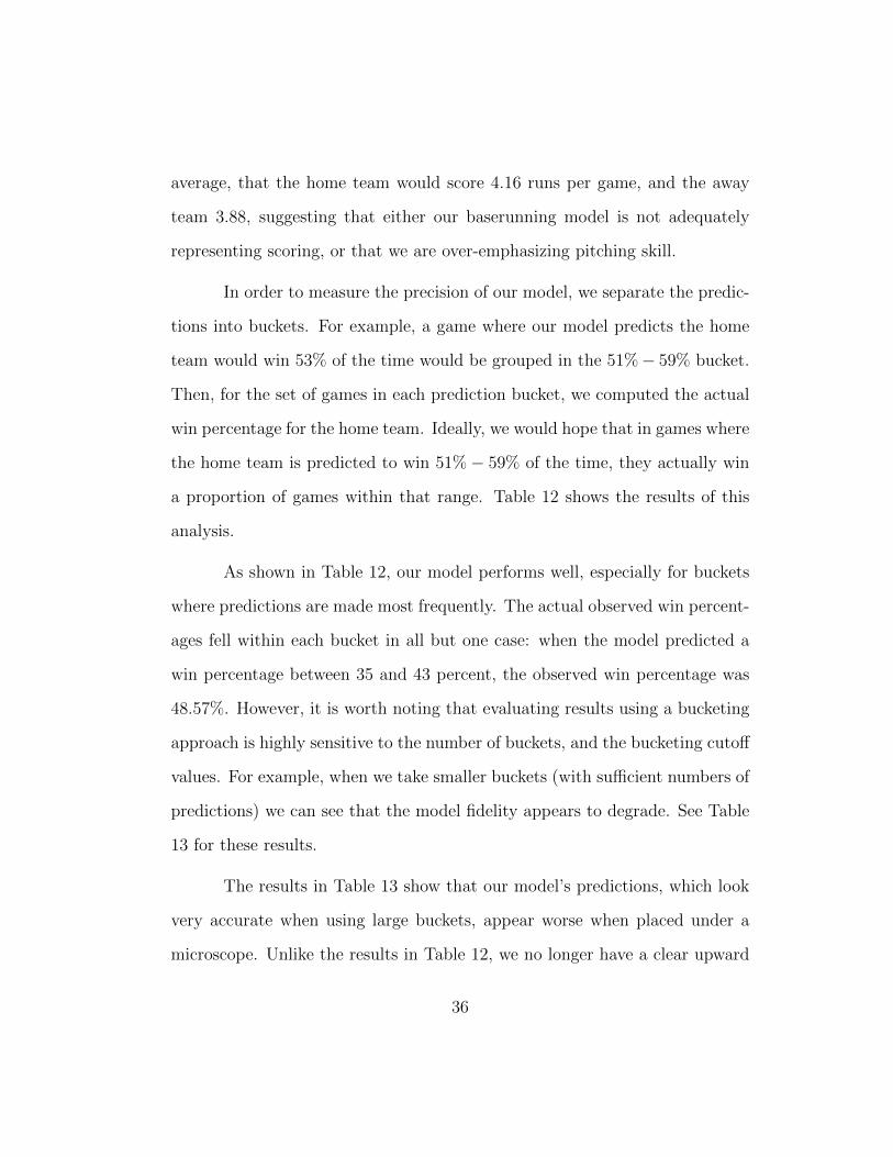
Table 9: 2014 half-inning runs scored vs. model predictions
Outs Bases Data Model WP Difference0 — 0.479 0.455 0.0240 –1 0.843 0.811 0.0320 -2- 1.076 1.04 0.0370 3– 1.305 1.317 -0.0120 -21 1.44 1.35 0.090 3-1 1.668 1.634 0.0340 32- 1.902 1.843 0.0590 321 2.265 2.171 0.0951 — 0.257 0.246 0.0111 –1 0.5 0.482 0.0181 -2- 0.649 0.63 0.0191 3– 0.892 0.925 -0.0331 -21 0.892 0.856 0.0361 3-1 1.135 1.082 0.0531 32- 1.283 1.305 -0.0221 321 1.526 1.505 0.0222 — 0.1 0.094 0.0062 –1 0.22 0.205 0.0162 -2- 0.315 0.294 0.0212 3– 0.361 0.347 0.0142 -21 0.436 0.417 0.0192 3-1 0.481 0.463 0.0192 32- 0.576 0.552 0.0242 321 0.697 0.734 -0.037
42
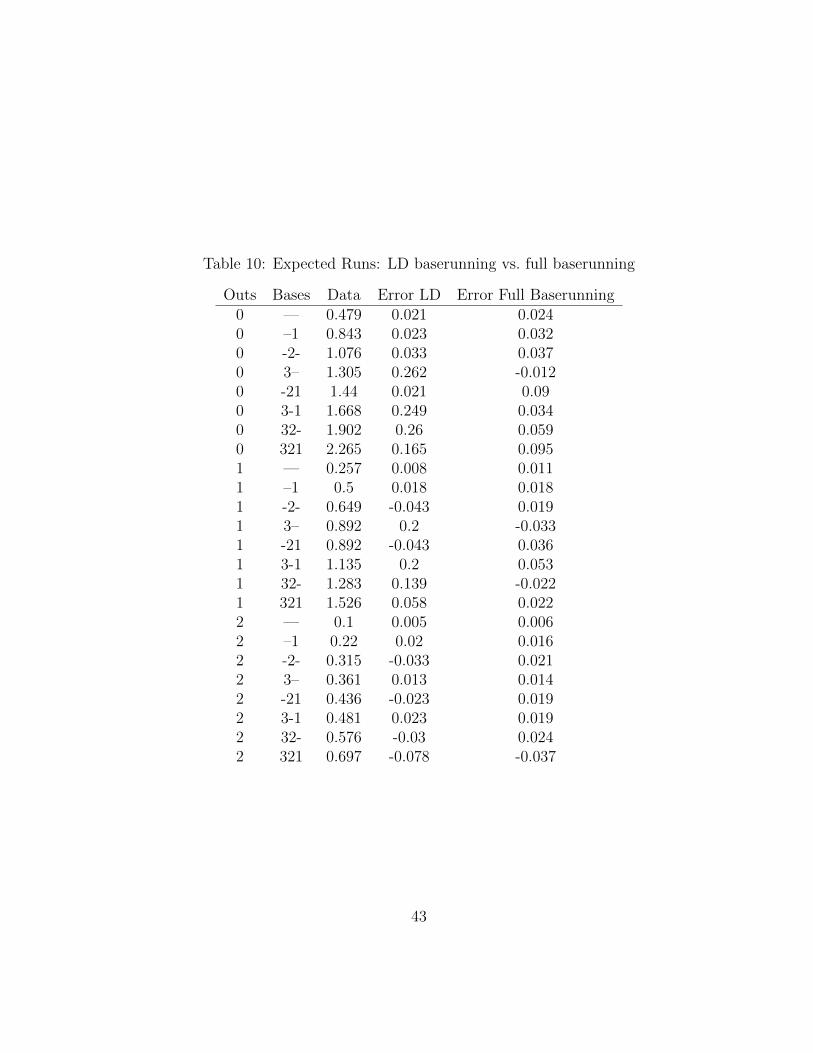
Table 10: Expected Runs: LD baserunning vs. full baserunning
Outs Bases Data Error LD Error Full Baserunning0 — 0.479 0.021 0.0240 –1 0.843 0.023 0.0320 -2- 1.076 0.033 0.0370 3– 1.305 0.262 -0.0120 -21 1.44 0.021 0.090 3-1 1.668 0.249 0.0340 32- 1.902 0.26 0.0590 321 2.265 0.165 0.0951 — 0.257 0.008 0.0111 –1 0.5 0.018 0.0181 -2- 0.649 -0.043 0.0191 3– 0.892 0.2 -0.0331 -21 0.892 -0.043 0.0361 3-1 1.135 0.2 0.0531 32- 1.283 0.139 -0.0221 321 1.526 0.058 0.0222 — 0.1 0.005 0.0062 –1 0.22 0.02 0.0162 -2- 0.315 -0.033 0.0212 3– 0.361 0.013 0.0142 -21 0.436 -0.023 0.0192 3-1 0.481 0.023 0.0192 32- 0.576 -0.03 0.0242 321 0.697 -0.078 -0.037
43

Table 11: Average absolute error (in win %) for out/base combinations
Base Config. Outs 0 1 2— 0.58 0.57 0.55–1 0.89 0.76 0.67-2- 1.08 1.08 0.923– 1.34 1.21 0.85-21 2.49 1.23 1.173-1 1.54 1.45 1.232- 2.52 1.39 1.54321 1.92 1.34 1.24
Table 12: Predicted vs. actual win percentages for 2015 season
Predicted win prob. (%) Games Avg. prediction (%) Actual win %<27 24 22.17 25
27 to 35 108 32.43 36.1135 to 43 315 40.15 48.5743 to 51 598 47.64 47.6651 to 59 635 55.16 55.5959 to 67 471 62.75 63.9167 to 75 145 70.4 71.72
75+ 32 78.58 78.13
Table 13: Predicted vs. actual win percentages (2015): small buckets
Predicted win prob. (%) Games Avg. prediction (%) Actual win %41 to 45 223 43.17 0.4745 to 49 298 46.98 0.5149 to 53 337 50.88 0.4853 to 57 339 54.92 0.5857 to 61 313 59.05 0.5661 to 65 225 63.05 0.61
44

Table 14: W/L Classification (2015)
Predict Win Predict LossWin 830 436Loss 564 498
Table 15: Expected runs vs. true average scoring (2015)
Exp. Runs n Avg. Exp. Runs. True Avg. in sample1-2 1 1.77 02-3 177 2.74 3.113-4 898 3.57 3.994-5 902 4.44 4.45-6 282 5.39 5.596+ 68 6.7 5.96
Table 16: Predicted vs. actual win percentages (2015): using projections
Predicted win prob. (%) Games Avg. prediction (%) Actual win %<32 17 0.3 0.29
32 to 39 114 0.37 0.3939 to 45 308 0.43 0.4245 to 52 633 0.49 0.5352 to 58 673 0.55 0.5558 to 64 430 0.61 0.6464 to 71 133 0.67 0.68
71+ 19 0.73 0.79
Table 17: W/L Classification (2015)
Predict Win Predict LossWin 873 393Loss 605 457
45

Table 18: Expected runs vs. true average scoring (2015)
Exp. Runs n Avg. Exp. Runs. True Avg. in sample1-2 1 1.99 02-3 266 2.76 3.823-4 1262 3.52 4.094-5 718 4.38 4.835-6 75 5.26 5.516+ 4 7.9 8.5
46
6 Conclusion
We begin our concluding remarks by discussing some limitations of our
model. While our baserunning model is more complex than some previous
examples, we certainly don’t consider a completely exhaustive list of poten-
tial transitions. For example, there are rare occasions when a runner scores
from first base when a single is hit – in our model, this transition is impossi-
ble. Further consideration of all possible transitions could potentially increase
model accuracy further, although it is worth noting that there are diminishing
returns to adding more and more possible (low probability) transitions.
In addition, our model does not have the capability of explicitly con-
sidering who is on the basepath. For example, having Dee Gordon (one of the
fastest players in baseball) on first base would considerably change the possible
transition probabilities for runner advancement. However, detailed inclusion
of unique baserunners, and their positions on the basepath, would require a
massive expansion of the state space.
There are a few limitations in our approach for incorporating pitching.
For one, we don’t consider changes in pitching performance contingent on the
configuration of runners on the base path. In reality, pitchers may pitch worse
(better) with runners on (off) base. In addition, when we make predictions
from the beginning of the game for expected runs, we have to project the
number of innings the opposing starter will remain in the game. However, this
duration is often contingent on the runs that are scored against that pitcher.
In other words, if many runs are scored, the starter will exit the game earlier;
47

our model, however, unlike a simulation model, has no way of taking this into
account. The result would be that our model might underestimate expected
runs, as relief pitchers are often worse than the starters they replace.
The Log5 method used to generate matchup probabilities for a given
batter and pitcher, is, in and of itself, an approximation. The total Log5 rule
used in our model has been shown to match observed event frequencies over
large samples of real plate appearances (see [3]). However, testing the rule
is difficult in the context of individual plate appearances, where data for a
specific pitcher and batter matchup are too few to draw inferences. Similarly,
while projection systems are remarkably accurate in the aggregate, for many
individual players they can be far off. Large projection errors for a single
player can be enough to change our model’s prediction for a given matchup.
Based on the results presented in this study, we can think of a number of
possible directions for future work. Adding in-game strategic decision making
to our model could add insight on the specific circumstances where managers
should employ bunts or steals. We could also further investigate methods
beyond Log5 for modeling batter-pitcher matchups.
Overall, our model showed promise in predicting the outcome of base-
ball games, but failed to completely capture the interaction between batters
and pitchers. We look forward to continued honing of our tool in the future.
48

Appendices
49

Appendix A
Baserunning
In this appendix, we describe completely the baserunning model pre-
sented in Section 3.3.
50

1 Movement on hits and walks
When a hit occurs, there are various possible ways runners on the
basepaths can advance. We enumerate these possibilities here.
1.1 Home runs, triples and walks
Movement on home runs and triples is simple. On a home run, re-
gardless of base configuration, all runners score including the batter himself.
Subsequently, the bases are left empty. On a triple, the batter reaches third
and all runners previously on the basepath score.
If the batter draws a walk, the batter himself advances to first. If
a baserunner is blocking his path to first, that runner advances to second,
pushing a runner on second to third, etc.
1.2 Doubles
If a double is hit, the following movement will occur. Runners on second
and third score. The batter himself reaches second. If there is a runner on first,
the runner may score, or they may reach third. Baseball-Reference provides
data for every player on how often that player scores from first base when a
double is hit. For the 2016 season, we would use baserunning data from 2015.
For each team in a given matchup, we compute a team-specific prob-
ability of a player on first scoring on a double. In a given lineup, for player
i ∈ {1, ..., 9}, let si be the number of times a player scores from first base when
a double is hit. Let si be the total number of times player i was on first base
51

when a double was hit. Then our team probability of scoring from first on a
double is:
P (Score from 1st on double) =
∑9i=1 si∑9i=1 si
. (1)
Let pdbl be the probability the batter at the plate hits a double (as
described in Section 3.2. Now, in states with a runner on first (i.e., with base
configurations –1,-21,3-1,321), the probability the runner on first scores on a
double is:
pdbl × P (Score from 1st on Double). (2)
1.3 Singles
In our model, when a single is hit, with certainty, the runner reaches
first base and a baserunner on third scores. If a runner is on either first or
second (or both), then we have a number of possibilities. A runner on second
may score or they may stop at third. A runner on first may advance to second
or may advance to third. In both cases, frequency data analagous to those
presented in Appendix A, Section 1.2 is available from Baseball-Reference for
every player. Letting ssi be the number of times player i scores from second
on a single, and ssi be the total number of times player i is on second when a
single is hit, a team probability for scoring from second on a single is calculated
as:
P (Score from 2nd on single) =
∑9i=1 ssi∑9i=1 ssi
. (3)
52
A team probability of advancing to third from first on a single is com-
puted analagously. Clearly, when runners are on first and second, the runner
on first can only reach third on a single if the runner on second has scored.
Thus, for these base states, we adjust the probability of advancement from
first to third given that the runner on second scores upwards until the overall
probability of a runner advancing from first to third matches the value in other
states.
53
2 Movement on outs
When an out is made, runners can sometimes advance. This occurs
when the ball is put into play; the runner can advance on a groundball out or
’tag up’ and advance on a fly ball out. Of course, runners can only advance
when an out does not end the half-inning.
2.1 Scoring from third base on an out
A runner on third can score on an out or a double play provided the
half-inning does not end. A runner cannot score on a strikeout. Leaguewide
frequencies for scoring from third on an in-play out (non-double play) and
on double plays are available at Baseball-Reference. Letting OS be the total
number of in-play, non-double play outs where a runner scored from third, and
O the total number of in-play, non-double-play outs, with a runner on third,
we have
P (Runner Score from 3rd|Out in play) =OS
O. (4)
Similarly, we can compute the probability a runner will score from third
on a double play. Note, this is only an applicable possibility when there are 0
outs in the inning and the configuration of runners on the bases is such that
a double play is possible – i.e. there is a runner on first. Let pout be the
current batter’s probability of making an out (any kind), pK the probability of
a strikeout, and pDP the probability of a double play. Furthermore, let po3 be
54
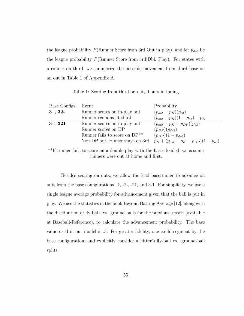
the league probability P (Runner Score from 3rd|Out in play), and let pdp3 be
the league probability P (Runner Score from 3rd|Dbl. Play). For states with
a runner on third, we summarize the possible movement from third base on
an out in Table 1 of Appendix A.
Table 1: Scoring from third on out, 0 outs in inning
Base Configs. Event Probability3–, 32- Runner scores on in-play out (pout − pK)(po3)
Runner remains at third (pout − pK)(1− po3) + pK3-1,321 Runner scores on in-play out (pout − pK − pDP )(po3)
Runner scores on DP (pDP )(pdp3)Runner fails to score on DP** (pDP )(1− pdp3)Non-DP out, runner stays on 3rd pK + (pout − pK − pDP )(1− po3)
**If runner fails to score on a double play with the bases loaded, we assumerunners were out at home and first.
Besides scoring on outs, we allow the lead baserunner to advance on
outs from the base configurations –1, -2-, -21, and 3-1. For simplicity, we use a
single league average probability for advancement given that the ball is put in
play. We use the statistics in the book Beyond Batting Average [12], along with
the distribution of fly-balls vs. ground balls for the previous season (available
at Baseball-Reference), to calculate the advancement probability. The base
value used in our model is .3. For greater fidelity, one could segment by the
base configuration, and explicitly consider a hitter’s fly-ball vs. ground-ball
splits.
55

Appendix B
Matrices
56

1 Matrix construction
In this appendix, we give the details of the matrix structures described
in Sections 3 and 4.
1.1 Expected runs
We now give the details for building the expected runs matrix. Let Pi
be the submatrix associated with the ith player in the batting order. Then
Pi is a 216 × 216 square matrix holding transitions between all innings, all
out states, and all base configurations. We organize states in our submatrix
heirarchically, with innings at the top level, outs at the second level, and
base configurations at the lowest level. Let Hj,k be the submatrix associated
with inning j with k outs which dictates transitions on a hit, and Oj,k be the
submatrix associated with transitions on outs in inning j with k outs. Then,
for i, i = 1, ..., 9
Pi =
H1,0 O1,0 O1,0 0 . . . . . . . . . . . . 00 H1,1 O1,1 O1,1 0 . . . . . . . . . 00 0 H1,2 O1,2 0 . . . . . . . . . 0...
... 0 H2,0 O2,0 O2,0 0 . . . 0...
......
.... . . . . . . . . . . . 0
0 . . . H9,0 O9,0 O9,0
0 . . . H9,1 O9,1
0 . . . 09,2
. (1)
Now, our full expected run matrix P can be written as:
57

P =
0 P1 0 . . . 0
0 0 P2 0...
......
.... . .
...0 . . . . . . . . . P8
P9 0 . . . . . . 0
. (2)
R, the one-step rewards matrix also described in Section 3 is identical in
structure to P. Entries in P are replaced with the runs scored associated with
the corresponding transition in P.
1.2 Win probability
As described in section 4, we decompose the the full matrix for the
win probability model into matrices Pk for inning k with states on each axis
ordered heirarchically by:
Home team player up (or due up)yAway team player up (or due up)y
Top/bottom of inningyOutsy
Base configurationyHome team lead (-8 to 8)
58
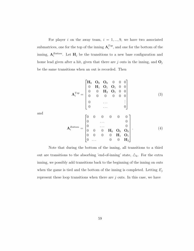
For player i on the away team, i = 1, ..., 9, we have two associated
submatrices, one for the top of the inning ATopi , and one for the bottom of the
inning, ABottomi . Let Hj be the transitions to a new base configuration and
home lead given after a hit, given that there are j outs in the inning, and Oj
be the same transitions when an out is recorded. Then
ATopi =
H0 O0 O0 0 0 00 H1 O1 O1 0 00 0 H2 O1 0 00 0 0 0 0 0
0 . . ....
0 . . . 0
(3)
and
ABottomi =
0 0 0 0 0 00 . . . 00 . . . 00 0 0 H0 O0 O0
0 0 0 0 H1 O1
0 . . . 0 0 H2
. (4)
Note that during the bottom of the inning, all transitions to a third
out are transitions to the absorbing ’end-of-inning’ state, 4k. For the extra
inning, we possibly add transitions back to the beginning of the inning on outs
when the game is tied and the bottom of the inning is completed. Letting Ej
represent these loop transitions when there are j outs. In this case, we have
59
ABottomi =
0 0 0 0 0 00 . . . 00 . . . 00 0 0 H0 O0 O0
E1 0 0 0 H1 O1
E2 0 . . . 0 0 H2
. (5)
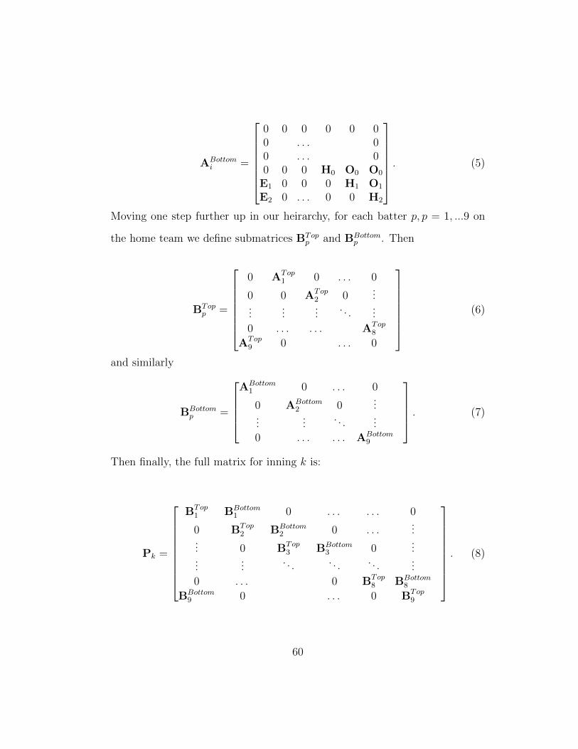
Moving one step further up in our heirarchy, for each batter p, p = 1, ...9 on
the home team we define submatrices BTopp and BBottom
p . Then
BTopp =
0 ATop
1 0 . . . 0
0 0 ATop2 0
......
......
. . ....
0 . . . . . . ATop8
ATop9 0 . . . 0
(6)
and similarly
BBottomp =
ABottom
1 0 . . . 0
0 ABottom2 0
......
.... . .
...0 . . . . . . ABottom
9
. (7)
Then finally, the full matrix for inning k is:
Pk =
BTop1 BBottom
1 0 . . . . . . 0
0 BTop2 BBottom
2 0 . . ....
... 0 BTop3 BBottom
3 0...
......
. . . . . . . . ....
0 . . . 0 BTop8 BBottom
8
BBottom9 0 . . . 0 BTop
9
. (8)
60

Bibliography
[1] Bukiet, B., Harold, E. R., & Palacios, J. L. (1997). A Markov Chain
Approach to Baseball. Operations Research, 45(1), 14-23.
[2] D’Esopo, D. A. & Lefkowitz, B. (1977) The Distribution of Runs in the
Game of Baseball. Optimal Strategies in Sports (S. P. Ladany & R. E.
Machol eds). Amsterdam: North-Holland, pp. 55-62.
[3] Haechrel, M. (2014) Matchup Probabilities in Major League Baseball.
SABR Baseball Research Journal. Available at:
http://sabr.org/research
/matchup-probabilities-major-league-baseball
[4] Hirotsu, N. & Bickel, J.E. (2014) On the Benefit of the Sacrifice Bunt:
The Importance of Differing Objectives. Manuscript submitted for pub-
lication.
[5] Hirotsu, N. & Wright, M. (2003) A Markov Chain Approach to Optimal
Pinch Hitting Strategies in a Designated Hitter Rule Baseball Game. J.
Oper. Res. Soc. Jpn., 46, 353-371
[6] Hosmer, D. W., Lemeshow, Stanley. (2013) Applied Logistic Regression:
Third Edition. Wiley.
61

[7] Howard, R. A. (1960) Dynamic Programming and Markov Processes.
Cambridge: Technology Press of the Massachusetts Institure of Technol-
ogy
[8] Hunter, Matt. (2014) 10 Lessons I Learned from Creating a Baseball
Simulator. The Hardball Times. www.hardballtimes.com
[9] James, Bill. (1983) Log5 Method. The Bill James Baseball Abstract:
12-13
[10] Jones, J. (2015, April 2) MLB Home Field Advantage. Retrieved from
http://www.betfirm.com/mlb-home-field-advantage/
[11] Null, B. (2009) Stochastic modeling and optimization in baseball. Pro-
Quest Dissertations & Theses Global.
[12] Panas, L. (2010) Beyond Batting Average. Lulu.com. 64-65.
[13] Stoll, G. Win Expectancy Finder. Retrieved from
http://gregstoll.dyndns.org
[14] Sugano, Adam P. (2008) A Player Based Approach to Baseball Simula-
tion. UCLA Statistics.
[15] Szymborski, D. (2016) ZiPS Projections. Retrieved from
twitter.com/dszymborski/status/704046976992677888
[16] Tango, T. M. (2006) The Book: Playing The Percentages In Baseball.
TMA Press.
62
[17] Handedness Park Factors (2015). Retrieved from
http://www.fangraphs.com/guts
[18] Steamer Projections. steamerprojections.com
[19] Baseball-Reference. baseball-reference.com
[20] Baseball Prospectus. baseballprospectus.com
63

Vita
Zachary Smith is an aspiring PhD student at the University of Texas
at Austin. He graduated from American University in 2013 with a degree
in Mathematics/Economics. His research involves stochastic modeling, fore-
casting, and decision analysis. He supports the Philadelphia Phillies, who
mortgaged the future to win in 2010-2011 and are now one of the worst teams
in MLB.
Permanent address: 4604 Evans AvenueAustin, Texas 78751
This report was typeset with LATEX† by the author.
†LATEX is a document preparation system developed by Leslie Lamport as a specialversion of Donald Knuth’s TEX Program.
64