Copyright by William Paul Krekelberg 2008

Copyright

by

William Paul Krekelberg

2008

The Dissertation Committee for William Paul Krekelberg

certifies that this is the approved version of the following dissertation:

Relationships between structure and dynamics

of attractive colloidal fluids

Committee:

Thomas M. Truskett, Supervisor

Venkat Ganesan, Supervisor

Isaac C. Sanchez

John G. Ekerdt

David Vanden Bout



by

William Paul Krekelberg, B.S.

Dissertation

Presented to the Faculty of the Graduate School of

The University of Texas at Austin

in Partial Fulfillment

of the Requirements

for the Degree of

Doctor of Philosophy


August 2008

Dedicated to MP and CTD

Acknowledgments

Foremost, I would like to thank my advisors Thomas Truskett and Venkat

Ganesan for providing an outstanding research environment and inputs on

every aspect of this work. Their knowledge of a wide variety of topics helped

mold this dissertation. Thank you both for all your help and for putting up

with me over the years.

Much of my time was spent interacting with members of the Truskett

and Ganesan groups. Thank you all for the discussions on science, sports, and

everything else. Thanks Gaurav for the collaborations. A special thanks to

Jeetain for very influential discussions, which motivated much of the work in

this thesis.

The National Science Foundation graciously supported my studies through

a Graduate Research Fellowship. This independent funding made possible the

study of a diverse range of topics.

Finally, I would like to thank my family for their support of me being

me.

William Paul Krekelberg


August 2008

v



Publication No.

William Paul Krekelberg, Ph.D.

The University of Texas at Austin, 2008

Supervisors: Thomas M. Truskett and Venkat Ganesan

Relationships between structure and dynamics in fluids have a wide variety of

applications. Because theories for fluid structure are now well developed, such

relationships can be used to “predict” dynamic properties. Also, recasting

dynamic properties in terms of structure may provide new insights. In this

thesis, we explore whether some of the relationships between structure and

dynamics that have proven useful for understanding simple atomic liquids can

also be applied to complex fluid systems. In particular, we focus on model

fluid systems with particles that interact with attractive forces that are short-

ranged (relative to the particle diameter), and display properties that are

anomalous when compared to those of simple liquids. Examples of fluids with

short-range attractive (SRA) interactions include colloidal suspensions and

solutions of micelles or proteins.

vi

We show via simulations that common assumptions regarding free vol-

ume and dynamics do not apply for SRA fluids, and propose a revision to

the traditional free volume perspective of dynamics. We also develop a model

which can predict the free volume behavior for hard-sphere and SRA fluids.

Next, we demonstrate that the dynamic properties of SRA fluids can

be related to structural order. In terms of structural order, the properties of

SRA fluids can be related to those of another anomalous fluid, liquid water. In

both fluids, anomalous dynamics are closely related to anomalous structure,

which can be traced to changes in second and higher coordination shells. We

also find that a similar relationship between structural order and dynamics

approximately holds for fluids under shear.

Motivated by previous work, we explore via simulation how tuning the

particle-wall interactions to flatten or enhance the particle layering in a con-

fined fluid impacts its self-diffusivity, viscosity, and entropy. We find that the

excess entropy explains the observed trends.

Finally, we present preliminary simulation data regarding the relation-

ship between heterogeneous dynamics and structure. We show that the mo-

bility of particles is related in a simple way to the structure of the particles

surrounding them. In particular, our results suggest that a critical amount of

local disorder allows a particle to be mobile on intermediate time scales.

vii

Contents

Acknowledgments v

Abstract vi

List of Figures xi

Chapter 1 Introduction 1

1.1 Relating dynamics to structure . . . . . . . . . . . . . . . . . 2

1.1.1 Free Volume and dynamics . . . . . . . . . . . . . . . . 2

1.1.2 Structural order and dynamics . . . . . . . . . . . . . . 3

1.2 Complex dynamic properties of fluids . . . . . . . . . . . . . . 4

1.2.1 Anomalous dynamics of short-ranged attractive fluids

and re-entrant glass transition . . . . . . . . . . . . . . 5

1.2.2 Fluids under shear . . . . . . . . . . . . . . . . . . . . 10

1.2.3 Confined fluids . . . . . . . . . . . . . . . . . . . . . . 11

1.2.4 Structure and heterogeneous dynamics . . . . . . . . . 11

1.3 Thesis organization . . . . . . . . . . . . . . . . . . . . . . . . 12

Chapter 2 Free Volumes and the anomalous self-diffusivity of

attractive colloids 17

2.1 Introduction . . . . . . . . . . . . . . . . . . . . . . . . . . . . 17

2.2 Methods . . . . . . . . . . . . . . . . . . . . . . . . . . . . . . 19

2.2.1 Model fluid . . . . . . . . . . . . . . . . . . . . . . . . 19

2.2.2 Free volume . . . . . . . . . . . . . . . . . . . . . . . . 21

2.3 Results and discussion . . . . . . . . . . . . . . . . . . . . . . 22

2.4 Conclusions . . . . . . . . . . . . . . . . . . . . . . . . . . . . 31

viii

Chapter 3 Model for the free-volume distributions of equilib-

rium fluids 32

3.1 Introduction . . . . . . . . . . . . . . . . . . . . . . . . . . . . 32

3.2 General Framework . . . . . . . . . . . . . . . . . . . . . . . . 34

3.3 Testing the model . . . . . . . . . . . . . . . . . . . . . . . . . 38

3.3.1 Predictions for the HS fluid . . . . . . . . . . . . . . . 38

3.3.2 Simulations of the HS Fluid . . . . . . . . . . . . . . . 42

3.3.3 Predictions for the Square-Well Fluid . . . . . . . . . . 48

3.3.4 Simulations of the Square-Well Fluid . . . . . . . . . . 49

3.4 Conclusions . . . . . . . . . . . . . . . . . . . . . . . . . . . . 52

Chapter 4 How short-range attractions impact the structural

order, self-diffusivity, and viscosity of a fluid 53

4.1 Introduction . . . . . . . . . . . . . . . . . . . . . . . . . . . . 53

4.2 Modeling and Simulation . . . . . . . . . . . . . . . . . . . . . 56

4.3 Results and Discussion . . . . . . . . . . . . . . . . . . . . . . 58

4.3.1 Transport and Structural Properties . . . . . . . . . . 58

4.3.2 Connection between structure and mobility anomalies . 67

4.3.3 Structure-property relations and the breakdown of Stokes-

Einstein . . . . . . . . . . . . . . . . . . . . . . . . . . 70

4.4 Conclusions . . . . . . . . . . . . . . . . . . . . . . . . . . . . 79

Chapter 5 Structural anomalies of fluids: Origins in second and

higher coordination shells 81

5.1 Introduction . . . . . . . . . . . . . . . . . . . . . . . . . . . . 81

5.2 Methods . . . . . . . . . . . . . . . . . . . . . . . . . . . . . . 86

5.2.1 Waterlike fluid models . . . . . . . . . . . . . . . . . . 86

5.2.2 SRA fluid models . . . . . . . . . . . . . . . . . . . . . 89

5.2.3 Quantification of structural order . . . . . . . . . . . . 90

5.3 Structural anomalies . . . . . . . . . . . . . . . . . . . . . . . 91

5.3.1 Waterlike fluids . . . . . . . . . . . . . . . . . . . . . . 91

5.3.2 SRA fluids . . . . . . . . . . . . . . . . . . . . . . . . . 99

ix

5.4 Conclusions . . . . . . . . . . . . . . . . . . . . . . . . . . . . 104

Chapter 6 Relationship between shear viscosity and structure

of a model colloidal suspension 108

6.1 Introduction . . . . . . . . . . . . . . . . . . . . . . . . . . . . 108

6.2 Methods . . . . . . . . . . . . . . . . . . . . . . . . . . . . . . 112


6.3.1 Shear viscosity . . . . . . . . . . . . . . . . . . . . . . 113

6.3.2 Free volume and the correlation to shear viscosity . . . 115

6.3.3 Structural order and the correlation to viscosity . . . . 120

6.3.4 Lennard-Jones Fluid . . . . . . . . . . . . . . . . . . . 125

6.4 Conclusions . . . . . . . . . . . . . . . . . . . . . . . . . . . . 127

Chapter 7 Tuning density profiles and mobility of inhomoge-

neous fluids 128

7.1 Introduction . . . . . . . . . . . . . . . . . . . . . . . . . . . . 128

7.2 Methods . . . . . . . . . . . . . . . . . . . . . . . . . . . . . . 130

7.2.1 Model fluid . . . . . . . . . . . . . . . . . . . . . . . . 130

7.2.2 Tuning density profiles and excess entropy . . . . . . . 131

7.2.3 Simulations methods . . . . . . . . . . . . . . . . . . . 133


7.4 Conclusions . . . . . . . . . . . . . . . . . . . . . . . . . . . . 138

Chapter 8 Structural and dynamic heterogeneities 139

8.1 Introduction . . . . . . . . . . . . . . . . . . . . . . . . . . . . 139

8.2 Methods . . . . . . . . . . . . . . . . . . . . . . . . . . . . . . 140


8.3.1 Quantifying dynamic heterogeneities . . . . . . . . . . 141

8.3.2 Structure of mobile and immobile particles. . . . . . . 146

8.4 Conclusions . . . . . . . . . . . . . . . . . . . . . . . . . . . . 152

Bibliography 155

x

Vita 173

xi

List of Figures

1.1 Dynamical transitions for fluid composed of particles with short-ranged attractions. The glass lines separate the “liquid” regionsfrom the “glass” regions. The vertical black dashed line repre-sents the hard-sphere glass line. In the case of short-range at-tractive colloids [15, 16], the re-entrant (non-monotonic) shapeof the glass line (solid red and blue lines) creates a pocket ofliquid states that are stabilized by the short-range attraction.The location of the theoretical glass-glass transition line (thickblue line) and the proposed connection between the gel-line (atlow volume fractions) and the attractive glass line (solid blueline) are also indicated. Equilibrium (and metastable) coexis-tence curves between liquid and solid phases – which in the caseof attractive colloids are significantly different from the caseof simple fluids with long-range attractions – are not shown.(Adapted from Ref. [13]) . . . . . . . . . . . . . . . . . . . . . 7

1.2 Effect of increasing the polymer volume fraction ϕRpolymer on the

structural relaxation time τα at colloid volume fraction ϕcolloid =0.67. The vertical lines schematically indicate the transitionslines to the respective glassy states. (Adapted from [15]) . . . 9

2.1 Effective colloidal pair potential of the model SRA fluid USRA(r)discussed in the text for various values of nonadsorbing polymerconcentration φp. . . . . . . . . . . . . . . . . . . . . . . . . . 20

2.2 Two-dimensional schematic of particles (black circles) with ex-clusion disks (grey circles). The free volume of the shaded par-ticle (left) is equal to the local connected volume of particle-center-accessible space that would be formed if the particle wereremoved from the configuration (i.e., the cavity indicated by thehatched region, right). . . . . . . . . . . . . . . . . . . . . . . 21

2.3 HS reference fluid. (a) Self-diffusivity D versus particle volumefraction φc. (b) Average free volume 〈vf〉 versus particle volumefraction φc. (c) Self-diffusivity D versus average free volume 〈vf〉. 23

xii

2.4 SRA fluid (a) Self-diffusivity D versus polymer volume fractionφp. (b) Average free volume 〈vf〉 versus polymer volume frac-tion φp at particle volume fractions φc = 0.4, 0.5, and 0.55.(c) Free volume size distribution p(vf) at φc = 0.4 for theHS reference fluid and the SRA fluid at (following the arrow)φp = 0.1, 0.2, 0.3, and 0.4. Dotted lines indicate boundariesof free volume regions (see text). Qualitatively similar distribu-tions occur for φc = 0.5 and 0.55 (not shown) (d) Self-diffusivityD versus average free volume 〈vf〉 for the HS reference fluid(open circles) and the SRA fluid at φc = 0.4 (closed circles),φc = 0.5 (closed triangles), and φc = 0.55 (closed squares). . . 25

2.5 Free volume autocorrelation function Cvfversus time t for (a)

the HS reference fluid (arrow indicates increasing φc) and (b)the SRA fluid (arrow indicates increasing φp). Lower panel:free volume persistence times τf calculated by fitting Cvf

to theform Cvf

(t) = Afe−t/τf + Ave

−t/τv + AGe−(t/τG)2/2 (subscripts v

and G denote the vibrational and Gaussian contributions, re-spectively) for (c) the HS reference fluid as a function of par-ticle volume fraction φc and (d) the SRA fluid as a functionof polymer volume fraction φp at φc = 0.4 (circles), φc = 0.5(triangles), and φc = 0.55 (squares). For all cases studied forboth models, τf was found to be larger than τv by an order ofmagnitude or more. . . . . . . . . . . . . . . . . . . . . . . . . 28

2.6 Comparison of self-diffusivity D (closed symbols) to that esti-

mated using the relation D = C〈vf〉2/3/τf (open symbols) for

(a) the SRA fluid as a function of polymer volume fraction φp

at particle volume fraction φc = 0.4 (circles), φc = 0.5 (trian-gles), and φc = 0.55 (squares) and for (b) the HS reference fluidas a function of particle volume fraction φc. The parameter Cdoes not depend on φp or φc, and it was chosen for each modelto provide a reasonable overall fit to the simulation data. . . 30

3.1 A 2D schematic of the free volume of a tagged particle. Overlap-ping grey circles represent the exclusion spheres of the neighbor-ing particles. (a) The small dashed circle is the tagged particlesurface, and the larger dashed circle is its associated exclusionsphere. The cross-hatched region is the tagged particle’s freevolume. (b) An expanded view of the tagged particle’s freevolume along with its approximate representation in our model. 36

xiii

3.2 (a) Free-volume distributions of the 3D HS fluid for packingfractions φc = 0.375, 0.4, 0.425, 0.45, 0.475, 0.5 and 0.525. Sym-bols are simulation data and solid curves are the predictions ofEq. (3.2). The arrow indicates increasing packing fraction φc.Inset: Average free volume 〈vf〉 versus packing fraction φc. Cir-cles are simulation data and the solid line is the prediction ofEq. (3.15). (b) Probability density associated with observingparticles with scaled free volume v∗f = vf/〈vf〉. Symbols aresimulation data from panel (a) and the solid line is the predic-tion of Eq. (3.18). . . . . . . . . . . . . . . . . . . . . . . . . . 44

3.3 (a) Proabability density associated with observing particles withscaled free surface area s∗f = sf/〈sf〉 in the 3D HS fluid for pack-ing fractions φc = 0.375, 0.4, 0.425, 0.45, 0.475, 0.49, 0.5, 0.51,and 0.525. Symbols are simulation data and solid curves are thepredictions of Eq. (3.20). Inset: Average free surface area 〈sf〉versus packing fraction φc. Circles are simulation data and thesolid line is the prediction of Eq. (3.16). (b) Average sphericity〈λf〉 of free volumes in the HS fluid versus packing fraction φc.Circles are simulation data, and the solid line is the predictionof Eq. (3.22). . . . . . . . . . . . . . . . . . . . . . . . . . . . 45

3.4 Equation of state for the HS fluid as calculated from bothEq. (3.25) and the Carnahan-Starling [62] relationship. In-set: Expanded version illustrating that Eq. (3.25) diverges atφc,MRJ = 0.64, while the Carnahan-Starling relationship di-verges at the unphysically high packing fraction of φc = 1. . . 47

3.5 Free-volume distributions for the square-well fluid at range ofattraction ∆ = 0.03, and reduced second virial coefficients B∗

2 =−0.04, 0.41, 0.60, 0.78, 0.84, 0.91 and 0.94. (a) Simulations atpacking fraction φc = 0.5 and (b) the free-volume model atdescribed in the text at φc = 0.5. (c) Simulations at packingfraction φc = 0.58 and (d) free-volume model at φc = 0.58.Arrows indicate increasing B∗

2 . . . . . . . . . . . . . . . . . . . 51

xiv

4.1 Transport properties of the HS fluid described in the text as afunction of packing fraction φc: (a) self-diffusivity D, (b) vis-cosity η, and (c) SE relationship Dη/T . The horizontal dashedline in (c) indicates (2π)−1, the expected value of the SE rela-tion in the slip limit, and the vertical line denotes the point atwhich which Dη = 1.2/(2π). In this work, we use this simpleheuristic to identify the breakdown of the SE relation. . . . . . 59

4.2 Transport properties of the SW-SRA fluid described in the textas a function of packing fraction φc and reciprocal temperatureT−1: (a) self-diffusivity D, (b) viscosity η, and (c) SE relation-ship Dη/T . The horizontal dashed line in (c) indicates (2π)−1,the expected value of the SE relation in the slip limit. . . . . . 61

4.3 Structural properties of the HS fluid discussed in the text. (a)Translational structural order parameter −s2 versus packingfraction φc. (b) Radial distribution function g(r) for severalpacking fractions. (c) Cumulative order integral (see Eq. 4.3).Arrows indicate increasing φc. . . . . . . . . . . . . . . . . . . 63

4.4 Structural properties of the SW-SRA fluid. (a) Structural orderparameter −s2 versus reciprocal temperature T−1. Symbols arethe same as in Fig. 4.2. (b) Radial distribution function g(r) and(c) cumulative order integral Is2

(r) for φc = 0.55 and T ≤ 0.4.(d) Radial distribution function g(r) and (e) cumulative orderintegral Is2

(r) for φc = 0.55 and T ≥ 0.4. . . . . . . . . . . . 654.5 Conditions exhibiting self-diffusivity and structural anomalies,

as well as breakdown of the SE relation [Dη/T > 1.2/(2π), seediscussion in text] for the SW-SRA fluid in the T -φc plane. (a)Results from simulations. Large closed circles are state pointswhere the SE relationship breaks down. Open circles representthe region of structural anomalies defined by Eq. (4.5). Smallclosed circles represent the region of self-diffusivity anomaliesdefined by Eq. (4.4). (b) Schematic representation of the data.The green shaded region (and area to its right) represents statepoints where the fluid is structurally anomalous. The blueshaded region represents state points exhibiting the self-diffusivityanomaly. Points to the right of the red curve show a breakdownof the SE relation. The gray region represents the repulsive andattractive glassy states. . . . . . . . . . . . . . . . . . . . . . . 68

xv

4.6 Transport properties as a function of structural order parameter−s2 for the HS fluid described in the text. (a) Self-diffusivity D,(b) viscosity η, and (c) the SE relationship. In (a) and (b), theblue and red lines represent fits to Eq. 4.6 for the equilibriumand supercooled states, respectively. . . . . . . . . . . . . . . . 72

4.7 (a) Scaled self-diffusivity DT−1/2, (b) scaled viscosity ηT−1/2,and (c) SE relationship Dη/T versus structural order parameter−s2 for the SW-SRA fluid at several packing fractions φc. Self-diffusivity D, viscosity η, and the SE relationship Dη for theHS fluid are provided for comparison. Filled and open symbolsrepresent the high (T > 0.5) and low (T < 0.5) temperaturebranches of the SW-SRA fluid, respectively. Dashed lines in (a)and (b) are fits of the SW-SRA data to Eq. (4.6) and the dashedlines in (c) are the products of the respective fits in (a) and (b).Arrows in (a) indicate the general direction of increasing T . Redand blue lines have the same meaning as those in Fig. 4.6. . . 75

4.8 Values of the coupling coefficients B′D and −B′

η from fits of thesupercooled SW-SRA data to Eq. (4.6) (shown in Fig. 4.7) forthe self-diffusivity D and viscosity η, respectively. Also shownare the (negative) sum −(B′

D +B′η) and the ratio −(B′

η/B′D) of

the exponents. The dashed line represents the HS fluid valuefor −(B′

η/B′D) . . . . . . . . . . . . . . . . . . . . . . . . . . . 77

4.9 (a) Schematic representing a speculation about how the scaledself-diffusivity vs −s2 isochores of the SW-SRA fluid [Fig. 4.7(a)]might behave as the repulsive and attractive glass transitionsare approached. The quantities s2,R and s2,A represent the lim-iting values of s2 for the repulsive and attractive glasses, respec-tively. (b) The black and red curve are the proposed iso-s2 lociin the T − φc plane at the charactertic repulsive and attractiveglass values, respectively (discussed in the text). The portionsof these lines that are solid represent the hypothesized glasstransition. The yellow line is a narrow transition region wherethe glass line is proposed to cross between the iso-s2 curves. . 78

5.1 (a) Pair potential of the core-softened model UCS(r/σ)/ǫ [seeEq. (5.1)]. (b) Pair potential of the model SRA fluid USRA(r/a)/kBTdiscussed in the text for various values of polymer concentrationφp. Further details on this SRA model are provided in [34] and[35]. . . . . . . . . . . . . . . . . . . . . . . . . . . . . . . . . 88

xvi

5.2 Structural data for the SPC/E water model obtained from molec-ular dynamics simulations. (a) Structural order parameter −s2/kB

as a function of density ρ at T = 220K, 240K, 260K, 280Kand 300K. Vertical dotted lines are at ρ = 0.9 g/cm3 andρ = 1.15 g/cm3, the approximate boundaries for the region ofanomalous structural behavior. (Lower panel) Orientationallyaveraged oxygen-oxygen radial distribution function g(r) andcumulative order integral Is2

(r) along the T = 220K isotherm[black circles, dashed curve in (a)] for three different densityregions: (b,c) ρ ≤ 0.9 g/cm3 [up to maximum in −s2(ρ)/kB],(d,e) 0.9 g/cm3 ≤ ρ ≤ 1.15 g/cm3 [between maximum and min-imum in −s2(ρ)/kB], (f,g) ρ ≥ 1.15 g/cm3 [beyond minimumin −s2(ρ)/kB]. The regions are indicated by circled numbersalong top of (a) and lower panel. In the lower panel, arrowsindicate direction of increasing density; dashed vertical line isat r = 0.31 nm and dotted vertical line is at r = 0.57 nm, theapproximate locations of the first and second minima in g(r),respectively. . . . . . . . . . . . . . . . . . . . . . . . . . . . . 92

5.3 Structural data obtained from molecular dynamics simulationsof the core-softened potential discussed in the text. (a) Struc-tural order parameter −s2/kB as a function of reduced den-sity ρ∗ = ρσ3 at T ∗ = kBT/ǫ = 0.2, 0.3, 0.4, 0.5 and 0.6,where σ is the particle diameter, and ǫ is the energy scale ofthe potential (see Eq. (5.1)). Arrow indicates direction of in-creasing T ∗, and vertical dotted lines are at ρ∗ = 0.08 andρ∗ = 0.175, the approximate boundaries of the region of anoma-lous structural behavior. (Lower panel) Radial distributionfunction g(r) and cumulative order integral Is2

(r) along theT ∗ = 0.3 isotherm [red squares, dashed curve in (a)] for threedensity regions: (b,c) ρ∗ ≤ 0.08 [up to −s2(ρ

∗)/kB maximum],(d,e) 0.08 ≤ ρ∗ ≤ 0.175 [between maximum and minimum in−s2(ρ

∗)/kB], (f,g) ρ∗ ≥ 0.175 [beyond minimum in −s2(ρ∗)/kB].

The regions are indicated by circled numbers along top of (a)and lower panel. In lower panels, arrows indicate direction ofincreasing density; numbers in legends indicate values of ρ∗;vertical dashed line is at r = 1.5σ and vertical dotted line isat r = 3.5σ, the approximate locations of the first and secondminima in g(r), respectively. . . . . . . . . . . . . . . . . . . . 96

xvii

5.4 Structural data for the core-softened waterlike model from in-tegral equation theory. (a) Structural order parameter −s2/kB

as a function of reduced density ρ∗ = ρσ3 at the same valuesof T ∗ = kBT/ǫ as in Fig. 5.3(a), where σ is the particle diam-eter, and ǫ is the energy scale of the potential (see Eq. (5.1)).Arrow indicates direction of increasing T ∗, and vertical dottedlines are at ρ∗ = 0.075 and ρ∗ = 0.165, the approximate bound-aries of the region of anomalous structural behavior. (Lowerpanel) Radial distribution function g(r) and cumulative orderintegral Is2

(r) along the T ∗ = 0.3 isotherm [red dashed curve in(a)] for three different density regions: (b,c) ρ∗ ≤ 0.075 [up to−s2(ρ

∗)/kB maximum], (d,e) 0.075 ≤ ρ∗ ≤ 0.165 [between max-imum and minimum in −s2(ρ

∗)/kB], (f,g) ρ∗ ≥ 0.165 [beyondminimum in −s2(ρ

∗)/kB]. The regions are indicated by circlednumbers along top of (a) and lower panel. In lower panels, ar-rows indicate direction of increasing density; numbers in legendsindicate values of ρ∗; vertical dashed line is at r = 1.5σ and ver-tical dotted line is at r = 3.5σ, the approximate locations of thefirst and second minima in g(r), respectively. . . . . . . . . . . 100

5.5 Structural data obtained from molecular dynamics simulationsof the model colloid-polymer SRA fluid discussed in the text.(a) Structural order parameter −s2/kB as a function of polymervolume fraction φp (i.e., strength of colloid attractions) at col-loid packing fraction φc = 0.4. Vertical dotted line at φp = 0.1,the location of the minimum in −s2(φp)/kB. (Lower panel)Radial distribution function g(r) and cumulative order integralIs2

(r) along the isochore φc = 0.4 [black circles in (a)] for twopolymer concentration ranges: (b,c) φp ≤ 0.1 [below minimumin −s2(φp)/kB], (d,e) φp ≥ 0.1 [above −s2(φp)/kB minimum].The regions are indicated by circled numbers along top of (a)and lower panel. In lower panels, arrows indicate direction ofincreasing φp; the parameter a indicates colloidal particle ra-dius; vertical dashed line is at r = 3a and vertical dotted lineis at r = 5a, the approximate locations of the first and secondminima in g(r), respectively. . . . . . . . . . . . . . . . . . . . 102

xviii

5.6 Structural data for the model colloid-polymer SRA fluid dis-cussed in the text from integral equation theory. (a) Structuralorder parameter −s2/kB as a function of polymer volume frac-tion φp at colloid packing fractions φc = 0.3, 0.325, 0.35, 0.375,0.4, 0.425, 0.45, 0.475 and 0.5. Arrow indicates direction of in-creasing φp, and vertical dotted line is at φp = 0.1, the approxi-mate boundary of the region of anomalous structural behavior.(Lower panel) Radial distribution function g(r) and cumulativeorder integral Is2

(r) along the isochore φc = 0.475 [dashed vi-olet curve in (a)] for two polymer concentration ranges: (b,c)φp ≤ 0.1 [below minimum in −s2(φp)/kB], (d,e) φp ≥ 0.1 [above−s2(φp)/kB minimum]. The regions are indicated by circlednumbers along top of (a) and lower panel. The parameter a in-dicates colloid radius. In lower panels, arrows indicate directionof increasing φp, vertical dashed line is at r = 3a, and verticaldotted line is at r = 5a, the approximate locations of the firstand second minima in g(r), respectively. . . . . . . . . . . . . 105

5.7 Structural data for the square-well fluid discussed in the textobtained from integral equation theory. (a) Structural orderparameter −s2/kB as a function of reduced attractive strengthǫ/kBT at particle packing fractions φc = 0.4, 0.45, 0.5, 0.525,0.55, 0.56 and 0.57. Arrow indicates direction of increasingφc, and vertical dotted line is at ǫ/kBT = 0.9, the approxi-mate boundary of the region of anomalous structural behav-ior. (Lower panel) Radial distribution function g(r) and cu-mulative order integral Is2

(r) along the isochore φc = 0.55[dashed blue curve in (a)] for two attractive strength ranges:(b,c) ǫ/kBT ≤ 0.9 [below minimum in −s2(ǫ/kBT )/kB], (d,e)ǫ/kBT ≥ 0.9 [above −s2(ǫ/kBT )/kB minimum]. The regions areindicated by circled numbers along top of (a) and lower panel.The parameter σ indicates colloid diameter. In lower panels,arrows indicate direction of increasing ǫ/kBT ; vertical dashedline is at r = 1.4σ and vertical dotted line is at r = 2.3σ, theapproximate locations of the first and second minima in g(r),respectively. . . . . . . . . . . . . . . . . . . . . . . . . . . . . 106

6.1 Shear viscosity versus shear rate for the SRA fluid at severalpolymer concentrations φp. Lines are guides to the eye. . . . . 114

xix

6.2 Scaled shear viscosity versus scaled shear rate plotted in theform of Eq. (6.3). The parameters η∞, η0, and τη were obtainedby fitting the data in Fig. 6.1 to Eq. (6.3). The full line is Eq. (6.3)115

6.3 Average free volume 〈vf〉 versus shear rate γ at several polymerfractions φp (symbols have the same meaning as in Fig. 6.1). . 116

6.4 Shear viscosity versus 〈vf〉−1 for the SRA fluid at several poly-

mer concentrations φp (symbols have the same meaning as inFig. 6.1). . . . . . . . . . . . . . . . . . . . . . . . . . . . . . . 118

6.5 Free volume auto-correlation time τ (see text) versus shear ratefor several polymer concentrations φp (symbols have the samemeaning as in Fig. 6.1). . . . . . . . . . . . . . . . . . . . . . . 119

6.6 (Color online) (a) Structural order metric −s2 of the colloid-polymer model versus shear rate for several polymer volumefractions φp. Symbols are the same as in Fig. 6.1. (Lower panel)Orientationally averaged pair distribution function (PCF) g(r)and cumulative order integral Is2

(r) for several shear rates andtwo polymer concentrations: (b,c) φp = 0.0 , and (d,e) φp =0.4. Is2

(r) is calculated from the total PCF g(r), not g(r). Inlower panels, arrows indicate increasing shear rate; numbers inlegends indicate value of shear rate; vertical dashed line is atr = 3a and vertical dotted line is at r = 5a, the approximatelocations of the first and second minima in g(r), respectively. . 122

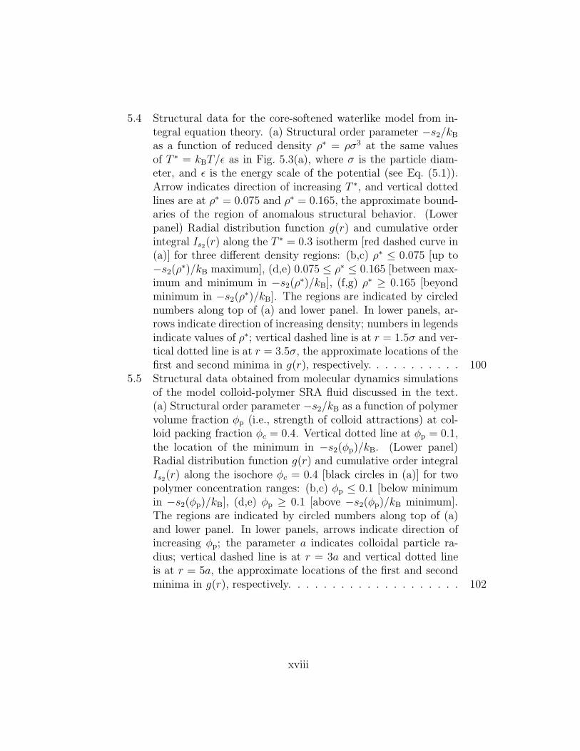
6.7 (Color online) Main panel: Shear viscosity versus order param-eter −s2 for the model colloid-polymer system. Arrow indicatesincreasing shear rate. Large filled symbols represent the data atzero shear. Symbols are the same as in Fig. 6.1. Lines are fitsof the nonequilibrium data to Eq. (6.6). Inset: Zero-shear vis-cosity obtained by equilibrium simulations versus that obtainedfrom extrapolation based on −s2 (see text). . . . . . . . . . . 124

6.8 (Color online) Main panel: Shear viscosity versus order param-eter −s2 of the Lennard-Jones fluid at several values of temper-ature T and packing fraction φc. Large filled circles representthe data at zero shear. Solid Lines are fits of the nonequilibriumdata to Eq. (6.6). Inset: Zero-shear viscosity obtained by equi-librium simulations versus those obtained from extrapolationbased on −s2 (see text). . . . . . . . . . . . . . . . . . . . . . 126

xx

7.1 (a) Natural and flat density profiles ρ(z), and (b) natural andstructured density profiles for a confined WCA fluid with aver-age density ρavg = 0.6 and H = 4, as discussed in the text. (c)The associated particle-boundary interactions φext(z). . . . . . 132

7.2 Effect of boundary interaction (shape of density profile) on (a)excess entropy per particle ∆sex(λ) = sex(λ) − sex(0) , (b) self-diffusivity D, and (c) viscosity η for the confined WCA fluidwith ρavg = 0.6 and H = 4. The centerline corresponds tothe fluid with the natural density profile of Fig. 1(a) and (b).From center to left, the density profile is systematically flat-tened: φ0(z) = λfφ0,f(z), where λf = 1 yields the flat profileshown in Fig. 1(a). From center to right, the density profile isstructured: φ0(z) = λsφ0,s(z), where λs = 1 produces the struc-tured profile shown in Fig. 1(b). Symbols are simulation data,and curves are guide to the eye. . . . . . . . . . . . . . . . . . 135

7.3 (a) Excess entropy per particle sex, (b) self-diffusivity D, and (c)viscosity η, of the confined WCA fluid versus average densityρavg at H = 4. Symbols are simulation data, and curves areguide to the eye. . . . . . . . . . . . . . . . . . . . . . . . . . 137

8.1 Mean-square displacement 〈δr2〉 of the small type 2 particlesversus time at packing fraction φc = 0.57 (black) and 0.582(red). Dashed lines are fits of 〈δr2〉 = 6Dt to the long timebehavior resulting in D = 1.2×10−3 and 1.5×10−4 at φc = 0.57and 0.582, respectively. . . . . . . . . . . . . . . . . . . . . . . 142

8.2 Distribution of the logarithm of squared displacements P [log10(δr2); τ ]

at several values of τ at packing fraction φc = 0.57 for the smalltype 2 particles. The numbers in the figure correspond to thevalue of τ for the curve of the same color. . . . . . . . . . . . 144

8.3 Distribution of the logarithm of squared displacements P [log10(δr2); τ ]

at several values of τ at packing fraction φc = 0.582 for the smalltype 2 particles. The numbers in the figure correspond to thevalue of τ for the curve of the same color. Vertical line is atδr2 = 0.56, the approximate dividing line between mobile andimmobile particles (see text). . . . . . . . . . . . . . . . . . . 145

xxi

8.4 Logarithm of squared displacements log10[δr2(τ)] versus struc-

tural order −s(2)2 (δr2; τ) for the various particle mobility classes

at several values of time interval τ at φc = 0.57. The numbersin the figure correspond to the value of τ for the curve of thesame color. The size of the symbols are proportional to thefraction of particles belonging to each mobility class. . . . . . 148

8.5 Logarithm of squared displacements log10[δr2(τ)] versus struc-

tural order −s(2)2 (δr2; τ) for the various particle mobility classes

at several values of time interval τ at φc = 0.582. The numbersin the figure correspond to the value of τ for the curve of thesame color. The size of the symbols are proportional to thefraction of particles belonging to each mobility class. Horizon-tal dashed line at δr2 = 0.56, the boundary between mobile andimmobile particles (see Fig. 8.3 and text). . . . . . . . . . . . 149

8.6 Schematic of structure of particles just before and just after ahop. . . . . . . . . . . . . . . . . . . . . . . . . . . . . . . . . 151

8.7 Number of nearest neighbors around the type 2 particles forvarious mobility classes and time windows, n

(2)tot(δr

2; τ), at (a)φc = 0.57 and (b) φc = 0.58. The symbols in (a) and (b) are thesame as those in Figs. 8.4 and 8.5, respectively. The size of thesymbols are proportional to the fraction of particles belongingto each mobility class. . . . . . . . . . . . . . . . . . . . . . . 153

xxii

Chapter 1

Introduction

The aim of this thesis is to investigate connections between structure and dy-

namics in complex fluid systems. The structural metrics used are the excess

entropy, a translational order parameter motivated by the two-body contri-

bution to the excess entropy, and the free volume. The dynamical properties

studied are the self-diffusivity and shear viscosity. The class of complex flu-

ids that we focus on comprises model suspensions of colloidal particles with

attractive interactions that are short-ranged relative to their diameter. Exam-

ples of such systems include colloids in solutions of non-adsorbing polymers,

globular proteins, and even micelles.

The utility of relationships between fluid structure and dynamics is

twofold. Since accurate theories for fluid structure are already relatively well

developed, such relationships can provide a means to “predict” dynamical

properties. Moreover, casting dynamical properties in terms of structural prop-

erties may clarify some of the outstanding questions regarding the mechanisms

of relaxation processes in fluids.

In this chapter we discuss two methods for relating dynamics to struc-

ture, both of which have proven useful for simple liquids. We then introduce

1

the specific model systems and questions we wish to investigate. We also give

a brief outline of the chapters to follow.

1.1 Relating dynamics to structure

It is physically intuitive that dynamical processes of fluids should be funda-

mentally related to the structural arrangements of their constituent particles.

The search for ways to make such relationships quantitative continues to be

an important aim in the study of condensed matter systems. In fact, since re-

liable molecular theories already exist for predicting the static structural and

thermodynamic (but not dynamic) properties of equilibrium fluids [1], the dis-

covery of new, general relationships between structure and dynamics provides

a valuable means for predicting fluid transport coefficients. Several empirical

expressions relating the mobility and the static structure of simple atomic and

molecular liquids have been proposed and tested. Here we focus on two such

relationships, based on free volume and local translational order, respectively.

1.1.1 Free Volume and dynamics

Different measures have been introduced over the years for characterizing the

“free” volume of liquids [2]. In a qualitative sense, however, these measures

all describe the local space available for motion of the particles. As one might

expect, compression of a fluid generally brings the particles closer together

(i.e., reduces the average free volume per particle) and, for most systems, also

2

reduces the particle mobility. Based on this type of physical picture, Doolittle

[3] introduced one of the first, and simplest, relationships between transport

properties and free volume of equilibrium atomic fluids:

D ∝ exp[−BD/〈vf〉], (1.1a)

and

η0 ∝ exp[Bη/〈vf〉], (1.1b)

where D is the self-diffusivity, η0 is the zero-shear viscosity, 〈vf〉 represents

an average free volume per particle, and BD and Bη are (positive) system

dependent parameters. Clearly, in this formulation, D and η0−1 are increas-

ing functions of 〈vf〉. While subsequent work has refined both the Doolittle

model (see Liu et al. [4] for a recent review) and the methods for computing

free volumes, the fundamental hypothesis that mobility is a monotonically in-

creasing function of the average free volume per particle has remained largely

unchanged.

1.1.2 Structural order and dynamics

A recent simulation study by Mittal et al. [5], motivated by earlier observations

by Rosenfeld [6, 7], demonstrates that the transport properties of a number

of different model fluids are also related in a simple way to a different static

quantity, the molar excess entropy sex. Specifically, the following relationship

was found to describe the effects of isochoric cooling on the self-diffusivity of

3

dense fluids, D ∝ exp[Bsex]. Here, B is a density-dependent, but temperature-

insensitive, parameter. To connect this relationship to the underlying fluid

structure, sex can be expressed as a sum over contributions from two-, three-

, and higher-body correlations [8]. Other recent simulation studies [9] have

shown that the parameter s2, which depends only on density and the pair-

correlation function g(r) —and which is equal to the two-body contribution to

the excess entropy for equilibrium fluids— can also be approximately related

to the transport properties of dense fluids via similar expressions, e.g.,

D ∝ exp[BD s2], (1.2a)

and

η0 ∝ exp[−Bη0s2], (1.2b)

where BD and Bη0are parameters which may depend on density, but not on

temperature. These relationships provide a simple and direct link between the

dynamical properties and the static pair correlations of equilibrium fluids.

1.2 Complex dynamic properties of fluids

The relationships between structure and dynamics of the previous section have

been applied successfully to a variety of simple (i.e., bulk atomic) liquids in

equilibrium. However, a wide array of fluids in science and technology have

properties different than these “simple” liquids. In such cases, can the rela-

tionships between structure and dynamics of the previous section be applied?

4

Answering this question for a particular class of complex systems is the goal of

this work. In this section, we introduce some of the rich dynamical phenomena

we wish to understand in terms of fluid structure.

1.2.1 Anomalous dynamics of short-ranged attractive

fluids and re-entrant glass transition

Colloidal fluids play a central role both in technology as well as in guiding

our understanding of condensed matter. Regarding the latter, suspensions of

colloids are interesting model systems because they can behave collectively in

ways that are similar to atomic and molecular simple liquids [1] while simulta-

neously being both large and slow enough to allow experimental measurements

of their real-space structure and dynamics.

One reason why colloidal suspensions and atomic fluids display some

macroscopic behaviors that are qualitatively similar is the similarity of their

interparticle interactions. In simple liquids, particle interactions are typically

composed of a strongly repulsive core and a longer-ranged van der Waals at-

traction. Because attractive forces are longer-ranged and relatively weak com-

pared to those associated with the repulsive core, the repulsive interactions

between particles dominate the fluid structure [10, 11]. For this reason, the

simplest model atomic fluid is one composed of hard spheres [1]. Since some

colloids can be made to interact essentially as hard spheres when suspended in

solvent, they also display many of the same properties as simple atomic and

molecular fluids.

5

Despite the similarities between the behaviors of colloidal, atomic, and

molecular fluids, there are also important differences [12, 13]. For example, the

effective interparticle attractions between colloids can be “tuned” to be short-

ranged relative to the particle diameter σ. This may be achieved by adding

small non-adsorbing polymer to a colloidal suspension inducing a “depletion”

attraction [14]. Depletion attractions between colloids have a range on the

order of the polymer radius of gyration, which can be made to be a few percent

of the colloidal particle diameter. This “short-ranged” attraction can strongly

impact fluid structure, in stark contrast to the dispersion attractions in atomic

and molecular systems that decay more gradually with interparticle separation

r, i.e., as (σ/r)−6.

Short-ranged attractive (SRA) interactions have nontrivial implications

for the dynamic behavior of colloidal suspensions. For instance, whereas cool-

ing or compression is the only route to glass formation of simple atomic liquids,

recent work [15, 16, 17, 18] has shown that colloidal systems with short-ranged

attractive (SRA) interactions can form glasses not only upon cooling, but also

upon heating.

The basic physics behind this unusual phenomena has been discussed

extensively by Sciortino [13]. A schematic of the behavior discussed below is

given in Fig. 1.1. Consider a fluid suspension consisting of hard sphere particles

with diameter σ. At a packing fraction φc ≈ 0.58, such a fluid forms a glass

(red line in Fig. 1.1). In this case, particles are hindered from moving due to

exclude volume interactions between neighboring particles, which effectively

6

Figure 1.1: Dynamical transitions for fluid composed of particles with short-ranged attractions. The glass lines separate the “liquid” regions from the“glass” regions. The vertical black dashed line represents the hard-sphereglass line. In the case of short-range attractive colloids [15, 16], the re-entrant(non-monotonic) shape of the glass line (solid red and blue lines) creates apocket of liquid states that are stabilized by the short-range attraction. Thelocation of the theoretical glass-glass transition line (thick blue line) and theproposed connection between the gel-line (at low volume fractions) and theattractive glass line (solid blue line) are also indicated. Equilibrium (andmetastable) coexistence curves between liquid and solid phases – which in thecase of attractive colloids are significantly different from the case of simplefluids with long-range attractions – are not shown. (Adapted from Ref. [13])

7

form “cages” surrounding each particle. Particles can only rattle within their

cages on experimental time scales. We term such a state as a hard-sphere or

“packing”-driven glass.

Now, consider what happens when, in addition to the hard-sphere re-

pulsion, a short-ranged attractive interaction is present. If the system is at

a high temperature (relative to the strength of the attraction), the attrac-

tions have virtually no effect, and the fluid particles behave like hard spheres.

Therefore, at high temperatures and high packing fractions, even this system

forms a hard-sphere glass. As the temperature is lowered, it has been hypoth-

esized [13] that the strong SRA interactions cause particles to cluster together.

This in turn shrinks the size of the confining cages, and simultaneously opens

transient channels in the fluid [13]. Particles can diffuse through these open

channels, and hence the glass melts into a fluid upon cooling (hatched region

in Fig. 1.1).

If the system is cooled further, however, the interparticle attractions

lead to long lived physical bonds between particles. Therefore, cooling even-

tually leads to the formation of a new arrested state (blue line in Fig. 1.1).

We term this latter state as an attractive or “bond”-driven glass.

Since the structural and mechanical properties of the packing and bond

driven glasses can be very different, there is broad interest in understanding

the properties of the precursor fluids from which they are formed. Clearly,

as either glass transition is approached, the particle mobility will decrease.

Therefore, for an SRA fluid which displays the re-entrant glass transition, the

8

Figure 1.2: Effect of increasing the polymer volume fraction ϕRpolymer on the

structural relaxation time τα at colloid volume fraction ϕcolloid = 0.67. Thevertical lines schematically indicate the transitions lines to the respective glassystates. (Adapted from [15])

9

fluid will also display anomalous dynamics. By this we mean that heating such

a fluid will, under some conditions, lead to a decrease in mobility as the pack-

ing driven glass is approached, which is anomalous when compared to what

happens in simple atomic liquids. This behavior has been observed experi-

mentally. For example, Eckert and Bartsch [15] observed similar trends in a

binary colloidal suspension. Small linear polymers were added which induced

short-ranged depletion attractions between the colloidal particles (the strength

of interparticle attraction increasing with the polymer concentration). In this

study, the structural relaxation time τα (which behaves similarly to the viscos-

ity of the fluid) was investigated as a function of the polymer concentration.

As shown in Fig. 1.2, increasing the polymer concentration first decreases, and

then eventually increases the relaxation time.

How, and if, the unusual properties of short-ranged attractive systems

connect to the underlying structural properties of the fluid is still an open

question. We address the dynamical properties of model short-ranged attrac-

tive fluids in terms of free-volume and structural order in Chapters 2 and 4,

respectively.

1.2.2 Fluids under shear

It is well established that shearing a fluid changes its dynamical properties.

While a variety of models relating structure to dynamics, like those discussed

in Section 1.1, have been proposed for equilibrium fluids, corresponding re-

lationships for nonequilibrium fluids have received much less attention. In

10

Chapter 4, we examine if the shear viscosity of a fluid under shear can be

related in a simple way to either its free volume or its structural order.

1.2.3 Confined fluids

Fluids confined to length scales on the order of the fluid particle diameters

are important in variety of sciences and technologies. Examples range from

fluid flow in cells to membrane separation to micro-fluidic devices. Confining

a fluid to such scales can have drastic effects on structure, thermodynamic,

and dynamic properties. However, recent work has shown that the resulting

dynamics of the confined fluid are related to excess entropy in much the same

way as for the bulk fluid [19, 20, 21].

This presents a possible means to modify the dynamics of a confined

fluid. By altering how particles interact with the confining boundary (for ex-

ample, by changing the chemistry of the boundary), the way in which particles

spontaneously arrange can be tuned. This, in turn, changes the excess entropy

as well as the dynamical properties of the confined fluid. We quantitatively

explore these ideas for a model system in Chapter 7.

1.2.4 Structure and heterogeneous dynamics

Fluids at high temperatures are dynamically homogeneous in the sense that

the distribution of single-particle displacements are uniform about the mean

for intermediate and long times. The dynamics of deeply supercooled fluids

by contrast are nonuniform. For example, for intermediate time scales, the

11

distribution of particle displacements is bimodal; i.e., there are “mobile” and

“immobile” sub-populations. In Chapter 8, we address whether such hetero-

geneous dynamics can be related to the structural order of the fluid.

1.3 Thesis organization

Chapter 2: Free Volumes and the anomalous self-diffusivity of at-

tractive colloids [22]

Free volume theories for the dynamics of dense fluids commonly as-

sume (i) that diffusivity increases with average free volume per particle and

(ii) that the size distribution of free volumes can be approximated by that of

an equivalent hard-sphere reference system. We use molecular simulations to

demonstrate that these assumptions break down when one considers concen-

trated suspensions of particles with short-range attractions. In these systems,

self-diffusivity shows non-monotonic dependencies on both average free volume

and the strength of the interparticle attraction. Moreover, when interparticle

attractions are strong, the shape of the free volume distribution is qualita-

tively different than that of the corresponding hard-sphere reference fluid. We

propose a conceptual revision to the traditional free volume perspective that

takes into account both the size distribution and the persistence time of the free

volumes, and we demonstrate that it can qualitatively capture the disparate

behaviors of a model fluid with short-range attractions and its hard-sphere

reference fluid.

Chapter 3: Free Volumes and the anomalous self-diffusivity of at-

12

tractive colloids [23]

We introduce and test via molecular simulation a simple model for pre-

dicting the manner in which interparticle interactions and thermodynamic

conditions impact the single-particle free-volume distributions of equilibrium

fluids. The model suggests a scaling relationship for the density-dependent

behavior of the hard-sphere system. It also predicts how the second virial

coefficients of fluids with short-range attractions affect their free-volume dis-

tributions.

Chapter 4: How short-range attractions impact the structural order,

self-diffusivity, and viscosity of a fluid [24]

We present molecular simulation data for viscosity, self-diffusivity, and

the local structural ordering of (i) a hard-sphere fluid and (ii) a square-well

fluid with short-range attractions. The latter fluid exhibits a region of dynamic

anomalies in its phase diagram, where its mobility increases upon isochoric

cooling, which is found to be a subset of a larger region of structural anomalies,

in which its pair correlations strengthen upon isochoric heating. This “cascade

of anomalies” qualitatively resembles that found in recent simulations of liquid

water. The results for the hard-sphere and square-well systems also show

that the breakdown of the Stokes-Einstein relation upon supercooling occurs

for conditions where viscosity and self-diffusivity develop different couplings

to the degree of pairwise structural ordering of the liquid. We discuss how

these couplings reflect dynamic heterogeneities. Finally, we note that the

simulation data suggests how repulsive and attractive glasses may generally

13

be characterized by two distinct levels of short-range structural order.

Chapter 5: Structural anomalies of fluids: Origins in second and

higher coordination shells [25]

Compressing or cooling a fluid typically enhances its static interparticle

correlations. However, there are notable exceptions. Isothermal compression

can reduce the translational order of fluids that exhibit anomalous waterlike

trends in their thermodynamic and transport properties, while isochoric cool-

ing (or strengthening of attractive interactions) can have a similar effect on

fluids of particles with short-range attractions. Recent simulation studies by

Yan et al. [26] on the former type of system and Krekelberg et al. [24] on

the latter provide examples where such structural anomalies can be related to

specific changes in second and more distant coordination shells of the radial

distribution function. Here, we confirm the generality of this microscopic pic-

ture through analysis, via molecular simulation and integral equation theory,

of coordination shell contributions to the two-body excess entropy for several

related model fluids which incorporate different levels of molecular resolution.

The results suggest that integral equation theory can be an effective and com-

putationally inexpensive tool for assessing, based on the pair potential alone,

whether new model systems are good candidates for exhibiting structural (and

hence thermodynamic and transport) anomalies.

Chapter 6: Relationship between shear viscosity and structure of a

model colloidal suspension [27, 28]

We use molecular dynamics simulations to investigate whether two dif-

14

ferent structural quantities, free volume per particle and a metric for local

translational order, can be related to the shear rate dependent viscosity of a

model colloidal fluid. Our results suggest that while the characteristic auto-

correlation time of the free volumes (a dynamic quantity) qualitatively tracks

the shear viscosity of the fluid, the shear-rate-dependent average free volume

(a static quantity) does not. On the other hand, the translational order metric

does appear to be strongly correlated to the shear viscosity over a wide range

of conditions.

Chapter 7: Tuning density profiles and mobility of inhomogeneous

fluids [29]

Density profiles are the most common measure of inhomogeneous struc-

ture in confined fluids, but their connection to transport coefficients is poorly

understood. We explore via simulation how tuning particle-wall interactions

to flatten or enhance the particle layering of a model confined fluid impacts

its self-diffusivity, viscosity, and entropy. Interestingly, interactions that elimi-

nate particle layering significantly reduce confined fluid mobility, whereas those

that enhance layering can have the opposite effect. Excess entropy helps to

understand and predict these trends.

Chapter 8: Structural and dynamic heterogeneities

An outstanding question regarding supercooled fluids is whether the

emergence of heterogeneous dynamics is accompanied by heterogeneous struc-

tural characteristics. Using molecular simulations, we show that the mobility

of particles is related in a simple way to the structure of the particles surround-

15

ing them. Specifically, particles require a critical amount of local disorder to

be mobile on intermediate time scales.

16

Chapter 2

Free Volumes and the anomalous

self-diffusivity of attractive colloids

2.1 Introduction

Colloidal materials play an important role in technological applications as well

as in guiding our fundamental understanding of condensed matter. A variety of

synthesis techniques have been developed to tune colloidal interactions, making

them model systems for studying the general properties of fluids, crystals,

and other self-assembled structures. Interestingly, the effective attractions

between colloids can be tailored to be “short-ranged” relative to both the

particle diameter and the average interparticle spacing in solution [12]. Since

this type of short-range attraction (SRA) strongly affects particle ordering, the

thermodynamics of SRA fluids cannot be accurately described by first-order

perturbation theories that assume local particle structuring is determined by

hard-sphere (HS) repulsions [30, 31].

As discussed in Section 1.2.1 SRA fluids also display dynamical behav-

iors not observed in simple liquids. One pronounced difference is the manner

17

in which self-diffusivity D depends on the ratio of the thermal energy scale

kBT to the characteristic interparticle attractive energy ǫ. Simple liquids lose

mobility if isochorically cooled, and they form a glassy state at sufficiently low

T if crystallization is successfully avoided. However, in SRA systems at high

volume fractions, D exhibits a maximum as a function of kBT/ǫ, reflecting a

pocket of fluid states on the phase diagram between an “attractive” glass at

low kBT/ǫ and a “repulsive” glass at high kBT/ǫ [15, 16, 17, 18, 32, 33]. The

mechanisms for the diffusivity maximum and the re-entrant glassy behavior

of SRA fluids are of great fundamental interest, and a basic understanding

of these phenomena seems necessary if SRA materials are to realize their full

potential in technological applications.

In this chapter, we use molecular dynamics (MD) simulations and statis-

tical geometry tools to compare the structural origins of the self-diffusivity for

two systems: a model SRA fluid and a HS reference fluid. In particular, we ex-

plore how their self-diffusivities relate to the properties of their single-particle

free volumes. We find that two common assumptions about free volumes and

dynamics of the liquid state (see [4] for a recent review), (i) that diffusivity

increases with increasing free volume and (ii) that the size distribution of free

volumes can be approximated by that of an equivalent HS reference system,

break down when one considers an SRA fluid. Therefore, we propose a concep-

tual revision to the traditional free volume perspective that takes into account

both the size distribution and the characteristic persistence time of the free

volumes. We demonstrate that this picture can qualitatively rationalize the

18

dynamical characteristics exhibited by these two important types of fluids.

2.2 Methods

2.2.1 Model fluid

The model SRA fluid that we examine was introduced by Puertas et al. [34, 35]

to qualitatively describe polymer-mediated depletion attractions in suspen-

sions of HS colloids. Its anomalous dynamical properties have now been

characterized extensively [36, 37, 38], and they typify those experimentally

observed in suspensions of SRA particles. The interparticle potential con-

sists of two main physical components: (i) a steeply repulsive (essentially HS)

contribution UHS(r12) = kBT (2a12/r12)36 (2a12 is the effective exclusion diam-

eter, and r12 is the center-to-center distance between particles 1 and 2) and

(ii) a polymer-induced depletion attraction UAO(r12) modeled by the Asakura-

Oosawa [39] potential. In the latter, the attractive strength increases with

the volume fraction of polymers in solution φp, while the range of attraction

is controlled by the radius of gyration of the polymers Rg, set in this case

to a/5, where a is the average particle radius. Following Puertas et al. [34],

we take the particle radii to be weakly polydisperse (drawn from a uniform

distribution with mean a and half-width ∆ = a/10) to prevent crystallization,

and we add a longer-range , soft repulsion UR to the interparticle potential to

prevent fluid-fluid phase separation. A complete discussion of the model SRA

fluid of Puertas et al. is presented elsewhere [35, 36, 38]. Figure 2.1 displays

19

the total colloidal potential USRA = UHS + UAO + UR for three different values

of φp.

2 3 4r/a

-4

0

4

8U

SR

A /

k BT

φp=0.00.20.4

φp

Figure 2.1: Effective colloidal pair potential of the model SRA fluid USRA(r)discussed in the text for various values of nonadsorbing polymer concentrationφp.

We also analyzed a reference fluid of particles that interact solely via

the HS component of the above SRA potential UHS(r12) = kBT (2a12/r12)36.

We refer to it as a HS reference fluid since, for the conditions analyzed here, its

properties are virtually indistinguishable from a fluid with a discontinuous HS

pair potential. We studied the SRA and HS reference fluids via MD simulations

in the microcanonical ensemble using N = 1000 particles and a periodically

replicated cubic simulation cell of volume V . The volume fraction of the

particles φc = 4Nπa3[1 + (∆/a)2]/3V was set for each simulation by choosing

V . The equations of motion were integrated using the velocity Verlet algorithm

[40] with a time step of 7.5 × 10−4a√

m/kBT , where m is particle mass. Self-

diffusivities D were calculated by fitting the long time (t ≫ 1) mean-squared

displacements to the Einstein relation for self-diffusivity 〈δr2〉 = 6Dt. From

20

here forward, we implicitly non-dimensionalize all quantities in this study by

appropriate combinations of the length scale a and the time scale a√

m/kBT .

2.2.2 Free volume

Figure 2.2: Two-dimensional schematic of particles (black circles) with exclu-sion disks (grey circles). The free volume of the shaded particle (left) is equalto the local connected volume of particle-center-accessible space that wouldbe formed if the particle were removed from the configuration (i.e., the cavityindicated by the hatched region, right).

To gain insights into the relationship between structure and dynamics in

the SRA and HS reference fluids, we studied how the self-diffusivities of these

systems relate to the static and dynamic properties of their free volumes. The

free volume of a single particle vf(t) was defined [41] to be the “cage” of con-

nected space that the particle center could geometrically access by translation

if every other particle in the system were held fixed in their positions at time

t (see Fig. 2.2). This definition assumes that steep interparticle repulsions

21

prevent particle centers from approaching closer than 2a12, the effective HS

particle diameter. We considered static quantities such as p(vf), the probabil-

ity density associated with an arbitrarily chosen particle having free volume vf ,

and the average free volume per particle 〈vf〉 ≡∫

yp(y)dy. We also considered

dynamic quantities such as the free-volume autocorrelation function Cvf:

Cvf(t) ≡

1

N

N∑

i=1

〈δvf,i(t)δvf,i(0)〉

〈δvf,i(0)δvf,i(0)〉, (2.1)

where δvf,i(t) = vf,i(t) − 〈vf,i(t)〉 is the deviation of particle i’s free volume

at time t from its average value. Cvf(t) characterizes the dynamic manner

in which the size of a particle’s free volume loses correlation with its initial

value due to thermal fluctuations. We calculated the free volumes from simu-

lated configurations of our model fluids using an exact analytical construction

presented earlier by Sastry et al. [11, 42] We neglect the weak polydispersity

in particle radii (i.e., we assume a12 = a) for the free volume analysis. This

allows us to use the Sastry et al. construction [11], which is formally exact for

monodisperse configurations of spherical particles.

2.3 Results and discussion

We begin by examining how the particle volume fraction φc affects the struc-

ture and dynamics of the HS reference fluid. Figures 2.3a and 2.3b display

the φc dependencies of self-diffusivity D and average free volumes 〈vf〉 respec-

tively. The monotonic decrease of both 〈vf〉 and D with increasing φc is in

22

0.3 0.4φc

0

1

2

D

0.3 0.4 0.5φc

0

1

2

0 0.5 1 1.5 2 2.5<vf>

0

1

2

3

D

(a) (b)

(c)

<vf >

Figure 2.3: HS reference fluid. (a) Self-diffusivity D versus particle volumefraction φc. (b) Average free volume 〈vf〉 versus particle volume fraction φc.(c) Self-diffusivity D versus average free volume 〈vf〉.

23

accord with the physically intuitive picture that, in the absence of strong at-

tractions that affect fluid structure, the local space accessible to the particles

controls their dynamics. Clearly, D and 〈vf〉 are positively correlated, as is

shown in Fig. 2.3c, which is consistent with the traditional free volume picture

for dynamics [4, 43]; A similar correlation can be expected to be found in

other molecular liquids with structures that can be adequately represented by

an athermal reference fluid.

Attractive interactions can, however, have a strong impact on the dy-

namics of an SRA fluid. For example, Fig. 2.4a illustrates that self-diffusivity

D for the Puertas et al. model displays a pronounced maximum with polymer

volume fraction φp (which governs the strength of interparticle attraction) for

φc = 0.4, 0.5, and 0.55. To explore whether this behavior is consistent with

a free volume based perspective for dynamics, we first show in Fig. 2.4b that

increasing φp from 0.1 to 0.4 increases the value of 〈vf〉 for the SRA fluid by

approximately an order of magnitude at each of the three values of φc ex-

amined here. In other words, the net affect of strengthening the short-range

attractions at constant φc is to increase the average local space available to

the particles.

One can understand the above trend in 〈vf〉 by considering how the

size distributions of the free volumes p(vf) are impacted by changes in φp at

constant φc (see Fig. 2.4c). At low φp, p(vf) is qualitatively similar to that

of the HS fluid [11]. However, as φp is increased, there are notable changes

in the populations of small, mid-sized, and large free volumes, giving p(vf)

24

0 0.2 0.4φp

10-3

10-2

10-1

D

0 0.2 0.4φp

10-2

10-1

100

<vf>

10-3

10-2

10-1 10

010

1

vf

10-4

10-2

100

P(vf)

HSφp=0.1

0.20.30.4

0.1 1<vf>

10-3

10-2

10-1

100D

(a) (b)

(c)

φc=0.4

(d)

Figure 2.4: SRA fluid (a) Self-diffusivity D versus polymer volume fraction φp.(b) Average free volume 〈vf〉 versus polymer volume fraction φp at particlevolume fractions φc = 0.4, 0.5, and 0.55. (c) Free volume size distributionp(vf) at φc = 0.4 for the HS reference fluid and the SRA fluid at (following thearrow) φp = 0.1, 0.2, 0.3, and 0.4. Dotted lines indicate boundaries of freevolume regions (see text). Qualitatively similar distributions occur for φc = 0.5and 0.55 (not shown) (d) Self-diffusivity D versus average free volume 〈vf〉 forthe HS reference fluid (open circles) and the SRA fluid at φc = 0.4 (closedcircles), φc = 0.5 (closed triangles), and φc = 0.55 (closed squares).

25

a shape that significantly departs from the HS behavior. Specifically, the

fraction of particles with small free volumes (vf < 10−2) or large free volume

(vf > 1) increases at the expense of the particles with mid-sized free volumes

(10−2 < vf < 1). This is a consequence of the known tendency of SRA particles

to cluster at high φp, a process that naturally creates transient “channels” of

void space believed to be crucial for understanding dynamic processes of the

fluid [36, 13]. Particles on the interior of clusters have small free volumes, while

those populating cluster surfaces near void channels have large free volumes.

The pronounced increase in 〈vf〉 with φp at high φp suggests that it is the

particles on the cluster surfaces that control the average free volume.

The data of Fig 2.4a and Fig 2.4b also demonstrate that D and 〈vf〉

can be negatively correlated for the SRA fluid (see Fig. 2.4d). This represents

a significant departure from the behaviors of the HS reference fluid and other

recently simulated liquids [43], as well as from what is qualitatively expected

based on free volume theories [4] for dynamics.

To fully understand the anomalous dynamics of the SRA fluid from a

free volume perspective, one must account for the fact that attractions actually

have two effects on the free volumes. First, as discussed above, attractions

increase the average local space available to the particles and render the free

volume distribution more inhomogenenous. These changes act to increase

the mobility of the fluid. However, strong attractions also have an effect on

dynamics: they cause the cages of free volume to become longer-lived, which

acts to slow down cooperative rearrangements and thus reduce single-particle

26

mobility. To quantify the trade-off between these two effects, we first need a

method for measuring the latter.

We probed the persistence of the free volume cages in the model HS

reference and SRA fluids by calculating the free volume autocorrelation func-

tion Cvf, defined in Eq. (2.1) (see Figs. 2.5a and 2.5b). In both systems, the

decorrelation of the free volume was observed to be consistent with a three-

part process, described qualitatively below. First, a small decorrelation was

observed at very short times, most likely due to inertial effects. The second

component, a slower process, can be ascribed to local vibrational motions of

neighboring particles that distort the free volume cage. The third and slowest

part of the decorrelation can be ascribed to larger collective particle rear-

rangements. To quantify these, we extracted characteristic time scales from

the autocorrelation functions. The inertial component was modeled as a Gaus-

sian and both the vibrational and collective rearrangement components were

modeled as exponential decays (see caption of Fig. 2.5). We expect the time

scale associated with collective rearrangements, which we refer to as the free

volume persistence time τf , to be the relevant one for self-diffusivity in dense

fluids.

Figures 2.5c and 2.5d show the behavior of τf for the HS reference and

SRA fluids, respectively. In the former, τf increases monontonically with φc,

reflecting the fact that packing frustration slows down the collective rearrange-

ments of the particles as density is increased. As expected, similar behavior

is observed for the φc dependence of τf in the SRA fluid at low polymer con-

27

10-1

101 10

30

0.2

0.4

0.6

0.8

1C

v f(t)

φc=0.40.450.50.550.57

10-1

101 10

3

φp=0.0

0.10.20.30.350.4

0.4 0.45 0.5 0.55φc

100

101

102

τ f

0 0.1 0.2 0.3φp

t

(a) (b)

(c) (d)

Figure 2.5: Free volume autocorrelation function Cvfversus time t for (a) the

HS reference fluid (arrow indicates increasing φc) and (b) the SRA fluid (arrowindicates increasing φp). Lower panel: free volume persistence times τf cal-culated by fitting Cvf

to the form Cvf(t) = Afe

−t/τf + Ave−t/τv + AGe

−(t/τG)2/2

(subscripts v and G denote the vibrational and Gaussian contributions, respec-tively) for (c) the HS reference fluid as a function of particle volume fraction φc

and (d) the SRA fluid as a function of polymer volume fraction φp at φc = 0.4(circles), φc = 0.5 (triangles), and φc = 0.55 (squares). For all cases studiedfor both models, τf was found to be larger than τv by an order of magnitudeor more.

28

centrations φp, where packing effects also dominate. At the lowest particle

volume fraction of φc = 0.40, we find that increasing interparticle attractions

(i.e, increasing φp) has little effect on the SRA fluid below φp ≈ 0.2. However,

increasing φp above 0.2 renders the interparticle bonds strong enough to slow

down the collective rearrangements of the particles, causing a pronounced rise

in τf .

The effect of short-range attractions on dynamics becomes far richer

at the higher particle packing fractions of φc = 0.5 and 0.55. Here, for poly-

mer volume fractions below φp ≈ 0.2, increasing φp significantly reduces the

characteristic time for collective particle rearrangements. This is because, as

was illustrated in Fig 2.4c and envisioned earlier by Sciortino [13], weak attrac-

tions make the free volume distribution more inhomogeneous, which eliminates

some of the packing inefficiencies of the dense repulsive fluid and allows for

greater average particle mobility. However, above φp ≈ 0.2, collective rear-

rangement again becomes slower with increasing φp, now due to the formation

of a progressively more attractive interparticle “bond” network.

As a final test of the relationship between free volumes and the anoma-

lous dynamical properties of the SRA fluid, we examine a simple relationship

motivated by the idea that D should scale like the square of a length relevant

for diffusion divided by a characteristic time. One reasonable choice for the

length scale in this picture is the free volume cage dimension 〈vf〉1/3. We found

that other obvious choices such as 〈v1/3f 〉 and

√

〈v2/3f 〉 produce similar results.

For an associated time scale, we use the persistence time of the free volumes

29

0 0.1 0.2 0.3φp

10-3

10-2

10-1

100

D

0.45 0.5 0.55φc

10-2

10-1

100

(a) (b)

Figure 2.6: Comparison of self-diffusivity D (closed symbols) to that estimated

using the relation D = C〈vf〉2/3/τf (open symbols) for (a) the SRA fluid as a

function of polymer volume fraction φp at particle volume fraction φc = 0.4(circles), φc = 0.5 (triangles), and φc = 0.55 (squares) and for (b) the HSreference fluid as a function of particle volume fraction φc. The parameter Cdoes not depend on φp or φc, and it was chosen for each model to provide areasonable overall fit to the simulation data.

30

τf . We then expect D ≈ C〈vf〉2/3/τf , where C is a system dependent constant.

In Fig. 2.6, we show that this type of simple relationship can qualitatively

capture the nontrivial φp and the φc dependencies of D for the SRA model,

as well as the qualitative behavior of the HS reference fluid.

2.4 Conclusions

We have shown via molecular simulation that SRA fluids expose some weak-

nesses in the ideas underlying traditional free volume theories for dynamics.

Although a formal theory is still lacking, we propose a conceptual revision to

those ideas that appears to reconcile the behavior of SRA fluids with a free

volume based perspective. The results of this study emphasize the impor-

tance of understanding both the size distribution and the dynamics of the free

volumes.

31

Chapter 3

Model for the free-volume

distributions of equilibrium fluids

3.1 Introduction

Liquid-state theory aims to provide a framework that links the interparticle

interactions of a fluid with its local structure, thermodynamic properties, and

transport coefficients. One of the central quantities for characterizing the

structural order is the static structure factor S(k) (or, equivalently, the pair

correlation function g(r)) [44]. The structure factor can be readily measured

by scattering experiments, computed via molecular simulations, or estimated

using integral equation theories. Thermodynamic properties of fluids with

pairwise interactions can be calculated directly from S(k) using exact rela-

tionships from statistical mechanics. Furthermore, many of the nontrivial dy-

namical behaviors of liquids can be predicted from a knowledge of S(k) using

mode-coupling theory and its recent extensions [44, 45, 46].

However, despite its considerable practical value, S(k) cannot provide a

comprehensive description of liquid structure mainly because it only contains

32

information about the spatial correlations between pairs of particles. Higher-

order correlation functions, or suitable approximations for them, are required

to predict structural quantities that depend on the relative positions of three or

more particles. A well known example of such a quantity is the single-particle

free volume vf , illustrated in Fig. 3.1. It is defined as the cage of accessible

volume that a given particle center could reach from its present state if its

neighboring particles were fixed in their current configuration [41]. Restated

in simple terms, vf quantifies the “breathing room” that a particle has in its

local packing environment. The thermodynamic properties of purely athermal

(i.e., hard-core) fluids can be formally related to the statistical geometry of

their single-particle free volumes [41, 47, 48, 11, 49].

The idea that relaxation processes should also be linked to free volumes

has a long history in studies of the liquid state [50, 51, 52]. and it has moti-

vated the development of numerous “free-volume based” models for predicting

transport coefficients [4]. As was shown in Chapter 2, static free volume it-

self may not correlate to dynamics for complex fluid systems. Despite this,

the results of Chapter 2 make it is clear that the distribution of free volumes

can provide new insights. Unfortunately, a general microscopic framework has

yet to emerge, in part due to the computational and experimental difficulties

associated with measuring and characterizing free volumes. However, recent

advances in computational statistical geometry [11, 42] have made it possible

to efficiently calculate such properties from particle configurations obtained via

either experiments (e.g., confocal microscopy of colloidal suspensions [53, 54])

33

or computer simulations [11, 55, 43, 22]. These methods have catalyzed new

efforts to quantitatively examine the basic ideas underlying the free-volume

perspective for dynamics and, hence, the prospects for developing a successful

microscopic theory.

In this chapter, we contribute to one aspect of this effort by introduc-

ing a simple model for predicting the statistical geometry of single-particle

free volumes in equilibrium fluids. We use the aforementioned computational

tools of statistical geometry to test the predictions of the model for (i) the

hard-sphere (HS) fluid and (ii) a fluid of particles with short-ranged, square-

well attractions. The former is the standard structural reference fluid for

simple liquids. The latter serves as an elementary model for the behavior of

suspensions of attractive colloids and globular proteins, whose structures can

be strongly influenced by interparticle attractions. As we show, our model

suggests a scaling relationship for the density-dependent behavior of the HS

system. It also predicts the manner in which the second virial coefficients of

fluids with short-range attractions affect their free-volume distributions.

3.2 General Framework

We consider a three-dimensional (3D) equilibrium fluid comprising N identical

spherical particles contained in a macroscopic volume V at temperature T .

The packing fraction is φc = Nπσ3/6V , where σ is the diameter of a particle,

and the particles interact via a short-range isotropic pair potential Vij(r) of

34

the generic form

Vij(r) =

∞ r < σ,

u(r) σ ≤ r < σ(1 + ∆),

0 r ≥ σ(1 + ∆),

(3.1)

where ∆ ≤ 1. If one chooses u(r) = −ǫ, then Eq. (3.1) describes a square-well

interaction. Alternatively, the hard-sphere potential is recovered if ∆ = 0. We

are interested in developing a general strategy for predicting how Vij(r), φc, and

T affect the statistical properties of the fluid’s single-particle free volumes. To

simplify notation, we implicitly non-dimensionalize all lengths from this point

forward by the hard-core diameter σ of the particles.

The problem described above cannot be treated exactly, and so we

make some simplifying approximations that we later assess by comparing our

predictions to results obtained via molecular simulations. Our basic working

assumption is that the statistical geometry of the free volumes in the 3D fluid

at T and φc can be predicted based on a knowledge of the exact free-volume

distribution f1D of the corresponding one-dimensional (1D) fluid at the same

temperature T and the scaled packing fraction ξ = φc/φc,MRJ. We choose

φc,MRJ = 0.64 to ensure that the close packing limit of the 1D fluid (ξ = 1)

maps onto the maximally random jammed state of the 3D system [56]. Our

specific idea is that a particle’s free volume in the 3D fluid at T and φc can

be modeled as a cuboid (see Fig. 3.1) with length αxf , height αyf , and width

αzf , where xf , yf , and zf are independent random variables drawn from f1D at

35

Figure 3.1: A 2D schematic of the free volume of a tagged particle. Overlap-ping grey circles represent the exclusion spheres of the neighboring particles.(a) The small dashed circle is the tagged particle surface, and the larger dashedcircle is its associated exclusion sphere. The cross-hatched region is the taggedparticle’s free volume. (b) An expanded view of the tagged particle’s free vol-ume along with its approximate representation in our model.

36

T and ξ. The 3D free-volume distribution f(vf) is thus

f(vf) =

∫ ∞

0

dx

∫ ∞

0

dy

∫ ∞

0

dz δ(vf − α3xyz)f1D(x)f1D(y)f1D(z). (3.2)

The constant α is a scale factor chosen to ensure that our construction ac-

curately reproduces the equilibrium free-volume distributions and thermody-

namic properties of the 3D HS fluid (discussed below). Also of interest is the

probability density ϕ(sf) associated with finding a 3D free volume with surface

area sf . Using our model, ϕ(sf) can be expressed as

ϕ(sf) =

∫ ∞

0

dx

∫ ∞

0

dy

∫ ∞

0

dz δ(sf − 2α2[xy + xz + yz])f1D(x)f1D(y)f1D(z). (3.3)

Eq. (3.2) and (3.3) indicate that, in order to predict f(vf) and ϕ(sf) using

our approach, one only needs to derive the state-dependent form of f1D from

knowledge of Vij(r). However, f1D is given by

f1D(xf) =

∫ ∞

0

dyL

∫ ∞

0

dyR δ(xf − yL − yR)pg(yL)pg(yR)dyLdyR, (3.4)

where pg(z) is the probability density associated with finding a gap of size

z between the surfaces of two neighboring particles in the corresponding 1D

fluid. For particles that interact via a pair potential of the form given by

Eq. (3.1), Gursey[57] has shown that pg(z) can be written

pg(z) =e−βΠ[z+1]e−βVij(z+1)

∫ ∞0e−βΠ[s+1]e−βVij(s+1)ds

, (3.5)

37

where β = (kBT )−1, and Π is the 1D pressure. The equation of state of the

1D fluid, i.e., the dependence of Π on β and ξ, can be found implicitly from

the following relation [57]:

βξ−1 = −

(

∂ lnψ

∂Π

)

T

, (3.6)

where

ψ =

∫ ∞

0

dx e−βΠxe−βVij(x). (3.7)

Having outlined the general strategy of our model, we examine some of

its predictions for two specific systems in Section 3.3: (i) the equilibrium HS

fluid and (ii) an equilibrium square-well fluid with short-range attractions.

3.3 Testing the model

3.3.1 Predictions for the HS fluid

Here we apply the model of Section 3.2 to predict the statistical geometry of

the free volumes in the equilibrium HS fluid, where the pair potential Vij(r) is

given by

Vij(r) =

∞ r < 1,

0 r ≥ 1.

(3.8)

From Eq. (3.8), (3.6), and (3.7), it follows that the equation of state of the 1D

HS fluid is given by [58]

βΠ/ξ = 1/(1 − ξ). (3.9)

38

Substituting Eq. (3.9) and (3.8) into Eq. (3.5), yields the corresponding gap-

size distribution,

pg(z) =ξ

1 − ξe−zξ/(1−ξ). (3.10)

Then, from Eq. (3.4), f1D(xf) is simply

f1D(xf) = xf

(

ξ

1 − ξ

)2

e−xfξ/(1−ξ). (3.11)

The first moment of this distribution is

〈xf〉 ≡

∫ ∞

0

dxf xff1D(xf) =2(1 − ξ)

ξ. (3.12)

Defining x∗f ≡ xf/〈xf〉, we have

f1D(xf)dxf = f ∗1D(x∗f )dx

∗f , (3.13)

where

f ∗1D(x∗f ) = 4x∗f e

−2x∗f . (3.14)

The main implication is that while f1D is a function of xf and the packing

fraction ξ for the 1D HS fluid, f ∗1D(x∗f ) can be represented by a single curve

that is independent of ξ. As we show below, this property, when used in

combination with Eq. (3.2) and (3.3) of our model, leads to scaling predictions

for the density-dependent free-volume and free-surface distributions of the 3D

HS fluid.

39

In particular, making use of Eq. (3.2), (3.11), and (3.12), we identify

that

〈vf〉 ≡

∫ ∞

0

dv vf(v) = α3〈xf〉3 = 8α3

(

1 − ξ

ξ

)3

. (3.15)

Similarly, combining Eq. (3.3), (3.11), and (3.12) yields

〈sf〉 ≡

∫ ∞

0

ds sϕ(s) = 6α2〈xf〉2 = 24α2

(

1 − ξ

ξ

)2

. (3.16)

Now, if we normalize the 3D free volume by its first moment, v∗f ≡ vf/〈vf〉,

then we have

f(vf)dvf = f ∗(v∗f )dv∗f , (3.17)

where

f ∗(v∗f ) =

∫ ∞

0

dx

∫ ∞

0

dy

∫ ∞

0

dz δ(v∗f − xyz)f ∗1D(x)f ∗

1D(y)f ∗1D(z). (3.18)

Similarly, if we introduce the reduced free surface s∗f ≡ sf/〈sf〉, then it follows

that

ϕ(sf)dsf = ϕ∗(s∗f )ds∗f , (3.19)

where

ϕ∗(s∗f ) =

∫ ∞

0

dx

∫ ∞

0

dy

∫ ∞

0

dz δ(s∗f − [xy + xz + yz]/3)f ∗1D(x)f ∗

1D(y)f ∗1D(z). (3.20)

Eq. (3.18) and (3.20), when viewed together with Eq. (3.14), show that our

model predicts that the scaled free-volume and free-surface distributions, f ∗(v∗f )

40

and ϕ∗(s∗f ), are independent of packing fraction for the 3D HS fluid. We will

return to this point later, when we test the predictions of the model via molec-

ular simulations.

To use the model to predict the shapes of the free volumes in the 3D

HS fluid, we analyze the behavior of the dimensionless sphericity parameter

λf , defined as [59, 60]

λf = sf(6π1/2vf)

−2/3. (3.21)

The sphericity parameter takes on its minimum possible value (λf = 1) for

a spherical free volume, while it is larger in magnitude for less symmetric

free volumes. Our model predicts that the average value of the sphericity

parameter (quantifying the average shape of the free volumes), given by

〈λf〉 =

∫ ∞

0

dx

∫ ∞

0

dy

∫ ∞

0

dz2(xy + xz + yz)

(6π1/2xyz)2/3f1D(x)f1D(y)f1D(z) ≃ 1.57, (3.22)

is independent of packing fraction for the 3D HS fluid.

Finally, the equation of state of the 3D HS fluid can be formally related

to the statistical geometry of its free volumes [41, 47, 11]:

βP

ρ= 1 +

1

6

⟨

sf

vf

⟩

. (3.23)

Here, P is the pressure of the 3D fluid, and ρ = N/V is its number density.

41

In our model, it is easily shown that

⟨

sf

vf

⟩

=

∫ ∞

0

dx

∫ ∞

0

dy

∫ ∞

0

dz2(xy + xz + yz)

αxyzf1D(x)f1D(y)f1D(z) =

6α−1ξ

1 − ξ,

(3.24)

and therefore we have

βP

ρ=

1 − (1 − α−1)ξ

1 − ξ. (3.25)

3.3.2 Simulations of the HS Fluid

To test the predictions of our free-volume model for the 3D equilibrium HS

fluid, we have performed a series of molecular dynamics simulations using a

standard event-driven algorithm [61]. All runs were carried out in the mi-

crocanonical ensemble using N = 1000 particles and a periodically-replicated

cubic simulation cell. Snapshots of the system’s equilibrium configurations

were collected and used to calculate the geometric properties of single-particle

free volumes via the exact algorithm presented by Sastry et al. [11, 42] (see

Section 2.2.2).

Numerical predictions using the free-volume model introduced here re-

quire specifying the value of the geometric scale factor α shown in Fig. 3.1.

As discussed in Section 3.2 , the goal is to choose α in a way that allows the

model to provide a reasonable overall description of the statistical geometry,

and hence the thermodynamic properties, of the HS fluid. Throughout this

work we set α = 0.29, which we obtained from a least-squares fit of Eq. (3.15)

to the HS simulation data for 〈vf〉 versus φc over the range 0.375 ≤ φc ≤ 0.525.

42

The quality of this fit is illustrated in the inset of Fig. 3.2a.

We also compare in Fig. 3.2a the free-volume distributions f(vf) ob-

tained from simulations with those predicted via Eq. (3.2). We observe that

the model describes the data relatively well, with the predictions becoming

semi-quantitative for the higher packing fractions investigated. This trend

with packing fraction is expected since the simulated free volumes become

more compact at higher densities, and, as a result, they more closely resemble

the simple cuboid shapes that we have assumed in our model.

The same free-volume distributions shown in Fig. 3.2a are also shown

in Fig. 3.2b, only now scaled in the manner suggested by Eq. (3.18). This

rescaling yields the probability density associated with observing a particle

with a particular value of v∗f = vf/〈vf〉. Interestingly, we observe that, to a

very good approximation, the scaled distributions obtained via simulation for

all packing fractions investigated collapse onto a single curve predicted by the

model.

As can be seen by Eq. (3.20), the model predicts that the distributions

of free surfaces for the HS fluid should also collapse onto a single curve when

scaled in an analogous way. We compare in Fig. 3.3a the scaled free-surface

distributions ϕ∗(s∗f ) obtained via simulation to the predictions of Eq. (3.20).

Again, the collapse of the simulation data is striking, and it is described rea-

sonably well by the free-volume model. The inset of Fig. 3.3a compares the

average free-surface area per particle 〈sf〉 obtained from simulations to the

prediction of Eq. (3.16). As with the predictions for f(vf), the model provides

43

10-4

10-3

10-2

10-1

100

vf

10-3

10-1

101

103

f (v f)

10-2

10-1 10

010

1

vf*

10-5

10-3

10-1

101

f *(v

f*)

0.4 0.5φc

0

0.03

0.06

<vf>

φc

(a)

(b)

Figure 3.2: (a) Free-volume distributions of the 3D HS fluid for packing frac-tions φc = 0.375, 0.4, 0.425, 0.45, 0.475, 0.5 and 0.525. Symbols are simulationdata and solid curves are the predictions of Eq. (3.2). The arrow indicates in-creasing packing fraction φc. Inset: Average free volume 〈vf〉 versus packingfraction φc. Circles are simulation data and the solid line is the prediction ofEq. (3.15). (b) Probability density associated with observing particles withscaled free volume v∗f = vf/〈vf〉. Symbols are simulation data from panel (a)and the solid line is the prediction of Eq. (3.18).

44

10-2

10-1 10

010

1

sf*10

-4

10-3

10-2

10-1

100

ϕ∗(s

f*)

0.4 0.5φc

1

1.5

2

<λf>

0.4 0.5φc

0

0.5

1

1.5<s

f>

(a)

(b)

Figure 3.3: (a) Proabability density associated with observing particles withscaled free surface area s∗f = sf/〈sf〉 in the 3D HS fluid for packing fractionsφc = 0.375, 0.4, 0.425, 0.45, 0.475, 0.49, 0.5, 0.51, and 0.525. Symbols are sim-ulation data and solid curves are the predictions of Eq. (3.20). Inset: Averagefree surface area 〈sf〉 versus packing fraction φc. Circles are simulation dataand the solid line is the prediction of Eq. (3.16). (b) Average sphericity 〈λf〉 offree volumes in the HS fluid versus packing fraction φc. Circles are simulationdata, and the solid line is the prediction of Eq. (3.22).

45

a more accurate description of 〈sf〉 at higher packing fractions where the free

volumes are expected to be more compact. At low packing fractions, particles

will on average have more nearest neighbors which define their free-volume

then at high packing . Therefore, we expect our cuboid approximation to

break down at low packing fractions.

To quantify the compactness of the HS free volumes, we compare in

Fig. 3.3b the average sphericity of the free volumes 〈λf〉 calculated from the

simulations to that predicted by Eq. (3.22). We find that while the cuboid

representation of free volumes in our model underestimates 〈λf〉, it qualita-

tively captures the fact that, on average, the shapes of the free volumes in the

HS fluid are fairly insensitive to changes in packing fraction.

Finally, we test the ability of our free-volume model to predict the

equation of state of the HS system. In particular, we compare Eq. (3.25) to

the well-known Carnahan-Starling [62] equation, which provides an accurate

description of the HS pressure for packing fractions in the equilibrium fluid

range 0 < φc < 0.494. As can be seen in Fig. 3.4, Eq. (3.25) shows good

agreement with the Carnahan-Starling equation for the equilibrium HS fluid.

Moreover, while the Carnahan-Starling equation diverges at the unphysically

high packing fraction of φc = 1, Eq. (3.25) predicts that the HS fluid becomes

incompressible at the packing fraction of the maximally random jammed state

(φc,MRJ = 0.64) [56].

46

0 0.1 0.2 0.3 0.4 0.5φc

0

5

10

15

βP/ρ

−1

Statistical Geom.Carnahan-Starling

0.2 0.4 0.6 0.8 1φc

101

103

105

βP/ρ

−1

Figure 3.4: Equation of state for the HS fluid as calculated from both Eq. (3.25)and the Carnahan-Starling [62] relationship. Inset: Expanded version illus-trating that Eq. (3.25) diverges at φc,MRJ = 0.64, while the Carnahan-Starlingrelationship diverges at the unphysically high packing fraction of φc = 1.

47

3.3.3 Predictions for the Square-Well Fluid

To demonstrate that the ideas outlined in Section 3.2 can be readily extended

to other fluid systems, we now use our approach to predict the free-volume

distributions of a square-well fluid with short-range attractions, a basic model

system for suspensions of attractive colloids and globular proteins. Fluids with

short-ranged attraction are of particular interest here because, as shown in

Chapter 2, they exhibit free-volume distributions with shapes that differ from

that of the equilbrium HS fluid at the same packing fraction [22]. Specifically,

interparticle clustering induced by the short-range attractions increases the

populations of both large and small free volumes at the expense of mid-sized

free volumes. As discussed in Chapter 2, these structural changes play an

important role in the anomalous dynamical properties exhibited by these fluids

[22], and the ability to predict such changes constitutes a sensitive test of our

free-volume model.

The square-well pair potential is given by

Vij(r) =

∞ r < 1,

−ǫ 1 ≤ r < 1 + ∆,

0 r ≥ 1 + ∆.

(3.26)

Using Eq. (3.26), (3.6), and (3.7), one can show that the equation of state of

48

the 1D square-well fluid can be expressed as

ξ−1 = 1 +1

βΠ+

∆e−βΠ∆(1 − e−βǫ)

1 − e−βΠ∆(1 − e−βǫ). (3.27)

Furthermore, by substituting Eq. (3.5), (3.26), and (3.27) into Eq. (3.4), one

finds that the corresponding 1D free-volume distribution is given by

f1D(xf)

Θ(xf)=

xf xf < ∆,

2e−βǫ(xf − ∆) − xf + 2∆ xf ∈ [∆, 2∆),

xfe−2βǫ + 2∆e−βǫ(1 − e−βǫ) xf ≥ 2∆,

(3.28)

where

Θ(xf) = e−βΠxf

[

βΠ

1 − e−βΠ∆(1 − e−βǫ)

]2

. (3.29)

By substituting Eq. (3.28) into Eq. (3.2), one can readily calculate the free-

volume distribution for the 3D square-well fluid numerically.

3.3.4 Simulations of the Square-Well Fluid

To test the theoretical predictions of our model for the 3D square-well fluid, we

have performed a series of event-driven molecular dynamics simulations [61]

using N = 1000 particles. As with the HS simulations described earlier, a cubic

simulation cell was employed with periodic boundary conditions. Equilibrium

configurations were stored during these runs and later used to calculate [11, 42]

the geometric properties of the single-particle free volumes. For all simulations,

49

the range of the square-well attraction was set to ∆ = 0.03. We studied

the fluid at packing fraction φc = 0.5 and 0.58. For the φc = 0.58 case, a

flat distribution of particles sizes with mean σ and half width δ = σ/10 was

used to prevent crystallization. We examined the behavior of the fluid for

various values of the strength of the interparticle attraction ǫ, which is often

quantified using the reduced second virial coefficient B∗2 = B2/B

HS2 . Here,

B2 = (1/2)∫

dr[1− exp(−βVij(|r|))] is the second virial coefficient of the fluid

of interest, and BHS2 = 2π/3 is that of the hard-sphere fluid. For the 3D

square-well fluid, B∗2 is given by

B∗2 = 3

∫ ∞

0

r2[1 − e−βVij(r)]dr

= 1 + (1 − eβǫ)[(1 + ∆)3 − 1].

(3.30)

The simulated results for the free-volume distributions are displayed in

Fig. 3.5a and 3.5b for φc = 0.5 and 0.58, respectively. As has been observed for

other model fluids with short-range attractions [22] (see Chapter 2), decreasing

B∗2 (increasing attractions) increases the populations of both large and small

free volumes at the expense of the mid-sized free volumes. These trends are

captured by the predictions of the free-volume model (Fig. 3.5b and 3.5d) using

Eq. (3.2), (3.28), and (3.29). It is evident that the model does not match the

simulation results as well at φc = 0.58 as at φc = 0.5. This is most likely due to

the 1D equation of state used in the model being less accurate at high packing

fractions. Although the free-volume model presented here does not reproduce

the square-well distributions with quanitative accuracy, it clearly captures the

50

10-2

100

102

f (v f)

10-4 10

-310

-210

-1 100

vf

10-2

100

102

10-2

100

102

104

f (v f)

10-4 10

-310

-210

-1

vf

10-2

100

102

104

(a)

(b)

B2*

B2*

B2*

B2*

(c)

(d)

φc=0.5Simulation

φc=0.5Model

φc=0.58Simulation

φc=0.58Model

Figure 3.5: Free-volume distributions for the square-well fluid at range ofattraction ∆ = 0.03, and reduced second virial coefficients B∗

2 = −0.04, 0.41,0.60, 0.78, 0.84, 0.91 and 0.94. (a) Simulations at packing fraction φc = 0.5 and(b) the free-volume model at described in the text at φc = 0.5. (c) Simulationsat packing fraction φc = 0.58 and (d) free-volume model at φc = 0.58. Arrowsindicate increasing B∗

2 .

51

important physical trends. Moreover, its predictions show surprisingly good

agreement with the simulation data, given that there are no free parameters

in the theory that are fit to data for the square-well fluid.

3.4 Conclusions

In summary, we have introduced a simple model for predicting the free-volume

distributions of equilibrium fluids, and we have tested this model using molecu-

lar simulations. The model suggests a new scaling for the density-dependencies

of the free-volume and free-surface distributions of the HS fluid, and these scal-

ings show very good agreement with simulation results. The free-volume model

also predicts a reasonably accurate hard-sphere equation of state in which the

pressure diverges at a packing fraction of φc = 0.64. Finally, the model pre-

dicts semi-quantitatively the manner in which the attractive strength affects

the free-volume distributions of a square-well fluid with short-range attrac-

tions. These considerations suggest that the free-volume model proposed here

can perhaps be used fruitfully within the free-volume based theories for dy-

namics of fluids to understand how their transport coefficients derive from

their microscopic interactions and thermodynamic conditions.

52

Chapter 4

How short-range attractions impact

the structural order, self-diffusivity,

and viscosity of a fluid

4.1 Introduction

Colloidal fluids play a central role both in technology and in the study of

condensed matter. Regarding the latter, suspensions of colloids are interesting

model systems because they can behave collectively in ways that are similar to

atomic and molecular liquids while simultaneously being both large and slow

enough to allow experimental measurements of their real-space structure and

dynamics. Despite the similarities between the behaviors of colloids, atoms,

and molecules, there also are important, qualitative differences [12, 13]. For

example, the effective interparticle attractions between colloids can be “tuned”

to be short-ranged relative to the particle diameter σ, unlike the dispersion

attractions in atomic and molecular systems that decay more gradually with

interparticle separation r, i.e., as (σ/r)−6.

As stated in Section 1.2.1, short-ranged attractive (SRA) interactions

53

have nontrivial implications for the static structural, equilibrium thermody-

namic, and dynamic behaviors of colloidal suspensions. For instance, whereas

cooling a simple atomic liquid generally slows down its dynamic processes,

several recent studies have demonstrated that reducing the temperature (or in-

creasing the attractive interactions) of an SRA fluid can have a non-monotonic

effect on its mobility. In fact, concentrated SRA fluids can vitrify not only upon

cooling, forming an “attractive” glass or gel, but also upon heating, forming

a “repulsive” or hard-sphere (HS) glass [15, 16, 17, 18, 32, 33, 13]. Since the

structural and mechanical properties of these glassy states can be quite differ-

ent, there is a broad interest in understanding the properties of the precursor

supercooled fluids from which they are formed.

In this chapter, we explore whether the unusual effect that temperature

has on the dynamics of SRA fluids reflects a more general connection between

the static structure and the dynamics of condensed phases. In doing so, we

find it instructive to view the behavior of SRA fluids in the context of another

well-studied system with anomalous dynamical trends, liquid water. Cold

water behaves differently than simple fluids in that its mobility increases upon

isothermal compression over a broad range of conditions. Interestingly, the

state points where water shows this behavior is a subset of a larger region

on its phase diagram where its local structural order anomalously decreases

upon compression [63, 64]. In other words, there is a “cascade of anomalies”

[63] where the pressure-induced disordering of liquid water emerges at a lower

density, and ultimately disappears at a higher density, when compared to

54

the pressure-induced increase in its mobility. It has been recently argued

[9, 65, 66] that this behavior follows from the fact that water approximately

obeys a scaling relationship between its self-diffusivity and the structural order

parameter −s2/kB, where s2 is the contribution to the fluid’s excess entropy

due to its static oxygen-oxygen pair correlations, and kB is the Boltzmann

constant.

Here, we use molecular dynamics simulations to systematically investi-

gate the relationships between static structural order (−s2/kB), self-diffusivity

(D), and viscosity (η) for both a HS fluid and an SRA fluid. One of our main

aims is to understand whether the latter shows a cascade of anomalies similar

to that of liquid water. Specifically, we are interested in whether the region on

the phase diagram of an SRA fluid where it becomes more mobile (higher D,

lower η) upon cooling is a subset of a larger set of conditions where the fluid

becomes more ordered (higher −s2/kB) upon heating. A second, and related,

goal of this study is to explore whether the relationships between D, η, and

−s2/kB can provide generic insights into the breakdown of the Stokes-Einstein

(SE) relation (Dη/T ≈ constant) in deeply supercooled liquids and also into

the structural properties of repulsive and attractive glasses.

In Section 4.2, we describe the two model systems examined in this

study and also the simulation methods used to carry out the investigation.

Then, in Section 4.3, we present our simulation results and discuss their rele-

vance for understanding the connection between structural order and mobility

in HS and SRA fluids. Finally, in Section 4.4, we present some concluding

55

remarks.

4.2 Modeling and Simulation

We focus on two model systems: a fluid of HS particles and a fluid of square-

well particles with short-range attractions, the latter of which we denote the

SW-SRA fluid. The interparticle potential V(r12) between particles 1 and 2

for these systems is given by

V(r12) =

∞ r12 ≤ σ12,

−ǫ σ12 < r12 < λσ12,

0 r12 ≥ λσ12.

(4.1)

where r12 is the distance between the particle centers, σ12 = (σ1 + σ2)/2 is

the interparticle diameter, and the parameters ǫ and λ set the magnitude

and range of the interparticle attraction, respectively. For the HS fluid, one

has λ = 1, and thus there are no interparticle attractions. We choose λ =

1.03 for the SW-SRA fluid, a range similar to that of other SW-SRA fluids

known to exhibit anomalous dynamical behavior [67, 33]. In order to avoid

crystallization in our study, and thus allow study of the supercooled fluid

states, we have drawn the individual particle diameters σi of both systems

from a Gaussian distribution with an average of σ and standard deviation of

s = 0.1σ. For practical reasons, we truncated this distribution so that all

particle diameters lie in the range σ − 3s ≤ σi ≤ σ + 3s. We have implicitly

56

non-dimensionalized all reported quantities in this investigation by appropriate

combinations of the characteristic length scale, lc = σ and a model-dependent

time scale τc. For the HS fluid, the characteristic time scale τc is cast in terms

of the temperature τc =√

mσ2/kBT , where m is the particle mass, while

for the SW-SRA fluid it is defined in terms of the attractive strength of the

potential, τc =√

mσ2/ǫ.

To explore the behavior of these model systems, molecular dynamics

simulations were performed using an event-driven algorithm [61] in the mi-

crocanonical ensemble. For all runs, N = 1000 particles were simulated in a

cubic simulation cell of volume V with periodic boundary conditions. Particle

packing fractions φc = π∑

σ3i /(6V ) in the range 0.35 ≤ φc ≤ 0.6 were investi-

gated for both model systems, and temperatures T in the range 0.3 ≤ T ≤ 2.0

were examined for the SW-SRA fluid. For each thermodynamic state point,

between three and ten independent simulations were performed in order to

estimate the errors in the transport coefficients. Self-diffusivities D were cal-

culated by fitting the long time (t ≫ 1) mean-squared displacements to the

Einstein relation for self-diffusivity 〈δr2〉 = 6Dt. Zero-shear viscosities were

calculated using the impulse limit of the Einstein formula [68]. The structural

order parameter −s2 was computed using the expression

−s2 =ρ

2

∫

{g(r)lng(r) − [g(r) − 1]}dr, (4.2)

where ρ = N/V is the number density, and g(r) is the average pair correlation

function. Note that −s2 = 0 for an ideal gas, and −s2 → ∞ for a perfect

57

crystalline lattice. Thus, as has been discussed at length elsewhere [69, 9, 65],

one can view −s2 as a scalar measure of the amount of pair-wise translational

order of the system.

4.3 Results and Discussion

4.3.1 Transport and Structural Properties

We now examine some of the state-dependent transport and structural prop-

erties of the HS and SW-SRA fluids. For the HS fluid, the quantities D, η,

and −s2 (non-dimensionalized as outlined in Section 4.2) depend only on the

packing fraction φc, whereas the corresponding dimensionless properties for

the SW-SRA fluid depend on both packing fraction φc and temperature T .

The transport properties of the HS fluid are displayed in Fig. 4.1. As

expected, with increasing packing fraction φc, the self-diffusivity D monotoni-

cally decreases, while the viscosity η monotonically increases. The changes in

both of these properties become more pronounced for φc > 0.55, conditions for

which D(φc) can be accurately fitted using either Vogel-Fulcher or power-law

functional forms [70] with a predicted divergence near φc ∼ 0.6.

Figure 4.1(c) illustrates that the SE relation in the slip limit, Dη ≈

(2π)−1, is approximately obeyed by this HS fluid for φc < 0.55. However, for

higher packing fractions, large positive deviations from the slip limit of the

SE relation become apparent [70]. This type of SE “breakdown” has been

observed in studies of several glass-forming fluids in their deeply supercooled

58

10-5

10-3

10-1

D

100

102

104

η

0.35 0.4 0.45 0.5 0.55φc

10-1

100

Dη

(a)

(b)

(c)

Figure 4.1: Transport properties of the HS fluid described in the text as afunction of packing fraction φc: (a) self-diffusivity D, (b) viscosity η, and (c)SE relationship Dη/T . The horizontal dashed line in (c) indicates (2π)−1,the expected value of the SE relation in the slip limit, and the vertical linedenotes the point at which which Dη = 1.2/(2π). In this work, we use thissimple heuristic to identify the breakdown of the SE relation.

59

states [71, 72, 73, 74].

We note that, as observed by previous investigators [70], the SE rela-

tion is not strictly obeyed by the HS fluid even at lower packing fractions. For

example, the product Dη varies by approximately 30% as the packing frac-

tion is increased from φc = 0.35 to 0.55. However, the breakdown of the SE

relation is typically understood to occur when the product begins to exhibit

a pronounced positive deviation from the slip value. In this work, we identify

the breakdown of the SE relation by the heuristic criterion, Dη ≥ 1.2/(2π).

As can be seen from Figure 4.1(c), this threshold is crossed at φc ≈ 0.55 for

the HS fluid investigated here.

The simulated transport properties of the SW-SRA fluid are displayed

in Fig. 4.2 as a function of reciprocal temperature T−1 along isochores. The

most striking feature of this plot is that D exhibits a maxima with inverse

temperature, a behavior that has also been observed in both experiments and

computer simulations of other SRA fluids [15, 16, 17, 18, 32, 33, 35, 34, 36]

and also observed in Section 2.3. As discussed in Section 1.2.1, this trend

becomes pronounced at high φc, where the system can ultimately form either

a repulsive glass by isochoric heating or an attractive glass or gel via isochoric

cooling.

The behavior of the zero-shear viscosity η of the SW-SRA fluid, dis-

played in Fig. 4.2(b), qualitatively mirrors that of its self-diffusivity. For a

more quantitative comparison, the SE relationship Dη/T is plotted in Fig-

ure 4.2(c). Note that the slip limit of the SE relation is again approximately

60

10-5

10-3

10-1

D

100

102

104

η

0.580.590.6

0.5 1 1.5 2 2.5 3 3.5T

-1

0

1

2

Dη/

T

φc=0.40.50.550.565

(a)

(b)

(c)

Figure 4.2: Transport properties of the SW-SRA fluid described in the textas a function of packing fraction φc and reciprocal temperature T−1: (a) self-diffusivity D, (b) viscosity η, and (c) SE relationship Dη/T . The horizontaldashed line in (c) indicates (2π)−1, the expected value of the SE relation inthe slip limit.

61

obeyed for the SW-SRA fluid over a broad range of T−1 and φc. However, for

all values of φc investigated here, the SE relation breaks down at sufficiently

low T , as the attractive glass transition is approached. At high T , on the other

hand, only the highest φc isochore studied showed a significant breakdown of

the SE relation. This asymmetry between high and low T behaviors has also

been observed in other model SRA fluids [35, 34, 67, 33]. It simply reflects

the fact that one must reach a relatively high value of φc in these systems

to achieve the level of frustration required to form a repulsive glass, whereas

interparticle attractions can induce formation of the attractive glass at much

lower particle concentrations.

It is natural to wonder whether the decrease in mobility that the HS and

SW-SRA fluids experience upon approach to the glass transition is generally

correlated with an increase in the amount of local structural order that they

exhibit. To explore this issue, we first examine the behavior of the structural

order parameter −s2 for the HS fluid. As can be seen in Fig. 4.3(a), −s2 for this

system monotonically increases with packing fraction, indicating a strength-

ening of the pair-wise interparticle correlations. From the radial distribution

functions g(r) shown in Fig. 4.3(b), it is also evident that these correlations

correspond to the progressive development of well-defined coordination shells

around the particles. The contributions of these shells to the translational or-

der parameter −s2 become readily apparent when we investigate the following

62

0.35 0.4 0.45 0.5 0.55φc

1

2

3

4

5-s

2

0

1

2

3

g (

r )

φc=0.40.50.550.58

1 2 3 4 5r

0

1

2

3

4

I s 2(r)

φc

φc

(a)

(b)

(c)

Figure 4.3: Structural properties of the HS fluid discussed in the text. (a)Translational structural order parameter −s2 versus packing fraction φc. (b)Radial distribution function g(r) for several packing fractions. (c) Cumulativeorder integral (see Eq. 4.3). Arrows indicate increasing φc.

63

cumulative order integral,

Is2(r) = 2πρ

∫ r

0

r′2{g(r′)lng(r′) − [g(r′) − 1]}dr′. (4.3)

Note that one recovers −s2 from this integral in the large r limit, and thus

Is2(r) quantifies the average amount of translational ordering on length scales

smaller than r surrounding a particle. In Fig. 4.3(c), we observe nearly step-

wise increases in Is2(r) at the locations of the various coordination shells.

It is also clear that increasing φc of the HS fluid has two main effects on its

structural order. It strengthens the ordering within the individual coordination

shells, and it uniformly increases the number of coordination shells (i.e., the

range of order).

The behavior of the structural order parameter −s2 for the SW-SRA

fluid is displayed in Fig. 4.4(a) as a function of reciprocal temperature T−1

along isochores. In accord with what might be expected based on the behavior

of this fluid’s transport coefficients, −s2(T ) displays broad minima. At low

T , heating the fluid decreases its structural order (similar to what happens

in normal molecular fluids), but, at high T , heating anomalously increases its

structural order.

To determine the origins of this trend, we focus on the behaviors of the

radial distribution function and the cumulative order integral for the SW-SRA

fluid along the φc = 0.55 isochore. As can be seen in Fig. 4.4(b)-(e), heating

induces subtle changes in g(r) that result in nontrivial cumulative changes in

the structural order. In particular, heating the cold fluid (T ≤ 0.4) results

64

0.5 1 1.5 2 2.5 3 3.51

2

3

4

5

-s2

0

1

2

3

g (

r )

T=0.30.340.4

T=0.40.82.0

1 2 3 40

1

2

3

I s 2( r

)

1 2 3 4

T-1

r

T T

(a)

(b)

(c)

(d)

(e)

T T

φc

Figure 4.4: Structural properties of the SW-SRA fluid. (a) Structural orderparameter −s2 versus reciprocal temperature T−1. Symbols are the same asin Fig. 4.2. (b) Radial distribution function g(r) and (c) cumulative orderintegral Is2

(r) for φc = 0.55 and T ≤ 0.4. (d) Radial distribution functiong(r) and (e) cumulative order integral Is2

(r) for φc = 0.55 and T ≥ 0.4.

65

in a barely detectable decrease in the height of the first peak of g(r), and

it has little effect on the other coordination shells. However, as is shown in

Fig. 4.4(c), even these subtle modifications to g(r) result in significant changes

to the cumulative order integral of the fluid. In particular, heating the cold

fluid decreases the total amount of pair-wise structural order, even though the

range of the order remains essentially the same. This change is qualitatively

consistent with the thermal weakening of transient clustered configurations of

physically “bonded” particles observed in SRA fluids at lower temperatures

[23, 22, 36, 13].

The effect of increasing temperature on the structure of the warm SW-

SRA fluid (T > 0.4) is different [see Fig. 4.4(d) and (e)]. In particular, heating

continues to decrease the height of the first peak in g(r), but it also broad-

ens the peak and enhances the interparticle correlations associated with the

other, more distant, coordination shells. The net effect is an increase in both

the total amount of translational structural order and its range. This struc-

tural change is due to the fact that heating the warm fluid collapses the open

channels of free volume that form at intermediate T due to weak interparti-

cle clustering [22], essentially jamming the particles into a less efficient, and

more correlated, packing arrangement [16, 13, 33, 22]. This behaviour will be

further investigated in Chapter 5.

It is clear from the results presented in this section that there is a qual-

itative (negative) correlation between pair-wise structural order and mobility

in both the HS and SW-SRA fluids. In the following two sections, we explore

66

the extent to which this connection can be made quantitative.

4.3.2 Connection between structure and mobility anoma-

lies

As discussed in Section 4.3.1, at high T and φc, both the self-diffusivity and

the structural order of the SW-SRA fluid behave in a manner that is anoma-

lous when compared to simple molecular fluids [see Figs. 4.2(a) and 4.4(a)].

Whereas increasing T of a simple fluid generally increases its mobility, iso-

chorically heating the warm SW-SRA fluid can result in slower single-particle

dynamics. This latter behavior is characterized by the following inequality:

(

∂D

∂T

)

φc

< 0, self-diffusivity anomaly. (4.4)

The structural order of a simple molecular fluid, on the other hand, normally

decreases when it is isochorically heated. Therefore, we denote conditions for

which the following inequality holds (i.e., order increases upon heating),

(

∂[−s2]

∂T

)

φc

> 0, structural anomaly, (4.5)

as “structurally anomalous”.

The locations of the regions for self-diffusivity and structural anomalies

of the SW-SRA fluid in the T -φc plane, as determined by numerical differ-

entiation of the data in Figs. 4.2(a) and 4.4(a), respectively, are displayed in

Fig. 4.5(a). A schematic based on the data is provided in Fig. 4.5(b). The

67

0.4 0.5 0.6φc

0.5

1

1.5

2

2.5

T

Stokes-Einstein BreakdownStructural AnomaliesDiffusivity Anomalies

(a)

Figure 4.5: Conditions exhibiting self-diffusivity and structural anomalies, aswell as breakdown of the SE relation [Dη/T > 1.2/(2π), see discussion intext] for the SW-SRA fluid in the T -φc plane. (a) Results from simulations.Large closed circles are state points where the SE relationship breaks down.Open circles represent the region of structural anomalies defined by Eq. (4.5).Small closed circles represent the region of self-diffusivity anomalies defined byEq. (4.4). (b) Schematic representation of the data. The green shaded region(and area to its right) represents state points where the fluid is structurallyanomalous. The blue shaded region represents state points exhibiting the self-diffusivity anomaly. Points to the right of the red curve show a breakdown ofthe SE relation. The gray region represents the repulsive and attractive glassystates.

68

most striking point is that the region of structural anomalies appears to com-

pletely envelop the region of self-diffusivity anomalies. In other words, the

SW-SRA fluid exhibits unusual T -dependencies for its single-particle dynam-

ics only for those state points where it also exibits unusual T -dependencies for

its structural order.

This “cascade” of structural and dynamic anomalies shown by the SW-

SRA fluid is very similar to that observed originally in simulations of the

SPC/E model of water [63] and later in simulations of other simpler models

that also show waterlike behavior [75, 76, 77, 65, 78]. Recall that cold water

behaves differently from simple fluids over a wide range of conditions in that its

mobility increases, while its structural order decreases, when it is isothermally

compressed. Thus, the generic similarity between the behavior of water and

the SW-SRA fluid shown in Fig. 4.5 is that, in both cases, the region on the

phase diagram where mobility anomalies occur is a subset of the region where

structural anomalies are found. It has been recently argued [9, 65, 66] that

this type of behavior for water follows directly from the fact that liquid water

approximately obeys a scaling relationship between its self-diffusivity and its

translational structural order parameter −s2 over a wide range of temperature

and density. In the next section, we test whether there exist similar scaling

relations between −s2 and the transport coefficients of the HS and SW-SRA

fluids. We also discuss how such relations might provide insights into the

breakdown of the SE relation for these systems.

69

4.3.3 Structure-property relations and the breakdown

of Stokes-Einstein

As stated in Section 1.1.2, recent molecular dynamics simulations [9], moti-

vated by other earlier observations of Rosenfeld [6, 7] and Dzugutov [79], have

demonstrated that the following simple relation is approximately obeyed by

various model fluids in their equilibrium liquid states:

D = AD exp[BD s2], (4.6a)

where AD and BD are parameters which may depend on packing fraction (i.e.,

density), but not on T . Results from other earlier theoretical studies [6], and

considerations based on the Stokes-Einstein relation, suggest that a similar

relationship should approximately hold for the zero-shear viscosity η of these

equilibrium fluids:

η = Aη exp[Bη s2] (4.6b)

where, again, Aη and Bη may depend on packing fraction (density) only.

However, given that the SE relation breaks down as a liquid is super-

cooled, it is apparent that Eq. (4.6a) and (4.6b), with coefficients fit to higher

temperature equilibrium fluid data, cannot also describe the transport coef-

ficients in deeply supercooled liquid states. Nonetheless, it has recently been

shown that the functional form of Eq. (4.6a) can in fact approximately de-

scribe the isochoric self-diffusivity data of model supercooled liquids over a

broad range of temperatures if a different pair of parameters A′D and B′

D are

70

adopted [9]. In other words, there appears to be a crossover upon cooling

where the self-diffusivities of fluids transition from being approximately de-

scribed by D = AD exp[BD s2] for equilibrium states to being approximately

described by D = A′D exp[B′

D s2] for supercooled conditions. Of course, even

this latter relation must eventually fail for conditions very near the glass tran-

sition where both D and η−1 rapidly vanish, while s2 remains finite [69]. We

will return to this last point at the end of the section.

The structure-property scalings discussed above suggest several inter-

esting questions concerning the liquid state. For example, does the aforemen-

tioned crossover between scaling relations occur near the breakdown of the

SE relation? Furthermore, does a similar crossover for the s2 dependence of η

occur upon supercooling? If so, does it coincide with the crossover point for

D? Below, we use our molecular dynamics simulation results to investigate

these questions for the HS and SW-SRA fluids. The idea is that the new in-

formation that we gain about how D and η couple to pair structure should

give insights into the SE breakdown and the general effects that supercooling

has on liquids.

First, we consider the HS fluid. Figure 4.6 displays the transport coef-

ficients and the SE relationship for this system as a function of the structural

order order parameter, −s2, which itself depends only on packing fraction φc.

Although the basic scaling relations outlined above describe the behavior of

attractive fluids along isochores, they apply equally well for athermal fluids

(such as this) along isotherms, keeping in mind that the glass transition in the

71

10-5

10-3

10-1

D

100

102

104

η

1 2 3 4 5-s2

10-1

100

Dη

(a)

D~exp(1.3 s2)

D~exp(6.1 s2)

η~exp(-1.4 s2)

η~exp(-10.1 s2)

Dη~exp(-0.1 s2)

Dη~exp(-4.0 s2)

(b)

(c)

Figure 4.6: Transport properties as a function of structural order parameter−s2 for the HS fluid described in the text. (a) Self-diffusivity D, (b) viscosityη, and (c) the SE relationship. In (a) and (b), the blue and red lines representfits to Eq. 4.6 for the equilibrium and supercooled states, respectively.

72

latter is approached by compression and not by cooling. One important aspect

to note in Fig. 4.6 is that there is, in fact, a crossover between “equilibrium”

(low −s2) and “supercooled” (high −s2) states. In fact, Eq. (4.6) provides a

quantitative fit to the data for packing fractions in the range 0.35 < φc < 0.55

(1.4 < −s2 < 3.9). Interestingly, the point at which both transport coeffi-

cients diverge from this equilibrium scaling relationship closely coincides with

the packing fraction (φc ≈ 0.55) where Dη = 1.2/(2π), i.e., the breakdown of

the SE relation.

It is also evident from Fig. 4.6 that one can use the scaling form of

Eq. (4.6) with different pairs of coefficients to approximately describe the s2

dependencies of the transport coefficients for the supercooled HS fluid. The

fits of Eq. (4.6) for these supercooled states, however, are not as accurate as

those for the equilibrium fluid data below the crossover. In fact, our only goal

in fitting the supercooled liquid data to this exponential form is that it al-

lows us to extract simple quantitative measures [B′D and B′

η] of the couplings

that exist between the transport coefficients and the static structure of the

fluid. It can be seen both from the raw data in Fig. 4.6 and from the values of

these coefficients for the “equilibrium” and “supercooled” HS fluid [(BD = 1.3,

Bη = −1.4) and (B′D = 6.1, B′

η = −10.1), respectively] that the breakdown of

the SE relation coincides with qualitative change in how static structure cor-

relates to D and η. In the equilibrium fluid, both transport coefficients show

weak, and roughly equivalent, couplings to s2. However, after the SE break-

down, the transport coefficients develop much stronger couplings to structural

73

order. This is presumably due to the integral role that cooperative structural

rearrangements play in the relaxation of deeply supercooled liquids [2].

It is clear from Fig. 4.6 that the reason that the SE relation breaks

down in this system is because the viscosity of the deeply supercooled HS

fluid becomes much more sensitive to changes in static structural order than

the self-diffusivity. This is consistent with the observations of previous studies

that have correlated the breakdown of the SE relationship to the onset of het-

erogeneous dynamics [70, 80, 81, 82, 83]. Heterogeneous dynamics is typically

characterized by the presence of many particles that transiently exhibit ex-

ceedingly high or low values mobility relative to the mean. The highly mobile

particles have been shown to readily diffuse distances on the order of a par-

ticle diameter by so-called “hopping” motions. It is presumably the presence

of these highly mobile particles that allows the self-diffusivity to maintain a

weaker coupling to static structure than the viscosity.

Displayed in Fig. 4.7 are the scaled transport coefficients, DT−1/2 and

ηT−1/2, of the SW-SRA fluid as a function of the structural order parameter

−s2. The T−1/2 factor is included here to remove the trivial “thermal velocity”

contribution to these transport coefficients, which then allows them to be

directly compared to the dimensionless values of D and η of the HS fluid.

Along these lines, it should be noted that the high temperature data points for

DT−1/2, ηT−1/2, and Dη/T of the SW-SRA fluid (T > 0.5, denoted in Fig. 4.7

by filled symbols) are indeed approximately described by the corresponding

data for D, η and Dη of the HS fluid. One consequence of this is that the

74

10-5

10-3

10-1

D T

-1/

2

100

102

104

ηT

-1/

2

φc=0.40.50.550.5650.580.590.6Hard Sphere

1 2 3 4 5-s2

10-1

100

D η

/ T

(a)

(b)

(c)

T

Figure 4.7: (a) Scaled self-diffusivity DT−1/2, (b) scaled viscosity ηT−1/2, and(c) SE relationship Dη/T versus structural order parameter −s2 for the SW-SRA fluid at several packing fractions φc. Self-diffusivity D, viscosity η, andthe SE relationship Dη for the HS fluid are provided for comparison. Filledand open symbols represent the high (T > 0.5) and low (T < 0.5) temperaturebranches of the SW-SRA fluid, respectively. Dashed lines in (a) and (b) are fitsof the SW-SRA data to Eq. (4.6) and the dashed lines in (c) are the productsof the respective fits in (a) and (b). Arrows in (a) indicate the general directionof increasing T . Red and blue lines have the same meaning as those in Fig. 4.6.

75

breakdown of the SE relation for the SW-SRA fluid upon approaching the

repulsive glass transition by heating occurs at approximately the same value

of −s2 as the breakdown of the SE relation for the HS fluid upon compression.

In contrast, the value of −s2 of the SW-SRA fluid at the breakdown of the SE

relation upon cooling toward the attractive glass is different for each packing

fraction studied. As might be expected, fluids with lower packing fractions

show departures from the slip limit of the SE relation for conditions where

they exhibit lower amounts of translational structural order.

Do the SW-SRA transport coefficients also follow the “equilibrium”

exponential scaling when plotted versus −s2? For φc < 0.55 and intermediate

temperatures, the data approximately collapse onto the same scaling relation

obtained from the fit of the equilibrium HS fluid data (shown in all panels of

Fig. 4.7 as a blue line). The form of the approximate scaling shown in Fig. 4.7a

for the SW-SRA fluid, DT−1/2 = ADexp[BDs2], implies that (∂D/∂T )φc< 0

only occurs for state points where (∂[−s2]/∂T )φc> T 1/2/(2BD). In other

words, consistent with the general trends shown in Fig. 4.5, the scaling predicts

that diffusive anomalies emerge if and only if structural anomalies exceed a

minimum threshold.

At sufficiently high or low temperatures, the SW-SRA data transitions

to “supercooled” exponential scalings with different coupling coefficients B′D

and B′η. Interestingly, these transitions closely coincide with the breakdown

of the SE relation. In all cases, similar to the HS fluid, D exhibits a consid-

erably weaker dependence on −s2 than does η (i.e., −B′η > B′

D, see Fig. 4.8)

76

after the SE breakdown. Although the difference between the coupling coef-

ficients increases with φc, the relative magnitude remains approximately con-

stant (−B′η/B

′D ∼ 1.7) and very similar to that of the HS fluid. This latter

structure-property connection is general in the sense that it approximately

holds for these model liquids as they become “supercooled” via heating, cool-

ing, or compression.

0.4 0.45 0.5 0.55φc

100

101

102

BD′ -Bη ′ -(BD′+ Bη ′) -(Bη ′ / BD′)

Figure 4.8: Values of the coupling coefficients B′D and −B′

η from fits of the su-percooled SW-SRA data to Eq. (4.6) (shown in Fig. 4.7) for the self-diffusivityD and viscosity η, respectively. Also shown are the (negative) sum −(B′

D+B′η)

and the ratio −(B′η/B

′D) of the exponents. The dashed line represents the HS

fluid value for −(B′η/B

′D) .

We would like to conclude this section with a speculation. Although it is

not yet possible to equilibrate molecular dynamics simulations very close to the

repulsive or attractive glass transitions in the SW-SRA fluid, the data shown in

Fig. 4.7(a) and (b) are suggestive of what may happen to the structural order of

77

Figure 4.9: (a) Schematic representing a speculation about how the scaled self-diffusivity vs −s2 isochores of the SW-SRA fluid [Fig. 4.7(a)] might behave asthe repulsive and attractive glass transitions are approached. The quantitiess2,R and s2,A represent the limiting values of s2 for the repulsive and attractiveglasses, respectively. (b) The black and red curve are the proposed iso-s2

loci in the T − φc plane at the charactertic repulsive and attractive glassvalues, respectively (discussed in the text). The portions of these lines thatare solid represent the hypothesized glass transition. The yellow line is anarrow transition region where the glass line is proposed to cross between theiso-s2 curves.

78

the fluid in those limits. As discussed earlier, the high temperature behaviors

of the SW-SRA transport coefficients, when plotted versus −s2, approximately

follow the trends of the HS fluid. Therefore, it is reasonable to suspect that

the structural order parameter of the high temperature (repulsive) glass −s2,R

will closely track that of the HS glass [Fig. 4.9(a)]. At low temperatures, the

transport coefficients of the SW-SRA fluid as a function of −s2 also appear as

if they may asymptote to a different, lower, limiting value [Fig. 4.9(a)], i.e., a

value of the structural order parameter −s2,A characteristic of the attractive

glass. The resulting picture is that the repulsive and attractive glass lines

approximately follow two “iso-s2” curves, with a sharp transition between the

two in a narrow temperature range, shown schematically in Fig. 4.9(b)). Since

s2 can be readily obtained from static pair correlations, this is a speculation

that could be tested via experiments of SRA colloidal fluids [84]. Along these

lines, it would be interesting to explore in future studies the extent to which

mode-coupling theories, which do predict re-entrant glass transition phenom-

ena for SRA fluids [17, 18, 32], also capture the empirical connection between

s2 and dynamics found in our simulations. Such theories could further be used

to predict how s2 varies along the ideal repulsive and attractive glass lines.

4.4 Conclusions

We have presented new molecular simulation data for viscosity, self-diffusivity,

and the local structural ordering of both a hard-sphere fluid and a square-well

fluid with short-range attractions (relative to the particle diameter). We found

79

that the latter system has a region of mobility anomalies in the temperature-

packing fraction plane, where its self-diffusivity increases upon isochoric cool-

ing. This region is entirely enclosed within a wider set of state points where

the fluid’s pair correlations strengthen upon isochoric heating. This type of

“cascade of anomalies” is very similar to that found in recent simulations of

liquid water, and it follows from a broader connection between static structure

and dynamics in condensed phase systems.

Both the hard-sphere and square-well fluids show that the breakdown

of the Stokes-Einstein relation upon supercooling occurs for conditions where

viscosity and self-diffusivity develop different couplings to the degree of pair-

wise structural ordering of the liquid. We discussed how these couplings reflect

dynamic heterogeneities. Finally, we provided an experimentally testable hy-

pothesis about how repulsive and attractive glasses may be generally charac-

terized by two distinct levels of short-range structural order. In future work, we

will investigate whether there are similar connections between non-equilibrium

dynamics (e.g. shear-dependent viscosity) and structural order in these sys-

tems.

80

Chapter 5

Structural anomalies of fluids: Origins

in second and higher coordination

shells

5.1 Introduction

A bulk equilibrium fluid is translationally invariant; i.e., its one-particle den-

sity, ρ(1)(r) = ρ, is constant. Nonetheless, assuming spherically-symmetric

interactions, the local density ρg(r) surrounding a reference particle is a func-

tion of distance r from its center, where g(r) is the radial distribution function

(RDF) of the fluid [1]. Although the RDF depends on both the form of the

interparticle interactions and the thermodynamic state, some features of its

shape are fairly general. For example, the RDF vanishes for r less than the ef-

fective exclusion diameter of the particles. For larger r, it shows an oscillatory

decay toward unity with peaks loosely corresponding to coordination “shells”.

Away from the critical point, the structure of the RDF typically persists for

distances comparable to a few particle diameters, reflecting the short range of

the interparticle correlations.

81

Studies of the liquid state have primarily focused on the particles in the

first coordination shell. This is due in part to the important role that nearest

neighbors are expected to play in determining many physicochemical proper-

ties. For example, both the non-ideal contribution to the equation of state of

the hard-sphere fluid (see, e.g., [85]) and the collision frequency in Enskog theo-

ries for transport processes [86] scale with the “contact” density ρg(σ), where σ

is the particle diameter. The hard-sphere equation of state is the standard ref-

erence system for perturbation theories [1]. It also accurately predicts how the

thermodynamics of “hard-sphere” colloidal suspensions relate to their struc-

ture, as has recently been experimentally verified by confocal microscopy [54].

Furthermore, analysis of first-shell contributions to hydration structure and

thermodynamics helps to understand and make predictions about a wide va-

riety of aqueous solution properties [87, 88, 89, 90, 91, 92, 93, 94, 95, 96, 97].

Although the second shell of the RDF has received comparatively less

attention, there is evidence that it also contains structural information relevant

for understanding nontrivial behaviors of liquids. One notable feature is the

shoulder [98] that it develops near the freezing transition, which in turn be-

comes a pronounced split peak [99, 100, 101, 102, 103, 104, 105, 106, 107, 108]

in supercooled liquid and glassy states. Analysis of the configurations that

give rise to this structural motif indicate that it reflects frustration of icosahe-

dral [105] and emerging crystalline [98, 108] order in the fluid. Understanding

how these these types of structural features connect to relaxation processes of

supercooled liquids is an active area of research (see, e.g., [109, 110, 111, 112]).

82

In this work, however, we focus on the second and higher coordination

shells of the RDF for a different reason: to understand their role in the struc-

tural anomalies of fluids. Interparticle correlations of most fluids are enhanced

upon (i) compression or (ii) cooling (alternatively, strengthening of interpar-

ticle attractions). Nonetheless, there are a few systems of scientific interest

that exhibit notably different behaviors. For example, compression induced

disordering occurs in water and other fluids with anomalous waterlike trends

in their thermodynamic and transport properties [63, 78, 113, 114, 75, 76, 9,

5, 66, 115, 116, 117, 26, 118]. Cooling (or attraction) induced disordering,

on the other hand, can occur in fluids of particles with short-range attractive

(SRA) interactions [9, 24], such as concentrated suspensions of colloids.

These anomalies do not appear to be first-shell effects. Rather, they

reflect how structuring in second and more distant coordination shells responds

to changes in thermodynamic or system parameters. For example, Yan et al.

[26] recently demonstrated in an insightful paper how the structural anomaly of

the five-site transferable interaction potential (TIP5P) model [119] for water

is quantitatively related to compression induced translational disordering of

molecules in the second coordination shell. Similarly, as shown in Chapter 4,

the cooling (or attraction) induced structural anomaly of a square-well SRA

fluid is due to weakening of second- and higher-shell pair correlations.

The goal here is to study the generality of the above findings. It is

known that a number of models, with varying levels of molecular resolution,

can qualitatively predict the structural anomalies of the aforementioned sys-

83

tems [63, 76, 26, 9, 5, 24, 78, 113, 115, 116, 66, 117, 118, 114, 75]. But do

the anomalies exhibited by lower resolution models have the same microscopic

origins as those of more detailed models? Moreover, can the behavior of the

lower resolution models be predicted, at least qualitatively, by integral equa-

tion theory? If so, it would suggest that integral equation theory might serve

as a valuable tool in assessing, based on the pair potential alone, whether new

model systems might be good candidates for exhibiting structural anomalies.

Furthermore, although the structurally anomalous trends analyzed here

are interesting in their own right, there is a more compelling reason to try to

understand their origins. In short, they appear to be closely linked to other dis-

tinctive dynamic and thermodynamic behaviors. For example, in addition to

being “structurally anomalous”, cold liquid water is also “dynamically anoma-

lous” in that its self-diffusivity increases upon isothermal compression and

“thermodynamically anomalous” in that its volume increases upon isobaric

cooling. As discussed in Section 4.3.2, Errington and Debenedetti [63] first

noticed that these particular anomalies form a cascade in the temperature-

density plane for the extended simple point charge (SPC/E) model [120] of

water. Specifically, the thermodynamic anomaly occurs only for state points

that also exhibit the dynamic anomaly. The dynamic anomaly, in turn, is only

present for states that also exhibit the structural anomaly. Strong correlations

between these three basic types of anomalies have since been documented for

a wide variety of model systems with waterlike properties [76, 26, 78, 113, 115,

66, 118, 121, 122, 123, 124, 125].

84

As discussed in Section 4.3.2, a similar connection between structural

and dynamic anomalies has now also been identified for model SRA fluids [9,

24]. In those systems, the most commonly studied dynamic anomaly is an

increase in self-diffusivity upon cooling (or strengthening of interparticle at-

tractions), which can occur at sufficiently high particle concentrations [15, 16,

17, 18, 32, 33, 13]. In Chapter 4, it was shown that the self-diffusivity anomaly

for a square-well SRA fluid occurs only for state points that also exhibit the

cooling (or attraction) induced structural anomaly discussed above. In other

words, it appears that SRA fluids can also display a cascade of anomalies

qualitatively similar to those of waterlike fluids.

Although structural and dynamic properties of these systems show un-

usual dependencies on quantities like temperature or density, the correlations

between structure and dynamics are often similar to those found in simpler

liquids (e.g., the hard-sphere fluid) [9, 5, 65, 66, 24]. In fact, it was recently

demonstrated [65] that the cascade of anomalies of one waterlike model system

can be semi-quantitatively predicted based only on knowledge of the state de-

pendencies of excess entropy, which measures structural order [69], and quasi-

universal excess entropy scalings [7, 6, 79] for the transport coefficients. All of

this suggests that investigations like the present one, which probe the physics

of structural anomalies, might also provide insights into dynamic and thermo-

dynamic anomalies as well.

85

5.2 Methods

We used molecular dynamics simulation and integral equation theory to ex-

amine various models from two classes of fluids known to exhibit structural

anomalies: those with waterlike properties and those comprising particles with

SRA interactions. For the integral equation theory analysis, we numerically

solved the Ornstein-Zernike equation [126] together with an approximate clo-

sure relation using the method of Labik et al. [127] In the discussion of the

models below, we mention the specific closures employed and provide further

details about the molecular simulations.

We did not perform a systematic study here to determine which of

many possible closure relations [1] provides the most quantitatively accurate

description for each model. Rather, our focus was to explore whether integral

equation theory solved with standard closure relations, such as Percus-Yevick

(PY) [128] or hypernetted-chain (HNC) [129], can in fact qualitatively predict

both the structural anomalies and their microscopic origins in the RDF. Molec-

ular simulations of the model systems provide the data necessary to make that

basic determination.

5.2.1 Waterlike fluid models

We investigated two waterlike models: (1) the SPC/E [120] model and (2) a

lower resolution “core-softened” [77, 76] model. We chose the SPC/E model

because it represents one of the most commonly studied effective pair poten-

tials for water, and it is known to qualitatively reproduce many of water’s dis-

86

tinctive thermodynamic, dynamic, and structural properties [63]. As a result,

it provides a reasonable baseline against which to compare simpler, lower res-

olution models. Details of our molecular dynamics simulations of the SPC/E

model are the same as reported in [9].

The core-softened model [77, 76] that we studied is more schematic. It

is defined by the effective pair potential UCS(r) [see Figure 5.1(a)],

UCS(r) = 4ǫ

[

(

σ

r

)12

−

(

σ

r

)6]

+ 5ǫexp

[

−

(

[ r

σ

]

− 0.7

)2]

, (5.1)

where ǫ is the characteristic energy scale. The main idea behind this potential

is that it has two different kinds of repulsions that act at different length scales.

The harsh (σ/r)12 repulsion defines the effective hard-core diameter (σ), while

the softer Gaussian repulsion extends to considerably larger distances. The

end result is that the average interparticle separation, and hence the density, of

this fluid can depend sensitively on both temperature and pressure. The model

is similar to cold water in that it favors locally open (low-density) structures at

moderate pressure and low temperature, but can collapse to denser structures

when compressed or heated enough to overcome the soft Gaussian repulsion.

Although this low resolution model does not provide an accurate molecular-

level description of water, it does qualitatively reproduce many of its peculiar

thermodynamic, structural, and kinetic behaviors [77, 76, 5, 115].

To compute the properties of the core-softened model, we performed

molecular dynamics simulations in the microcanonical ensemble using N =

1000 identical particles of mass m. We used the velocity-Verlet technique for

87

integrating the equations of motion with a time step of ∆t = 0.002σ√

m/ǫ.

For the integral equation theory analysis, we employed the HNC closure. We

chose the HNC approximation because of its ability to describe the structure

of another fluid with a soft Gaussian repulsion, the Gaussian-core model [130].

We investigated both the SPC/E and core-softened models over a wide range of

density and temperature, where they are known to exhibit structural anoma-

lies [63, 77, 76, 5, 115].

1 2 3r / σ

0

2

4

6

8

UC

S /

ε

2 3 4r/a

-3

0

3

6

9

US

RA /

k BT

φp=0.0

0.20.4

(a)

(b)

Figure 5.1: (a) Pair potential of the core-softened model UCS(r/σ)/ǫ [seeEq. (5.1)]. (b) Pair potential of the model SRA fluid USRA(r/a)/kBT dis-cussed in the text for various values of polymer concentration φp. Furtherdetails on this SRA model are provided in [34] and [35].

88

5.2.2 SRA fluid models

The first SRA fluid model that we considered qualitatively describes a solution

of (explicit) colloidal particles attracted to one another by depletion interac-

tions due to the presence of (implicit) non-adsorbing polymers. This is the

same model fluid as that considered in Chapter 2. The details of the col-

loidal pair potential can be found in Section 2.2. The details of the molecular

dynamics simulations that we performed for this fluid are the same as those

reported in Section 2.2, with one exception. Instead of a weakly polydisperse

system, here, all particles had identical radius a and mass m. The advantage

of focusing on a monodisperse system is that the pair correlations are unam-

biguously described by a single RDF, which facilitates the analysis discussed

in the next section. For the integral equation theory of this SRA fluid, we

employed the PY closure. The PY approximation is a natural choice here due

to its simplicity and its ability to describe the structure of liquids with harshly

repulsive, short-range potentials [1] (in particular, other SRA fluids [32]).

We also considered a simpler model SRA fluid: a system of identical

square-well particles with attractive well depth -ǫ and width 0.03σ, where σ

represents the hard-core diameter. This model is the same as that used in

Chapter 4, but with a monodisperse set of particle sizes, and is similar to

others known to exhibit structural [24] and dynamic [24, 33] anomalies. We

also use the PY closure in our integral equation theory analysis of this fluid

for the reasons mentioned above.

89

5.2.3 Quantification of structural order

For each of the model fluids, we calculated the state dependencies of −s2/kB,

−s2

kB

= 2πρ

∫ ∞

0

r2{g(r)ln g(r) − [g(r) − 1]}, (5.2)

where s2 is the translational pair-correlation contribution [8, 131] to the ex-

cess entropy and ρ is the number density. We used the orientationally av-

eraged oxygen-oxygen RDF in Eq. (5.2) for the analysis of SPC/E water.

It has been shown that −s2/kB not only quantifies the translational order

exhibited by a fluid (the tendency of pairs of particles to adapt preferen-

tial separations) [69], but it also strongly correlates with the transport co-

efficients (see, e.g., [79, 9, 24]). Other translational order parameters have

previously been introduced to study the structure of molecular and colloidal

fluids [69, 56, 63, 132], but these measures are known to correlate strongly

with s2 [69, 63], and thus we exclusively use the latter in our analysis. For

network-forming fluids such as liquid water, orientational order metrics which

quantify the regularity of bonding angles between neighboring molecules have

also been extensively studied [63, 132]. However, orientational and transla-

tional order are known to be strongly coupled for conditions where water is

structurally anomalous [63]. As a result, we focus only on translational order

in the present study.

To understand how the various coordination shells of the RDF con-

tribute to −s2/kB, we also investigated the cumulative order integral Is2(r),

90

defined as [24]

Is2(r) = 2πρ

∫ r

0

r′2{g(r′)lng(r′) − [g(r′) − 1]}dr′. (5.3)

Note that Is2(r) → −s2/kB as r → ∞.

Finally, we adopted the following criteria to identify structurally anoma-

lous behavior.

(

∂[−s2]

∂ρ

)

T

< 0, ρ−structural anomalies (5.4a)

(

∂[−s2]

∂[kBT/ǫ]

)

ρ

> 0, T−structural anomalies (5.4b)

As indicated in the Introduction, waterlike fluids exhibit ρ−structural anoma-

lies [9, 65] and SRA fluids display T−structural anomalies [24].

5.3 Structural anomalies

5.3.1 Waterlike fluids

SPC/E water

First, we discuss the simulation results for how −s2/kB (i.e., translational or-

der) of the SPC/E water model changes with density ρ. As can be seen in

Figure 5.2(a), SPC/E water displays the ρ−structural anomalies of Eq. (5.4a)

over the density range 0.9 g/cm3 ≤ ρ ≤ 1.15 g/cm3 and T < 280K. To gain in-

sights into the origins of this behavior, we examine the orientationally averaged

91

0.8 1 1.2ρ [g/cm3]

1.5

2

2.5

3

-s2 /

k B

T=220240260280300

0

2

4

g( r

)

0.3 0.60

1

2

I s 2( r

)

ρ=0.850.9

0.3 0.6r [nm]

ρ=0.91.051.15

0.3 0.6

ρ=1.151.251.30

T

(a)

(b)

(c)

(d)

(e)

(f)

(g)

❶

❶ ❷ ❸

❷ ❸

Figure 5.2: Structural data for the SPC/E water model obtained from molecu-lar dynamics simulations. (a) Structural order parameter −s2/kB as a functionof density ρ at T = 220K, 240K, 260K, 280K and 300K. Vertical dotted linesare at ρ = 0.9 g/cm3 and ρ = 1.15 g/cm3, the approximate boundaries for theregion of anomalous structural behavior. (Lower panel) Orientationally av-eraged oxygen-oxygen radial distribution function g(r) and cumulative orderintegral Is2

(r) along the T = 220K isotherm [black circles, dashed curve in(a)] for three different density regions: (b,c) ρ ≤ 0.9 g/cm3 [up to maximumin −s2(ρ)/kB], (d,e) 0.9 g/cm3 ≤ ρ ≤ 1.15 g/cm3 [between maximum and min-imum in −s2(ρ)/kB], (f,g) ρ ≥ 1.15 g/cm3 [beyond minimum in −s2(ρ)/kB].The regions are indicated by circled numbers along top of (a) and lower panel.In the lower panel, arrows indicate direction of increasing density; dashed ver-tical line is at r = 0.31 nm and dotted vertical line is at r = 0.57 nm, theapproximate locations of the first and second minima in g(r), respectively.

.

92

oxygen-oxygen RDF and Is2as a function of ρ along the T = 220K isotherm for

three different density regions: (1) the initial increase of −s2(ρ)/kB at low den-

sities [ρ ≤ 0.9 g/cm3, Figs. 5.2(b,c)], (2) the anomalous decrease of −s2(ρ)/kB

at intermediate densities [0.9 g/cm3 ≤ ρ ≤ 1.15 g/cm3, Figs. 5.2(d,e)], and (3)

the increase of −s2(ρ)/kB at high densities [ρ > 1.15 g/cm3, Figs. 5.2(f,g)].

Compressing the fluid in the lower-density region (1) (ρ ≤ 0.9 g/cm3)

has relatively little effect on the RDF [Fig. 5.2(b)], but it does lead to a small

net increase in translational order. As can be seen from the behavior of Is2(r)

in Fig. 5.2(c), the changes come primarily from the second shell. The reason

is that the coordination number of water (approximately four, reflecting local

tetrahedral hydrogen-bonding to nearest neighbors) is insensitive to changes

in density over this range [133]. As a result, the increase of ρ is compensated

by a slight decrease in the first peak of the RDF, and thus the first-shell

contribution to the structural order remains largely unchanged. In the second

shell, however, the change in density does not affect the RDF (i.e., the strength

of the correlations with the central molecule). This means that compression

induced hydrogen-bond bending has allowed more total water molecules into

the second shell, which in turn leads to an overall increase in translational

order.

On the other hand, further increases in density [region (2), 0.9 g/cm3 ≤

ρ ≤ 1.15 g/cm3] result in a pronounced decrease in −s2(ρ)/kB, i.e. the ρ-

structural anomaly. As can be seen in Fig. 5.2(d), the main implications of

compression for the interparticle correlations are a dramatic flattening of the

93

second coordination shell and an associated shifting inward of these molecules

into the interstitial space between the first and second shells. These structural

changes are consistent with the earlier simulation observation [133] that high

local density can force a fifth molecule from the second shell into the periphery

of the otherwise four-coordinated first shell. Inspection of Is2(r) [Fig. 5.2(e)]

confirms that the decrease in structural ordering is almost entirely due to re-

duced correlations between the central and second-shell molecules. In fact, Yan

et al. convincingly demonstrated that a similar structural anomaly in TIP5P

water can also be attributed to compression induced translational disordering

of the second shell [26].

Can these structural changes explain water’s self-diffusity anomaly?

Sciortino et al. [133] argued, based on molecular simulation results, that the

presence of a fifth molecule in the first coordination shell significantly low-

ers the barriers for translational and rotational motions of the central water

molecule. This suggests that second-shell waters play a central role in water’s

increased mobility under compression. Interestingly, since the self-diffusivity

of SPC/E water is strongly correlated to s2 over these conditions [9], one can

independently draw the same conclusion from the data in Fig. 5.2.

Finally, we observe that, at sufficiently high densities [region (3), ρ >

1.15 g/cm3], translational order again increases upon compression. This is

“normal” behavior for dense liquids, and it simply reflects the fact that smaller

volumes force particles to adopt locally ordered (i.e., efficient) packing struc-

tures [69, 63].

94

Core-softened model

In this section, we investigate how the translational order of the lower resolu-

tion, core-softened model of Eq. (5.1) responds to changes in density. First,

we consider the results from the molecular dynamics simulations. One striking

feature of the data is that the behavior of −s2/kB as a function of reduced

density ρ∗ = ρσ3, displayed in Fig. 5.3(a), is qualitatively similar to that of

SPC/E water [see Fig. 5.2(a)]. Specifically, the core-softened model also dis-

plays ρ-structural anomalies over the density range 0.08 ≤ ρ∗ ≤ 0.175 that

become more pronounced at lower temperature.

Clearly, the core-softened model is very different from the SPC/E model

in that the former does not provide a molecular description of water, and

thus it does not favor the formation of tetrahedrally coordinated hydrogen-

bond networks, etc. Nonetheless, as we explain below, the main “microscopic”

origins of its density-dependent trends in structural order are basically the

same as those for the SPC/E model.

In order to appreciate the similarity between these two models, it is

helpful to first notice one difference. In the SPC/E model, the attractive

“hydrogen-bond” interactions promote the formation of a first coordination

shell, even at relatively low density. In contrast, since there are no attractions

in the core-softened model, the Gaussian repulsion prevents the “first” coor-

dination shell (near the hard-core diameter, 1.0 ≤ r/σ ≤ 1.5) from forming

until sufficiently high density (ρ∗ & 0.1). On the other hand, the “second”

coordination shell (against the Gaussian repulsion, 1.5 ≤ r/σ ≤ 3.5) is present

95

0 0.2 0.4 0.6ρ*0

1

2

3

-s2 /

k B

T*=0.2 0.3 0.4 0.5 0.6

0

1

2

g( r

)

0 2 40

0.5

1

I s 2( r

)

0.050.060.08

0 2 4r/σ

0.080.110.175

0 2 4

0.1750.250.35

T*

(a)

(b)

(c)

(d)

(e)

(f)

(g)

❶

❶ ❷ ❸

❷ ❸

Figure 5.3: Structural data obtained from molecular dynamics simulations ofthe core-softened potential discussed in the text. (a) Structural order param-eter −s2/kB as a function of reduced density ρ∗ = ρσ3 at T ∗ = kBT/ǫ = 0.2,0.3, 0.4, 0.5 and 0.6, where σ is the particle diameter, and ǫ is the energy scaleof the potential (see Eq. (5.1)). Arrow indicates direction of increasing T ∗,and vertical dotted lines are at ρ∗ = 0.08 and ρ∗ = 0.175, the approximateboundaries of the region of anomalous structural behavior. (Lower panel) Ra-dial distribution function g(r) and cumulative order integral Is2

(r) along theT ∗ = 0.3 isotherm [red squares, dashed curve in (a)] for three density regions:(b,c) ρ∗ ≤ 0.08 [up to −s2(ρ

∗)/kB maximum], (d,e) 0.08 ≤ ρ∗ ≤ 0.175 [betweenmaximum and minimum in −s2(ρ

∗)/kB], (f,g) ρ∗ ≥ 0.175 [beyond minimumin −s2(ρ

∗)/kB]. The regions are indicated by circled numbers along top of(a) and lower panel. In lower panels, arrows indicate direction of increasingdensity; numbers in legends indicate values of ρ∗; vertical dashed line is atr = 1.5σ and vertical dotted line is at r = 3.5σ, the approximate locations ofthe first and second minima in g(r), respectively.

96

even at low density.

From a qualitative perspective, one might consider each core-softened

particle as effectively representing a cluster of water molecules [134] (e.g., a

central water molecule and its four nearest neighbors). In fact, Yan et al.

have recently presented evidence that a mapping of this sort has quantita-

tive merit when one compares, in appropriately reduced form, the behaviors

of a core-softened ramp model to TIP5P water [134]. When viewed from

this perspective, the formation of the first shell in the core-softened model at

high density qualitatively corresponds, in the molecular picture, to additional

water molecules (5, 6, etc.) penetrating the first shell of an otherwise four-

coordinated central water molecule. Once this physical relationship between

the two models is recognized, the similarities between their structural prop-

erties are easy to understand. To illustrate this, we carried out a structural

analysis of the core-softened model identical to that presented above for the

SPC/E model.

In particular, we examined the behavior of the RDF and Is2[see Fig. 5.3(b-

g)] for the core-softened model as a function of density along the T ∗ = kBT/ǫ =

0.3 isotherm for three different density regions: (1) the initial increase of

−s2(ρ∗)/kB at low densities [ρ∗ ≤ 0.08, Figs. 5.3(b,c)], (2) the anomalous de-

crease of −s2(ρ∗)/kB at intermediate densities [0.08 ≤ ρ∗ ≤ 0.175, Figs. 5.3(d,e)],

and (3) the increase of −s2(ρ∗)/kB at high densities [ρ∗ > 0.175, Figs. 5.3(f,g)].

As discussed above, the “first” shell of the RDF is not populated in this

model at low density because the core-softened particles themselves loosely

97

represent a central water and its four nearest neighbors. In this view, the

initial compression of the core-softened fluid [region (1), ρ∗ ≤ 0.08] has an

effect that is similar to that seen for SPC/E water. The modest increase

in −s2/kB that is observed is due to the increase in density and a minor

enhancement of structuring in the second shell (1.5 ≤ r/σ ≤ 3.5).

Further compression of the core-softened model [region (2), 0.08 ≤

ρ∗ ≤ 0.175] leads to an anomalous decrease in structural order [Fig. 5.3(a)].

Figs. 5.3(d) and (e) indicate that the disordering is again due to a flatten-

ing and shifting inward of the second shell. Moreover, the “first” shell of the

core-softened particles begins to emerge, which schematically represents, in the

approximate molecular view discussed above, that additional water molecules

are effectively penetrating into the four-coordinated first shell.

Similar to SPC/E water, it is known that there is a strong correlation

between excess entropy and self-diffusivity for the core-softened model [5].

This information, together with the results shown here, support the view that

the self-diffusivity anomaly of the core-softened model is also linked to its

density-dependent second-shell structure.

As expected, at higher density [region (3), ρ∗ ≥ 0.175], compression

leads to an increase in structural order due to simple-liquid-like structuring of

particles in the first coordination shell [Figs. 5.3(f,g)]. In short, the qualitative

response to changes in density of the structural order and its coordination-

shell contributions for the core-softened model are very similar to those of the

more detailed SPC/E water model. This finding is consistent with the recent

98

demonstration that one can approximately map the anomalies of TIP5P water

onto those of a similar two-scale ramp potential [134].

As a final point, we show in Fig. 5.4 that the integral equation theory

of the core-softened model can qualitatively predict all of the trends shown in

Fig. 5.3. The ability of this approach to reproduce the structural features seen

in simulations, together with the quasi-universal connection between structure

and transport coefficients of liquids [7, 6, 79], suggests that integral equation

theory might serve as a valuable tool in assessing whether other model sys-

tems represent good candidates for exhibiting static and dynamic anomalies.

However, if the intention is to ultimately use it as a quantitatively accurate

predictive tool, then more comprehensive investigations of alternative closure

relationships, in the spirit of [76], will be necessary.

5.3.2 SRA fluids

As discussed in previous chapters, one of the key aspects of short-range at-

tractive (SRA) fluids is that their structurally anomalous behavior occurs as

a function of the reduced interparticle attractive strength ǫ/kBT at constant

particle packing fraction φc, where −ǫ represents the well depth of the inter-

particle attraction. In most typical atomic or molecular fluids, one finds that

structural order (−s2/kB) increases with ǫ/kBT . SRA fluids are anomalous in

that, at sufficiently high values of φc, the opposite trend can be observed (see

e.g., [24, 9] and Chapter 4); i.e., attractions counterintuitively decrease the

amount of structural order.

99

0 0.2 0.4ρ*0

1

2

-s2 /

k B

T*=0.20.30.40.50.6

0

1

2

g( r

)

0 2 40

0.5

1

I s 2( r

)

0.050.060.075

0 2 4r/σ

0.0750.1250.165

0 2 4

0.1650.2500.350

T*

(a)

(b)

(c)

(d)

(e)

(f)

(g)

❶

❶ ❷ ❸

❷ ❸

Figure 5.4: Structural data for the core-softened waterlike model from inte-gral equation theory. (a) Structural order parameter −s2/kB as a function ofreduced density ρ∗ = ρσ3 at the same values of T ∗ = kBT/ǫ as in Fig. 5.3(a),where σ is the particle diameter, and ǫ is the energy scale of the potential (seeEq. (5.1)). Arrow indicates direction of increasing T ∗, and vertical dotted linesare at ρ∗ = 0.075 and ρ∗ = 0.165, the approximate boundaries of the regionof anomalous structural behavior. (Lower panel) Radial distribution functiong(r) and cumulative order integral Is2

(r) along the T ∗ = 0.3 isotherm [reddashed curve in (a)] for three different density regions: (b,c) ρ∗ ≤ 0.075 [upto −s2(ρ

∗)/kB maximum], (d,e) 0.075 ≤ ρ∗ ≤ 0.165 [between maximum andminimum in −s2(ρ

∗)/kB], (f,g) ρ∗ ≥ 0.165 [beyond minimum in −s2(ρ∗)/kB].

The regions are indicated by circled numbers along top of (a) and lower panel.In lower panels, arrows indicate direction of increasing density; numbers inlegends indicate values of ρ∗; vertical dashed line is at r = 1.5σ and verticaldotted line is at r = 3.5σ, the approximate locations of the first and secondminima in g(r), respectively.

100

In this section, we briefly discuss how we used molecular simulation and

integral equation theory to gain insights into this trend. We accomplished this

by exploring the various coordination-shell contributions to −s2/kB for the

two model SRA fluids discussed in Section 5.2.2.

Colloid-polymer mixture

We begin by investigating the behavior of the model colloid-polymer sys-

tem [34, 35] by molecular simulation. The effective colloid-colloid pair po-

tential for this model was presented earlier in Fig. 5.1(b) for several values of

polymer packing fraction φp. Since the reduced well-depth of this potential,

ǫ/kBT , scales as φp, we analyze structural order below as a function of the

latter.

In particular, Fig. 5.5(a) illustrates how −s2/kB varies as a function

of φp at a particle packing fraction of φc = 0.4. As expected for SRA fluids,

−s2(φp)/kB exhibits a minimum at φp ≈ 0.1. In other words, this fluid displays

the structural anomaly of Eq. (5.4b) for φp ≤ 0.1. To understand the origins

of this trend, we study the RDF and the cumulative order integral Is2(r) as a

function of φp in two qualitatively different regions: (1) the anomalous decrease

in −s2(φp)/kB at low polymer concentrations (low interparticle attractions),

and (2) the “normal” increase of −s2(φp)/kB at higher polymer concentrations

(higher interparticle attractions).

What specific changes to coordination shell structure explain the at-

traction induced disordering that occurs at small φp [region (1), φp ≤ 0.1]?

101

0 0.1 0.2 0.3φp

3

4

5

6

-s2 /

k B

φc=0.4

0

2

4

0

2

4

g( r

)

2 4 6

2

4

φp=0.1

0.20.25

2 4 6

r/a

2

3

I s 2( r

)

φp=0.0

0.050.1

(a)

(b)

(c)

(d)

(e)

❶ ❷

❶ ❷

Figure 5.5: Structural data obtained from molecular dynamics simulations ofthe model colloid-polymer SRA fluid discussed in the text. (a) Structuralorder parameter −s2/kB as a function of polymer volume fraction φp (i.e.,strength of colloid attractions) at colloid packing fraction φc = 0.4. Verticaldotted line at φp = 0.1, the location of the minimum in −s2(φp)/kB. (Lowerpanel) Radial distribution function g(r) and cumulative order integral Is2

(r)along the isochore φc = 0.4 [black circles in (a)] for two polymer concentrationranges: (b,c) φp ≤ 0.1 [below minimum in −s2(φp)/kB], (d,e) φp ≥ 0.1 [above−s2(φp)/kB minimum]. The regions are indicated by circled numbers along topof (a) and lower panel. In lower panels, arrows indicate direction of increasingφp; the parameter a indicates colloidal particle radius; vertical dashed line isat r = 3a and vertical dotted line is at r = 5a, the approximate locations ofthe first and second minima in g(r), respectively.

102

First, note that strengthening interparticle attractions considerably increases

but narrows the first peak of the RDF [Fig. 5.5(b)]. These two effects essen-

tially cancel so that the first-shell contributions to Is2(r) are insensitive to φp

over this range [see Fig. 5.5(c)]. However, attractions also slightly shift the

higher coordination shells of the RDF inward and diminish their overall corre-

lation with the central particle. These latter modifications to the structure of

the second and higher coordination shells give rise to the anomalous decrease

in the structural order of this system. They are also consistent with behavior

observed in Chapter 4 for a square-well SRA fluid. A microscopic interpre-

tation of this trend is that SRA interactions drive weak particle clustering at

low φp (explaining the sharpening and narrowing of the first peak). This clus-

tering, in turn, opens up channels of free volume in the fluid and disrupts the

uniform hard-sphere-like packing order in the second and higher coordination

shells [23, 22, 36, 13].

Under conditions where the aforementioned structural anomaly occurs,

increases in φp also increase the mobility of the fluid [24] (see Chapter 2). Very

similar to the waterlike fluids discussed above, it is known that s2 and self-

diffusivity are strongly correlated for the model colloid-particle mixture [9].

As a result, the self-diffusvity anomaly appears to also derive from subtle

structuring effects in the second and higher coordination shells.

As one would expect, however, increasing φp ultimately increases struc-

tural order, if the interactions are sufficiently attractive [region (2), φp ≥

0.1]. The attractions lead to the formation of strongly bonded particle clus-

103

ters [23, 22, 36, 13], which is reflected by the increased height of the first peak

of the RDF [Fig. 5.5(d)] and the associated rise in the first-shell contribution

to Is2(r) [Fig. 5.5(e)].

In closing, we test in Figs. 5.6 and 5.7 whether integral equation theory

is able to qualitatively capture these attraction induced structural changes for

both model systems introduced in Section 5.2.2: the colloid-polymer fluid and

the square-well fluid, respectively. Comparison of Fig. 5.6 with Fig. 5.5 and

Fig. 5.7 with Fig. 4.4 of Chapter 4 demonstrate that this is indeed the case. The

success of these predictions strengthens the case that integral equation theory

will be a useful tool in assessing whether future model systems of interest

might display structural anomalies.

5.4 Conclusions

Although the structural order of a fluid is usually enhanced by isothermal

compression or isochoric cooling, a few notable systems show the opposite be-

haviors. Specifically, increasing density can disrupt the structure of waterlike

fluids, while lowering temperature (or strengthening of attractive interactions)

can weaken the correlations of fluids with short-range attractions. The two-

body translational contribution to the excess entropy provides a quantitative

measure of these changes in structural order. It is a particularly insightful

quantity to study because (i) its contributions from the various coordination

shells of the radial distribution function can be readily determined, and (ii) it

correlates strongly with self-diffusivity, which allows it to provide insights into

104

0 0.1 0.2φp

3

6

9

12

-s2 /

k B

0

2

4

0

2

4

g( r

)

2 4 6

2

4

φp=0.1

0.20.25

2 4 6

r/a

2

4

I s 2( r

)

φp=0.0

0.030.1

φc

(a)

(b)

(c)

(d)

(e)

❶ ❷

❶ ❷

Figure 5.6: Structural data for the model colloid-polymer SRA fluid discussedin the text from integral equation theory. (a) Structural order parameter−s2/kB as a function of polymer volume fraction φp at colloid packing frac-tions φc = 0.3, 0.325, 0.35, 0.375, 0.4, 0.425, 0.45, 0.475 and 0.5. Arrowindicates direction of increasing φp, and vertical dotted line is at φp = 0.1, theapproximate boundary of the region of anomalous structural behavior. (Lowerpanel) Radial distribution function g(r) and cumulative order integral Is2

(r)along the isochore φc = 0.475 [dashed violet curve in (a)] for two polymerconcentration ranges: (b,c) φp ≤ 0.1 [below minimum in −s2(φp)/kB], (d,e)φp ≥ 0.1 [above −s2(φp)/kB minimum]. The regions are indicated by circlednumbers along top of (a) and lower panel. The parameter a indicates colloidradius. In lower panels, arrows indicate direction of increasing φp, verticaldashed line is at r = 3a, and vertical dotted line is at r = 5a, the approximatelocations of the first and second minima in g(r), respectively.

105

0 1 2 3ε / kBT

4

6

8

10

-s2 /

k B

1 2 3 4

3

6

9

1 2 3 4

r/σ4

6

I s 2( r

)

0

2

4

ε/kBT=0.92.03.0

0

2

4

g( r

)

ε/kBT=0.00.30.9

φc(a)

(b) (c)

(c) (d)

❶ ❷

❶ ❷

Figure 5.7: Structural data for the square-well fluid discussed in the text ob-tained from integral equation theory. (a) Structural order parameter −s2/kB

as a function of reduced attractive strength ǫ/kBT at particle packing frac-tions φc = 0.4, 0.45, 0.5, 0.525, 0.55, 0.56 and 0.57. Arrow indicates directionof increasing φc, and vertical dotted line is at ǫ/kBT = 0.9, the approximateboundary of the region of anomalous structural behavior. (Lower panel) Radialdistribution function g(r) and cumulative order integral Is2

(r) along the iso-chore φc = 0.55 [dashed blue curve in (a)] for two attractive strength ranges:(b,c) ǫ/kBT ≤ 0.9 [below minimum in −s2(ǫ/kBT )/kB], (d,e) ǫ/kBT ≥ 0.9[above −s2(ǫ/kBT )/kB minimum]. The regions are indicated by circled num-bers along top of (a) and lower panel. The parameter σ indicates colloiddiameter. In lower panels, arrows indicate direction of increasing ǫ/kBT ; ver-tical dashed line is at r = 1.4σ and vertical dotted line is at r = 2.3σ, theapproximate locations of the first and second minima in g(r), respectively.

106

the dynamic anomalies of these fluids.

Here, we have presented a comprehensive study, by both molecular sim-

ulation and integral equation theory, of the coordination shell contributions to

the two-body excess entropy for several model systems. These models incorpo-

rate different levels of molecular resolution, but all exhibit the aforementioned

structural anomalies. The results of this study support the emerging view

that the structural anomalies of these fluids can generally be attributed to

quantifiable changes in the second and higher coordination shells of the radial

distribution function. They also demonstrate that integral equation theory

can serve as an effective tool for assessing, based on the pair potential alone,

whether new model systems are good candidates for exhibiting static and dy-

namic anomalies.

107

Chapter 6

Relationship between shear viscosity

and structure of a model colloidal

suspension

6.1 Introduction

It is physically intuitive that dynamical relaxation processes of fluids might

be fundamentally related to the structural arrangements of their constituent

particles. The search for ways to make this relationship quantitative continues

to be an important aim in the study of condensed matter systems. In fact, since

reliable molecular theories already exist for predicting the static structural and

thermodynamic (but not dynamic) properties of equilibrium fluids [1], the

discovery of new, general relationships between structure and dynamics would

provide a valuable means for predicting fluid transport coefficients. Recently,

several empirical expressions relating the mobility and the static structure of

model equilibrium fluids have been proposed and tested via simulation [6, 7,

79, 19, 20, 132, 29] However, corresponding nonequilibrium structure-property

relationships, e.g. between shear-rate-dependent viscosity and fluid structure

108

[135, 136], have received much less attention. In this chapter, we investigate

whether two structural quantities of a model fluid under shear, free volume

per particle and a metric for interparticle translational order, can be related

in a simple way to the shear-rate-dependent viscosity.

A number of different measures have been introduced over the years for

characterizing the “free” volume of liquids [2]. In a qualitative sense, these

different measures each were formulated to describe the local space available

for motion of the particles. As one might expect, compression of a fluid gener-

ally brings the particles closer together (i.e., reduces the average free volume

per particle) and, for most systems, also reduces the particle mobility. Based

on this type of physical picture, Doolittle [3] introduced one of the first, and

simplest, relationships between transport properties and free volume of equi-

librium fluids:

D ∝ exp[−BD/〈vf〉], (6.1a)

and

η0 ∝ exp[Bη/〈vf〉], (6.1b)

where D is the self-diffusivity, η0 is the zero-shear viscosity, 〈vf〉 represents

an average free volume per particle, and BD and Bη are (positive) system de-

pendent parameters. Clearly, in this formulation, D and η0−1 are increasing

functions of 〈vf〉. While subsequent works have refined this simple Doolittle

model and the methods for computing free volumes [see [4] for a recent review],

the fundamental hypothesis that mobility is a monotonically increasing func-

109

tion of the average free volume per particle has largely remained unchanged.

However, as shown in Chapter 2, even this basic expectation does not always

hold true. The system examined in Chapter 2 was a model colloidal fluid that

displays an anomalous (non-monotonic) dependence of self-diffusivity on the

strength of interparticle attractions. Interestingly, the self-diffusivity of that

type of fluid actually decreases with increasing 〈vf〉 over a fairly wide range of

conditions. We demonstrated that one can still qualitatively understand the

mobility of the fluid in terms of a free volume picture, but only if one also

considers the characteristic free volume auto-correlation time [22].

On the other hand, a recent simulation study by Mittal et al. [5], moti-

vated by earlier observations by Rosenfeld [6, 7], has shown that the transport

properties of a number of different model systems can be related in a simple

way to a different static quantity, the molar excess entropy sex. Specifically,

the following type of relationship was found to approximately describe the ef-

fects of isochoric cooling on the self-diffusivity of dense fluids, D ∝ exp[Bsex].

Here, B is a density-dependent, but temperature-insensitive, parameter. To

connect this relationship to the underlying fluid structure, sex can be expressed

as a sum over contributions from two-, three-, and higher-body correlations [8].

Other studies [9, 24] have since shown that the parameter s2, which depends

only on density and the pair-correlation function g(r) —and which is equal to

the two-body contribution to the excess entropy for equilibrium fluids— can

also be approximately related to the transport properties of dense fluids via

110

similar expressions,

D ∝ exp[bD s2], (6.2a)

and

η0 ∝ exp[bη0s2]. (6.2b)

These types of relationships, which are described in more detail elsewhere

[9, 24], provide an intriguing link between the dynamical properties and the

static pair correlations of equilibrium fluids.

In this chapter, we use molecular dynamics simulations to investigate

the relation betweeen shear-rate-dependent structure (i.e., free volume per

particle or s2) of a model fluid and its shear-rate-dependent viscosity. We

begin by introducing the model fluid in Section 6.2. In Section 6.3.1, we

present our results for the shear viscosity, and we briefly discuss this data

in terms of a standard constitutive model. In Section 6.3.2, we investigate

the correlation between the shear-rate-dependent free volume and the shear

viscosity. Similar to Chapter 2, we find that while the characteristic auto-

correlation time of single-particle free volumes qualitatively tracks the shear-

rate-dependent viscosity, the average free volume per particle does not. In

Section 6.3.3, we investigate whether the underlying interparticle structural

order of a fluid is correlated to the shear viscosity. Our results confirm that

the relationship between zero-shear viscosity and s2 [Eq. (6.2b)], with minor

adjustments, also describes the behavior of the fluid under shear.

111

6.2 Methods

For this study, we use the model short-ranged attractive (SRA) colloidal fluid

introduced in Section 2.2. Such fluids are characterized by an attractive inter-

action with a range on the order of a few percent of a particle diameter. As

stated previously, SRA fluids can display dynamical behaviors that are anoma-

lous compared to simple liquids. One pronounced anomaly is the manner in

which their zero-shear viscosity η0 depends on the ratio of the thermal energy

scale kBT to the characteristic interparticle attractive energy ǫ. For example,

while the viscosity of simple liquids increases when kBT/ǫ is reduced, the vis-

cosity of SRA systems can exhibit a minimum as a function of kBT/ǫ. This

reflects a pocket of fluid states on the phase diagram between an “attractive”

glass at low kBT/ǫ and a “repulsive” glass at high kBT/ǫ [15, 16, 17, 18, 32, 33].

These unusual properties can put the generality of relationships between struc-

tural and dynamical characteristics to stringent tests.

We perform both equilibrium molecular dynamics (EMD) and nonequi-

librium molecular dynamics (NEMD) simulations. Details of the EMD simula-

tions are the same as those reported in Section 2.2 [22]. The zero-shear viscos-

ity η0 is calculated from the EMD simulations using the Einstein form [137]

of the generalized Green-Kubo relationship [138]. Several independent sim-

ulations were run at each state point to estimate the error associated with

η0.

To study this system under shear flow, the Newtonian equations of

motion are replaced by the so-called SLLOD equations of motion [139] sup-

112

plemented by Lees-Edwards boundary conditions (for details, see [61]). We

employ a cubic simulation cell with N = 1000 particles and time step δt =

0.001. The applied velocity field is in the x direction and the gradient γ is

in the z direction (γ = dvx/dz). Constant temperature is ensured by using

the isokinetic thermostat [140]. We study the shear-rate-dependent viscosity

η(γ) ≡ −Pxz(γ)/γ, where Pxz is the xz component of the pressure tensor.

All simulations of the SRA fluid are carried out at a colloid volume fraction

φc = 4π∑N

i a3i /3V of 0.4 and polymer concentrations φp in the range 0.0–0.4.

We vary the shear rate γ between 0.001 and 0.5. All simulations were run with

kBT = 1.

Since this model treats the solvent and polymer implicitly through the

effective colloid-colloid interaction, the viscosity that we compute is analogous

to the viscosity of a colloidal suspension relative to that of the solvent.


6.3.1 Shear viscosity

Figure 6.1 displays the shear viscosity η as a function of shear rate γ for several

values of polymer concentration φp. Observe that the viscosity at low shear has

a non-monotonic dependence on the attractive strength, which, as mentioned

in Section 6.1, is consistent with previous experimental and theoretical studies

of this type of fluid [15, 35, 22, 24, 141]. Also note that all fluids, except for

that with high polymer concentration φp = 0.4 (i.e., very attractive particles),

113

10-3

10-2

10-1

shear rate

100

101

102

shea

r vi

scos

ity

φp=0.0

0.10.20.250.30.350.4

Figure 6.1: Shear viscosity versus shear rate for the SRA fluid at severalpolymer concentrations φp. Lines are guides to the eye.

exhibit a zero-shear viscosity region (i.e., a Newtonian regime). Over the

range of shear rates and φp we considered, only shear-thinning behavior was

observed. The degree of shear thinning increases with the value of viscosity

at low shear rate. For the range of shear stresses observed (σxy < 2), the

above results are qualitatively similar to those of the SRA colloidal suspension

studied experimentally by Gopalakrishnan and Zukoski [142].

It is interesting to compare the above shear rheology to that of a dif-

ferent model glass-forming liquid. Berthier and Barrat [143] studied a su-

percooled binary Lennard-Jones fluid and observed strong thinning behavior,

η(γ) ∼ γ−α, with α = 2/3. Similarly, the data in Fig. 6.1 are well described

114

10-3

10-1

101 10

3

τγ ·10

-3

10-2

10-1

100

η−η∞

η0−η∞

φp=0.0

0.10.20.250.30.350.4

Figure 6.2: Scaled shear viscosity versus scaled shear rate plotted in the formof Eq. (6.3). The parameters η∞, η0, and τη were obtained by fitting the datain Fig. 6.1 to Eq. (6.3). The full line is Eq. (6.3)

by the form

η(γ) − η∞η0 − η∞

=1

(1 + τη γ)0.8, (6.3)

and therefore η(γ) ∼ γ−α with α = 0.8. That the numerical value of the

exponent α varies between material systems is not surprising. Berthier and

Barrat [143] noted that the quality of their fit was not greatly affected by

choosing slightly different values of α and that a similar shear-thinning be-

havior, η(γ) ∼ γ−α, with α = 0.5–1.0 is also obtained for a variety of other

soft matter systems. For completeness, the reduced form of the viscosity data,

suggested by Eq. (6.3), is presented in Fig. 6.2.

6.3.2 Free volume and the correlation to shear viscosity

The free volume of a single particle vf is defined here to be the “cage” of

connected space that the particle center could geometrically access by trans-

115

lation if every other particle in the system were held fixed in their positions

(see Fig. 2.2) [41]. This definition assumes that steep intercolloid repulsions

prevent particle centers from approaching closer than 2a12, the effective hard-

sphere particle diameter. We neglect the weak polydispersity in particle radii

(i.e., we assume a12 = a) for the free volume analysis. Free volumes were

calculated using the same method as in Section 2.2.

0 0.1 0.2 0.3 0.4 0.5

shear rate

0

1

2

3

4

aver

age

free

vol

ume,

<v f>

Figure 6.3: Average free volume 〈vf〉 versus shear rate γ at several polymerfractions φp (symbols have the same meaning as in Fig. 6.1).

Figure 6.3 displays the average free volume per particle 〈vf〉 as a func-

tion of shear rate for several polymer concentrations φp. At low shear rates,

〈vf〉 increases with polymer concentration φp. In other words, the net effect of

increasing the strength of short-range attractions at constant φc is to increase

the average local space available to particles. This trend is straightforward to

116

interpret because it closely tracks the equilibrium behavior of this system pre-

viously studied in Chapter 2. Specifically, the short-range attractions lead to

particle clustering, which increases the populations of both small free volumes

(particles in the interior of clusters) and large free volumes (particles on the

surface of clusters). Since 〈vf〉 increases as a function of φp, it follows that the

contribution of particles with larger free volumes controls the average behavior

[22].

What is the effect of shear on 〈vf〉? Interestingly, for low interparticle

attractions (φp < 0.2), shear has essentially no effect on 〈vf〉 over the range

of shear rates explored here. For more attractive particle systems (φp ≥ 0.2),

shear leads to an increase of 〈vf〉, but again the effects are small. Also, note

that the trend of 〈vf〉 with φp does not change appreciably as a function of

shear rate. In other words, changes in the static free volume do not seem to

be able to explain the pronounced shear thinning behavior discussed above.

To see this point more clearly, Fig. 6.4 shows shear viscosity as a func-

tion of 〈vf〉−1 [as suggested by, e.g., Eq. (6.1b)]. For low interparticle attrac-

tions (φp < 0.2), the shear thinning occurs with very small change in free

volume per particle. Moreover, the weak correlation between shear viscosity

and 〈vf〉−1 for these conditions is slightly negative (i.e., lower viscosity fluids

have lower free volume), which is the opposite of what one would expect free

volume theory. The sign of the correlation between viscosity and free volume

does change, indicating qualitative correspondence with Doolittle type behav-

ior, for the fluid states with more attractive particles (φp ≥ 0.25). However,

117

it is interesting that the state with the most attractive particles (φp = 0.4),

which displays the most pronounced shear thinning, shows again only a very

small shear induced change in its free volume.

0 1 2 3 4

<vf>-1

1

10

shea

r vi

scos

ity

φp=0.0

0.10.20.250.30.350.4

Figure 6.4: Shear viscosity versus 〈vf〉−1 for the SRA fluid at several polymer

concentrations φp (symbols have the same meaning as in Fig. 6.1).

In other words, when one considers all of the data, there does not seem

to be a simple relationship between average free volume per particle and the

shear-rate-dependent viscosity of the fluid. This may not be too surprising

when one considers the Chapter 2 findings concerning this same model under

equilibrium conditions. There, we showed that the self-diffusivity could not

be simply correlated to the average static free volume alone. Instead, one

must also consider the “lifetime” associated with free volumes in order to

118

qualitatively understand the trends. Following Chapter 2, we investigate the

free volume auto-correlation function Cvf(t) (see Eq. (2.1)).

10-3

10-2

10-1 10

0

shear rate

10-1

100

101

τφp=0.0

0.10.20.250.30.350.4

Figure 6.5: Free volume auto-correlation time τ (see text) versus shear ratefor several polymer concentrations φp (symbols have the same meaning as inFig. 6.1).

To quantify how shearing the fluid affects the relaxation of single-

particle free volumes, we have extracted characteristic free volume auto-correlation

times τ , defined here such that Cvf(τ) = e−1. Figure 6.5 displays τ as a func-

tion of shear rate. The main result is that shearing the fluid leads to a faster

decorrelation of local free volumes. This is expected because shearing the fluid

drives local particle rearrangements above and beyond the spontaneous ther-

mal fluctuations that are present in the equilibrium fluid. Comparing τ to the

viscosity of the fluid (see Fig. 6.1), it is clear that there is a qualitative relation-

119

ship between free-volume auto-correlation time and the shear-rate-dependent

viscosity — a result that is also expected since all relaxation time scales are

expected to implicitly depend on the viscosity. Unfortunately, since there is

no straightforward way to predict τ from theoretical considerations, this cor-

relation is only of limited use.

6.3.3 Structural order and the correlation to viscosity

For a monatomic equilibrium fluid, the two-body contribution to the excess

entropy s2 is defined as

s2 = −ρ

2

∫

g(r)ln g(r) − [g(r) − 1]dr, (6.4)

where ρ is the number density and g(r) is the pair-correlation function. In

Eq. (6.4), s2 has been implicitly nondimensionalized by Boltzmann’s constant

kB. It has been shown [69] that Eq. (6.4) also provides a sensitive measure of

the translational order (the tendency of pairs of particles to adapt preferential

separations) in fluids and non-equilibrium glassy states. When viewed in that

context, −s2 is simply a “structural order metric” that is calculated from the

pair correlation function of material. For the NEMD simulations, the radial

and angular dependencies of the particle averaged PCF [i.e., g(r) = g(r, θ, φ)]

are considered. We also investigated the cumulative order integral Is2[24]:

Is2(r) ≡

ρ

2

∫ r

0

dr′∫ 2π

0

dθ

∫ π

0

dφ r′2 sin(φ){g(r′, θ, φ)ln g(r′, θ, φ) − [g(r′, θ, φ) − 1]}.

(6.5)

120

As defined, Is2(r) → −s2 as r → ∞. Is2

(r) quantifies how interparticle corre-

lations on length scales less than r impact the structural order of the fluid.

How does shear effect structural order? Figure 6.6(a) displays −s2 as

a function of shear rate for the values of φp studied. Similar to η, there is

a clear non-monotonic dependence of −s2 on φp for all shear rates, i.e., the

nontrivial effect of interparticle attractions on the structural order of the fluid

is not erased by shear flow. Moreover, and also consistent with the behavior

of η, the application of shear has the effect of reducing the degree of structural

order in the fluid, and the amount of shear induced disordering increases with

the value of −s2 in the equilibrium fluid.

To explore the origins of these trends, Is2(r) and, for reference, the ori-

entationally averaged PCF g(r) are shown as a function of shear rate for two

cases: (1) φp = 0.0 [no attractions, Fig. 6.6(b,c)], and (2) φp = 0.4 [strong at-

tractions, Fig. 6.6(d,e)]. These plots provide insights into the specific changes

in coordination shell structure that explain the shear induced disordering in

these two limits.

As might be expected, in the absence of interparticle attractions (φp =

0), the model suspension has a structure similar to that of a equilibrium hard-

sphere fluid at zero shear. In other words, first, second, and third coordination

shells are well defined [see Fig. 6.6(b)] and make significant contributions to

the overall structural order [Fig. 6.6(c)]. Qualitatively, the effect of shear on

the PCF of this fluid is to weaken those correlations (make the peaks less

pronounced), although the changes to g(r) are rather minor. Nonetheless,

121

10-2

10-1 10

0shear rate

3

4

5

-s2

0

1

2

3

g(

r )

0

2

4

6

2 4 6r

2

3

I s 2( r

)

0.00.250.5

2 4 6

2

4

0.00.0250.5

(a)

(b)

(c)

(d)

(e)

φp=0.0 φp=0.4

φp=0.4

φp=0.0

Figure 6.6: (Color online) (a) Structural order metric −s2 of the colloid-polymer model versus shear rate for several polymer volume fractions φp.Symbols are the same as in Fig. 6.1. (Lower panel) Orientationally averagedpair distribution function (PCF) g(r) and cumulative order integral Is2

(r) forseveral shear rates and two polymer concentrations: (b,c) φp = 0.0 , and (d,e)φp = 0.4. Is2

(r) is calculated from the total PCF g(r), not g(r). In lower pan-els, arrows indicate increasing shear rate; numbers in legends indicate valueof shear rate; vertical dashed line is at r = 3a and vertical dotted line is atr = 5a, the approximate locations of the first and second minima in g(r),respectively.

122

Fig. 6.6(c) illustrates that even these small changes have a significant impact

on the structural order, mostly by breaking up the hard-sphere “packing order”

of the second and third coordination shells.

As can be seen in Fig. 6.6(d), strong interparticle attractions (φp = 0.4)

give rise to short-range physical bonds between the particles [36, 13, 25, 24,

23, 22]. There is a pronounced first peak in the PCF and weaker second and

third peaks as compared to the φp = 0 case; i.e., most of the structural order

in the equilibrium fluid is due to correlations of particles with their nearest

neighbors [see Fig. 6.6(e)]. Focusing on g(r), the effect of applying shear is to

reduce the height of the first peak (i.e., breaking the physical bonds), but again

the magnitude of the shear-induced changes to the PCF appear rather small.

Nonetheless, the behavior of Is2(r) shows that the shear-induced disordering

of the first coordination shell indeed has a significant impact on the structural

order of the fluid.

The data in Figs. 6.1 and 6.6(a) suggest that the effects of shear on vis-

cosity and structural order are similar. Figure 6.7 displays the shear viscosity

as a parametric function of −s2. For a given φp and φc, the data appear to

follow a relationship of the form:

ln[η(γ)] ∝ −s2(γ) (6.6)

The lines in Fig. 6.7 show the fits of the nonequilibrium data to Eq. (6.6).

This relationship can be viewed as a structurally based constitutive equation.

Equation (6.6) is therefore qualitatively similar to the structure-property re-

123

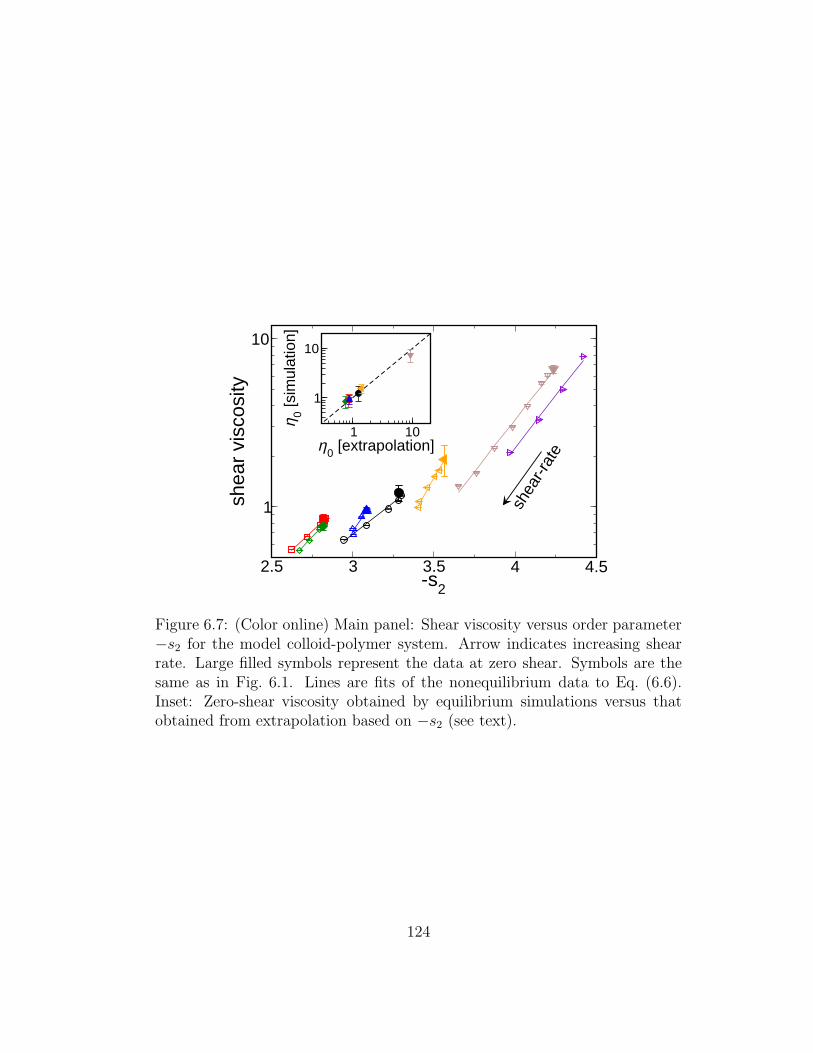
2.5 3 3.5 4 4.5-s2

1

10

shea

r vi

scos

ity

1 10η0 [extrapolation]

1

10

η 0 [sim

ulat

ion]

shea

r-rat

e

Figure 6.7: (Color online) Main panel: Shear viscosity versus order parameter−s2 for the model colloid-polymer system. Arrow indicates increasing shearrate. Large filled symbols represent the data at zero shear. Symbols are thesame as in Fig. 6.1. Lines are fits of the nonequilibrium data to Eq. (6.6).Inset: Zero-shear viscosity obtained by equilibrium simulations versus thatobtained from extrapolation based on −s2 (see text).

124

lation obeyed by the equilibrium fluid.

There are two simple potential uses for for such a relationship. Like

other constitutive equations, Eq. (6.6) provides a means for estimating the

zero-shear viscosity by extrapolation to s2 at γ = 0 (i.e., substituting the

value of s2 at zero-shear into Eq. (6.6)). Figure 6.7 demonstrates that there

is generally good agreement between the zero-shear viscosities calculated by

EMD simulations and those obtained via the aforementioned extrapolation.

Moreover, Eq. (6.6) in conjunction with theories for structure under shear

(see, e.g., [144, 145, 135, 146, 147]) provides a means to explore theoretically

the rheology of fluids.

6.3.4 Lennard-Jones Fluid

As a first test of the generality of the above structurally based constitutive

equation, we also consider the monodisperse Lennard-Jones (LJ) fluid. The

simulation details are the same as those presented above. For this model, all

quantities are reported in the standard LJ reduced form [61]. We investigate

temperatures T = 0.5, 0.75, 1.0, 1.25, packing fractions φc = πρ/6 of 0.4 and

0.45, and shear rates in the range γ = 0.005–1.0. Under these conditions,

both η and −s2 are monotonically decreasing functions of shear rate. Fig-

ure 6.8 displays η(γ) for the LJ fluid as a parametric function of −s2(γ). For

convenience, we have scaled the viscosity by ρ−2/3T−1/2, as originally suggested

by Rosenfeld [6, 7]. This scaling places the zero-shear viscosity of the dense

LJ fluid on a single curve. Again, we find that the shear-rate-dependent data

125

2 2.5 3 3.5 4 4.5-s2

2

4

8

η ρ-2

/3 T

-1/2

φc=0.4, T=0.75φc=0.4, T=1.0φc=0.4, T=1.25φc=0.45, T=0.5φc=0.45, T=0.75φc=0.45, T=1.0φc=0.45, T=1.25

2 3 4 5η0 [extrapolation]

2

3

4

5

η 0 [sim

ulat

ion]

Figure 6.8: (Color online) Main panel: Shear viscosity versus order parameter−s2 of the Lennard-Jones fluid at several values of temperature T and packingfraction φc. Large filled circles represent the data at zero shear. Solid Linesare fits of the nonequilibrium data to Eq. (6.6). Inset: Zero-shear viscosityobtained by equilibrium simulations versus those obtained from extrapolationbased on −s2 (see text).

126

is well described by Eq. (6.6). Also, as displayed in the inset to Fig. 6.8, there

is good agreement between the viscosities calculated from EMD simulations

and those obtained from the structural extrapolation. These results together

with those for the SRA fluid suggest that the structurally based constituative

equation may hold for a variety of fluids.

6.4 Conclusions

We have investigated whether two different structural aspects of a model col-

loidal fluid under shear, free volume and interparticle structural order, can be

related to the shear-rate-dependent viscosity. While the characteristic auto-

correlation time of free volumes appears to qualitatively reflect the shear vis-

cosity of the fluid, the average static free volume does not. On the other hand,

a metric for the interparticle structural order of the fluid under shear can be

quantitatively related to the shear viscosity. This latter result suggests that

the metric for structural order may be a parameter worth further study to

develop correlations between nonequilibrium structure and dynamics.

127

Chapter 7

Tuning density profiles and mobility of

inhomogeneous fluids

7.1 Introduction

Particles of confined fluids structure in an inhomogeneous manner. As a re-

sult, their relaxation processes occur at different rates than in the bulk. Al-

though density profiles of confined fluids can be predicted by classical density

functional theory (DFT), a fundamental microscopic framework for predicting

transport coefficients has yet to emerge. In fact, even an intuitive understand-

ing of how the density profile connects to dynamics is lacking.

For bulk fluids, semi-empirical structure-property relations have helped

to correlate and predict transport coefficients (see, e.g., [6, 7, 79]). Specifically,

changes in thermodynamic state variables that increase short-range structural

order of fluids are also known to decrease their mobility in a simple, quan-

tifiable way. This, as discussed in previous chapters, is true even for systems

that exhibit anomalous dynamical behavior, such as cold liquid water (where

viscosity decreases upon compression) [65, 9, 66] or concentrated colloidal

128

suspensions (where interparticle attractions increase mobility) [24, 9]. Naıve

extrapolation of this idea might lead one to suspect that inhomogeneous fluids

with highly structured (e.g., layered) density profiles would tend to be more

viscous and less diffusive than more spatially uniform fluids. Is that indeed the

case? Here, we explore this issue quantitatively. Specifically, we use molecular

simulation to investigate the relationship between the transport coefficients

of an inhomogeneous fluid and its density profile, the latter of which can be

modified in a precise way through the interactions of the fluid particles with

the confining boundaries.

A key empirical observation motivating this study is the existence of an

isothermal correlation between the self-diffusion coefficient of simple inhomoge-

neous fluids and excess entropy (relative to ideal gas), which is approximately

obeyed across a wide range of confining environments [19, 20, 21]. Specifically,

for a variety of simple model fluids, the self-diffusivity in confinement Dconfined

has approximately the same dependence on excess entropy sex as self-diffusivity

in bulk Dbulk, i.e.,

Dconfined(sex) = Dbulk(s

ex) (7.1)

Since the magnitude of the excess entropy is itself a measure of structural

order [69], the aforementioned correlation is effectively a structure-property

relationship.

Equation (7.1) provides an interesting possibility: if the excess entropy

of the confined fluid is altered, so is the mobility of the fluid. In this chapter,

we show that by changing interactions between fluid particles and the confining

129

walls, we can in turn systematically alter the excess entropy, and dynamical

properties of the fluid.

7.2 Methods

7.2.1 Model fluid

For this study, we turn to the Weeks-Chandler-Andersen (WCA) model [148],

which is known to capture the entropic packing effects that control many

properties of dense, atomistic and colloidal fluids. The WCA pair potential is

defined as

φ(r) =

4ǫ[

(

σr

)12−

(

σr

)6]

+ ǫ r < 21/6σ,

0 r > 21/6σ,

(7.2)

where r is the interparticle separation. We consider this fluid confined to a

thin film geometry between two parallel, planar boundaries placed a distance

H apart. Particles located a distance z from one boundary (0 < z < H)

interact with an external field φext(z) = φfw(z) + φfw(H − z). The single-wall

potential is given by

φfw(z) =

215

(

σz

)9−

(

σz

)3+

√10ǫ3

+ φ0(z) z < (2/5)1/6σ,

φ0(z) z > (2/5)1/6σ,

(7.3)

This represents a WCA 9-3 repulsive boundary plus an additional term φ0(z),

which can be used to tune the density profile, and excess entropy of the fluid.

130

From here forward, we simplify notation by reporting quantities implicitly

nondimensionalized by appropriate combinations of the characteristic length

scale σ and energy scale ǫ (or equivalently kBT , since we set ǫ = kBT for all

calculations). In the above, kB is the Boltzmann constant and T is tempera-

ture.

7.2.2 Tuning density profiles and excess entropy

This part of the study was performed by the collaborators Gaurav Goel and

Jefferey Errington, and thus we give only a brief description here. The inter-

ested reader is referred to [29] for further details.

The general strategy is to determine the function φ0 which alters the

excess entropy of the fluid relative to the “natural” one for the WCA fluid

confined between WCA 9-3 walls, i.e., the system with φ0(z) = 0. It was

determined via density functional theory that the excess entropy of the fluid

could be decreased by diminishing the layered structure of the density profile,

i.e., “flattening” the density profile. Likewise, the excess entropy of the fluid

could be increased by increasing the degree of layering in the fluid leading

to a “structured” density profile. Using advanced Monte Carlo simulation

techniques, the function φ0(z) that leads to both the flat and structured density

profile was determined. The form of the natural, flat, and structured profiles

are given in Fig. 7.1(a) and (b). The total potential φext which leads to these

density profiles is given in Fig. 7.1(c).

131

0 1 2 3 40

1

2

3

ρ (z

)

0 1 2 3 4z

0

10

20

30

40

50

φ ext(z

)

0 1 2 3 40

5

10

15

20

structured

flatnatural

(a) (b)

(c)

Figure 7.1: (a) Natural and flat density profiles ρ(z), and (b) natural and struc-tured density profiles for a confined WCA fluid with average density ρavg = 0.6and H = 4, as discussed in the text. (c) The associated particle-boundary in-teractions φext(z).

132

7.2.3 Simulations methods

We computed the transport coefficients of the thin films via molecular dynam-

ics simulations in the microcanonical ensemble using N = 4000 particles and

integrating the equations of motion with the velocity-Verlet algorithm [40]. A

time step of 2.5 × 10−3 was used for simulating the natural and flat profile

systems, while a shorter time step of 2×10−4 was employed for the structured

profile fluids. Periodic boundary conditions were employed in the x and y

“free” directions. We extracted values of self-diffusivity (parallel to the walls)

D by fitting the long-time (t≫ 1) behavior of the mean-squared displacement

to the Einstein relation for diffusion⟨

∆r2⟩

= 4Dt, where⟨

∆r2⟩

represents to

the mean-squared displacement in the x and y directions. Similarly, we calcu-

lated values of zero-shear viscosity η from the long-time behavior of⟨

∆A2⟩

via

its corresponding Einstein relation⟨

∆A2⟩

= 2ηT t/V . Here, ∆A =∫ t

0σxy(τ)dτ

is the time integral of the xy component of the stress tensor.

Under confinement, the excess entropy is defined as the difference be-

tween the fluid’s entropy and that of an ideal gas with the same density profile.

To obtain excess entropy data, a variety of Monte Carlo techniques were em-

ployed. Since this part of the work was performed by the collaborator Jefferey

Errington, the interested reader is referred to the original work [29] for more

details.

All simulations results are at film thickness H = 4 and average density

ρavg = H−1∫ H

0ρ(z)dz between 0.2 and 0.75.

133


In order to systematically probe the effects of flattening or enhancing the lay-

ering of the density profile, we first focus on the behavior of the confined fluid

for ρavg = 0.6 and H = 4. Let φ0,f(z) and φ0,s(z) represent the contributions

to the external potential that, under these conditions, produce the flat and

structured profiles, respectively. Starting from the natural profile, we incre-

mentally flatten the density distribution by choosing φ0(z) = λfφ0,f(z) with

progressively larger values of λf in the range 0 ≤ λf ≤ 1. Similarly, we system-

atically enhance the layering of the natural profile by setting φ0(z) = λsφ0,s(z)

with progressively larger values of λs in the range 0 ≤ λs ≤ 1.

In Fig. 7.2, we show how these specific ways of modifying the density

distribution in turn affect the entropy per particle s, the excess entropy per

particle sex, the self-diffusivity D, and the viscosity η. Observe that, by the

choice of φ0,f(z), the excess entropy is progressively decreased as λf is increased

(i.e., progressively flattening the density profile). Likewise, by the choice of

φ0,s(z), the excess entropy is progressively increases as λs is increased (i.e.,

progressively structuring the density profile).

A second important point of Fig. 7.2 is that the mobility of the confined

fluid, as measured by both η−1 and D, closely tracks the behavior of sex for the

flattening and structuring processes described above. A physical explanation

is that fluid transport parallel to the walls is dominated by interparticle colli-

sions, and hence structural correlations [6, 7, 79]. The density profile appears

to impact these transport processes mostly due to the fact that it modifies

134

1 0.5 0 0.5 1

1.5

1

2

η

0.1

0.2

D

-1

0

1

∆sex

(λ)

λ sλ f

∆sex

∆s

(a)

(b)

(c)

Figure 7.2: Effect of boundary interaction (shape of density profile) on (a)excess entropy per particle ∆sex(λ) = sex(λ) − sex(0) , (b) self-diffusivity D,and (c) viscosity η for the confined WCA fluid with ρavg = 0.6 and H = 4. Thecenterline corresponds to the fluid with the natural density profile of Fig. 1(a)and (b). From center to left, the density profile is systematically flattened:φ0(z) = λfφ0,f(z), where λf = 1 yields the flat profile shown in Fig. 1(a).From center to right, the density profile is structured: φ0(z) = λsφ0,s(z),where λs = 1 produces the structured profile shown in Fig. 1(b). Symbols aresimulation data, and curves are guide to the eye.

135

the interparticle correlations, the effect of which is conveniently isolated by

computing the excess rather than the total entropy of the fluid.

The above observation that fluids with more uniform density profiles

can actually have lower sex and slower dynamics than those with strongly

layered density profiles (and the same ρavg) appears even more general when

viewed in the context of other recent simulation data. In particular, it is now

known that the hard-sphere fluid confined between hard walls shows lower

sex [21] and slower single-particle dynamics both parallel and normal [149] to

the confining walls when such walls are separated by distances that inherently

frustrate the ability of the fluid to structure into an integer number of lay-

ers in its density profile. These model predictions of the relationship between

dynamics and density profiles can now also be readily tested in experiments,

e.g., by using confocal microsopy to investigate confined “hard-sphere” col-

loidal suspensions [150].

To document the generality of the physics discussed above, we show

in Fig. 7.3 the behaviors of sex, η, and D over a broad range of average film

densities. Perhaps most striking is the observation that, at high density, flu-

ids with structured and flat density profiles with the same ρavg can differ in

both D and η by an order of magnitude. Although the current chapter fo-

cuses on equilibrium fluid conditions, the trends evident in Fig. 7.3 suggest

that one might even be able to effectively supercool monatomic confined fluids

by isothermally modifying the external potential in a way that systematically

flattens the density profile. Finally, counterintuitive connections between or-

136

0.2 0.4 0.6ρavg

0.1

1

10

η

0.01

0.1

1

D

-5

-4

-3

-2

-1

0sex

flatnaturalstructured

(a)

(b)

(c)

Figure 7.3: (a) Excess entropy per particle sex, (b) self-diffusivity D, and (c)viscosity η, of the confined WCA fluid versus average density ρavg at H = 4.Symbols are simulation data, and curves are guide to the eye.

137

dering and dynamics have also been observed in driven systems [151, 152].

Whether one can generalize the equilibrium approach presented here to gain

insights into such non-equilibrium phenomena (e.g., the shear-induced changes

to liquid structure and viscosity [151]), however, remains an open question.

7.4 Conclusions

We have shown using molecular simulations that tuning particle-wall inter-

actions to flatten or enhance the particle layering of a model confined fluid

impacts its self-diffusivity, viscosity, and entropy. Interestingly, interactions

that eliminate particle layering significantly reduce confined fluid mobility,

whereas those that enhance layering can have the opposite effect. Excess en-

tropy provides a clear interpretation of these results

138

Chapter 8

Structural and dynamic

heterogeneities

8.1 Introduction

The emergence of heterogeneous dynamics is one of the most intriguing charac-

teristics of supercooled fluids. Dynamic processes of a fluid at high-temperatures

are homogeneous in the sense that they do not differ appreciable throughout

the fluid. In such cases, the distribution of squared displacements of parti-

cles δr2 over a time scale τ , P [log10(δr2); τ ], is unimodal. For purely random

motion, the distribution of displacements is given by [1]

P (δr, τ) = 4πδr2

(

α(τ)

π

)3/2

exp[−α(τ)δr2], (8.1)

where α(τ) = 1/4Dτ , and D is the self-diffusivity, which leads to

P [log10(δr2); τ ] = 2πln(10)δr3

(

α(τ)

π

)3/2

exp[−α(τ)δr2]. (8.2)

139

For supercooled fluids, however, the situation can be quite different [153, 154,

155, 156]. For example, P [log10(δr2); τ ] of deeply supercooled fluids, over

intermediate time intervals, may be bimodal, reflecting distinct populations of

mobile and immobile particles. This has been demonstrated by experiments

[157, 158, 84] and simulations [159, 37, 160, 161, 162, 163, 164, 165, 166, 153].

These dynamic heterogeneities have been proposed to be the origin of variety

of phenomena in supercooled liquid-state physics, such as the breakdown of

the Stokes-Einstein relationship [70, 80, 81, 82, 83] and the non-exponential

decay of relaxation processes [158, 81].

There are several open questions regarding dynamic heterogeneities.

One is the manner in which the mobile and immobile regions are spatially dis-

tributed in the fluid. Another question, which we address here, is whether dy-

namic heterogeneities reflect underlying heterogeneous structure. More specifi-

cally, is the mobility of a given particle correlated to the structural organization

around it? Here, we investigate the heterogeneous dynamics of a supercooled

hard-sphere fluid mixture. The results presented are still preliminary and

require further development. However, we are able to show evidence that het-

erogeneous dynamics are closely related to the underlying structural order of

this system.

8.2 Methods

We investigate a dense, binary hard-sphere mixture. The ratio of particle

diameters is set to σ1/σ2 = 1.3. Particle masses are proportional to their

140

volume, i.e., m1/m2 = (σ1/σ2)3. These parameters mimic recent simulation

studies [167] and experiments of colloidal suspensions [150]. We investigate

this system because it is sufficiently polydisperse to suppress crystallization,

but still the impact of particle size on the resulting properties can be unam-

biguously determined, unlike the continuously polydisperse fluids investigated

in earlier chapters.

To explore the dynamic behavior of this model system, molecular dy-

namics simulations were performed using an event-driven algorithm [61] in the

microcanonical ensemble. For all runs, N1 = N2 = 1000 particles were simu-

lated in a cubic simulation cell of volume V with periodic boundary conditions.

We investigate the model fluid at packing fractions φc = π(N1σ31 +N2σ

32)/6V

of 0.57 and 0.582, which, as we show below, lead to unimodal and bimodal

distributions of squared displacements, respectively. We have implicitly non-

dimensionalized all reported quantities in this study by appropriate com-

binations of the characteristic length scale, lc = σ2 and time scale tc =√

m2σ22/kBT , where kB is Boltzmann’s constant.


8.3.1 Quantifying dynamic heterogeneities

All reported properties are for the smaller type 2 fluid particles. However,

the results for the larger type 1 particles are qualitatively similar to those

presented here. Figure 8.1 displays the mean squared displacement (MSD)

141

10-1 10

010

1 102

103

104 10

5

t

10-2

10-1

100

101

<δr2 >

φ c=0

.57

φ c=0

.582

Figure 8.1: Mean-square displacement 〈δr2〉 of the small type 2 particles versustime at packing fraction φc = 0.57 (black) and 0.582 (red). Dashed lines arefits of 〈δr2〉 = 6Dt to the long time behavior resulting in D = 1.2 × 10−3 and1.5 × 10−4 at φc = 0.57 and 0.582, respectively.

142

〈δr2〉 at packing fractions φc = 0.57 and 0.58 of the small type 2 particles

versus time. Note that in both cases that the MSD displays a plateau at

intermediate times. This behavior is characteristic of “cage” dynamics in the

system [168], where particles are confined by well defined cages formed by

neighboring particles. At very short times, particles move ballistically within

their particle cage. At intermediate times, motion is significantly impeded by

the cage, which leads to the plateau in 〈δr2〉. The displacement at the plateau

decreases as φc increases, indicating a smaller cage size. Also, the plateau

persists for longer times as φc increases, indicating a longer lifetime for cages.

At longer times, particle motion becomes diffusive (i.e., 〈δr2〉 = 6Dt, fit shown

in Fig. 8.1).

How do the microscopic (single-particle) mobilities behave? The distri-

bution of the logarithm of squared displacements δr2 over a time interval τ ,

P [log10(δr2); τ ], provides a simple way to quantify microscopic rearrangements

[169]. Figure 8.2 displays P [log10(δr2); τ ] at several values of τ for the small

type 2 particles at φc = 0.57. Note that all time intervals investigated are larger

than that associated with ballistic motion. At all values of τ , P [log10(δr2); τ ] is

unimodal. However, we observe that the P [log10(δr2); τ ] over the smaller time

windows display slight, but distinguishable, enhancements of probabilities of

larger displacements, particularly at τ = 50. This appears to be a precursor

to the behavior at φc = 0.582 which we discuss in detail below.

Figure 8.3 displays the behavior of P [log10(δr2); τ ] at several values of τ

for the small type 2 particles at φc = 0.582. We observe that, for intermediate

143

-3 -2 -1 0 1 2

log10(δr2)

0

0.2

0.4

0.6

0.8

1

P[lo

g 10(δ

r2 ) ; τ

]

25

50

100250

500

1000

Figure 8.2: Distribution of the logarithm of squared displacementsP [log10(δr

2); τ ] at several values of τ at packing fraction φc = 0.57 for thesmall type 2 particles. The numbers in the figure correspond to the value of τfor the curve of the same color.

144

-2 0 2

log10(δr2)

0

0.2

0.4

0.6

0.8

1

P[lo

g 10(δ

r2 ) ; τ

]

500

1000

2000

4000

8000

16000

16

Figure 8.3: Distribution of the logarithm of squared displacementsP [log10(δr

2); τ ] at several values of τ at packing fraction φc = 0.582 for thesmall type 2 particles. The numbers in the figure correspond to the value of τfor the curve of the same color. Vertical line is at δr2 = 0.56, the approximatedividing line between mobile and immobile particles (see text).

145

time intervals (500 ≤ τ ≤ 4000), P [log10(δr2); τ ] is bimodal. That is, there

are distinct populations of mobile and immobile particles with a boundary

between the two populations at δr2 ≈ 0.56 (vertical dashed line in Fig. 8.1).

Particles with δr2 < 0.56 are termed immobile, while those δr2 > 0.56 are

termed mobile. This behavior is in stark contrast to that of the fluid at

lower packing fractions. The basic physics behind the behavior depicted in

Fig. 8.3 has been well documented [170] and can be explained as follows. Over

short times, particles are confined to their cages and are hence immobile.

Eventually, a rare, collective rearrangement allows a particle to move over a

larger distance (approximately one particle diameter), i.e., to “hop” to a new

position, making it mobile. Over an increasingly long time interval, more of

these hopping events occur, and hence the number of mobile particles increase.

Over sufficiently long time intervals, almost all particles are able to move and

the P [log10(δr2); τ ] again becomes unimodal.

8.3.2 Structure of mobile and immobile particles.

The central question we wish to address is whether there is a connection be-

tween the mobility of a particle and the structure around it over a given time

interval. Our approach to this problem is motivated by the connection be-

tween transport properties and the two-body excess entropy s2. As has been

discussed at length in this thesis, the self-diffusivity is well described by the

146

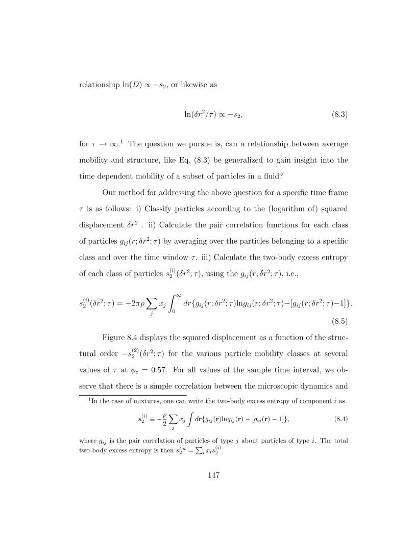
relationship ln(D) ∝ −s2, or likewise as

ln(δr2/τ) ∝ −s2, (8.3)

for τ → ∞.1 The question we pursue is, can a relationship between average

mobility and structure, like Eq. (8.3) be generalized to gain insight into the

time dependent mobility of a subset of particles in a fluid?

Our method for addressing the above question for a specific time frame

τ is as follows: i) Classify particles according to the (logarithm of) squared

displacement δr2 . ii) Calculate the pair correlation functions for each class

of particles gij(r; δr2; τ) by averaging over the particles belonging to a specific

class and over the time window τ . iii) Calculate the two-body excess entropy

of each class of particles s(i)2 (δr2; τ), using the gij(r; δr

2; τ), i.e.,

s(i)2 (δr2; τ) = −2πρ

∑

j

xj

∫ ∞

0

dr{gij(r; δr2; τ)lngij(r; δr

2; τ)−[gij(r; δr2; τ)−1]}.

(8.5)

Figure 8.4 displays the squared displacement as a function of the struc-

tural order −s(2)2 (δr2; τ) for the various particle mobility classes at several

values of τ at φc = 0.57. For all values of the sample time interval, we ob-

serve that there is a simple correlation between the microscopic dynamics and

1In the case of mixtures, one can write the two-body excess entropy of component i as

s(i)2 ≡ −

ρ

2

∑

j

xj

∫

dr{gij(r)lngij(r) − [gij(r) − 1]}, (8.4)

where gij is the pair correlation of particles of type j about particles of type i. The total

two-body excess entropy is then stot2 =

∑

i xis(i)2 .

147

5 5.2 5.4 5.6

-s2(2)

[δr2;τ]

-2

-1

0

1

2

log 10

[δr2 (τ

)]

τ=25

50100

250500 1000

Figure 8.4: Logarithm of squared displacements log10[δr2(τ)] versus structural

order −s(2)2 (δr2; τ) for the various particle mobility classes at several values of

time interval τ at φc = 0.57. The numbers in the figure correspond to the valueof τ for the curve of the same color. The size of the symbols are proportionalto the fraction of particles belonging to each mobility class.

148

structural order. Explicitly, increasing the degree of structural order [increas-

ing −s(2)2 (δr2; τ)] is seen to correlate with a reduction in mobility over that

time interval. The slope of the correlation between mobility and −s(2)2 (δr2; τ)

becomes more negative at larger times. This implies that the fluctuations

in structural order [i.e., the range of values of −s(2)2 (δr2; τ)] become less pro-

nounced than the fluctuations in mobility (the range of values of log10[δr2(τ)])

over increasing time intervals. We are unaware of other predictions for fluctu-

ations in structure of this kind even for very simple model fluids.

5.5 6 6.5

-s2(2)

[δr2;τ]

-2

-1

0

1

log 10

[δr2 (τ

)]

τ=500

100020004000

8000

16000

Figure 8.5: Logarithm of squared displacements log10[δr2(τ)] versus structural

order −s(2)2 (δr2; τ) for the various particle mobility classes at several values

of time interval τ at φc = 0.582. The numbers in the figure correspond tothe value of τ for the curve of the same color. The size of the symbols areproportional to the fraction of particles belonging to each mobility class. Hor-izontal dashed line at δr2 = 0.56, the boundary between mobile and immobileparticles (see Fig. 8.3 and text).

149

Figure 8.5 displays the squared displacement as a function of the struc-

tural order for the various particle mobility classes at several values of τ at

φc = 0.582. There are several important features of this figure. Foremost,

similar to the system at lower packing fraction, significant mobility appears to

require a critical amount of local disorder. Consider, for example, the τ = 500

case. For a particle to be mobile (i.e., to the left of the dashed line in Fig. 8.3

or above the dashed line in Fig. 8.5, also at δr2 = 0.56), it on average has

−s(2)2 (δr2; τ) . 5.5. We also observe that, unlike in the lower packing frac-

tion case, there is a non-monotonic shape (an oscillation) in the correlation

at lower values of −s(2)2 (δr2; τ). The shape of the curve suggests, perhaps, a

sequence of events for the mobile particles. As discussed above, it is relatively

well established that it is the “hopping” particles which are mobile. Before

a particle can make a hop, it must first attain a certain degree of disorder.

After a particle makes a hop however, it regains a certain degree of order,

with its neighbors reforming a cage structure around it. This leads to the

oscillation observed in the correlation between mobility and structural order,

and also differentiates the dynamically heterogeneous case (φc = 0.582) from

the dynamically homogeneous case (φc = 0.57). A schematic of our hypothesis

regarding this sequence is displayed in Fig. 8.6. Over increasingly long time

intervals, the oscillation in the correlation as well as the critical amount of dis-

order required to be mobile are diminished. This indicates that, as expected,

structural correlations associated with the hopping process become smeared

out over long times.

150

R e g a i n o r d e r a f t e rd i s p l a c e m e n t

C r i t i c a l d i s o r d e r t om a k e d i s p l a c e m e n tFigure 8.6: Schematic of structure of particles just before and just after a hop.

151

An obvious question at this stage is whether the above correlation be-

tween single-particle dynamics and structural order is due simply to changes

in local density. To determine if this is the case, we calculate the number of

nearest neighbors around the type 2 particles for the various mobility classes

and time intervals, n(2)tot(δr

2; τ), defined as

n(2)tot(δr

2; τ) ≡∑

j

4πxjρ

∫ rmin

0

r2g2j(r; δr2; τ)dr (8.6)

where ρ is the total number density, xj is the mole fraction of component j

and rmin is the location of the first minimum in g2j(r; δr2; τ).

Figure 8.6(a) and (b) display n(2)tot(δr

2; τ) for φc = 0.57 and 0.582, respec-

tively. At both packing fractions, there is no systematic correlation between

mobility and number of nearest neighbors. That is, the number of nearest

neighbors is almost constant for the various mobility classes. Therefore, local

density (at least by this measure) does not account for the correlation between

structural order and single particle mobilities noted above.

8.4 Conclusions

Using molecular simulations, we have shown that the mobility of particles is

correlated to the structure of the particles surrounding them. Specifically,

we have demonstrated that particles on average require a critical amount of

disorder in order to be mobile on intermediate time scales. In future work,

we will address the specific features of the structural order around mobile and

152

11

11.5

12

n tot

(2) [δ

r2 ;τ]

-3 -2 -1 0 1 2

log10[δr2(τ)]

11

11.5

(a) φc=0.57

(b) φc=0.582

Figure 8.7: Number of nearest neighbors around the type 2 particles for variousmobility classes and time windows, n

(2)tot(δr

2; τ), at (a) φc = 0.57 and (b) φc =0.58. The symbols in (a) and (b) are the same as those in Figs. 8.4 and8.5, respectively. The size of the symbols are proportional to the fraction ofparticles belonging to each mobility class.

153

immobile particles (much like the analysis of Chapter 5). We also hope to tie

the dynamic aspects of this investigation to the static structural characteristics

of the fluid.

154

Bibliography

[1] J. P. Hansen and I. R. McDonald. Theory of Simple Liquids. Academic,

London, 3rd edition, 2006.

[2] P. G. Debenedetti. Metastable Liquids. Concepts and Principles. Prince-

ton University Press, Princeton New Jersey, 1996.

[3] A. K. Doolittle. Studies in newtonian flow. II. The dependence of the

viscosity of liquids on free-space. J. Appl. Phys., 22:1471, 1951.

[4] H. Liu, C. M. Silva, and E. A. Macedo. Genaralised free-volume theory

for transport properties and new trends about the relationship between

free volume and equations of state. Fluid Phase Equilib., 202:89, 2002.

[5] J. Mittal, J. R. Errington, and T. M. Truskett. Relationship between

thermodynamics and dynamics of supercooled liquids. J. Chem. Phys.,

125:076102, 2006.

[6] Y. Rosenfeld. Relation between the transport coefficients and the inter-

nal entropy of simple systems. Phys. Rev. A, 15:2545–2549, 1977.

[7] Y. Rosenfeld. A quasi-universal scaling law for atomic transport in sim-

ple fluids. J. Phys.: Condens. Matter, 11:5415, 1999.

[8] R. E. Nettleton and M. S. Green. Expression in terms of molecular

distribution functions for the entropy density in an infinite system. J.

Chem. Phys., 29:1365–1370, 1958.

[9] J. Mittal, J. R. Errington, and T. M. Truskett. Quantitative link between

single-particle dynamics and static structure of supercooled liquids. J.

Phys. Chem. B, 110:18147–18150, 2006.

155

[10] J. D. Weeks, D. Chandler, and H. C. Andersen. Role of repulsive forces

in determining the equilibrium structure of simple liquids. J. Chem.

Phys., 54:5237–5247, 1971.

[11] S. Sastry, T. M. Truskett, P. G. Debenedetti, and S. Torquato. Free

volume in the hard sphere liquid. Mol. Phys., 95:289, 1998.

[12] W. B. Russel, D. A. Saville, and W. R. Schowalter. Colloidal Dispersions.

Cambridge University Press, New York, 1989.

[13] F. Sciortino. One liquid, two glasses. Nat. Mater., 1:145, 2002.

[14] S. Asakura and F. Oosawa. On interaction between two bodies immersed

in a solution of macromolecules. J. Chem. Phys., 22:1255, 1954.

[15] T. Eckert and E. Bartsch. Re-entrant glass transition in a colloid-

polymer mixture with depletion attractions. Phys. Rev. Lett., 89:125701,

2002.

[16] K. N. Pham, A. M. Puertas, J. Bergenholtz, S. U. Egelhaaf, A. Moussaıd,

P. N. Pusey, A. B. Schofield, M. E. Cates, M. Fuchs, and W. C. K. Poon.

Multiple glassy states in a simple model system. Science, 296:104, 2002.

[17] J. Bergenholtz and M. Fuchs. Nonergodicity transitions in colloidal sus-

pensions with attractive interactions. Phys. Rev. E, 59:5706–5715, 1999.

[18] L. Fabbian, W. Gotze, F. Sciortino, P. Tartaglia, and F. Thiery. Ideal

glass-glass transitions and logarithmic decay of correlations in a simple

system. Phys. Rev. E, 59:R1347, 1999.

[19] J. Mittal, J. R. Errington, and T. M. Truskett. Thermodynamics predicts

how confinement modifies the dynamics of the equilibrium hard-sphere

fluid. Phys. Rev. Lett., 96:177804, 2006.

156

[20] J. Mittal, J. Errington, and T. Truskett. Relationships between self-

diffusivity, packing fraction, and excess entropy in simple bulk and con-

fined fluids. J. Phys. Chem. B, 111:10054–10063, 2007.

[21] J. Mittal, J. R. Errington, and T. M. Truskett. Does confining the hard-

sphere fluid between hard walls change its average properties? J. Chem.

Phys., 126:244708, 2007.

[22] W. P. Krekelberg, V. Ganesan, and T. M. Truskett. Free volumes and

the anomalous self-diffusivity of attractive colloids. J. Phys. Chem. B,

110:5166, 2006.

[23] W. P. Krekelberg, V. Ganesan, and T. M. Truskett. Model for the free-

volume distributions of equilibrium fluids. J. Chem. Phys., 124:214502,

2006.

[24] W. P. Krekelberg, J. Mittal, V. Ganesan, and T. M. Truskett. How

short-range attractions impact the structural order, self-diffusivity, and

viscosity of a fluid. J. Chem. Phys., 127:044502, 2007.

[25] W. P. Krekelberg, J. Mittal, V. Ganesan, and T. M. Truskett. Structural

anomalies of fluids: Origins in second and higher coordination shells.

Phys. Rev. E, 77:041201, 2008.

[26] Z. Yan, S. V. Buldyrev, P. Kumar, N. Giovambattista, P. G. Debenedetti,

and H. E. Stanley. Structure of the first- and second-neighbor shells of

simulated water: Quantitative relation to translational and orientational

order. Phys. Rev. E, 76:051201, 2007.

[27] W. P. Krekelberg, V. Ganesan, and T. M. Truskett. Shear-rate-

dependent structural order and viscosity of a fluid with short-range at-

tractions. Phys. Rev. E, 2008. in press.

157

[28] W. P. Krekelberg, T. M. Truskett, and V. Ganesan. Relationship be-

tween viscosity and some structural aspects of a colloidal suspension.

Chem. Eng. Commun., 2008. in press.

[29] G. Goel, W. P. Krekelberg, J. R. Errington, and T. M. Truskett. Tuning

density profiles and mobility of inhomogeneous fluids. Phys. Rev. Lett.,

100:106001, 2008.

[30] P. Germain and S. Amokrane. Validity of the perturbation theory for

hard particle systems with very-short-range attraction. Phys. Rev. E,

65:031109, 2002.

[31] P. J. Camp. Phase diagrams of hard spheres with algebraic attractive

interactions. Phys. Rev. E, 67:011503, 2003.

[32] K. Dawson, G. Foffi, M. Fuchs, W. Gotze, F. Sciortino, M. Sperl,

P. Tartaglia, T. Voigtmann, and E. Zaccarelli. Higher-order glass-

transition singularities in colloidal systems with attractive interactions.

Phys. Rev. E, 63:011401–1–011401–17, 2000.

[33] E. Zaccarelli, G. Foffi, K. A. Dawson, S. V. Buldyrev, F. Sciortino, and

P. Tartaglia. Confirmation of anomalous dynamical arrest in attractive

colloids: A molecular dynamics study. Phys. Rev. E, 66:041402, 2002.

[34] A. M. Puertas, M. Fuchs, and M. E. Cates. Comparative simulation

study of colloidal gels and glasses. Phys. Rev. Lett., 88:098301, 2002.

[35] A. M. Puertas, M. Fuchs, and M. E. Cates. Simulation study of non-

ergodicity transitions: Gelation in colloidal systems with short-range

attractions. Phys. Rev. E, 67:031406, 2003.

[36] A. M. Puertas, M. Fuchs, and M. E. Cates. Dynamical heterogeneities

close to a colloidal gel. J. Chem. Phys., 121:2813, 2004.

158

[37] D. R. Reichman, E. Rabani, and P. L. Geissler. Comparison of dynam-

ical heterogeneity in hard-sphere and attractive glass formers. J. Phys.

Chem. B, 109:14654, 2005.

[38] A. M. Puertas, M. Fuchs, and M. E. Cates. Mode coupling and dynamical

heterogeneity in colloidal gelation: A simulation study. J. Phys. Chem.

B, 109:6666, 2005.

[39] S. Asakura and F. Oosawa. Interaction between particles suspended in

solutions of macromolecules. J. Polym. Sci. Polym. Symp., 33:183–192,

1958.

[40] M. P. Allen and D. J. Tildesley. Computer Simulations of Liquids. Oxford

University Press, New York, 1987.

[41] W. G. Hoover, W. T. Ashurst, and R. Grover. Exact dynamical basis

for a fluctuating cell model. J. Chem. Phys., 57:1259, 1972.

[42] S. Sastry, D. S. Corti, P. G. Debenedetti, and F. H. Stillinger. Statistical

geometry of particle packings. I. Algorithm for exact determination of

connectivity, volume, and surface areas of void space in monodisperse

and polydisperse sphere packings. Phys. Rev. E, 56:5524, 1997.

[43] F. W. Starr, S. Sastry, J. F. Douglas, and S. C. Glotzer. What do we

learn from the local geometry of glass-forming liquids. Phys. Rev. Lett.,

89:125501, 2002.

[44] J. P. Hansen and I. R. McDonald. Theory of Simple Liquids. Academic,

London, 2nd ed edition, 1986.

[45] W. Gotze. Recent tests of the mode-coupling theory for glassy dynamics.

J. Phys.: Condens. Matter, 11:A1, 1999.

[46] D. R. Reichman and P. Charbonneau. Mode-coupling theory. J. Stat.

Mech., page P05013, 2005.

159

[47] R. J. Speedy. Cavities and free-volume in hard-disk and hard-sphere

systems. J. Chem. Soc., Faraday Trans. 2, 77:329, 1981.

[48] R. J. Speedy and H. Reiss. A computer-simulation study of cavities in

the hard disk fluid and crystal. Mol. Phys., 72:1015, 1991.

[49] D. S. Corti and R. K. Bowles. Statistical geometry of hard sphere sys-

tems: exact relations for additive and non-additive mixtures. Mol. Phys.,

96:1623, 1999.

[50] A. Rahman. Liquid structure and self-diffusion. J. Chem. Phys., 45:

2585, 1966.

[51] M. H. Cohen and D. Turnbull. Molecular transport in liquids and glasses.

J. Chem. Phys., 31:1164, 1959.

[52] M. H. Cohen and G. S. Grest. Liquid-glass transition, a free-volume

approach. Phys. Rev. B, 20:1077, 1979.

[53] J. C. Conrad, F. W. Starr, and D. A. Weitz. Weak correlations between

local density and dynamics near the glass transition. J. Phys. Chem. B,

109:21235, 2005.

[54] R. P. A. Dullens, D. G. A. L. Aarts, and W. K. Kegel. Direct measure-

ment of the free energy by optical microscopy. Proc. Natl. Acad. Sci.

USA, 103:529, 2006.

[55] P. G. Debenedetti and T. M. Truskett. The statistical geometry of voids

in liquids. Fluid Phase Equilib., 158:549, 1999.

[56] S. Torquato, T. M. Truskett, and P. G. Debenedetti. Is random close

packing of spheres well defined? Phys. Rev. Lett., 84:2064, 2000.

[57] F. Gursey. Classical statistical mechanics of a rectilinear assembly. Proc.

Cambridge Philos. Soc, 46:182, 1950.

160

[58] L. Tonks. The complete equation of state of one, two and three-

dimensional gases of hard elastic spheres. Phys. Rev., 50:955, 1936.

[59] G. Ruocco and M. Sampoli. Geometrical aspects of self-diffusion in liquid

water. J. Mol. Struct., 250:171, 1991.

[60] G. Ruocco and M. Sampoli. Self-diffusion in liquid water-a geometrical

approach. Chem. Phys. Lett., 188:332, 1992.

[61] D. C. Rapaport. The Art of Molecular Dynamic Simulation. Cambridge

University Press, Cambridge, 2nd edition, 2004.

[62] N. F. Carnahan and K. E. Starling. Equation of state for nonattracting

rigid spheres. J. Chem. Phys., 51:635, 1969.

[63] J. R. Errington and P. G. Debenedetti. Relationship between structural

order and the anomalies of liquid water. Nature, 409:318–321, 2001.

[64] S. Sastry. Water structure: Order and oddities. Nature, 409:300–301,

2001.

[65] J. R. Errington, T. M. Truskett, and J. Mittal. Excess-entropy-based

anomalies for water like fluid. J. Chem. Phys., 125:244502, 2006.

[66] R. Sharma, S. N. Chakraborty, and C. Chakravarty. Entropy, diffusivity,

and structural order in liquids with waterlike anomalies. J. Chem. Phys.,

125:204501, 2006.

[67] G. Foffi, K. A. Dawson, S. V. Buldyrev, F. Sciortino, E. Zaccarelli, and

P. Tartaglia. Evidence for an unusual dynamical-arrest scenario in short-

ranged colloidal system. Phys. Rev. E, 65:050802(R), 2002.

[68] B. J. Alder, D. M. Gass, and T. E. Wainwright. Studies in molecular

dynamics. viii. the transport coefficients for a hard-sphere fluid. J. Chem.

Phys., 53:3813, 1970.

161

[69] T. M. Truskett, S. Torquato, and P. G. Debenedetti. Towards a quan-

tification of disorder in materials: Distinguishing equilibrium and glassy

sphere packings. Phys. Rev. E, 62:993, 2000.

[70] S. K. Kumar, G. Szamel, and J. F. Douglas. Nature of the breakdown in

the stokes-einstein relationship in a hard sphere fluid. J. Chem. Phys.,

124:214501, 2006.

[71] E. Rossler. Indications for a change of diffusion mechanism in super-

cooled liquids. Phys. Rev. Lett., 65:1595–1598, 1990.

[72] M. T. Cicerone, F. R. Blackburn, and M. D. Ediger. How do molecules

move near tg? molecular rotation of six probes in o-terphenyl across 14

decades in time. J. Chem. Phys., 102:471–479, 1995.

[73] M. T. Cicerone and M. D. Ediger. Photobleaching technique for measur-

ing ultraslow reorientation near and below the glass transition: Tetracene

in o-terphenyl. J. Phys. Chem., 97:10489, 1993.

[74] F. Fujara, B. Geil, H. Sillescu, and G. Fleischer. Translational and ro-

tational diffusion in supercooled orthoterphenyl close to the glass tran-

sition. Z. Phys. B., 88:195, 1992.

[75] Z. Yan, S. V. Buldyrev, N. Giovambattista, P. G. Debenedetti, and H. E.

Stanley. Family of tunable spherically symmetric potentials that span

the range from hard spheres to waterlike behavior. Phys. Rev. E, 73:

051204, 2006.

[76] A. B. de Oliveira, P. A. Netz, T. Colla, and M. C. Barbosa. Structural

anomalies for a three dimensional isotropic core-softened potential. J.

Chem. Phys., 125:124503, 2006.

[77] A. B. de Oliveira, P. A. Netz, T. Colla, and M. C. Barbosa. Ther-

modynamic and dynamic anomalies for a three-dimensional isotropic

core-softened potential. J. Chem. Phys., 124:084505, 2006.

162

[78] M. S. Shell, P. G. Debenedetti, and A. Z. Panagiotopoulos. Molecular

structural order and anomalies in liquid silica. Phys. Rev. E, 66:011202,

2002.

[79] M. Dzugutov. A univeral scaling law for atomic diffusion in condesed

matter. Nature, 381:137–139, 1996.

[80] R. Yamamoto and A. Onuki. Heterogeneous diffusion in highly super-

cooled liquids. Phys. Rev. Lett., 81:4915–4918, 1998.

[81] M. D. Ediger. Spatially heterogeneous dynamics in supercooled liquids.

Annu. Rev. Phys. Chem., 51:99, 2000.

[82] F. H. Stillinger and J. A. Hodgdon. Translation-rotation paradox for

diffusion in fragile glass-forming liquids. Phys. Rev. E, 50:2064–2068,

1994.

[83] G. Tarjus and D. Kivelson. Breakdown of the stokes–einstein relation in

supercooled liquids. J. Chem. Phys., 103:3071–3073, 1995.

[84] E. R. Weeks, J. C. Crocker, A. C. Levitt, A. Schofield, and D. A. Weitz.

Three-dimensional direct imaging of structural relaxation near the col-

loidal glass transition. Science, 287:627–631, 2000.

[85] H. Lowen. Fun with hard spheres. In K. R. Mecke and D. Stoyan,

editors, Statistical Physics and Spatial Statistics, volume 554 of Lecture

Notes in Physics, page 295. Springer, Berlin, 2000.

[86] S. Chapman and T. G. Cowling. The Mathematical Theory of Non-

uniform Gases. Cambridge University Press, 3rd edition, 1970.

[87] G. Nemethy and H. A. Scheraga. Structure of water and hydropho-

bic bonding in proteins. II. Model for the thermodynamic properties of

aqueous solutions of hydrocarbons. J. Chem. Phys., 36:3401–3417, 1962.

163

[88] L. R. Pratt. Theory of hydrophobic effects. Annu. Rev. Phys. Chem.,

36:433–449, 1985.

[89] D. Beglov and B. Roux. Finite representation of an infinite bulk system:

Solvent boundary potential for computer simulations. J. Chem. Phys.,

100:9050–9063, 1994.

[90] N. Matubayasi, L. H. Reed, and R. M. Levy. Thermodynamics of the hy-

dration shell. 1. Excess energy of a hydrophobic solute. J. Phys. Chem.,

98:10640, 1994.

[91] K. A. T. Silverstein, A. D. J. Haymet, and K. A. Dill. Molecular model

of hydrophobic solvation. J. Chem. Phys., 111:8000–8009, 1999.

[92] D. M. Lockwood and P. J. Rossky. Evaluation of functional group con-

tributions to excess volumetric properties of solvated molecules. J. Phys.

Chem. B, 103:1982–1990, 1999.

[93] D. M. Lockwood, P. J. Rossky, and R. M. Levy. Functional group contri-

butions to partial molar compressibilities of alcohols in water. J. Phys.

Chem. B, 104:4210–4217, 2000.

[94] G. Hummer, S. Garde, A. E. Garcia, and L. R. Pratt. New perspectives

on hydrophobic effects. Chem. Phys., 258:349–370, 2000.

[95] M. E. Paulaitis, L. R. Pratt, and G. D. Rose. Hydration theory for

molecular biophysics. Adv. Protein Chem., 62:283–310, 2002.

[96] D. Asthagiri, L. R. Pratt, M. E. Paulaitis, and S. B. Rempe. Hydration

structure and free energy of biomolecularly specific aqueous dications,

including Zn2+ and first transition row metals. J. Am. Chem. Soc., 126:

1285–1289, 2004.

[97] K. A. Dill, T. M. Truskett, V. Vlachy, and B. Hribar-Lee. Modeling

water, the hydrophobic effect, and ion solvation. Annu. Rev. Biophys.

Biomol. Struct., 34:173–199, 2005.

164

[98] T. M. Truskett, S. Torquato, S. Sastry, P. G. Debenedetti, and F. H.

Stillinger. Structural precursor to freezing in the hard-disk and hard-

sphere systems. Phys. Rev. E, 58:3083–3088, 1998.

[99] J. L. Finney. Random packings and the structure of simple liquids. I.

The geometry of random close packing. Proc. R. Soc. London, Ser. A,

319:479–493, 1970.

[100] C. H. Bennett. Serially deposited amorphous aggregates of hard spheres.

J. Appl. Phys., 43:2727–2734, 1972.

[101] A. Rahman, M. J. Mandell, and J. P. McTague. Molecular dynamics

study of an amorphous lennard-jones system at low temperature. J.

Chem. Phys., 64:1564–1568, 1976.

[102] F. H. Stillinger and T. A. Weber. Packing structures and transitions in

liquids and solids. Science, 225:983–989, 1984.

[103] Y. J. Hiwatari, T. Saito, and A. J. Ueda. Structural characterization of

soft-core and hard-core glasses by delaunay tessellation. J. Chem. Phys.,

81:6044, 1984.

[104] A. S. Clarke and J. D. Wiley. Numerical simulation of the dense random

packing of a binary mixture of hard spheres: Amorphous metals. Phys.

Rev. B, 35:7350–7356, 1987.

[105] K. Tsumuraya and M. S. Watanabe. Local structure and stability in a

model glass. J. Chem. Phys., 92:4983–4992, 1990.

[106] I. Snook, W. van Megen, and P. Pusey. Structure of colloidal glasses

calculated by the molecular-dynamics method and measured by light

scattering. Phys. Rev. A, 43:6900–6907, 1991.

[107] A. Donev, S. Torquato, and F. H. Stillinger. Pair correlation function

characteristics of nearly jammed disordered and ordered hard-sphere

packings. Phys. Rev. E, 71:011105, 2005.

165

[108] B. O’Malley and I. Snook. Structure of hard-sphere fluid and precursor

structures to crystallization. J. Chem. Phys., 123:054511, 2005.

[109] M. Dzugutov, S. I. Simdyankin, and F. H. M. Zetterling. Decoupling

of diffusion from structural relaxation and spatial heterogeneity in a

supercooled simple liquid. Phys. Rev. Lett., 89:195701, 2002.

[110] T. S. Jain and J. J. de Pablo. Role of local structure on motions on the

potential energy landscape for a model supercooled polymer. J. Chem.

Phys., 122:174515, 2005.

[111] H. Shintani and H. Tanaka. Frustration on the way to crystallization in

glass. Nat. Phys., 2:200–206, 2006.

[112] T. Kawasaki, T. Araki, and H. Tanaka. Correlation between dynamic

heterogeneity and medium-range order in two-dimensional glass-forming

liquids. Phys. Rev. Lett., 99:215701, 2007.

[113] T. M. Truskett and K. A. Dill. A simple statistical mechanical model of

water. J. Phys. Chem. B, 106:11829–11842, 2002.

[114] Z. Yan, S. V. Buldyrev, N. Giovambattista, and H. E. Stanley. Structural

order for one-scale and two-scale potentials. Phys. Rev. Lett., 95:130604,

2005.

[115] A. B. de Oliveira, M. C. Barbosa, and P. A. Netz. Interplay between

structure and density anomaly for an isotropic core-softened ramp-like

potential. Physica A, 386:744–747, 2007.

[116] M. Agarwal, R. Sharma, and C. Chakravarty. Ionic melts with waterlike

anomalies: Thermodynamic properties of liquid BeF2. J. Chem. Phys.,

127:164502, 2007.

[117] M. Agarwal and C. Chakravarty. Waterlike structural and excess entropy

anomalies in liquid beryllium fluoride. J. Phys. Chem. B, 111:13294–

13300, 2007.

166

[118] A. B. de Oliveira, G. Franzese, P. A. Netz, and M. C. Barbosa. Waterlike

hierarchy of anomalies in a continuous spherical shouldered potential. J.

Chem. Phys., 128:064901, 2008.

[119] M. W. Mahoney and W. L. Jorgensen. A five-site model for liquid water

and the reproduction of the density anomaly by rigid, nonpolarizable

potential functions. J. Chem. Phys., 112:8910–8922, 2000.

[120] H. J. C. Berendsen, J. R. Grigera, and T. P. Straatsma. The missing

term in effective pair potentials. J. Phys. Chem., 91:6269 – 6271, 1987.

[121] P. Kumar, S. V. Buldyrev, F. Sciortino, E. Zaccarelli, and H. E. Stan-

ley. Static and dynamic anomalies in a repulsive spherical ramp liquid:

Theory and simulation. Phys. Rev. E, 72:021501, 2005.

[122] R. Esposito, F. Saija, A. M. Saitta, and P. V. Giaquinta. Entropy-based

measure of structural order in water. Phys. Rev. E, 73:040502(R), 2006.

[123] P. A. Netz, S. V. Buldyrev, M. C. Barbosa, and H. E. Stanley. Ther-

modynamic and dynamic anomalies for dumbbell molecules interacting

with a repulsive ramplike potential. Phys. Rev. E, 73:061504, 2006.

[124] L. Xu, S. V. Buldyrev, C. A. Angell, and H. E. Stanley. Thermodynamics

and dynamics of the two-scale spherically symmetric jagla ramp model

of anomalous liquids. Phys. Rev. E, 74:031108, 2006.

[125] M. M. Szortyka and M. C. Barbosa. Diffusion anomaly in an associating

lattice gas model. Physica A, 380:27–35, 2007.

[126] L. S. Ornstein and F. Zernike. integral equation. Proc. R. Acad. Sci.

Amsterdam, 17:793, 1914.

[127] S. Labık, A. Malijevsky, and P. Vonka. A rapidly convergent method of

solving the oz equation. Mol. Phys., 56:709–715, 1985.

167

[128] J. K. Percus and G. J. Yevick. Analysis of classical statistical mechanics

by means of collective coordinates. Phys. Rev., 110:1–13, 1958.

[129] J. M. J. van Leeuwen, J. Groeneveld, and J. de Boer. New method for

the calculation of the pair correlation function. I. Physica, 25:792–808,

1959.

[130] A. A. Louis, P. G. Bolhuis, and J. P. Hansen. Mean-field fluid behavior

of the gaussian core model. Phys. Rev. E, 62:7961–7972, 2000.

[131] A. Baranyai and D. J. Evans. Direct entropy calculation from computer

simulation of liquids. Phys. Rev. A, 40:3817–3822, 1989.

[132] J. Mittal, W. P. Krekelberg, J. R. Errington, and T. M. Truskett. Com-

puting free volume, structural order, and entropy of liquids and glasses.

In K. B. Lipkowitz and T. R. Cundari, editors, Reviews in Computa-

tional Chemistry, volume 25, pages 125–158. Wiley-VCH, New Jersey,

2007.

[133] F. Sciortino, A. Geiger, and H. E. Stanley. Effect of defects on molecular

mobility in liquid water. Nature, 354:218–221, 1991.

[134] Z. Yan, S. V. Buldyrev, P. Kumar, N. Giovambattista, and H. E. Stan-

ley. Correspondence between the phase diagrams of tip5p water and

a spherically symmetric repulsive ramp potential. arXiv:0712.2048v1,

2007.

[135] J. F. Brady. The rheological behavior of concentrated colloidal disper-

sions. J. Chem. Phys., 99:567–581, 1993.

[136] R. A. Lionberger and W. B. Russel. Microscopic theories of the rheology

of stable colloidal dispersions. In I. Prigogine and S. A. Rice, editors,

Advances in Chemical Physics, volume 111, pages 399–474. Wiley, New

York, 2000.

168

[137] C. McCabe, C. W. Manke, and P. T. Cummings. Predicting the newto-

nian viscosity of complex fluids from high strain rate molecular simula-

tions. J. Chem. Phys., 116:3339–3342, 2002.

[138] P. J. Daivis and D. J. Evans. Comparison of constant pressure and

constant volume nonequilibrium simulations of sheared model decane.

J. Chem. Phys., 100:541–547, 1994.

[139] D. J. Evans and G. P. Morriss. Nonlinear-response theory for steady

planar couette flow. Phys. Rev. A, 30:1528–1530, 1984.

[140] D. J. Evans and G. P. Morriss. Statistical Mechanics of Nonequilibrium

Liquids. Academic Press, London, 1990.

[141] A. M. Puertas, C. D. Michele, F. Sciortino, P. Tartaglia, and E. Zac-

carelli. Viscoelasticity and stokes-einstein relation in repulsive and at-

tractive colloidal glasses. J. Chem. Phys., 127:144906, 2007.

[142] V. Gopalakrishnan and C. F. Zukoski. Effect of attractions on shear

thickening in densce suspensions. J. Rheol., 48:1321, 2004.

[143] L. Berthier and J.-L. Barrat. Nonequilibrium dynamics and fluctuation-

dissipation relation in a sheared fluid. J. Chem. Phys., 116:6228, 2002.

[144] D. Ronis. Theory of fluctuations in colloidal suspensions undergoing

steady shear flow. Phys. Rev. A, 29:1453–1460, 1984.

[145] N. J. Wagner and W. B. Russel. Nonequilibrium statistical mechanics

of concentrated colloidal dispersions: Hard spheres in weak flows with

many-body thermodynamic interactions. Physica A, 155:475–518, 1989.

[146] R. A. Lionberger and W. B. Russel. Effectiveness of nonequilibrium

closures for the many body forces in concentrated colloidal dispersions.

J. Chem. Phys., 106:402–416, 1997.

169

[147] G. Szamel. Nonequilibrium structure and rheology of concentrated col-

loidal suspensions: Linear response. J. Chem. Phys., 114:8708–8717,

2001.

[148] D. Chandler, J. D. Weeks, and H. C. Andersen. Van der Waals Picture

of Liquids, Solids, and Phase Transformations. Science, 220:787–794,

1983.

[149] J. Mittal, T. M. Truskett, J. R. Errington, and G. Hummer. Layering

and position-dependent diffusive dynamics of confined fluids. Phys. Rev.

Lett., 100:145901, 2008.

[150] C. R. Nugent, K. V. Edmond, H. N. Patel, and E. R. Weeks. Colloidal

glass transition observed in confinement. Phys. Rev. Lett., 99:025702,

2007.

[151] J. J. Erpenbeck. Shear viscosity of the hard-sphere fluid via nonequilib-

rium molecular dynamics. Phys. Rev. Lett., 52:1333, 1984.

[152] D. Helbing, I. J. Farkas, and T. Vicsek. Freezing by heating in a driven

mesoscopic system. Phys. Rev. Lett., 84:1240–1243, 2000.

[153] W. Kob, C. Donati, S. J. Plimpton, P. H. Poole, and S. C. Glotzer.

Dynamical heterogeneities in a supercooled lennard-jones liquid. Phys.

Rev. Lett., 79:2827–2830, 1997.

[154] C. Donati, J. F. Douglas, W. Kob, S. J. Plimpton, P. H. Poole, and

S. C. Glotzer. Stringlike cooperative motion in a supercooled liquid.

Phys. Rev. Lett., 80:2338–2341, 1998.

[155] D. N. Perera and P. Harrowell. Consequences of kinetic inhomogeneities

in glasses. Phys. Rev. E, 54:1652–1662, 1996.

[156] R. Yamamoto and A. Onuki. Dynamics of highly supercooled liquids:

Heterogeneity, rheology, and diffusion. Phys. Rev. E, 58:3515, 1998.

170

[157] E. Vidal Russell and N. E. Israeloff. Direct observation of molecular

cooperativity near the glass transition. Nature, 408:695–698, 2000.

[158] S. A. Reinsberg, X. H. Qiu, M. Wilhelm, H. W. Spiess, and M. D. Ediger.

Length scale of dynamic heterogeneity in supercooled glycerol near t[sub

g]. J. Chem. Phys., 114:7299–7302, 2001.

[159] A. M. Puertas, M. Fuchs, and M. E. Cates. Dynamic heterogeneities in

an attraction driven colloidal glass. cond-mat, 1:0510443, 2005.

[160] M. Vogel and S. C. Glotzer. Temperature dependence of spatially hetero-

geneous dynamics in a model of viscous silica. Phys. Rev. E, 70:061504,

2004.

[161] M. Vogel and S. C. Glotzer. Spatially heterogeneous dynamics and dy-

namic facilitation in a model of viscous silica. Phys. Rev. Lett., 92:

255901, 2004.

[162] N. Lacevic, F. W. Starr, T. B. Schrøder, and S. C. Glotzer. Spatially

heterogeneous dynamics investigated via a time-dependent four-point

density correlation function. J. Chem. Phys., 119:7372, 2003.

[163] Y. Gebremichael, T. B. Schrøder, F. W. Starr, and S. C. Glotzer. Spa-

tially correlated dynamics in a simulated glass-forming polymer melt:

Analysis of clustering phenomena. Phys. Rev. E, 64:051503, 2001.

[164] S. C. Glotzer, V. N. Novikov, and T. B. Schrøder. Time-dependent, four-

point density correlation function description of dynamical heterogeneity

and decoupling in supercooled liquids. J. Chem. Phys., 112:509, 2000.

[165] S. C. Glotzer. Spatially heterogeneous dynamics in liquids: insights from

simulation. J. Non-Cryst. Solids, 274:342, 2000.

[166] S. C. Glotzer and C. Donati. Quantifying spatially heterogeneous dy-

namics in computer simulations of glass-forming liquids. J. Phys.: Con-

dens. Matter, 11:A285, 1999.

171

[167] J. Mittal, V. K. Shen, J. R. Errington, and T. M. Truskett. Confine-

ment, entropy, and single-particle dynamics of equilibrium hard-sphere

mixtures. J. Chem. Phys., 127:154513, 2007.

[168] E. R. Weeks and D. A. Weitz. Properties of cage rearrangements ob-

served near the colloidal glass transition. Phys. Rev. Lett., 89:095704,

2002.

[169] M. E. Cates, M. Fuchs, K. Kroy, W. C. K. Poon, and A. M. Puertas.

Theory and simulation of gelation, arrest and yielding in attracting col-

loids. J. Phys.: Condens. Matter, 16:S4861–S4875, 2004.

[170] C. Donati, S. C. Glotzer, P. H. Poole, W. Kob, and S. J. Plimpton. Spa-

tial correlations of mobility and immobility in a glass-forming lennard-

jones liquid. Phys. Rev. E, 60:3107–3119, 1999.

172

Vita

William P. Krekelberg attended High School in Pelican Rapids, Minnesota.

He recieved his Bachelors of Science degree in Chemical Engineering from

the University of Wisconsin at Madison. He began his graduate studies in

Chemical Engineering at the University of Texas at Austin in September 2003.

Permanent Address: 410 5th St SE

Pelican Rapids, Minnesota 56572

This dissertation was typeset with LATEX2ε2 by the author.

2LATEX2ε is an extension of LATEX. LATEX is a collection of macros for TEX. TEX isa trademark of the American Mathematical Society. The macros used in formatting thisdissertation were written by Dinesh Das, Department of Computer Sciences, The Universityof Texas at Austin, and extended by Bert Kay, James A. Bednar, and Ayman El-Khashab.

173

Documents

Copyright by William Paul Krekelberg 2008