Copyright

by

Neal Kishore Ghosh

2015

The Dissertation Committee for Neal Kishore Ghoshcertifies that this is the approved version of the following dissertation:

Essays in Applied Economic Theory

Committee:

Thomas E. Wiseman, Supervisor

Jason Abrevaya

Richard Dusansky

Dale O. Stahl

Michael F. Blackhurst

Essays in Applied Economic Theory

by

Neal Kishore Ghosh, B.A.; M.S. Fin.; M.S. Econ.

DISSERTATION

Presented to the Faculty of the Graduate School of

The University of Texas at Austin

in Partial Fulfillment

of the Requirements

for the Degree of

DOCTOR OF PHILOSOPHY

THE UNIVERSITY OF TEXAS AT AUSTIN

May 2015

To my mother and father, for raising me and helping me develop into the

man I am today, and to Rachel, my beautiful wife, for supporting me at

every turn.

Acknowledgments

First and foremost I would like to acknowledge the Department of Eco-

nomics at the University of Texas at Austin, for funding my studies and sup-

porting my development. This would not have been possible without the

nurturing and challenging learning environment they continue to foster. To

Vivian Goldman-Leffler – the graduate program coordinator – for her out-

standing work for graduate students like me, but also for her infectious vivac-

ity, good nature, and humor. A quick stop by her office is all one needs to feel

better about their day. To all my fellow graduate students, thanks so much for

working hard every day, encouraging me to work just as hard, and for being

there to support each other from start to finish.

I wish to thank Thomas Wiseman, my main advisor, for his mentorship,

encouragement, and support. When I came to him in my third year, rudderless

and unfocused, Tom alone helped me figure out a plan to write a job market

paper, organize a dissertation committee, enter the job market, and finish

my thesis. More than offering guidance, he offered me hope, and instilled

in me the confidence and drive to perservere and eventually flourish. His

mentoring style – critical yet supportive, tough yet light-hearted – was the

perfect catalyst for my development and matriculation. Tom is a gem of a

professor, an unquestioned asset to the department, and a friend.

v

I also wish to thank Jason Abrevaya for his professional and academic

mentorship. Jason was invaluable in helping me figure out the best career

path for me, encouraging me to focus on my strengths, and advocating for

me both inside the department and out. Despite his busy schedule, he was

always available for counsel and advice, and took personal ownership in my

success. The future of the department will always be bright while he serves as

its Chair.

Richard Dusansky and Dale Stahl deserve many thanks, both for serv-

ing on my committee, and for offering continued support, guidance, and col-

legiality. In their longstanding tenure, they are pillars of the department and

outstanding scholars and people. Also Stephen Ryan, who fiercely and whole-

heartedly pushed me and other students to attack the job market process with

tenacity and verve.

Michael Blackhurst deserves a special acknowledgement, for collabo-

rating with me on research, for valuing my ideas and work, and for helping

me grow as an economist. Working with him taught me how to represent my

profession while working between disciplines, to work well on a team, and to

see a project through to completion. I will always remain proud of what we

accomplished.

A deep, heartfelt thank you goes to Ivor Clarke and Joel Lucas of

Brightfire, who offered me employment during my PhD studies. Always flexible

with my school schedule, they offered me a platform to apply my tools as

an economist, and as a result, allowed me to help them grow a business.

vi

They supported me, both financially and professionally, the whole way, even

when it took my career elsewhere as a result. They are great leaders, and

more importantly, great people, and I am honored to call them my friends.

I also wish to acknowledge the fine people at TRS, who brought me in for a

Summer to teach econometrics and work on investment problems. It was a

fine experience and helped me grow both academically and professionally.

Lastly, my wonderful friends and family deserve the most thanks of all.

They are the rock on which I stand, without whom none of this is worthwhile.

They believe in me, even if I don’t always believe in myself, and inspire me

to live my life to the fullest. To my dearest Rachel, thank you for loving me

without bound, through rain or shine, and filling my life with happiness each

and every day.

vii

Essays in Applied Economic Theory

Publication No.

Neal Kishore Ghosh, Ph.D.

The University of Texas at Austin, 2015

Supervisor: Thomas E. Wiseman

My dissertation studies the application of economic theory in various

settings. Each chapter begins with a basic intuition or question, and then de-

velops the most appropriate methods to investigate. The questions addressed

and results generated are interesting both from a theoretical and practical

standpoint.

The first chapter provides a general model for analyzing affiliate mar-

keting contracts in online advertising, and presents a novel explanation for

the diversity of contracts which exist in the industry. Affiliate marketing is

an online, pay-per-performance advertising industry, where advertisers must

specify the user action (impression of the ad, user click, final sale, etc.) on

which to remunerate publishers (the “affiliates”) who advertise on their be-

half. In practice, many different actions are utilized. The main result here

is that if users are heterogenous, and publishers know more about their users

viii

than advertisers, then the specified action serves as a selection mechanism

that incentivizes the publisher to advertise only to a desirable set of users.

Also, choosing the appropriate action minimizes expenses to the advertiser.

When there are many different user types, each with varying worth to both

the advertiser and publisher, achieving both of these goals requires a rich set

of contractible actions. More generally, the approach used here can be im-

plemented in other environments where asymmetric information and adverse

selection play a role.

The second chapter studies the rebound effect, or the increased use of

energy services following an increase in the efficiency of that service. This

effect is widely studied in the literature, but it usually only considered in a

single-service environment. Such a framework ignores the potentially signifi-

cant indirect rebound effects which occur through increased purchasing power

for other services, and does not allow for joint efficiency improvements across

many services, what we call “efficiency correlation.” We develop a house-

hold production model with two energy services and distinct but simultaneous

efficiency changes to test the implications of efficiency correlation on net en-

ergy elasticities and the rebound effect. Positively correlated efficiency choices

across end-uses increase technically feasible energy reductions but also drive

additional rebound responses that erode these savings. Moreover, we find

that negative correlation can significantly reverse any energy savings (e.g. a

household installs energy-saving window panes but then trades in their sedan

for a SUV), but that current Federal efficiency standards make this scenario

ix

unlikely. This paper offers new insight into a host of additional behavioral

responses to efficiency improvements, particularly the incidence of efficiency

correlation across different energy services, and highlights its implication for

realized energy savings.

The third chapter studies the effect of negative equity and landlock on

household mobility and employment. This paper incorporates a novel friction

– that households which are both underwater and insolvent cannot sell their

home – into a search model where agents face a restriction of job opportunities

based on their net asset positions. Ultimately, agents in deep-enough negative

equity and insolvency quit searching altogether, reducing labor supply and

mobility. Data from the Survey of Consumer Finances present empirical ev-

idence which is consistent with this result. The welfare gains from removing

this friction suggest that a median income earner is willing to pay about 2%

of her income, or between 3-4 percentage points in additional interest on her

debt to remove this constraint. This suggests that the landlock effect repre-

sents an incomplete lending market. If feasible, homeowners would be willing

to compensate lenders to swap-out mortgage debt with other loans which do

not constrain mobility. Removing the landlock restriction also results in higher

search effort and lower durations, as households are better off being able to

search and obtain better employment opportunities when they are underwater,

rather than receiving interest reductions typical of current mortgage-finance

policy.

x

Table of Contents

Acknowledgments v

Abstract viii

Chapter 1. A Generalized Model of Affiliate Marketing Con-tracts 1

1.1 Introduction . . . . . . . . . . . . . . . . . . . . . . . . . . . . 1

1.2 Background, Existing Literature, and Motivation . . . . . . . . 5

1.3 Model . . . . . . . . . . . . . . . . . . . . . . . . . . . . . . . 12

1.3.1 Primitives . . . . . . . . . . . . . . . . . . . . . . . . . . 13

1.3.2 Publisher’s Problem . . . . . . . . . . . . . . . . . . . . 17

1.3.2.1 Targeting Properties of Action Profiles . . . . . 19

1.3.3 Advertiser’s Problem . . . . . . . . . . . . . . . . . . . . 23

1.3.4 Analysis . . . . . . . . . . . . . . . . . . . . . . . . . . . 26

1.3.5 Contracts as risk-sharing agreements . . . . . . . . . . . 32

1.4 Model with Multiple Advertisers . . . . . . . . . . . . . . . . . 36

1.4.1 Discussion . . . . . . . . . . . . . . . . . . . . . . . . . 39

1.5 Model Extensions and Special Cases . . . . . . . . . . . . . . . 45

1.5.1 Repeated Game with Default Option . . . . . . . . . . . 45

1.5.2 Contracts with Learning . . . . . . . . . . . . . . . . . . 50

1.5.3 Finite User-types . . . . . . . . . . . . . . . . . . . . . . 55

1.6 Conclusions, Limitations, and Future Work . . . . . . . . . . . 56

1.7 List of Figures . . . . . . . . . . . . . . . . . . . . . . . . . . . 61

Chapter 2. Energy Savings and The Rebound Effect with Mul-tiple Energy Services and Efficiency Correlation 73

2.1 Introduction . . . . . . . . . . . . . . . . . . . . . . . . . . . . 73

2.2 Theory . . . . . . . . . . . . . . . . . . . . . . . . . . . . . . . 79

2.2.1 Motivation . . . . . . . . . . . . . . . . . . . . . . . . . 79

xi

2.2.2 Model . . . . . . . . . . . . . . . . . . . . . . . . . . . . 81

2.2.3 Model Properties and Elasticities . . . . . . . . . . . . . 84

2.2.4 Rebound with No Efficiency Correlation . . . . . . . . . 86

2.2.5 Efficiency Correlation . . . . . . . . . . . . . . . . . . . 89

2.3 Empirical Analysis and Assumptions . . . . . . . . . . . . . . 93

2.4 Results . . . . . . . . . . . . . . . . . . . . . . . . . . . . . . . 96

2.5 Discussion . . . . . . . . . . . . . . . . . . . . . . . . . . . . . 100

2.6 Conclusions . . . . . . . . . . . . . . . . . . . . . . . . . . . . 106

2.7 List of Tables . . . . . . . . . . . . . . . . . . . . . . . . . . . 107

2.8 List of Figures . . . . . . . . . . . . . . . . . . . . . . . . . . . 111

Chapter 3. Negative Equity and Landlock: Welfare Impacts andPolicy Implications 116

3.1 Introduction . . . . . . . . . . . . . . . . . . . . . . . . . . . . 116

3.2 Background . . . . . . . . . . . . . . . . . . . . . . . . . . . . 119

3.2.1 Relocation and Landlock . . . . . . . . . . . . . . . . . 119

3.2.2 Policy . . . . . . . . . . . . . . . . . . . . . . . . . . . . 124

3.2.3 Related Literature . . . . . . . . . . . . . . . . . . . . . 126

3.3 Search Model . . . . . . . . . . . . . . . . . . . . . . . . . . . 129

3.3.1 Model . . . . . . . . . . . . . . . . . . . . . . . . . . . . 129

3.3.1.1 Standard Search Model . . . . . . . . . . . . . . 129

3.3.1.2 Search Model with Landlock . . . . . . . . . . . 131

3.3.2 Explicit Model for Simulation and Calibration . . . . . . 133

3.3.2.1 Parameter Assumptions and Calibration . . . . 135

3.3.3 Baseline Model . . . . . . . . . . . . . . . . . . . . . . . 136

3.4 Empirical Motivation from the Survey of Consumer Finances . 138

3.4.1 Data Description and Graphical Evidence . . . . . . . . 139

3.4.2 Regression Analysis . . . . . . . . . . . . . . . . . . . . 143

3.4.3 Empirical Conclusions . . . . . . . . . . . . . . . . . . . 146

3.5 Welfare Effects and Policy . . . . . . . . . . . . . . . . . . . . 147

3.5.1 Landlock Removal Simulation . . . . . . . . . . . . . . . 147

3.5.2 Interest Reduction Simulation . . . . . . . . . . . . . . . 149

3.5.3 Government Loan Facility . . . . . . . . . . . . . . . . . 151

xii

3.6 Concluding Remarks . . . . . . . . . . . . . . . . . . . . . . . 153

3.7 List of Tables . . . . . . . . . . . . . . . . . . . . . . . . . . . 155

3.8 List of Figures . . . . . . . . . . . . . . . . . . . . . . . . . . . 158

Appendices 168

Appendix A. Chapter 2 169

Appendix B. Chapter 3 185

Bibliography 190

xiii

Chapter 1

A Generalized Model of Affiliate Marketing

Contracts

1.1 Introduction

Affiliate marketing is a largely online industry where advertisers market

their goods and services through third-party entities, or “affiliates.” Typically,

affiliates are website publishers who, on behalf of the advertiser, promote var-

ious advertisements (banner, display, pop-ups) to the users who traffic their

site. Affiliate marketing has expanded rapidly over the last two decades, both

due to the growth of e-commerce, as well as increasing capabilities for the

automated implementation, monitoring, processing, and reporting of adver-

tising contracts. Recent estimates suggest this industry generated $5 billion

in revenue annually in the U.S., and some $20 billion globally, with indus-

try forecasts projecting double-digit growth over the next five years Forrester

[2012], IAB [2013]. However, despite its growth and expanding presence in the

online marketplace, affiliate marketing has received little attention from the

economic research community.

Affiliate marketing contracts between advertisers and publishers are

unique in that they are two-dimensional, depending on both a price and a

1

user action. Examples of user actions include impressions (page views), clicks,

registrations, and sales, but extend to any user behavior which can be observed

and recorded (see Figure 1 for an illustration).1 As publishers and advertisers

alike improve their abilities to record and account for user behavior, this set

of identifiable actions continues to grow. In practice, advertisers utilize many

different actions, resulting in a large set of vastly different contracts throughout

the industry. Why do so many contract forms exist? This is a somewhat

odd feature, for one might think that a simple fixed-price contract or revenue-

sharing agreement would be more natural and ubiquitous. This paper presents

a novel framework to explain this stylized fact.

The main intuition is that when publishers have private information

about their user types, then the choice of user action will influence the set of

users to which the publisher will advertise; thus, the action acts as a selection

mechanism. A simple example would be a sport’s website, visited by male and

female users, that is advertising fantasy football, a product which is heavily

consumed by men. An advertiser would be inclined to offer a contract which

incentivized the publisher to only advertise to the male types. This could be

achieved by basing the contracts on user clicks (if men are more likely to click

the ad than women) or directly on sales. On the other hand, a contract based

on impressions would not be ideal, since both men and women observe the ad

with the same frequency. Each action, and the probability that each type will

1Industry conventions include the PPC (pay-per-click) contract, where advertisers payeach time a click is generated, or a CPA (cost-per-action) contract, where the advertiserchooses some specified action on which to remunerate the publisher.

2

take it, will have a different selection effect on the publisher’s user population.

An optimal action will perfectly filter the desired users from the rest.

However, user heterogeneity alone does not explain why so many con-

tracts exist in the industry. For example, an advertiser seeking to target

revenue-generating user types can simply offer a pay-per-sale (PPS) contract,

which would directly link advertising expenses with revenue. Indeed, the Ama-

zon Associates Program. a well-known affiliate program run by Amazon.com,

compensates publishers in this manner. However, a PPS contract is not always

optimal. The reason is that the publisher has different opportunity costs for

each user type, and a PPS contract, while effective in targeting the right users,

may result in advertising costs that are too high. To reuse the example above,

suppose men are classified into two types – young and old – who, conditional

on viewing the ad, are 30% and 20% likely to play fantasy football, respec-

tively. Now suppose the opportunity cost to the publisher of showing the ad

to young and old men is $3/view and $1/view, respectively. If the advertiser

wants to market to both types with a PPS contract, they will need to offer at

least $10/sale (because the publisher’s expected payout ($10× 0.3) equals the

opportunity costs of young men ($3) at that price). However, at $10/sale, the

advertiser is paying (in expectation) $2/view for old men, which is higher than

the publisher’s opportunity cost of $1/view. If the advertiser wants to pay the

opportunity cost for old men, they will offer $5/sale, but, that price will not

be enough to induce the publisher to market to young men. Thus, to market

to both types, the advertiser must overpay for one of them. In this scenario,

3

an action will be optimal only if it is completed by young men three times as

frequently as old men, because that is the only way the advertiser can equate

the expected payout of each type with their respective opportunity cost.

Without a rich set of contractible actions, the advertiser’s problem is

very similar to a monopolist’s problem. Recall that a monopolist, facing a

downward-sloping demand curve, can only increase sales by lowering the price

(and profit) for all preceding consumers. This trade-off exists because the

monopolist only has one lever (price) to adjust. Similarly, if the advertiser

is forced to use only PPS contracts, they also have just one lever (price) to

maneuver. This result is inefficient, as it forces the advertiser to either forego

marketing to desirable user types, or pay too much for the types to whom they

already market. However, with many actions to consider, the advertiser can

choose the one which both selects the right users and pays the opportunity

cost to acquire them. Put another way, because the user action is an extra

dimension to the contract, the advertiser can price-discriminate in a manner

that is not achievable when only the contract price can be adjusted. Because

each publisher varies in their user types and corresponding opportunity costs,

each contract will necessitate a different optimal action. The more actions

from which an advertiser can choose, the more profitable they will be.

This paper provides two main contributions. First, this paper presents

a novel explanation for the diversity and complexity of contracts which exist in

the industry, and particularly, explains why a more natural contract form like

revenue-sharing does not dominate. Secondly, this paper provides a general

4

model for analyzing affiliate marketing contracts. With a richer action-space,

the model is more robust than other treatments which focus on a small set

of pre-specified alternatives. Also, previous treatments of affiliate marketing

contracts have offered limited attention to user heterogeneity,2 so the model

provides a clearer representation of how different users are valued both by the

publisher and advertiser. Finally, the model can be applied to other environ-

ments where private information and adverse selection play a role, such as

health insurance markets, job training programs, and wage contracts.

The paper proceeds as follows. Section 2 provides a brief discussion on

the background and existing literature on affiliate marketing and action-based

contracts. Section 3 presents the model primitives, the baseline model, and re-

sults. Section 4 presents an extended model with multiple advertisers. Section

5 details further extensions and robustness results. Section 6 concludes.

1.2 Background, Existing Literature, and Motivation

As previously mentioned, one of the earliest affiliate programs was de-

veloped by Amazon.com in 1996, known as the the Amazon Associates Pro-

gram [Libai et al., 2003]. A publisher could enroll as an Associate, display

product advertisements on behalf of Amazon, and receive a commission (typi-

cally, a percentage of the revenue) for any purchases that were generated from

2One exception is [Hu et al., 2010], where user heterogeneity is indirectly implied througha “publisher’s effort function,” and the publisher can be incentivized through performance-based payouts to match the ad with the right users who will most benefit the advertiser.

5

the Associate. For Amazon, offering commissions induces publishers to ad-

vertise, tapping into previously unreached markets and driving up sales. For

the publisher, the program offers an auxiliary source of revenue, particularly

in instances when the publisher has unused site-space to fill, or when the user

population closely aligns with the promoted products. The affiliate program

has continued to this day, making Amazon one of the largest advertisers in the

US. While Amazon is a single advertiser working with many publishers, the

converse arrangement, where one publisher contracts with many advertisers,

is also quite common, particularly through major search-engines like Google

and Yahoo!. Google Adwords offers a platform through which advertisers can

bid to display their ads in designated slots above and on the side of the search

results which are displayed after a user’s query. Google harnesses generalized

second-price auctions to assign advertisers to slots, and charges those adver-

tisers on a pay-per-click (PPC) basis. Google, Yahoo!, and now Facebook, all

depend on advertising revenue as a core component of their business models.

The ubiquity of major search-engines like Google, along with the complexities

of the auction itself, make it an interesting topic for research spanning eco-

nomics, marketing, computer science, and operations [Edelman et al., 2007,

Feldman et al., 2007, Xu et al., 2011].

The above examples are special cases of affiliate marketing, but do not

represent the entire industry. First, most publishers do not have the market

power to construct their own auctions or contract mechanisms to which adver-

tisers must abide; instead, the advertiser is charged with presenting a contract

6

to the publisher. Moreover, while the unit price of a Google click or an Ama-

zon purchase is variable to the parameters of the auction or the purchase,

most affiliate marketing contracts specify a fixed-price per user action. Lastly,

before a final purchase, the user typically has to undertake a series of steps, or

actions. For example, a user might have to observe the ad, click the ad, peruse

the advertiser’s website, complete a registration form, submit a credit card,

and then complete the purchase. This corresponds to the “funnel” analogy of

marketing, where the path from a lead to a sale includes a series of actions,

and a lead must complete each action in order to matriculate to a sale. Affil-

iate marketing contracts are constructed based on one of these intermediary

actions, which will occur at various stages of the “funnel.” As an example,

an advertiser can offer publishers a fixed dollar amount per impression, click

(PPC, or pay-per-click), e-mail subscription, or product sale (PPS, or pay-

per-sale). Therefore, the advertiser has freedom over two dimensions of the

contract: the user action, and the unit price of that action. A publisher, on

the other hand, must decide between alternative contracts which are not only

varying in price, but in the specified action as well. As an example, a publisher

might have to choose between receiving $1 per-click, where the click-through

probability is 80%, or receiving $2 per-registration, where the probability is

40%. This extra dimension makes affiliate marketing contracts unique and

somewhat more complicated than contracts where the unit of transfer is uni-

form. While some research has studied the trade-offs between two or three

alternative actions [Hu et al., 2010, Goel and Munagala, 2009, Agarwal et al.,

7

2009], the literature appears to be lacking a comprehensive model to evaluate

the entire space of actions which can be (and are) utilized in affiliate marketing

contracts.

As detailed previously, the sponsored-search auction is a specialized

and wildly popular affiliate marketing arrangement between one large pub-

lisher (the search engine) and many advertisers. Extensive research has been

conducted on the design, efficiency, implementation, and strategy of sponsored-

search auctions [Varian, 2007, Edelman et al., 2007, Chen et al., 2009, Feldman

et al., 2007]. The earliest analyses of affiliate marketing as an industry were

more descriptive in nature and touted the risk-sharing benefits of action-based

contracts [Hoffman and Novak, 2000, Duffy, 2005]. These works exhibit similar

themes as presented by Allen and Lueck [1992] from the agricultural literature,

where land is analogous to page-space, and the publisher must choose between

fixed-price or pay-per-performance farming agreements. More recently, re-

searchers have begun to further analyze advertisers’ strategy when multiple

contract options are available. Examples include Edelman and Lee [2008],

Goel and Munagala [2009], Zhu and Wilbur [2011], who analyze theoretical

“hybrid” auctions which include CPM (cost per impression), CPC (cost per

click), and CPA contracts. They find that advertisers select into different con-

tracts based on their private information about conversion rates. Similarly,

Agarwal et al. [2009] analyze the implementation of CPA contracts into the

standard sponsored-search auction and also note that advertisers’ private in-

formation can skew the auctioneer’s estimate of per-view expected revenue.

8

These treatments all point out the implications of unobserved advertiser qual-

ity and their corresponding effects on auction performance. While important

for sponsored-search, these issues are less of a concern for more general affili-

ate contracts, which occur over long periods (both in time and observational

frequency) where click-through and other conversion rates can be estimated

reliably. Other treatments like Hu et al. [2010] consider the incentive impli-

cations of CPC versus CPA contracts in the more general setting between

publisher and advertiser. They argue that CPA contracts can induce better

“efforts” from both parties to improve the effectiveness of campaigns. These

efforts may include better design, layout, and copy of the advertisements, and

importantly, better matching between users and advertisers by the publisher.

The latter notion suggests that publishers’ private information about user

types can alter the effectiveness of advertising campaigns, a result which is

echoed in this model’s most interesting results. While Hu et al. [2010] flash

upon many similar arguments as this work, user heterogeneity is not formally

incorporated in their model. Lastly, there is an emerging literature in this

space on the presence and consequence of click and other types of fraud [Edel-

man and Brandi, 2014, Nazerzadeh et al., 2008, Wilbur and Zhu, 2009]. These

analyses note how fraud can occur on the publisher side (by deriving artificial

clicks or actions, triggering the advertiser to pay for false leads) or the adver-

tiser side (withholding completed actions to lower payments to the publisher).

These issues are important in the context of the stability and credibility of

affiliate marketing agreements, and many technical advancements have been

9

put into place to mitigate fraud.3

While previous treatments have focused on the implications of various

issues like click fraud, measurement error, or private information about conver-

sion rates, they do not account for the large set of contractible actions which

can be utilized, nor do they account for user heterogeneity. Importantly, they

do not tackle the broader question of why so many actions exist to begin with.

The explanation offered in this paper is that when users are heterogenous,

and publishers know more about their users than advertisers, then the speci-

fied action serves as a selection mechanism that incentivizes the publisher to

advertise only to a desirable set of users. To illustrate, three simple examples

are presented:

EXAMPLE A: A publisher runs a sport’s website, which features

two main pages: one for men’s sports, and one for women’s sports.

The advertiser promotes fantasy football packages. Empirically,

men are far more likely than women to purchase the fantasy foot-

ball package. Moreover, it is observed that the men heavily visit

the men’s page, while women heavily visit the women’s page. The

publisher can observe users based on which page they visit, while

the advertiser cannot. If an impression-based contract is offered,

the publisher is likely to show the ad over both pages, resulting in

3For example, most advertisers can identify the IP address that is associated with eachuser, which does not change. Therefore, if the advertiser observes multiple clicks or ac-tions with the same IP address, then the advertiser can deduce that this is the same user.Therefore, by “distincting” on IP address, the advertiser correctly identifies the quantity ofdistinct users, and negates any attempt by the publisher to act in bad-faith on the contract.

10

the advertiser paying for advertisement space on the women’s page

that is not necessarily desired. However, a click-based contract,

assuming men are more likely to click the ad than women, will

incentivize the publisher only to show the ad on the men’s page.

EXAMPLE B: A publisher runs a job-searching site, and can

distinguish users based on their employment status: unemployed

or employed. The advertiser promotes resume-building services.

Empirically, the unemployed population, due to their relatively

low opportunity cost of time, is far more likely to click on the ad

than the employed population. However, the unemployed popu-

lation, due to their relatively lower income, are far less likely to

ultimately purchase. A PPC contract will generate a substantial

number of clicks from the unemployed population which will ulti-

mately result in few sales. Instead, an action-based contract, such

as a credit card form submission, may better target the employ-

ment population which will ultimately purchase.

EXAMPLE C: A publisher runs a clothing website, visited by

two types of shoppers: repeat purchasers and window shoppers.

The advertiser is running a campaign for a separate clothing line,

and offers promotions through an e-mail list. Window shoppers are

just as likely as repeat purchasers to subscribe to the e-mail list,

yet, window shoppers will never make purchases. In this case, even

a highly-involved action like an e-mail subscription will generate

marketing expenses for window shoppers which do not result in

11

sales. In this scenario, the advertiser is better off with a PPS

contract, to ensure that advertising expenses precisely target the

sales-generating users.

In all three examples, the advertiser must choose a contract without being

privy to user heterogeneity that is only known to the publisher. Based on

the likelihood that each type will undertake each action, the advertiser must

choose the action which appropriately targets the desired population. Failure

to do so results in the advertiser needlessly incurring expenses to the publisher

for user types that do not generate sales. In the context of user heterogeneity,

advertisers must choose the correct actions on which to base a contract to

screen out the desired users from the rest.

1.3 Model

This section will detail the formal model, which characterizes the user

population based on sale and action probabilities, and specifies the objectives

and behavior of both the publisher and advertiser. First presented are the

model primitives (3.1), then the publisher’s and advertiser’s problems and

solutions in the baseline case (3.2 and 3.3), and conclusions and implications

(3.4). Section 3.5 is an auxiliary analysis of the risk properties of the baseline

case.

12

1.3.1 Primitives

The model assumes the existence of one publisher who offers one and

only one advertising slot to potential advertisers. The publisher’s website is

frequented by a population of users each period, which is normalized to have

measure one without loss of generality. The publisher observes the user-type

once the user visits the website.

Definition 1.3.1. The user-population is characterized by t ∈ T = [0, 1],

with the distribution of types denoted F (t) and assumed to be continuous and

uniform, F (t) = t.

In the baseline model, only one advertiser can offer a contract, while in

a later extension multiple advertisers will be considered. For a given advertiser,

the random variable S denotes the outcome of interest, which typically is the

final sale of the product being promoted. A sale either occurs or does not,

thus range (S) = {0, 1}, where S = 1 implies a sale.

Assumption 1. For each type, the conditional distribution of final sales P (S = 1|t)

is assumed to be Bernoulli with success parameter p : T → [0, 1]. Without loss

of generality, types can be ordered such that p(t) is decreasing in t.

Definition 1.3.2. A contractible action will be denoted as a. Let the random

variable A denote the action’s outcome, where A = 1 indicates the action is

taken and A = 0 indicates it was not. P (A = 1|t) = pa(t).

13

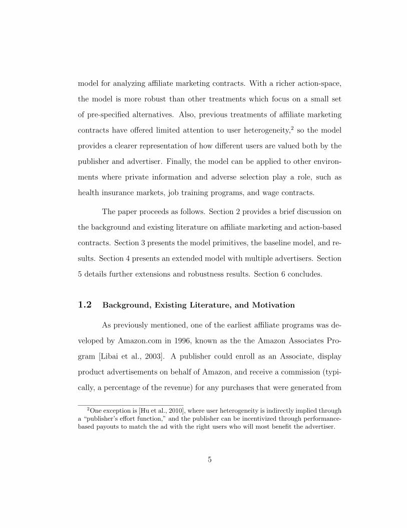
This probability is also known as a conversion rate. Consistent with

the marketing “funnel,” any action must occur at or before a sale, and, no sale

can be generated without the action being completed first:

Assumption 2. For any a, and any t,

i) pa(t) ≥ p(t), and

ii) P (S (t) = 1|A (t) = 0) = 0.

Figure 2a demonstrates this user path through a sequence of different

actions. What is important to note is that the post-action probability of sale

p(t)/pa(t) is larger if the action occurs “deeper” in the funnel, meaning that the

advertiser can achieve a better post-action success rate if leads are acquired

closer to the point of sale, and vice versa. This notion is better illustrated

through the joint action-sale probability distribution:

A(t), S(t) 1 0

1 p(t) pa(t)− p(t)0 0 1− pa(t)

An impression is a special case where pa (t) = 1; that is, the action (a

page view) is always taken. This action represents the beginning of the funnel,

since no user actions can be observed before the user arrives at the publisher’s

website. Because impressions happen automatically, there is no information

obtained through it, and so the posterior probability of sale is the same as the

prior, P (S(t) = 1|A(t) = 1) = P (S(t) = 1) = p(t). On the other end of the

spectrum is the final sale, which is a special (and redundant) action, where

14

pa(t) = p(t), and so P (S(t) = 1|A(t) = 1) = 1. Consistent with the funnel,

any other action must exhibit a conversion rate between these two extremes.

Assumption 3. For any action a, for any t, pa(t) ∈ [p(t), 1].

In the “funnel” model, actions are ordered based on their conversion

rate. This provides a convenient classification of actions, equally based on the

frequency of their occurrence, how “deep” the user is into the funnel, and the

corresponding post-action sale-probability p (t) /pa (t). Moreover, actions are

characterized not just on their conversion rate for a given t, but also how the

conversion rate varies across t.

Definition 1.3.3. The mapping between types and conversion rates is referred

to as the action-profile, pa : T → [0, 1].

Next, we define the set of conceivable action-profiles. Any action-profile

is conceivable so long as Assumption 3 holds.

Definition 1.3.4. The set of all conceivable action-profiles is P = {pa(t) :

∀t, p(t) ≤ pa(t) ≤ 1}.

Figure 2b shows the relationship between t, p (t), and P, along with

generic action-profiles. Next, we define the action space. The space of all

possible actions is denoted A. A key motivation of the model is that many

action choices are possible. The model will assume that A is so large that any

action profile in P is achievable.

15

Assumption 4. For any h (t) ∈ P, ∃a ∈ A such that pa (t) = h (t).

The richness ofA is one major innovation of this model, as it generalizes

the action-space from which advertisers can choose in formulating contracts.

A is infinite, and large enough that uncountably infinite action-profiles can be

achieved, with no restrictions on their shape other than Assumption 3. For

example, action profiles need not be monotone, continuous, or differentiable.

Assumption 4 simply states that there exists a large enough set of actions such

that any action-profile pa (t) can be achieved, so long as p (t) ≤ pa (t) ≤ 1 for

all t.

Lastly, the contract space is the Cartesian product R+ × A, and a

contract is a single point in this space, consisting of one action and one price.

In words, the contract determines that the publisher is paid the contract price

each time a user completes the specified action. The action-profile determines

how often that action will occur for each type.

Definition 1.3.5. A contract, denoted C = (c, a) ∈ R+ ×A, establishes that

the advertiser must pay a cost, c, for each user-type t whenever A (t) = 1.

It is assumed that the sale-probabilities and action-profile are known

by both parties when the contract is offered; thus, the baseline model does

not formally incorporate “learning” by either side. Moreover, the contract

is binding for the entire period, and each side is assumed to comply with

the terms of the contract, thereby eliminating any motivations for fraud. In

16

Section 5, the model will be extended to relax these assumptions. To conclude,

the model’s two main innovations are:

1. the existence of user heterogeneity as characterized by types t ∈ [0, 1]

with varying sale-probabilities p(t), and

2. the generalized action space A, from which advertisers can choose when

devising affiliate marketing contracts.

The baseline model to follow represents a sequential one-shot game between

advertiser and publisher. Contracts are offered from the advertiser to the

publisher in advance of a fixed period of time. The publisher then decides to

which user-types to show the advertisement. The analysis begins with solving

for the publisher’s best-response to a specified contract offered.

1.3.2 Publisher’s Problem

The publisher is a risk-neutral profit maximizer. For each user-type,

the publisher must decide whether to display the advertiser’s advertisement,

or some other alternative. For each type, the payout from the alternative has

a known, expected value of r(t). Qualitatively, r (t) might represent an offer

from a competing advertiser, or perhaps the opportunity cost of distracting

the user away from the publisher’s content.

Definition 1.3.6. The publisher must consider the choice function: v(t) :

T → {0, 1}, where v(t) = 1 if the publisher chooses the advertiser’s ad for

type t, and v(t) = 0 if the publisher chooses the alternative.

17

The publisher’s expected profit, as a function of the choice function

v(t) and contract C = (c, a), is:

E [ΠP (C, v)] =

∫

t

(v(t) · c · pa (t) + (1− v(t)) r (t)) dt (1.1)

Define the set of all mappings from T → {0, 1} as V . For an offered

contract, the publisher’s problem is:

maxv∈V

E [ΠP (C, v)] (1.2)

Solution

For any type t given to the advertiser, the per-view revenue, or expected payout

for the publisher is c×pa (t). The following definition establishes ma (t), which

will be a key object throughout the rest of the paper, and will be referenced

in succeeding propositions and solutions.

Definition 1.3.7. Define ma (t) = r(t)pa(t)

. This is the contract price which, for

a given action a, pays out r (t) in expectation for type t.

It is straightforward to verify that ma (t) × pa (t) = r (t). This is the

price paid to the publisher (for a given t) such that the expected payout from

the advertiser matches the expected payout from the alternative. Any price

lower than ma (t) makes the advertiser’s contract strictly worse, while any

price higher than ma (t) makes the advertiser’s contract strictly better.

18

From the definition above, it is straightforward to show that the pub-

lisher will show the advertisement for type t if and only if c ≥ ma (t). There-

fore:

v∗(t) =

{1 if c ≥ ma (t)

0 if c < ma (t)

The firm’s expected profit function is:

E [ΠP (C)] =

∫

t

max {pa(t) · c, r (t)} dt (1.3)

1.3.2.1 Targeting Properties of Action Profiles

At this stage, it is useful to demonstrate how the publisher’s optimal

response varies with the contract price that accompanies a given action. This

analysis will also serve to show the particular effectiveness of the action-profile

(pa(t)) in its ability to induce the publisher to show the ad only to a targeted

group of types. With a given action and corresponding action-profile, ma (t)

is fixed across t, and so the price level c will determine precisely which users

are shown the ad, and which users are shown the alternative.

Definition 1.3.8. For a given action a and contract price c, there exists a

target group of user-types, T : R+ × A → T , such that for t ∈ T (c, a),

v∗ (t) = 1, and for t /∈ T (c, a), v∗ (t) = 0.

19

Definition 1.3.9. From the publisher’s solution, T (c, a) = {t : c ≥ ma (t)}.

Proposition 1.3.1. For a fixed a, If ma (t) is weakly increasing over all t ∈ T ,

then there exists a cut-off type t(c) such that T (c, a) = [0, t(c)].

Proof. If ma (t) is weakly increasing, then if ∃ {t1, t2} ∈ T such that c =

ma (t1) = ma (t2), then ∀t ∈ [t1, t2], c = ma (t). Call tH = max {t : c = ma (t)}.

v∗ (t) = 1 if t ≤ tH and v∗ (t) = 0 if t > tH . If tH = ∅, then either v∗ (t) = 1 or

v∗ (t) = 0 ∀t. In all cases, v∗ (t) is monotonically decreasing in t. Therefore,

∃t :T (c, a) = [0, t].

T (c, a) foremostly defines the concept of a “target” user-population,

as in the set of users that the advertiser will ultimately reach. For a fixed

action-profile, the advertiser can only vary the price to induce the publisher

to show the advertisement to the desired type. Specifically, the advertiser

must set c = ma (t) in order to (at least) target type t. T (c, a) is weakly

increasing in c, which simply means that the advertiser reaches weakly more

users by increasing the contract price. Proposition 1 states a special case where

if ma (t) is increasing, then the target group is always a continuous interval

between t = 0 and some cut-off type t(c). This simply means that T (c, a)

always increases in t as well. This special case is a convenient framing of the

advertiser’s potential traffic pool, since the user-types are ordinally ranked

based on their sale-probabilities. Therefore, the advertiser can seek to target

20

the “best” user-types (as ranked by p(t)) and incrementally obtain lesser and

lesser types as seen fit.

Figure 3a-e illustrates this feature with various specifications of pa(t)

assuming a constant r (t) = r, along with corresponding graphs of T (c, a).

Notice how in some illustrations, T (c, a) is flat over some intervals. This

indicates that there are discontinuous jumps in pa(t) such that incremental

movements in c do not generate any new traffic. Also, notice how over intervals

where ma (t) is constant (in Figure 3a-e, since r(t) = r, this occurs when pa(t)

is constant), T (c, a) exhibits discontinuous jumps. This is because, to the

publisher, all types with the same pa(t) are identical from a revenue standpoint,

so they will always either be shown or not shown the ad in unison. Put another

way, if pa(t) = pa(t′) then v(t) = v(t′). Therefore, (t, t′) cannot be separated

with this particular action-profile.

Proposition 1.3.2. For a given a and pa(t), define:

T (κ) = {t ∈ T : ma (t) = κ ∈ R++}.

∀c, either T (c, a) ∩ T (κ) = T (κ) or T (c, a) ∩ T (κ) = ∅.

Proof. For all t, t′ ∈ T (κ), ma (t) = ma (t′), therefore, v(t) = v(t′). Therefore,

the targeted population will either include both types or none.

This speaks to the power of the action-profile as an instrument to tar-

get population types. For the advertiser, if a subset of types all have the same

21

conversion rate (relative to the publisher’s reservation pay-out), then subsets

within this subset cannot be separately targeted with that action profile. If

the action-profile specifies them as identical to the publisher, they cannot be

cleanly separated and must be either bought all together or foregone com-

pletely. This presents a problem to the advertiser, who may be interested in

filtering in and filtering out user types in precise detail.

Corollary 1.3.3. If ma (t) is increasing over all t ∈ T , and if ∃[t, t] ⊆ T

such that ∀t, t′ ∈ [t, t],ma (t) = ma (t′), then any t ∈ [t, t) cannot be a cut-off

type t(c) for any c. In the case where r(t) = r and for the impression action,

characterized pa(t) = 1, no t ∈ (0, 1) can be a cut-off type t(c) for any c.

In the special case where ma (t) is weakly increasing, if the advertiser

wishes to cleanly separate the user-types based on their value (high-revenue t’s

are shown the ad, while low-revenue t’s are not), this corollary demonstrates

that it would be impossible to do so if the action-profile specifies them as iden-

tical to the publisher. Moreover, in the particular case where the publisher’s

alternative pay-out is constant across types (r(t) = r) and the particular ac-

tion being considered is the impression (where pa(t) = 1), the advertiser has

no choice but to either target the whole population or none of it; there is no

ability to separate out any subsets of the user-types.

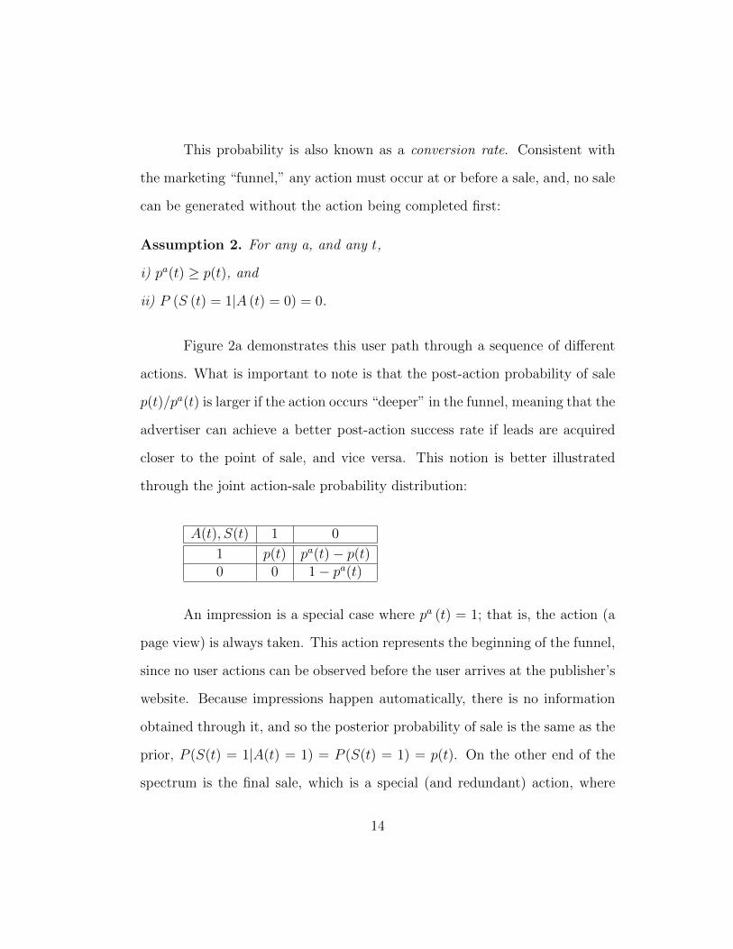
Observe Figure 4 to demonstrate, following Example A from Section

2. In this example, men (80%) are much more likely to generate a sale than

women (10%). However, using an impression-based contract the advertiser can

22

either target both men and women (by setting c ≥ r) or neither (by setting

c < r). This may not be optimal, particularly if it is not profitable to pay

the publisher to promote the ad to women. However, using the click-action,

because men (90%) are more likely to click than women (60%), the advertiser

can target men exclusively by setting r/0.9 ≤ c < r/0.6.

Even though the advertiser has to pay more per-click than per-impression

(since r (t) /pa (t) is higher than r (t)), the advertiser is still better off because

i) they have to pay for less clicks to generate the same number of sales, and ii)

importantly, they do not buy as many leads which ultimately will not produce

a sale. It is the ability to separate good types from bad that becomes the

primary concern for advertiser. The results above suggest that in many cases,

clean separation cannot occur if the action-profile does not conform to a shape

which makes separation possible. The contract price c can increase or decrease

traffic, but is limited in its ability to target particular user-types, which de-

pending on how p(t) varies, can be of a paramount importance. The contract

price is a blunt instrument in that regard, suggesting the advertiser can bet-

ter target desired user-types by manipulating the action-profile instead. The

following section will detail how the advertiser optimally chooses the contract

offered.

1.3.3 Advertiser’s Problem

The advertiser is also a risk-neutral profit-maximizer, and stands to

make π in profit from each sale. For a given contract, the advertiser generates

23

sales from whatever users are sent over from the advertiser, while only having

to pay the contract price for the users who complete the contract’s specified

action. However, the advertiser cannot distinguish the user types as they come

in, and so does not have complete control over which user types are completing

the action and thus generating expenses. As previewed by the previous section,

the advertiser has a three-stage problem in constructing a contract:

1. To determine which user-types to target,

2. To choose an action that effectively separates those desired users from

the undesired, and then,

3. To set a contract price that minimizes the total expenditure to acquire

those users.

For a given contract, and the publisher’s optimal response, the advertiser’s

expected profit function is:

E [ΠAd (C)] =

∫

t

[1 (t ∈ T (c, a)) (πp(t)− c · pa(t))] dt (1.4)

The advertiser’s problem is to choose a contract in order to maximize

expected profit:

E [ΠAd] = maxC∈A×R+

E [ΠAd(C)] (1.5)

Solution

24

The solution will begin by solving the three-fold problem in reverse.

Proposition 1.3.4. Given an action a with pa (t), suppose the advertiser must

acquire at least type t. Then, the optimal contract price is c∗ = ma (t).

Proof. Any c ≥ ma (t) successfully targets the user type. Assume c∗ > ma (t).

The advertiser can lower c∗ a small ε such that c − ε > ma (t). The type is

still targeted, but now costs are lower and therefore profit is higher. Thus, c∗

cannot be optimal.

Section 3.2 discussed that the publisher only shows the ad to a par-

ticular type t if c ≥ ma (t). Therefore, the advertiser, for each targeted

type t, will only pay the minimum per-type cost of r (t) by setting c so that

c× pa (t) = r (t).

Proposition 1.3.5. Given a set of targeted user types T , all contracts:

C (T ) = {(c, a) : (∀t ∈ T , c ≥ ma (t)) ∧ (∀t /∈ T , c < ma (t))}

will result in v∗ (t) = 1 (t ∈ T ).

Proof. Follows directly from the Publisher’s solution.

Leveraged with the action-spaceA, the advertiser can find the necessary

pa (t) to adjust which types see the ad and which do not. This is because for a

given c, the advertiser can adjust pa(t) such that all the targeted types exhibit

25

c ≥ ma (t), and all other types exhibit c < ma (t), thereby ensuring that the

publisher only promotes the ad to the types that the advertiser wishes to

target. Putting together Propositions 3 and 4, the solution is achieved:

• T ∗ = {t : πp(t)− r (t) ≥ 0}.

• C∗ (T ∗) = {(c, a) : (∀t ∈ T ∗, c = ma (t)) ∧ (∀t /∈ T ∗, c < ma (t))}.

• E [ΠAd] =∫t[1 (t ∈ T ∗) (πp(t)− r(t))] dt.

The optimal contract design also allows the advertiser to perfectly separate

the traffic population so that only the desired user-types are acquired, while

minimizing the expenses paid to reach those types (r(t)). Since the per-view

cost of r (t) can always be achieved, the advertiser chooses to target all users

such that πp(t) ≥ r (t).

1.3.4 Analysis

The solution to the advertiser’s problem presents three interesting con-

clusions. First, the contract’s action profile is a much more precise instrument

in determining which user-types are targeted and which are not. As shown in

Figure 3, moving the contract price c can result in large jumps in traffic or

nothing at all; however, finely tuning the action-profile can precisely exclude

the undesired user-types from the desired types. This speaks to the emphasis

on “creative” testing and other layout/design experimenting, which allows the

advertiser to hone their ability to make these incremental adjustments.

26

Second, aside from distinguishing the targeted types from the rest, the

action-profile can be chosen so that the advertiser only has to pay r (t) (and

no more) on a per-view basis for the user-traffic that is acquired. This is

achieved by selecting pa (t) such that ma (t) is constant across all the targeted

user-types. By doing so, the advertiser can offer the contract price c = ma (t),

resulting in paying the per-view price of r (t) for all targeted types. This is an

optimal result since r (t) is the minimum expected payout that still induces

the publisher to promote the advertisement to that type. Since πp (t) ≥ r (t)

for all types in the targeted set, per-type (expected) profits are always weakly

positive. Figure 5 demonstrates the profit scenarios for Example A. In the

examples, r (t) = r = $6 and π = $24. At these levels, only men are optimally

targeted because $24 · 0.9 > $6 and $24 · 0.1 < $6. Using the impression

action, the advertiser cannot exclusively target men, and so maximum profits

are lower than what can be achieved using the click-action. Note that for

both actions, the maximum profit point occurs when c = ma (t); any higher c

results in lower profits, either because i) the advertiser is obtaining user-types

that are not profitable, or ii) the advertiser is unnecessarily paying too much

in per-view costs.

Finally, the results above suggests a largely unintuitive result, that

contracts based on more informative actions (e.g. actions with an action-profile

that is small in magnitude, like in PPS contracts) are not always optimal.

This is because if the action profile pa(t) is low (ma (t) is high) for some t,

the advertiser must set a higher contract price c to target that type. That

27

higher price, however, has to be paid across all completed actions, including

those types who have a higher pa(t) (lower ma (t)), thereby increasing the costs

associated with these types. Therefore, it is optimal for the advertiser to choose

an action such that ma (t) is constant across all targeted types, regardless

of how informative the action may be. Take Figure 6a, which presents the

same illustration as Figure 5 except that p (Women) = 0.3. In this scenario,

targeting both men and women is profitable. Using the impression action, the

advertiser can achieve maximum profits by setting the contract price c = $6.

However, using the click-action, the advertiser must set c = mc (W ) = $10

to target both men and women. In doing so, the advertiser now must pays

$10 · 0.9 = $9 in per-view costs for men, higher than the $6 reservation price.

Thus, total profits are lower using the click action than the impression action,

even though clicks are more informative. This occurs because, in this special

case, the click action-profile (which varies across t) results in a varying ma (t)

across the targeted set of user types, while the impression action profile does

not.

Lastly, Figure 6b demonstrates that even PPS contracts will not be

optimal generally. Figure 6b takes the same illustration as Figure 6a, but

now assumes r (Women) = $5, while r (Men) = $6. It is still the case that

T ∗ = {Men,Women}, but for impressions, clicks, and even sales, ma (Men) 6=

ma (Women). Thus, none of these actions can be optimal. Instead, another

action would be required, such that ma∗ (Men) = ma∗ (Women).

The model results corroborate several stylized facts about the industry.

28

First, they help to explain why CPM contracts are so rare, and why the affil-

iate marketing industry was quick to move away from them. Many publishers

are not sourced with alternative options for every user-type which visits their

site, and so it is likely that they have a uniform alternative (r (t) = r) at hand

when considering an advertiser’s contract. In this case, a CPM contract can

only be evaluated against all user types lumped together. As an advertiser,

this often presents an unsatisfactory menu of options, as they are forced to

either forego profitable leads or be forced to buy unprofitable ones. When

launched, Google’s Adwords platform quickly sprung to dominance in large

part because the click, as opposed to the impression, was much more effective

at screening user-types in a profit-increasing way. Secondly, these results help

to explain why PPS contracts do not dominate the industry, even though they

are the most incentive-compatible for the publisher. Because the opportunity

cost of each type will vary in ways that do not match the sale-probabilities, a

larger set of alternative, more complex actions are required to both select and

price-discriminate the targeted set of users.

Discussion of Assumptions

The model’s essential results rest squarely on the assumption that the action

space A is large enough to allow the advertiser to choose any pa (t) ∈ P. Previ-

ous treatments have assumed only a small, finite number of actions from which

the advertiser may choose, which necessarily restricts the range of conversion

29

rates which might occur. On the other hand, in this model the definition of

P implies that the advertiser has the ability to set precise conversion rates for

all t. While these assumptions are an abstraction from reality, they represents

a reasonable approximation for two reasons. First, publishers and advertisers

have the ability to store and record vast amounts of user activity, where it be

page views, view duration, or information submission. Moreover, as data stor-

age becomes cheaper and more sophisticated, this set of actions continues to

grow. Secondly, the advertiser has many other levers with which to fine-tune

action conversion rates, including the text, graphics, display of the ad, and the

design and layout of the advertiser’s webpage. On the advertisement itself, ad-

vertisers can attract or detract users with varying degrees of aggressive text, or

“creative” [Zhu and Wilbur, 2011]. Similarly, the advertisement’s website can

be laid out to promote or dissuade users from completing the desired action.

With these tools at the advertiser’s disposal, it seems reasonable to assume

that a specified conversion rate may be reasonably achieved.

In practice, if an advertiser does not have this capability, then they

face a variant of a monopolist’s problem. In this scenario, the advertiser will

suffer some profit loss, either by foregoing types that would be profitable if

the cost were r (t), or, paying expenses greater than r (t) for targeted types.

To further illustrate, consider an arbitrary action such that i) ma (t) is strictly

increasing, and ii) p (t) − r (t) is decreasing. These attributes ensure ∃c such

that T (c, a) = [0, t] for any t, and T ∗ = [0, t] for some t.

Assume a fully differentiable action profile, and consider the problem

30

of choosing the optimal target population given this profile. We have the

following objective function:

maxt∈T

∫ t

0

(p(t)π −ma

(t)· pa(t)

)dt (1.6)

The expression ma(t)

replaces c(t)

according to Proposition 3. Taking

the derivative with respect to t, and observing first-order conditions, we obtain:

p(t)π − ∂(ma(t))

∂t

∫ t

0

pa (t) dt−ma(t)pa(t) = 0

Call∫ t

0pa (t) dt = Fa

(t).

p(t)π − r(t)− ∂

(ma(t))

∂tFa(t) = 0

p(t)π = r(t)

+∂(ma(t))

∂tFa(t)

The left-hand side represents the marginal revenue associated with the

marginal type at the optimum t. The right-hand side represents the marginal

costs associated with marginal type t. This includes the marginal costs of type

t alone (r(t)), plus, the marginal increase in the contract price

(∂(ma(t))/∂t)

which must be paid across all the preceding types Fa(t). This predicament

is analogous to a monopolist who, when lowering price to increase quan-

tity demanded, must lower prices for all units, not just the marginal unit.

This predicament occurs because the monopolist cannot distinguish consumer

31

types (based on their willingness to pay), and thus cannot effectively price-

discriminate. Similarly, the advertiser cannot distinguish the publisher’s user

types. However, unlike a monopolist, the advertiser has two levers to adjust:

price and action. By holding the contract price c constant, and increasing

pa(t)

such that ma(t)

decreases, the advertiser can devise an action profile

such that the marginal type can be obtained without increasing costs paid for

all other types. Effectively, the advertiser can price-discriminate each type

by varying pa (t). For the optimal contract, ma(t)

is constant ∀t ∈ T ∗ and

so ∂(ma(t))/∂t = 0, ensuring that marginal costs remain at r (t). Figure

7a-b shows this dynamic in the standard demand-supply framework. Similar

to monopolist markets, the advertiser ends up with total sales and total profit

lower than what would be achieved with perfect price discrimination.

These arguments demonstrate the increased flexibility the advertisers

achieve by having the choice of both the action and price when decided on

a contract. The more actions that the advertiser has in their choice set, the

more likely they are to find the optimal action profile which both selects and

price-discriminates the desired set of users.

1.3.5 Contracts as risk-sharing agreements

The results of the previous section may suggest that all action profiles

are equivalent so long as they i) successfully separate the targeted users from

the rest, and ii) are constructed so expected payouts always equal r(t). For a

risk-neutral advertiser, that is correct, as there exists, for a given t, infinitely

32

many (c, a) such that c = ma (t). To illustrate,

Proposition 1.3.6. If a contract (c, a) ∈ C∗ (T ∗), and if there exists another

action a such that(pa (t) ∈ P

)∧(pa (t) = βpa (t)

), then ∃c : (c, a) ∈ C∗ (T ∗).

Proof. Suggest c = cβ. Then c·pa (t) = c∗·pa∗ (t). If c = ma (t), then c = ma (t),

and if c < ma (t), then c < ma (t). Therefore, (c, a) ∈ C∗ (T ∗).

To explain, for a given optimal action profile pa (t), all positive scalar

multiples of pa (t) are also optimal, given that they exist in the action space P.

This is because the contract price c will respond in kind to keep c ·pa (t) = r (t)

∀t ∈ T ∗.

However, that is not to say that advertisers are completely indifferent

to the information content of the action profiles in this set.4 For example,

it is observed in the industry that many contracts exist which require deeply

informative actions. Examples include 2-3 page registrations, or even price-

per-sale contracts. One reason that advertisers may prefer more informative

actions to less informative ones may be the desire to exchange risk exposure.

Although expected profits are equal amongst all contracts in the optimal set,

the return-on-investment (ROI), or the ratio of profits to costs, will vary de-

pending on the information content of the action profile. ROI is a key business

4To refresh, pa1 (t) < pa2(t) means pa1 (t) is a more informative action than pa2 (t);pa (t) = p(t) is the most informative action possible, as it renders the post-action probabilityof sale exactly equal to one.

33

metric for all advertisers, and the advertiser may seek more or less informative

user actions depending on the advertiser’s risk aversion to variable returns.

To illustrate, it can be shown that as information content of the action

profile increases (that is, as pa(t) decreases from 1 to p(t)), the variance of ROI

is strictly increasing for publishers, while strictly decreasing for advertisers.

Proposition 1.3.7. Consider a targeted population T ∗ = [0, t], and the set

of optimal contracts C∗ (T ∗). If {(c1, a1) , (c2, a2)} ∈ C∗ (T ∗), and pa1 (t) <

pa2 (t) ∀t, then

1. V ar (ROIAd(C1)) < V ar (ROIAd(C2)), and

2. V ar (ROIP (C1)) > V ar (ROIP (C2)).

Proof. Consider a single t ∈ T ∗, and call the return on investment for this

type ROIAd (t, C).

E [ROIAd(t, C)] =πp(t)− cpa(t)

cpa(t)=π

c

p (t)

pa (t)− 1

ROI is simply a Bernoulli trial with parameter p(t)pa(t)

, multiplied by πc.

Var [ROIAd(t, C)] =(πc

)2 p (t)

pa (t)

(1− p (t)

pa (t)

)

Substitute in: c = ma (t) = r(t)pa(t)

per Proposition 3:

Var [ROIAd(t, C)] =

π(

r(t)pa(t)

)

2

p (t)

pa (t)

(1− p (t)

pa (t)

)=(πr

)2

p (t) (pa (t)− p (t))

34

Thus, if pa1 (t) < pa2 (t), then V ar (ROIAd(t, C1)) < V ar (ROIAd(t, C2)).

Since the Bernoulli trial parameter p(t)pa(t)

are unaffiliated across t ∈ T ∗, V ar (ROIAd(C1)) <

V ar (ROIAd(C2)). As the action profile gets closer to the sale function – ef-

fectively, increasing the post-action probability of sale – the advertiser realizes

less risk around expected return on investment. In the special case where the

pa (t) = p(t), variance is zero.

In the same analysis for publishers, where ROI is considered for just

the portion of traffic driven to the advertiser:

E [ROIP (t, C)] =cpa (t)

r (t)

Var [ROIP (t, C)] =(cr

)2

pa (t) (1− pa (t)) =

(1

pa (t)

)2

pa (t) (1− pa (t)) =1

pa (t)−1

Thus, variance of the publisher’s ROI increases with decreases in pa (t). For

the impression-action (pa (t) = pa = 1), variance is zero, since the publisher

receives the contract price c with absolute certainty on a per-view basis.

This model assumes both the advertiser and publisher are risk-neutral agents,

and thus, do not have preferences over the set of optimal action profiles. How-

ever, perhaps an extension of this model might assume one or both risk-averse

parties who would exhibit strict preferences over the profiles which affected

the uncertainty around return-on-investment. In fact, when both parties are

risk-averse, there could exist a risk premium on top of the risk-neutral contract

price to compensate the publisher for increased uncertainty. Such extensions

35

are not addressed in this work, but seem to be relevant and interesting ques-

tions for future research.

1.4 Model with Multiple Advertisers

The previous section extensively detailed the baseline model with one

publisher and one advertiser. Another model of interest, particularly to large

publishers who simultaneously negotiate with many advertisers, features one

publisher and many advertisers competing for the same page-space. Such a

scenario currently occurs with large search-companies like Google and Yahoo!,

only in a specialized format, namely where the action profile is restricted to

click only (with heavily regulated copy requirements) and where advertisers

must submit to a generalized second price auction. In this section, the baseline

model is extended to include multiple advertisers, so that each advertiser must

consider competing offers when constructing their own contracts.

Before a formal presentation of each agent’s problem, the terminology of

earnings-per-view (EPV) is introduced. EPV for type t is defined as epv (t) =

c · pa(t), and provides a short-hand description of the publisher’s expected

per-view revenue from a given contract. For reference, in the previous section,

the advertiser optimally structured the action profile so that epv (t) = r (t)

∀t ∈ T ∗. For the advertiser, epv (t) represents per-view expenses associated

with type t.

The model primitives are the same as before, with the extension that

there exists n ≥ 2 advertisers, which in the notation will be indexed by i.

36

As before, the publisher allocates each user type to the alternative with the

highest epv (t). In the baseline model, there were two alternatives: the ad-

vertiser’s contract or a reservation r (t). In the extension, the alternatives are

the offered contracts from all advertisers. Therefore, if multiple optimal con-

tracts exist for type t, any convex combination of those contracts will result

in maximum expected profit for the publisher. To standardize the allocation

between multiple competing contracts, this model extension assumes that if

the publisher is indifferent between more than one contract for type t, then

the publisher will split the user-traffic equally across each contract. Consider

vi(t) : T → [0, 1] the decision to offer some percentage between 0 and 1 of

traffic-type t to advertiser i. The publisher’s problem, formally stated given

an array of contracts {Ci}ni=1 is:

E [ΠP ({Ci}ni=1)] = max{vi}ni=1∈Vn

∫

t

(n∑

i=1

vi(t) · epvi (t))dt (1.7)

Denote epv (t) = max {{epvi (t)}ni=1}. Analogous to the baseline model,

the publisher’s solution is:

v∗i (t) =1 (epvi (t) = epv (t))

|argmax {epv (t)} | (1.8)

The advertiser’s problem, still contracting with just one publisher, remains

the same:

E[ΠAd(i)

]= max

Ci∈R+×Ai

{∫

t

v∗i (t) (pi(t)πi − epvi (t)) dt}

(1.9)

37

The model extension represents a modified case of Bertrand price competition,

with two main features. First, the competing firms are not homogenous; they

sell different products and thus have heterogenous valuations for each type t.

Second, as opposed to a deterministic unit price, the price competition takes

place in the space of expected per-view prices, taking into account a spectrum

of action profiles. Similar to the baseline model, note that for any contract,

the contract price ci is constant across t, while the action-profile pai (t) may

vary. Any precise manipulation of epv (t) must occur through variation in the

action profile, as the contract price will simply raise or lower epv (t) in a similar

fashion across all types, and therefore is a blunter instrument to maneuver.

Holding a contract price ci fixed, any epvi (t) greater than ci · pi(t) can be

achieved through varying pai (t).

Any advertiser i, when evaluating the possibility of targeting type t,

must only take into account the highest epv (t) being offered from all other

advertisers, denoted epv−it. Analogous to standard Bertrand competitions,

and assuming a minimum incremental adjustment of ε, the following best

response functions (in terms of epvi (t)) are presented:

BRi

(t, epv−i (t)

)=

{[0, pi (t) πi] if epv−i (t) > pi (t)πi

epv−i (t) + ε otherwise

For a given type t, an advertiser i can structure the pai (t) such that epvi (t)

just beats the epv(t) of the closest competitor, assuming it is still profitable

to obtain traffic at that expected per-view price. Given the best response

functions for all advertisers, the following “limit pricing” result is achieved:

38

Solution

Denote E [πi (t)] = pi (t) · πi.

• epv∗ (t) = E[π(n−1) (t)

]. For any type t, the maximum epv (t) offered,

and the publisher’s expected pre-view revenue, equals the second highest

expected sales revenue from all advertisers. The advertiser with the

highest expected sales revenue need only bid equal to the second highest

to successfully target type t. All other advertisers do not profit off type t,

either because they choose not to compete for that user type, or because

the price at which they must offer epv (t) equals their expected sales

revenue.

• T ∗i = {t : E [πi (t)] ≥ epv∗ (t)}.

C∗i (T ∗i ) = {(ci, ai) : (∀t ∈ T ∗i , epvi (t) = epv (t)) ∧ (∀t /∈ T ∗i , epvi (t) < epv (t))}.

Each advertiser only targets the user types for which their expected sales

revenue is the highest.

• E [ΠP ] =∫tepv∗ (t) dt. The publisher earns the 2nd best expected sales

revenue for each t.

• E[ΠAd(i)

]=∫tv∗i (pi(t)πi − epv∗ (t)) dt. Each advertiser earns profits on

all t for which they have the strictly best expected sales revenue.

1.4.1 Discussion

The model with multiple advertisers presents several interesting con-

clusions, many of which flow naturally as extensions from the baseline model.

39

First, the multiple-advertising model provides some insight into the origins of

r (t) in the baseline model. The baseline, which allowed for only one advertiser,

meant that that advertiser was competing against an exogenous alternative for

the publisher. Little legwork was given to explain the existence or valuation

of r (t). In many ways, this was not central to the advertiser’s problem, since

the advertiser had to “beat” the alternative to obtain traffic, regardless of

where the alternative came from. However, in the multiple-advertiser model,

it is clear to see that this alternative comes about from price competition of

other advertisers, and in particular, r (t) represents the next-best contract (on

a revenue per-view basis) for type t. In this regard, r (t) = epv∗ (t).

This model also illuminates the advantage advertisers can gain by being

able to offer promotions to the publisher that are different than competitors.

Note that

if E [πi (t)] = π (t) ,∀i, then E[ΠAd(i)

]= 0,∀i.

If all advertisers are marketing the same products, then they have no

choice but to bid away all the expected-revenue (also referred to as the “sur-

plus”) from each type t. As a result, the publisher receives all the expected

surplus from all user types. However, positive profits can be achieved if the

advertiser promotes a product which, for at least one t, has a higher-expected

revenue than all other competitors. For those types, the advertiser only has to

offer a contract which pays the equivalent of the next-highest valuation, and so

can obtain some positive expected profits. In this case, the publisher receives

a less-than-full portion of the surplus for those types. Therefore, identifying

40

products and promotions which can outpace other competitors for at least

some subset of users becomes a key consideration for the advertiser.

Furthering this notion, it also is no longer the case that the advertiser

targets the “best” traffic, which in this model, are user types t which are

smaller in magnitude. The shape of epv∗ (t) is generated as the 2nd-best

per-view offer from all advertisers; however, this does not imply that each

advertiser will always be second, or for that matter, hold a constant ordinal

ranking across all type t. If it is the case that two advertisers exhibit profiles

of E [πi (t)] which intersect at least once, then there will exist intervals of

T where one advertiser will outpace the other in terms of expected revenue,

and vice versa. In particular, for some advertisers, positive profits will be

generated exclusively off of lower-quality traffic (as ranked by E [π (t)]) because

those types are the only ones in which they can outpace other advertisers and

acquire from the publisher. The user-allocation, e.g. which types go to which

advertiser, depends critically on the relative advertisers’ valuations, and for

some advertisers, lower-revenue types may be the most valuable to obtain.

To illustrate these insights, refer to Figure 8a, which depicts Example

A again, but now includes the existence of a second advertiser that is pro-

moting yoga classes. In the figure, the fantasy football advertiser has values

men-types at $7 and women-types $4, while the yoga class advertiser values

them at $5 and $6, respectively. Therefore, the valuation of yoga classes com-

pared to fantasy football is higher for women than for men. Accordingly, both

advertisers will submit contracts with per-view revenue equal to the minimum

41

valuation for each type. When a particular advertiser has a relative advan-

tage, they will gain positive profit on that type, and when that advertiser has

a relative disadvantage, they will earn zero profit. Both advertisers choose

this route because they would lose money if they bid for types above their own

valuation, and need only to match their competitor to attain types where they

hold the advantage. Based on these contracts, the publisher will optimally

choose to show the fantasy football ad on the men’s page, and the yoga class

ad on the women’s page. The yoga class advertiser achieves a positive profit

targeting women because of their relative advantage over the fantasy football

advertiser. In the end, all parties gain some positive profit. The publisher

receives payments from both advertisers, the fantasy football advertiser reaps

profits from sales generated by users on the men’s page, and the yoga class

advertiser reaps profits from sales generated by users on the women’s page.

Figure 8b offers a more generic illustration of this occurrence, again as-

suming just two advertisers. Because E [π1 (t)] and E [π2 (t)] intersect once and

only once, the user-spectrum is cleanly split between the two, with each ad-

vertiser obtaining the interval of types where their valuation is highest. Both

advertisers make positive profits with their respective targeted types, since

they only have to offer contracts commensurate with the next best option.

The publisher receives the expected revenue consistent with the next-best op-

tion for all types t, which in general will be smaller (as a portion of the total

surplus) as the gap in expected revenue between advertisers 1 and 2 widens.

These two examples demonstrate how matches are formed in the affiliate mar-

42

keting industry. First, clearly an advertiser must be promoting a product

which has some relevance to the publisher’s user population; if not, then the

valuation profile E [πi (t)] would be so small (or null) that the advertiser would

have no ability to compete for user traffic. On the other hand, if the adver-

tiser is promoting a product which is highly correlated or closely aligned with

their competitors, the level of achievable profit will be diminished as well. In

the most extreme case, if an advertiser pitches the exact same product as a

competitor (or more generally, a product with an identical valuation profile

E [πi (t)]), then they stand to achieve zero profit. Therefore, the model sug-

gests that the best, most stable matches occur when an advertiser can promote

a product that is differentiated from its competitors yet still highly relevant

to the publisher.

Lastly, this analysis illuminates once again the advertisers’ necessity

of having an expanded choice set of action profiles when delivering contracts.

Recall that Google’s and other search engines’ generalized second price auc-

tions rank each advertiser buy expected per-view revenue (click-through rate

multiplied by bid), and each ad placement is awarded at the per-view cost

of the next highest bidder.5 However, the search engines commonly allow

just CPC advertising, meaning that each advertiser must compete using the

click-action. This implies that, unless the advertiser can manipulate the click-

through rate to precisely match their valuation of each type, then they will

5This outcome is almost identical to the one achieved in the Bertrand competition de-tailed above, where the advertiser who wins a particular user type need only bid the valuationof the 2nd best advertiser.

43

be constrained in how they can compete, and how they can minimize costs.

Refer again to Figure 8a. The optimal contract in this example requires that

ma∗ (Men) = ma∗ (Women). If constrained to only clicks, each advertiser

must manipulate their ad such that the click-through probabilities match this

profile. If this cannot be precisely done, then the advertisers will be at some

loss. If the click-through rate is too high for a given type, the advertisers either

bids more than is needed to secure the user type, or bids over their own valu-

ation. If the click-through rate is too low for a given type, the advertiser is in

danger of being unable to win the desired user type. This example showcases

that the restriction to just one or a small set of actions when constructing

contracts means the advertiser may not be able to precisely target a desired

user population at the minimum price. Put another way, the more actions

that an advertiser has at their disposal, the better able they are to craft this

optimal action profile and contract.

In the real world, this insight reveals that advertisers’ ability to compete

for publishers’ ad space depends critically on their access to a wider and more

elaborate set of user actions. Case in point, suppose there exists two advertisers

with the same valuation profile E [π (t)]. A standard preconception may be

that these two advertisers are equally competitive, given they have the same

expected revenues for all types. However, suppose that one firm is much more

technologically savvy than the other, and has access to structure contracts

and much more detailed and finely-tuned user actions. In this case, the less-

savvy firm would be at a competitive loss, generally speaking, as they would

44

not possess the same ability to craft optimal contracts against the publisher’s

per-view reservation prices. Over time, the tech-savvy advertiser would win

out, as they would be able to generate more profit, despite having the same

exact valuation profile.

These arguments highlight both the complexity and the increased flex-

ibility of affiliate marketing contracts, and demonstrate why a rich set of con-

tractible actions is so critical to the advertiser. With a plethora of actions,

advertisers, competing against each other for publishers’ page-space, have an

increased ability to craft contracts that lower their expenses while selecting

out unprofitable user types. As the action set grows, advertisers can fine-tune

this procedure even further. This suggests that matches between an advertiser

and a publisher not only depend on a strong product alignment (differentiated

from competitors, relevant to users) but also on the advertiser’s technological

capability in selecting and crafting optimal action-profiles.

1.5 Model Extensions and Special Cases

The following section will detail several extensions and/or special cases

of the baseline model to implement various features that could be more rep-

resentative of real-world conditions for both publishers and advertisers.

1.5.1 Repeated Game with Default Option

This section presents a repeated-game framework, where the advertiser

has the option to default on payments owed to the publisher for marketing

45

services already received. One assumption of the baseline model was that if

a contract were accepted, it would be enforced by both parties. However, in

any one-shot game, there is no incentive for the advertiser to “make good” on

their payments. In a one-time game, once the advertiser receives the users sent

over from the publisher, the advertiser now has an incentive to default on the

payments owed. Moreover, this default decision may not occur immediately,

as many contracts in the affiliate marketing industry are “net 30,” meaning

a month’s worth of leads are invoiced at a time (typically at the end of the

month), and then the advertiser has another 30 days to settle the payment.

In such agreements, there is nontrivial payment risk borne by the publisher,

who can supply up to two month’s worth of leads without scheduled cash

compensation. Therefore, if the advertiser chooses to default, they may receive

up to two month’s of leads without ever having to pay for them. Also, aside

from just all-or-nothing payment, any action that occurs on the advertiser’s

website often cannot be independently observed by the publisher. Thus, the

advertiser also has the incentive to “scrub” the number actions generated, in

an attempt to cheat the publisher and lower costs.

The model will be extended into a repeated game setting, to analyze

how honest accounting and payments might be enforced. Consider the adver-

tiser’s and publisher’s problem over an infinite horizon. Within each period,

the advertiser must decide two things, i) the optimal contract to offer, and

ii) what portion of payments on which to make good once leads are received.

The publisher must decide whether to accept the advertiser’s contract, and

46

importantly, does not observe whether the advertiser has paid until the next

period. Therefore, there is always a one-period opportunity for advertiser to

shirk its costs. The timing of the game is as follows:

1. The advertiser offers a contract, C.

2. The publisher either accepts or rejects the contract, and offers leads in

accordance with that contract.

3. The advertiser decides what to pay for the generated leads.

Define the variable dj ∈ [0, 1] to be the portion of the payment the advertiser

will choose to pay. The publisher discounts profits in time period j (relative

to j = 0) by the discount factor βjP . The publisher’s problem is to maximize

expected discounted profits, taking into account payment risk:

max{vj}∞j=0

{∞∑

j=0

βjP

∫

t

(vj(t) · dj · cj · paj (t) + (1− vj(t)) r (t)) dt

}(1.10)

The advertisers discounts profits in time period j by βjAd. The ad-

vertiser’s problem is to jointly choose an optimal contract and a payment

probability:

maxCj∈R+×A,dj∈[0,1]

{∞∑

j=0

βjAd

∫

t

vj (t) (p(t)π − dj · cj · paj(t)) dt}

(1.11)

47

Solution

First note that, for both the advertiser and publisher, any contract price ci

with a less-than-one payment probability di < 1 is equivalent (in expectation)

to the contract price cidi

with probability payment equal to one. Intuitively,

if the advertiser defaults on 40% of the payment (d = 0.6), or the advertiser

lowers the contract price by 40%, these two acts result in the same bottom

line for the publisher.

Next, note that the advertiser will always choose to target the same

T ∗ in each period, and that T ∗ equals the optimal user-type interval obtained

in the single-period problem with no default. Recall that in that problem,

the advertiser chooses to target T ∗ = {t : p(t) ≥ r (t)}. For any nonzero

payment probability di > 0, it is never optimal to target any user-type where

p(t) < r (t). This is because the advertiser cannot select which types to make

good, only on whether to honor the whole invoice or not, and therefore there

is some nonzero probability of paying for traffic which will result in expected

loss.

Therefore, the advertiser’s problem reduces to a choice over whether to

default, holding the optimal contract fixed in each period. The single-period

game, repeated infinitely, can be written in normal form as follows:

Ad, P Accept Reject

Pay(∫

tv∗ (t) (p (t) π − r (t)) dt,

∫tr (t) dt

) (0,∫tr (t) dt

)

Default(∫

tv∗ (t) p (t)πdt,

∫t(1− v∗ (t)) r (t) dt

) (0,∫tr (t) dt

)

48

Equilibrium

It is clear to see that in the single-period setting, the unique perfect equilibrium

is (Reject,Default), since (Accept) is a weakly dominated strategy. However,

both parties are (weakly) better off, and the advertiser is strictly better off, by

cooperating. This amounts to a repeated prisoner’s dilemma, where a weakly

better out come can only be obtained through penal enforcement. The “grim

trigger” penal rule to enforce co-operation in the repeated game is presented.

1. For period j = 0, the publisher accepts.

2. j > 0, the publisher accepts if the advertiser pays in full in period j−1. If

advertiser defaults at all in period j−1, the publisher rejects for periods

j, j + 1, ....

3. The advertiser always pays if the publisher accepts.

Call π =∫ 1

0v∗ (t) p (t) πdt and r =

∫ 1

0v∗ (t) r (t) dt. The advertiser’s profits

under (Accept, Pay) are (π − r), and under (Accept,Default), π. Under the

publisher’s rule, the advertiser will decide to pay if:

π − r1− βAd

≥ π

r

π≤ βAd

49

π

r− 1 ≥ 1

βAd− 1

The “grim trigger” rule will enforce cooperation so long as return-on-

investment meets or exceeds the advertiser’s discount rate. Two main conclu-

sions arrive from this result. One, an advertiser with a high discount rate will

optimally choose to default, and simply “grab” the one-time profit boost asso-

ciated with shirking costs for one period. In the affiliate marketing industry,

this tends to occur with firms who are financially unstable, and face significant

liquidity strain to make good on their accounts receivable each month. These

types of advertiser’s quickly leave the industry, as their reputation for non-

payment makes it difficult to work with other publishers. Two, the matching

between advertisers and publishers must be such that the expected revenues

of the targeted user types sufficiently outpace the per-view price. The adver-

tiser is more likely to default if the profit margins (present and future) are

not large enough to incentivize the advertiser to enforce the contract in the

present in order to keep them. This suggests there are limits in the matches

between advertisers and publishers. Marginally profitable contracts are likely

to be rejected because the incentive to default is quite high.

1.5.2 Contracts with Learning

This model extension will assume that the advertiser or publisher does

not know the respective sale- and action-probabilities, and learn over time.

So far, the analysis has assumed that the sale function and a specified action-

50

profile is known, but in many cases, contracts are offered to new publishers

with whom p(t) and pa (t) cannot be known exactly, but can be estimated as

leads begin to accumulate. This extension will investigate how the advertiser

should design its contract to incorporate this uncertainty.

Note that the advertiser is interested in all user-types t such that p(t) ≥

r (t). Therefore, the advertiser is interested in identifying some confidence

interval for p(t), or alternatively, testing the null hypothesis that p(t) ≥ r (t).

The analysis begins by assuming that for a given user-space T , the ad-

vertiser has a prior distribution of the sale-probabilities for each t, denoted

µt(p(t)). That is, the advertiser has a subjective distribution over the pos-

sible values of p(t), which is itself a distribution over {0, 1}. Analogous to

the baseline model, if the advertiser can only offer one contract, and never

renegotiate, they will offer a contract which targets the relevant user-types

such that E [µt(p(t))] ≥ r (t). Also, for a given action-profile, there exists a

prior distribution, νt (pa (t)). Analogous to the baseline model, if the publisher

is only offered one contract, the publisher only promotes the ad to type t if

c = r(t)

E[νt(pa(t))].

In the framework presented below, the advertiser can observe the per-

formance of user-types in discrete intervals, and update their contract specifi-

cations for the next interval. In practice, most advertisers adopt some version

of this procedure, most notably by first offering a contract for a testing pe-

riod, then, offering a new, permanent contract with an updated distribution of

µt (p(t)). The testing period is used to acquire observations which update the

51

prior distributions, and allow for the new contract to be constructed with more

precision, leading to higher expected profits for both parties. This procedure

reveals that there exists a continuation value associated with each posterior

distribution. Call the publisher’s continuation value VP (νt (pa (t))) and the

advertiser’s continuation value VAd (νt (pa (t)) , µt (p (t))).

Let us denote each period by subscript j = 0, 1, 2, ..., and the distribu-

tions conditional on history through period j as µt (p(t)) |j and νt (pa (t)) |j,

respectively. The publisher’s problem in period j + 1 (and having observed

history through j) becomes:

E [ΠP (C) |j] = maxv∈V{∫

t

[v (t) (c · E [νt (pa (t)) |j]) + (1− v (t)) r (t)] dt+

VP (νt (pa (t)) |j + 1)} (1.12)

And the advertiser’s problem:

E [ΠAd|j] = maxC∈R+×A{∫tv∗ (t) (E [µt (p(t)) |dj] π − c · E [νt (pa (t)) |j]) dt+VAd (νt (pa (t)) , µt (p (t)) |j + 1)}

(1.13)

The publisher must make inferences on the true profile of pa (t), while

the advertiser must make inferences on both p(t) and pa (t), conditional on the

information obtained through interval j. This naturally requires using Bayes’

rule. Since the random variables S(t) and A (t) follow a binomial distribution

52

with parameters p(t) and pa (t), respectively, it is natural and algebraically

convenient to assume the prior distribution follows a beta distribution with

hyper-parameters (αt, βt) for µt (p (t)) and (at, bt) for νt (pa (t)). Under this

family of distributions, the prior and posterior distributions (after applying

Bayes’ rule) are of the same family, thus allowing for closed-form expressions

for the posterior distribution. Such families are called conjugate distributions,

and the beta distribution is a well-known example.

Lastly, the problem is somewhat complicated by the notion that if a

type t is not targeted, then neither the advertiser nor the publisher can attain

information about type t. This may be unsatisfactory if the prior distribution

for type t is especially disperse, such that additional information will lower the

variance of the posterior distribution dramatically. Both parties are interested

in constructing a binary decision for each type t – for the publisher, whether

to show the ad or not, for the advertiser, whether to target or not. The pub-

lisher, for each t, wishes to test the hypotheses c · pa (t) ≥ r (t), while the

advertiser wishes to test p (t) π ≥ r (t), as these inequalities determine each

party’s decision. Therefore, it becomes critical to allow for exploration of the

behavior of type t until a test with sufficiently small size can be rejected. The

analysis will assume each party adopts a test of this null hypothesis with size

γ, such that, each party will only make a final decision on each type t with

at least (1− γ) % confidence. This notion is similar to the “explore-exploit”

trade-off inherent in multi-armed bandit problems, for which many approxi-

mated solution strategies have been previously derived. The strategy below

53

will be a variant of epsilon-first strategy, except that the exploration phase

is dynamically determined based on the first rejection of the null hypotheses

Tran-Thanh et al. [2010].

Optimal Decisions Under Bayesian Learning

Assume that before the first period, j = 0, the advertiser has a prior distribu-

tion for each t, µt (p (t)) ∼ Beta (α0 (t) , β0 (t)), and the publisher has a prior

distribution for each t, νt (pa (t)) ∼ Beta(a0, b0). The following procedure de-

tails the optimal decisions for both publisher and advertiser at each interval,

as well as the posterior distribution generation which informs those decisions.

1. Re-arrange types in descending order based on the 1 − γ-percentile of

µt (p (t)) |j = 0, denoted q1−γ [µt (p (t)) |j = 0].

2. For the publisher , choose T ∗ = {t : q1−γ [πµt (p (t)) |j = 0] ≥ r (t)}.

All {t : q1−γ [πµt (p (t)) |j = 0] < r (t)} are not targeted.

3. The contract C∗ = (c∗, a∗) is offered such that ∀t ∈ T ∗, q1−γ [c∗ · νt (pa∗ (t)) |j = 0] =

r (t).

4. After period j = 1 is complete, the publisher and advertiser jointly

observe N1 (t) views and A1 (t) actions for each user-type t ∈ T ∗; the

advertiser also observes the number of sales S1 (t).

5. The publisher updates the prior distribution

(a0 (t) , b0 (t)) = (a0 (t) + A1 (t) , b0 (t) +N1 (t)− A1 (t)).

54

6. The advertiser updates the prior distribution

(α0 (t) , β0 (t)) = (α0 (t) + S1 (t) , β0 (t) +N1 (t)− S1 (t)).

7. Repeat steps 1-6 with prior distribution µt (p (t)) |j = 1, 2, ... and νt (pa (t)) |j =

1, 2, ....

As j → ∞, µt (p (t)) |j → p (t) and νt (pa (t)) |j → pa (t). Thus, the baseline

model can be characterized as the limiting-state of a model with learning.

1.5.3 Finite User-types

The baseline model assumed a spectrum of user-types; in reality, this

may be a strong assumption, given that it would entail the publisher and

advertiser being able to ascertain finely-tuned differences across users. Instead,

it may be more reasonable to assume a finite set of user-types. However, this is

no different that modeling p(t) as a k-step function, to construct k user-types.

That is, a sale function of:

p(t) =

p1 if t ≤ t1

p2 if t1 ≤ t ≤ t2

...

pk tk−1 ≤ t ≤ tk

Where p1 > p2 > ... > pk. Per Proposition 2, only k types can be identified

by the publisher or advertiser. All the results continue to hold, as this is a

special case of the more general model.

55

1.6 Conclusions, Limitations, and Future Work

The model presents several results, some which confirm the existing lit-

erature, and some which offer new and somewhat counterintuitive insights into

the optimal structure of affiliate marketing contracts. First, the action-profile’s

ability to raise the ex-post probability of sale and limit “wasteful” spending

is largely a non-issue. In fact, in some cases, actions which have higher ex-

post sale probabilities can be suboptimal if they do not precisely match the

publisher’s opportunity cost. Risk-neutral advertisers are largely indifferent

to the riskiness of an action-profile so long as per-view performance remains

the same. Rather, the benefits of an action-profile lie primarily in the ability

to separate user types into a targeted and non-targeted set of users. Actions

are utilized to target specific users exclusively, by inducing the publisher to

promote to desired users and not to promote to others. Therefore, impressions

are largely ineffective in this regard, and this rigidity may help to explain why

CPM contracts are rarely utilized. Moreover, the advertiser crafts an action

such that for each desired type, the advertiser pays the publisher the minimum

per-view amount needed to induce the publisher to agree. This speaks to the

dual nature of actions, both to separate the user traffic while also minimizing

expenses. When there are many different user types, each with varying worth

to both the advertiser and publisher, achieving both of these goals requires

a rich set of contractible actions. This main result offers a novel explanation

behind the diversity of action-based contracts in the industry.

In the extended model with multiple advertisers, advertisers must en-

56

gage in expected per-view Bertrand price competition, and the publisher enjoys

the added revenue associated with the limit pricing of their user types. As a

special case, if all advertisers sell the same product, the publisher earns the

advertisers’ entire sales revenue; on the other hand, an advertiser can only

earn positive profits if their per-view valuations are higher than all other com-

petitors for at least one user type. This suggests that the most competitive

advertisers will be ones who promote products that are differentiated from

others, while still be relevant and profitable within the user population. It

is also the case that some advertisers will explicitly and deliberately target

low-quality users if they have a relative advantage over those types. This may

help to explain why particular goods or services do well for some publishers

even if those goods or services are deemed inferior by a broad swath of other

publishers and traditional media. In sum, the model arrives at results which

offer profound insight on advertisers’ strategy and corroborate many stylized

facts about the online affiliate marketing industry.

This paper provides two contributions to the current literature on affili-

ate marketing contracts. First, the model provides a formal, general economic

treatment of the affiliate contract problem using microeconomic theory, by

specifying primitives on user behavior, and publisher and advertiser prefer-

ences. The development of a rich action-space allows for a broader analysis

of action-based contracts. Since the literature is largely rooted in analyzing

just two or three different alternatives, previous models cannot comment on

how a larger set of action affects firms in the industry. As the set of identi-

57

fiable user actions continues to grow, the generalized framework offered here

will prove to be more useful than models which assume only a small set of

pre-existing actions. Moreover, by introducing user heterogeneity and asym-

metric information, the model accounts for selection implications associated

with action-profile choices which have not yet been extensively analyzed. Sec-

ond, this paper offers a novel explanation on the diversity of actions used in

the affiliate marketing industry. To illustrate, advertisers with only a limited

set of actions with which to incorporate into a contract will be constrained in

their ability to perfectly match the publisher’s reservation prices for the user

types they wish to target, and therefore will suffer inefficiencies either in their

selection of users or in the prices they must pay to attain those users. Finally,

this framework can be applied to other environments with agent heterogeneity

and asymmetric information as well. Below are two examples:

EXAMPLE D: A firm is looking to hire from a heterogenous

pool of workers. Workers are of different types, t, which put

forth constant effort but produce varying output for the firm with

expected value, y (t). Meanwhile, each type has varying reser-

vation wages, r (t), and the firm wishes to hire all types such

that T ∗ = {t : y (t) ≥ r (t)}. However, the firm cannot distin-

guish worker types, so it must construct a performance-based con-

tract to target the right workers while also minimizing labor costs.

A contract based which pays a fixed amount, w, conditional on

an observable performance benchmark, B (t), such that ∀t /∈ T ∗,w · P (B(t) = 1) < r (t), and ∀t1, t2 ∈ T ∗, mB (t1) = mB (t2), will

58

effectively target the profitable workers while paying them no more

than r (t) in expectation.

EXAMPLE E: A university is recruiting students to enroll. Stu-

dents are of different types, t, with varying enrollment rates, e (t).

The university makes π in net revenue off of each enrollment. The

university contracts with recruiters who know the student types.

For the recruiters, each type has a different recruiting cost, r (t),

in terms of time and effort. The optimal contract offered by the

university to the recruiter will be based on an enrollment bench-

mark which occurs with probability pe (t), such that the recruiters

only recruit types T ∗ = {t : πe (t) ≥ r (t)} are only paid r (t) in

expectation.

As the examples illustrate, the modeling framework presented here is quite

robust to other environments where asymmetric information and adverse se-

lection play a role.

This model also comes with distinct limitations which could be en-

hanced with future work. For instance, the assumption that the choice of

action-profiles is infinite may be too broad, and so further results which can

identify optimal strategies over a general, but finite set of action profiles may

prove useful. For example, a treatment where action-profiles are finite, and the

advertiser must choose the profile which best matches the unconstrained profile

would be of interest, particularly as it relates to implementability. Secondly,

the featured model here was static, and represented a steady-state environment

59

where full valuations and action-profiles were known. Extending the model to

a dynamic setting, where agents must manage noisy information about these

primitives, financial risks, and relationship considerations with other partners,

would present a more realistic scenario as it pertains to this industry. Thirdly,

analyzing the predictions of this model empirically would also demonstrate

a valuable contribution. While aggregate data on affiliate marketing arrange-

ments are not abundant, there exist many large affiliate networks6 – exchanges

between publisher and advertisers – which may possess the volume of breadth

of data necessary to investigate advertisers’ strategy on a broad scale.

6Examples include Commission Junction and LinkShare.

60

1.7 List of Figures

UserUser visits

Publisher′s website...

Publisher’s Website

DisplayAdvertisement

Pay-per-impression

observesad...

Advertiser’s Website

clicksad...

PPCenters

Advertiser′swebsite...

takes“lead”action...

PPA

makespurchase

PPS

Figure 1: An illustration of the interactions between an internet

user, the publisher, and the advertiser. The publisher’s role is to

display the advertisement on behalf of the advertiser. The user

visits the publisher’s website, and then may or may not proceed

to engage the advertiser through the display ad. Depending on

the terms of the contract, the publisher receives payment from

the advertiser upon, among others, the display of the ad (pay-

per-impression), a user click of the ad (pay-per-click, or PPC), a

pre-specified user action which classifies the user as a lead (PPA),

or a user purchase (PPS).

61

user visits publisher’s site

impression occurs with prob. 1

user observes ad with prob pa11− pa1

$0

$0

clicks ad with prob pa2

pa11− pa2

pa1

$0

registers with prob pa3

pa21− pa3

pa2

actions 4 to n− 1

$0

purchases with prob ppan−11− p

pan−1

$π

Figure 2a: An illustration of the user “funnel” from an impression

to a sale, assuming n distinct, post-impression actions. In this

example, the user receives an impression of the ad with probability

one. Ex ante, the user can observe the ad with probability pa1 ,

click the ad with probability pa2 , register with the advertiser with

probability pa3 , and eventually purchase (the nTh. action) with

probability p. The probability of sale conditional on any action i is

ppai

, and must be weakly increasing in i. The “funnel” framework

mandates that all actions be completed sequentially, such that the

failure to complete any action results in a terminal advertiser payoff

of $0.

62

1

10User Types, t ∈ [0, 1]

p(t)

pa(t) = 1P

Figure 2b: An illustration of a generic sale-profile and various

action-profiles. The horizontal axis is the domain of t ∈ T = [0, 1],

and the vertical axis is the probability space over binary outcomes.

The grayed area is the space of all potential action-profiles, P. P

is bounded above by pa(t) = 1, which is an “impression,” and

bounded below by p(t), which is a sale.

63

(a)

1

10t

pa(t) = κ

1

0 c

T (c, a)

rκ

(b)

1

10t

pa(t)

1

0 c

T (c, a)

(c)

1

10t

pa(t)

1

0 c

T (c, a)

(d)

1

10t

pa(t)

1

0 c

T (c, a)

(e)

1

10t

pa(t)

1

0 c

T (c, a)

Figure 3a-e: An illustration of various specifications of pa(t) and

their corresponding T (c, a).

(a) The impression-based action, where pa(t) = κ, and T (c, a) = ∅∀c < r

κ, and T (c, a) = T ∀c ≥ r

κ.

(b) pa(t) has discrete jumps, but constant wherever continuous;

T (c, a) has a step-up shape.

(c) pa(t) is decreasing with discrete jumps; T (c, a) has periodic

plateaus but otherwise increasing.

(d) pa(t) is continuous, but constant over some intervals, in which

case T (c, a) has periodic jumps.

(e) pa(t) is continuous and strictly decreasing, in which case T (c, a)

is strictly increasing.

64

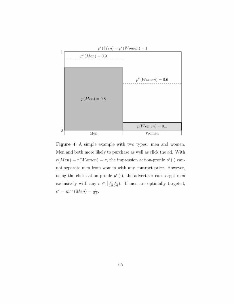
0

1

p(Men) = 0.8

p(Women) = 0.1

pc (Men) = 0.9

pc (Women) = 0.6

pi (Men) = pi (Women) = 1

Men Women

Figure 4: A simple example with two types: men and women.

Men and both more likely to purchase as well as click the ad. With

r(Men) = r(Women) = r, the impression action-profile pi (·) can-

not separate men from women with any contract price. However,

using the click action-profile pc (·), the advertiser can target men

exclusively with any c ∈ [ r0.9

r0.6

). If men are optimally targeted,

c∗ = mac (Men) = r0.9

.

65

0 c

$8

$− 2

r(M) = r(W ) = $6

π = $24

mi (M) = mi (W ) = $6

mc (M) mc (W )

Impression contract

Click contract

ExpectedProfits

Contract Price

Figure 5: An illustration of expected profits as a function of the

contract price c, for both the click and impression action-profiles.

With the impression contract, the advertiser can only target both

men and women, or neither. However, with r = $6 and π = $24,

targeting women is not profitable. With the click action, the adver-

tiser can target men exclusively, and optimally does so by setting

c∗ = mc (M) = $60.9

. The unprofitability of women is illustrated at

c = mc (W ) = $60.6

, where aggregate profit discontinuously drops as

women are included in the targeted set. By being able to target

men exclusively, the advertiser achieves higher profits ($6.66) than

would be achieved with impressions ($4.8) because the publisher

does not show women the ad.

66

0 c

$16

$− 4

r(M) = r(W ) = $6p(M) = 0.8 , p(W ) = 0.3pc(M) = 0.9 , pc(W ) = 0.6

mi (M) = mi (W ) = $6

mc (M) mc (W )

Impression contract

Click contract

ExpectedProfits

Contract Price

Figure 6a: An illustration of expected profits as a function of the

contract price c, for both the click and impression action-profile.

If p (Women) = 0.3, then T ∗ = {M,W}, and the impression,

not the click, is optimal. This is because with the click action,

mc (Men) < mc (Women), so the advertiser has to offer a higher

contract price (c = $10) to target women, resulting in higher per-

view costs for men. With the impression action, the advertiser can

pay per-view costs of $6, equal to r, to obtain both traffic types,

and so profits with the impression action are higher.

67

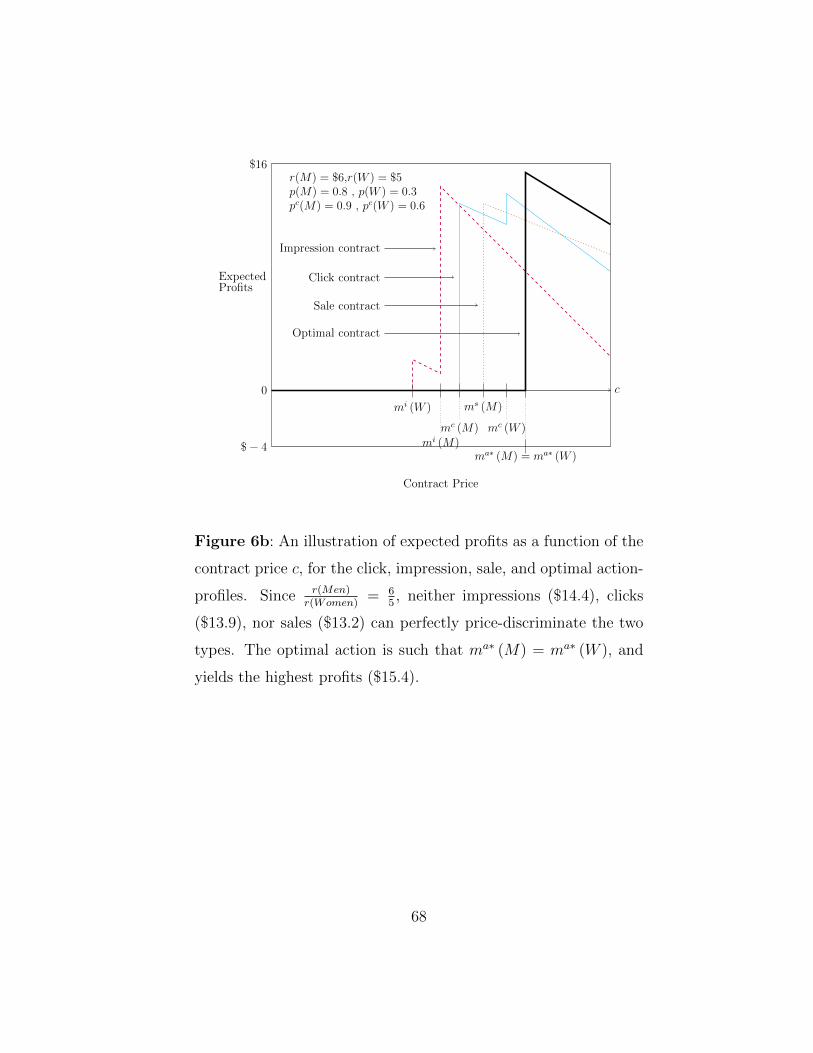
0 c

$16

$− 4

r(M) = $6,r(W ) = $5p(M) = 0.8 , p(W ) = 0.3pc(M) = 0.9 , pc(W ) = 0.6

mi (W )

mi (M)mc (M) mc (W )

ms (M)

ma∗ (M) = ma∗ (W )

Impression contract

Click contract

Sale contract

Optimal contract

ExpectedProfits

Contract Price

Figure 6b: An illustration of expected profits as a function of the

contract price c, for the click, impression, sale, and optimal action-

profiles. Since r(Men)r(Women)

= 65, neither impressions ($14.4), clicks

($13.9), nor sales ($13.2) can perfectly price-discriminate the two

types. The optimal action is such that ma∗ (M) = ma∗ (W ), and

yields the highest profits ($15.4).

68

(a)

0

User Types, t ∈ [0, 1]

p(t)π − r(t)

target with optimal contract

t

ExpectedProfits

(b)

0

User Types, t ∈ [0, 1]

p(t)π − r(t)

∂(ma(t))∂t

Fa(t)

target with increasing ma (t)

ExpectedProfits

Figure 7a-b: Illustration of optimal type-targeting by the pub-

lisher. In (a), by choosing the optimal contract, the advertiser

does not target types for whom marginal benefits do not exceed

69

marginal costs (r (t)). In (b), the choice of any increasing r(t)pa(t)

re-

sults in increasing marginal costs, reducing the set of targeted user

types and overall profits.

70

0 1

$8

ExpectedProfits

F.F. valuation (blue)

Y.C. valuation (red)

epv∗ (t)

F.F. profits

Y.C. profits

Men Women

Figure 8a: Illustration of optimal contract, traffic allocation, and

expected profits under Example A with two advertisers. The fan-

tasy football (F.F.) advertiser has relatively higher valuations for

men than women, while the opposite holds for yoga class (Y.C.) ad-

vertiser. Each advertiser submits a contract which offers per-view

revenue of epv∗ (t) to the publisher, which in this case is the inferior

advertiser’s expected value for each type. The fantasy football ad-

vertiser gains positive profit on men-types, equal to the difference

between the two valuations, while the yoga class advertiser earns

analogous profits for the women-types.

71

0 1

p1 (t) π1

p2 (t) π2

r(t)

traffic captured by Advertiser 1 traffic captured by Advertiser 2

E [ΠAd1 ]

E [ΠAd2 ]

E [ΠP ]

ExpectedProfits

User Types, t ∈ [0, 1]

Figure 8b: Illustration of optimal contract, traffic allocation, and

expected profits under Bertrand price competition with two firms.

Each advertiser chooses a contract price and action-profile such

that earnings-per-view are equal to the minimum between each ad-

vertiser’s expected revenue from type t. This amount becomes r(t),

the reservation price and the expected revenue for the publisher.

Advertiser 1 enjoys positive profits on all t such that expected rev-

enue exceeds that of advertiser 2, while advertiser 2 enjoys similar

positive profits for all other traffic types.

72

Chapter 2

Energy Savings and The Rebound Effect with

Multiple Energy Services and Efficiency

Correlation

Joint with Michael F. Blackhurst1

2.1 Introduction

Energy efficiency has been promoted by a host of policy organizations

as a cost effective means for reducing energy use and respective externalities

NRC [2009], EPA [2008]. Over the last several decades, energy efficiency pro-

grams, standards, and policies have become increasingly common at private

municipalities and all levels of government. There are nearly 1,500 energy

efficiency programs in the U.S., and most programs administer efficiency by

providing financial incentives for technology adoption DSIRE [2013]. Spending

on demand-side management more than doubled between 2005 and 2010 EIA

[2013a], perhaps buoyed by an $11B Federal investment in energy efficiency as

part of the American Recovery and Reinvestment Act of 2009 EIA [2013c].

1Extensive portions of this chapter have been previously published as Ghosh, Neal K.,and Michael F. Blackhurst. “Energy savings and the rebound effect with multiple energyservices and efficiency correlation.” Ecological Economics 105 (2014): 55-66.

73

Supporting arguments for efficiency often assume energy demand re-

ductions are driven exclusively by changing the technical operating efficiency

of durable goods NRC [2009], EPA [2008], Creyts [2007], i.e., an increase

in efficiency leads to an equivalent decrease in energy use (∆Efficiency =

−∆Energy). These approaches are often called “bottom-up” or “engineer-

ing economic” assessments because they apply engineering analysis to assess

individual technologies. Bottom-up assessments often rank-order efficient tech-

nologies by the levelized cost of energy saved, then estimate the technically fea-

sible energy saved assuming all technologies in a given market are replaced or

retrofitted, a format often called a “conservation supply curves.” Recent appli-

cations of bottom-up assessments include NRC [2009], Creyts [2007], Azevedo

[2009], Blackhurst et al. [2011].

However, neoclassical economics indicates consumers respond to effi-

ciency (an implicit decrease in the price of energy services) by increasing

quantity demanded, eroding some of the technically feasible savings (a be-

havior termed the “rebound effect”). The rebound effect for households is

typically divided into direct and indirect effects. The direct rebound effect is

the behavioral change following an efficiency improvement for a single end-

use. The direct effect is defined as the elasticity of a single energy service

with respect to its own efficiency, and is typically derived by differentiating

the definition of technical efficiency (E = S/ε) with respect to efficiency as

per Equation 1:

74

ηε(E) =∂E

∂ε

ε

E=∂(Sε

)

∂ε

εSε

=

[∂S

∂ε

1

ε− S

ε2

]ε2

S=

[∂S

∂ε

ε

S− 1

]= ηε(S)− 1

(2.1)

where E denotes the energy input, while S denotes energy services, and ε

denotes efficiency. The “engineering economic” approach assumes ηε(S) =

0, modeling the elasticity of energy use with respect to efficiency as unity

(e.g. ∆Efficiency = −∆Energy). Equation 1 is conceptually appealing in

demonstrating that some efficiency gains are “taken back” as additional energy

services and has informed much of the literature on the direct rebound effect

Sorrell et al. [2009], Greene [2012]. On the other hand, the indirect effect for

households is typically attributed to re-spending on other goods and services,

largely due to an increase in purchasing power caused by the decrease in the

effective-price of energy (in economics, this is referred to as the “income”

effect). Since energy (and carbon) is used in the supply chain of essentially

any good and service, re-spending will erode the net effects of efficiency. In

combination with broader structural shifts for producers, these re-spending

patterns can lead to “economy-wide” rebound affects Azevedo et al. [2012],

Herring et al. [2009]. On these grounds, researchers and policy makers have

emphasized that rebound challenges the efficacy of efficiency to reduce net

energy consumption Alcott [2010], Jenkins et al. [2011], Barker et al. [2009].

Literature reviews show wide ranges in magnitudes for the direct re-

bound from nearly 0 to 100% Sorrell et al. [2009]; however, considerable vari-

ation in methods, study samples, and research quality may explain these in-

75

consistent results. In particular, previous researchers suggest higher rebound

for lower income households due to higher expected marginal utility for energy

services. By assuming the price of energy is exogenous and efficiency changes

are constant, some researchers assert that the direct rebound, ηε (S), is ap-

proximately negative of the own-price elasticity of demand for energy services:

ηε (S) = −ηp (E) Greene [2012], Sorrell et al. [2009], Binswanger [2001]. These

assumptions serve as the basis for much of the empirical estimates of direct

rebound.

Research on indirect rebound is more sparse. Binswanger [2001] con-

ceptually challenged restricting rebound analyses to a single-service, applying

indifference curves to qualitatively demonstrate that indirect rebound may be

much larger for energy-intensive substitutes and that the income effect may

be much more significant than price responses. More recently, Saunders [2013]

echoed this sentiment. A few studies use Equation 1 to estimate the increase

in expenditures (income and substitution effects) following discrete efficiency

changes Thomas and Azevedo [2013], Freire-Gonzalez [2011]. These studies

using environmentally extended input-output analysis to empirically estimate

indirect rebound as the energy embodied in the production of goods and ser-

vices associated with an increase in expenditures following a discrete efficiency

change. These studies estimate the magnitude of “direct + indirect” effects

ranging from 30%-40% for the U.S. and 30%-50% for Spain.

Several researchers emphasize that technical change can also increase

time efficiency, especially for transportation services. Binswanger discusses

76

two rebound effects for time saving technologies. First, time saving technolo-

gies often require more energy to increase the speed of service, as demonstrated

by faster transportation modes. Second, since time is a constraint similar to

income, time saving technologies produce substitution effects similar to an

income increase. Jalas [2002] emphasized this latter effect in estimating the

potential rebound from a time savings services for Finish households. While

the author acknowledges empirical limitations, results suggest some time sav-

ings interventions – like eating out and using cars for shopping - might produce

a rebound.

The above models of rebound are limited to a discrete efficiency change

for a single service. However, households are subject to ongoing, positively cor-

related efficiency improvements within and across end uses. While exogenous

to households, Federal efficiency standards for a broad array of end-uses have

consistently increased over the last several decades. Endogenous, positively

correlated efficiency change is also observed in above-code technology choices.

The average U.S. household has three above-code efficient technologies in-

stalled; 40% have more than five; 90% have more than two. Figure 1 indicates

that above code technologies installations and consistent above code installa-

tions increase with income EIA [2012]. The energy technology installations

in Figure 1 reflect installations across different energy services that are not

mutually exclusive.

For the purposes of this paper, we call consistent, positively correlated

exogenous and endogenous efficiency change “efficiency correlation.” While the

77

literature demonstrates limited insight into the underlying behaviors driving

endogenous change, there is some intuition behind this occurrence: a house-

hold preferring one above-code efficient technology is likely to prefer others.

Or, in a more dynamic framework, households might use the savings generated

from one upgrade to invest in another (or perhaps compensate by leveraging

efficiency gains in one end use for another). Efficiency correlation challenges

the single service models of rebound dominant in the literature, i.e., models

assuming efficiency changes for only one end-use. Does this marginal change

increase or decrease the rebound effect? Answers to this question involve sev-

eral potential behavioral responses. Some consumer re-spending is associated

with additional efficiency improvements (a reduction in real income), which

then induces a subsequent improvement in technical efficiency (a decrease in

price and increase in real income) and thus additional rebound.

The primary objectives of this paper are to (1) develop a generalized

microeconomic model of the rebound effect that includes distinct but simul-

taneous efficiency changes for two energy services; (2) apply the model to

estimate the potential for rebound across the residential and transportation

sectors; and (3) demonstrate the importance of considering efficiency changes

across multiple energy services when modeling and empirically estimating re-

bound. The scope of our analysis thus includes the direct rebound effect as well

as the indirect effect associated with consumption of a single, second energy

service.

Our model more represents more realistic efficiency change and ob-

78

served technology choices that are more complicated and nuanced than models

assuming discrete efficiency changes for a single-service, such as those reflected

in the direct rebound literature and some indirect rebound models. In par-

ticular, total energy rebound can vary not only with the substitutability of

different energy goods, but also to the degree that efficiency improvement

may occur disproportionately across end-uses and sectors.

2.2 Theory

2.2.1 Motivation

As mentioned previously, one limitation of previous models is the as-

sumption of stand-alone, independent efficiency upgrades in one energy in-

put. However, considerable evidence suggests that many households choose

to make efficiency upgrades across many different inputs, what we call “effi-

ciency correlation.” Under efficiency correlation, the single-service model may

not accurately capture the full response in energy services.

Consider household demand for two energy services (Ei, Ej) with prices

(pi, pj) for a household with income M and energy-efficiency levels (εi, εj).

Generally, demand functions can be written as a function of income, prices,

and energy efficiencies:EiEj

=fi (M, pi, pj, εi, εj)fj (M, pi, pj, εi, εj)

. The full partial derivative

of energy services with respect to efficiency-i is:

(∂Ei∂εi∂Ej∂εi

)=

(∂fi∂εi

+ ∂fi∂εj

∂εj∂εi

+ ∂fiM

∂M∂εi

+ ∂fi∂pi

∂pi∂εi

+ ∂fi∂pj

∂pj∂εi

∂fj∂εi

+∂fj∂εj

∂εj∂εi

+∂fjM

∂M∂εi

+∂fj∂pi

∂pi∂εi

+∂fj∂pj

∂pj∂εi

)

79

The above derivation demonstrates the full partial effect of efficiency

on energy use, taking into account potential endogenous responses to all argu-

ments within the demand function. Given that energy prices are determined

by aggregate supply and demand and not individual efficiency choices, we can

also assume that ∂pi∂εi

=∂pj∂εi

= 0. Moreover, given that the annuitized cost of

efficiency improvements is small and represents a trivial component of income,

we can abstract from income changes and assume ∂M∂εi

= 0. Thus, the full

partial derivative is reduced to:

(∂Ei∂εi∂Ej∂εi

)=

(∂fi∂εi

+ ∂fi∂εj

∂εj∂εi

∂fj∂εi

+∂fj∂εj

∂εj∂εi

)(2.2)

The above derivation demonstrates how the total energy response can

be decomposed into direct effects(∂fi∂εi

), indirect effects

(∂fj∂εi

), and efficiency-

correlation effects([

∂fi∂εj

+∂fj∂εj

]∂εj∂εi

). For the purposes of this paper, we will

characterize three models which represent special and generalized cases of

Equation (2).

• Model I. The engineering-economic approach would predict no change

in energy services due to changes in εi, such that ηεi(Ei) = −1 and

ηεi(Ej) = 0. This can be represented as a special case of (2) where

∂fi∂εi

= −Eiεi

,∂fj∂εi

= 0, and∂εj∂εi

= 0.

• Model II. A neoclassical approach captures direct effects and in some

cases, indirect effects, but considers efficiency changes in isolation. This

is more flexible than Model I, but still a special case of (2) where∂εj∂εi

= 0.

80

• Model III. A model with efficiency correlation, but which only includes

the technical response from a secondary energy service. That is, no

behavioral responses from the secondary efficiency change exist. This is

a special case of (2) where ∂fi∂εj

= −Eiεj

and∂fj∂εj

= −Ejεj

.

• Model IV. A model with efficiency correlation, and the general model

detailed in (2).

Model IV, which we will formally present in the next section, is a more

general model than I, II, and III. We will intermittently refers to the Models

I-IV throughout the paper to compare and contrast the characterizations and

magnitudes of different behavioral responses. Of particular note, is the relative

differences in responses between Models II, III, and IV, since these differences

represent that impact of efficiency correlation.

2.2.2 Model

Our objectives are to consider the impacts of efficiency correlation on

rebound. To do so, it is imperative to develop a model with multiple energy

sources, such that households evaluate not only total energy consumption,

but also the trade-off between each energy source, with plausibly different

efficiencies. Furthermore, given that households do not value energy itself,

rather, consider a factor of production for consumption goods, any appropriate

model must consider some sort of household production.

The model we present here is philosophically rooted in Becker’s house-

81

hold production model Becker [1965], and consistent with similar models ex-

ploited in the literature Binswanger [2001]. Households value consumption,

represented as a composite good Y , and produce consumption using a variety

of inputs. In this regard, the household takes the guise of a firm, and must

weigh the productivity of each input against its price. For our model, we

consider three inputs: electricity work (C), transportation work (T ), and a

composite input representing all other factors (X). Furthermore, we consider

a household production function with constant elasticity of substitution:

Y =[(1− αC − αT )X

σ−1σ + αCC

σ−1σ + αTT

σ−1σ

] σσ−1

(2.3)

α = (αC , αT ) are share parameters for both energy inputs, and σ is

the elasticity of substitution. Generally, the elasticity of substitution between

any two inputs xi and xj is defined as η pipj

(xixj

)=

∂xixj

∂pipj

pipjxixj

, and reflects how, in

percentage terms, the ratio of inputs would change due to a change in the rel-

ative price. Production functions with constant substitution of elasticity were

originally analyzed for the 2-factor case by Solow [1956] and then Arrow et al.

[1961]. Uzawa [1962] showed that when generalized to n factors, the constant

elasticity of substitution property need not be maintained; however, we show

in Proposition 3 that this property is preserved in our model. The constant

elasticity of substitution (CES) production function is a standard modeling as-

sumption in neoclassical microeconomics. Intuitively, this assumption restricts

the household to a constant (again, in percentage terms) trade-off betweens

all inputs. To the extent that agents do not gain direct utility from particular

82

factors of production, this is perhaps a harmless assumption. On the other

hand, there may be lower and upper bounds on certain inputs, for example,

a lower bound on miles driven in each week, which would alter substitution

elasticities, particularly at extremes. Certainly, a CES production function

would be a poor assumption in these scenarios. However, we will continue

with this assumption in concurrence with the literature, and discuss potential

issues in a later sections.

Electricity work is created through electric energy, scaled by electric

energy efficiency, or C = εCEC . Similarly for transportation, T = εTET . The

household has preferences over Y , represented by a concave, twice-continuously

differentiable function, U(·). As will be shown, these properties are all that are

required for our main results to hold. The household faces a budget constraint:

pxX + pCEC + pTET ≤M (2.4)

Without loss of generality, we normalize pX = 1, so that energy prices

are relative, and income M is deflated by the composite input price. The

household’s problem is to maximize utility, U(Y ), with real income M and

relative prices p = (1, pC , pT ). The model is formally defined as follows:

83

V (M, p, εC , εT ) = maxEC ,ET ,X

{U(Y )} : (2.5)

M ≥ X + pCEC + pTET (2.6)

C = εCEC (2.7)

T = εTET (2.8)

Y =[(1− αC − αT )X

σ−1σ + αCC

σ−1σ + αTT

σ−1σ

] σσ−1

(2.9)

0 ≤ (X,EC , ET ) (2.10)

2.2.3 Model Properties and Elasticities

Proposition 1 presents the demand functions for each input, i.e., the

result of the household’s problem described by Equations 5-10. The resulting

demand functions are similar to standard demand functions for CES produc-

tion, with a minor exception. In our model, the household does not choose

energy services directly; rather, they choose energy itself (e.g., that which is

displayed on a utility bill), which becomes a factor of production once scaled

by efficiency. Therefore, the functions are slightly modified from standard

CES functions. Interestingly, the demand functions are independent of U(·),

so long as U(·) is concave and twice-continuously differentiable.

Proposition 2.2.1. If U(·) is concave and twice-continuously differentiable,

then V (M, p, εC , εT ) has a unique solution defined as:

E∗C = MpC

(ZC

1+ZC+ZT

)

E∗T = MpT

ZT1+ZC+ZT

84

X∗ = M(

11+ZC+ZT

), where

ZC =(

αC(1−αC−αT )

)σ (pCεC

)1−σ, and

ZT =(

αT(1−αC−αT )

)σ (pTεT

)1−σ.

Proof. See Appendix.

Before examining the effect of efficiency correlation on rebound, we con-

sider the properties of the CES structural representation proposed in Proposi-

tion1 for simple and extreme cases to build intuition for modeling two energy

services. Proposition 2 shows the own price elasticity of demand for energy

service i. Proposition 2 indicates that the own price elasticity of demand for

energy service is the substitution elasticity that has been adjusted by the bud-

get share. To explain, consider two extreme cases. First, in the single-good

case, the budget share equals one, in which the price elasticity collapses to

one, regardless of σ. This is because with one-service, demand must reduce

one-to-one with a price increase in order to satisfy the budget constraint. On

the other hand, consider a continuous spectrum of services, such that any in-

dividual service has a budget share of zero. In this case, the substitution and

price elasticity are equal. In our analysis, we observe budget shares for energy

inputs which are small but nonzero. Thus, the price elasticities are bounded

between σ and 1.

Proposition 2.2.2. The elasticity of Ei with respect to pi is ηpi(Ei) = (1 −

σ)(1− piEiM

)− 1.

85

Proof. See Appendix.

We can interpret the substitution parameter σ as the “flexibility” home-

owners have in substituting across each energy service. Again, consider some

simple examples. If homeowners have zero flexibility (σ = 0), then relative

price changes do not spur households to substitute away from the relatively

expensive end-use, so households’ optimal mix of energy services remains un-

changed. These are the responses that would be predicted in Model I, and

the price elasticity is simply the budget share, indicating that a price decrease

will lead to a share’s worth of consumption increase for all inputs. If σ = 1,

then households respond completely to relative price changes. A drop in price

results in an exact increase in consumption, leaving nominal consumption un-

changed. If σ > 1, the price elasticity will be much larger than 1, reflecting the

greater “flexibility” homeowners have in substituting across energy services in

maximizing utility.

Proposition 2.2.3. The elasticity of substitution between {EC , X}, {X,ET},

{EC , ET} is constant at σ.

Proof. See Appendix.

2.2.4 Rebound with No Efficiency Correlation

Direct Efficiency Elasticity and Rebound. Proposition 4 shows the elas-

ticity of energy service i, with respect to its own efficiency and the direct

86

rebound effect without any secondary effects of efficiency correlation. Obser-

vation of Proposition 2 shows that ηεi(Ei) = −ηpi(Ei)− 1, which makes sense

given the elasticity of energy with respect to efficiency ought to be compara-

ble to the price elasticity (the ratio piεi

represents the effective price of energy

services). This result also compliments the common practice of using a price

elasticity to approximate rebound for the single-service model.

Proposition 2.2.4. The elasticity of Ei with respect to its own efficiency εi

is ηεi(Ei) =(1− piEi

M

)(σ − 1). The rebound effect is rεi(Ei) = ηεi(Ei) + 1.

Proof. See Appendix.

Cross-Service Efficiency Elasticity and Indirect Rebound. When the

efficiency of Ei increases, not only does this decrease the effective price Ei,

but it also increases the purchasing power (the income effect) over all goods

and services (more colloquially called “re-spending” in some rebound research).

The cross-service elasticity of efficiency, ηεi(Ej), shown in Proposition 5 reflects

this re-spending. Intuitively, the sign of ηεi(Ej) is opposite that of the own

efficiency elasticity (Proposition 4), as reductions of energy service j cannot

be achieved from additional spending on Ej in the case where the technical

efficiency of j does not change. Without technical change in j, ηεi(Ej) is

equivalent to indirect rebound

87

Proposition 2.2.5. The cross-efficiency elasticity of Ej with respect to effi-

ciency i is ηεi(Ej) = −(piEiM

)(σ − 1). Assuming efficiency changes are inde-

pendent, the rebound effect is rεi(Ej) = ηεi(Ej).

Proof. See Appendix.

Total Energy Elasticity. Proposition 6 shows the total rebound effect

(direct plus indirect effects) as the elasticity of net energy use (E = Ei +

Ej) with respect to efficiency change for a single end-use i. Proposition 6.1

indicates that the net energy elasticity is the sum of direct and indirect effects

weighted by their respective energy shares. Similarly, Proposition 6.3 indicates

the “direct + indirect” rebound effect is the direct and indirect effects weighted

by their respective energy service shares. To connect this equation to the

traditional “take-back” perspective, we present Proposition 6.2. Proposition

6.2 shows that the elasticity of total energy use is simply the sum of technically-

driven change (elasticity under technical change alone would equal -1), minus

the portions “taken back” and returned to energy services (direct and indirect

terms), all weighted by their respective shares of energy use.

Proposition 2.2.6. Define the total energy elasticity with respect to efficiency

εi as ηεi(E).

1. ηεi(E) = ηεi(Ei)EiE

+ ηεi(Ej)EjE

.

88

2. Alternatively, it can be written as : ηεi(E) = (−1) EiE

+ rεi(Ei)EiE

+

rεi(Ej)EjE

.

3. The rebound effect is rεi(E) = rεi(Ei)εiEiS

+ rεi(Ej)εjEjS

, where S is total

energy services.

Proof. See Appendix.

2.2.5 Efficiency Correlation

We now consider the generalized conditioned of primary interest: the

influence of efficiency correlation across both energy services i and j. Propo-

sitions 7.1-2 show that the energy elasticity for one service includes both the

direct rebound and secondary, indirect effect associated with efficiency cor-

relation. For Proposition 7.1, efficiency improvements in j follow efficiency

improvements for i (ηεi(εj) > 0). As a result, technical change in j induces

additional spending on energy service i, which is the cross-service efficiency

elasticity, ηεj(Ei). The product of these two, ηεi(εj) · ηεj(Ei), is the indirect

rebound effect of these secondary efficiency changes. Proposition 7.2 follows

similar logic but for energy service j.

Proposition 2.2.7. Define ηεi(εj) as the efficiency-correlation elasticity. If

there is efficiency correlation, then:

1. ηεi,ec(Ei) = ηεi(Ei) + ηεi(εj)ηεj(Ei)

89

2. ηεi,ec(Ej) = ηεi(Ej) + ηεi(εj)ηεj(Ej)

3. ηεi,ec(E) = ηεi(E) + ηεi(εj)ηεj(E)

(a) ηεi,ec(E) =(

(−1)EiE

+ rεi(Ei)EiE

+ rεi(Ej)EjE

)+

ηεi(εj)(

(−1)EjE

+ rεj(Ej)EjE

+ rεj(Ei)EiE

)

(b) ηεi,ec(E) = −1 ·(EiE

+ ηεi(εj)EjE

)+ rεi(Ei)

EiE

+ rεi(Ej)EjE

+

ηεi(εj)(rεj(Ej)

EjE

+ rεj(Ei)EiE

)

4. rεi,ec(Ei) = rεi(Ei) + ηεi(εj)rεj(Ei)

5. rεi,ec(Ej) = rεi(Ej) + ηεi(εj)rεj(Ej)

6. rεi,ec(E) = rεi,cc(Ei)εiEiS

+ rεi,cc(Ej)εjEjS

Proof. See Appendix.

The net energy elasticity under efficiency correlation is the sum of the

standard energy elasticity, ηεi(E), as determined in Proposition 6, plus the in-

duced response from technical change in the second end-use, ηεj(E), weighted

by the magnitude of efficiency-correlation elasticity, ηεi(εj). This is a com-

mon refrain in the derivations that reflect efficiency correlation. Under effi-

ciency correlation, each energy elasticity (and by extension, rebound effect) is

augmented by the subsequent efficiency changes in other end-uses, amplified

by the relative efficiency correlation across services, ηεi(εj). Thus efficiency-

correlation elasticity becomes a critical parameter in determining how much

90

incremental change in energy use is induced. The more disproportionate ef-

ficiency is across end-uses (increasing ηεi(εj)), the more influential these sec-

ondary effects of efficiency correlation become.

Propositions 7.3a-b show the total energy use elasticity in the “take-

back” perspective. Proposition 7.3a groups the full elasticity into the first-

order elasticity from the original efficiency change, plus the second-order elas-

ticity from the endogenous efficiency change multiplied by efficiency-correlation

elasticity. Each “full” elasticity, both first- and second-order, are comprised

of technical, direct, and indirect responses. This proposition looks similar

to 6(b), with the exception that terms associated with correlated-efficiency

changes are included for the technical change, direct rebound, and indirect

rebound. This presentation illustrates how efficiency-correlation can increase

the number of channels through which households can erode energy savings

through behavioral responses. On the other hand, Proposition 7.3b groups the

first- and second-order responses together into technical, direct, and indirect

effect categories. In this grouping, we can see that each category of responses

is augmented by efficiency correlation. Proposition 7.4-6 present analogues

rebound derivations with efficiency correlation.

Table 1 summarizes the derivations above to clarify the connection be-

tween direct rebound as traditionally measured and the total elasticity deriva-

tions, both with and without efficiency-correlation.

We demonstrate our model by considering rebound within and across

residential electricity end-use consumption (denoted by subscript C) and per-

91

sonal transportation by a vehicle using a conventional gasoline-powered inter-

nal combustion engine (denoted by subscript T ). The following sequence of

technical change and respective economic responses summarizes this applica-

tion with an initial improvement in the efficiency of residential electricity end

uses.

1. First-order technical elasticity. This is the engineering-driven change in

energy use, assuming no behavioral response, and equals -1 times the

relative share of electricity.

2. Direct rebound effect. Electricity services is effectively cheaper, resulting

in increased consumption. The increase in energy use is rεC (EC) × ECE

,

or the direct rebound effect multiplied by electricity’s share of overall

energy use.

3. Cheaper electric services results in increased purchasing power, and in-

duces income effects for cross-sector services like transportation. This

first-order “indirect” rebound effect is rεC (ET )× ETE

.

4. Increased energy savings and cheaper energy services lead to higher

real income, and induce the household to upgrade transportation effi-

ciency. Relative to electricity, this percent increase is ηεC (εT ). Thus

total energy use is furthered decreased by the technical change associ-

ated with transportation as a result of efficiency correlation, and is equal

to ηεC (εT )×−1× ETE

.

92

5. Efficiency increases in transportation lead to increase in transportation

consumption due to the effective decrease in price. This increase is equal

to ηεC (εT )× rεT (ET )× ETE

.

6. Cheaper transportation services induce further income effects, and in-

creases consumption of electricity services. This increase is equal to

ηεC (εT )× rεT (EC)× ECE

.

Each effect from 2-3, 5-6 incrementally erodes the first-order (step 1)

and second-order (step 4) technical savings.

2.3 Empirical Analysis and Assumptions

Elasticity of Substitution. We estimate the elasticity of substitution by

observing price elasticities previously estimated in the literature, and back-

ing out σ using Proposition 2 (for both electricity and gasoline). Nationally

averaged consumer expenditures survey data BLS [2011] were used to esti-

mate budget shares for electricity and gasoline at 2.3% and 4.3%, respectively.

Short- and long-run price elasticity data were taken from literature reviews

Dahl [1993], Graham and Glaister [2002], Brons et al. [2008]. Based upon

these data, we assume short- and long-run elasticities of substitution to be

0.15 and 0.9, respectively. Table 2 summarizes these estimates.

Nominal Energy Shares. For the first half of the results section, we

present rebound estimate conditional on income, based on the heterogeneity

in nominal energy shares. Nominal energy shares were calculated by income

93

using the consumer expenditures survey. Households were grouped into $5000

buckets based on annual income. The average nominal share for both gasoline

and electricity consumption were taken, along with the standard deviation

within each group. Finally, both the point-estimates and standard deviations

were smoothed across income buckets using the Hodrick-Prescott filter Hodrick

and Prescott [1997].2Of note, nominal consumption of both gasoline and elec-

tricity decline with income; consistent with Proposition 4 and 5, the rebound

effect will decrease with income as well. We emphasize that these expendi-

tures describe consumption bundles for a range of consumers that may or may

not exhibit efficiency correlation. Consumers that make consistent efficiency

choices, perhaps because of underlying environmental values, may also spend

differently. Several studies suggest mixed results for self-reported behavioral

changes for early adopters of solar photovoltaic panels Schweizer-Reis et al.

[2000], Keirstead [2007], McAndrews [2011]. However, such studies do not

cover efficiency technologies and do not provide consumption information.

Real Energy Shares. To convert nominal energy shares into real energy

shares, we use the price ratio of gasoline and electricity. Historical nationally

and regionally averaged retail prices for electricity and gasoline (in units of

$/delivered energy) are used to estimate these price ratios. Gasoline prices are

2HP (Hodrick-Prescott) filters, while developed and typically used for trend-filtering intime-series data, can be applied to any discrete-interval space with sequential ordering.The HP filter is a nonparametric trend estimator which finds the trend line that minimizessquared deviations away from the observed data, subject to a penalty against changes inthe squared second differences of the trend line. For our analysis, we chose a penalty valueof 50.

94

published nationally, by select states, and by five Petroleum Administration

for Defense Districts or PADDs EIA [2013b]. Electricity sales and revenue data

were organized into regions consistent with those for which gasoline price data

were available EIA [2013c]. Nationally averaged retail price ratios (electricity

to gasoline) for the year 2011 are around 1.2, varying from 1.8 (State of New

York) to 0.8 (State of Washington). With the exception of Washington, all

other regional price ratios were greater than 1. We use 1.2 for our analysis.

Efficiency Correlation Elasticities. We identify end-use efficiency across

various residential electricity and passenger vehicle services based on Federal,

EnergyStar, and best-in-class standards. For electricity services, we include

air conditioning, lighting, refrigeration, water heating, clothes drying, clothes

washing, and dishwashing, which collectively constitute about 60% of residen-

tial electricity consumption and represent nearly all of the residential electricity

end uses historically subject to efficiency standards. The baseline efficiency for

retiring technologies was assumed equal to the Federal efficiency standard as-

sociated with their initial adoption. End-use efficiency changes for individual

services were estimated by assuming three technology swapping scenarios: cur-

rent or near-term minimum Federal efficiency standards (minimum expected

efficiency change), current or near-term EnergyStar standards (voluntarily se-

lected above-code efficiency change), or current best-in-class performance (vol-

untarily selected largest efficiency change). We allow for consumers to switch

technologies by end use (e.g., from CFL lamps to LED lamps) where renova-

tions beyond technology swapping are not required (e.g., from ducted space

95

conditioning to ductless heat pump). These scenarios represent approximately

twenty years of historical efficiency changes over the major electricity end-uses

and conventional gasoline-powered vehicles. Table 3 summarizes the ranges of

efficiency changes defined by the above scenarios.

2.4 Results

Direct Rebound Estimates. To contrast our CES model and empirical

assumptions with other literature, we first consider the direct rebound effect

only as represented in Proposition 4. Figure 1 shows our direct, short-run

rebound estimates with heterogeneity in income, as previous empirical work

has identified income heterogeneity in rebound Milne and Boardman [2000],

Small and Van Dender [2007], Hirst et al. [1985]. Figure 1 shows that the CES

model indicates direct rebound for electricity services and personal transporta-

tion falls with income, as the share of these services is smaller for higher-income

households. This suggests that efficiency upgrades for lower-income households

are likely to lead to more rebound than a corresponding upgrade for higher-

income households. While not the explicit focus of this study, our estimates

of direct rebound compare favorably with literature-recommended empirical

estimates of rebound, which range from 10-30% Sorrell et al. [2009] and 0-50%

Greening et al. [2000]. This result suggests to us that our assumptions about

household utility preferences are plausibly not too restrictive. Moreover, our

model suggests that income heterogeneity and uncertainty and variability in

σ may explain differences in empirical estimates.

96

Total Energy Elasticity. Next, we consider the net energy elasticity

accounting for direct and indirect rebound effects absent positively correlated

efficiency changes, which includes only the terms in Proposition 6. The solid

black line represent the technically feasible elasticity, while the dotted and

dark-grey areas represent the erosion of energy savings due to direct and in-

direct rebound, respectively. Thus, the light-grey area represents the total

energy response. Figure 3 plots total short-run rebound for both gasoline and

electricity showing the contributions from direct and indirect rebound. Im-

portantly, we see that direct rebound comprises an overwhelming contribution

of the total rebound if consistent efficiency changes are excluded. For median

earners (around $45k), the direct rebound for a change in transportation ef-

ficiency is near 18 percent (Figure 1). However, gasoline makes up just 70

percent of the total energy consumption. When both gasoline and electricity

are combined in Proposition 6, the net rebound effect with respect to total

energy use is 14 percent, which is lower than direct rebound estimates because

the response is relative to both energy sources, i.e., is weighted by shares.

Households with relatively large energy shares demonstrate the largest indi-

rect rebound response, which is characteristic of lower income households. This

makes economic sense, as income effects are only meaningful for goods that

nominally comprise a large share of expenditures. Our results suggest that

total rebound, the combination of direct and indirect effects on total energy

services, is around 5-13% for an electricity efficiency improvement, and 10-15%

for transportation efficiency improvement. Also note that total rebound across

97

income is not strictly monotonic as is for direct rebound, as the relative shares

of energy inputs are not monotonic in income.

Efficiency Correlation. We now consider the implications of positively

correlated efficiency changes across energy services on net energy elasticities.

To more fully evaluate the effect of uncertainty and variation in substitution

elasticities (σ), nominal energy shares(piEiM,pjEjM

), and efficiency correlation

(ηεi (εj)), we run a stochastic stimulation of Proposition 7.3, and report the

mean, 5th percentile, and 95th percentile of the results’ distribution. σ was as-

sumed to follow a uniform distribution along the minimum through maximum

literature estimates. Efficiency correlation was computed as the electricity

consumption-weighted average of efficiency choices, which were assumed to be

binomial between Federal minimum and best-in-class options for each service.

Share ranges were drawn from a bivariate normal distribution with means,

variances, and covariance estimated from consumer expenditure data. Fur-

ther simulation details are located in the appendix. It should be emphasized

that these simulation parameters are likely to be correlated by construction

(for example, the efficiency correlation elasticity and nominal energy shares).

However, we have no empirical data to characterize such correlation for these

end uses and treat them as independent.

Figures 4 shows short-run total energy elasticity under Models I-IV.

Because these models are sequentially nested, the differences in magnitude

between bars shown left to right represent the incremental contributions to

the net energy elasticity from each model. The top and bottom panels cor-

98

respond to positively correlated efficiency changes initiated by electricity and

transportation services, respectively.

The broad features of the simulation show that positive efficiency cor-

relation brings about additional energy savings (Model III) which are only

partly offset by additional rebound Model (IV). In both cases, the technical

response from the secondary service alone (Model III) overcomes the energy

increases from conventional rebound (Model II), while the additional second-

order rebound (Model IV) has a relatively minor effect. With electricity as

the primary service, base-case estimates of rebound from efficiency correlation

(13%) are nearly double those of conventional rebound estimates (7%). With

transportation as the primary service, base-case estimates of rebound from

efficiency correlation (16%) are nearly the same as conventional first-order

rebound estimates (15%). These figures suggest that any empirical rebound

estimate which does not control for any simultaneous cross-service efficiency

changes is likely to overstate the rebound effect considerably. Finally, the wide

bands on estimates from Models III and IV speak to the inherent uncertainty

of the efficiency correlation elasticity, suggesting that the total response can

be much larger or just equal to the response without efficiency correlation.

While the lack of precision on these estimates is undesirable, the bottom and

top of the bands represent the absolute highest and lowest elasticity that could

feasibly occur, and so it is reasonable to conclude that the true elasticity lay

within these bounds.

99

2.5 Discussion

Our energy elasticity (rebound) model of two-energy services with dis-

tinct but simultaneous efficiency change indicates that residential rebound

involves more complex consumer-technology interactions than described by

models that assume technical change for only one end use. Efficiency correla-

tion – or consistent efficiency change -across multiple end-uses increases techni-

cally feasible efficiency improvements but also drives additional, second-order

economic responses resulting from income and substitution effects across both

end uses. With respect to rebound, these second-order effects are the indirect

rebound from household energy services with distinct technical efficiencies.

We apply our model to estimate rebound across sectors by considering

rebound between residential electricity end-uses and gasoline use for personal

transportation. We estimate that the technical efficiency across these energy

services has recently been disproportionate (ηεi(εj) 6= 1), driven by differing

relative changes in Federal minimum code and above code standards. Base-

case results indicate that the magnitude of rebound from efficiency correlation

is similar to or greater than other conventional first-order rebound estimates,

even those that include indirect rebound without consistent efficiency change.

Figure 5 shows total energy elasticities given parametric variation in

σ and ηεi(εj) for the median income range ($40-$45k) and mean real and

nominal shares. Figure 5 indicates that efficiency correlation always increases

technically feasible savings over models that assume no consistent efficiency

change (ηεi(εj) = 0), which follows from the observation that neither energy

100

service independently approaches backfire. Disproportionate efficiency change

(ηεi(εj) 6= 1) can significantly affect total energy elasticities, particularly for

small values of σ. If consumers cannot flexibly substitute across energy ser-

vices economically (lower σ), technical change for one service is not readily

“taken back” for a second service. Thus in the short-run (0.1 ≤ σ ≤ 0.2), en-

ergy elasticities (and thus rebound) are more sensitive to disproportionate effi-

ciency change. Short-run responses would be characteristic of energy services

for long-lived durable goods, where multiple efficiency changes are less likely to

occur in the short run (as our model assumes). In the long-run (0.7 ≤ σ ≤ 0.9),

however, consumers eventually do adjust expenditures to changes in prices, in-

come, and technical efficiency. Figure 5 indicates long-run energy elasticities

are much lower (less energy savings or higher rebound), with net energy elas-

ticities less than -0.2 for proportional efficiency change (ηεi(εj) = 1) and slight

deviations from -0.2 for disproportionate efficiency change. Since most em-

pirical studies estimate short-run rebound effects, or extrapolate long-run re-

bound estimates using autoregressive time-series models, rebound effects over

the long-run may be significantly higher than what is typically reported in the

literature.

Our energy elasticity (rebound) model of two-energy services with cor-

related efficiency change indicates that residential rebound involves consider-

ably more endogenous and exogenous consumer-technology interactions than

described by models that assume technical change for only one end use. Com-

plimentary empirical support indicates that these interactions, and in partic-

101

ular correlated efficiency choices, are realistic and that they have a significant

effect on energy efficiency elasticities.

Potential for Backfire. Whether aggregate energy use increases or de-

clines depends critically on to what degree the economic responses, both di-

rect and indirect, may outweigh the technical reduction in energy use. Some

researchers have expressed concern about the relative uncertainty in the mag-

nitude of indirect rebound effects Saunders [2013], Binswanger [2001]. As an

extreme demonstration of potential indirect effects, consider the case of “back-

fire,” which will occur when total energy elasticity is positive. As illustrated in

the appendix, total energy elasticity with respect to energy i will be positive

if either energy input is sufficiently large. In the case where energy i is too

large, an increase in efficiency i can induce such a large income effect that

the increase in energy use j outpaces the absolute decrease in energy i (recall

from Propositions 4 and 5 that direct rebound is declining in Ei while indi-

rect rebound is increasing). On the other hand, for the case where Ej is too

large, both as a portion of the budget and a share of the energy mix, backfire

could occur because the indirect rebound response is magnified to the point

of eclipsing the direct energy elasticity. Consider the case where i = C and

j = T . A potential example would be a homeowner residing in an aggressively

energy efficient home but with a long commute, so that ET � EC . In such

a circumstance, an increase in home efficiency may result in a small absolute

decline in electricity use, while the cross-sector indirect effects may generate

large enough absolute increases in transportation services that total energy

102

use may increase. On the other hand, for a homeowner that walks to work,

the cross-sector economic response would not offset the reduction in electric-

ity, resulting in net energy reductions. Despite these insights derived from our

model, empirical expenditure data indicate the magnitude of rebound is far

from backfire (see Figure 3 for example).

Efficiency correlation presents another channel for backfire. Even with

sufficiently small energy use levels, backfire may occur through a negative elas-

ticity between cross-sector efficiencies (ηεi(εj) < 0). Recall from Proposition 7

that total energy elasticity with efficiency correlation will be positive if:

ηεi(E) + ηεi(εj)ηεj(E) > 0

or:

ηεi(εj) < −ηεi(E)

ηεj(E)

So, if the cross-efficiency elasticity is sufficiently negative, total energy

use may increase as a result of a single-use efficiency increase. The logic is

straightforward: if an increase in efficiency i spurs a decrease in efficiency j,

then total energy use may increase on net. It should be noted that in our

simulations we do not observe such a case because, for all end-uses, even the

minimum-standard efficiency choice still represents an upgrade over the retir-

ing technology. However, we stress that such an outcome is specific to the

current environment, and speaks to the importance of minimum standards.

103

With the exception of the fuel economy standards for passenger vehicles from

1990-2009, Federal code efficiency standards have consistently and routinely

increased. However, reasonable scenarios could invoke negatively correlated

efficiency changes. Some homeowners may compensate when making tech-

nology choices, e.g., justifying the purchasing a fuel inefficient vehicle after

upgrading to an efficient appliance. Homeowners could move to a less effi-

cient home. Mandated technical efficiency standards for one service could be-

come disproportionately more costly, constraining consumers for subsequent

efficiency choices. If these floors did not exist, then theoretically households

could potentially respond to an increase in one efficiency by reducing efficiency

in other energy sectors. While it seems unlikely that a household would choose

to make efficiency changes in opposite directions, it is more plausible to think

that households might respond to exogenously-induced changes (through in-

creases in minimum standards) by decreasing efficiency in other less-regulated

sectors. From a policy perspective, minimum code standards create a “floor”

for these potential efficiency downgrades, and, in turn, the potential for re-

bound from such efficiency combinations.

Qualitatively, our model suggests that exogenous (or federally man-

dated) efficiency minimums across multiple energy services must “keep up”

with each other to avoid this backfire scenario. As an example, suppose home-

efficiency standards increase for a household whose current transportation ef-

ficiency was well above the mandated minimum. If the gains from reducing

transportation efficiency (e.g. swapping out a high-priced, efficient sedan for

104

a cheaper, dirtier SUV) was sufficiently high, or if nominal gasoline consump-

tion was sufficiently low (either through low gasoline prices or low-enough miles

drive), then the household would optimally decrease transportation efficiency

even as home efficiency increases (see end-section of Proofs for details). In

such a scenario, a negative efficiency elasticity would be observed, and total

energy use could potentially increase despite the fact that minimum efficiency

standards weakly improved across all services. This occurrence may partially

explain the spike in adoption of larger, less efficient cars observed from the

mid 1990’s to mid 2000’s, as fuel economy standards were stagnant for vehicles

while Federal standards disproportionately advanced efficiency for electricity

and natural gas end-uses. These arguments suggest that there are diminishing

returns to making more-efficient end-uses “better” if they are being jointly-

consumed with other energy-uses which lag far behind in efficiency.

Finally, we note the empirical limitations of our analysis, particular

concerning the imprecise calibration of efficiency-correlation elasticity. Con-

sumers making an above-code efficiency choice seem likely to make similar

choices across technologies, and Figure 1 suggests this type of consistent tech-

nical change occurs often. (It is likely that some, but few, technology instal-

lations profiled in Figure 1 were not chosen by householders but by builders

or designers.) One of the limitations of our empirical analysis is that we use

expenditure data that may or may not represent consistent adopters of effi-

cient technologies. Such adopters may also use energy technologies in a man-

ner consistent with reducing rebound; thus, expenditures representing typical

105

consumers may be misleading. Unable to control for such unobserved hetero-

geneity, we employ a simplified model of energy use assuming CES preferences,

which may be too restrictive to fully capture nuanced consumer responses to

efficiency improvements. However, empirical data characterizing both tech-

nology choices and observed energy consumption (or expenditures) is elusive,

and as such, we are limited in our modeling approach.

2.6 Conclusions

We develop a microeconomic model of household rebound for two dis-

tinct energy services with distinct but simultaneous efficiency changes. We

then apply the model to consider rebound between the residential and trans-

portation sectors. A range of empirical assumptions indicate that positively

correlated efficiency changes increase net energy elasticities (net energy sav-

ings) but that disproportionate efficiency changes across energy services can

significantly affect net energy elasticities. These effects are driven by second-

order indirect rebound responses induced by consistent efficiency changes across

two energy services. The magnitude of these second-order effects is consistent

with other known sources of rebound. While long-run rebound responses can

significantly erode net energy elasticities, we do not anticipate backfire from

positively correlated efficiency. However, negatively correlated efficiency could

induce backfire, and we discuss the implications of this finding. These results

imply that consistent efficiency improvements across end-uses could keep pace

with and thus temper economic responses.

106

2.7 List of Tables

Table 1: Energy Elasticity Decomposition into Technical and Economic Responses. Note the “-1” term appears in the technicalelasticity column to connect the multiple-service model elasticity terms to the analogous elasticity in the single-service model, as thesingle-service model is very common in the literature.

Model PropositionsT echnical

ElasticityDirect Rebound Indirect Rebound NetEnergyElasticity

1 − Service 2,4 = −1= −ηpi(Ei)

= ηεi(Ei) + 1– ηεi (Ei) = −1 + rεi (Ei)

2 − Service,

Standard5,6 = (−1) · Ei

E = (ηεi(Ei) + 1) · Ei

E

= ηεi(Ej) · Ej

E

= −(

pjEj

M

)(σ − 1) · Ej

E

ηεi(E) = −1 · Ei

E

+ rεi(Ei)Ei

E

+ rεi(Ej)Ej

E

2 − Service,

Eff. Corr.7

= −1 · Ei

E

− ηεi(εj) · Ej

E

= rεi (Ei) · Ei

E

+ ηεi(εj)rεj (Ei) · Ei

E

= rεi(Ej) · Ej

E

+ ηεi(εj)rεj (Ej) · Ej

E

ηεi,cc(E) = −1 · Ei

E

+ rεi(Ei)Ei

E

+ rεi(Ej)Ej

E

− ηεi(εj)Ej

E

+ ηεi(εj)rεj (Ej)Ej

E

+ ηεi(εj)rεj (Ei)Ei

E

1

107

! ! 25!

Table 2: The elasticity of substitution (the change in electricity demands with respect to a change in transportation demands) is estimated using applying budget shares and price elasticities to proposition 2. Reference Good Statistic Horizon Price

Elasticity Budget share

Elasticity of Substitution

Dahl Electricity Median Short-run -0.17 0.023 0.15 Dahl Electricity Lit. recommended Short-run -0.24 0.023 0.22 Dahl Electricity Median Long-run -0.96 0.023 0.95 Dahl Electricity Lit. recommended Long-run -0.8 0.023 0.80 Brons Gasoline Median Short-run -0.16 0.043 0.13 Dahl Gasoline Median Short-/intermediate -0.15 0.043 0.11 Graham Gasoline Lit. recommended Short- run -0.18 0.043 0.14 Brons Gasoline Median Long-run -0.69 0.043 0.68 Graham Gasoline Lit. recommended Long-run -1 0.043 1.0

108

109

Table 4: Incremental Contributions to Net Energy Elasticity with Positively Correlated Efficiency Changes

Model Description Incremental Terms

I First-order technical response −EiE

II Direct rebound for sector i, Cross-sector rebound for sector j (ηεi (Ei) + 1) EiE

+ ηεi (Ej)EjE

III Efficiency-correlation technical response −ηεi (εj)EjE

IV Second-order direct and indirect rebound ηεi (εj)((ηεj (Ej) + 1

) EjE

+ ηεj (Ei)EiE

)

110

2.8 List of Figures

111

! ! 28!

!

Figure 2: Direct rebound estimates for a. electricity and b. transportation using a model of a single energy service with a CES production function. Ranges show one standard deviation in expenditures shares within the indicated income category.

0.0

0.1

0.2

0.3

$7,500 $32,500 $57,500 $82,500 $107,500 $132,500 $157,500 $182,500

AFTER-TAX INCOME CATEGORY!

Series1'

Series2'

Series3'

a. ELECTRICITY

σ = 0.15, ranges show variation in shares

σ = 0.10 (no ranges in shares shown)

σ = 0.20 (no ranges in shares shown)

Ranges commonly

reported for household

services

0.0

0.1

0.2

0.3

0.4

Series1'

Series2'

Series3'

b. TRANSPORTATION

σ = 0.15, ranges show variation in shares

σ = 0.10 (no ranges in shares shown)

σ = 0.20 (no ranges in shares shown)

Ranges commonly reported for personal

transportation

SHO

RT

-RU

N, D

IRE

CT

RE

BO

UN

D

0.0

112

! ! 29!

!

Figure 3: Short-run energy elasticities from a model including two energy services model for an efficiency improvement in either (a) electricity end-uses or (b) transportation. The chart format is cumulative in the y-axis (a “stacked area” chart).

-0.8

-0.6

-0.4

-0.2

0.0 7.5 27.5 47.5 67.5 87.5 107.5 127.5 147.5 167.5 187.5

Annual After-Tax Income ($1,000)

b. energy elasticities following a change in transportation efficiency abset consistent efficiency changes for electricity services

-0.5

-0.4

-0.3

-0.2

-0.1

0.0

Direct rebound Indirect rebound Net energy elasticity Technically feasible energy elasticity

a. energy elasticities following a change in electricity efficiency abset consistent efficiency changes for transportation

Ener

gy E

last

icity

113

114

115

Chapter 3

Negative Equity and Landlock: Welfare

Impacts and Policy Implications

3.1 Introduction

Following a five-year decline in home prices during the Great Recession,

[CoreLogic, 2013b], the incidence of negative equity among homeowners grew

rapidly.1 At the end of 2012, 10.4 million homes, or 21.5%, of all residential

properties with a mortgage were in negative equity [CoreLogic, 2013a], down

from 24% in 2009.2 Previous work has analyzed how negative equity – through

households’ liquidity preferences, nominal loss aversion, or increased transition

costs – may decrease geographic mobility (commonly referred to as “landlock”)

and by extension employment opportunities. In short, negative equity makes

moving more difficult or costly, but not necessarily impossible. For example, a

1A property is in negative equity–also known as being “underwater” or “upside down”–ifthe principal outstanding on its mortgage is higher than the value of the home itself. Thisoccurs when a home loses value, increases its mortgage debt, or a combination of both.

2The principal outstanding on a mortgage, particularly at the beginning of the loan,amortizes very slowly, and thus a significant decline in home prices can quickly wipe awayany incremental gains in home equity. Furthermore, while the typical borrower in nega-tive equity usually initiated their home investment with a high loan-to-value ratio (or lowinitial equity), the magnitude of price declines in some markets like Florida, Nevada, Ari-zona, and California were well above 40% cumulatively, enough to wipe-out equity even inthe conservative government-sponsored enterprises (GSE) mortgages which require a 20%downpayment.

116

homeowner in need of relocation might simply pay off the mortgage with cash

should the need arise; net worth would remain the same, and the homeowner

would be free to go. It would just be a matter of whether such an action were

optimal. What has not been documented in this literature, however, is a key

institutional observation: that underwater homeowners can only complete a

sale if they are able to provide cash to cover their negative equity position.

If non-housing assets cannot offset negative equity (in effect, if a homeowner

is underwater and insolvent), a sale cannot occur. In this case, it is not

that moving is suboptimal, it is in fact infeasible. This will have different

implications for household welfare and policy. So far, the policy response to

the housing crisis has been focused on foreclosure mitigation by way of loan

modifications (interest reductions, changes to amortization, etc.); even so, the

high incidence of negative equity remains. It is not clear that this policy is

optimal; for example, lower interest might make a mortgage more affordable,

but also incentivize the household to stay longer, thereby further decreasing

mobility. Mortgage policy has not yet been finalized in the context of limited

mobility brought upon by negative equity and landlock.

In this paper, I analyze the welfare cost of the landlock effect as repre-

sented by a hard constraint which reduces the spatial choice set for homeown-

ers. To do so, I introduce a job search model with savings where the agent is

restricted from spatially-distant job offers if she is landlocked. This model de-

parts from the literature in that it treats landlock as a reduction in the choice

set, rather than an additional cost to move. The model shows that expected

117

durations (time until a job move occurs) increase as net assets fall, as house-

holds deep-enough in negative equity optimally choose not to search. This

results contrasts with that of a standard model, where households without a

landlock friction would show decreased durations as net assets fall. Further-

more, I find empirical evidence consistent with these results using data from

the Survey of Consumer Finances. Sample data from 2010 show that the rela-

tionship between net assets and expected durations is significantly different for

homeowners who are in negative equity. Importantly, durations fall as assets

fall for households who are above water – consistent with a standard model –

while durations either rise or stay flat for underwater households.

Additionally, I leverage the model to analyze the welfare impacts of

comparative mortgage-finance policies. I simulate the model under two policy

adjustments, i) reducing the cost of debt, and ii) lifting the landlock con-

straint, and consider the differential effects on labor supply, expected dura-

tions, and welfare. My results show that reducing the cost of debt, while

welfare-increasing, has no meaningful effect on labor supply or mobility. In

fact, homeowners who are currently landlocked remain so, even choosing to

save less than before. In my model, debt subsidies represent little more than a

wealth transfer between the household and the mortgage holder. Meanwhile,

removing the landlock restriction results in lower durations and higher welfare.

Households are better off being able to search and obtain better employment

opportunities when they are underwater, rather than receiving interest reduc-

tions. In fact, I estimate that median earners would be willing to pay between

118

3-4 percentage points of additional interest on their debt to lift this restriction.

This result suggests that the landlock effect represents an incomplete lending

market. If feasible, homeowners would be willing to compensate lenders to

swap-out mortgage debt with other loans which do not constrain mobility.

This paper will proceed as follows. Section 2 will background on nega-

tive equity, landlock, relocations, mortgage finance policy, and related litera-

ture. Section 3 will introduce the job search model and calibration. Section 4

will describe the SCF data, provide graphical evidence in support of landlock,

and present regression results. Section 5 will present welfare estimates from

competing policy scenarios. Section 6 concludes.

3.2 Background

3.2.1 Relocation and Landlock

It has long been argued that negative equity affects homeowners’ ability

to move. Selling a home that is underwater requires providing additional liquid

assets to make up the difference between the home value and the remaining

mortgage principal. Previous work has focused on discovering whether this ad-

ditional cost hampers mobility, a debate which has not yet reached agreement.

However, what appears to be missing from this discourse is the nontrivial con-

cern that without sufficient assets to offset the negative equity accrued in the

home, the homeowner’s ability to sell becomes functionally obsolete. These

homeowners are referred to as “landlocked,” and are geographically immobile

not by choice (e.g. to avoid the additional costs of moving), but because they

119

are legally and financially restricted from selling. Not typically addressed in

the literature, this is an important distinction, as it renders alternative spatial

and employment choices as infeasible, not just suboptimal.

A simple example might illuminate the distinction. Suppose there are

two homeowners, A and B, who both have a negative equity position of $10,000.

That is, both homes are worth $10,000 less than the corresponding principal

on their mortgages. Homeowner A has non-housing assets of $20,000, while

homeowner B has $0. Therefore, the former is financially solvent, while the

latter is not. Now, let’s say both homeowners were evaluating a decision to

move. To sell her home, homeowner A would have to pay the mortgage holder

$10,000. This is an additional cost to move, and depending on her preferences,

may or may not be a cost she is willing to pay. For example, she may have

a desire to keep $20,000 in liquid assets as opposed to $10,000, which is all

she would have left after the sale. This is how negative equity frictions are

typically incorporated in the literature. Agents have varying wealth positions

in their homes, and negative equity results in higher moving costs which can

reduce mobility and/or increase aggregate unemployment over geographical

regions. However, homeowner B, with the same negative equity position, is in

a completely different situation. Because he has no other assets, there is no

way he can pay the mortgage holder if he were to sell. Regardless of whether

he might choose to pay this cost or not, he is financially restricted from even

considering the option. This example illustrates that one’s negative equity

position alone does not create true landlock; rather, it is the combination

120

of negative equity and net assets which determines whether a conceivable

move is feasible or not. For homeowner A, moving is feasible but costly. For

homeowner B, moving is impossible.

Recent estimates suggest that about 8-10% of households per year ex-

perience a permanent relocation[Ferreira et al., 2010, Molloy et al., 2011]. In

addition, since about 2001, just under 20% of new hires involved the employee

relocating for the position [Cha, 2010].3 As such, a nontrivial fraction of the

population faces a joint moving-employment problem each year, and this prob-

lem has become significantly more complex in the wake of large house price

declines which have eroded household wealth. According to Survey of Con-

sumer Finances, home equity represents a large share of their total wealth for

many homeowners, and a borrower in negative equity is also increasingly likely

to be balance-sheet insolvent.4 Relating back to the previous example, an av-

erage homeowner is more like to look like homeowner B than homeowner A.

Balance-sheet insolvency, unlike cash-flow insolvency, does not immediately

lead to default.5 This is because negative equity is not realized in a cash-

on-hand sense, only in the market value of the home and its corresponding

mortgage. Thus, a homeowner with negative equity is under no legal or finan-

cial sanction as long as they generate enough cash flow to make their monthly

3More recently, this figure has fallen significantly, mainly due to the prevalence of workingvia remote-desktop-connection [Cha, 2010].

4As mortgage-financing conditions have become more accommodating over time, theshare of homeowners who use their home as their primary wealth-building vehicle has in-creased .

5In fact, the majority of homeowners in negative equity continue to meet their mortgagepayments on time [CoreLogic, 2013c].

121

mortgage payments.

Economic theory might suggest that it would be better for these home-

owners to “walk away” from the property, to strategically default on the mort-

gage and wipe away their negative equity position. There is some evidence to

support this: a recent study by oli [2010] concluded that about 20% of serious

delinquencies in 2008 were strategic, while Guiso et al. [2009] put this figure

close to 26%. However, there are several costs associated with default. These

include tangible costs like a damaged credit score as well as intangible costs

like shame and guilt caused by deviating from the perceived social norm of

honoring financial obligations [White, 2010]. Also, as long as the homeowner

has enough cash to make monthly payments, while also expecting the home

value to eventually exceed the mortgage principal at some future date, then it

would be perfectly rational not to default. For example, a Fed study found that

homeowners do not begin to strategically default until after the mortgage ex-

ceeds the home value by about 62%, a relatively high threshold where it would

seem very unlikely that the homeowner would regain positive equity within a

reasonable timeframe [Bhutta et al., 2010]. Also, a separate Boston Fed study

of a house-price decline in Massachusetts in the early 1990s found that less

than 10% of homeowners in negative equity eventually defaulted. Moreover,

there may be additional complications to the default decision based on the de-

cision to file bankruptcy as well [Foote et al., 2008]. While the incidence and

motivating factors behind strategic defaults is an important research topic, it

will not be the focus of this paper.

122

Rather than defaulting, the primary downside of balance-sheet insol-

vency is the “landlock” effect, the inability to transact on the home in a

financially-material way.6 To reiterate, this is a hard constraint, not merely

an additional cost to the homeowner. Because the home is collateral for the

mortgage, the home cannot be sold without making the mortgagor “whole,”

or paying off the full principal of the mortgage.7 If a landlocked homeowner

cannot move, it follows that the homeowner would be unable to accept employ-

ment opportunities that lay outside her current residential area. Both firms

and workers are worse off by this inability to match. In particular, workers

who have the ability to earn higher wages in other locations are unable to do

so, and so their welfare is reduced by being restricted to choose their current

residential location. Furthermore, previous research suggests that labor mobil-

ity, rather than job creation and destruction, is the main adjust mechanism in

labor markets [Blanchard et al., 1992]. Such findings make it clear why land-

locked workers could decrease employment on a national scale; for example,

a recent IMF study suggests that the housing crisis has increased skills mis-

matches at the county level and contributed 134% to structural unemployment

nationwide [Estevao and Tsounta, 2011].

6This can include applying for auxiliary credit, making long-term investments with largeupfront costs, and mostly importantly, selling.

7A homeowner can complete a “short sale,” but this requires the agreement of the mort-gage holder to effectively lower the notional amount of the debt, and is significantly moredifficult to consummate.

123

3.2.2 Policy

The policy response to the housing crisis has been swift and aggressive,

but almost exclusively focuses on mortgage payment reduction. An extensive

review is provided in the appendix, while a brief summary is provided here.

At the onset of the financial crisis in 2007, the main policy goal was to stabi-

lize the mortgage-backed securities (MBS) market. For example, the Federal

Reserve was quick to accept MBS as collateral for loans from the discount

window and through the Term Auction Facility [Bernanke, 2009]. Later on,

the purchases of new MBS became a staple of each quantitative easing mea-

sure put forth. It was not until February of 2009 that the federal government

unveiled a policy specifically designed for current borrowers, the Homeowners

Affordability and Stability Plan. This policy consisted of two programs, the

Home Affordable Modification Program (HAMP), and the Home Affordable

Refinance Program (HARP). The HAMP was designed to encourage lenders,

through various guidelines and subsidies, to modify mortgages for an estimated

7 to 8 million struggling homeowners. These modifications included reducing

interest, extending amortization schedules, and in some cases writing-down

principle, all in the hopes of lowering the probability of borrower default and

increasing the present expected value of the mortgage . The HARP, on the

other hand, was a financing vehicle designed to help homeowners with high

loan-to-value ratios refinance on more favorable terms.8

8Both of these programs were administered by the Federal Housing Finance Agency.

124

While both measures helped to alleviate the threat of cash-flow insol-

vency, neither provided much assistance towards reducing balance-sheet insol-

vency. There are a few problems associated with this general approach. First,

as detailed by Mulligan, requiring that mortgage modifications be indexed to

income inadvertently transforms these measures into means-tested programs.

Thus, adhering to the qualifying prerequisites institutes an implicit income tax

of 31% for borrowers applying for modification [Mulligan, 2009, 2010]. Fur-

thermore, even with a strong policy push towards modification, a 2009 Boston

Fed study found that only 3% of all delinquent mortgages have been modified

[Adelino et al., 2013]. With the exception of the rare principal write-down

in the modification process, none of the policies mentioned above specifically

target negative equity homeowners. If negative equity restrains mobility and

hampers employment, then eliminating the landlock effect imposed by negative

equity could yield substantial benefits in the labor market by “unlocking” la-

borers who were previously geographically immobile. To my knowledge, there

has been little discussion in the literature on optimal mortgage-finance policies

to combat negative equity.9 If these effects are significant, policy may need to

9An exception would be Posner and Zingales [2009], who advocate for a policy which al-lows underwater homeowners to force a renegotiation of the principal down to current value,in exchange for a shared equity agreement on the future appreciate of the home betweenthe homeowner and lender. This plan specifically targets the negative equity problem, andalthough the authors focus on the negative costs associated with foreclosure, would indi-rectly remove the landlock constraint as well. What remains unclear, however, is whetherthis plan would pay off for lenders. For example, my model predicts that durations aredramatically reduced once the landlock friction is lifted. If the homeowner was quick tosell upon the restructuring, it seems unlikely that the lender would break even through aequity stake in the future appreciation of the home. Also, as previously mentioned, theincreasing complex ownership structure of mortgage debt makes the feasibility of such an

125

be modified or expanded to address them.

3.2.3 Related Literature

This paper relates to several different portions of the extensive litera-

ture on relationships between home-ownership, equity, mobility, and employ-

ment. First, there is a broad literature which studies the effects of homeowner-

ship on employment, beginning with the Oswald hypothesis that homeowners

suffer longer unemployment durations (a non-exhaustive list includes Oswald

[1996], Coulson and Fisher [2009], Munch et al. [2006, 2008], Taskin and Ya-

man [2013]). Within that is a growing empirical literature on the the effect

of home-equity on mobility. Using individual-level mortgage data from a New

England commercial bank, Chan [2001] estimates a proportional hazard model

of residential durations, and finds that higher loan-to-value (LTV) ratios de-

crease mobility, with the partial effect amplifying as the LTV ratio increases.

Ferreira et al. [2010, 2011] use the American Housing Survey to find that the

occurrence of negative equity reduces the probability of moving by 30%, while

Schulhofer-Wohl [2011] finds no meaningful effect using the same data. Mean-

while, Donovan and Schnure [2011] look at county-level statistics from the

American Community Survey, and find that negative equity primarily reduces

within-county mobility, but either has no effect or sometimes even increases

out-of-county mobility. It remains the case that the literature has not agreed

agreement questionable. Still, the plan points in the right direction as combating negativeequity, rather than mortgage payments, as the main source of mortgage-finance troubles inthe current climate.

126

upon the sign of the housing-mobility or negative-equity-mobility relationship.

There are competing hypotheses which could explain both results. On the one

hand, negative equity can create landlock, or simply add to the cost of moving

for a homeowner. On the other, negative equity could proxy for poor economic

conditions, in which owners and renters alike choose to migrate for better op-

portunities. I provide some empirical evidence from the Survey of Consumer

Finances which is consistent with the former argument, thought it should be

stated that the dataset and analysis is limited in its ability to differentiate

these two competing hypotheses.

This paper also relates to a macro-based literature which studies how

negative equity affect regional movements and unemployment. Estevao and

Tsounta [2011] construct a skills-mismatch index for each state and find that

structural unemployment has been affected by both skills-mismatches and poor

housing conditions to the tune of 134

percentage points since the onset of the

Great Recession. On the other hand, Valletta [2013] shows that house-lock

has no meaningful effect on unemployment durations. Meanwhile, theoreti-

cal models with heterogenous geographic sectors and residential statuses have

consistently found that falling home prices can lead to reduced mobility and

aggregate unemployment. Some authors attribute this to the difficulty of af-

fording a new downpayment when prices decline [Karahan and Rhee, 2013,

Sterk, 2010], while others look to the liquidity impacts from selling [Head

and Lloyd-Ellis, 2012, Hollenbeck, 2010]. Nenov [2012] describes an economy

where debt overhang creates a default penalty which distorts migration deci-

127

sions. These papers all seek to explain recent macroeconomic events by incor-

porating housing and negative equity frictions, but do not focus on the welfare

costs of those frictions, nor on the optimal policies to address them. Finally,

this paper builds off the joint-asset and search problem as detailed by Chetty

[2008]and Lentz and Tranaes [2005]. However, both consider these problems

in the context of unemployment insurance, while I focus on mortgage-finance

policy.

This paper makes three contributions to the literature. First, I con-

sider the landlock effect as a reduction in the spatial choice set, rather than

an increase in cost. This innovation more accurately describes the imposition

of negative equity when the homeowner has no offsetting assets to finance a

sale. As such, policy can be evaluated not just through varying net assets,

but through eliminating the landlock constraint directly. Second, I estimate

the welfare cost of this restriction in the context of a search-theoretic model

where agents are restricted from accepting spatially-distant job offers. Such an

estimate is useful for analyzing mortgage-finance policy, and has not been ex-

tensively addressed in the literature. Finally, I consider alternative mortgage-

finance policies and their effects on landlock, durations, and welfare. I show

that the current policy of loan modification and reducing the service cost of

debt has no materially effect on durations, and could be improved upon with

policies specifically geared towards reducing the incidence of landlock.

128

3.3 Search Model

In this section, I introduce a general search model with saving/borrowing,

then introduces the landlock effect. Then, I describe and calibrate an explicit

model for simulation which follows closely to Chetty [2008]. Finally, I present

baseline model results.

3.3.1 Model

3.3.1.1 Standard Search Model

Consider a representative agent with current income stream w and cur-

rent net-assets A. One can think of A ≥ 0 representing balance-sheet solvency

and A < 0 representing balance-sheet insolvency. The vector (A,w) thus char-

acterizes the state of the agent. The agent lives in a home which she owns and

thus A represents the net-of-principal outstanding value of their home, plus

other non-housing, liquidable assets. Agents can earn a (1 + r) gross interest

rate on their assets, and discount future consumption streams by a rate of

β = 1/(1 + r). Furthermore, w can represent current wages if employed, or

some other benefit level if unemployed.

The agent is offered another employment opportunity each period, char-

acterized by its level of income w′. For simplicity, assume that once the agent

switches she keeps that job permanently. The offered wages are drawn from

a distribution that is conditional on search effort, F (w′|s). While keeping the

functional form of F (w′|s) general, the basic properties are that F (w′|0) = δ0,

meaning that no search effort yields a wage offer of zero with certainty, and

129

that EF (w′|s)[w′] is increasing in s, implying that the marginal benefit of search-

ing is positive. The cost of searching is represented by an increasing, strictly

convex function, c(s), with c(0) = 0. Once the agent receives her offer, she

can decide to either keep her current income stream, or accept the new offer.

The timing of the agent’s problem is:

1. First, the agent chooses net-asset levels for tomorrow, A′.

2. The agent chooses s, and a wage offer is drawn based on conditional

distribution F (w′|s).

3. If applicable, the agent chooses to accept or reject the wage offer.

Let the agent’s utility be an increasing, strictly concave u(c). Then, the agent’s

problem can be represented as the following Bellman equations:

V (A,w) = maxA′≥−A

{u ((1 + r) · A− A′ + w) +

maxs≥0

{βEF (w′|s) [max (V (A′, w), J(A′, w′))]− c(s)

}} (3.1)

J(A,w′) = maxA′≥−A

{u ((1 + r) · A− A′ + w′) + βJ(A′, w′)}} (3.2)

The additional constraint A′ ≥ −A is a lower-bound for savings, which

is common in infinite horizon models with borrowing. Without a lower bound,

it is plausible that an agent can choose to borrow without limit, servicing exist-

ing interest by accumulating additional debt, in a Ponzi-scheme type fashion.

130

In my simulations, I consider A = 50, 000, which for reasonable interest rate

levels is never binding.

3.3.1.2 Search Model with Landlock

To incorporate the landlock friction, I construct the indicator variable

1(A′ ≥ 0), which equals 1 when the agent has (post-savings) enough assets to

sell and relocate, and equals 0 when she does not. This variable mechanically

renders the value of holding the better-paying job worthless when the agent is

in negative equity. The Bellman equations become:

V (A,w) = maxA′≥−A

{u ((1 + r) · A− A′ + w) +

maxs≥0

{βEF (w′|s) [max (V (A′, w′),1(A′ ≥ 0) · J(A′, w′))]− c(s)}

}(3.3)

J(A,w′) = maxA′≥−A

{u ((1 + r) · A− A′ + w′) + βJ(A′, w′)}} (3.4)

While the indicator variable is a crude instrument for such an exposi-

tion, it captures the main feature that when a household is landlocked, jobs

which require relocation are out of reach, and thus removed as a choice vari-

able. This is a key distinction from the common hypothesis that negative

equity simply increases moving costs to the household.

To summarize, agents choose A∗, which by extension characterizes

131

search effort s∗(A∗). Finally, a key metric of interest is that of expected dura-

tion, defined as:

E(D) =∞∑

t=1

ts∗ (A∗t )t∏

j=1

(1− s∗ (A∗t )) (3.5)

Expected duration captures not only the current probability of find a

job, but the dynamic impacts of future asset choices and their effects on future

probabilities as well.

There are some key limitations of this model. First, the model unnec-

essarily restricts offers within the agent’s location; in reality, workers search

for and receive wage offers that do not require moving. Thus, this model can

be thought of as representing laborers who do not receive better offers within

their location, or have already claimed the highest local wage offer possible.

Second, in real life homeowners amortize part of their mortgage each month

as they make their mortgage payments; this suggests that over time a home-

owner can resolve their negative equity without relying on home price gains

or additional savings. A more accurate model might include a law of motion

for housing wealth which would include this effect. I chose to omit this fea-

ture because resolving negative equity solely through loan amortization is a

lengthy process, particularly at the beginning of the mortgage, and thus on

a per-period basis would not make much of a difference. Third, the assump-

tion that the household keeps the better-wage offer indefinitely restricts the

household from future on-the-job search, which admittedly abstracts a fair bit

132

from reality, and does not adequately characterize separations or transitions.

However, this is the same assumption as in Chetty [2008] as well as Lentz and

Tranaes [2005], both of which focus on the joint savings and search decision. If

future on-the-job search added more value to a current wage opportunity, then

this would more so affect the wage-search relationship rather than the asset-

search relationship and the analysis of alternative mortgage-finance policies,

which is of focus here. Finally, by modeling housing and non-housing assets

jointly, I incorrectly restrict an agent with positive home equity but negative

assets elsewhere. In reality, a household’s non-housing debt does not preclude

them from relocating, so long as they have positive home equity. However,

the fact that one’s residence is the primary asset accumulation vehicle for

most homeowners implies that this occurrence is unlikely. In addition, since

mortgage financing in the U.S. is subsidized relative to other forms of debt, a

homeowner in such a situation would optimally choose to borrow against the

home to pay off that debt. In sum, the model omits some key features of the

housing, mortgage, labor, and lending markets, but these omissions are not

instrumental to the key results I want to derive, and ultimately would create

more complexity than improvement.

3.3.2 Explicit Model for Simulation and Calibration

For simulation, I follow a similar framework as proposed by Chetty

[2008]. Consider an agent who can only obtain a single wage offer equal to

w′ = (1 + ρ)w, where ρ > 0, and will take the offer if received. Intuitively, the

133

value of ρ represents the standard raise an agent receives when she finds better

employment. Since the distribution of wage offers is a singleton, there is no

reservation-wage choice. Moreover, consider search effort s to be normalized to

equal the probability of finding that job in the current period. With probability

s, the agent receives wage offer w′ = (1 + ρ)w, and with probability (1 − s),

she receives no wage offer, or w = 0. Hence, we see that in the standard search

model:

EF (w′|s] [max (V (A′, w), J(A′, w′))] = (1−s)V (A′, w)+s·J(A′, (1+ρ)w), (3.6)

which is consistent with the properties of the wage distribution in the

general model described in Section 3.1. Similarly, for the model with the

negative equity friction:

EF (w′|s] [max (V (A′, w), J(A′, w′))] = (1−s)V (A′, w)+s·1(A′ ≥ 0)·J(A′, (1+ρ)w).

(3.7)

With frictions, the agent can begin receiving the new income stream if and

only if her net asset level A′ ≥ 0. The agent’s problem can be written as:

V (A,w) = maxA′≥−A{u ((1 + r) · A− A′ + w) +

maxs∈[0,1]

{β [(1− s)V (A′, w) + s · 1(A′ ≥ 0) · J(A′, (1 + ρ)w)]− c(s)}} (3.8)

134

J(A,w) = maxA′ {u ((1 + r) · A− A′ + w) + βJ(A′, w)}} (3.9)

The model above is identical to the Chetty model with some distinc-

tions. First, I consider an annual time period instead of weekly. Hence, I

include a nonzero discount rate. Secondly, I include the term friction variable

1(A′ ≥ 0) which renders the value of holding the better-paying job worthless

when the agent is in negative equity.

In line with Chetty’s model, I consider the constant relative risk aver-

sion (CRRA) utility function: u(c) = c1−γ

1−γ . Note that u(c) > 0, ∀c > 0,

implying that V (A,w) > 0 and J(A,w) > 0 for all relevant values of A and

w. Next, I consider the search-cost function c(s) = θ s1+κ

1+κ. With θ, κ > 0, this

function satisfies the properties of the general cost function in Section 3.1.

3.3.2.1 Parameter Assumptions and Calibration

Aside from A, which is predetermined at $50,000, the model has five

parameters Θ = (γ, θ, κ, r, ρ). To calibrate the model, I rely on the data

from the Survey of Consumer Finances. The survey asks households how

long they expect to remain in their current employment state, whether fully-

, partially-, or unemployed. Next, I choose five asset levels (in thousands)

L = {−50,−25, 0, 25, 50}} and compute local conditional averages for wages,

w (i) and expected durations, D (i). Finally, I use an indirect inference tech-

nique that minimizes the squared deviations between the model-generated and

135

sample durations for all five asset levels. Formally, the parameters are esti-

mated as followed:

Θ = argminΘ

{∑

i∈L

(E [D (i, w (i) ,Θ)]−D (i)

)2

}(3.10)

In essence, this procedure calibrates the model by matching the shape

of the model’s duration-assets curve to the sample data for asset levels from -50

to 50 thousand. The results are tabulated in Table 1. The coefficient of relative

risk aversion is well within ranges estimated by Chetty [2006]. Meanwhile, the

estimated nominal interest rate of 5.4% is right in line with typical discount

rates, and the estimated wage premium near 19% is within range of industry

estimates . In both comparisons to the data and to estimates from previous

work, the parameter values appear reasonable.

3.3.3 Baseline Model

Figures 1-3 plot optimal search effort, savings, and expected duration,

with net assets on the horizontal axis, and four relevant income levels high-

lighted. These are the average annual level of unemployment benefits in the

U.S. ($15,000), as well as the first three quartiles of the U.S. income distribu-

tion ($25,000, $45,000, $90,000) . To numerically solve the model, I discretize

the net asset space into $1000 increments.10

10To ensure that the nonnegativity constraint c ≥ 0 never binds, I restrict w ≥ 5000 andA = 50000.

136

The model makes clear that agents in deep enough negative equity

chooses to eliminate search effort, although this threshold varies with income.

Search effort increases abruptly at an asset-level (conditional on income) where

the agent aggressively saves, and chooses assets equal to zero. Then, search

effort gradually reduces as assets increase above zero, as the marginal utility

of income declines. Interestingly, this latter result was the key insight from

Chetty’s work on optimal unemployment insurance that search effort is de-

clining in net assets, and thus, benefits are more valuable for agents with low

assets. However, in a model with negative equity frictions, this monotonic re-

lationship no longer survives. An agent with low-enough assets will eliminate

searching if there is no financially viable way to sell an underwater home in

order to relocate.

We can see in Figure 2 that agents of all incomes choose to save, often

aggressively so, to reduce their negative debt positions, and eventually lift the

landlock constraint. In fact, for small enough debt positions, agents save in

lump-sum to clear the landlock threshold. As the agents’ net asset position

approaches zero from below, the agent reaches an implicit “reservation” net

asset level for each income level, A(w). For initial assets A < A(w), A′∗ < 0,

and s∗(A′∗) = 0. However, for A ≥ A(w), the agent optimally chooses A′∗ = 0

to remove the negative equity friction, and thus s∗(A′∗) > 0. This property

is consistent with Adelino et al. [2013] that many homeowners self-cure their

financial woes. It is also consistent with the recent pattern of aggregate mort-

gage credit among U.S. households. From the household obligations data from

137

FRB, in the 5 years before the Great Recession, mortgage credit increased on

average 1.0% per quarter; in the five years after, mortgage credit decreased

1.2% per quarter . Combined with anecdotal evidence, it suggests that home-

owners are aggressively reducing their debt positions. As the model shows, this

behavior is engendered because agents in negative equity cannot seek better

wage offers, and despite the current-period utility loss of decreased consump-

tion, agents find it optimal to aggressively save to attain better wages in the

future.

Figure 3 plots expected duration for each income level. Durations are

increased for very high and very low assets, but for very different reasons. The

former occurs because agents choose to search less because of the diminishing

return of additional income. Agents with low-enough assets choose not to

search because they are landlocked and cannot accept a new position even if

offered.

3.4 Empirical Motivation from the Survey of ConsumerFinances

To motivate the search-theoretic model with landlock constraints, the

following section provides some further empirical evidence of landlock effects,

in addition to the related literature above. Specifically, I utilize the Survey of

Consumer Finances to test whether the incidence of landlock, separate from

just negative equity or net-worth positions, increases expected employment

durations. The Survey of Consumer Finances provides detail on households’

138

expected duration in their current residences and occupational statuses, as well

detailed financial information on net assets and home equity. Combined, they

provide a glimpse of how durations might change between land-locked and

freely-mobile households. Section 4.1 offers a data description and graphical

evidence, while Section 4.2 presents the regression model and output. Section

4.3 concludes.

3.4.1 Data Description and Graphical Evidence

The Survey of Consumer Finances (SCF) is a questionnaire conducted

by the Federal Reserve Board every three years on the demographic, financial,

and occupational characteristics of U.S. households. The main goals of the sur-

vey are to capture aggregate patterns in household saving, investment, wealth

accumulation, income prospects, and expectations. I use the SCF from 2010

since, because of its concurrence with the decline in home prices, contains

the sharpest variation in the incidence of negative equity. The 2010 survey

includes responses from 6,482 families, totaling about 5300 variables. The pri-

mary attraction of the SCF data is the in-depth detail of asset holdings and

net worth. An ideal dataset to test the landlock constraint would be one which

contained home equity levels, net asset levels, and search-related characteris-

tics like effort and durations. While to my knowledge this ideal dataset does

not exist, there were several alternatives which captured some features which

were needed for this exercise. For example, the Health and Retirement Survey

(HRS) collects asset and debt holdings data along with expectations of future

139

employment. However, the data on home equity itself is quite sparse and im-

precisely surveyed. Additionally, the sample of soon-to-be retirees is not likely

to be representative of the full population. Also, Krueger and Mueller [2010]

leveraged data from the American Time Use Survey (ATUS) to identify search

effort patterns among unemployed laborers. However, it does not appear that

the ATUS publishes information on survey respondents’ asset portfolio, mak-

ing identification of negative equity effects infeasible. Finally, the Survey of

Income and Program Participation (SIPP) is rich in the details of employment

prospects, durations, and moves, but unfortunately it lacks the necessary de-

tails in real estate holdings to impute home equity.11 Therefore, the SCF’s

combination of rich (and complete) net worth details along with viable proxies

for job-search activity and expectations made it the best data option among

the alternatives.

Table 2 presents summary statistics of the SCF data, split between

positive and negative equity households. First, the SCF relatively under-

samples negative equity households (5% in the SCF compared to about 25%

according to CoreLogic). There are an additional 8% of households who are

insolvent but not underwater. Also, homeowners in negative equity are on

average younger, more likely to be in the labor force, have more kids, have

slightly more income, have less wealth, and about 4 times more likely to be

financially insolvent. Note that the survey is over-sampled in high-income,

11The SIPP asks respondents if they hold a mortgage, but do not collect data on homeand mortgage values.

140

high-wealth households which pushes up average statistics relative to the U.S.

population; for the remainder of the analysis, I will restrict the sample to those

individuals whose absolute value of net worth is below $1,000,000.

While the SCF does not collect data on specific job search activity, it

asks other questions which are plausibly affected by the respondent’s job search

effort, mobility, and their expectations of future employment developments. In

particular:

• Section R, Work and Pensions: (If full-time employed) How many years

do you expect to continue working for this employer? (If part-time em-

ployed) In how many years do you expect to start working full-time? (If

unemployed) In how many years do you expect to start working?

Regardless of current income situation, the SCF asks respondent when in the

future they expect a change in employment status. For employed workers, this

would reflect their estimate of when they expect to change employers, and for

under- or unemployed workers, this would reflect when they expect to find

full-time employment. To the extent that any spatially-distant job offers are

unattainable, landlocked homeowners would have higher expected duration of

current employment (or unemployment) than other respondents. This will be

the dependent variable in the following graphical and regression analyses. The

duration data is collected for the head of household, or spouse, or both. I take

the maximum duration from both responses. Using average durations does

not materially change the broad features of the analyses.

141

First, I provide some graphical evidence with a scatter-plot of the survey

question detailed above, observed in Figure 4. The plot shows the average

response to each question, averaged over $1000 net-asset-level buckets. I plot

asset-levels between $-100,000 to $100,000 to better observe behavior close to

0, although the broad shapes of the plots looks similar if I expand the window.

For households with positive net assets, there is a positive relationship

between assets and duration, a result consistent with the notion that search

effort decreases with assets as detailed in Chetty [2008]. For households with

negative net assets, there is a slight negative relationship, with the largest

expected durations for households who are severely insolvent. Note that survey

responses appear to exhibit greater variance for households with negative net

assets. Finally, the blue line is a local polynomial fit, and shows a similar

“U”-shaped pattern also seen in expected durations generated from the model.

That should not be a surprise, since the model was calibrated off this shape;

however, it reinforces the intuition behind the model that durations ought to

increase as assets move away from zero, but for entirely different reasons.

The graphical evidence is consistent with that negative equity and the

landlock effect restrains mobility and increase expected durations. Households

with negative assets on average expect to remain in their current occupational

state for a longer period of time than households with positive assets. While

this graphical evidence is insightful, it is not precisely the relationship I want to

observe. The particular sub-population that ought to face mobility restrictions

are those households who are both balance-sheet insolvent and in negative

142

equity. While the plots above show variation in net assets only, I need to

interact the two in order to truly test the model. The regression analysis

which follows will investigate this matter in further detail.

3.4.2 Regression Analysis

Along with the graphical evidence, I run regressions of the duration

responses on net assets, both stand alone and interacted with the incidence of

negative equity. I allow the assets-duration relationship to be flexible to in-

creased polynomials, and to differ above and below zero. Households who are

in negative equity and have negative net assets are considered “landlocked”

because they lack the assets to cover their negative equity position. These

households should exhibit a different relationship between assets and dura-

tions, particularly for negative net asset positions. Therefore, the statistical

test of interest is a Chow test for a structural break in the asset-duration re-

lationship between above-water and underwater households. In the following

section, I run OLS regressions of the form:

Di = α + δ1Ai + δ2A2i + 1 (Ai < 0)

(δ3Ai + δ4A

2i

)+

1 (Hi < 0)[δ5Ai + δ6A

2i + 1 (Ai < 0)

(δ7Ai + δ8A

2i

)]+X ′iβ + εi (3.11)

yi represents the survey response on duration, Xi is the vector of con-

trols, Ai is net assets, and Hi is home equity, For controls, I consider two

broad variable sets. First, I consider demographic controls such as age, edu-

cation, gender, marriage, kids, and labor force participation. Next, I consider

143

income & saving controls such as income, and the ownership of checking and

saving accounts, stock holdings, and non-financial asset holdings.12 I include

these latter controls in the case that the incidence of landlock is correlated

with households with low productivity or less financial literacy. Lastly, as

mentioned before due to the relative over-sampling of high-income, high-net

worth households in the SCF, I also consider further limiting the sample to

household with assets less than $1,000,000 in absolute value.

Table 3 presents regression results where I regress expected employ-

ment status duration as described in equation (11). Moving from left to right,

I begin with no controls, and just the net assets variables alone. Then, I in-

clude the two control sets, first in isolation then in combination. Across all

regressions, the coefficient on the underwater indicator remains highly signifi-

cant, with a point-estimate of 2.658 in the final regression. Also, the interac-

tions of the underwater indicator and net assets remain broadly significant as

well. Importantly, the interaction between squared net assets and the under-

water indicator remains highly significant and negative, suggesting durations

are marginally increasing as net assets turn negative for underwater house-

holds. Estimated standard error remains stable across all regressions, and the

Chow test for a structural break between above- and under-water households is

highly significant in all specifications. The regression suggests that landlocked

households have increased durations (decreased search effort) as compared to

12Detailed geographical information is withheld from the public dataset out of privacyconcerns.

144

other households.

It should be noted that there are likely to be unobservables which are

correlated with both expected durations and housing conditions; making the

correlations between negative equity and durations somewhat murky. For ex-

ample, the incidence of landlock could be correlated with depressed economic

conditions, which in turn are correlated with poor job opportunities. Or, it

could be that landlocked households are also poorer earners, and see no reason

to search for new jobs. If so, then estimates of the effect of landlock on dura-

tions are likely to be biased upward. Alternatively, poor local economic condi-

tions might lead households (particularly ones with better long-run prospects)

to default and move, in which case, the relationship between landlock and du-

rations would be biased downward. Since the SCF does not include geographic

information (publicly) which in turn could proxy for local economic conditions,

nor does it attempt to assess households’ productivity, I cannot capture these

effects in the data.

However, it should be noted that, at least from the observables which

relate to financial literacy and labor productivity, there does not appear to

be a stark contrast between households which are above- and underwater.

Negative equity households have about the same level of education, and are

more likely to be in the labor force. Also, they are about as likely to have

checking accounts, savings account, equity and non-financial holdings. While

not definitive evidence, these features suggest that there are no relevant ob-

servable characteristics which are significantly correlated with home equity.

145

Secondly, to the extent that the income and saving controls proxy for inherent

productivity or financial wherewithal, the landlock effect appears significant

even in conjunction with these variables. The regressions as specified suggest

that negative assets alone do not discourage homeowners from moving; rather,

only negative assets combined with negative equity have this effect. While not

comprehensive, these results are consistent with several of the main features

of the search model presented in Section 3, and give support toward its use

for policy analysis.

3.4.3 Empirical Conclusions

The Survey of Consumer Finances provides comprehensive asset and

debt characteristics for U.S. households, along with viable proxies for job-

search behavior. Graphical evidence suggests that households with negative

net assets have longer expected durations for their current occupational state

than do households with positive net assets. The visual evidence is supported

in the data; OLS regressions of expected duration find that underwater house-

holds have a significantly different assets-duration relationship that above-

water households, and the corresponding assets-durations are consistent with

the search-theoretic model. These findings are robust across a variety of speci-

fications including demographic and financial controls. While not comprehen-

sive, these findings are consistent with the hypothesis that landlocked home-

owners are less mobile and experience longer employment durations due to

the inability to relocate for new jobs. The next section will calculate welfare

146

effects from competing policies to estimate the severity of this friction and

plausible remedies.

3.5 Welfare Effects and Policy

In this section, I compute the effects of two competing mortgage-finance

policies. First, I consider the effect of removing the landlock constraint has

on expected durations and welfare. Then, I simulate an interest-reduction

scenario consistent with current mortgage modification policy. I finish with

discussion and conclusions.

3.5.1 Landlock Removal Simulation

Let V (A,w) be the value function of the landlock model for an agent

with assets A and income w, and let V (A,w) be the value function of the

standard search model, with no constraint. To calculate the welfare costs of

the landlock effect, for each asset level A, I find the income level w such that

V (A,w) = V (A,w). The welfare impact is then calculated as w −w, for each

A. Alternatively, one can calculate the welfare difference by evaluate the value

function difference V (A,w) − V (A,w), and then calculating its consumption

equivalent in the baseline model. These approaches are similar, the only dif-

ference being that wages will differ from consumption only through savings.

Since savings is an integral part of the model, particularly for initial assets

near the landlock threshold, the former measure is preferred in this analysis,

as it capture the full, dynamic effect of wages on future savings as well.

147

The wage-equivalent welfare measure can be described as the amount of

income an agent would give up in order to “live” in the standard search model,

where negative equity frictions do not matter. The ratio w−ww

represents the

fraction of income she would sacrifice, and the ratio wA

represents the additional

interest rate an agent would be willing to pay on her negative equity position.

Expected durations are calculated using the optimal search function consistent

with the no-landlock value function.

Figures 5a-d show the results of this simulation. First, Figure 5a il-

lustrates how labor supply (in the form of search effort) is “unlocked’ with

the removal of the landlock constraint. Households optimally choose to search

at all asset levels, not just nonnegative levels. The search-asset profile now

looks similar to those discovered by Chetty [2008]. As a result, durations are

markedly reduced for households in negative equity (Figure 5b). Welfare gains

as a fraction of income are plotted in Figure 5c. At the extreme, agents who

earn the average unemployment benefit would give up 9.5% of their income to

remove the friction from having a $50,000 underwater position. This fraction

declines as net assets increase; intuitively, agents with deeper negative equity

positions have “further to go” in climbing out of debt, hence, their welfare

loss is greater. Note also that the welfare loss declines with income as well;

for median earners, the welfare gain is roughly 2% of income, and at the third

quartile of the income distribution, the welfare gain is close to zero.

Figure 5d shows the “break-even” interest rate an agent would pay to

remove the landlock friction. As mentioned earlier, this is simply the ratio of

148

the welfare loss to net assets. The relevant thought experiment is to imagine

that the agent could obtain a loan that would swap out her negative equity

position with some other unsecured debt. If so, the agent’s net asset position

would remain the same, but the agent would no longer be landlocked and

would not be precluded from job search. The “break-even” interest rate cap-

tures the additional interest the agent would be willing to pay for this loan.

Since this rate is relative to a baseline where the agent is already paying for

mortgage debt, the break-even rate represents the additional interest on top of

the current mortgage rate. As the figure shows, an agent with median income

would pay about 3-4 percentage points in additional interest for this type of

loan. The break-even rates increase with net assets because the welfare gains

do not diminish as quickly as the absolute value of net assets. While 300-400

basis points is a large sum, comparatively it pales in comparison to the interest

rate on most unsecured consumer loans.13

3.5.2 Interest Reduction Simulation

Next, I will run another simulation where, instead of lifting the landlock

constraint, I simply eliminate the mortgage risk premium from the interest

rate, which averaged about 180 basis points from 2005-2010. Specifically, I set

the interest rate from 5.6% to 3.8%, and compute the difference in welfare,

durations, and savings. If the baseline model is written as V (A,w, 0.056), then

13As a reference, the average interest rate on 24-month personal loans in February 2013was 10.12% according to the Federal Reserve.

149

the policy simulation will find the w such that V (A,w, 0.056) = V (A,w, 0.038).

Figures 6a-e show the results of this simulation. As is clear to see,

optimal search effort is hardly changed in this scenario. Lowering the cost of

debt provides incrementally more consumption for the agent, but does nothing

towards eliminating the state of landlock. However, Figure 6b illustrates that

because the price of debt has been reduced, agents optimally choose to save

less than they did in the baseline. Therefore, agents in negative equity do

not climb out of landlock any faster than before. Thus, durations do not

materially change as well. Importantly, the interest reduction policy does not

provide higher welfare gains – both as a fraction of income and net assets –

than landlock removal policy for almost all negative asset positions and income

levels.

This model illustrates how lowering the service cost of debt increases

welfare, but only through the first-order effect of providing additional con-

sumption to the homeowner. However, this policy also reduces net saving,

and has no meaningful impact on search effort or durations. If policymak-

ers about these secondary effects, a policy concerned with interest reduction

would seem suboptimal. Furthermore, the model reveals that a policy which

targeted underwater mortgages and “unlocking” those borrowers would miti-

gate these undesired effects by increasing welfare while promoting search effort

and lowering expected durations.

150

3.5.3 Government Loan Facility

The simulations above demonstrate that a policy which directly tar-

geted landlock could outperform the current policy of mortgage modification.

This is because households are better off being able to search and obtain better

employment opportunities when they are underwater, rather than receiving in-

terest reductions. The landlock effect represents an incomplete lending market.

If feasible, homeowners would be willing to compensate lenders to swap-out

mortgage debt with other loans which do not constrain mobility. In particu-

lar, one might consider adopting a policy whereby borrowers could apply for

a loan equal to the level of negative equity in their home, giving the borrower

enough cash to sell the home if they so choose. The borrower retains the same

net-asset level as before, but with a different combination of debt that does not

impose a landlock constraint. Unlike modifications, this policy would directly

target landlock, and unlike principal write-downs, it would allow borrowers to

free themselves of their landlock burdens while not imperiling the value of that

mortgage to the investors who own it.

As Feldstein [2005] has argued, loan provisions have the desirable prop-

erty of reducing the distortionary incentives which affect most government

assistance programs. In applying for a loan, homeowners do not have an in-

centive to worsen or misreport their true state of financial hardship. Because of

the costs associated with repaying that loan, an applicant would be interested

in obtaining credit only if there were some better alternatives to be attained

by relieving themselves of their landlock constraint; in particular, receiving

151

better wages in another geographical location. Thus, such a loan provision

would naturally provide support to those households whose welfare is reduced

the most by being landlocked. Additionally, in Chetty [2008], a loan program

outperforms the current U.S. policy (replacement benefits for a fixed dura-

tion) by better aligning unemployed workers’ incentive towards seeking new

employment.

Relative to those who decline, the households who would choose to ob-

tain such a loan would have, : a) lower income, making the policy progressive in

its implementation, b) a smaller underwater position, thereby mitigating moral

hazard incentives to make one’s mortgage “worse” in order to receive aid, and

c) better-paying potential wage offers, implying the loans would be supplied

to those households whose opportunity cost of being landlocked are highest.

Thus, we can see that many of the selection and asymmetric information issues

which plague current mortgage-finance policy would be substantially reduced.

Furthermore, because this loan facility would swap out new debt for old, the

original mortgagors would not be obligated to engage in an equity-sharing ar-

rangement as in Posner and Zingales [2009]. Instead, the original mortgagor

would be made whole in the same manner that would occur under typical

sales.

While there remain questions on the riskiness of these borrowers and

the appropriate risk premia to charge14, the results above illustrate that if

14As mentioned earlier, the current premium on personal loans (relative to mortgage rates)is around 6%, above most break-even rates estimated in the model.

152

this type of loan facility were feasible and budget-neutral, it would provide

substantial benefits over the current policy regime.

3.6 Concluding Remarks

The recent housing crisis has left over one-fifth of all mortgagees “un-

derwater,” and in many cases balance-sheet insolvent (and thus, “landlocked”).

I provide evidence which supports the notion that the incidence of landlock,

as opposed to just negative equity or large borrowing positions, increases em-

ployment durations by removing the incentive for households to look for work

outside of their current geographical region. Despite these disruptions, most

of the recent policies put forth in response to the housing crisis have largely

overlooked negative equity, and as a result there has only been mild progress in

this regard over the last few years. This paper analyzes the effect of mortgage-

finance policies when the landlock effect is a hard constraint on a homeowner’s

spatial choice set. In such an environment, search effort is eliminated when

agents are in deep-enough negative equity. Empirical observations from the

Survey of Consumer Finances are consistent with this result; durations increase

as net assets fall below zero only for household in negative equity. Welfare es-

timates indicate that a median income earner would sacrifice about 2% of her

income, or pay between 3-4% additional interest on her negative equity posi-

tion to be relieved of this burden, all the while reducing durations by inducing

agents to search again. This compares favorably to the current policy of loan

modification and interest reduction, which has smaller welfare gains, insignif-

153

icant impact on durations, and inducing agents to save less. Households are

better off being able to search and obtain better employment opportunities

when they are underwater, rather than receiving interest reductions. This re-

sult suggests that the landlock effect represents an incomplete lending market.

If feasible, homeowners would be willing to compensate lenders to swap-out

mortgage debt with other loans which do not constrain mobility.

154

3.7 List of Tables

Table 3.1: Model Parameter EstimationDuration (Years)

Net Assets Income Data Model Parameter Estimated Value$-50,000 $58,312 9.747 12.479 γ 1.3088$-25,000 $46,947 9.220 9.690 θ 0.1588$0 $32,946 7.398 7.561 κ 0.3847$25,000 $47,427 10.895 8.883 r 0.0560$50,000 $60,648 11.372 10.095 ρ 1.1880

155

Table 3.2: Survey of Consumer Finances 2010 Summary Statistics

|Net Assets|<$1m Positive Home Equity Negative Home Equity

Observations 4778 271Age 48.1 45.7

(16.2) (12.7)

# Years Education 13.2 13.9(2.7) (2.2)

% in Labor Force 0.76 0.89(0.43) (0.31)

% Male Head of Household 0.82 0.89(0.45) (0.40)

% Married 0.66 0.70(0.50) (0.46)

# Kids 0.87 1.20(1.21) (1.35)

Income 55,986 79,014(51,912) (72,520)

% with Checking Acct. 0.85 0.94(0.36) (0.24)

% with Savings Acct. 0.50 0.54(0.50) (0.50)

% with Stock Holdings 0.11 0.12(0.31) (0.32)

% with Nonfinancial Holdings .89 1.00(0.31) (0.00)

Home Equity 62,050 -47,317(101,028) (99,874)

% Solvent 0.89 0.56(0.31) (0.50)

% Landlocked 0.00 0.44(0.00) (0.50)

156

Table 3.3: Regession Model: Expected Employment Status Duration

Sample: |Net Assets|<$1mNet Assets (mil.) 1.205*** 1.611*** 0.036 0.920***

(0.185) (0.190) (0.207) (0.203)

Squared Net Assets -0.147*** -0.183*** -0.059** -0.125***(0.023) (0.022) (0.024) (0.022)

Net Assets X Insolvent 1.343 1.379 3.914* 2.661(2.079) (2.130) (2.047) (2.101)

Squared Net Assets X Insolvent 1.212 1.415 1.556 1.619(1.005) (1.046) (0.990) (1.026)

Interaction: UnderwaterUnderwater 4.336*** 3.565*** 2.754*** 2.658***

(0.976) (0.946) (0.967) (0.928)

Net Assets (mil.) -2.082* -2.040** -2.006* -1.966*(1.076) (1.023) (1.064) (1.007)

Squared Net Assets 0.323** 0.306** 0.335** 0.312**(0.150) (0.130) (0.143) (0.134)

Net Assets X Insolvent 1.415 -0.538 0.652 -0.830(3.527) (3.420) (3.445) (3.354)

Squared Net Assets X Insolvent -1.655 -2.263* -1.885* -2.376**(1.203) (1.214) (1.182) (1.190)

Demographic Controls X X

Income & Saving Controls X X

Chow Test Statistic 6.45*** 5.85*** 3.77*** 4.86***Observations 3386 3386 3386 3386

157

3.8 List of Figures

−40 −20 0 20 400.00

0.05

0.10

0.15

0.20

Net Assets (Thousands)

Optimal Search Effort

$15,000$25,000$45,000$90,000

Figure 1: Optimal search effort from the baseline model with the

landlock constraint. Search effort falls to zero (no probability of

receiving an offer) if households are in deep enough negative eq-

uity. For small enough negative positions, households choose to

save enough to reach a nonnegative asset level, thereby “unlock-

ing” search effort. This critical threshold varies by income; higher-

income households can save more aggressively to reach positive

equity more quickly.

158

−40 −20 0 20 40−10

0

10

20

30

Net Assets (Thousands)

Net

Ass

ets

(Thou

sands)

Optimal Savings

$15,000$25,000$45,000$90,000

Figure 2: Households save aggressively to reduce negative posi-

tions in light of the landlock constraint. At some income-specific

threshold, households “jump” immediately to $0 assets, “unlock-

ing” search effort.

159

−40 −20 0 20 400

10

20

30

Net Assets (Thousands)

Yea

rs

Expected Duration

$15,000$25,000$45,000$90,000

Figure 3: Expected durations as a function of net assets form a

“U” shape. Durations increase as assets move up from zero, as the

marginal utility of higher income falls. But, durations also rise as

assets move down from zero, as households become landlocked and

optimally choose not to search.

160

−100 −50 0 50 1000

5

10

15

20

Net Assets (Thousands)

Net

Ass

ets

(Thou

sands)

Survey of Consumer Finances: Expected Duration of Current Employment Status

Data ($1,000 Buckets)Local Polynomial Fit

Figure 4: Expected employment durations, averaged in $1000

net worth buckets. The plot shows a “U” shape, consistent with

expected durations from the baseline model.

161

−40 −20 0 20 400.00

0.05

0.10

0.15

0.20

Net Assets (Thousands)

Optimal Search Effort: Median Income

With Landlock FrictionWithout Landlock Friction

−40 −20 0 20 40−10

−5

0

5

10

Net Assets (Thousands)

Yea

rs

Change in Expected Duration: Median Income

162

−50 −40 −30 −20 −10 00

2

4

6

8

10

Net Assets (Thousands)

Per

cent

ofIn

com

e

Welfare Gains

$15,000$25,000$45,000$90,000

−50 −40 −30 −20 −10 00

10

20

30

40

Net Assets (Thousands)

Per

cent

Break-even Interest Rate

$15,000$25,000$45,000$90,000

Figures 5a-5d: Model simulation where the landlock constraint is

removed for the household. Search effort is “unlocked” for negative

equity positions, since households are free to search regardless of

163

net worth status. As a result, expected durations fall markedly.

The welfare gains from this removal average aroun 2% of income for

median income earners, and represent about 300-400 basis points

of additional interest.

164

−40 −20 0 20 400.00

0.05

0.10

0.15

0.20

Net Assets (Thousands)

Optimal Search Effort: Median Income

BaselineInterest Reduction

−40 −20 0 20 40−10

0

10

20

30

Net Assets (Thousands)

Net

Ass

ets

(Thou

sands)

Optimal Savings: Median Income

BaselineInterest Reduction

165

−40 −20 0 20 40−10

−5

0

5

10

Net Assets (Thousands)

Yea

rs

Change in Expected Duration: Median Income

No LandlockInterest Reduction

−50 −40 −30 −20 −10 00

5

10

15

Net Assets (Thousands)

Per

cent

ofIn

com

e

Welfare Gains

$15,000$25,000$45,000$90,000

166

−50 −40 −30 −20 −10 00

2

4

6

8

10

Net Assets (Thousands)

Per

cent

Break-even Interest Rate

$15,000$25,000$45,000$90,000

Figures 6a-e: Model simulation where interest is reduced by the

full mortgage premium (180 basis points). Search effort is not

affected, since the landlock constraint remains. Households opti-

mally choose to save less given the lower cost of debt, thus dura-

tions are not affected. Welfare gains are substantial, but not as

large as those from the landlock removal scenario.

167

Appendices

168

Appendix A

Chapter 2

Simulation Details

The population rebound estimates in Figure 4 come from a stochastic

simulation of the model, where the elasticity of substitution, efficiency corre-

lation elasticity, and nominal budget shares of electricity and transportation

are treated as random variables.

• While we do not structurally estimate σ, we leverage empirical estimates

of price elasticities in the literature, and back-out ranges of short-run

elasticity of substitution (Table 2). With no distributional assumption

to guide us, we assume a uniform distribution from [0.1, 0.2], where both

bounding values roughly approximate the minimum/maximum observed

in the literature.

• To build-up an aggregate efficiency correlation elasticity, we simulate

efficiency-improvement choices for transportation and seven electricity

end-uses at the sub-aggregate level. For each end-use, households can

either choose the minimum or maximum efficiency choice, correspond-

ing to the minimum standard or best-in-class, respectively. Households

must choose at least and only one. With only partial empirical evidence

169

on the propensity of each choice, and the correlations of choices across

end-uses, we assume that each choice is made independently, and the

probabilities of each choice within each end-use are equal. Once choices

are made, the composite electricity efficiency improvement is calculated

by weighting each end-use by its share of total electricity consumption.

The percent-efficiency increase corresponding the minimum and maxi-

mum efficiency choice for each end-use are reported in Table 3, along

with energy consumption levels for the electricity end-uses.

• Population nominal budget shares are assumed to follow a bivariate nor-

mal distribution to account for the large positive correlation observed be-

tween transportation and electricity budget shares. Formally, we specify($sC$sT

)= N

((µCµT

),

(σ2C ρC,TσCσT

ρC,TσCσT σ2T

)). Parameter esti-

mates come from the descriptive statistics of the Consumer Expenditure

Survey.

Parameter Estimates for Nominal Budget Shares

Parameter Estimate

µC 0.0286µT 0.0534σC 0.381σT 0.304ρC,T 0.909

170

Proofs

Proposition 1.

Proof. Note that the the household problem can be simplified to:

V (M, p, εC , εT ) = maxEC ,ET ,X

{U([(1− αC − αT )X

σ−1σ + αC(εCEC)

σ−1σ + αT (εTET )

σ−1σ

] σσ−1

)

}

s.t.

M ≥ X + pCEC + pTET

0 ≥ (X,EC , ET )

Next, note that for each input I, ∂U∂I|Y = U ′(Y )Y

1σ−1αIε

σ−1σ

I I−1σ , and

that limI↓0∂U∂I

= ∞ and limI↑∞∂U∂I

= 0. Hence, the Inada conditions hold for

all inputs, implying that the nonnegativity constraint will never bind. There-

fore, we can remove this constraint without affecting the solution. The budget

set {(X,EC , ET ) : X + pCEC + pTET ≤ M} is compact. U(·) and Y are

continuous in (X,EC , ET ). Therefore, a solution exists. We can solve for the

solution using Lagrangean methods:

L(X,EC , ET , λ) = U([(1− αC − αT )X

σ−1σ + αC(εCEC)

σ−1σ + αT (εTET )

σ−1σ

] σσ−1

)

+ λ (M −X − pCEC + pTET )

Because U(·) and the production function are strictly concave, the first-

order conditions characterize a unique solution:

171

UY (Y )[(1− αC − αT )X

σ−1σ + αCC

σ−1σ + αTT

σ−1σ

] 1σ−1

(1− αC − αT )X−1σ = λ

UY (Y )[(1− αC − αT )X

σ−1σ + αCC

σ−1σ + αTT

σ−1σ

] 1σ−1

αCεCC− 1σ = λpC

UY (Y )[(1− αC − αT )X

σ−1σ + αCC

σ−1σ + αTT

σ−1σ

] 1σ−1

αT εTT− 1σ = λpT

Dividing the second and third equations respectively by the first, and

including the budget constraint, the following three equations characterize the

solution:

C = X

(αC

(1− αC − αT )

)σ (pCεC

)−σ

T = X

(αT

(1− αC − αT )

)σ (pTεT

)−σ

M = X + pCEC + pTET

Substituting the third equation into the first:

(M − pCEC − pTET )

(αC

(1− αC − αT )

)σ (pCεC

)−σ= εCEC

(εC + pC

(αC

(1− αC − αT )

)σ (pCεC

)−σ)EC = (M − pTET )

(αC

(1− αC − αT )

)σ (pCεC

)−σ

Define:

ZC =(

αC(1−αC−αT )

)σ (pCεC

)1−σ, and

172

ZT =(

αT(1−αC−αT )

)σ (pTεT

)1−σ, then

EC = (M−pTET )pC

ZC(1+ZC)

Similarly, from the second equation:

pTET =

(M − (M − pTET )ZC

(1 + ZC)− pTET

)ZT

pTET =

(M

(1

(1 + ZC)

)− pTET

(1

(1 + ZC)

))ZT

pT

(1 +

(ZT

(1 + ZC)

))ET = M

(ZT

(1 + ZC)

)

E∗T =M

pT

(ZT

(1+ZC)

)

1 + ZT(1+ZC)

E∗T =M

pT

ZT1 + ZC + ZT

Plugging back into the first equation:

pCEC =

(M − pCEC −M

ZT1 + ZC + ZT

)ZC

pC (1 + ZC)EC = M

(1 + ZC

1 + ZC + ZT

)ZC

E∗C =M

pC

(ZC

1 + ZC + ZT

)

X∗ = M

(1

1 + ZC + ZT

)

173

Proposition 2.

Proof.

ηpC (EC) =∂EC∂pC

pCEC

=

(−Mp2C

Zc

1 + ZC + ZT+M

pc

(1 + ZC + ZT ) (1− σ)ZCpC− ZC(1− σ)ZC

pC

(1 + ZC + ZT )2

)pCEC

=

(−EcpC

+ (1− σ)M

pC

ZCpC

1 + ZT

(1 + ZC + ZT )2

)pCEC

= −1 + (1− σ)

(1− pcEc

M

)

174

Proposition 3.

Proof. From Proposition 1,

ECET

=

(αcαT

)σ (pCpT

)−σ (εCεT

)σ−1

ECX

=

(αC

(1− αC − αT )

)σp−σC εσ−1

C

ETX

=

(αT

(1− αC − αT )

)σp−σT εσ−1

T

−∂ECET

∂ pCpT

pCpTECET

= σ

(αcαT

)σ (pCpT

)−σ−1(εCεT

)σ−1 pCpTECET

= σ

−∂ECX

∂pC

pCECX

= σ

(αC

(1− αC − αT )

)σp−σ−1C εσ−1

C

pCECX

= σ

−∂ECT

∂pT

pTETX

= σ

(αT

(1− αC − αT )

)σp−σ−1T εσ−1

T

pCECX

= σ

175

Proposition 4.

Proof. First, note that ∂Zi∂εi

= σ−1εiZi.

ηεC (EC) =∂EC∂εC

εCEC

=M

pC

1 + ZT

(1 + ZC + ZT )2

σ − 1

εCZC

εCEC

= (σ − 1)1 + ZT

1 + ZC + ZT

= (σ − 1)

(1− pCEC

M

)

The proof for ET is analogous: ηεT (ET ) = (σ − 1)(1− pTET

M

).

Rebound is calculated as the elasticity of energy work with respect to

efficiency:

ηεC (C) =∂C

∂εC

εCC

=∂εCEC∂εC

εCC

=

(∂EC∂εC

εC + EC

)1

EC

= ηεC (EC) + 1

Analogous for ET .

176

Proposition 5.

Proof. Similarly,

ηεC (ET ) =∂ET∂εC

εCET

= −MpT

ZT

(1 + ZC + ZT )2

σ − 1

εCZC

εCET

= −(σ − 1)pCECM

The proof for ET is analogous: ηεT (EC) = −(σ − 1)pTETM

.

Rebound is calculated as the cross-efficiency elasticity of energy work:

ηεC (T ). Assuming that changes in one efficiency are independent of another,

we have:

ηεC (T ) =∂T

∂εC

εCT

=∂εTET∂εC

εCT

=

(∂ET∂εC

εT

)εCεTET

= ηεC (ET )

Analogous for ET .

177

Proposition 6.

Proof. E = EC + ET . Then,

ηεC (E) =∂E

∂εc

εcE

=∂Ec + ∂ET

∂εc

εcE

=∂EC∂εc

εcE

+∂ET∂εc

εcE

=∂EC∂εc

εcE

E

EC

ECE

+∂ET∂εc

εcE

E

ET

ETE

= ηεC (EC)ECE

+ ηεC (ET )ETE

= −ECE

+ (ηεC (EC) + 1)ECE

+ ηεC (ET )ETE

= −ECE

+ rεC (EC)ECE

+ rεC (ET )ETE

Total rebound is calculated as the elasticity of total energy services

with respect to one efficiency. For electricity, we have ηεC (C + T ).

ηεC (C + T ) =∂(C + T )

∂εC

εCC + T

=∂C

∂εC

εCC + T

+∂T

∂εC

εCC + T

= ηεC (C)C

C + T+ ηεC (T )

T

C + T

rεC (E) = rεC (EC)C

C + T+ rεC (ET )

T

C + T

Analogous for gasoline.

178

Proposition 7.

Proof.

ηεC ,ec(EC) =

(∂EC∂εC

+∂EC∂εT

∂εT∂εC

)εCEC

= ηεC (EC) +∂EC∂εT

∂εT∂εC

εCEC

∂EC∂εT

∂εT∂εC

εCEC

=∂EC∂εT

∂εT∂εC

εCEC

εTεC

εCεT

= ηεT (EC)ηεC (εT )

ηεC ,ec(EC) = ηεC (EC) + ηεT (EC)ηεC (εT )

Direct rebound is calculated as the elasticity of energy services with

respect to efficiency:

rεC ,ec(EC) = ηεC ,ec(C)

=

(∂C

∂εC+∂C

∂εT

∂εT∂εC

)εCC

=

(∂EC∂εC

εC + EC +∂EC∂εT

εC∂εT∂εC

)1

EC

= rεC (EC) +∂EC∂εT

∂εT∂εC

εCEC

εTεC

εCεT

= rεC (EC) + ηεC (εT )rεT (Ec)

Cross-efficiency elasticity is derived as:

179

ηεC ,ec(ET ) =

(∂ET∂εC

+∂ET∂εT

∂εT∂εC

)εCET

= ηεC (ET ) +∂ET∂εT

∂εT∂εC

εCET

∂ET∂εT

∂εT∂εC

εCET

=∂ET∂εT

∂εT∂εC

εCET

εTεC

εCεT

= ηεT (ET )ηεC (εT )

ηεC ,ec(ET ) = ηεC (ET ) + ηεT (ET )ηεC (εT )

The rebound equivalent is the elasticity of energy services:

rεC ,ec(T ) =

(∂T

∂εC+∂T

∂εT

∂εT∂εC

)εCT

= ηεC (T ) +∂T

∂εT

∂εT∂εC

εCT

ηεC (T ) =

(∂εTET∂εC

)εCεTET

=

(∂ET∂εC

εT

)εCεTET

= ηεC (ET )

∂T

∂εT

∂εT∂εC

εCT

=∂T

∂εT

∂εT∂εC

εCT

εTεC

εCεT

= ηεT (T )ηεC (εT )

rεC ,ec(ET ) = rεC (ET ) + ηεC (εT )rεT (ET )

Total energy elasticity follows from Proposition 6. We have:

180

ηεC ,ec(E) = ηεC ,ec(EC)ECE

+ ηεC ,ec(ET )ETE

= (ηεC (EC) + ηεT (EC)ηεC (εT ))ECE

+ (ηεC (ET ) + ηεT (ET )ηεC (εT ))ETE

=

(−ECE− ηεC (εT )

ETE

)+ (rεC (EC) + ηεC (εT )rεT (EC))

ECE

+

(rεC (ET ) + ηεC (εT )rεT (ET ))ETE

=

(−ECE

+ rεC (EC)ECE

+ rεC (ET )ETE

)+

ηεC (εT )

(−ETE

+ rεT (ET )ETE

+ rεC (ET )ECE

)

= ηεC (E) + ηεC (εT )ηεT (E)

=

(−ECE− ηεC (εT )

ETE

)+ (rεC (EC) + ηεC (εT )rεT (EC))

ECE

+

(rεC (ET ) + ηεC (εT )rεT (ET ))ETE

Analogous for transportation.

181

Supplemental Proofs

Efficiency with Income Reduction. In Proposition 4, there was no

change in income as a result of an efficiency increase. In reality, households

may pay for efficiency upgrades, and the resulting loss of income will have an

effect on total energy use.

Proposition. With income endogeneity, ηεi,IE(Ei) = ηεi(Ei) + ηεi(M)

Proof. First, note that ∂Ei∂M

M = Ei.

ηεi,IE(Ei) =

(∂Ei∂εi

+∂Ei∂M

∂M

∂εi

)εiEi

= ηεi(Ei) +∂Ei∂M

∂M

∂εi

εiEi

M

εi

εiM

= ηεi(Ei) + ηεi(M)

.

Welfare of Efficiency Upgrades. Suppose a household is interested in

increasing the efficiency for energy i that comes with a per-unit cost of pεi .

Proposition. Backfire (ηεi(E) > 0) will occur if Mpi< Ei + Ej.

Proof. From Proposition 6, total energy elasticity can be written as:

ηεi(Ei)EiE

+ ηεi(Ej)EjE

> 0

182

Plugging in for the structural format of both elasticities, as per Propo-

sitions 4 and 5, and considering the case where σ < 1:

(σ − 1)

(1− piEi

M

)EiE− (σ − 1)

piEiM

EjE

> 0

(1− piEi

M

)Ei −

piEiM

Ej < 0

(1− piEi

M

)Ei −

piEiM

Ej < 0

M

pi< Ei + Ej

Proposition. A household will be better off by increasing the efficiency of

energy i if and only if piE∗i ≥ pεiεi.

Proof. First, re-write the Lagrangean function from Proposition 1 with C and

T replacing EC and ET , respectively, as the choice variables:

L(X,C, T, λ) = U([(1− αC − αT )X

σ−1σ + αCC

σ−1σ + αTT

σ−1σ

] σσ−1

)+λ

(M −X − pC

εCC +

pTεCT

)

The function is identical to the one before, and so are the solutions, so

we have that:

C∗ = εCE∗C , and

T ∗ = εTE∗T .

183

The indirect utility function is:

V (M, p, εC , εT ) = U

([(1− αC − αT )X∗

σ−1σ + αCC

∗ σ−1σ + αTT

∗ σ−1σ

] σσ−1

)

From the envelope theorem, we have that:

∂V

∂εC=

∂L

∂εC= λ∗

pCε2C

C∗ = λ∗pCεCE∗C

∂V

∂εT= λ∗

pTε2T

T ∗ = λ∗pTεTE∗T

λ∗ is the value of the Lagrange multiplier on the budget constraint at

the optimal solution. Since the budget constraint is binding, λ∗ > 0. Similarly,

we have that:

∂V

∂M= λ∗

Consider a household which has the option to buy an incremental gain

in εC at a per-unit price pεC . The welfare gain from increased efficiency would

be λ∗ pCεCE∗ and the welfare loss from depleted income would be λ∗pεC . The

household will only opt to make this purchase if:

λ∗pCεCE∗C ≥ λ∗pεC

pCE∗C ≥ pεCεC

Analogous results hold for εT .

184

Appendix B

Chapter 3

Policy Review

At the onset of the financial crisis in 2007, the main policy goal was

to stabilize the mortgage-backed securities (MBS) market. For example, the

Federal Reserve was quick to accept MBS as collateral for loans from the dis-

count window and through the Term Auction Facility [Bernanke, 2009]. Later

on, the purchases of new MBS became a staple of each quantitative easing

measure put forth. From the fiscal side, the Economic Stimulus Act of 2008

raised the limits for GSE-purchasable mortgages. All of these measures were

designed to support the market for new mortgage origination, and mitigate

any disruptions in the MBS market. In 2009, as part of the ARRA, Congress

initiated the first-time homebuyer credit, offering a credit of up to $8,000 to-

ward a first-time homeowner’s home purchase [Baker, 2012]. This measure

was later augmented to existing homeowners as well. Again, the purpose of

these measures was to support house prices as well as the market for new

mortgages.1

1There were several reasons for this; first, since the subprime mortgage crisis was thesource of the unfolding financial crisis, the key concern for policymakers was stabilizingmarkets and stemming the financial contagion. Also, lending standards tightened drastically

185

It was not until February of 2009 that the federal government un-

veiled a policy specifically designed for current borrowers, the Homeowners

Affordability and Stability Plan. This policy consisted of two programs, the

Home Affordable Modification Program (HAMP), and the Home Affordable

Refinance Program (HARP). The HAMP was designed to encourage lenders,

through various guidelines and subsidies, to modify mortgages for an estimated

7 to 8 million struggling homeowners. These modifications included reducing

interest, extending amortization schedules, and in some cases writing-down

principle, all in the hopes of lowering the probability of borrower default and

increasing the present expected value of the mortgage [HAM, 2012]. The

HARP, on the other hand, was a financing vehicle designed to help homeown-

ers with high loan-to-value ratios refinance on more favorable terms.2 While

both measures helped to alleviate the threat of cash-flow insolvency, neither

provided much assistance towards reducing balance-sheet insolvency. It is not

immediately clear why this goal was never strongly considered. It could be

the case that policymakers feared that principal write-downs would weaken the

balance sheets of the banks which held the underlying mortgages, threatening

an already fragile banking system. Or, perhaps policymakers were concerned

through 2008 and part of the policy response was to offset some of the effects of the increasedstringency . However, these measures did not come without criticism. For starters, it wasnot immediately clear why the government should subsidize assets that were being shunnedby most in the financial community as “toxic.” Second, some wondered if these supportingmeasures would only prolong the housing correction which was taking place. Indeed, whilehouse prices experienced temporary gains through the duration of both homebuyer credits,they resumed their decline quickly after each one expired [MA, 2013, CoreLogic, 2013a].

2Both of these programs were administered by the Federal Housing Finance Agency.

186

about setting a precedent for “bailing out” homeowners as well, which could

have resulted in undesired moral hazard effects for future borrowers. What-

ever the case, from 2009 onwards, the policy target was homeowner assistance

programs was to promote mortgage modification rather than write-downs. As

stated in a 2009 Congressional Oversight Panel testimony, “any foreclosure

mitigation plan must be based on a method of modifying or refinancing dis-

tressed mortgages into affordable ones.” [Panel, 2009]

There are a few problems associated with this general approach. First,

as detailed by Mulligan, requiring that mortgage modifications be indexed to

income inadvertently transforms these measures into means-tested programs.

Thus, adhering to the qualifying prerequisites institutes an implicit income

tax of 31% for borrowers applying for modification [Mulligan, 2009, 2010].

Furthermore, even with a strong policy push towards modification, a 2009

Boston Fed study found that only 3% of all delinquent mortgages have been

modified [Adelino et al., 2013].

The authors of that study point towards securitization and the in-

creased complexity of the mortgage ownership structure as a potential fac-

tor for the low rate of modification, a point also brought up by Chan [Chan,

2001]. This feature of the mortgage industry also shows why it is very hard

to complete a short sale – where the principal owed is reduced to facilitate

a sale – and reinforces the notion that negative equity without offsetting as-

sets does in fact “lock” homeowners in their current residence. Moreover,

the authors indicate that there are several risks involved with implementing

187

a modification. First, there is “self-cure” risk: about 30% of delinquent loans

resume scheduled payments on their own. Thus, there is a 30% chance that

the modification yields no value to the bank. Second, many homeowners who

receive a modification ultimately end up in default anyway, again proving the

modification pointless. The authors conclude that it is very difficult for banks

to observe which loans are self-curable and which are sunk, thereby sharply

reducing the expected profit of any potential modifications. This seems quite

intuitive from an asymmetric information perspective; every borrower has an

incentive to signal that they are in “true” need of modification, creating ad-

verse selection in these pools of homeowners [Foote et al., 2008]. It is thus

not entirely surprising that these initiatives have fallen well below their stated

goals.

With the exception of the rare principal write-down in the modification

process, none of the policies mentioned above specifically target negative equity

homeowners. If negative equity restrains mobility and hampers employment,

then eliminating the landlock effect imposed by negative equity could yield

substantial benefits in the labor market by “unlocking” laborers who were

previously geographically immobile. Moreover, policymakers may find helping

homeowners from whom moving is impossible to be a worthier objective than

helping homeowners from whom moving is feasible but costly. Section 5 of

this paper will utilize a search model to evaluate the effectiveness of removing

the landlock constraint, in comparison to the current policy of reducing the

service cost of debt. In the model, removing the landlock constraint not only

188

leads to higher welfare than interest reduction, but also decreases expected

duration by allowing homeowners to immediately search for and relocate to

better opportunities.

To my knowledge, there has been little discussion in the literature on

optimal mortgage-finance policies to combat negative equity. An exception

would be Posner and Zingales, who advocate for a policy which allows under-

water homeowners to force a renegotiation of the principal down to current

value, in exchange for a shared equity agreement on the future appreciate of the

home between the homeowner and lender [Posner and Zingales, 2009]. This

plan specifically targets the negative equity problem, and although the au-

thors focus on the negative costs associated with foreclosure, would indirectly

remove the landlock constraint as well. What remains unclear, however, is

whether this plan would pay off for lenders. For example, my model predicts

that durations are dramatically reduced once the landlock friction is lifted. If

the homeowner was quick to sell upon the restructuring, it seems unlikely that

the lender would break even through a equity stake in the future appreciation

of the home. Also, as previously mentioned, the increasing complex ownership

structure of mortgage debt makes the feasibility of such an agreement ques-

tionable. Still, the plan points in the right direction as combating negative

equity, rather than mortgage payments, as the main source of mortgage-finance

troubles in the current climate.

189

Bibliography

Percentage of job seekers relocating: 1986 - 2010. Technical report, Challenger,

Gray, and Christmas, 2010.

Strategic defaults remain high, but relief may be in sight. Technical report,

Experian–Oliver Wyman Market Intelligence Reports, 2010.

Home affordable modification program. Technical report, Freddie Mac, 2012.

Survey of consumer finances: 2010. Technical report, Federal Reserve Board,

2012.

Post-recession compensation packages on the rise for new executive hires. Tech-

nical report, Salveson Stetson Group, 2012.

Household debt and financial obligation ratios. Technical report, Federal Re-

serve Board, 2013.

The value of uk online performance marketing - january 2013. Technical report,

Internet Advertising Bureau UK, January 2013.

Housing watch. Technical report, Macroeconomic Advisers, 2013.

Senior loan officer opinion survey on bank lending practices. Technical report,

Federal Reserve Board, 2013.

190

Unemployment insurance data summary: 4th quarter 2012. Technical report,

Bureau of Labor Statistics, 2013.

At 11.6 billion in q1 2014, internet advertising revenues hit all-time first quarter

high. Technical report, Interactive Advertising Bureau, June 2014.

Manuel Adelino, Kristopher Gerardi, and Paul S Willen. Why don’t lenders

renegotiate more home mortgages? redefaults, self-cures and securitization.

Journal of Monetary Economics, 60(7):835–853, 2013.

Nikhil Agarwal, Susan Athey, and David Yang. Skewed bidding in pay-per-

action auctions for online advertising. The American Economic Review,

pages 441–447, 2009.

Blake Alcott. Impact caps: why population, affluence and technology strate-

gies should be abandoned. Journal of Cleaner Production, 18(6):552–560,

2010.

Douglas Allen and Dean Lueck. Contract choice in modern agriculture: cash

rent versus cropshare. Journal of Law and Economics, pages 397–426, 1992.

Kenneth J Arrow, Hollis B Chenery, Bagicha S Minhas, and Robert M Solow.

Capital-labor substitution and economic efficiency. The Review of Eco-

nomics and Statistics, pages 225–250, 1961.

I Azevedo. Energy efficiency in the US residential sector: an engineering and

economic assessment of opportunities for large energy savings and green-

house gas emissions reductions. PhD thesis, PhD Dissertation, 2009.

191

Ines L Azevedo, Marco Sonnberger, Brinda Thomas, Granger Morgan, and

Ortwin Renn. Developing robust energy efficiency policies while account-

ing for consumer behavior. International Risk Governance Council (IRGC)

report, 2012.

Dean Baker. First time underwater: The impact of the first-time homebuyer

tax credit. Technical report, Center for Economic and Policy Research

(CEPR), 2012.

Terry Barker, Athanasios Dagoumas, and Jonathan Rubin. The macroeco-

nomic rebound effect and the world economy. Energy efficiency, 2(4):411–

427, 2009.

Gary S Becker. A theory of the allocation of time. The economic journal,

pages 493–517, 1965.

Ben S Bernanke. The crisis and the policy response. Stamp Lecture, London

School of Economics, January, 13, 2009.

Neil Bhutta, Hui Shan, and Jane Dokko. The depth of negative equity and

mortgage default decisions. 2010.

Mathias Binswanger. Technological progress and sustainable development:

what about the rebound effect? Ecological economics, 36(1):119–132, 2001.

Michael Blackhurst, Ines Lima Azevedo, H Scott Matthews, and Chris T Hen-

drickson. Designing building energy efficiency programs for greenhouse gas

reductions. Energy Policy, 39(9):5269–5279, 2011.

192

Olivier Jean Blanchard, Lawrence F Katz, Robert E Hall, and Barry Eichen-

green. Regional evolutions. Brookings papers on economic activity, pages

1–75, 1992.

BLS. Consumer expenditure survey, 2011. URL http://www.bls.gov/cex/.

Martijn Brons, Peter Nijkamp, Eric Pels, and Piet Rietveld. A meta-analysis of

the price elasticity of gasoline demand. a sur approach. Energy Economics,

30(5):2105–2122, 2008.

MA Brown. Scenarios of us carbon reductions: Potential impacts of energy-

efficient and low-carbon technologies by 2010 and beyond. Technical report,

ORNL Oak Ridge National Laboratory (US), 1997.

Sewin Chan. Spatial lock-in: Do falling house prices constrain residential

mobility? Journal of urban Economics, 49(3):567–586, 2001.

Jianqing Chen, De Liu, and Andrew B Whinston. Auctioning keywords in

online search. Journal of Marketing, 73(4):125–141, 2009.

Raj Chetty. A new method of estimating risk aversion. The American Eco-

nomic Review, pages 1821–1834, 2006.

Raj Chetty. Moral hazard vs. liquidity and optimal unemployment insurance.

Technical report, National Bureau of Economic Research, 2008.

CoreLogic. Home price index report. Technical report, 2013a.

193

CoreLogic. Negative equity report: Fourth quarter 2012. Technical report,

2013b.

CoreLogic. Shadow inventory report. Technical report, 2013c.

N Edward Coulson and Lynn M Fisher. Housing tenure and labor market

impacts: The search goes on. Journal of Urban Economics, 65(3):252–264,

2009.

Jon Chandler Creyts. Reducing us greenhouse gas emissions: How much at

what cost? Conference Board, 2007.

Carol A Dahl. A survey of energy demand elasticities in support of the devel-

opment of the nems. 1993.

Colleen Donovan and Calvin Schnure. Locked in the house: Do underwater

mortgages reduce labor market mobility? Available at SSRN 1856073, 2011.

DSIRE. Financial incentives for energy efficiency, 2013. URL http://www.

dsireusa.org/summarytables/index.cfm?ee=1&RE=1.

Dennis L Duffy. Affiliate marketing and its impact on e-commerce. Journal of

Consumer Marketing, 22(3):161–163, 2005.

Ben Edelman and Wesley Brandi. Risk, information, and incentives in online

affiliate marketing. Journal of Marketing Research, Forthcoming, 2014.

Benjamin Edelman and Hoan Soo Lee. CPC/CPA hybrid bidding in a second

price auction. Harvard Business School, 2008.

194

Benjamin Edelman, Michael Ostrovsky, and Michael Schwarz. Internet adver-

tising and the generalized second price auction: Selling billions of dollars

worth of keywords. Technical report, National Bureau of Economic Re-

search, 2005.

Benjamin Edelman, Michael Ostrovsky, and Michael Schwarz. Internet adver-

tising and the generalized second-price auction: Selling billions of dollars

worth of keywords. American Economic Review, 97(1):242–259, 2007.

EIA. End-use consumption of electricity by end use and appliance,

2002. URL http://www.eia.gov/emeu/recs/recs2001/enduse2001/

enduse2001.html.

EIA. U.s. household electricity report, 2005. URL ttp://www.eia.gov/emeu/

reps/enduse/er01_us.html.

EIA. Residential energy consumption survey, 2009, 2012. URL http://www.

eia.doe.gov/emeu/recs/.

EIA. Annual electric power industry report: Form eia-861 fata file, 2013a.

URL http://www.eia.gov/electricity/data/eia861/.

EIA. Petroleum and other liquids data: Weekly retail gasoline and diesel

prices, 2013b. URL http://www.eia.gov/petroleum/data.cfm#prices.

EIA. Electricity data: Sales (consumption), revenue, prices and customers,

2013c. URL http://www.eia.gov/electricity/data.cfm#sales.

195

EIA. How much electricity is used for lighting in the united states? - faq,

2013d. URL http://www.eia.gov/tools/faqs/faq.cfm?id=99&t=3.

EPA. National action plan for energy efficiency vision for 2025: A framework

for change, 2008. URL www.epa.gov/eeactionplan.

ES. Clothes washer product snapshot, 2008. URL https://www.

energystar.gov/ia/partners/reps/pt_reps_res_retail/files/

CW_ProductSnapshot_May08.pdf.

ES. Refrigerator market profile: 2009, 2009. URL http://apps1.eere.

energy.gov/states/pdfs/ref_market_profile.pdf.

ES. Products and program requirements, 2013. URL http:

//www.energystar.gov/index.cfm?c=partners.pt_products_and_

program_reqs.

Marcello M Estevao and Evridiki Tsounta. Has the great recession raised us

structural unemployment? IMF Working Papers, pages 1–46, 2011.

Patti Freeman Evans, Niki Scevak, Neil Strother, Cristina Bugnaru, and Bren-

dan McGowan. Us affiliate marketing forecast, 2009 to 2014. Forrester, Inc,

2009.

Jon Feldman, S Muthukrishnan, Martin Pal, and Cliff Stein. Budget optimiza-

tion in search-based advertising auctions. In Proceedings of the 8th ACM

conference on Electronic commerce, pages 40–49. ACM, 2007.

196

Martin Feldstein. Rethinking social insurance. Technical report, National

Bureau of Economic Research, 2005.

Fernando Ferreira, Joseph Gyourko, and Joseph Tracy. Housing busts and

household mobility. Journal of urban Economics, 68(1):34–45, 2010.

Fernando Ferreira, Joseph Gyourko, and Joseph Tracy. Housing busts and

household mobility: An update. Technical report, National Bureau of Eco-

nomic Research, 2011.

Christopher L Foote, Kristopher Gerardi, and Paul S Willen. Negative equity

and foreclosure: Theory and evidence. Journal of Urban Economics, 64(2):

234–245, 2008.

Forrester. Affiliate marketing - the direct and indirect value that affiliates

deliver to advertisers. Technical report, Forrester Research, Inc., 2012.

Jaume Freire-Gonzalez. Methods to empirically estimate direct and indirect

rebound effect of energy-saving technological changes in households. Eco-

logical modelling, 223(1):32–40, 2011.

Kenneth Gillingham, Richard G Newell, and Karen Palmer. Energy efficiency

economics and policy. Technical report, National Bureau of Economic Re-

search, 2009.

Ashish Goel and Kamesh Munagala. Hybrid keyword search auctions. In

Proceedings of the 18th international conference on World wide web, pages

221–230. ACM, 2009.

197

Daniel J Graham and Stephen Glaister. The demand for automobile fuel:

a survey of elasticities. Journal of Transport Economics and policy, pages

1–25, 2002.

David L Greene. Rebound 2007: analysis of us light-duty vehicle travel statis-

tics. Energy Policy, 41:14–28, 2012.

Lorna A Greening, David L Greene, and Carmen Difiglio. Energy efficiency

and consumption—the rebound effect—a survey. Energy policy, 28(6):389–

401, 2000.

Luigi Guiso, Paola Sapienza, and Luigi Zingales. Moral and social constraints

to strategic default on mortgages. Technical report, National Bureau of

Economic Research, 2009.

Allen Head and Huw Lloyd-Ellis. Housing liquidity, mobility and the labour

market. The Review of Economic Studies, page rds004, 2012.

Horace Herring, Steve Sorrell, and David Elliott. Energy efficiency and sus-

tainable consumption: the rebound effect. Palgrave Macmillan Basingstoke,

2009.

Eric Hirst, Dennis White, and Richard Goeltz. Indoor temperature changes

in retrofit homes. Energy, 10(7):861–870, 1985.

Robert J Hodrick and Edward C Prescott. Postwar us business cycles: an

empirical investigation. Journal of Money, credit, and Banking, pages 1–16,

1997.

198

Donna L Hoffman and Thomas P Novak. How to acquire customers on the

web. Harvard business review, 78(3):179–188, 2000.

Brett Hollenbeck. Negative equity, labor mobility, and unemployment. 2010.

James Holloway. Philips 22-w led is first energy star 100-w equiv-

alent bulb ... but why?, 2013. URL http://www.gizmag.com/

philips-22w-led-energy-star/26912/.

Yu Hu, Jiwoong Shin, and Zhulei Tang. Pricing of online advertising: Cost-

per-click-through vs. cost-per-action. In System Sciences (HICSS), 2010

43rd Hawaii International Conference on, pages 1–9. IEEE, 2010.

Mikko Jalas. A time use perspective on the materials intensity of consumption.

Ecological Economics, 41(1):109–123, 2002.

Jesse Jenkins, Ted Nordhaus, and Michael Shellenberger. Energy emergence:

rebound and backfire as emergent phenomena. Breakthrough Institute, 2011.

Fatih Karahan and Serena Rhee. Geographical reallocation and unemployment

during the great recession: The role of the housing bust. FRB of New York

Staff Report, (605), 2013.

James Keirstead. Behavioural responses to photovoltaic systems in the uk

domestic sector. Energy Policy, 35(8):4128–4141, 2007.

Alan B Krueger and Andreas Mueller. Job search and unemployment insur-

ance: New evidence from time use data. Journal of Public Economics, 94

(3):298–307, 2010.

199

Theresa Kuchler and Johannes Stroebel. Foreclosure and bankruptcy &amp;

policy conclusions from the current crisis. Stanford Institute for Economic

Policy Research, Stanford University, 2009.

Rasmus Lentz and Torben Tranaes. Job search and savings: Wealth effects

and duration dependence. Journal of labor Economics, 23(3):467–489, 2005.

Barak Libai, Eyal Biyalogorsky, and Eitan Gerstner. Setting referral fees in

affiliate marketing. Journal of Service Research, 5(4):303–315, 2003.

Kristine Lee McAndrews. To conserve or consume: behavior change in resi-

dential solar pv owners. 2011.

Geoffrey Milne and Brenda Boardman. Making cold homes warmer: the ef-

fect of energy efficiency improvements in low-income homes a report to the

energy action grants agency charitable trust. Energy policy, 28(6):411–424,

2000.

Raven Molloy, Christopher L Smith, and Abigail K Wozniak. Internal migra-

tion in the united states. Technical report, National Bureau of Economic

Research, 2011.

Raven Molloy, Christopher L Smith, and Abigail K Wozniak. Declining migra-

tion within the us: the role of the labor market. Technical report, National

Bureau of Economic Research, 2014.

200

Casey B Mulligan. Means-tested mortgage modification: Homes saved or in-

come destroyed? Technical report, National Bureau of Economic Research,

2009.

Casey B Mulligan. Foreclosures, enforcement, and collections under the fed-

eral mortgage modification guidelines. Technical report, National Bureau of

Economic Research, 2010.

Jakob Roland Munch, Michael Rosholm, and Michael Svarer. Are homeown-

ers really more unemployed?*. The Economic Journal, 116(514):991–1013,

2006.

Jakob Roland Munch, Michael Rosholm, and Michael Svarer. Home ownership,

job duration, and wages. Journal of Urban Economics, 63(1):130–145, 2008.

Hamid Nazerzadeh, Amin Saberi, and Rakesh Vohra. Dynamic cost-per-action

mechanisms and applications to online advertising. In Proceedings of the

17th international conference on World Wide Web, pages 179–188. ACM,

2008.

Plamen Nenov. Labor market and regional reallocation effects of housing busts.

Unpublished manuscript, 2012.

NHTSA. Fuel economy, 2013. URL http://www.nhtsa.gov/fuel-economy.

NRC. Realistic prospects for energy efficiency in the united states, 2009. URL

http://www.nap.edu/catalog.php?record_id=12621.

201

Andrew J Oswald. A conjecture on the explanation for high unemployment in

the industrialized nations: part 1. 1996.

Congressional Oversight Panel. Foreclosure crisis: Working toward a solution.

March Oversight Report, 1, 2009.

Eric A Posner and Luigi Zingales. A loan modification approach to the housing

crisis. American Law and Economics Review, page ahp019, 2009.

Michael Rothschild and Joseph Stiglitz. Equilibrium in competitive insurance

markets: An essay on the economics of imperfect information. The Quarterly

Journal of Economics, 90(4):629–649, 1976.

Harry Saunders. Is what we think of as “rebound” really just income effects

in disguise? Energy Policy, 57:308–317, 2013.

Sam Schulhofer-Wohl. Negative equity does not reduce homeowners’ mobility.

Technical report, National Bureau of Economic Research, 2011.

P Schweizer-Reis, M Schulz, X Vallve, I Vosseler, E Ramırez, and J Serrano.

Successful user schemes for photovoltaic stand-alone systems: solar energy

for rural electrification—lessons learned. financed by European Commission,

prepared by Fraunhofer-Institut fur Solar Energiesysteme-ISE and others,

Freiburg-Germany, 2000.

Kenneth A Small and Kurt Van Dender. Fuel efficiency and motor vehicle

travel: the declining rebound effect. The Energy Journal, pages 25–51,

2007.

202

SmartInsights. Affiliate marketing 2014, January 2014.

URL http://www.smartinsights.com/affiliate-marketing/

affiliate-marketing-strategy/affiliate-marketing-2014/.

Robert M Solow. A contribution to the theory of economic growth. The

quarterly journal of economics, pages 65–94, 1956.

Steve Sorrell, John Dimitropoulos, and Matt Sommerville. Empirical estimates

of the direct rebound effect: A review. Energy policy, 37(4):1356–1371, 2009.

Michael Spence. Job market signaling. The Quarterly Journal of Economics,

pages 355–374, 1973.

Vincent Sterk. Home equity, mobility, and macroeconomic fluctuations. 2010.

AA Taskin and F Yaman. Homeownership and unemployment duration. Tech-

nical report, 2013.

Brinda A Thomas and Ines L Azevedo. Estimating direct and indirect rebound

effects for us households with input–output analysis. part 2: Simulation.

Ecological Economics, 86:188–198, 2013.

Long Tran-Thanh, Archie Chapman, Jose Enrique Munoz De Cote Flo-

res Luna, Alex Rogers, and Nicholas R Jennings. Epsilon–first policies for

budget–limited multi-armed bandits. 2010.

Hirofumi Uzawa. Production functions with constant elasticities of substitu-

tion. The Review of Economic Studies, pages 291–299, 1962.

203

Robert G Valletta. House lock and structural unemployment. Labour Eco-

nomics, 25:86–97, 2013.

Hal R Varian. Position auctions. international Journal of industrial Organi-

zation, 25(6):1163–1178, 2007.

Brent T White. Underwater and not walking away: Shame, fear and the social

management of the housing crisis. Wake Forest Law Review, 45:971, 2010.

Kenneth C Wilbur and Yi Zhu. Click fraud. Marketing Science, 28(2):293–308,

2009.

Lizhen Xu, Jianqing Chen, and Andrew Whinston. Price competition and

endogenous valuation in search advertising. Journal of Marketing Research,

48(3):566–586, 2011.

Yi Zhu and Kenneth C Wilbur. Hybrid advertising auctions. Marketing Sci-

ence, 30(2):249–273, 2011.

204