Copyright by Janghwan Kim 2010

Copyright

by

Janghwan Kim

2010

The Dissertation Committee for Janghwan Kim Certifies that this is the approved

version of the following dissertation:

FINITE ELEMENT MODELING OF TWIN STEEL BOX-GIRDER

BRIDGES FOR REDUNDANCY EVALUATION

Committee:

Karl H. Frank, Co-Supervisor

Eric B. Williamson, Co-supervisor

John L. Tassoulas

Sharon L. Wood

Todd Helwig

Mark E. Mear

FINITE ELEMENT MODELING OF TWIN STEEL BOX-GIRDER

BRIDGES FOR REDUNDANCY EVALUATION

by

Janghwan Kim, B.E., M.E.

Dissertation

Presented to the Faculty of the Graduate School of

The University of Texas at Austin

in Partial Fulfillment

of the Requirements

for the Degree of

Doctor of Philosophy

The University of Texas at Austin

May 2010

Dedicated to my family

v

ACKNOWLEDGMENTS

To begin with, I would like to express my deep gratitude to my supervising

professors, Dr. Frank and Dr. Williamson, for their generous support, guidance, and

sincere advices. Their kind encouragement has been my driving force to keep focusing on

my research without giving up whenever I faced a tough challenge. I also appreciate to all

my committee members, Dr. Tausullas, Dr. Wood, Dr. Mear, and Dr. Helwig for their

precious comments and suggestions.

I am grateful to have a unique chance to join the full-scale bridge fracture test

program due to the financial and the material supports by the Texas Department of

Transportation (TxDOT) and the University of Texas Civil Engineering Department.

I should not forget to mention the immense contributions of my research

colleagues, Bryce J. Neuman and Vasilis Samaras to this project. Due to their endeavors,

the full-scale bridge tests could be conducted successfully. I would also like to thank

Joshua M. Mouras for his contributions providing important solutions required for my

research, and all staffs at Ferguson Structural Engineering Laboratory.

It would be an understatement that I am lucky to have so many friends who I hope

to say thanks for their emotional and physical help for the last six years in the United

States. Because of them, the life here has been truly enjoyable

Lastly, I would like to thank to my family members and hope to say that I love

them. All works that I had done could not be completed without them. They have always

supported and encouraged me regardless wherever I am.

vi

Finite Element Modeling of Twin Steel Box-Girder Bridges for

Redundancy Evaluation

Publication No._____________

Janghwan Kim, Ph.D.

The University of Texas at Austin, 2010

Supervisors: Karl H. Frank and Eric B. Williamson

Bridge redundancy can be described as the capacity that a bridge has to continue

carrying loads after suffering the failure of one or more main structural components

without undergoing significant deformations. In the current AASHTO LRFD Bridge

Design Specification, two-girder bridges are classified as fracture critical, which implies

that these bridges are not inherently redundant. Therefore, two-girder bridges require

more frequent and detailed inspections than other types of bridges, resulting in greater

costs for their operation. Despite the fracture-critical classification of two-girder bridges,

several historical events involving the failure of main load-carrying members in two-

girder bridges constructed of steel plate girders have demonstrated their ability to have

significant reserve load carrying capacity. Relative to the steel plate girder bridges, steel

box-girder bridges have higher torsional stiffness and more structural elements that might

contribute to load redistribution in the event of a fracture of one or more bridge main

members. These observations initiated questions on the inherent redundancy that twin

box-girder bridges might possess. Given the high costs associated with the maintenance

vii

and the inspection of these bridges, there is interest in accurately characterizing the

redundancy of bridge systems.

In this study, twin steel box-girder bridges, which have become popular in recent

years due to their aesthetics and high torsional resistance, were investigated to

characterize and to define redundancy sources that could exist in this type of bridge. For

this purpose, detailed finite element bridge models were developed with various

modeling techniques to capture critical aspects of response of bridges suffering severe

levels of damage. The finite element models included inelastic material behavior and

nonlinear geometry, and they also accounted for the complex interaction of the shear

studs with the concrete deck under progressing levels of damage. In conjunction with the

computational analysis approach, three full-scale bridge fracture tests were carried out

during this research project, and data collected from these tests were utilized to validate

the results obtained from the finite element models.

viii

TABLE OF CONTENTS

CHAPTER 1: INTRODUCTION ............................................................................1

1.1 Historical background ............................................................................1

1.2 Redundancy of two girder bridge ..........................................................3

1.3 Research initiative ..................................................................................7

1.4 Scope of research ...................................................................................9

CHAPTER 2: REDUNDANCY EVALUATION METHODOLOGY .................11

2.1 Introduction ..........................................................................................11

2.2 Damage scenario (damage types and levels) .......................................11

2.3 Live load and loading method..............................................................15

2.3.1 Truck live load ............................................................................15

2.3.2 Loading method ..........................................................................16

CHAPTER 3: NUMERICAL MODELING OF TWIN STEEL BOX-GIRDER BRIDGES…………………………….. ......................................................19

3.1 Introduction ..........................................................................................19

3.2 Finite Element Model of the Bridge ....................................................19

3.3 Material Nonlinearities and Degradation .............................................22

3.3.1 Steel 22

3.3.2 Concrete ......................................................................................23

3.3.3 Shear stud and haunch ................................................................39

3.3.4 Railing interaction .......................................................................51

CHAPTER 4: BRIDGE FRACTURE TEST AND SIMULATION .....................54

4.1 Introduction ..........................................................................................54

4.2 First bridge test (bottom flange removal) ............................................56

4.2.1 Test procedure .............................................................................56

4.2.2 Simulation procedure ..................................................................57

4.2.3 Bridge test and simulation results ...............................................59

4.3 Second bridge test (bottom flange and web removal) .........................63

4.3.1 Test procedure .............................................................................63

ix



4.4 Third bridge test (remaining capacity evaluation) ...............................77

4.4.1 Test procedure .............................................................................77



4.5 Summary ..............................................................................................95

CHAPTER 5: PARAMETERS AFFECTING BRIDGE LOAD-CARRYING CAPACITY…………………………… ......................................................97

5.1 Introduction ..........................................................................................97

5.2 Concrete strength and truck live load ..................................................97

5.3 Background information on bridges investigated during parameter studies............................................................................................................100

5.4 Bridge component contributions on bridge capacity .........................101

5.4.1 Stud length and deck haunch ....................................................101

5.4.2 Railing .......................................................................................106

5.5 Curvature effect on bridge capacity ...................................................110

5.6 Structural indeterminacy ....................................................................112

5.7 Bridge span length and dynamic amplification factor .......................117

5.8 Summary ............................................................................................118

CHAPTER 6: REDUNDANCY EVALUATION (APPLICATION) .................120

6.1 Introduction ........................................................................................120

6.2 Bridge modeling and assumptions .....................................................120

6.3 Determination of fracture location and analysis procedure ...............122

6.4 Evaluation results ...............................................................................123

6.4.1 Dynamic displacement response ...............................................123

6.4.2 Dynamic amplification factor ...................................................126

6.5 Summary ............................................................................................127

CHAPTER 7: CONCLUSIONS AND RECOMMENDATIONS .......................128

7.1 Summary of research .........................................................................128

x

7.2 Conclusions and recommendations....................................................129

7.2.1 Damage level and loading method ............................................129

7.2.2 Bridge modeling........................................................................130

7.3 Suggestions for future study ..............................................................134

7.3.1 Strength of stud connection ......................................................134

7.3.2 Bridge curvature........................................................................134

7.3.3 Bridge railings ...........................................................................135

APPENDIX A ......................................................................................................137

A.1 Anchor strength in concrete under tension force ...............................137

A.2 Modified anchor strength equation for haunch configuration ...........139

APPENDIX B ......................................................................................................150

B.1 ACI anchor strength equation ............................................................150

B.2 Method 1 (modified equation proposed by Mouras) .........................151

B.3 Method 2 (modified equation using a haunch modification factor) ..153

APPENDIX C ......................................................................................................154

APPENDIX D ......................................................................................................155

REFERENCES ....................................................................................................162

VITA ....................................................................................................................167

xi

LIST OF TABLES

Table 4.1 Simulation procedures for first bridge fracture test .......................................... 58

Table 4.2 Simulation procedures for second bridge fracture test ..................................... 66

Table 4.3 Simulation procedures for third bridge fracture test ......................................... 81

Table 5.1 Box girder dimensions at fracture location ..................................................... 101

Table 6.1 Primary dimensions and strength of stud connection ..................................... 121

Table 6.2 Maximum dynamic displacement of intact (IG) and fractured girder (FG) ... 124

Table A.1 Comparison of test results and estimations using modified equations..…….149

xii

LIST OF FIGURES

Figure 1.1 Silver bridge before and after fracture (Wikipedia, 2009) ................................ 1

Figure 1.2 Neville Island Bridge girder fracture (Dexter et al., 2005) ............................... 2

Figure 1.3 Typical twin steel box-girder bridge in Austin, TX .......................................... 6

Figure 1.4 Typical cross-section views of two-girder bridges ............................................ 8

Figure 2.1 Hoan Bridge Fracture (Connor et al., 2007) .................................................... 13

Figure 2.2 AASHTO HS-20 standard design truck .......................................................... 15

Figure 2.3 simplified moving load model on simply supported beam ............................. 16

Figure 3.1 Finite element bridge model ............................................................................ 20

Figure 3.2 Shear studs and haunches of twin box-girder bridge ....................................... 21

Figure 3.3 Stress-strain behavior of steel .......................................................................... 22

Figure 3.4 Concrete strength gaining ................................................................................ 26

Figure 3.5 Material behavior in concrete smeared cracking model .................................. 27

Figure 3.6 Small deck model to calibrate bridge concrete slab ........................................ 29

Figure 3.7 Deck load-deflection test and simulation ........................................................ 30

Figure 3.8 Deflection behavior of small deck (concrete smeared cracking) .................... 30

Figure 3.9 Material behavior in cast iron plasticity model ............................................... 33

Figure 3.10 Deflection behavior of small deck (cast iron plasticity) ................................ 34

Figure 3.11 Tensile strength effect on deck deflection response ...................................... 35

Figure 3.12 Deck top deflection vs. tension force ............................................................ 36

Figure 3.13 Normalized energy difference between tests and FE analysis ...................... 38

Figure 3.14 Deflection behavior of calibrated cast iron plasticity deck model ................ 38

Figure 3.15 Shear force vs. stud slip ................................................................................. 42

Figure 3.16 Tensile load-displacement behavior of stud connection ............................... 46

Figure 3.17 Displacement at tensile strength .................................................................... 47

Figure 3.18 Damage initiation and evolution mechanism (Dassault Systemes, 2007a) ... 50

Figure 3.19 Single connector element behavior under tension and shear forces .............. 50

Figure 3.20 Spring element behavior between rails .......................................................... 52

xiii

Figure 4.1 Full-scale test bridge ........................................................................................ 55

Figure 4.2 First bridge fracture test (bottom flange removal by explosion) ..................... 56

Figure 4.3 Predefined bottom flange fracture path ........................................................... 59

Figure 4.4 Bottom flange cut of fractured girder .............................................................. 60

Figure 4.5 Girder deflection of intact and fractured girder ............................................... 61

Figure 4.6 Fractured girder deflection after bottom flange removal ................................ 62

Figure 4.7 Temporary support and web cutting ................................................................ 64

Figure 4.8 Simulated truck live load configuration (AASHTO HS-20) ........................... 64

Figure 4.9 Temporary truss support and explosive setup ................................................. 65

Figure 4.10 Second bridge fracture test (bottom flange and 83% web removal) ............. 65

Figure 4.11 predefined fracture path in east girder ........................................................... 67

Figure 4.12 Haunch separation of fractured girder ........................................................... 68

Figure 4.13 Haunch separation along bridge span ............................................................ 69

Figure 4.14 Haunch slope in cross-sectional plane ........................................................... 70

Figure 4.15 Dynamic and static stud pullout test (Mouras, 2008) .................................... 71

Figure 4.16 Dynamic girder deflection ............................................................................. 72

Figure 4.17 Static displacements of test and simulation ................................................... 72

Figure 4.18 Deck displacement at midspan ...................................................................... 74

Figure 4.19 deck deflection shape change caused by haunch separation ......................... 75

Figure 4.20 Longitudinal strain response by dynamic loading ......................................... 76

Figure 4.21 Concrete block configuration on bridge deck ............................................... 78

Figure 4.22 Crack propagation in fractured girder outside web ....................................... 79

Figure 4.23 Loading process and bridge collapse in third bridge fracture test ................. 79

Figure 4.24 Applying concrete block and road base load ................................................. 82

Figure 4.25 Bridge component failure sequence .............................................................. 87

Figure 4.26 Girder deflection response (18 ft. away from midspan) ................................ 88

Figure 4.27 Haunch separation in FG-Out ........................................................................ 89

Figure 4.28 Slip between the deck and girder top flange along FG-Out .......................... 89

Figure 4.29 Girder displacement response with reduced shear strength .......................... 92

xiv

Figure 4.30 East railing crush at midspan ......................................................................... 93

Figure 4.31 Longitudinal strain response along railing height ......................................... 95

Figure 5.1 Fractured girder deflection at midspan (loading type and concrete strength

effect) .................................................................................................................... 98

Figure 5.2 Cross-section view of twin steel box-girder bridge ....................................... 101

Figure 5.3 Tensile strength variation along stud length .................................................. 103

Figure 5.4 Girder deflection at midspan (stud length effect) .......................................... 103

Figure 5.5 Haunch separation in FG-In (5in. stud model) .............................................. 105

Figure 5.6 Separated haunch length variation along applied load .................................. 106

Figure 5.7 T501 rail of FSEL bridge .............................................................................. 107

Figure 5.8 Deck deflection of fractured girder centerline at midspan ............................ 107

Figure 5.9 Separated haunch length difference depending on railing presence ............. 108

Figure 5.10 Shear stress of bottom flange at midspan .................................................... 111

Figure 5.11 Fractured girder deflection at midspan (curvature effect) ........................... 112

Figure 5.12 Normal stress envelop curve along bridge span .......................................... 113

Figure 5.13 Girder deflection at midspan (continuous span) .......................................... 114

Figure 5.14 Girder deflection at midspan (continuous span with T501 rail) .................. 116

Figure 5.15 Girder deflection at midspan (span length effect) ....................................... 118

Figure 6.1 Schematic of stud connection with haunch ................................................... 121

Figure 6.2 Dynamic displacement behavior of fractured girder (FG) ............................ 125

Figure 6.3 Normalized maximum displacement of fractured girder along span to depth

ratio ..................................................................................................................... 125

Figure 6.4 Dynamic amplification factor ........................................................................ 126

Figure A.1 Concrete breakout shape under tension force (CCD method) ...................... 138

Figure A.2 CCD (dashed) and observed (solid) failure cone shapes (Mouras, 2008) .... 140

Figure A.3 Dimensions for stud connection with haunch............................................... 143

Figure A.4 Normalized tensile strength variation along haunch edge distance .............. 144

Figure A.5 Normalized tensile strength variation along effective stud length excluding

haunch height ...................................................................................................... 145

xv

Figure A.6 Tensile strength estimation for three studs in a row ..................................... 148

Figure A.7 Tensile strength estimation for two studs in a row ....................................... 148

Figure A.8 Tensile strength estimation for one stud ....................................................... 149

Figure B.1 Stud connection with haunch (three 5-in. studs) ........................................... 150

Figure B.2 Dimensions of stud connection with haunch and projected failure cone area in

ACI anchor strength equation ............................................................................. 151


modified ACI anchor strength equation by Mouras (2008) ................................ 152


ACI anchor strength equation modified by haunch modification factor ............ 153

Figure D.1 Displacement at tensile strength of stud connection .................................... 155

Figure D.2 Schematic of assumed tension region and dimensions for computing haunch

effect modification factor .................................................................................... 156

Figure D.3 Schematic of tensile load-displacement behavior of stud connection

depending on haunch effect modification factor ................................................ 159

Figure D.4 Separated haunch length of fractured girder inside along applied live load .160

Figure D.5 Vertical deflection behavior of fractured girder…………………………....161

1

CHAPTER 1: INTRODUCTION

1.1 HISTORICAL BACKGROUND

On December 15, 1967, the Silver Bridge (Figure 1.1) over the Ohio River

collapsed during rush hour, leading to 46 casualties. The investigation of the failure

determined that the fracture of a single eye-bar connecting the bridge’s suspension chain

released the primary load path, which resulted in the total collapse of the structure

(Scheffey, 1971). This tragic accident initiated new legislation mandating regular

inspections and maintenance of bridges.

(a) In service

(b) Fractured eye-bar

(b) After fracture

Figure 1.1 Silver bridge before and after fracture (Wikipedia, 2009)

2

In 1969, Bryte Bend Bridge near Sacramento, CA was severely damaged due to a

brittle fracture that initiated in a connecting joint where lateral braces were welded into

the top flange. This bridge utilized a single trapezoidal box-girder that was constructed

using A517 steel, which has low notch toughness; thus, it was vulnerable to brittle

fracture (Barsom, 1999). The Lafayette Street Bridge in St. Paul, MN was shut down in

1975 because of a large crack in one of its main girders, which led to a large (7-inch)

vertical deflection at the location of the crack. The crack was initiated by the lack of

fusion areas in the weld of the lateral bracing and transverse stiffener, which resulted in a

brittle fracture of the girder web (Fisher et al., 1977). In 1977, the I-79 Bridge at Neville

Island, PA was closed due to a 10-ft-long crack found in one of two girders (Figure 1.2).

It turned out that the fracture was initiated from a large weld defect developed during the

girder fabrication (Fisher et al., 1985).

Figure 1.2 Neville Island Bridge girder fracture (Dexter et al., 2005)

3

In response to the occurrence of brittle fractures that took place during the 1960s

and 1970s, even though these fractures did not result in total bridge collapse in many

cases, provisions for fracture-toughness of steel used in highway bridges were established

in the 12th edition of the AASHTO (American Association of State Highway

Transportation Officials) Standard Specification for Highway Bridges (1977). In the

current edition of AASHTO LRFD Bridge Design Specifications (AASHTO, 2007), the

fracture toughness provision requires higher toughness for fracture critical members

(FCMs) than other tension members. The FCMs are defined as a “component in tension

whose failure is expected to result in the collapse of the bridge or the inability of the

bride to perform its function”. Furthermore, strict fabrication procedures such as

radiographic and ultrasonic testing for FCM groove welding are also mandated by the

AASHTO AWS D1.5 Bridge Welding Code (2002). In addition to the material and the

fabrication controls for the FCMs, the National Bridge Inspection Standards (NBIS),

which were revised in 1988, requires “hands-on inspection” for bridges having FCMs.

These restrictions lead to increased costs for bridge construction and bridge maintenance,

which encourages bridge designers to avoid bridges containing FCMs despite other

positive attributes that these bridges may have including structural efficiency and

aesthetic appeal.

1.2 REDUNDANCY OF TWO GIRDER BRIDGE

Bridge redundancy can be described as the capacity that a bridge has to continue

carrying loads after suffering the failure of one or more main structural components

without undergoing excessive deformations. If a bridge is expected to collapse as the

result of the failure of a primary structural component in tension, Section 1.3.4 of the

AASHTO LRFD Bridge Design Specifications (2007) defines such a bridge as fracture

4

critical (i.e., non-redundant), and such a component is considered to be a fracture critical

member. Dexter et al. (2005) introduced similar terminology: “A fracture critical element

(FCE) is an element in tension that if fractured would probably cause a portion of or the

entire bridge to collapse. A fracture critical member (FCM) is a member containing such

a FCE”. According to these definitions, the existence of a fracture critical member in a

bridge should be investigated to determine whether or not a bridge is fracture critical;

however, it is not a simple procedure to assess whether or not a member is fracture

critical because bridge components act together as part of a structural system that may

allow for alternate load-transferring paths (i.e., redundancy sources) in the event that one

or more main load-carrying members fractures. Therefore, possible redundancy sources

in a bridge should be considered in the procedure indentifying a fracture critical member.

There are three different sources of redundancy that are described in the literature:

internal redundancy, load-path redundancy, and structural redundancy (Hartle et al.,

1991). Internal redundancy refers to the ability of an individual component to sustain

damage without failing such as when individual bolts or rivets fail without causing a

member to fail. Load-path redundancy refers to the ability of a structure to transfer loads

from a failed component to other structural components so that the dead and live loads

acting on a structure can eventually be carried to the foundation without structural

collapse. Such load paths may be achieved through direct investigation during the design

of a structure, or they may require some structural components to carry loads that they

were not initially intended to carry. For example, in a multi-girder bridge, it is possible

for the loads that may have been initially carried by a girder that fractures to be

transferred to other girders through load paths achieved through the reinforced concrete

deck or through external bracing. Lastly, structural redundancy is achieved through

5

designs that utilize structural systems that are statically indeterminate such as when

continuous girders over multiple spans are utilized.

The AASHTO LRFD specification (2007), as well as most other design

specifications, utilizes an approach to design that is based on the behavior of individual

components with little or no consideration given to the interaction of members or the

system-wide behavior of a structure. Based on this design philosophy, the AASHTO

LRFD Specification (2007) currently classifies two-girder bridges as fracture critical

because system-wide behavior is not considered. Accordingly, such bridges must be

constructed using more stringent fabrication and material provisions than bridges that are

not fracture critical. Furthermore, they must be inspected more frequently (biennial

inspection) than other bridges that are not classified as fracture critical. In addition, the

National Bridge Inspection Standards mandate a “hands-on inspection” for these types of

structures, which increases inspection costs 200% to 500% compared with non-fracture-

critical bridges (Connor et al., 2005)

Despite the guidelines from AASHTO (2007) that all two-girder bridges be

classified as fracture critical, some bridges with twin steel plate girders have sustained the

full fracture of the bottom flange and the partial fracture of the web or even the fracture

of the full depth of the web without collapsing or undergoing severe deformations

(Dexter et al., 2005) including, for example, the US-52 Lafayette Street Bridge in St.

Paul, MN (1975) and the I-79 Glenfield bridge at Neville Island, PA (1977). Based on the

results of an experimental research study, Idriss et al. (1995) also raised concerns about

the fracture critical classification of two-girder bridges. They conducted a fracture test of

a two-girder bridge on interstate I-40 in New Mexico. The test bridge consisted of two

plate girders and three continuous spans. They cut the bottom flange and 60% of the web

of one of the girders at the midspan. After damaging the girder, they placed a truck load

6

on the bridge and found that the applied load was resisted by the fractured girder though

cantilever action longitudinally and by the intact girder through transverse load

redistribution across secondary components such as the concrete deck, the floor beams,

and the lateral bracing members near the fracture location. These observations suggest

that two-girder bridge systems currently classified as fracture critical may have

redundancy and capacity to redistribute loads in the event that a fracture takes place in

one of the girders. In the example cited above, however, the bridge included in the test

program had structural redundancy because it comprised three continuous spans and

damage was induced in the interior span. In the case of a single-span bridge or for the end

span of a continuous bridge, such structural redundancy is not available. Thus, under such

conditions, it is still not clear if sufficient redundancy exists to prevent collapse.

Figure 1.3 Typical twin steel box-girder bridge in Austin, TX

7

1.3 RESEARCH INITIATIVE

In recent years, twin steel box-girder bridges (Figure 1.3) have become popular,

especially in highway interchanges, because of their aesthetically pleasing external

appearance and their high torsional resistance. Nonetheless, they are classified as fracture

critical even if they possess structural redundancy as a result of having continuous spans.

Relative to steel plate girder bridges, trapezoidal box-girder bridges have very high

torsional stiffness. The high torsional resistance can contribute to load redistribution in

the event of a fracture of one of the girders because the load acting on the fractured girder

would cause torsion about the longitudinal axis of the bridge. Furthermore, as pointed out

by Hovell (2007), design details of a twin steel box-girder bridge are similar to a four

plate-girder bridge considering the fact that the twin steel box-girder bridge has four

webs as shown in Figure 1.4. This implies the possibility of additional load paths relative

to two-girder bridges constructed of I-shaped plate girders.

Based on the performance of several bridges that have experienced severe damage

and full-depth girder fractures without failing, the results of past research reported in the

literature, and the results of many years of inspection, the classification of twin box-

girder bridges as fracture critical has come under question. Given the high costs

associated with the construction, maintenance, and inspection of these bridges classified

as fracture critical under the current AASHTO guidelines, there is interest in

characterizing the redundancy of these types of bridge systems. If these bridges can be

shown to possess sufficient redundancy enabling them to be classified as non-fracture

critical (i.e., redundant), Texas and other states could save the funds spent for frequent

inspections of these bridges. To address this concern, the Texas Department of

Transportation (TxDOT) initiated a study on the performance of fracture critical twin

box-girder bridges. The purpose of this research program was to investigate the inherent

8

redundancy that this type of bridge may possess and to provide bridge engineers with

quantitative methods for evaluating the redundancy of these bridges. To meet the goals of

the research, extensive experimental, analytical, and computational work was conducted

by a team of researchers at the University of Texas at Austin. The research included full-

scale bridge fracture tests, laboratory tests, development of a simplified modeling

method, and development of a detailed finite element modeling method.

(a) Cross-section of plate girder bridge

(b) Cross-section of twin steel box-girder bridge

Figure 1.4 Typical cross-section views of two-girder bridges

9

1.4 SCOPE OF RESEARCH

In this study, twin steel box-girder bridges were investigated using the

commercial finite element analysis (FEA) software package ABAQUS/Standard (v6.7).

The purpose of this research was to develop a suitably accurate finite element model for

simulating the response of a severely damaged bridge, such as when the fracture of one

girder in a two-girder bridge occurs. Significant effort was placed on the development of

models that were both computationally efficient and accurate. This study mainly focused

on load-path redundancy that can be achieved through bridge components such as the

bridge deck, stud connections, and railings to determine load-carrying capabilities of

damaged twin box-girder bridges. Thus, contributions of those bridge components to

overall bridge response were investigated using finite element models that were validated

using data from laboratory tests and full-scale bridge tests.

The detailed finite element models were constructed through several levels of

refinement to capture critical aspects of response that occur in damaged twin box-girder

bridges. The response to be captured includes large deflections, yielding of steel plates,

concrete cracking or crushing, stud connection failures, and railing contact over

expansion joints. In conjunction with the FEA, full-scale bridge fracture tests were

carried out at the Ferguson Structural Engineering Laboratory (FSEL) at the University of

Texas at Austin. The test bridge, was originally in service on interstate I-10 in Houston.

The bridge was disassembled and then reconstructed at FSEL. These full-scale bridge

tests provided very useful insight on how the bridge performed when subjected to

localized damage initiated by the loss of a fracture critical component. In the following

chapter, a damage level and a loading method for evaluating the redundancy of a twin

box-girder bridge is discussed. Inelastic material properties and mechanical behavior

used for detailed finite element bridge models are described in Chapter 3. Analysis

10

procedures to evaluate bridge redundancy and remaining load-carrying capacity are

included in Chapter 4 with relevant full-scale bridge fracture tests. Contributions and

sensitivities of various bridge components to the overall bridge load-carrying capacity are

provided in Chapter 5. The implementation of the suggested redundancy evaluation

method is present in Chapter 6. In the last chapter, a summary of the research and

recommendations for computationally evaluating redundancy is presented.

11

CHAPTER 2: REDUNDANCY EVALUATION METHODOLOGY

2.1 INTRODUCTION

There are three main conditions that should be specified to systematically

evaluate the redundancy of a bridge system (Ghosn et al., 1998): damage scenario, load

case, and target limit state. In this study, a considered damage scenario was the sudden

fracture (intended to simulate brittle fracture) of one girder in a twin steel box-girder

bridge. To simulate the worst-case loading condition, it was assumed that the girder

fracture occurred at the time when a moving vehicle was positioned to induce the

maximum positive bending moment on the fracture location. As a possible damage

scenario, two different damage levels were considered: fracture of the bottom flange and

the full-depth fracture of one girder. An HS-20 standard design truck load specified in the

AASHTO LRFD (2007) was used as a base live load. These damage levels and loading

scenario were applied to full-scale bridge fracture tests and to finite element simulations.

Detailed application procedures of the suggested damage and loading scenario for the

bridge fracture tests and the finite element simulations are described in Chapter 4.

2.2 DAMAGE SCENARIO (DAMAGE TYPES AND LEVELS)

There are various possibilities which might cause damage to—or fracture of—

bridge members such as corrosion, fatigue cracking, brittle fracture or traffic collisions. If

these damage sources could cause the failure of one or more fracture critical members

(FCMs), it would be expected to result in bridge collapse according to the fracture critical

definition of the AASHTO LRFD Bridge Design Specifications (AASHTO, 2007). It

should be noted that FCMs are not confined only to steel members; members constructed

from concrete or other materials could also be classified as FCMs. Traditionally,

12

however, only steel members in tension are considered as FCMs (Dexter et al., 2005). In

this study, emphasis is placed on brittle fracture as an initiating failure mechanism, and

damage resulting from other sources such as vehicle collision are not considered. In many

highway bridges, fatigue crack growth precedes brittle fracture until the crack size

becomes critical (Fisher, 1984); therefore, bridges can be maintained by replacing or

repairing members with fatigue cracks through regular inspections. However, it is not

always possible to detect fatigue cracks before they become critical because for some

bridge details, inspection of fatigue cracks can be problematic. Furthermore, brittle

fractures are not necessarily induced only by fatigue crack growth.

The girder fracture of the I-79 Glenfield bridge at Neville Island, PA in 1977

suggests that a brittle fracture propagating through the full-depth of a steel plate girder is

a distinct possibility. This bridge was constructed using two steel plate girders with three

continuous spans. When the fracture was observed, the bottom flange and lower portion

of the web of one girder was already separated at the midspan, and within an hour, the

crack propagated upward and finally penetrated through the entire web height. Fisher et

al. (1985) found that the crack was initiated from a weld defect in the vicinity of the

welded splice in the bottom flange of the fractured girder. This finding came from their

fractographic analysis of the steel. They also observed the evidence of a brittle fracture in

the bottom flange caused by low toughness welding material. The I-794 Hoan bridge in

Milwaukee, WI (2000), which is shown in Figure 2.1, suffered full-depth girder fractures

initiated by sudden crack propagation in two of three girders. One of two girders of the

US-422 bridge in Pottstown, PA (2003) also fractured in a brittle manner, although the

crack did not propagate over the full-depth of the girder. In these bridges, brittle fractures

occurred without any significant fabrication default or fatigue crack growth. Connor et al.

(2007) investigated these bridges and found that the lack of web gap constrained the

13

through-thickness deformation of the web and consequently resulted in a high tri-axial

stress condition. Under such high tri-axial stresses, the web steel fractured suddenly prior

to material yielding, which is called a constraint-induced fracture (CIF).

Figure 2.1 Hoan Bridge Fracture (Connor et al., 2007)

When it comes to twin steel box-girder bridges, it is not certain as to whether or

not such brittle fractures could occur like those that were experienced by the steel plate

girder bridges described previously. To date, no brittle fracture events have been reported

for these types of bridges. Because AASHTO (2007) currently has provisions for the

14

minimum fracture toughness for the steel used on fracture critical bridges (FCBs), and

because the current AASHTO specification requires that the transverse bracing members

be attached to girder flanges or longitudinal stiffness members, it is expected that the

chances that a brittle fracture will occur in twin box-girder bridges is very low.

Nonetheless, given the experience of brittle fractures that have occurred in plate girder

bridges, the economical loss caused by bridge closing and repairs could be significant.

Furthermore, a brittle fracture of a bridge could cause the potential loss of life because of

unnoticed and dynamic natures. Therefore, evaluation of redundancy considering the

possibility of brittle fracture in twin box-girder bridges is an important research need. For

this reason, sudden girder fracture was assumed as a damage type to evaluate the

redundancy of a twin steel box-girder bridge. As indicated above, the considered damage

levels in this study included loss of the bottom flange (because the bottom flange is

currently classified as a fracture critical member in the AASHTO LRFD specification)

and the full-depth fracture of one girder (based on the fracture experiences of steel plate

girder bridge as described previously), with a truck positioned so as to cause the

maximum bending moment at the fracture location.

As described previously, this research program included three full-scale bridge

tests and detailed finite element simulations. The full-scale bridge fracture test program

and the finite element simulations were designed according to the damage scenarios

indicated above. The first test in the experimental program was designed to simulate the

bottom flange fracture of one girder, and the second test was designed to simulate the

full-depth fracture of one girder (the girder was not fully fractured in this test because of

safety issues). Lastly, the test bridge was utilized to investigate the remaining load-

carrying capacity following the full-depth fracture of one of the two girders. Detailed

descriptions for the tests and the simulations are presented in Chapter 4.

15

2.3 LIVE LOAD AND LOADING METHOD

2.3.1 Truck live load

In the current AASHTO LRFD Bridge Design Specifications (AASHTO, 2007), a

notional live load is described, which allows for the combination of lane loads and design

truck loads for a variety of cases. Different load factors are used for the notional live load

depending upon the target limit state or load combinations under consideration.

According to the specification, a notional live load is defined as “a group of vehicles

routinely permitted on highways of various states”. It is not intended to represent any

particular truck or illegal overloads, nor does it represent a specific short duration or

special load. Instead of requiring consideration of these individual load cases, the

notional load is scaled by load factors to address a variety of cases in the LRFD bridge

specification.

Figure 2.2 AASHTO HS-20 standard design truck

In this study, the standard truck load (HS-20) specified in the Bridge Design

Specifications (AASHTO, 2007) was selected as the primary live load for evaluating

bridge redundancy. The HS-20 truck live load, as shown in Figure 2.2, consists of 3

axles: one 8-kip front axle and two 32-kip middle and rear axles. The distance between

the front and middle axles is fixed at 14 ft., and the distance between the middle and rear

16

axles can vary from 14 ft. to 30 ft. In this study, the distance between the middle and rear

axles is fixed at 14 ft. to maximize the positive bending moment response of a bridge.

2.3.2 Loading method

2.3.2.1 Dynamic impact of moving vehicle

A vehicle travelling on a bridge is usually modeled as a series of moving

concentrated loads. Figure 2.3 shows a single-axle moving load model. The moving

vehicle produces a higher loading effect than it would if it were applied statically. For

design, the increased loading effect of the moving vehicle is accounted for by amplifying

the load by a wheel impact factor, which is also called a dynamic amplification factor

(DAF). The DAF is defined as a loading effect ratio on the bridge by dividing the

dynamic loading effect by the static loading effect. There are various factors which affect

the DAF, including the dynamic properties of a bridge (natural frequency and damping),

road surface conditions, vehicle velocity, support conditions.

Figure 2.3 simplified moving load model on simply supported beam

To account for the effects of the wheel impact associated with a moving vehicle

on a bridge, the AASHTO LRFD specification requires the design truck load to be

17

increased by 33 percent. The wheel impact factor is based on measurements obtained

from field studies that showed a 25 percent increase (which was the maximum measured

wheel impact) over static vehicle response on typical highway bridges. The specified

value of 33 percent was determined by multiplying the factor 4/3 with the 25 percent

value to incorporate the effect of illegal overloads (AASHTO, 2007).

2.3.2.2 Loading method for redundancy evaluation (loading scenario A)

The considered loading for redundancy evaluation in this study was a moving HS-

20 truck on a bridge. Although a moving vehicle causes a higher loading effect than one

caused by statically applied loads, and such higher loading effect could be accounted for

using a wheel impact factor as described above, the impact factor was not considered for

the truck live load in this study because the dynamic response of the bridge resulting

from the assumed damage scenario (i.e., the sudden bottom flange fracture or the sudden

full-depth fracture of one girder) was directly measured or computed. For the current

research, the truck live load was statically positioned on a bridge before applying the

specified girder fracture in such a manner as to induce the maximum possible bending

moment at the location where the fracture would occur. Although the truck live load was

statically applied without accounting for a wheel impact factor, it was believed that a

much higher dynamic load effect for the truck live load than the wheel impact factor

would occur because the truck load would be released suddenly according to the assumed

damage scenario. In a real fracture event, however, it is not expected that a truck will be

stopped precisely in the position as to cause the maximum stresses at the fracture

location, and the fracture itself will dissipate energy as it propagates through the steel

section. Thus, while the damage and loading scenario used in this research is not entirely

consistent with the design assumptions included in the AASHTO LRFD (2007), it is

18

believed to represent a worst-case scenario. This loading method was utilized in the first

and the second full-scale bridge fracture tests and the finite element simulations. The

detailed analysis procedure to simulate this loading scenario is described in Chapter 4.

2.3.2.3 Loading method for remaining load-carrying capacity evaluation (loading scenario B)

In addition to the loading scheme associated with the assumed damage scenario

for redundancy evaluations described in the previous section, another loading scheme

was considered in this study to investigate the remaining load-carrying capacity of a twin

box-girder bridge following the fracture of one girder. This loading scenario was used to

determine the contributions of various bridge components that can provide alternate load

transfer paths following girder fracture. In this loading scheme, dynamic loading effects

were not considered. Thus, fracture of one girder was induced statically on a bridge, and

then a truck live load was applied at the same location used for the redundancy

evaluation. The HS-20 truck load was also used as a primary truck live load, but the load

was increased proportionally to each axle load beyond one truck loading. Therefore, its

loading configuration corresponds to placing one truck on top of other truck loads. The

third full-scale bridge test and the corresponding finite element simulation (described in

Chapter 4) followed this loading scenario (loading scenario B). Loading scenario B was

also utilized in finite element simulations to evaluate the contribution of bridge

components on overall bridge load-carrying capacity after fracture of one girder took

place (described in Chapter 5).

In the next chapter, the main features of a finite element bridge model for

redundancy evaluation, including element properties, material inelasticity, and

mechanical properties, are discussed.

19

CHAPTER 3: NUMERICAL MODELING OF TWIN STEEL BOX-

GIRDER BRIDGES

3.1 INTRODUCTION

Finite element models used to simulate the response of twin steel box-girder

bridges considered for this research were developed using ABAQUS/Standard (v6.7),

which is a commercially available general purpose finite element analysis software

package. To incorporate nonlinear material behavior, traditional metal plasticity was used

to represent steel components, and cast iron plasticity was used to represent concrete

components. The choice of a metal-based plasticity formulation to represent concrete

material is described in detail below. In addition to material nonlinearities, railing contact

and stud connection failures were also considered in the simulation models using

nonlinear spring elements and connector elements, respectively. For the railing contact,

nonlinear spring elements were installed in gaps between bridge rails instead of

conducting a direct contact analysis. The deck haunch placed between a steel girder top

flange and the concrete deck was not modeled explicitly, but it was accounted for in the

prescribed load-deformation response of the connector elements. Connector element

performance was validated against small-scale laboratory tests on specimens that

included a haunch and a wide array of shear stud arrangements (Mouras, 2008). Details

of the computational model are described in the sections below.

3.2 FINITE ELEMENT MODEL OF THE BRIDGE

A trapezoidal steel box-girder bridge consists of several components, such as steel

plate girders, brace members, shear studs, a concrete deck, bridge rails. As shown in

Figure 3.1, finite element models for bridges were constructed with various types of

20

elements to provide a realistic representation of the box-girder bridge under investigation.

The steel plates were modeled using 8-node shell elements (S8R), and the internal and

external brace members were modeled using 2-node truss (T3D2) and beam elements

(B31). For the concrete deck, 8-node solid elements (C3D8R) were used. The

reinforcement in the concrete deck was represented using 2-node truss elements (T3D2)

that were embedded into the concrete elements.

Figure 3.1 Finite element bridge model

In the construction of a steel box-girder bridge, shear studs are used to develop

composite action between the concrete deck and the box girders. These shear studs, as

shown in Figure 3.2(a), are installed on the top flanges of the box girders prior to casting

of the concrete deck. Haunches above the girder top flanges, as indicated in Figure 3.2(b),

21

allow for a uniform deck thickness along the bridge span. In the simulation model, such

haunches were not modeled explicitly; instead, their effects on the tensile strength of

shear stud connections were incorporated into the vertical response of connector elements

(CONN3D2). The shear resistance of shear studs between the deck and the steel box

girders were simulated by the horizontal response of the connector elements. Equations

used to define the load-deformation response of stud connections were obtained from

available literatures that will be described in Section 3.3.3. Bridge rails and railing

interactions were modeled by 8-node solid elements and nonlinear spring elements

(SPRING2) to account for railing contact. These nonlinear springs were assumed to be

effective only in compression after a deflection of 3/4 in. was reached, which was the

initial gap distance between rails in the finite element model based on field measurements

of the bridge tested at FSEL and the prescribed geometry called for in the TxDOT T501

traffic railing (TxDOT, 2003).

(a) Shear studs installed on top flange (b) Deck haunch

Figure 3.2 Shear studs and haunches of twin box-girder bridge

Shear stud

Haunch

22

3.3 MATERIAL NONLINEARITIES AND DEGRADATION

3.3.1 Steel

The inelastic behavior of steel plates, brace members, and reinforcing steel were

modeled using a multi-linear inelastic material model with isotropic hardening rule

(Dassault Systemes, 2007a) in both tension and compression. Based on classical metal

plasticity, it was assumed that the material yielded when the equivalent stress exceeded

the von Mises yield criterion; multi-linear hardening behavior was assumed when the

stress exceeded the yield strength. In this study, 50 ksi for the plates and 60 ksi for the

reinforcing steel, respectively, were used as the yield strengths in the finite element

model of the full-scale test bridge. Figure 3.3 shows the stress-strain behavior of the steel

plate and rebar under uniaxial tensile forces.

Figure 3.3 Stress-strain behavior of steel

0

20

40

60

80

100

0 0.02 0.04 0.06 0.08 0.1

Str

ess

(ksi

)

Strain (in./in.)

Rebar

Plate

23

3.3.2 Concrete

3.3.2.1 Compressive strength

The concrete deck of the full-scale test bridge was constructed using TxDOT

class-S-type concrete, which has a specified 28-day strength of 4,000 psi. To determine

concrete strength as a function of time for the full-scale bridge tested at FSEL, concrete

cylinder specimens from the deck and railings were tested at various intervals. The

average compressive strength obtained from the concrete cylinder test is plotted in Figure

3.4. Totally 63 specimens (42 specimens for the deck concrete and 21 specimens for the

railing concrete) were used for the concrete cylinder test. Among these specimens, 26

specimens (18 specimens of the deck concrete and 8 specimens of the railing concrete)

were utilized to investigate the 28-day concrete strength, and 25 specimens (17

specimens of the deck concrete and 8 specimens of the railing concrete) were utilized to

evaluate the concrete strength at the time of the first bridge fracture test, and 12

specimens (7 specimens of the deck concrete and 5 specimens of the railing concrete)

were utilized for the concrete strength evaluation of the second bridge fracture test. The

deck concrete was cast on 17 August 2006, and the railing was cast on 24 August 2006.

Sixty-six days after the deck was cast, the first full-scale bridge fracture test was done,

and the second bridge fracture test was conducted 293 days after placing the concrete for

the deck. As shown in Figure 3.4, the railing concrete strength was slightly higher than

the deck concrete strength. For simplicity, however, a single concrete strength value was

used to model both the deck and the railing in the bridge fracture test simulations: 5,370

psi in the first test simulation and 6,230 psi in the second test simulation. The third bridge

fracture test was performed in March 2009. Although the concrete strength at that time

would most probably be slightly higher than the strength at the time of the second test

due to concrete aging effects, the same concrete strength of 6,230 psi was utilized for this

24

test simulation because specific test data on concrete strength were not available.

Concrete strength gain is typically very small after the first year; therefore the additional

strength gain achieved following the second test was not expected to be significant.

In general, the concrete strength specified in the construction of bridge elements

is typically based on the 28-day value—though some states specify the concrete strength

corresponding to an age of 56 days (Russell et al., 2003). In practice, the specified

concrete strength of bridge components typically ranges between 4,000 psi and 8,000 psi

(Russell et al., 2003). To accurately account for the aging effect of concrete components

in a bridge simulation model, detailed strength data as a function of time would be

needed. Collecting such data, however, would not be practical. Instead, the equation (for

concrete comprised of Type I cement and moist-cured at 70F°) proposed by ACI

Committee 209 (1982) can be used to estimate the strength gain of concrete as a function

of time:

' '( ) (28)4 0.85c c

tf t f

t

Equation 3.1

where ' ( )cf t = concrete compressive strength at age t (ksi)

t = curing time (day)

In the current study, when simulating the response of the bridge tested at FSEL,

the most accurate material properties available were used in the simulation model. In

most cases, these values were directly measured in laboratory tests; in some cases,

however, they were estimated based on available data. Conversely, when evaluating the

redundancy of other bridges, it was conservatively assumed that concrete components

25

had a strength of 4,000 psi, which was the lowest specified strength of concrete reported

by Russell et al. (2003). In addition, expected strength increases with time were not

included. These assumptions were made to ensure conservative estimates of the overall

load carrying capacity of twin steel box-girder bridges that suffer a full-depth fracture of

one of its girders.

Concrete compressive strengths were also used to specify hardening rules in

tension and compression. A hardening curve in compression was constructed using

Equation 3.2 as suggested by Hognestad (1951), and the initial stiffness of the stress-

strain curve in compression was used to define the tensile behavior.

2

' 2c c

o o

f f

Equation 3.2

where fc = concrete compressive stress at given strain (ksi)

fc’ = concrete compressive strength (ksi)

ε = strain

εo = strain at maximum stress

26

Figure 3.4 Concrete strength gaining

3.3.2.2 Concrete smeared cracking

The concrete deck and rails were modeled using 8-node solid elements. To

account for the inelastic behavior of concrete, such as tensile cracking and compressive

crushing, ABAQUS/Standard (v6.7) provides a concrete smeared cracking model and a

concrete damaged plasticity model. The latter model is appropriate for cases in which

high confining pressures exist, while the former model is appropriate for problems with

low confining pressures (Dassault Systemes, 2007a). For the concrete deck of a twin steel

box-girder bridge, high confining pressures are not expected due to the fact that the

thickness of the deck is much smaller than the width and the length and because the axial

restraint in the plane of the deck is limited. For this reason, the concrete smeared cracking

model was initially adopted to simulate the response of the full-scale bridge tested during

this research.

0

1

2

3

4

5

6

7

0 100 200 300 400

Str

eng

th (

ksi)

Time (day)

Deck concrete Railing concrete

1st test 2nd test

28 days

2nd test

28 days

27

2

' 2c c

o o

f f

'cf

tf

(a) Stress-strain behavior

(under uniaxial force)

1

'1.16 cf

'cf

'0.1 cf2

(b) Yield surface

Figure 3.5 Material behavior in concrete smeared cracking model

Various aspects of material response must be defined when utilizing the concrete

smeared cracking model, including the compressive behavior, the post-tension failure

behavior, the failure ratios needed to define a yield surface, as well as several other

parameters. Figure 3.5 shows the uniaxial stress-strain curve and the yield surface

associated with the concrete smeared cracking model.

Finite element models that utilize the concrete smeared cracking model are known

to produce results that are sensitive to mesh density (Dassault Systemes, 2007a).

Therefore, concrete element size in the plane of the concrete deck was determined such

that each element contained reinforcing steel because mesh sensitivity tends to be

reduced by the interaction between reinforcing steel and concrete (Dassault Systemes,

2007a). Other parameters affecting the accuracy of the computed results, including

material properties and element size though thickness of the deck, were calibrated using

28

finite element simulations of lab tests on a small deck model that represented a portion of

the full-scale bridge deck.

The small deck model, as shown in Figure 3.6(a), was developed based on the

expected deck deflection behavior in a damaged bridge. With one girder fractured, as

assumed for the redundancy evaluation, the bridge deck would initially bend transversely

in double curvature to transfer loads from the fractured girder to the intact girder, as

shown in Figure 3.6(b). When the deck deflects in double curvature, an inflection point

results approximately at the mid-section of the deck between the two girders, and tension

forces act on the shear studs of the fractured girder due to the bending of the deck. Figure

3.7 shows a small deck test specimen and a finite element simulation model used to

represent the assumed bending response of the deck following the fracture of one girder.

The small deck tests, also referred to as stud pull-out tests herein, were conducted by

Sutton (2007) and Mouras (2008) as part of the research program. From their tests, the

load-displacement response of small deck specimens and the tensile strengths of shear

stud connections were obtained, and the measured data were used to calibrate the small

deck finite element models.

29

(a) Small deck portion in full-scale bridge for small deck model

(b) Expected deformed shape in bridge cross-section

Figure 3.6 Small deck model to calibrate bridge concrete slab

30

(a) Finite element model (b) Test setup (Sutton, 2007)

Figure 3.7 Deck load-deflection test and simulation

Figure 3.8 Deflection behavior of small deck (concrete smeared cracking)

0

10

20

30

40

0.0 0.1 0.2 0.3 0.4

Ap

plie

d L

oad

(ki

ps)

Deck deflection (in.)

test

3 elem.

5 elem.

7 elem.

Strain softening

Cracking initiation

31

Figure 3.8 compares measured load-displacement data from a laboratory test on a

small deck specimen with results obtained from finite element simulations. The assumed

tensile strength of the concrete for the simulations was 10% of the average concrete

compressive strength, which was 5,100 psi for the small deck test specimen. To define

the stress-strain behavior beyond the cracking strain, it was assumed that the stress

reduces linearly to zero, where the total strain at zero stress was 10 times the cracking

strain, as shown in Figure 3.5(a). This post-cracking stress-strain relationship is also

referred to as strain-softening behavior (Dassault Systèmes, 2007a). The number of

elements in the finite element model was 10 along the width and two along the length, in

Figure 3.6(a). The prominent behavior demonstrated by the small deck simulation

models, as shown in the Figure 3.8, was a reduction in bending stiffness near 15 kips

loading, which was initiated by concrete element cracking at the bottom of the deck near

the midspan. The reduced bending stiffness of the deck models eventually became

negative because of the assumed post-failure stress-strain relationship (i.e., strain

softening).

In addition to the strain softening, the number of elements through the thickness

of the deck also affected the stiffness of the simulation models. In Figure 3.8, the deck

model with three elements through the thickness shows a higher rate of stiffness

reduction after the bottom of the deck cracked than did the other cases with five or seven

elements. This tendency could be a result of the different rates of bending stiffness loss

depending on the element size of the small deck models. Once the stress in one

translational direction of an element exceeds the cracking strength, the element loses its

resistance entirely in that stress direction. Therefore, a more gradual reduction in bending

stiffness can be achieved as the number of elements through the thickness of a deck

model is increased. According to the small deck simulation results, 10 elements along the

32

deck width and five elements through the deck thickness resulted in good agreement

between the measured and the predicted load-displacement response of the specimens.

The same mesh density and material parameters obtained from the small deck

simulations were utilized to construct the concrete deck of the full-scale bridge finite

element model. The finite element simulation of the full-scale bridge with the assumed

damage and loading conditions for the redundancy evaluation, however, was unable to

run to completion due to a numerical instability associated with the concrete deck

response. Such instability was initiated by local cracking failures in the deck, which

eventually caused convergence problems in the very early stages of the analysis as the

cracks on the top of the deck extended longitudinally from the midspan of the bridge. In

the smeared concrete cracking model, a cracking failure of concrete initiates strain-

softening behavior. Usually, conducting a finite element analysis allowing for softening

behavior with a force-controlled loading procedure is numerically challenging, which

sometimes requires excessive computation time and frequently terminates prior to

completion due to numerical convergence problems (Dassault Systemes, 2007a).

3.3.2.3 Cast iron plasticity

As a result of the convergence problems encountered with the initial finite

element simulations of the full-scale bridge, the cast iron plasticity model was

investigated to determine if it could provide suitably accurate predictions of response

without encountering the numerical difficulties that resulted when using the concrete

smeared cracking model. While it would seem that a constitutive model based on a metal

plasticity formulation would be an inappropriate choice for modeling concrete material,

the cast iron plasticity formulation includes several features that make it well suited for

the current application. Most importantly, the cast iron plasticity model is able to

33

represent different strengths for tension and compression. To do so, the cast iron

plasticity model utilizes a composite yield surface, and it is assumed that tension yielding

is governed by a maximum principal stress and that compression yielding is governed by

deviatoric stresses (Dassault Systemes, 2007b).

Figure 3.9 shows the uniaxial behavior and the yield surface of the cast iron

plasticity model, which was used to model concrete material behavior in this study.

Basically, the model has a von Mises-type yield surface, but it is truncated by a Rankine

fracture criterion to incorporate a reduced yield strength in tension. Under a plane stress

state, the von Mises yield surface has an elliptical shape, and the Rankine yield surface is

a square (Ugural, 1995). Figure 3.9(b) depicts the resultant yield surface under a biaxial

stress state. This yield surface has a shape similar to that of the concrete smeared

cracking model under the biaxial stress state, as shown in Figure 3.5(b).

tf

'cf

2

' 2c c

o o

f f

(a) Stress-strain behavior

1

'cf

'cf

'0.04 cf2

(b) Yield surface

(under uniaxial force)

Figure 3.9 Material behavior in cast iron plasticity model

34

Figure 3.10 Deflection behavior of small deck (cast iron plasticity)

As mentioned previously in Section 3.3.2.2, the material parameters and the mesh

density are important factors that can affect the computed finite element analysis results.

With the cast iron plasticity model, the primary material parameters that define the yield

surface are the compressive strength and the tensile strength. The assumed post-yielding

behavior in both tension and compression is perfectly plastic, which is a less severe

condition numerically than the strain softening of the concrete smeared cracking model.

To determine an appropriate value for the tensile strength of this inelastic material model,

finite element simulations of the small deck tests were conducted, and the deflection

response of the simulations was compared with the test results. Figure 3.10 shows the

simulated load-deflection behavior of the small deck models along with measured test

data. The number of elements used in the simulation was 10 along the deck width and

five across the deck thickness, and cracking was assumed to occur at 10% of the

0

10

20

30

40

50

0.0 0.1 0.2 0.3 0.4

Ap

plie

d L

oad

(ki

ps)


test

smeared cracking

cast iron plasticity

35

compressive strength for both concrete material models. As expected, because of the

post-yielding stress-strain behavior, the deck model utilizing the cast iron plasticity

model was stiffer than that of the concrete smeared cracking model.

Figure 3.11 Tensile strength effect on deck deflection response

In order to match the measured deflection behavior of the small deck model using

cast iron plasticity, the tensile strength and the number of elements through the thickness

were varied. Figure 3.11 shows the analysis results of a parametric evaluation that

considers various concrete tensile strengths for models utilizing five elements through the

thickness of the concrete deck. The investigated range of tensile strengths was 4% to 10%

of the compressive strength: 0.04 cf , 0.06 cf , 0.08 cf , and 0.1 cf . Even with the tensile

strength reduced to 4% of the compressive strength, the small deck finite element model

showed a stiffer deflection response than the measured test results. Reducing the tensile

0

10

20

30

40

0.0 0.1 0.2 0.3 0.4

Ap

plie

d L

oad

(ki

ps)


test

0.1fc'

0.08fc'

0.06fc'

0.04fc'

36

strength further caused numerical instability during the analysis. Therefore, it was

decided to decrease the number of elements through the thickness of the small deck

model from five to three because the bending stiffness of the deck model tended to

decrease as the number of elements through the thickness diminished, as discussed in the

small deck simulations with the concrete smeared cracking model.

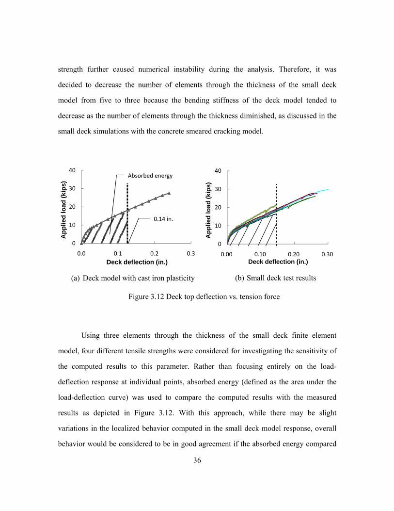
(a) Deck model with cast iron plasticity (b) Small deck test results

Figure 3.12 Deck top deflection vs. tension force

Using three elements through the thickness of the small deck finite element

model, four different tensile strengths were considered for investigating the sensitivity of

the computed results to this parameter. Rather than focusing entirely on the load-

deflection response at individual points, absorbed energy (defined as the area under the

load-deflection curve) was used to compare the computed results with the measured

results as depicted in Figure 3.12. With this approach, while there may be slight

variations in the localized behavior computed in the small deck model response, overall

behavior would be considered to be in good agreement if the absorbed energy compared

0

10

20

30

40

0.0 0.1 0.2 0.3

Ap

plie

d lo

ad (

kip

s)


0

10

20

30

40

0.00 0.10 0.20 0.30

Ap

pli

ed lo

ad (

kip

s)


0.14 in.

Absorbed energy

37

well between the tests and the simulations. For this particular study, a limiting deflection

of 0.14 in. was used when computing the absorbed energy. This value was selected based

on an analysis of the simulation results and the collected test data; thus, it was felt that

0.14 in. of displacement was large enough to capture significant nonlinear behavior in the

deflection response over a wide range of possible tensile strengths as shown in Figure

3.11. This figure shows that the initial large change in slope of the load-deflection curve

occurs when the stresses in the elements at the bottom of the deck reach their tensile

capacity as a result of bending in the specimen. Another slope change occurs when the

loading is approximately equal to 30 kips, which is due to the breakout failure of concrete

surrounding a shear stud. This phenomenon, however, was taken into account by the

mechanical behavior of the connector elements that were incorporated into the model to

represent a shear stud embedded into the deck through a haunch. Thus, for the purposes

of evaluating the concrete model, a limiting deflection of 0.14-in. was selected so that the

computed response, at least for the cases of tensile strength considered, would remain

less than the tensile capacity of the shear stud connections in the model. A detailed

discussion of the connector element behavior is presented in Section 3.3.3.

Figure 3.13 shows the differences in the absorbed energy between the finite

element simulations and the experimental results. The differences in absorbed energy

were normalized by the average absorbed energy obtained from the test data. When the

tensile strength of the cast iron plasticity model was lowered to 4% of the compressive

strength, the normalized energy difference between the simulation results and the test

data became only 0.29%.

38

Figure 3.13 Normalized energy difference between tests and FE analysis

Figure 3.14 Deflection behavior of calibrated cast iron plasticity deck model

‐10

0

10

20

30

40

50

60

70

4 6 8 10

Ab

sorb

ed e

ner

gy

dif

fere

nce

(%

)

Tensile strength, ft / fc' (%)

0

10

20

30

40

0.0 0.1 0.2 0.3 0.4

Ap

plie

d L

oad

(ki

ps)


test

smeared cracking

cast iron plasticity

39

Figure 3.14 shows the deck deflection response of the small deck model using this

tensile strength and the mesh density described above (i.e., three elements through the

thickness). Its general deflection response shows excellent agreement with the test

results. Therefore, the tensile strength was assumed to be 4% of the compressive strength

for the concrete material used in the finite element simulations, and this tensile strength

was also used to construct full-scale bridge models. As stated previously, the small deck

simulation results were affected not only by material parameters such as the tensile

strength but also by the mesh density of the model. Furthermore, the tensile strength and

mesh density for the full-scale bridge model were selected based on the particular

bending behavior observed in the damaged twin box-girder bridge tested during this

research project. Therefore, the tensile strength and the mesh density selected for this

research may not be suitable for other types of bridge slabs or concrete structures.

3.3.3 Shear stud and haunch

A haunch as shown in Figure 3.2(b) is typically used in bridge construction to

help maintain a uniform thickness of the concrete deck. One potential drawback with the

use of a haunch, particularly as it relates to the current study, is that it can reduce the

penetration length of a shear stud into the deck. Such reduced penetration of the stud

could limit the available shear and tensile capacity of the connection between the

concrete deck and the steel girders. For this reason, the AASHTO LRFD Specification

(2007) requires that shear connectors penetrate at least 2 in. into the deck, and the

TxDOT Bridge Detailing Manual (2001) limits the maximum haunch height to 3 in. when

there is no reinforcement in the haunch region.

Shear studs installed on the top flange of a steel box girder provide a mechanical

connection between the girders and the concrete deck for the primary benefit of

40

transferring horizontal shear forces. The transfer of these shear forces leads to the

development of composite action between the steel girders and the concrete deck.

Chemical bonding and friction between the top flange of a girder and the deck might also

provide limited load-transferring capability, but they were not considered in this study

due to their limited strength and the uncertainty in computing their contributions.

Therefore, only mechanical interaction between the shear studs and the concrete deck

were considered in the finite element bridge models developed for this research.

In the redundancy evaluation of a twin steel box-girder bridge, the assumed

damage level was the full-depth fracture of one of the girders (i.e., fracture of the bottom

flange and webs of one girder). Once the assumed damage was induced to the bridge

finite element model, the shear studs could be required to carry significant tension forces

due to the self-weight of the steel girder and the transverse bending of the concrete deck

resulted from the fracture. If the tension force in the studs becomes too large, it could

cause a tensile failure to occur between the concrete deck and the steel box girders. Such

a failure might be attributed to yielding of the stud or breakout of the concrete. Therefore,

bridge models were constructed in such a way that connector elements imitating the stud

connections could capture the tension failure behavior. Mechanical properties and failure

mechanisms of the connector elements are detailed in the following paragraphs.

3.3.3.1 Shear strength and load-slip behavior

Topkaya (2002) investigated the ultimate shear strength and load-slip behavior of

shear studs experimentally. Based on push-out tests, he proposed the ultimate shear

strength Qu and the load-slip relationship Q as follows:

41

0.3'2.5u sc c cQ A f E Equation 3.3

where Asc = cross-sectional area of shear stud (in.2)

fc’ = concrete compressive strength (ksi)

Ec = elastic modulus of concrete (ksi)

30.03

1 20.03

dQ Q

Equation 3.4

where ∆ = slip of shear stud (in.)

Qd = shear load at 0.03 in. displacement (kip)

Qd is defined as the shear load where the shear displacement becomes 0.03 in.,

and the suggested empirical equation is as follows:

0.3'1.75d sc c cQ A f E Equation 3.5

In the full-scale test bridge, three 5-in. long and 7/8-in. diameter shear studs were

installed in a row transversely on the girder top flanges. For simplicity, the three studs

were modeled with a single connector element to represent the group. For example, the

compressive strength of concrete used in the second and third bridge test simulations was

6.23 ksi; thus, the modulus of elasticity of concrete for this case is 4,500 ksi from

Equation 3.6, which is based on the guidelines in ACI Section 8.5.1 (ACI 318-08).

42

'57000c cE f Equation 3.6

Equation 3.6 is empirically based, and the values of Ec and fc’ must be expressed in psi.

Because the shear stud diameter was 7/8 in. and three studs were grouped as one

connector element, the total area of shear studs is 1.325 in.2, and the ultimate strength is

97.38 kips according to Equation 3.3. Qd is 68.16 kips according to Equation 3.5.

Inserting this value into Equation 3.4, the shear load-slip relationship can be obtained,

and it is plotted in Figure 3.15. Beyond 0.3-in. displacement, where the maximum shear

strength is reached, perfectly plastic behavior was assumed in this study. This shear load-

slip relationship was utilized to define the horizontal response of connector elements used

to represent shear studs at the interface between the steel flanges and the concrete deck.

Figure 3.15 Shear force vs. stud slip

0

20

40

60

80

100

0.00 0.10 0.20 0.30 0.40

Sh

ear

forc

e (k

ips)

Displacement (in.)

fc'=6.23 ksi

fc'=4 ksi

43

3.3.3.2 Tensile strength and load-deflection behavior

Sutton (2007) and Mouras (2008) studied the tensile strength of shear studs

embedded in concrete decks under tension forces. As described in the previous section

(Section 3.3.2.2), they used small deck specimens that were capable of representing

transverse bending of a concrete bridge deck between points of inflection. According to

their test results, all specimens failed through concrete breakout (i.e., yielding of shear

studs was not observed). The tensile strength varied depending on the presence of a

haunch, the length of shear studs, the number of shear studs, and the arrangement of shear

studs (i.e., longitudinally or transversely oriented). To quantify the tensile strength of

shear studs embedded in a reinforced concrete deck, they used an ACI equation (ACI

318-08 Appendix D) developed for anchor strength under tension force. In the case of

specimens with a haunch, tensile strengths calculated using the ACI equation did not

agree well with the measured test data. The variation in measured and calculated values

was attributed to the presence of a haunch in some specimens, which is not considered in

the ACI equation. To account for the haunch effect on the tensile strength of shear stud

connections, Mouras (2008) proposed the following modifications to the ACI equation:

, , , ,N c

cbg g N ec N ed N c N bN co

AN N

A

Equation 3.7

' ' 1.5( )b c c efN k f h

Equation 3.8

'

3h

ef ef h

wh h h

Equation 3.9

44

,min, '

0.7 0.3 1.01.5

aed N

ef

c

h

Equation 3.10

, '

'

1

21

3

ec N

N

ef

e

h

Equation 3.11

where Ncbg = design concrete breakout strength of a stud

or group of studs (lb)

ANc = projected concrete failure cone area of a stud group

(=3 hef wh for wh ≤ 3 hef ) (in.2)

ANco = projected concrete failure cone area of a single stud

(= 9 hef’2) (in.2)

g,N = group effect modification factor

1 stud : 1.00

2 studs spaced transversely : 0.95

3 studs spaced transversely : 0.90

Stud spaced longitudinally : 0.80

ec,N = eccentric load modification factor

ed,N = edge distance modification factor

(=1.0 for ca,min ≥1.5 hef’ )

c,N = cracked concrete modification factor

Cracked concrete where a stud installed : 1.00

Uncracked concrete : 1.25

Nb = concrete breakout strength of a single isolated stud (lb)

kc = 24 (cast-in-place shear studs)

45

hef = effective length of a shear stud in concrete —stud length

excluding the stud head in concrete (in.)

hh = haunch height (in.)

hef’ =effective stud length embedded into concrete slab(=hef -

hh) (in.)

wh = width of haunch in the cross-section of a bridge span (in.)

ca,min = smallest edge distance measured from center of stud to

the edge of concrete (in.)

eN’ = eccentricity of resultant stud tensile load

To utilize Equation 3.7 for evaluating the tensile strength of a stud connection with a

haunch, careful attention is needed in specifying the problem parameters because many

components in the equation—such as projected failure cone areas (ANc and ANco), concrete

breakout strength of a single isolated stud (Nb), and edge distance modification factor

(ed,N)—are affected by haunch geometries. In addition to those components, two more

modification factors should be considered for the strength evaluation: cracked concrete

modification factor (c,N) and the group effect factor (g,N). The tensile strength

evaluation procedure proposed by Mouras can become computationally intensive due to

the many factors required to be considered in the equation. Alternatively, a simplified

modification of the ACI anchor strength equation developed by author can be used,

which is available in APPENDIX A. In the proposed simplified modification method,

only a haunch modification factor is required to be computed using Equation A.6 for

evaluating the tensile strength of a stud connection with a haunch. This modification

factor is then multiplied by the value computed using the original ACI equation. One

example for a stud connection with three 5-in. studs is available in APPENDIX B.

46

Figure 3.16 Tensile load-displacement behavior of stud connection

In addition to the maximum tensile strength of shear stud connections, load-

deformation data are needed to define the vertical behavior of connector elements under

tension forces. Figure 3.16 shows a typical load-displacement response of shear studs in

tension. The applied load in the load-displacement response is linearly proportional to the

displacement until it reaches the tensile strength. Beyond the tensile strength, the load

quickly drops because of a brittle concrete breakout failure. For simplicity, two lines

were used to simulate the load-displacement response for the vertical behavior of the

connector elements. The two lines were constructed using the displacement Um

corresponding to the tensile strength and the maximum displacement corresponding to

failure. The maximum displacement was selected to be 12 times Um to match the

0

5

10

15

20

0.00 0.05 0.10 0.15 0.20 0.25

Ten

sio

n f

orc

e (k

ips)

Tensile displacement (in.)

Assumed behavior

Test(Sutton,2007)

12Um Um

Ncbg

47

measured test data and to ensure a smooth change of the deflection curve so as to avoid a

numerical convergence failure in the finite element analyses.

0 0.2 0.4 0.6 0.8 1

hef' / hd

0

0.2

0.4

0.6

0.8

15

7000

0 U

m /

(f c

' (hd+

h h))

test(1stud)test(2studs)test(3studs)regression(Eq. 3.13)

Figure 3.17 Displacement at tensile strength

To determine the value of Um, a regression analysis of the data was conducted

using the test results of Sutton (2007) and Mouras (2008). As shown in Figure 3.17, the

displacement Um tends to increase as the effective stud length excluding the haunch

height (hef’), normalized by the bridge deck thickness (hd), increases. The figure also

shows some scatter depending on the number of studs installed in a row. Although the

dependency of Um on the number studs in a row is not clear because of the limited

amount of data available, specimens containing two studs in a row or one stud show

higher deformation at the tensile strength than specimens with three studs. In this study,

48

all bridges investigated—including the full-scale test bridge—had three studs in a row.

Therefore, to reduce the uncertainty in the selection of Um, the cases with two studs in a

row or one stud were excluded from the regression analysis, and only cases with three

studs were used to construct the haunch effect modification factor in Equation 3.13.

'

,

( )

570000c d h

m h U

f h hU

Equation 3.12

'

, 3.8 34.6 efh U

d

h

h

Equation 3.13

where Um = relative displacement at tensile strength (in.)

h,U = haunch effect modification factor

hd = deck height (in.)

hh = haunch height (in.)

hef’ =effective stud length embedded into concrete slab

excluding haunch height (=hef - hh) (in.)

In APPENDIX D, a detailed explanation of the procedure used to construct

Equation 3.12 is provided. Additionally, APPENDIX D contains a discussion regarding

the applicability of the haunch effect modification factor (Equation 3.13) to other stud

connections having different numbers of studs in a row.

49

3.3.3.3 Shear strength degradation by tensile failure of stud connection

Based on results from stud pull-out tests, embedded shear studs in a reinforced

concrete deck fail in tension due to the formation of a concrete breakout cone in a zone

surrounding the studs. In cases where a haunch is present and the studs are not deeply

embedded, which is consistent with the full-scale bridge tested at FSEL, failure is

associated with the haunch breaking off from the deck. This mode of failure governs the

tensile strength of the stud connection. After tensile failure of a stud connection occurs,

there is clearly no longer any shear resistance mechanism because the studs are

completely embedded in the haunch that is no longer connected to the deck. This

observation suggests that the shear resistance should be interrelated with the tensile

failure of a stud connection. To achieve this relationship, a linear damage model was

applied to the shear resistance of the connector elements. According to the applied linear

damage model, a reduction in the shear resistance of the connector elements is initiated

when the vertical tension force exceeds the tensile strength of the connector elements.

After damage initiation, damage is assumed to evolve linearly, which reduces the shear

resistance of the studs as deformation increases. Eventually, there is a complete loss of

resistance as shown schematically in Figure 3.18.

To investigate the behavior of a single connector element with the assumed linear

damage model under combined shear and tensile loading, the same displacement

magnitudes were applied transversely (for shear) and vertically (for tension), both acting

on one end node of a connector element. Although a linear damage evolution was

assumed for the shear resistance, Figure 3.19 shows a nonlinear load-deflection response

in the shear load-slip behavior. This response is due to the nonlinear plasticity hardening

rule of the shear studs, which was presented in the previous section.

50

P

mU fUU

effd P

effP

mP

1 effP d P

U

Figure 3.18 Damage initiation and evolution mechanism (Dassault Systemes, 2007a)

Figure 3.19 Single connector element behavior under tension and shear forces

0

10

20

30

40

0 0.1 0.2 0.3

Fo

rce

(kip

s)

Displacement (in.)

Tension

Shear

51

3.3.4 Railing interaction

Under normal loading conditions, the contribution of a reinforced concrete bridge

rail is ignored and not considered to be a structural component for resisting gravity loads

because it has gaps for expansion joints. The primary function of a railing is to provide

safety for vehicles on a bridge. When a bridge is subjected to large vertical and rotational

deformations due to severe damage, however, railing gaps may close. Once such gaps

close, the railing may be able to carry significant forces in the longitudinal direction of a

bridge. This situation is similar to having a deep beam at the edges of the bridge.

In this study, a simplified modeling approach was used to account for the

possibility of the engagement of rail sections. Rather than performing a direct contact

analysis, nonlinear springs in expansion joint gaps were used. For a direct contact

analysis, a refined mesh density is needed at contact surfaces in order to obtain suitably

accurate results, and convergence problems frequently arise when the analysis includes

nonlinear material properties (Dassault Systemes, 2007a). In modeling a full-scale bridge,

significant effort and computational resources are needed to create a finite element model

with appropriate mesh refinement in regions where contact can occur. Furthermore,

convergence problems associated with small contact regions can lead to excessively long

run times and potentially prevent an analysis from running to completion due to

convergence issues. For these reasons, spring elements inserted between rails were used

to simulate the potential railing engagement through expansion joints. Once the rails

engage, it is possible that limited shear forces may be transferred due to friction, but this

effect was ignored in the finite element models developed for this research. It was

assumed that spring elements in expansion joint gaps transferred only normal forces.

Before the gaps in the railings become completely closed, no normal forces

should develop in the spring elements. This behavior is captured in the spring load-

52

deflection behavior shown in Figure 3.20. This figure shows that the spring elements

resist only compression forces once the deflection exceeds 3/4 in., which was the initial

gap distance of the rails in the test bridge and the value specified by TxDOT. Beyond the

3/4-in. deflection, a stiffness corresponding to the initial concrete stiffness was assumed

for the spring element to simulate railing contact. The specific stiffness value is not very

important, but it must be large enough to cause a large increase in force; however, it must

not be so large as to lead to numerical inaccuracies in the conditioning of the structural

stiffness matrix. The value selected provided reasonable results, and the computed

response was not very sensitive to variations in the selected stiffness value.

34 in

f

Figure 3.20 Spring element behavior between rails

In the following chapter, modeling procedures for simulating the assumed damage

and loading scenarios for redundancy evaluations and for estimating the remaining load-

53

carrying capacity of a twin box-girder bridge are introduced. The full-scale bridge

fracture tests were conducted according to these damage and loading scenarios. The

computed results are compared with measured test data to verify the validity of the

modeling approach developed for this study.

54

CHAPTER 4: BRIDGE FRACTURE TEST AND SIMULATION

4.1 INTRODUCTION

The full-scale bridge that was used in the experimental testing program (Figure

4.1) had been in service as an HOV lane near the intersection of Interstate I-10 and Loop

610 in Houston, Texas. Because of a highway expansion project, this bridge was removed

from service, and TxDOT made the steel box girders to the research project in 2005. The

steel box girders were transferred to the Ferguson Structural Engineering Laboratory at

the University of Texas at Austin, and the deck and bridge rails were reconstructed.

Detailed reconstruction procedures and geometries of the test bridge are available in

Barnard (2006). After the reconstruction of the test bridge, three separate tests were

performed on the full-scale bridge. The experimental testing program was extensive and

required the development of several unique testing procedures. Below, a brief overview

of the testing program is given. Detailed information describing each of the tests and the

measured data that were collected are available in Neuman (2009).

The purpose of the first bridge fracture test was to investigate how the sudden loss

of the bottom flange of one girder in the bridge affected bridge performance. A rapid

failure of the bottom flange of the exterior girder, which simulates what is expected to

occur during a fracture event, was achieved using a linear-shape-charge explosive to cut

through the complete width of the bottom flange at the midspan. The second test was

conducted to determine whether the bridge could sustain the sudden potential energy

release of a specified live load and the bridge self-weight in a damaged condition (bottom

flange and 83% web removal of exterior girder). For the rapid release of the loads, a

temporary truss support was placed in a prearranged location beneath the bridge’s bottom

flange, and then the web was cut with a torch from the bottom flange to a point

55

approximately 10 in. below the top flange. The temporary truss support was designed to

rapidly release the load it was carrying by severing a tension tie using an explosive in a

similar fashion as the first test. The third test was performed to investigate the reserve

load-carrying capacity of the damaged bridge and the contributions made by individual

bridge components to the overall capacity of the system. To apply loads incrementally in

the experiment, road base was placed on the deck along with concrete blocks. Loading

continued until the bridge collapsed.

Figure 4.1 Full-scale test bridge

56

4.2 FIRST BRIDGE TEST (BOTTOM FLANGE REMOVAL)

4.2.1 Test procedure

The first bridge test was performed to investigate how the bridge responds when

the bottom flange of one girder suddenly fails as might be expected if a fracture were to

occur. The bottom flange is currently classified as a fracture-critical member in the two-

girder bridge system. An explosive was used to cut the bottom flange extremely rapidly

to imitate the sudden loss of the whole bottom flange of one girder (east side girder) at

the midspan as shown in Figure 4.2. For safety purposes, the explosive was encased in a

blast shield, which was attached underneath the bottom flange of the east girder and

tethered to a concrete block placed under the bridge. Other concrete blocks (in the form

of prestressed concrete girders) intended to simulate the AASHTO standard HS-20

design truck load were placed on the deck so as to cause the maximum positive bending

moment at the damaged location. Detailed descriptions of the bridge test setup and the

results that were collected have been reported by Neuman (2009).

Figure 4.2 First bridge fracture test (bottom flange removal by explosion)

Blast shield

57

4.2.2 Simulation procedure

The finite element simulation procedure for modeling the response of this bridge

fracture test can be divided into three main analysis categories: bridge construction, load

application, and simulation of bottom flange fracture, as shown in Table 4.1. The analysis

steps in the bridge construction category are intended to incorporate load histories

through the erection and construction process in which the deck acts non-compositely

with the girders. For the first analysis step, all of the deck, railing, and rebar elements—

except girder elements—were deactivated to simulate the non-composite section behavior

of the bridge. During bridge construction, only the steel box girders resisted the deck and

railing weight before the concrete deck hardened. Therefore, deck and railing elements

were removed using the element deactivation technique in ABAQUS/Standard v6.7 to

simulate non-composite section response because the deactivated elements have no effect

on the mass and the stiffness of the system. After deactivating these elements, equivalent

pressure loads for the self-weight of the deck and railing were evenly applied on the

girder top flanges. As a result, the applied loads on the girder top flanges were resisted

only by the steel girders.

The deactivated elements maintain their initial node locations when they are

deactivated. The node locations of deck and railing elements need to be shifted, however,

so that they deform consistently with the girders because uncured concrete flows freely

before it is hardened. For this reason, dummy elements for the deck and railing were used

to follow such node location shifts. The dummy elements shared the same nodes with the

original deck and railing elements, but they had very low stiffness (10-4 × concrete

stiffness) and were almost without mass (10-9 × concrete density) so as not to affect the

bridge stiffness and weight. As a result, because the original deck and railing elements

were deactivated and an equivalent pressure load was applied to the top flanges of the

58

girders, the deck and railing nodes deformed freely, following the girder deflection due to

the dummy elements. After this procedure, the deck and railing elements were

reactivated, without strain changes, in the deformed position to simulate the hardened

concrete, and the equivalent pressure load was removed.

Table 4.1 Simulation procedures for first bridge fracture test

Bridge construction1. Deactivating deck, railing, rebar elements and applying gravity

to girder2. Applying deck, railing, and rebar weight on the top flange 3. Activating deck, railing, and rebar elements with gravity

and removing the weight on the top flange4. Deactivating external cross frame elements and dummy

elements

Applying truck live load1. Applying truck load (concrete blocks)

Dynamic loading1. Deactivating elements connecting the girder fracture

Sta

tic

Dyn

amic

The truck live load, simulated using concrete blocks in the bridge test, was

applied to the top nodes of the deck using concentrated loads in the finite element model.

These concentrated loads had the same axle spacing as the concrete blocks used during

the test. For the bottom flange cutting, the fracture path was predefined on the bottom

flange of the east girder, as shown in Figure 4.3. The selected damage location was at the

midspan because this location is where the maximum positive bending moment is caused

by a moving vehicle in a simply supported bridge. Shell elements adjoining the

predefined fracture path shared duplicate nodes. These independent nodes were initially

59

joined by connector elements (CONN3D2) with weld properties to mimic the intact

condition of the bottom flange. The cutting of the bottom flange was simulated, therefore,

by removing the connector elements using the element deactivation technique. The

removal of the connector elements was sudden, as was the explosive damage inflicted

during the first bridge fracture test. Computationally, this step was carried out using a

transient dynamic analysis with a “step-amplitude” loading in ABAQUS/Standard v6.7.

Figure 4.3 Predefined bottom flange fracture path

4.2.3 Bridge test and simulation results

After the first bridge fracture test, it was observed that the bottom flange was

severed completely along its width and through its depth. The fracture, however, did not

propagate into the webs as shown in Figure 4.4. Despite the bottom flange fracture of one

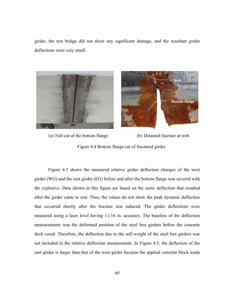
60

girder, the test bridge did not show any significant damage, and the resultant girder

deflections were very small.

(a) Full cut of the bottom flange

(b) Detained fracture at web

Figure 4.4 Bottom flange cut of fractured girder

Figure 4.5 shows the measured relative girder deflection changes of the west

girder (WG) and the east girder (EG) before and after the bottom flange was severed with

the explosive. Data shown in this figure are based on the static deflection that resulted

after the girder came to rest. Thus, the values do not show the peak dynamic deflection

that occurred shortly after the fracture was induced. The girder deflections were

measured using a laser level having ±1/16 in. accuracy. The baseline of the deflection

measurements was the deformed position of the steel box girders before the concrete

deck cured. Therefore, the deflection due to the self-weight of the steel box girders was

not included in the relative deflection measurement. In Figure 4.5, the deflection of the

east girder is larger than that of the west girder because the applied concrete block loads

Web

Bottom flange

61

(used to simulate an HS-20 truck) were biased transversely toward the east girder to

create the worst-case loading scenario on the fractured girder (Neuman, 2009).

Figure 4.5 Girder deflection of intact and fractured girder

According to the surveyed data, the east girder deflected downward 5.56 in. at its

midspan (relative to the baseline) when the concrete blocks were loaded and before the

bottom flange fracture occurred. The resulting additional deflection of the east girder was

only 0.08 in. after its bottom flange was fractured. This result is inconclusive, however,

as it is within the specified accuracy of the laser level. Moreover, the deflection surveys

were conducted on different days and at different times, which could mean that different

environmental conditions affected the bridge deflection (i.e., temperature gradient change

could affect the bridge deflection measurements). Therefore, the measured additional

‐6.0

‐5.0

‐4.0

‐3.0

‐2.0

‐1.0

0.0

0 20 40 60 80 100 120

Ver

tica

l def

lect

ion

(in

.)

Distance from south (ft.)

Before fracture (WG)

After fracture (WG)

Before fractute (EG)

After fracture (EG)

62

deflection might not be caused solely by the bottom flange fracture of the east girder.

Nonetheless, the measured deflections and post-test observations of the bridge indicate

that the fracture of the bottom flange of the exterior girder caused limited damage to the

overall load-carrying capacity of the bridge.

Figure 4.6 Fractured girder deflection after bottom flange removal

The finite element simulations gave girder deflections that were similar to those

obtained from the surveyed data. Figure 4.6 compares the measured deflections of the

fractured girder with those predicted by the finite element model following the fracture of

the bottom flange. The predicted deflection at the midspan by the finite element model

was 5.23 in., which was slightly less than the measured deflection of 5.64 in. Considering

the accuracy of the laser level and the possibility for environmental conditions to affect

‐6

‐5

‐4

‐3

‐2

‐1

0

0 20 40 60 80 100 120

Ver

tica

l def

lect

ion

(in

.)

Distance from south support (ft.)

Measurement

FEM

63

the measured deflections, however, the prediction by the finite element model was

considered to be acceptable.

4.3 SECOND BRIDGE TEST (BOTTOM FLANGE AND WEB REMOVAL)


The purpose of the second bridge test was to investigate whether or not the FSEL

bridge could sustain a simulated dynamic loading following a nearly full-depth fracture

of the exterior girder (the east side girder). The applied damage and loading conditions

were similar to those described in Chapter 2 for the redundancy evaluation of a twin steel

box-girder bridge. The only difference was the level of damage that existed prior to the

test. In the experiment, 83% of the east girder’s web was cut, rather than the total web,

because of safety issues. For the bridge test, in order to apply the additional web damage

without the loss of the gravitational potential energy of the bridge, a temporary truss

support was installed under the fractured girder. Then, the bottom flange fracture made in

the first bridge fracture test was manually extended to the inside and outside webs of the

east girder using an acetylene torch. Figure 4.7 shows the condition of the bridge after the

webs had been cut.

After inducing the additional web damage, concrete blocks were placed on the top

of wooden blocks on the deck to represent truck axles. The concrete blocks were intended

to simulate the AASHTO HS-20 truck load, but it had a slightly different total weight—4

kips higher than the HS-20 truck. Figure 4.8 shows a schematic of the concrete block

loading configuration used in the second bridge fracture test. The assumed spacing of

axles was 14 ft., and the middle axle was positioned at the midspan to cause the

maximum vertical bending moment at the fracture location. The transverse location of the

64

concrete blocks was biased toward the east girder side so that the axle (wooden block)

corners were placed 2 ft. away from the east railing. This configuration was intended to

simulate the worst-case loading condition that could be achieved by a single truck on the

test bridge.

(a) Second bridge test setup (b) Manually extended cut to webs

Figure 4.7 Temporary support and web cutting

Figure 4.8 Simulated truck live load configuration (AASHTO HS-20)

Temporary support

Wood block

E W

E

W

65

Figure 4.9 Temporary truss support and explosive setup

Figure 4.10 Second bridge fracture test (bottom flange and 83% web removal)

For the second bridge fracture test, the temporary truss support was designed so

that it could collapse nearly instantaneously without interfering with the response of the

bridge as it deflected downward. The temporary truss support designed by Neuman

(2009) satisfied these requirements successfully. It became structurally unstable once

horizontal ties, as shown in Figure 4.9, were severed by explosive contact charges, and it

quickly dropped down before the bridge girder deflected. This behavior was clearly

observed in the high-speed video recording of the test; captured still images from the

high-speed video are shown in Figure 4.10.

Horizontal truss member

Explosive

Blast shield

66


To simulate the damage and loading scenario used in the second full-scale bridge

fracture test, the finite element analysis followed procedures similar to those in the first

bridge test. The finite element simulation of the second bridge test was composed of three

major analysis steps, as described in Table 4.2: bridge construction, applying temporary

boundary conditions and girder damage, and removing the temporary boundary

conditions.

Table 4.2 Simulation procedures for second bridge fracture test

The bridge construction step was used to incorporate loading histories associated

with non-composite behavior before casting the concrete deck, as discussed in the first

bridge fracture test simulation procedure. For the next step, temporary boundary

conditions were applied to the bottom flange, spanning 5 ft. and centered on the midspan

of the east girder where the temporary truss supports were placed. The temporary

67

boundaries constrained the vertical translation of the east girder while the bottom flange

damage, the web damage, and the simulated truck live load were applied to the

simulation model. To incorporate damage on the east girder, connector elements initially

binding separated nodes along a predefined fracture path were deactivated. The

predefined fracture path and temporary boundaries under the bottom flange are shown in

Figure 4.11. The truck live load represented by the concrete blocks in the bridge test was

simulated with concentrated forces acting on the bridge deck.

Figure 4.11 predefined fracture path in east girder

After the loading step of the truck live load, the temporary boundaries were

eliminated to simulate the sudden removal of the temporary truss supports in the bridge

fracture test. To computationally achieve dynamic loading effects caused by the abrupt

removal of the temporary supports, a transient dynamic analysis was conducted with a

“step-amplitude” loading condition.

68


After the second bridge fracture test, visual inspections were conducted to

investigate the overall condition of the bridge. During the initial inspections, the only

damage observed included tensile cracks on the deck and crushed cover concrete on the

top of the east railing at the midspan. Analytical models of the deck response (Samaras,

2009) and finite element simulations, however, predicted that extensive stud tensile

failures would occur along the inside of the fractured girder. For this reason, the

corrugated metal deck spanning between the girders and used as formwork during the

construction of the deck was removed to inspect the stud connections closely, and it

revealed that a large amount of haunch separation along the inside of the fractured girder

had in fact occurred (Figure 4.12 (a)). Along the outside of the fractured girder, both

longitudinal and diagonal cracks were observed where the studs connected with the

concrete deck, as shown in Figure 4.12 (b). These cracks developed near the midspan. As

indicated by the figure, haunch separation on the inside of the girder was more severe

than on the outside.

(a) Fractured girder: inside (b) Fractured girder: outside

Figure 4.12 Haunch separation of fractured girder

69

Figure 4.13 Haunch separation along bridge span

In the test bridge, haunch separation was initiated by stud tensile failure near the

midspan of the bridge. As the tensile failures propagated along the bridge span, the

haunch started to separate from the concrete deck of the fractured girder. Figure 4.13

shows the predicted length of haunch separation along the inside of the fractured girder

(FG-In) and along the outside (FG-Out); the figure also shows the measured haunch

separation along the inside of the fractured girder. A comparison of the results indicates

that the finite element model over-predicted the separation length along the inside of the

fractured girder—96 ft. predicted compared to 67 ft. measured. Along the outside of the

fractured girder near the midspan, cracking in the haunch spanned 14 ft., but the cracking

pattern was irregular, as shown in Figure 4.12(b) (i.e., diagonal and longitudinal cracks

were both observed). This cracking pattern suggests that the outside haunch failed due to

a combination of tension and shear. Because the degree to which haunch separation

occurred along the outside of the fractured girder could not be accurately measured, only

0

1

2

3

4

5

0 20 40 60 80 100 120

Sep

arat

ion

mag

nit

ud

e (i

n.)


FEM (FG‐In)

FEM (FG‐Out)

Measurement (FG‐In)

70

the simulation model prediction is included in Figure 4.13; the predicted separation

length was 32 ft.

Concerning the over-prediction of the haunch separation length, there are various

possible reasons: haunch slope, participation of the metal deck, dynamic effects on

material strength, and potentially others. In the test bridge, the edge of the haunch was

sloped transversely due to the corrugated metal stay-in-place forms used to construct the

deck (Figure 4.14). The presence of such a haunch slope could change the tensile strength

of a stud connection because it reduces the concrete breakout cone size less than does a

haunch with right angles. The strain rate of the dynamic loading could also affect the

tensile strength of a stud connection because material strength is affected by the loading

rate. Figure 4.15 shows the variation in the tensile strength of stud connections as a

function of the loading rate based on tests conducted by Mouras (2008). According to the

test results, when the strain rate reached 30.67 in./in./msec.—the maximum obtained

during the testing program—the tensile strength increased by about 40% over the static

test results. The finite element simulation model, however, did not consider such an

increase in tensile strength caused by the high strain rate; for simplicity and due to a lack

of data, constitutive models used in the finite element simulations were not strain-rate

dependent.

Figure 4.14 Haunch slope in cross-sectional plane

71

Figure 4.15 Dynamic and static stud pullout test (Mouras, 2008)

Figure 4.16 shows the girder midspan deflections as a function of time obtained

from the finite element simulation. The dashed line indicates the vertical deflection of the

intact girder (IG-CL), and the solid line represents the vertical deflection of the fractured

girder (FG-CL); both quantities were obtained from the centerline position of the bottom

flange. To obtain the centerline deflections at the midspan of the bridge, edge deflections

of the bottom flange of each girder were averaged. Because of the simulated girder

fracture and the transversely biased loading position of the live load, the vertical

displacement of the fractured girder was significantly larger than that of the intact girder

(Figure 4.16). It is important to note that haunch separations are included in the vertical

displacements that are plotted because the girder displacements were computed from the

response of the bottom flanges.

0

5

10

15

20

25

30

0.0 0.1 0.2 0.3 0.4 0.5 0.6

Ten

sio

n f

orc

e(ki

ps)

Pull out deflection(in.)

dynamic

static

72

Figure 4.16 Dynamic girder deflection

Figure 4.17 Static displacements of test and simulation

‐12

‐10

‐8

‐6

‐4

‐2

0

0 0.5 1 1.5 2

Ver

tica

l def

lect

ion

(in

.)

Time (sec.)

IG‐CL

FG‐CL

‐10

‐8

‐6

‐4

‐2

0

Fractured Girder Intact Girder

Measurement FEM

73

During the bridge test, an attempt was made to measure the dynamic displacement

of the fractured girder at its midspan using a string potentiometer attached to the center of

the bottom flange, but the string potentiometer was damaged from the explosion used to

collapse the temporary truss supports. Consequently, displacements of the bottom flanges

were measured after the test bridge came to rest; these static displacements were

compared with those obtained from the finite element simulation. Displacement values

from the finite element model were obtained by averaging the peak dynamic

displacements after three periods of oscillation (Figure 4.16). This approach was taken

because it was too computationally demanding to carry the dynamic analyses further in

time, and the results showed significant damping. As a result, taking the average value

after three periods of oscillation was reasonable. Figure 4.17 shows the static

displacement results of the intact and the fractured girders, comparing the measured test

data with the computed values. In the bridge fracture test, the vertical displacement at the

midspan of the intact girder was 4.16 in., and the finite element model predicted a value

that was only 2% higher than the test result. Conversely, for the vertical displacement of

the fractured girder, the measured data and predicted value did not compare closely. The

measured deflection of the fractured girder following the test was 7.02 in., but the girder

deflection in the simulation model was 8.63 in. (23% higher). One reason for such a large

difference between the measured and predicted displacement of the fractured girder can

be attributed to the over-predicted separation length of the haunch in the simulation

model compared with that in the bridge fracture test as discussed previously.

The deflected shape of the reinforced concrete deck transitioned from double

curvature to single curvature during the bridge fracture test and the simulation. Figure

4.18 shows the displacement at the top of the deck across the width of the bridge

following the removal of the temporary supports in the bridge fracture test simulation.

74

Early in time (t = 0.06 sec.), the graph shows that the deck bends in double curvature; as

time progresses, however, the shape transitions to single curvature.

Figure 4.18 Deck displacement at midspan

This transition in the deformed shape was initiated by the tensile failure of the

stud connection on the inside of the fractured girder. As the pullout failure propagated

along the length of the bridge, the bridge haunch separated from the concrete deck,

leading to single curvature bending of the deck. Haunch separation in the bridge cross-

section is schematically depicted in Figure 4.19. Once the haunch of the fractured girder

separated from the deck, the transverse bending stiffness of the deck diminished.

Subsequently, the tensile loading attributed to the fractured girder self-weight had to be

carried by the studs on the outside of the fractured girder, which increased the bending

‐12

‐10

‐8

‐6

‐4

‐2

0

0 5 10 15 20 25

Dec

k d

isp

lace

men

t (i

n.)

Distance from west railing corner (ft.)

t=0.06 sec

t=0.14 sec

Max. displ.

75

moment arm for transverse bending of the deck. Therefore, with a wider separation of the

haunch on the inside of the fractured girder, a larger deflection could be expected in the

fractured girder than what was observed in the test.

(a) Deck deflection before haunch separation

(b) Deck deflection after haunch separation

Figure 4.19 deck deflection shape change caused by haunch separation

76

Figure 4.20 Longitudinal strain response by dynamic loading

Figure 4.20 shows the longitudinal strain as a function of time at the centerline of

the bottom flange of the intact girder at a location 6 ft. away from the midspan. The

strains from the simulation and the bridge test show good correspondence, though the

peak measured strain from the test was 13% higher than the simulation result. During the

second bridge fracture test, it is important to note that the crack induced from the

acetylene torch propagated 1 in. upward on the outside of the fractured girder, but this

crack extension was not accounted for in the finite element simulation. Therefore, in the

test bridge, more energy could be released than in the simulation, which may be one of

the reasons why there is a slight discrepancy between the measured and computed results.

Regarding the period of oscillation, there is a slight difference between the measured and

computed values. This difference is most likely attributed to the differences between the

actual damped response of the bridge and the assumptions made about damping in the

0.0E+00

3.0E‐04

6.0E‐04

9.0E‐04

1.2E‐03

1.5E‐03

0.0 0.3 0.5 0.8 1.0

Str

ain

(in

./in

.)

Time (sec.)

S1(test)

S1(FEM)

77

finite element model. In the simulation, 5% damping was assumed—which is a common

assumption for cracked reinforced concrete (Newmark and Hall, 1982)—and the natural

frequency of the first mode of the bridge model was utilized to determine a damping

factor. Because no forced vibration testing of the bridge was carried out, the actual

damped response was not precisely known. Nonetheless, the computed and measured

results show good agreement.

4.4 THIRD BRIDGE TEST (REMAINING CAPACITY EVALUATION)


The third bridge test was performed to determine the ultimate load-carrying

capacity of the FSEL bridge in its damaged state. It should be noted that no attempts were

made to repair the bridge following either of the first two tests. The concrete blocks used

to simulate the truck live load in the second bridge fracture test were rearranged for the

third test, and one additional concrete block was utilized to create a bin that could

accommodate the road base that was used to incrementally load the bridge (Figure 4.21).

Accordingly, the total weight of the concrete blocks in the third bridge fracture test was

82.1 kips. Figure 4.21 shows a schematic of the concrete block configuration on the

bridge deck. The concrete blocks were symmetrically arranged about the bridge midspan,

and they were transversely biased toward the fractured girder. Wooden planks used to

support the concrete blocks were located 2 ft. away from the east railing.

78

Figure 4.21 Concrete block configuration on bridge deck

While positioning the concrete blocks on the deck, the crack in the outside web of

the fractured girder propagated toward the top flange, as shown in Figure 4.22. Prior to

this crack propagation, the crack was sharpened by the 1-in. crack extension upward from

the point where the torch cut terminated during the second bridge fracture test. The total

loaded weight of the concrete blocks was 40.9 kips when the crack propagation occurred.

This sudden crack propagation caused the bridge to vibrate, but the small oscillations

quickly subsided. The crack on the inside web did not propagate when the concrete

blocks were placed on the bridge. Though the weight and positioning of the blocks

represented a less severe load case than the bridge withstood during the second test, it is

believed that the cold weather present while the blocks were being placed during the third

bridge test contributed to the crack extension (Neuman, 2009).

79

Figure 4.22 Crack propagation in fractured girder outside web

(a) Incremental loading (b) Collapsed bridge

Figure 4.23 Loading process and bridge collapse in third bridge fracture test

Crack propagation

Sharpened crack tip in 2nd test

80

Figure 4.23(a) shows the loading process used during the third test on the FSEL

bridge. Road base, consisting primarily of gravel and dirt, was placed in an air-operated

lift bucket using a small backhoe. The lift bucket was attached to the lifting hook of a

crane. Once the bucket was filled, the weight of the road base was measured using a load

cell attached to the end of the crane hook. After the crane lifted the bucket and the weight

was recorded, the lift bucket was positioned above the bridge, and the road base was

placed inside the concrete bin located on the bridge deck (Figure 4.21). When 258.3 kips

of road base was loaded onto the bridge, there was no more space available inside the bin.

Therefore, it was decided to apply additional road base between the concrete blocks and

the east railing. The bridge finally collapsed when the total applied load of the concrete

blocks and road base reached 363 kips—more than five times the legal truck load—as

shown in Figure 4.23(b).


The third bridge test simulation consisted of three main steps similar to those in

the previous bridge test simulations, as presented in Table 4.3. Recall that for the second

bridge fracture test, approximately 83% of the full height of the web was cut using an

acetylene torch. During the second test, a fracture initiated from the top of the cut on the

outside web of the fractured girder and extended approximately 1 in. upward toward the

top flange. While applying the concrete blocks for the third bridge test, this web crack

extended to the top flange. The inside web crack also propagated up from the crack

manually induced prior to the second test, and this cut extended through the entire depth

of the web during the third bridge test. For these reasons, it was assumed that the entire

web depth of the fractured girder was fractured. Accordingly, the web connector elements

along the predefined fracture path were removed through the entire web height for the

81

third bridge test simulation. Because the loading was incremental, the connector elements

binding separated nodes along the predefined crack path were statically deactivated from

the bottom flange to the top flange.

Table 4.3 Simulation procedures for third bridge fracture test

After removing the web connections, the weight of the concrete blocks and the

road base were applied to the bridge using pressure forces placed consistently with the

bridge test as shown in Figure 4.24. When 258.3 kips of road base was placed inside the

concrete bin during the third bridge test, there was no more space available to

accommodate any additional material inside the bin. Consequently, additional road base

was placed outside the bin between the east railing and the concrete block forming the

eastern edge of the bin as shown in Figure 4.24(c). To match the loading location of this

82

additional road base, the pressure load for the additional road base was applied between

the east railing and the concrete block as shown in Figure 4.24(d).

(a) Concrete block and load base

(b) Simulated pressure load

(c) Additional road base

(d) Simulated additional load

Figure 4.24 Applying concrete block and road base load

For simulating the last step of applying the road base, a dynamic analysis was

conducted using a ramped-loading condition; this approach was not intended to account

for any dynamic loading effects associated with placing the road base. During the last

CONCRETE BLOCK

ROAD BASE PRESSURE

ADDITIONAL ROAD BASE

83

analysis step, various local component failures were expected to occur, such as concrete

cracking or crushing, haunch separation, and so on. Although those component failures

might not necessarily mean collapse of the test bridge, they could cause computational

problems with the static analysis procedure, potentially resulting in an analysis failure

due to numerical convergence problems. Therefore, a dynamic analysis with a ramped-

loading condition was used to avoid such numerical problems.


Data collected from the third bridge test were used to determine the ultimate

strength of the bridge and the contribution made by each bridge component in resisting

the applied loads. It was observed that the shear studs and the concrete deck had

important roles in redistributing the applied loads to undamaged regions of the bridge.

The rails also redistributed loads and initially reduced the deflection of the fractured

girder before stud pull-out failures occurred. The finite element model developed for this

research successfully captured the progressive bridge component failures that were found

in the bridge fracture test and closely predicted the measured collapse load.

4.4.3.1 Failure sequence of the bridge

With the exception of the haunch separation along the outside of the intact girder

near midspan, the simulation model predicted failure modes consistent with those

observed in the bridge test. In Figure 4.25, the failure sequences predicted by the

simulation and those observed during the bridge test are compared at each prominent

component failure event. The failure sequence leading to the collapse of the bridge

initiated with the concrete deck cracking due to transverse bending. As the loading

84

continued, extensive tensile cracking started to form on the top of the concrete deck

above the inside top flange of the intact girder and propagated along the bridge span.

While the bridge continued to deform under the applied loads and transverse bending

increased across the width of the deck, the demand on the shear studs along the inside of

the fractured girder exceeded the tensile strength, leading to extensive tensile failures of

stud connections on both top flanges of the fractured girder. As the tensile failures

propagated along the bridge span, the inside haunch of the fractured girder began to

separate from the bottom of the deck near the midspan of the bridge. While the separated

haunch length along the inside of the fractured girder kept extending over the bridge

span, the bridge deck experienced large deformations near the midspan, and the

expansion joint at the top of the east railing closed over most of its height. Because of the

contact forces acting over the depth of the expansion joint of the east rail at the midspan

location, crushing of cover concrete became pronounced. As the east railing began to

pick up loading and started to crush, the haunch separation along the inside of the

fractured girder continued to extend as did the haunch separation along the outside of the

fractured girder near the midspan. Separation of the haunch along the outside of the

fractured girder was arrested when the separation had propagated to the next expansion

joints (the expansion joint 30 ft. south and the expansion joint 30 ft. north away from the

midspan expansion joint) along the length of the bridge. As the damage in the haunches

of the fractured girder and the east railing progressed, the bottom of the reinforced

concrete deck next to the interior top flange of the intact girder began to crush as a result

of the transverse bending of the deck. Crushing at this location started at the midspan and

propagated in both the north and south directions along the bridge span. This crushing of

the deck was not readily detectable during the test because the permanent metal deck

forms between the girders did not allow the concrete to be observed directly, but the

85

extensive cracking on the top of the deck along a line corresponding to the position of the

interior top flange of the intact girder and deck rotation about this line provided evidence

that the bottom of the deck was crushed. As the applied load approached the maximum

load, shear stresses along the haunch on the outside of the fractured girder increased, and

bridge collapse eventually occurred when a shear failure took place over the entire length

of the outside haunch of the fractured girder.

(a) Tensile cracking on top of the deck above IG-In top flange

(b) Haunch separation along FG-In haunch

86

(c) Railing crushing from top

(d) Deck hinge formation along IG-In top flange

(e) Shear and tension failure of shear studs along FG-Out haunch

87

(f) Bridge collapse

Figure 4.25 Bridge component failure sequence

4.4.3.2 Girder deflection response

The girder vertical deflections measured in the third test are compared with the

simulation results in Figure 4.26. The solid lines show the measured test data, and the

dashed lines show the simulation results. During the bridge test, there was a sudden

vertical deflection in the fractured girder when the applied load reached 160 kips, which

is indicated with the first plateau in Figure 4.26. This sudden increase of the deflection

was caused by the haunch separating from the outside of the fractured girder. The haunch

separation initiated near the midspan and suddenly extended approximately 20 ft. to both

the north and the south (i.e., a total separation of approximately 40 ft.), which is shown in

Figure 4.27. Further separation of the haunch on the outside of the fractured girder did

not occur until the applied load reached approximately 363 kips, which was the

maximum load applied to the test bridge. Unlike the actual test, in the finite element

simulation, the haunch separated gradually along the outside of the fractured girder until

the applied loading reached 308 kips; no further haunch separation occurred until the

applied load reached 413 kips, which was the maximum load the bridge could carry in the

88

simulation. Although the gradual haunch separation in the simulation was not consistent

with the sudden jump observed during the test, the simulation predicted 36 ft. of haunch

separation along the outside of the fractured girder, which is similar to the actual haunch

separation length of approximately 40 ft. observed during the test.

Figure 4.26 Girder deflection response (18 ft. away from midspan)

0

100

200

300

400

500

0 10 20 30

Ap

plie

d lo

ad (

kip

s)

Girder vertical displacement(in.)

IG‐S2(test3) IG‐S2(FEM)

FG‐S2(test3) FG‐S2(FEM)

Haunch separation in FG-Out

Shear and tension failure in Haunch of FG-Out

Shear and tension failure in haunch of FG-Out

Haunch separation in IG-Out

89

(a) Third bridge test (b) Simulation model

Figure 4.27 Haunch separation in FG-Out

Figure 4.28 Slip between the deck and girder top flange along FG-Out

Another prominent feature in the girder deflection response of the test bridge

occurred at the maximum load. When the applied load reached 363 kips, the fractured

girder deflected significantly, and the bridge collapsed. This large deflection was initiated

by the slip between the outside top flange of the fractured girder and the concrete deck, as

0

1

2

3

4

5

0 20 40 60 80 100 120

Sep

arat

ion

mag

nit

ud

e (i

n.)


After girder fract.

170 kips

363 kips

Separated haunch

Deck slip

Diagonal crack

Horizontal crack

FG-Out haunch

90

shown in Figure 4.28. Along the outside haunch of the fractured girder, horizontal cracks

and diagonal cracks were observed, which suggests that failure of the stud connection

was due to the interaction of tension and shear forces. In the simulation model, shear

forces in the connector elements became large along the outside of the fractured girder

when the applied load approached its maximum value of 413 kips. Although the

simulation showed a failure mode that was similar to that of the test bridge, the maximum

load of the simulation model was 14% higher than that of the test bridge.

A notable point for this discrepancy is the shear strength equation (Equation 3.3)

for the connector elements used to simulate the response of the shear studs in the bridge.

As discussed in Chapter 3, Topkaya’s (2002) experimental equations (Equation 3.3 and

3.4) for shear strength and shear load-slip behavior were based on stud push-out tests, and

these equations were utilized in the simulation model for the shear response of the

connector elements. In his tests, Topkaya (2002) used direct shear forces to investigate

the shear load-slip behavior of shear studs embedded in a concrete block. Therefore, his

equation might overestimate the shear strength of stud connections when a tension force

is present. In the simulation model, the shear and tension responses of the connector

elements were dealt with independently, and it was assumed that they did not affect each

other’s strength (i.e., they were uncoupled). The only exception was the shear strength

degradation due to stud tensile failure, as discussed in Chapter 3. This degradation model,

where the tensile failure of a stud connection can lead to shear failure, does not account

for the possibility of the shear strength or the tensile strength being affected by the

interaction of the combined shear-tension force acting on the shear studs. Thus, the shear

strength of a stud connection might be affected if a high tension force—one that is less

than the tensile strength—exists on that connection. Likewise, the tensile strength may be

influenced by the presence of shear forces acting on a stud connection.

91

Besides the possibility of the combined force effect (shear-tension force

interaction) influencing the shear or the tensile strength of a stud connection, the

geometry of the haunch might also affect the shear strength. In the bridge test, deck-slip

failure started at a location about 20 ft. away from the midspan and extended both

northward and southward. It was observed that cracks causing the deck slip were formed

horizontally along the junction where the haunch was connected to the bottom of the deck

and diagonally through the haunch height, as shown in the Figure 4.28. This observation

suggests that the shear failure strength of stud connections could be affected by the

haunch geometry. In the test setup utilized by Topkaya (2002), studs were embedded in a

flat concrete block without a haunch; thus, equations used to predict shear response do

not account for the potential influence of a haunch. In his tests, shear failure of the stud

connection was initiated by concrete crushing around the stud. In the case where a

haunch is present, extensive cracking in the haunch could influence the failure

mechanism—an ultimately the shear capacity—of stud connections.

To investigate the effects of stud shear strength on the ultimate load-carrying

capacity of the bridge, a test simulation with a lower shear strength than the strength

computed from the shear strength equation (Equation 3.3) was conducted. Figure 4.29

shows the simulation results using a reduced shear strength for the connector elements. A

reduction in shear strength of approximately 23% was utilized in the simulation, which

corresponds to the shear strength of a 3/4-in. diameter shear stud (the real shear stud

diameter was 7/8 in.). The simulation with the reduced shear strength predicted a

maximum load capacity that was only 9% higher than the value measured during the

bridge test, which demonstrates the significant impact that a small change in the specified

capacity of the shear studs can have on the prediction of overall bridge capacity.

Although the simulation with the reduced shear strength showed better agreement with

92

the measured results, additional research is needed to develop expressions that can

accurately account for the interaction of shear and tension forces acting on a stud

embedded in a haunch.

Figure 4.29 Girder displacement response with reduced shear strength

The simulation model indicated a failure mode that was not observed during the

test. Unlike the experiment, the simulation showed separation of the haunch and deck

along the outside of the intact girder, leading to an abrupt increase of the fractured girder

deflection as the applied load approached 350 kips. This haunch separation initiated near

the midspan. Once the haunch separated along the outside of the intact girder, the bridge

lost transverse bending resistance, and the concrete deck rotated about the bridge’s

longitudinal axis because the outside and the inside haunches of the fractured girder had

already separated near the midspan prior to the outside haunch separation of the intact

0

100

200

300

400

500

0 10 20 30

Ap

plie

d li

ve l

oad

(ki

ps)

Girder displacement (in.)

IG‐S2(test3) IG‐S2(FEM)

FG‐S2(test3) FG‐S2(FEM)

93

girder. This difference in response between the simulation and test is believed to be

attributed to the underestimated tensile strength of the stud connection computed from the

modified pull-out strength equation (Equation 3.7) as discussed in the previous section.

4.4.3.3 Railing engagement

In the test bridge, the concrete cover on top of the east railing at the midspan

location spalled off during the second bridge test, and the railing remained closed (i.e., in

contact) at the top following the test. As the applied load was increased during the third

bridge test, the concrete at the top of the railing began to crush, and the crushing

propagated downward along the height of the rail. When the applied load reached

approximately 360 kips, a large amount of concrete spalled off, as shown in Figure 4.30.

The depth of spall was approximately 2/3 the height of the railing.

(a) Railing crush during test

(b) Railing crush after collapse

Figure 4.30 East railing crush at midspan

94

To account for the engagement of the rails at the midspan expansion joint,

nonlinear spring elements were used rather than conducting a direct contact analysis. As

discussed in the previous chapter, this choice was made based on computational

efficiency. Figure 4.31(a) shows strain gauges installed on the inside of the east rail, and

Figure 4.31(b) compares the longitudinal strains obtained from the bridge test with those

computed from the finite element simulation. Railing contact occurred progressively

from the top to the bottom of the east rail, which was confirmed by the strain gauge

readings. Figure 4.31 (b) indicates that the simulation successfully captures the

progressive contact of the rails along the railing height; however, the computed strains

start to deviate from the test results after railing contact initiated. It is uncertain why such

discrepancies exist, but they could be attributed to such factors as spalling of concrete

cover, crushing and cracking of the rail concrete, and the presence of non-uniform

contact forces through the width of the railing. The simplified modeling approach used in

this study is not capable of representing these localized effects. After the bridge test, a

large amount of spalled concrete cover was observed on the inside of the east rail at

midspan. This observation suggests that the concrete strain gage readings may not

accurately represent the strain variation in the rails during the test. In addition, it is likely

that the contact forces that existed through the width of the railing were not uniform

because the large deck deflection above the fractured girder caused the rails to rotate

about a longitudinal axis parallel to the bridge span. The simulation model could not

account for these effects because of limitations in the material model that was used to

represent concrete and due to a limited mesh density through the width of the rails.

95

(a) Strain gauge setup

(b) Strain response through railing height

Figure 4.31 Longitudinal strain response along railing height

4.5 SUMMARY

Three sets of tests on a full-scale box-girder bridge were performed at the

Ferguson Structural Engineering Laboratory at the University of Texas at Austin. The

first bridge test involved rapidly severing the bottom flange of the exterior girder using

explosives. The bridge demonstrated excellent performance despite the loss of the bottom

flange. At the midspan position of the fractured girder, the bridge experienced a residual

deflection of less than 1 in., and there was no damage evident to any components of the

bridge. In the second bridge test, the webs of the east (exterior) girder were cut using an

acetylene torch while the bridge was supported by a temporary truss system. The cut

extended from the bottom flange fracture that existed following the first test up towards

the top flanges, with 83% of the web height in a “pre-fractured” condition. With a

simulated HS-20 truck positioned so as to generate the most severe loading, explosives

were used to cause the sudden failure of the temporary truss system supporting the

0

100

200

300

400

‐1.0 ‐0.5 0.0 0.5 1.0

Ap

plie

d lo

ad (

kip

s)Strain (10-3 in./in.)

TOP(FEM)

TOP(test)

14'' from top(FEM)

12'' from top (test)

Strain gauge Railing contact

96

bridge. The failure of the temporary truss supports allowed the sudden release of the

gravitational potential energy of the truck live load and the bridge self-weight. The bridge

successfully sustained the induced damage and sudden release of the loads, though some

of the components were damaged. The last bridge test was conducted to investigate the

remaining load-carrying capacity of the damaged bridge. It sustained approximately 363

kips—more than five times the HS-20 truck load.

The finite element models developed to simulate the bridge tests compared well

with the collected data and post-test observations. Furthermore, the finite element models

successfully captured prominent bridge component failures that were observed during the

second and the third bridge tests. A comparison of the test data with the simulation

models suggested the possibility that equations used to define the behavior of connector

elements used to represent shear studs in the bridge could overestimate the shear strength

of stud connections and could underestimate the pullout strength. According to the bridge

tests and the simulations, prominent failures of the bridge components were the haunch

separation, initiated by tensile failures of stud connections, and crushing of the concrete

rail. Therefore, including such component contributions is crucial for modeling a bridge

to evaluate redundancy. In the next chapter, various factors that can affect the load-

carrying capacity of a fracture critical twin steel box-girder bridge are presented.

97

CHAPTER 5: PARAMETERS AFFECTING BRIDGE LOAD-

CARRYING CAPACITY

5.1 INTRODUCTION

Twin steel box-girder bridges have various load-transferring mechanisms that

allow them to sustain traffic loads even if they suffer a full-depth fracture of one of their

main girders, as demonstrated by the full-scale bridge tests and the corresponding

simulations presented in Chapter 4. To better identify the sensitivity of the research

findings to variations in some of the key performance parameters, finite element

simulations were performed. Investigated parameters included changes in shear stud

length, railing details, variations in horizontal curvature, variations in bridge span length,

and degree of structural indeterminacy (i.e., a bridge with simple spans compared to a

bridge with continuous spans).

To investigate how variations in these parameters affect the load-carrying

capability of these types of fracture critical bridges, incremental load-displacement

analyses were conducted for bridge models that were subjected to initial fractures of the

bottom flange and webs of one girder, which is the same approach previously utilized to

model the response of the FSEL test bridge during the third test (loading scenario B). The

applied external loading consisted of an HS-20 truck positioned at the most critical

location, but each axle load was increased proportionally until collapse was detected or

the load reached five times one HS-20 truck load, whichever came first.

5.2 CONCRETE STRENGTH AND TRUCK LIVE LOAD

The HS-20 standard design truck utilized in this parameter study has a slightly

different configuration than the simulated loading that was used in the third bridge test

98

simulation. An HS-20 truck has three axles spaced 14 ft. apart longitudinally and two

axles spaced 6 ft. apart transversely; the total truck weight is 72 kips. To apply a live load

beyond one truck load, each axle load was increased proportionally relative to its original

axle load. Although the simulated truck live load for the third bridge test (Chapter 4) was

intended to represent an HS-20 truck loading configuration, it did not have distinct

loading axles because of the manner in which the road base was applied to the test bridge.

The road base was distributed through the inside of the concrete bin and the outside of the

bin between the concrete block and the east railing of the test bridge.

Figure 5.1 Fractured girder deflection at midspan (loading type and concrete strength effect)

To quantify the effects of changes in loading configuration and concrete material

strength on the overall capacity of the test bridge, fractured girder displacements were

0

100

200

300

400

500

0 10 20 30 40 50

Ap

plie

d li

ve l

oad

(ki

ps)


Simulated load, fc'=6.23ksi

HS‐20, fc'=6.23ksi

HS‐20, fc'=4ksi

99

computed for three different cases as shown in Figure 5.1. The displacements shown are

those that occurred due to the applied live load following the girder fracture (i.e., no

displacements due to construction loads or the girder fracture are included). All

displacements shown in subsequent figures consider only the post-fracture displacements.

The solid line in Figure 5.1 shows the result of the simulated live load from the third

bridge fracture test, while the dashed line shows the results for the case when the live

load is changed to an HS-20 truck. As mentioned above, the axle loads for the HS-20

truck load were increased proportionally relative to the original axle loads of one truck.

Therefore, in the figure, a 144 kip load means placing one HS-20 truck on top of another.

Comparing the results of the HS-20 load case and the simulated loading, the HS-20 load

case has a more severe loading effect than the simulated loading used during the third

bridge test. One reason for these results is that the HS-20 loading configuration has a

longer lever arm for transverse bending than the simulated loading because the road base

of the simulated load was distributed over a wider region of the deck than the more

concentrated loading of the HS-20 truck.

In addition to the issue of loading configuration differences, it is important to

consider variations in concrete compressive strengths because of the wide range that has

been used in the bridge industry. According to Russell’s report (2003), specified concrete

strengths used for bridge deck construction varied predominantly from 4,000 psi to 8,000

psi. In order to have consistent evaluations on bridge load-carrying capacities for the

current parameter study, a concrete compressive strength of 4,000 psi was used; when

representing the actual bridge tests described in Chapter 4, measured material strengths

from concrete cylinder tests were specified in the finite element models. The concrete

compressive strength not only affects the bending stiffness of a bridge deck, but

according to Equations 3.3 and 3.8, it also influences the shear strength and the tensile

100

strength of a stud connection (i.e., decreased concrete strength reduces the shear and the

tensile strength of a stud connection). The dotted line in Figure 5.1 is the computed girder

deflection for a bridge model that has a concrete deck with a specified compressive

strength of 4,000 psi. As expected, the results show a lower stiffness and a load-carrying

capacity than the other cases. Consequently, in order to develop conservative estimates of

the remaining capacity of fracture critical twin steel box-girder bridges subjected to the

full-depth fracture of one girder, loads are assumed to be positioned and proportioned

according to the axle loads of an HS-20 truck, and concrete material strengths are

conservatively estimated to be 4,000 psi.

5.3 BACKGROUND INFORMATION ON BRIDGES INVESTIGATED DURING PARAMETER

STUDIES

Four bridge models that differed in span length were utilized to investigate

various parameters affecting bridge load-carrying capacity. Box-girder dimensions and

geometries of these models are presented in Figure 5.2 and Table 5.1. The values in Table

5.1 are representative dimensions at girder fracture locations. These dimensions were

collected from shop drawings provided by TxDOT. Among the four prototype bridges

shown in Table 5.1, three bridges (S200, S170, and C130) are currently in service as the

WOODWAY exit ramp near the intersection of Interstate I-10 and Loop 610 in Houston,

and another one (S120) is the test bridge reconstructed at the Ferguson Structural

Engineering Laboratory at the University of Texas at Austin. In Table 5.1, three models

are simply supported bridges that are labeled with an “S” in the front of the model name,

and the model with the label “C” is a continuous bridge having two equal spans.

101

Figure 5.2 Cross-section view of twin steel box-girder bridge

Table 5.1 Box girder dimensions at fracture location

Model Span

length (ft.)

Box girder dimension

Thickness (in.) Width (in.) Depth (in.) Span/Depth

Bot. flange Web Top flange

S200 200 2.00 0.75 1.75 84.0 86.0 27.9 S170 170 1.50 0.75 1.50 84.0 86.0 23.7 C130 130 0.88 0.50 0.75 84.0 53.2 29.1 S120 120 0.75 0.50 0.64 72.0 57.7 25.0

5.4 BRIDGE COMPONENT CONTRIBUTIONS ON BRIDGE CAPACITY

5.4.1 Stud length and deck haunch

The robustness of stud connections plays an important role in the overall load-

carrying capacity of a bridge because they enable the bridge to maintain composite action

between the steel girders and the concrete deck. Under normal conditions when both

girders are fully intact, the stud connections resist mainly shear forces. In the event that a

girder fracture occurs, however, high tension forces will act on the stud connections of

the fractured girder. During the bridge tests carried out under this research project, such

102

tension forces initiated tensile failures of the stud connections along the fractured girder,

leading to a significant reduction in the transverse bending stiffness of the bridge.

Based on the stud pull-out test results reported by Mouras (2008), the tensile

strength of a stud connection is proportional to the embedded length of a stud into the

deck because a longer length increases the concrete failure cone size surrounding a stud.

The presence of a haunch between the bottom of the deck and the top flanges of the steel

girders, however, reduces the effective embedded length of a stud. In addition to the

embedded length reduction, the haunch also confines the failure cone shape and thereby

reduces the concrete surface area available to resist the applied tension force. Because of

these two factors, the tensile strength of a stud embedded in a haunch is less than it would

be in the case no haunch is present. In spite of these drawbacks, a haunch is frequently

used in bridge construction because it is needed to maintain a uniform concrete deck

thickness. For this reason, the effect of a haunch on the tensile strength of a stud

connection was considered in the bridge parameter studies, and the height of the haunch

was consistently assumed to be 3 in., which is the maximum haunch height allowed by

the TxDOT Bridge Detailing Manual (2001) unless reinforcing in the haunch is provided.

Figure 5.3 shows the tensile strengths of stud connections for different stud

configurations obtained from laboratory tests (Mouras, 2008) along with the predicted

results from Equation 3.7. The tensile strength is plotted against the effective stud length,

hef’, normalized by the haunch width, wh. The variable hef

’ is defined as the length a stud

is embedded into the concrete deck, excluding the haunch height and the stud head. As

shown in Figure 5.3, tensile strength goes up as the effective stud length becomes longer

and the concrete strength increases.

103

Figure 5.3 Tensile strength variation along stud length

Figure 5.4 Girder deflection at midspan (stud length effect)

0

10

20

30

40

0.0 0.2 0.4 0.6 0.8 1.0

Nc

bg

(kip

s)

3hef'/2wh

test (fc'=5.1ksi)test (fc'=6ksi)predicted (fc'=4ksi)predicted (fc'=5.1ksi)predicted (fc'=6ksi)

0

100

200

300

400

0 10 20 30 40

Ap

plie

d li

ve l

oad

(ki

ps)


IG (5in. Stud)

IG (9in. Stud)

FG (5in. Stud)

FG (9in. Stud)

Fractured girderIntact girder

104

To investigate the tensile strength effects of a stud connection on bridge load-

carrying capacity, finite element bridge models excluding rails were studied. Rails were

excluded from these models in an attempt to isolate the effects of the shear stud strength

on overall performance. For these analyses, the assumed concrete strength was 4,000 psi,

and the HS-20 loading configuration was used. Figure 5.4 shows the girder displacements

for bridge models with a span of 120 ft. In this figure, girder displacements of a bridge

model with 5-in. stud connections are plotted with solid lines, and displacements of a

bridge model with 9-in. studs are plotted with dashed lines. This figure shows that the

displacements of both girders are reduced when the stud length is increased, and such

displacement reductions are significant in the fractured girder. This tendency was

consistently observed through simulations of bridge models with other span lengths

(C130, S170, and S200).

A detailed study of the simulation results indicated that such displacement

reductions were related to differences in haunch separation behavior. In all models

studied, prominent haunch separations occurred along the insides of fractured girders,

which resulted in transverse bending stiffness reductions across bridge decks and led to

large increases in the displacements of the fractured girders. The outside haunches of

fractured girders also separated near the fracture locations in the bridge simulation

models. In addition to the transverse bending stiffness reductions, these haunch

separations also reduced the vertical bending stiffness of bridges by removing composite

behavior between the concrete decks and the steel girders. Computed results suggest that

as the haunch separation length increases, bridges will demonstrate reduced stiffness and

larger deflections. Figure 5.5 shows the separated haunch length along the inside of the

fractured girder for a model with 5-in. studs. When a separation magnitude representing

the vertical displacement of a stud connector element exceeded its tensile displacement,

105

Um, computed from Equation 3.12, it was assumed that the stud connection was separated

from the deck. To investigate the separated length of a haunch as a function of the

embedded stud length, haunch separation lengths were plotted against applied live loads

following a girder fracture event. These results are shown in Figure 5.6, where the

separation lengths are normalized by the bridge span length and the applied loads are

normalized by one HS-20 truck load. The 9-in. stud model did not show any haunch

separation along the outside of the fractured girder; thus only the separated length of the

fractured girder inside haunch (FG-in) is plotted in Figure 5.6. The separated haunch

length of the 9-in. stud model is much less than that of the 5-in. stud model which led to a

stiffer response and smaller deflections for the fractured girder in the 9-in. stud model

compared to the model with 5-in. studs.

Figure 5.5 Haunch separation in FG-In (5in. stud model)

0

2

4

6

0 20 40 60 80 100 120

Sep

arat

ion

mag

nit

ud

e (i

n.)

Distance along bridge span (ft.)

Girder fracture

72‐kip live load

Separated haunch length

106

Figure 5.6 Separated haunch length variation along applied load

5.4.2 Railing

Bridge deflections with and without the presence of a railing were investigated

using a TxDOT standard T501 rail as shown in Figure 5.7; this rail was selected because

it is widely used in practice. For models that include rails, expansion joints were placed

above the fracture location to minimize the potential increase in bending stiffness rails

may offer at that location. For consistency with the full-scale test bridge, all finite

element models with rails assumed that expansion joints were spaced every 30 ft. along

the bridge span, and gap openings between rail sections were assumed to be 3/4-in. As

with the models used to represent the FSEL test bridge, spring elements were placed in

the expansion joints to account for potential contact of railing sections in the event that

large deflections caused the expansion joints to close.

0.0

0.2

0.4

0.6

0.8

1.0

0 1 2 3 4 5

Sep

arat

ed le

ng

th/s

pan

len

gth

Applied load/HS-20 truck weight

FG_In (5in. stud)

FG_In (9in. stud)

FG_Out (5in. stud)

107

Figure 5.7 T501 rail of FSEL bridge

Figure 5.8 Deck deflection of fractured girder centerline at midspan

0

1

2

3

4

5

6

0 10 20 30 40 50

Ap

plie

d li

ve l

oad

/ H

S-2

0 tr

uck

wei

gh

t

Deck displacement (in.)

No rail T501

Sudden deflection by haunch separation in IG‐Out

108

Figure 5.8 shows deck displacements of bridge models with 120-ft. spans after the

fracture of one girder plotted against the applied live load normalized by HS-20 truck

weight. The deck displacements correspond to the top of the deck at the centerline of the

fractured girder. Initially, as expected, the bridge model with rails deflects less than the

model without rails; however, the deflection at the maximum applied live load (e.g., live

load equivalent to five HS-20 truck weight) is greater for the model with rails than the

one that does not include rails. A prominent feature shown in the figure is the sudden

increase in the deck displacement for the model that included rails as the applied live load

approached 216 kips. This load is equivalent to three HS-20 trucks. Conversely, a sudden

increase in the deck displacement was not observed in the model without rails.

Figure 5.9 Separated haunch length difference depending on railing presence

0.0

0.2

0.4

0.6

0.8

1.0

0 1 2 3 4 5

Sep

arat

ed le

ng

th /

span

len

gth

Applied load / HS-20 truck weight

FG_In (No rail)

FG_In (T501)

FG_Out (No rail)

FG_Out (T501)

IG_Out (T501)

109

According to the finite element analyses of these two models, the main notable

difference in bridge component failures was the haunch separation along the outside

flange of the intact girder. Such haunch separation was observed only in the bridge model

with rails. Figure 5.9 shows variations in the separated haunch length as a function of the

applied live load. The dashed line with circle markers indicates the haunch separation

length along the outside flange of the intact girder for the bridge model that included

rails. As shown in this figure, the haunch separation increased abruptly when the

normalized load level reached approximately three, which is equivalent to three HS-20

trucks. This haunch separation led to a reduction in the transverse bending resistance of

the bridge deck, allowing a rigid rotation of the deck to take place. Therefore, the deck

above the fractured girder could deflect downward abruptly, as shown in Figure 5.8. In

addition, the difference in the haunch separation length shown in Figure 5.9 indicates that

the separated length is longer on the finite element model with rails than the one without

rails. As discussed in the previous section, bridges are expected to exhibit softer behavior

as separated haunch length increases due to a reduction in the transverse bending stiffness

and the vertical bending stiffness of the bridge. Results presented in Figure 5.9 support

this observation.

A detailed investigation of the response helps explain the results shown above in

which, near the onset of failure (i.e., haunch separation along the outside of the intact

girder), bridge models with rails deflect more than models that do not include rails. Under

low levels of applied load, the bridge model with rails showed a slightly stiffer behavior

in the deck displacement response than the model without rails. When the sudden haunch

separation occurred along the outside flange of the intact girder, the deflection of the

bridge model with rails became larger than the one without rails, and this trend continued

up until the applied live load reached to the equivalent weight of five HS-20 design

110

trucks. To explain this behavior, there is a need to focus on the variations in the haunch

separation length along the outside of the fractured girder; Figure 5.9 shows a noticeable

difference between the T501-rail model and the no-rail model. In Figure 5.9, the length

over which the haunch separates in the no-rail bridge model—plotted with solid lines and

squares—initially increases as the applied load increases, but it starts to decrease once the

loading exceeds a single HS-20 truck (i.e., 72 kips). This behavior was caused by the

localized large deflection of the deck above the fractured girder. Because of the position

of the applied live load, the deck deflection increased at a faster rate than that of the

girder. As a result, the deck and girder move closer to each other, with the deck

eventually supported by the girder. When the girder and concrete deck come together, the

haunch separation distance becomes zero. Conversely, for the case of the finite element

model that included the T501 bridge rail, this reduction and eventual closure of the

haunch separation distance was not observed (Figure 5.9). It is believed that this result is

caused by the engagement of the railing above the fractured girder. Once bridge rail

sections are engaged, rails increase the bending stiffness of the deck because they act like

deep beams at the edge of the deck. The increased bending stiffness reduces the deck

deflection and prevents the deck from coming to rest on top of the fractured girder as was

observed in the bridge model that neglected the presence of the rails. Eventually,

however, haunch separation along the outside flange of the intact girder causes the

displacements in the model with rails to exceed those of the model without rails.

5.5 CURVATURE EFFECT ON BRIDGE CAPACITY

Steel box-girder bridges are frequently used in curved regions of highway

interchanges because of their high torsional resistance. As the radius of curvature of a

bridge decreases, torsional stresses increase due to the eccentricity of gravity loads

111

relative to the line of support. In cases where a bridge is damaged, such as the fracture of

one girder assumed for a redundancy evaluation, bridge curvature may negatively affect a

bridge’s load-carrying capacity because the bridge would lose a significant level of

torsional resistance due to the girder fracture. For this reason, curvature effects were

investigated for bridge models with 120-ft. spans.

Figure 5.10 Shear stress of bottom flange at midspan

Figure 5.10 shows shear stresses (i.e., those associated with torsion) in the bottom

flanges at the midspan location of three bridge models having different radii of curvature:

1.) an infinite radius (i.e., a straight bridge), 2.) a radius of curvature equal to 1365 ft.,

which is equivalent to the full-scale test bridge, and 3.) a radius of curvature equal to 800

ft., which is near the lower limit seen in typical field applications. As expected, higher

shear stresses were observed in curved bridges with smaller radii of curvature than those

‐5

‐4

‐3

‐2

‐1

0

1

0 50 100 150 200 250 300 350

Sh

ear

stre

ss (

ksi)

Applied live load (kips)

Inf. (straight)

1365 ft.

800 ft.

112

in bridges with larger radii of curvature; for all cases considered, the actual magnitude of

these stresses was small. As indicated in Figure 5.11, the vertical displacements of the

fractured girders showed behavior consistent with that of the shear stresses. Although the

bridge curvature does not affect the vertical deflection notably in these cases, the effect

might be significant in cases where the span length is much longer than these models.

Therefore, additional research is needed to clarify the curvature effects on this type of

bridge.

Figure 5.11 Fractured girder deflection at midspan (curvature effect)

5.6 STRUCTURAL INDETERMINACY

Unlike a simply supported bridge, bridges with continuous spans are statically

indeterminate and therefore inherently possess some degree of system redundancy. Thus,

0

100

200

300

400

0 10 20 30 40 50

Ap

plie

d li

ve l

oad

(ki

ps)


Inf. (straight)

1365 ft.

800 ft.

113

if a twin steel box-girder bridge is constructed continuously over multiple supports, its

response following the fracture of one girder can be redistributed to a neighboring girder

as well as neighboring spans—potentially improving its chances to survive a fracture

event more effectively than a simply supported bridge. To investigate the possible

beneficial effects of structural indeterminacy, the post-fracture behavior of the two-span

continuous bridge model (C130), as described in Table 5.1, was analyzed in this study.

Figure 5.12 Normal stress envelop curve along bridge span

In the analysis of the simply supported bridge models described previously, the

girder fracture location was selected to be at the midspan because the maximum positive

bending moment caused by the bridge self-weight and a truck live load occurred at this

location. To determine the location where positive bending moment was maximized by

bridge self-weight and a live load for the continuous span bridge model, a moving load

0

5

10

15

0.0 0.2 0.4 0.6 0.8

No

rmal

str

ess

(ksi

)

Distance from simple support / span length

DL+LL

DL

114

analysis was conducted. Before applying the moving load to the bridge, deck self-weight

was applied on the top flanges of the bridge girders with gravity loading for girder self-

weight (to account for non-composite section behavior), and then the moving load

representing a truck live load was applied by changing its location by increments of 2 ft.

along the bridge span. Figure 5.12 shows the results of the moving load analysis for the

C130 model. The solid line shows the normal stress envelope induced by the bridge self-

weight (dead load, DL) and the moving load (live load, LL). The normal stress was

measured in the bottom flange of the girder for which the simulated fracture was to be

specified. As shown in Figure 5.12, it was found that the maximum normal stress

occurred at 51 ft. away from the simple support, which corresponded to a relative

position of 40% of one span length. Therefore, this location was specified as the fracture

location of the continuous span bridge model.

Figure 5.13 Girder deflection at midspan (continuous span)

0

100

200

300

400

0 10 20 30 40 50

Ap

plie

d li

ve l

oad

(ki

ps)


IG (S120)

IG (C130)

FG (S120)

FG (C130)

Sudden deflection by haunch separation in FG‐Out

115

Figure 5.13 compares girder deflection behavior at midspan of the simply

supported bridge model (S120) and the two-span continuous bridge model (C130). Due

to the differences in cross-section size and other dimensions (Table 5.1), it is not

appropriate to compare the computed results directly. Nonetheless, it is important to

identify differences in the response behavior of these models and to recognize that the

continuous span model had a longer span and a smaller cross-section than the simple-

span model.

Notably different responses were observed between these two models for the

fractured girder deflection behavior, as shown in Figure 5.13. As the applied load reached

approximately 160 kips, sudden haunch separation along the outside of the fractured

girder was observed near the fracture location of the continuous span bridge model. It

was caused by the cantilever action emanating from the interior support side of the

bridge. Because of the position of the assumed fracture location relative to the layout of

this two-span continuous bridge, the far end rested on a simple support that could not

provide such cantilever action. Thus, the interior side that could develop cantilever action

restrained the far side resting on the simple support. This restraint caused the tension

force on the stud connection near the girder fracture location to increase, eventually

causing haunch separation to occur locally near the fracture location along the outside of

the fractured girder.

An interesting observation is that the continuous span bridge model showed fairly

stiff deflection behavior in the fractured girder although it showed the sudden

displacement increase in the fractured girder. T501 rails were added to these two models

because the rails increased tensile forces on the stud connections in the simple-span

model (S120) and led to haunch separation along the outside of the intact girder causing

116

the unstable deflection in the fractured girder under the loading range considered (i.e., 5

times an HS-20 truck load).

Figure 5.14 Girder deflection at midspan (continuous span with T501 rail)

Figure 5.14 shows the analysis results for these two bridge models with the T501

railing. Although the haunch separation along the outside of the fractured girder in the

continuous span bridge model occurred and caused sudden deflections in the fractured

girder, the continuous bridge showed stiffer deflection behavior, particularly for the

fractured girder, than the simple-span bridge. The girder displacement differences

became large after the haunch separation along the outside of the intact girder was

initiated in the simple-span model. Interestingly, such haunch separation along the

outside of the intact girder did not occur for the continuous bridge model. This behavior

0

100

200

300

400

0 10 20 30 40 50

Ap

plie

d li

ve l

oad

(ki

ps)


IG (S120)

IG (C130)

FG (S120)

FG (C130)

Haunch separation in IG‐Out

Haunch separation in FG‐Out

117

may be attributable to the fact that vertical bending resistance could be developed for the

continuous bridge due to the cantilever action even after the fracture of one girder, and

the applied load could be transferred longitudinally along the bridge interior span.

Conversely, in the simple-span model, the applied load was transferred through the

transverse bending behavior of the deck, which caused the increase of the tensile force on

the stud connection along the outside of the intact girder. These results imply that the

continuous bridge has higher post-fracture load-carrying capacity than the simply

supported bridge even though it has a longer span and a smaller cross-section.

5.7 BRIDGE SPAN LENGTH AND DYNAMIC AMPLIFICATION FACTOR

Three simple-span bridges that differed in their span lengths were analyzed to

investigate post-fracture load-carrying capacity as a function of span length. Figure 5.15

shows girder deflection behavior for these bridge models, and it is interesting to note that

the results do not show any significant span length dependency. However, considering

the ratio of span length to steel box-girder depth—values are indicated on top of each

fractured girder deflection plot—the fractured girder deflections increase as this ratio

increases. Intact girder deflections also tended to behave similarly with the fractured

girder until yielding in the bottom flange of the 120-ft span bridge model (S120) was

initiated.

118

Figure 5.15 Girder deflection at midspan (span length effect)

5.8 SUMMARY

In this chapter, the following parameters were investigated to determine their

influence on the load-carrying capacity of a twin steel-box girder bridge: stud length,

railings, bridge curvature, structural indeterminacy, and span length. It was found that the

tensile strength of stud connections played a major role in the post-fracture behavior of

these types of bridges. Results from this research program indicate that the tensile

strength of a stud connection is negatively influenced by the presence of a haunch and

limits the maximum load a twin steel box-girder bridge can carry following the fracture

of one of its girders. T501 bridge railings act as deep beams at the edges of the concrete

deck and can carry substantial loads after their expansion joints close. In the models

studied, their presence initially reduced the deck deflection compared to the models that

0

100

200

300

400

0 10 20 30 40 50

Ap

plie

d li

ve l

oad

(ki

ps)


IG (S120)

IG (S170)

IG (S200)

FG (S120)

FG (S170)

FG (S200)

23.7 27.925

Initiation of IG bottom flange yielding at midspan

119

did not include rails; however, models with rails showed an increase in the tensile forces

acting on stud connections, which resulted in the haunch separating along the outside of

the intact girder near the fracture location. This haunch separation caused the deflection

in the fractured girder to increase abruptly. Another parameter that was varied in the

finite element models developed for this research was the radius of curvature, and the

results showed sensitivity to changes in this value. As the radius of curvature decreased,

deflections in the fractured girder increased. Structural redundancy achieved through a

continuous span bridge positively affected the overall load-carrying capacity of the twin

steel box-girder bridges analyzed for this research. The continuity of the bridge helped it

sustain the applied load without causing haunch separation along the outside of the intact

girder. Finally, post-fracture girder deflections showed a stronger dependence on the span

length-to-depth ratio than the span length itself. As the ratio of span to depth increased,

the fractured girder deflections also increased.

In the next chapter, application of the redundancy evaluation methods described

in Chapter 2 is presented. For the redundancy evaluations, four bridge models were

utilized. Because the finite element results presented in this chapter showed that bridge

rails could negatively affect the load-carrying capacity of a bridge, rails were included in

the investigated bridge models.

120

CHAPTER 6: REDUNDANCY EVALUATION (APPLICATION)

6.1 INTRODUCTION

In Chapter 2, loading scenario A, which entails the sudden full-depth fracture of

one girder in a twin box-girder bridge, was introduced as a basis for evaluating bridge

redundancy. Using this methodology, four bridge models were analyzed to evaluate the

role played by different system parameters in affecting overall performance, and the

results of these analyses are included in this chapter. To numerically achieve the damage

and loading conditions assumed for the redundancy evaluation of these bridges, the same

analysis procedure utilized in the simulation of the second full-scale bridge fracture test

in Chapter 4 was followed.

6.2 BRIDGE MODELING AND ASSUMPTIONS

For the redundancy evaluation of twin steel box-girder bridges described herein,

the same bridge models used in the parametric study presented in Chapter 5 were utilized.

The primary dimensions of these bridge cross-sections are given in Table 5.1. These

models were constructed according to the modeling guidelines (such as element types,

inelastic material behavior, mechanical behavior of a stud connection, and railing

interaction using spring elements) described in Chapter 3. For the deck and the rail

concrete of these bridge models, a compressive strength of 4,000 psi was conservatively

assumed, and a TxDOT standard T501 rail was utilized similarly to the full-scale test

bridge. All of the investigated bridge models utilized stud connections comprised of three

studs in a row as schematically shown in Figure 6.1, and the studs had a diameter of 7/8-

in; however, the stud length and the haunch width differed as listed in Table 6.1. The

haunch height of the prototype bridges varied from 2 in. to 3 in., but a 3-in haunch height

121

was conservatively assumed for all bridge models. Table 6.1 shows resultant shear and

tension strengths of stud connections utilized for the models. For the expansion joints

between rail sections, a 3/4-in. gap distance was assumed, and spring elements were

inserted in the gap to account for railing engagement in all bridge models.

Table 6.1 Primary dimensions and strength of stud connection

Model Stud Haunch

width (in.)

Shear and tension strength (kips)

length (in.)

Spacing (in.)

Shear (Eq. 3.3) Tension (Eq. 3.7)

S200 6 6 18

79.77

18.82 S170 6 4 18 18.82 C130 6 4 14 17.19 S120 5 4 12 12.64

Figure 6.1 Schematic of stud connection with haunch

122

6.3 DETERMINATION OF FRACTURE LOCATION AND ANALYSIS PROCEDURE

The applied damage and loading scenario for the redundancy evaluation of the

prototype bridges was the sudden full-depth fracture of one girder with an HS-20

standard design truck positioned to cause the maximum positive bending moment at the

fracture location. The investigated bridges contained one physical traffic lane; thus one

truck live load was considered. The truck live load (i.e., the HS-20 standard design truck

load) was placed on the deck of each bridge such that the middle axle was positioned at

the fracture location while the axle spacing was assumed to be fixed at 14 ft. The

transverse location of the truck live load was biased toward the fractured girder so that

the axle corners were placed 2 ft. away from the bridge railing.

To numerically simulate the sudden full-depth fracture of one girder, duplicate

nodes were included along the predefined fracture path. Thus, elements of the girder

along the fracture path shared coincident nodes, but these duplicate nodes were not

connected. Instead, the duplicate nodes were initially joined using connector elements

with welding properties to simulate the pre-fracture condition of the girder; later, they

were deactivated to simulate girder fracture along the predefined path. Initially, to

simulate sudden fracture along the predefined fracture path, the connector elements were

deactivated instantaneously. However, this technique resulted in numerical convergence

problems, and analyses failed to run to completion. As a result, the same procedure used

in the simulation of the second full-scale bridge fracture test was used for these analyses.

The detailed analysis procedure is available in Table 4.2.

123

6.4 EVALUATION RESULTS

6.4.1 Dynamic displacement response

The investigated bridges successfully sustained the considered damage and

loading level simulating the full-depth fracture of one girder in a two-girder bridge.

Figure 6.2 shows post-fracture dynamic displacement responses at the girder fracture

locations of these bridge models. As shown in this figure, the maximum girder

displacement induced by the sudden fracture tended to increase as the span length

increased for the simple span bridge models. When the displacements were normalized

by each bridge span length, however, the increasing tendency of the displacement was

dependant on the span-length-to-box-depth ratio rather than the span length itself (Figure

6.3). The continuous bridge model (C130) showed much smaller girder displacements

than any of the simple span models due to the benefit of structural indeterminacy in

addition to the load path redundancy that the bridge possessed. Table 6.2 lists detailed

values of maximum girder displacement results obtained from the finite element

simulations. The listed maximum girder displacements do not include bridge self-weight

(i.e., the displacements by bridge self-weight prior to the girder fracture were not

included).

Although a bridge may possess sufficient strength to sustain a specified level of

damage and loading, excessive displacements that could be a potential hazard to bridge

users could be caused if the level of damage and loading is so large as to induce material

inelasticity or local failures of bridge components. Therefore, the displacement of a

bridge should be checked to determine whether or not a bridge is redundant. The current

AASHTO LRFD bridge design specifications (2007), however, do not provide any

provisions or guidance regarding the displacement limit (based on the ultimate load

capacity of a bridge) that can be utilized for a redundancy evaluation. Ghosn et al. (1998)

124

proposed a displacement limit caused by live load as one percent of the span length based

on engineering judgment, and they defined the displacement limit as a “functionality

limit state”. If the functionality limit state is utilized as the displacement limit for the

redundancy evaluation of a twin steel box-girder bridge, some of the investigated bridges

would not satisfy this requirement. For the judgment of the displacement limit, however,

Ghosn et al. (1998) used a somewhat ambiguous definition based on “the maximum

visible displacement that a bridge user or an observer can tolerate”. The assumed damage

and loading level in this study was intended to simulate the worst-case loading with very

severe damage; thus, the possibility of occurrence would be rare. For such a rare event, it

is questionable as to whether or not an allowable displacement criterion should be based

on maintaining a tolerable appearance. Instead it might be preferable to ensure a level of

protection that allows for the safe evacuation of bridge users. To establish such a

displacement limit, however, additional research is needed.

Table 6.2 Maximum dynamic displacement of intact (IG) and fractured girder (FG)

Model Span

length (in.)

Span / Depth

Max. displacement (in.)

Displacement ratio (Max. displ./Span length, %)

IG FG IG FG S200 2382 27.9 10.92 38.14 0.46 1.60 S170 2040 23.7 5.79 19.63 0.28 0.96 C130 1536 29.1 2.76 6.24 0.18 0.41 S120 1440 25.0 5.05 15.37 0.35 1.07

125

Figure 6.2 Dynamic displacement behavior of fractured girder (FG)

Figure 6.3 Normalized maximum displacement of fractured girder along span to depth ratio

‐40

‐30

‐20

‐10

0

0 0.5 1 1.5 2

Ver

tica

l dis

pla

cem

ent

(in

.)

Time (sec.)

S120

S170

S200

C130

0.0

0.5

1.0

1.5

2.0

22 24 26 28 30

Max

. gir

der

dis

pl./

span

len

gth

(%

)

Span length / box depth

Continuous bridge (C130)

126

6.4.2 Dynamic amplification factor

In addition to the investigation of bridge displacement responses, the dynamic

amplification factor attributed to suddenly released loads was studied using the bridge

models: three simple-span bridge models (S120, S170, and S200) and the continuous

span bridge model (C130). The dynamic amplification factor was obtained by dividing

the maximum dynamic deflection of the intact girder by the static deflection of the girder.

Figure 6.4 Dynamic amplification factor

In Figure 6.4, the computed dynamic amplification factors are plotted against

bridge span normalized by the depth of the steel girders. Although the plot shows that the

dynamic amplification factor slightly decreases as the ratio of the span to the box depth

increases, the dynamic amplification factor varied in a narrow range between 1.47 and

1.58. This observation is important, as other specifications for redundancy evaluation of

0.0

0.5

1.0

1.5

2.0

22 24 26 28 30

Dyn

amic

am

plif

icat

ion

fac

tor

Span length / box depth

127

cable stay bridges require a load amplification factor of 2 (PTI Cable Stayed Bridge

Committee, 2007), which is much greater than what was observed in these analyses or in

the full-scale bridge fracture test (i.e., according to the second full-scale bridge fracture

test, the dynamic amplification factor was 1.35 based on the longitudinal strain response

in the bottom flange of the intact girder) reported by Neuman (2009).

6.5 SUMMARY

The redundancy of four bridges was evaluated using the damage and loading

scenario suggested for a twin steel box-girder bridge. The evaluation results showed that

these bridges had enough strength to sustain the suggested damage and loading level. In

addition to the strength, the maximum girder displacements of these bridges were

investigated; according to the analyses, the displacements varied from 0.4 % to 1.6 % of

each bridge span length. Although an excessive displacement could raise safety issues for

bridge users, a proper displacement limit criterion to evaluate the redundancy of a bridge

is not currently available.

In the following chapter, conclusions about the modeling of twin steel box-girder

bridges for redundancy evaluations are provided, and recommendations for future

research are given. The conclusions are based on the findings obtained from the detailed

testing program executed during this study and from detailed finite element analyses

conducted for this project.

128

CHAPTER 7: CONCLUSIONS AND RECOMMENDATIONS

7.1 SUMMARY OF RESEARCH

The AASHTO LRFD Bridge Design Specifications (AASHTO, 2007) currently

classify twin steel box-girder bridges as fracture critical. According to this designation,

such a bridge “contains one or more fracture critical members whose failure is expected

to result in the collapse of the bridge or the inability of the bridge to perform its

function.” The purpose of this research program was to investigate and quantify the

inherent redundancy that this type of bridge may possess contrary to the current fracture

critical bridge classification. To meet this goal, a comprehensive research program was

carried out that included three tests on a full-scale fracture critical bridge (Neuman,

2009), laboratory tests to quantify the tensile capacity of stud connections (Sutton, 2007

and Mouras, 2008), and development of a simplified modeling method to evaluate the

redundancy of twin steel box-girder bridges (Samaras, 2009). In this dissertation, finite

element modeling techniques were studied to evaluate redundancy of these types of

bridges in cases where the simplified modeling approach does not provide sufficient

information or in cases where the results obtained from the simple analysis approach

require refinement.

For the detailed finite element models developed for this research, various

simulation techniques were utilized to capture important response mechanisms that were

expected to occur in a severely damaged bridge, as described in Chapter 3. These

techniques were also utilized to construct bridge models simulating the full-scale bridge

fracture tests, and these bridge models successfully captured prominent bridge behavior

and subsequent component failures that were observed during the experimental program.

Various bridge models constructed in the same way as the bridge test simulation models

129

were then used to investigate contributions of various bridge components and changes in

bridge geometry on remaining load-carrying capacity of twin steel box-girder bridges

following the full-depth fracture of one girder.

Based on the literature review of past bridge fractures, results collected from the

full-scale bridge fracture tests, and detailed finite element simulations, several important

conclusions about the performance of twin steel box-girder bridges can be drawn. The

conclusions are presented in the next section.

7.2 CONCLUSIONS AND RECOMMENDATIONS

7.2.1 Damage level and loading method

Because there are no fracture incidents involving twin steel box-girder bridges

reported in the research literature, a full-depth fracture of one girder was assumed for

redundancy evaluations based on past experiences with damage in plate girder bridges.

Some notable cases in which a brittle fracture occurred in a steel girder bridge include the

I-79 Glenfield Bridge at Neville Island, PA (Fisher et al., 1985), the US-422 Bridge in

Pottstown, PA, and the I-794 Hoan Bridge in Milwaukee, WI (Connor et al., 2007).

Based on these events, the sudden fracture of one girder was selected as the damage level

for evaluating redundancy in a twin steel box-girder bridge.

An HS-20 standard design truck was used as the primary live load for this

research project. In this study, two different types of loading schemes were utilized to

apply the truck live load for evaluating bridge redundancy and remaining load-carrying

capacity. First, for the purposes of carrying out a redundancy evaluation, the truck load

was positioned statically above the girder where the fracture would occur so as to induce

the maximum positive bending moment on the fracture location of the bridge under

130

investigation. To simulate worst-case loading conditions, it was assumed that the girder

fracture occurred suddenly right after the live load was placed above the fracture location.

Second, for the purposes of computing overall post-fracture load-carrying capacity, the

truck live load was positioned after applying the fracture of a girder in the same location

as used for the redundancy evaluation, but the live load was incrementally increased in

proportion to the axle loads until failure occurred or a predetermined load level was met.

7.2.2 Bridge modeling

7.2.2.1 Concrete deck

In this study, the concrete deck was modeled using solid elements with embedded

truss elements to simulate reinforcing steel. Considering the importance of the concrete

deck as a load transferring component in twin steel box-girder bridges, it is critical to

simulate its behavior accurately. As shown in the second and third full-scale bridge tests,

extensive material failures, including extensive cracking and crushing, are inevitably

expected for redundancy evaluations due to the expected damage level near the onset of

collapse. To account for these material failures, a cast iron plasticity model was utilized

for the concrete deck modeling rather than a concrete smeared cracking model. Though

the cast iron plasticity model does not allow for the softening behavior that a smeared

cracking model permits, it does have the essential feature of being able to specify

different strengths for tension and compression. The cast iron plasticity model was found

to be an excellent compromise between accuracy and efficiency. It produced simulation

results that agreed well with benchmark tests, yet it did not cause the same types of

convergence problems that were experienced when the smeared cracking model was

used.

131

Using the cast iron plasticity model, the deflection of the concrete deck was found

to be sensitive to both the specified tensile strength and the mesh density. Based on

parametric studies of finite element models developed to represent laboratory tests on the

tensile behavior of studs embedded in a concrete deck with a haunch, it was found that

the model properly simulated deck bending behavior when the tensile strength of the

model was specified to be 4% of the compressive strength with the specific mesh density

of three elements through the deck thickness and ten elements along the deck width. It is

important to recognize, however, that this specific tensile strength and mesh density do

not apply to all cases because they were validated against a limited set of test data.

7.2.2.2 Stud connection

Under normal conditions, shear studs installed on girder top flanges are subjected

to shear forces induced by the composite action between the girders and the concrete

deck. Results from this research have shown, however, that significant tensile forces

develop in shear studs of twin steel box-girder bridges as deformations increase following

the fracture of a girder. Such tensile forces induce concrete breakout failures on stud

connections, which leads to extensive haunch separation. This behavior was observed

during the full-scale tests that took place under this research program and was detected in

the finite element simulations. Tensile failures of stud connections reduce both the

transverse and the vertical bending stiffness of a bridge, thereby inducing large

deflections following the fracture of a girder. Because predictions of bridge redundancy

are sensitive to the specified load-deformation response of shear stud connections, and

because observations from full-scale tests indicated possible damage mechanisms

initiated through both shear and tension, it is important that models used for redundancy

evaluations account for these components of response. The experimental equations

132

proposed by Topkaya (2002) and Mouras (2008) were used in this research and allowed

for a determination of stud connection response for shear and tension independently, but

no information is currently available on the coupled interaction of shear and tension in

stud connections.

Even when the shear and tension response of the stud connections are defined

independently, it is essential that accurate values for capacity be specified. Because of the

sensitivity that the tensile strength of a stud connection has on the predicted load-carrying

capacity of twin steel box-girder bridges following the fracture of one of its girders, care

must be taken to properly account for such factors as the presence of a haunch, stud

embedment length, stud spacing, and stud positioning when computing the tension

capacity of different shear stud arrangements. The equation used to determine shear

strength, however, does not consider these factors. Thus, aside from research needed on

how shear and tension interact in stud connections near the onset of collapse, additional

research is needed to accurately evaluate the shear strength of stud connections when a

haunch is present.

7.2.2.3 Railing

The presence of a railing (TxDOT standard T501 rail) significantly affected girder

deflections by increasing the haunch separation length in both the fractured and the intact

girders. Although it reduced the deck deflection during the initial stages of response

before haunch separation was initiated along the outside of the intact girder, it eventually

increased the haunch separation length in both girders by locally raising tensile forces on

the stud connections. Therefore, a bridge analysis that ignores the effects of railings when

carrying out a redundancy evaluation may not be conservative.

133

7.2.2.4 Bridge curvature

In this study, the response of a bridge with a span of 120 ft. was evaluated

considering three different bridge radii of curvature. The range considered included a

bridge with an infinite radius of curvature (i.e., a straight bridge), one with a curvature of

1365 ft., and another one with a curvature of 800 ft., which is near the limit of what is

found in practice. For the redundancy evaluations, girder fracture was assumed to occur

in the exterior girders of the curved bridges to achieve larger torsional forces than would

be obtained by fracturing the inside girders. According to the finite element analyses of

these bridge models, a decrease in the radius of curvature led to an increase in the vertical

displacement of the fractured girder. Thus, it was concluded that bridge curvature can

play an important role in controlling the post-fracture behavior of twin steel box-girder

bridges. Because of the limited number of cases that were evaluated, however, it is

recommended that additional analyses be carried out to identify the dependency of bridge

redundancy on radius of curvature.

7.2.2.5 Structural redundancy

To investigate differences in bridge behavior between a simple-span bridge and a

multiple-span bridge following the fracture of one girder, a two-span continuous bridge

was analyzed using a finite element model that was developed in the same way as for the

bridge fracture test simulation models. Due to different cross-sectional dimensions and

component sizes (i.e., thickness and width of bottom flange, top flange, and web), it was

not reasonable to compare directly the computed response of the two-span continuous

bridge model with the simply supported bridge models developed for this project.

Nonetheless, the analyses indicated that the two-span bridge could carry load without

significantly increasing tensile forces on the stud connection along the outside of the

134

intact girder. The simple-span bridge model, conversely, showed an increase in the

tensile forces on the stud connections along the outside of the intact girder; the simple-

span model with a railing showed haunch separation in that stud connection. The good

performance achieved by the continuous two-span bridge was a result of redundancy

achieved through structural indeterminacy.

7.3 SUGGESTIONS FOR FUTURE STUDY

7.3.1 Strength of stud connection

In the third bridge fracture test, collapse was initiated by slipping between the

outside top flange of the fractured girder and the concrete deck. After the test, it was

observed that extensive horizontal cracks and diagonal cracks developed along the

outside haunch of the fractured girder. This observed damage suggests that the shear

strength of a stud connection may be affected by the presence of a haunch and shear-

tension interaction. Past research has not considered these factors, and equations that are

currently available may over-estimate the shear strength of a stud connection. Because of

the sensitivity of the computed results to changes in stud connection behavior, additional

testing is needed to accurately capture the response of shear studs in a haunch under

combined states of tension and shear.

7.3.2 Bridge curvature

Results obtained from finite element models developed for this research indicate

that as the radius of curvature decreases, the exterior girder deflections increase due to

the eccentricity between the loading position and the bridge supports. Because of this

eccentricity, curved bridges must resist higher torsional forces than straight bridges. For

135

the cases studied, however, the shear stresses associated with such increased torsional

forces were small compared to those developed in a straight bridge. For the bridge model

that was analyzed, which was a simply supported bridge with a span of 120 ft., the shear

stresses associated with torsion increased by only 4 ksi as the radius of curvature changed

from infinity (i.e., a straight bridge) down to 800 ft. Because the eccentricity between the

loading position and the supports is a function of bridge span, and because torsional

moment increases with this eccentricity, the effects of curvature require further

investigation than what was carried out during this study.

7.3.3 Bridge railings

Results from this research showed that railing performance strongly influences the

overall load-carrying capacity of twin steel box-girder bridges following the fracture of

one girder. In this study, only the influence of T501 rails, using standard construction

details, was investigated. In contrast, many other fracture critical bridges utilize bridge

rails that have an intermittent base or have less depth than the T501. Consequently, it is

not certain how these other rail systems influence system capacity following the failure of

a critical component. As such, research is needed to assess the performance of various

rail systems used on fracture critical bridges to determine how they contribute to bridge

redundancy. While rails can act like deep beams on the edges of the deck and can carry

significant loads, they also lead to increased tensile forces acting on stud connections.

Such increased tensile forces hasten stud connection failures, and thus can cause unstable

deflection behavior in a bridge. Accordingly, additional research is needed to investigate

how these components may be used to improve overall redundancy. While attempts

should not be made to drastically change design details that can detract from the primary

purpose of a railing as a crash barrier, such factors as the number, size, and placement of

136

expansion joints should be studied to determine how such details affect performance. For

bridge rails that do not meet desired performance measures, retrofit methods should be

investigated.

137

APPENDIX A

MODIFIED ACI ANCHOR STRENGTH EQUATION USING HAUNCH

MODIFICATION FACTOR FOR DECK HAUNCH

A.1 ANCHOR STRENGTH IN CONCRETE UNDER TENSION FORCE

ACI 318-08 Appendix D provides an empirical equation for the strength of

anchors loaded in tension under a broad range of configurations. It considers various

failure modes such as stud yielding, concrete breakout, stud pull-out, and concrete side-

face blowout. In the construction of steel box-girder bridges, shear studs are used to

develop composite behavior between the steel girders and the concrete deck using headed

studs. Such shear studs are installed on the top flanges of steel girders and cast with

concrete to form a bridge deck. Typically, construction joints are used between girder top

flanges and a bridge deck, making what is called a deck haunch and is used to maintain

the uniform deck thickness of a bridge. Sutton (2007) and Mouras (2008) recognized

from their laboratory stud pull-out tests that the tensile strength of an embedded stud into

a concrete deck through a haunch was governed by a concrete breakout failure mode. For

the tensile strength of anchors showing a concrete breakout type failure, the ACI 318-08

anchor strength equation utilizes the concrete capacity design (CCD) method. The

assumed shape of broken concrete in the CCD method is a prism, as shown in Figure A.1.

138

Figure A.1 Concrete breakout shape under tension force (CCD method)

The anchor strength equation (Equation A.1) for the concrete breakout failure

consists of three main parts: (1) projected concrete failure area ratio for group of anchors,

(2) modification factors depending on loading and geometric conditions, and (3) nominal

concrete breakout strength. The equations below are used to compute the nominal

concrete breakout strength in tension of a group of studs.

, , , ,N c

cbg ec N ed N c N cp N bN co

AN N

A

Equation A.1

5.1'efccb hfkN

Equation A.2

,min, 0.7 0.3 1.0

1.5a

ed Nef

c

h

Equation A.3

, '

1

21

3

ec N

N

ef

e

h

Equation A.4

139

where Ncbg = design concrete breakout strength of a stud

or group of studs (lb)

ANc = projected concrete failure cone area of a stud group (in.2)

ANco = projected concrete failure cone area of a single stud

(= 9 hef 2) (in.2)

ec,N = eccentric load modification factor

ed,N = edge distance modification factor

(=1.0 for ca,min ≥1.5 hef )

c,N = cracked concrete modification factor

Cracked concrete where a stud installed : 1.00

Uncracked concrete : 1.25

cp,N = modification factor for post-installed anchors

(=1.0 for cast-in-place anchors)

Nb = concrete breakout strength of a single isolated stud (lb)

kc = 24 for cast-in-place shear studs

fc’ = specified concrete compressive strength (psi)

hef = effective length of a shear stud in concrete—stud length

excluding the stud head in concrete (in.)

Ncbg = nominal concrete breakout strength in tension of a stud or

group of studs (lb)

A.2 MODIFIED ANCHOR STRENGTH EQUATION FOR HAUNCH CONFIGURATION

Sutton (2007) and Mouras (2008) applied the ACI anchor strength equation

(Equation A.1) to estimate the tensile strength of shear studs embedded in a concrete

140

deck. They found that the equation did not agree well with their test results when shear

studs were embedded through a deck haunch.

(a) Stud connection without haunch

(b) Stud connection with haunch

Figure A.2 CCD (dashed) and observed (solid) failure cone shapes (Mouras, 2008)

Mouras (2008) observed that the breakout concrete cone shapes of stud

connections following the CCD approach were confined by the haunch geometry, as

shown in Figure A.2(b). To apply the ACI equation for a shear stud connection with a

haunch configuration, Mouras (2008) modified the projected concrete failure cone area of

a single stud (ANco) with an effective stud length embedded into a concrete slab excluding

haunch height (hef’), and used the haunch width (wh) for computing the projected failure

cone area of a group (ANc) to account for the confined failure area by the presence of the

haunch, as described in Chapter 3. In addition to the modification of the projected failure

cone areas, modification factors such as the edge distance modification factor (ed,N), the

cracked concrete modification factor (c,N), and the group effect factor (g,N) should be

properly evaluated. Though the proposed approach provides estimates of capacity that

agree well with test data, such a detailed procedure is a disadvantage of Mouras’

141

approach because it is potentially inconvenient for designers to use the equation and to

perform parameter studies. For this reason, the stud pull-out test results conducted by

Sutton (2007) and Mouras (2008) were reinvestigated by the author to simplify the

procedure for computing the tensile strength of a stud connection with a haunch.

Figure A.2 compares concrete failure cone surfaces of the CCD method and those

observed by Mouras (2008) in his stud pull-out tests. In this figure, the assumed failure

cone surface with the CCD method is indicated with the dashed line, and the observed

failure surface is indicated with the solid line for stud connections comprised of two 5-in.

studs with and without a haunch. Various failure cone surfaces of stud connections

varying in stud length or number of studs in a row are available in APPENDIX C. As

shown in Figure A.2(a), the failure cone surface of the CCD method agrees well with the

observed surface in the case of a stud connection without a haunch, although the failure

surface angles measured from a horizontal line differed from each other (i.e., 35° for the

CCD failure cone and 45° for the observed failure cone). In this case, Mouras (2008)

found that the ACI anchor strength equation (Equation A.1) estimated well the tensile

strength of the stud connection, which was obtained from the test. Conversely, the failure

cone of the stud connection with the haunch could not fully develop because the haunch

constrained the failure cone size, as indicated by the shaded lines in Figure A.2(b).

Furthermore, the haunch corner cracking that developed in the early stage of loading

process changed the failure cone shape (i.e., the observed failure cone shape), forming

the failure cone along the line connecting the haunch corner and the stud head instead of

at the 45° angle that was observed in the case without a haunch. As shown in APPENDIX

C, these haunch effects on the failure cone development of stud connections, such as

constraining failure cone size and changing failure cone angles (i.e., changing failure

cone shape), were consistently observed until the stud length became so long that the

142

perimeter of a projected cone area moved apart from a haunch corner, such as when using

9-in. stud connections with two or three studs. For these cases, haunch corner cracking

did not govern the failure cone shapes. Instead, they showed failure cone shapes similar

to those with stud connections without haunches.

Concrete failure cone size and shape are important factors in evaluating the tensile

strength of a stud connection because they are involved in determining concrete breakout

strength. Therefore, if the failure cone size and shape of a stud connection are similar to

the prism failure cone assumed in the CCD method, then the ACI anchor strength

equation (Equation A.1) should give a good estimation for the tensile strength, as in the

case of the stud connection without a haunch described in the above paragraph. However,

the ACI equation could not be directly applied to estimate the tensile strength of a stud

connection with a haunch because the haunch reduces the concrete failure cone size and

changes the failure cone shape from the assumed prism shape in the CCD method. For

this reason, a modification to the ACI anchor strength equation was conducted to extend

the ACI equation to apply to a stud connection with a haunch. The considered

modification approach in this study involved developing a simple modification factor

similar to other modification factors (e.g., eccentric loading modification, edge distance

modification, and so on). This approach would be beneficial because the original ACI

equation form and meanings of equation variables could be maintained, which might

reduce confusion for users.

To find a haunch modification factor, dimensional parameters of a stud

connection affecting a failure cone shape and size were investigated. Figure A.3 shows

primary dimensions in a typical stud connection with a haunch configuration. As shown

in Figure A.3, only a symmetrical arrangement of studs was considered for stud

connections having two or three studs in a row. Among the dimensions of the stud

143

connection in Figure A.3, effective stud length embedded into a concrete slab excluding

haunch height (hef’), and the haunch edge distance (cah) between the haunch corner and

the exterior stud were selected as main dimensional parameters to determine the haunch

modification factor because they are related to the failure cone’s size and shape. Most of

all, haunch corner cracking could change the failure cone shape of a stud connection by

creating a concrete cracking failure surface between a haunch corner and a stud head, as

shown in Figure A.2(b). To account for this concrete failure cone shape change, the

haunch edge distance was selected as one of the primary variables because the distance is

proportional to the failure surface area connecting the haunch corner and the stud head. In

addition, increasing the effective stud length enlarges the failure cone size, and it could

also mitigate haunch corner cracking that affects a failure cone shape (i.e., failure cone

shape change by haunch corner cracking), as observed in 9-in. stud connections. For

these reasons, the effective stud length was also chosen as the other variable.

cah s s cah

wh

Figure A.3 Dimensions for stud connection with haunch

144

0 0.2 0.4 0.6 0.8 1

2(cah - 2) / wh

0

0.2

0.4

0.6

0.8

1

Pm

/ N

cbg

hef' = 1.63 in.

hef' = 3.63 in.

hef' = 5.63 in.

Figure A.4 Normalized tensile strength variation along haunch edge distance

Figure A.4 shows measured tensile strength results of stud connections with a

haunch as a function of haunch edge distance. The measured tensile strength (Pm) and the

haunch edge distance (cah) are normalized with the predicted strength using the ACI

anchor strength equation (Equation A.1) and a haunch width (wh), respectively. As shown

in Figure A.4, the normalized tensile strength increases as the normalized haunch edge

distance increases, which means that the divergence (between the measured and the

predicted strength) diminishes. The increasing rate of the normalized strength is

approximately linear, but the rate differs depending on effective stud length embedded

into a concrete slab excluding haunch height (hef’): as hef

’ increases, the tensile strength

dependency on the haunch edge distance diminishes.

145

0 0.2 0.4 0.6 0.8 1

3hef' / 2wh

0

0.2

0.4

0.6

0.8

1

Pm

/ N

cbg

cah = 2 in.

cah = 4 in.

cah = 6 in.

Figure A.5 Normalized tensile strength variation along effective stud length excluding haunch height

The fact that the tensile strength is dependent on the effective stud length

excluding haunch height can be observed in Figure A.5. In this figure, the normalized

tensile strength of a stud connection is plotted along the effective stud length excluding

haunch height normalized by the haunch width. It shows that the normalized tensile

strength tends to decrease as the effective stud length excluding haunch height increases,

which implies that the ACI equation (Equation A.1) overpredicts the tensile strength of a

stud connection, and the rate of such overprediction of the tensile strength increases along

with the increase of the effective stud length excluding haunch height. The decreasing

rate of the normalized stud tensile strength varies with the haunch edge distance. As the

edge distance diminishes, the decreasing rate of the normalized stud tensile strength is

also reduced, and the decreasing tendency eventually seems to disappear.

146

As shown in Figure A.4 and Figure A.5, the tensile strength of a stud connection

with a haunch is dependent on both the haunch edge distance and the effective stud

length excluding haunch height. To factor these parameters into the ACI anchor strength

equation, multivariable regressions based on the test results of Sutton (2007) and Mouras

(2008) were attempted in order to obtain a haunch modification factor, which has the

following form:

'

,

3 2 20.44 0.94 1.2 1.0

2ef ah

h Nh h

h c

w w

Equation A.5

where hh =haunch height (in.)

wh = haunch width (in.)

hef’ =effective stud length embedded into concrete slab


cah =edge distance measured from the center of a stud to the

haunch edge ( 2≤ cah) (in.)

Regression results are plotted in Figure A.4 and Figure A.5, with dashed lines

using Equation A.5. A modified ACI anchor strength equation that incorporates haunch

effects can be obtained by simply multiplying Equation A.5 and Equation A.1 as follows:

, , , , ,N c

cbg ec N ed N c N cp N h N bN co

AN N

A

Equation A.6

Although the terms and modification factors in Equation A.6 have the same

meanings as those of the original ACI anchor strength equation (Equation A.1), the edge

147

distance modification factor (ed,N) and the cracked concrete modification factor (c,N)

are notable because they can cause confusion with the haunch modification factor. The

edge distance effects are evaluated in the haunch modification factor in terms of the

haunch edge distance; thus, the edge distance modification factor (ed,N) should not be

incorporated in the strength evaluation of a stud connection with a haunch. Another

notable feature is the cracked concrete modification factor. In the original ACI anchor

strength equation, the anchor strength is permitted to be increased up to 25% using the

cracked concrete modification factor (i.e., c,N = 1.25 for uncracked concrete) once no

concrete cracking occurs around the anchors. Mouras (2008) observed that no cracking

occurred within the haunch of his stud connection specimens until at or after failure cone

formation. If concrete cracking does not occur within a haunch, as in the cases that

Mouras observed, the cracked concrete modification factor should be incorporated in the

strength evaluation because the haunch modification factor does not account for an

uncracked concrete condition.

Figure A.6, Figure A.7, and Figure A.8 compare the tensile strengths of stud

connections between the test results and the modified ACI anchor strength equation using

the haunch modification factor (Equation A.6): stud connections with three studs

arranged transversely in Figure A.6, with two studs in Figure A.7, and with one stud in

Figure A.8. They show that the modified ACI equation for haunch effects agrees well

with test results for all cases, varying in the number of studs, stud lengths, and concrete

strength. Table A.1 lists test results of stud connections, the estimated results using

Equation 3.7 proposed by Mouras (2008), and the estimated results using Equation A.6.

In Table A.1, the specimen type label represents stud length, haunch height, number of

studs and identification for duplicates in order.

148

0 0.2 0.4 0.6 0.8 1

3hef ' / 2wh

0

10

20

30

40

Pm

(ki

ps)

test (fc'=5.1ksi)

test (fc'=6ksi)

predicted (fc'=5.1ksi)

predicted (fc'=6ksi)

Figure A.6 Tensile strength estimation for three studs in a row

0 0.2 0.4 0.6 0.8 1

3hef ' / 2wh

0

10

20

30

40

Pm

(ki

ps)

test (fc'=5.1ksi)

test (fc'=6ksi)



Figure A.7 Tensile strength estimation for two studs in a row

149

0 0.2 0.4 0.6 0.8 1

3hef ' / 2wh

0

10

20

30

40

Pm

(ki

ps)

test (fc'=5.1ksi)

test (fc'=6ksi)



Figure A.8 Tensile strength estimation for one stud

Table A.1 Comparison of test results and estimations using modified equations

Specimen type

fc‘,

ksi Pm, kips

Ncbg, kips (Eq. 3.7, Mouras)

(Pm‐Ncbg)/Pm (Eq. 3.7, Mouras)

Ncbg, kips (Eq. A.6)

(Pm‐Ncbg)/Pm (Eq. A.6)

5:3‐3Ta 6.00 16.44 15.48 0.06 16.03 0.02

5:3‐3Tb 5.90 18.24 15.35 0.16 15.90 0.13

5:3‐2Ta 6.00 18.47 18.35 0.01 20.01 ‐0.08

5:3‐2Tb 5.90 19.87 18.20 0.08 19.84 0.00

5:3‐1b 5.90 21.16 21.32 ‐0.01 20.71 0.02

7:3‐3T 5.10 20.31 21.20 ‐0.04 22.54 ‐0.11

7:3‐2T 5.10 25.05 25.20 ‐0.01 25.15 0.00

7:3‐1 5.10 26.18 29.50 ‐0.13 25.80 0.01

9:3‐3T 5.10 31.37 30.70 0.02 31.26 0.00

9:3‐2T 5.10 27.69 29.70 ‐0.07 29.73 ‐0.07

9:3‐1 5.10 27.92 27.60 0.01 27.62 0.01

Average 0.01 ‐0.01

Std. Dev. 0.08 0.06

150

APPENDIX B

EXAMPLE CALCULATIONS OF STUD CONNECTION TENSILE STRENGTH

(a) Cross-section view

2 in. 2 in.

4 in. 4 in.

12 in.

(b) Top view

Figure B.1 Stud connection with haunch (three 5-in. studs)

B.1 ACI ANCHOR STRENGTH EQUATION

Graphical interpretations of variables used for the ACI anchor strength equation

corresponding to the example stud connection (Figure B.1) are presented in Figure B.2

fc’ = 5900 psi

hef = 5-0.375 = 4.625 in.

kc = 24 for cast-in-place anchor ' 1.5 1.524 5900 4.625 18,336b c c efN k f h lbs from Equation A.2

2 29 9 4.625 192.5Nco efA h in.2

3 2 3 3 4.625 2 4 3 4.625 303.5Nc ef efA h S h in.2

151

303.5 18,33628.9

192.5 1000Nc

cbg bNco

AN N

A kips, for ec,N = ed,N = c,N = cp,N = 1.0

from Equation A.1

3 2 3ef efh S h

3efh

NcA

Figure B.2 Dimensions of stud connection with haunch and projected failure cone area in ACI anchor strength equation

B.2 METHOD 1 (MODIFIED EQUATION PROPOSED BY MOURAS)

Graphical interpretations of variables used for the modified ACI anchor strength

equation corresponding to the example stud connection (Figure B.1) are presented in

Figure B.3.

fc’ = 5900 psi

hef = 5-0.375 = 4.625 in.

hh = 3 in.

wh = 12 in.

ca,min = 2 in.

152

kc = 24 for cast-in-place anchor ' '12

4.625 3 1.625 4; 4.0 in.3 3

hef ef h ef

wh h h h from Equation 3.9

' ' 1.5 1.5( ) 24 5900 4.0 14,748b c c efN k f h lbs from Equation 3.8

' 2 29( ) 9 4.0 144Nco efA h in.2, hef’ is used instead of hef.

3 3 4.625 12 166.5Nc ef hA h w in.2, wh is used in the calculation.

,min, '

20.7 0.3 0.7 0.3 0.80

1.5 1.5 4.0a

ed Nef

c

h

from Equation 3.10

c,N = 1.25, uncracked concrete within haunch

g,N = 0.90, three studs spaced transversely

, , ,

166.5 14,7480.90 0.8 1.25 15.3kips

144 1000

Nccbg g N ed N c N b

Nco

AN N

A

3 ef hh w

3efh

NcA

Figure B.3 Dimensions of stud connection with haunch and projected failure cone area in modified ACI anchor strength equation by Mouras (2008)

153

B.3 METHOD 2 (MODIFIED EQUATION USING A HAUNCH MODIFICATION FACTOR)

Graphical interpretations of variables used for the ACI anchor strength equation

modified by the haunch modification factor corresponding to the example stud

connection (Figure B.1) are presented in Figure B.4.

fc’ = 5900 psi

hef = 5-0.375 = 4.625 in.

hh = 3 in.

wh = 12 in.

cah = 2 in.

kc = 24 for cast-in-place anchor

'efh =hef - hh = 4.625-3 =1.625 in. , no limitation such as '

3h

ef

wh

Nb, ANco and ANc have same meanings and values as in Section B.1.

'

, ,

3 2 20.44 0.94 1.2 0.44 1.0; 0.44

2ef ah

h N h Nh h

h c

w w

c,N = 1.25, uncracked concrete within haunch

, ,

303.5 18,3361.25 0.44 15.9 kips

192.5 1000Nc

cbg c N h N bNco

AN N

A

NcA

hw

3 2 3ef efh S h

3efh

Figure B.4 Dimensions of stud connection with haunch and projected failure cone area in ACI anchor strength equation modified by haunch modification factor

154

APPENDIX C

155

APPENDIX D

TENSILE DISPLACEMENT EQUATION OF STUD CONNECTION WITH

HAUNCH

As discussed in Chapter 3, the displacement Um corresponding to the tensile

strength of a stud connection is required to define the failure initiation of a connection

element under tension force. For this reason, tensile displacement data of stud

connections—based on the results of stud pull-out tests conducted by Sutton (2007) and

Mouras (2008)—were collected and analyzed to obtain a displacement equation of a stud

connection at tensile strength. Figure D.1 shows the collected displacement data at tensile

strengths of stud connections, and they are plotted along with effective stud length

embedded into a concrete slab excluding haunch height.

0 0.2 0.4 0.6 0.8 1

hef' / hd

0

0.2

0.4

0.6

0.8

1

570

000

Um

/ (

f c' (h

d+

h h))

test(1stud)test(2studs)test(3studs)regression(Eq. D.3)regression(Eq. D.4)

Figure D.1 Displacement at tensile strength of stud connection

156

As shown in Figure D.1, the displacement Um was normalized by a scaling factor

as follows:

'

570000c d hf h h

U

Equation D.1

U

(a) Assumed tension region

(b) Dimensions for tensile deformation

Figure D.2 Schematic of assumed tension region and dimensions for computing haunch effect modification factor

The scaling factor (Equation D.1) represents the tensile displacement of a

concrete block by the tensile force applied to the embedded studs as shown in Figure

D.2(a). For the scaling factor calculation, it was assumed that the total concrete block

bounded by the haunch width, indicated by the shaded area in Figure D.2(a), was

subjected to uniform tension stress. In this case, the tensile deformation U of the concrete

block can be obtained by multiplying the tensile strain (εt) and the block height (h); the

tensile strain can be replaced by the tensile stress (ft) divided by the modulus of elasticity

of concrete (Ec). If it is assumed that the tensile strength of the concrete is 10% of the

157

compressive strength and the elastic modulus is replaced with the concrete compressive

strength using Equation 3.6, then the tensile deformation is given as follows:

''

'

0.1

57000057000

ct ct

c c

f hf f hU h h

E f

In the above calculation, Equation D.1 is derived by replacing the block height (h)

with the summation of the haunch height (hh) and the deck height (hd), which are

indicated in Figure D.2(b). As shown in Figure D.1, the displacement Um normalized by

the scaling factor U (Equation D.1) tends to be proportional to the effective stud length

excluding haunch height normalized by the deck height (hd). To account for this

tendency, a displacement equation to estimate the displacement of a stud connection at its

tensile strength was proposed in the following form:

'

,570000c d h

m h U

f h hU

Equation D.2

'

, 57 efh U

d

h

h

Equation D.3

'

, 3.8 34.6 efh U

d

h

h

Three studs in a row Equation D.4

where Um = deformation where tensile strength is reached (in.)

h,U = haunch effect modification factor

fc’ = concrete compressive strength (psi)

158

hd = deck height (in.)

hh = haunch height (in.) '

efh =effective stud length embedded into concrete slab


In Equation D.2, h,U represents a haunch effect modification factor accounting

for the effect of the effective stud length excluding haunch height on the displacement

Um. It was obtained from data regression based on the displacements at the tensile

strengths of stud connection specimens that were collected from the stud pull-out test

results of Sutton (2007) and Mouras (2008). Equation D.3 is the data regression result

utilizing all available data (i.e., 11 total cases). As shown in Figure D.1, the displacement

Um shows some scatter depending on the number of studs in a row; specimens containing

two studs in a row or one stud show higher displacement than those containing three

studs. However, the tendency of displacement variation is not clear because of the limited

amount of data available. In this study, all investigated bridges had stud connections

comprised of three studs in a row. To reduce the uncertainty in the determination of Um

for the analyses of these bridges, the four cases with three studs in a row were utilized to

determine the haunch effect modification factor, which resulted in Equation D.4

(equivalent with Equation 3.13).

For other bridges utilizing stud connections comprised of more or fewer than

three studs in a row, it is questionable how much the responses of the bridges could be

affected by the selection of Um. Figure D.3 shows how the tensile load-displacement

behavior of a stud connection is affected by the proposed haunch modification factor

equations. Equation D.3 shows a little softer behavior than using Equation D.4 does. If

bridge responses are sensitive to the displacement Um, this implies that it would be

159

necessary to refine the haunch effect modification factor to account for the displacement

variation depending on the number of studs. For this reason, sensitivity of bridge

responses was investigated by comparing girder deflections and haunch separations of

bridge models utilizing Equation D.3 and Equation D.4, respectively.

Figure D.3 Schematic of tensile load-displacement behavior of stud connection depending on haunch effect modification factor

All bridge models used for the sensitivity analysis of the selection of the haunch

effect modification factor had the same 120-feet straight span but different lengths of

studs in their stud connections: 5-in., 7-in., and 9-in. studs. The sensitivity investigation

was focused on the bridge responses following one girder fracture, and the same loading

scheme used for the parametric study described in Chapter 5 was applied. Figure D.4

compares the separated haunch length along the inside of the fractured girder between

bridge models utilizing Equation D.3 and Equation D.4 respectively. For the 9-in. stud

model, only the haunch separation result obtained from the model utilizing Equation D.4

160

was plotted because there was no difference between the two bridge models utilizing

Equation D.3 and Equation D.4. As shown in Figure D.4, other bridge models also do not

show any significant difference in the separation length of the haunch, although models

utilizing Equation D.4 show slightly less haunch separation than those utilizing Equation

D.3. Figure D.5 shows the fractured girder deflection behavior of the bridge model with

7-in. studs. It shows that the girder deflection is not very sensitive to the selection of the

haunch modification factor between Equation D.3 and Equation D.4. This tendency was

consistent for other models with different stud lengths. Therefore, Equation D.4 can be

used for evaluating responses of bridges following one girder fracture regardless of the

number of studs.

Figure D.4 Separated haunch length of fractured girder inside along applied live load

0.0

0.2

0.4

0.6

0.8

1.0

0 1 2 3 4 5

Sep

arat

ed le

ng

th/s

pan

len

gth

Applied live load/HS-20 truck weight

5 in. stud (Eq. D.3)





161

Figure D.5 Vertical deflection behavior of fractured girder

0

100

200

300

400

0 10 20 30 40

Ap

plie

d li

ve l

oad

(ki

ps)

Girder deflection (in.)

FG (Eq. D.3)

FG (Eq. D.4)

162

REFERENCES

ACI Committee 209. (1982). “Prediction of Creep, Shrinkage and Temperature Effects in

Concrete Structures.” Designing for Creep and Shrinkage in Concrete Structures,

ACI Publication SP-76. Detroit, pp.193–300.

ACI Committee 318. (2008). Building Code Requirements for Structural Concrete (ACI

318-08) and Commentary (ACI 318R-08). ACI, Farmington Hills, MI.

American Association of State Highway Transportation Officials. (1977). AASHTO

Standard Specification for Highway Bridges. 12th edition. Washington, D.C.

American Association of State Highway Transportation Officials/American Welding

Society. (2002). AASHTO/AWS D1.5M/D1.5:2002 Bridge Welding Code.

AASHTO/AWS, Washington D.C./Miami, FL.

American Association of State Highway Transportation Officials. (2007). AASHTO

LRFD Bridge Design Specifications. Washington, D.C.

Barnard, Timothy J. (2006). “Constructing a Full-Scale Horizontally-Curved Twin Steel

Trapezoidal Box Girder Bridge Segment to Determine Redundancies in Fracture

Critical Bridges.” M.S. Departmental Report. The University of Texas at Austin,

Austin, TX.

Barsom, John M., and Rolfe, Stanley T. (1999). Fracture and Fatigue Control in

Structures: Applications of Fracture Mechanics. Third Edition. Butterworth-

Heinemann: Woburn, MA. pp. 414–424.

163

Connor, Robert J., Dexter, Robert, and Mahmoud, Hussam. (2005). “Inspection and

Management of Bridges with Fracture-Critical Details.” National Cooperative

Highway Research Program Synthesis 354. Transportation Research Board,

National Academy Press, Washington, D.C.

Connor, Robert J., Kaufmann, Eric J., Fisher, John W., and Wright, William J. (2007).

“Prevention and Mitigation Strategies to Address Recent Brittle Fractures in Steel

Bridges.” Journal of Bridge Engineering, ASCE, Vol. 12, No. 2, pp. 164–173.

Dassault Systemes. (2007). ABAQUS Analysis User’s Manual, Version 6.7. Rising Sun

Mills, RI: ABAQUS, Inc.

Dassault Systemes. (2007). ABAQUS Theory Manual, Version 6.7, Rising Sun Mills, RI:

ABAQUS, Inc.

Dexter, Robert J., Connor, Robert J., and Mahmoud, Hussam. (2005). “Review of Steel

Bridges with Fracture-Critical Elements.” Transportation Research Record,

Design of Structures 2005, No. 1928, pp. 75–82.

Fisher, John W., Pense, Alan W., and Roberts, Richard. (1977). “Evaluation of Fracture

of Lafayette Street Bridge.” Journal of the Structural Division, ASCE, Vol. 103,

No. ST7, pp.1339–1357.

Fisher, John. W. (1984). “Fatigue and Fracture in Steel Bridges.” Wiley, NY.

Fisher, John W., Pense, Alan W., and Hausammann, Hans. (1985). “Analysis of Cracking

of I-79 Bridge at Neville Island.” Fracture Problems in the Transportation

Industry. ASCE: New York, pp. 1–19.

164

Ghosn, Michel, and Moses, Fred. (1998). “Redundancy in Highway Bridge

Superstructures.” NCHRP Report 406, TRB, National Research Council,

Washington, D.C.

Hartle, R. A., Amrhein, W. J., Wilson III, K. E., Baughman, D. R., and Tkacs, J. J.

(1991). Bridge Inspector’s Training Manual/90. FHWA-PD-91-015. FHWA:

McLean, VA.

Hognestad, E. (1951). “A Study of Combined Bending and Axial Load in Reinforced

Concrete Members.” University of Illinois Engineering Experimental Station,

Bulletin Series, No. 399, pp. 128

Hovell, Catherine. (2007). “Evaluation of Redundancy in Trapezoidal Box-Girder

Bridges Using Finite Element Analysis.” M.S. Thesis. The University of Texas at

Austin, Austin, TX.

Idriss, R. L., White, K. R., Woodward, C. B., and Jauregui, D. V. (1995). “Evaluation

and Testing of a Fracture Critical Bridge.” NDT&E International, Vol. 28, No. 6,

pp. 339–347.

Kupfer, Helmut B., and Gerstle, Kurt H. (1973). “Behavior of Concrete Under Biaxial

Stresses.” Journal of the Engineering Mechanics Division, ASCE, Vol. 99, No.

EM4, pp. 853–866.

Mouras, Joshua M. (2008). “Evaluating the Redundancy of Steel Bridges: Improving the

Strength and Behavior of Shear Stud Connections under Tensile Loading.” M.S.

Thesis. The University of Texas at Austin, Austin, TX.

165

Neuman, Bryce J. (2009). “Evaluating the Redundancy of Steel Bridges: Full-Scale

Destructive Testing of a Fracture Critical Twin Box-Girder Steel Bridge.” M.S.

Thesis. The University of Texas at Austin, Austin, TX.

Newmark, N. M., and Hall, W. J. (1982). “Earthquake Spectra and Design.” Earthquake

Engineering Research Institute: Berkeley, CA.

Post-Tensioning Institute Cable-Stayed Bridge Committee. (2007). Recommendations for

Stay Cable Design, Testing and Installation, 5th edition. Phoenix, AZ.

Russell, H. G., Miller, R. A., Ozyildirim, H. C., and Tadros, M. K. (2003). “Compilation

and Evaluation of Results from High Performance Concrete Bridge Projects—

Final Report.” (CD-ROM), Proceedings, 3rd International Symposium on High

Performance Concrete and PCI National Bridge Conference, Orlando, FL. pp. 19–

22.

Samaras, V. (2009). “Simplified Methods of Evaluating the Redundancy of Twin

Trapezoidal Box Girder Bridges.” M.S. Thesis. The University of Texas at

Austin, Austin, TX.

Scheffey, C. F. (1971). “Pt. Pleasant Bridge Collapse: Conclusions of the Federal Study.”

Civil Engineering, Vol. 41, No. 7.

Sutton, James P. (2007). “Evaluating the Redundancy of Steel Bridges: Effect of a Bridge

Haunch on the Strength and Behavior of Shear Studs under Tensile Loading.”

M.S. Thesis. The University of Texas at Austin, Austin, TX.

Texas Department of Transportation. (2001). Bridge Detailing Manual.

166

Texas Department of Transportation. (2006). Bridge Railing Manual.

Texas Department of Transportation. (2003). Traffic Rail: Type T501. Retrieved from

ftp://ftp.dot.state.tx.us/pub/txdot-info/cmd/cserve/standard/bridge/rlstde16.pdf on

July 2, 2007.

Ugural, A. C., and Fenster, S. K. (1995). Advanced Strength and Applied Elasticity, Third

Edition. Upper Saddle River, NJ: Prentice-Hall PTR, pp. 155–162.

Wikipedia (2010), “Silver Bridge.” Retrieved from http://en.wikipedia.org/wiki/Silver_Bridge_(bridge) on March 8, 2010. Wikimedia Foundation, Inc.

167

VITA

Janghwan Kim was born on February 20, 1977, in Seoul, Korea, to Myeongja Hwang and

Youngin Kim. After graduating from Baemun High School in Seoul in 1995, he enrolled

at the University of Seoul, where he earned a bachelor’s degree in Civil Engineering in

2002. In the same year, he began his graduate education in the university’s graduate

school. He earned his Master of Science degree in Civil Engineering in 2004. In

September 2004, he entered the graduate school of the University of Texas at Austin to

begin his doctoral studies. He also participated in research at the Ferguson Structural

Engineering Laboratory under the supervision of Dr. Eric B. Williamson and Dr. Karl H.

Frank.

Permanent address: Janghwan Kim

206-17 Hongeun

Seodaemun, Seoul, Korea

This dissertation was typed by the author.

Documents

Copyright by Janghwan Kim 2010