Embed Size (px)
Citation preview

Copyright
By
Ivan Ornelas
2004
Behavior of Shear Critical Wide Beams
by
Ivan Ornelas, B.S.C.E.
Departmental Report
Presented to the Faculty of the Graduate School of
The University of Texas at Austin
in Partial Fulfillment
of the Requirements
for the Degree of
Master in Science of Engineering
The University of Texas at Austin
December 2004

Behavior of Shear Critical Wide Beams
APPROVED BY SUPERVISING COMMITTEE:
Oguzhan Bayrak, Supervisor
Eric B. Williamson, Reader

Dedication
To my family

Acknowledgements
The experience of working at the Ferguson Laboratory in the University of
Texas at Austin has been one of the most valuable experiences that I have had in
my life.
I would like to thank Dr. Oguzhan Bayrak for his tremendous support
during the entire process of development of the project and after.
I would also like to thank Michael D. Brown, while I was under his
supervision, I learned how to conduct a research project professionally and also to
understand the different theoretical aspects involved during this study.
All of this research could not have been completed without the assistance
of the staff at the Ferguson Structural Engineering Laboratory. I give my
recognition to the technician. Blake Stasney, Michael Bell, and Dennis Fillip.
December 2004
v

Abstract
Behavior of Shear Critical Wide Beams
Ivan Ornelas, M.S.E.
The University of Texas at Austin, 2004
SUPERVISOR: Oguzhan Bayrak
Seven over-reinforced beams were tested at the Structural Engineering
Ferguson Laboratory of The University of Texas at Austin. The main objective of
this project was to determine the load capacity up to failure of every specimen and
compare it with the nominal load capacity predicted by the STM provisions of the
ACI 318-02 Code and AASHTO LRFD Bridge Design Specifications and
determine the efficiency of these design codes.
vi

Table of Contents
CHAPTER 1 INTRODUCTION ........................................................................... 12
1.1 Strut-and-Tie Modeling ................................................................................ 12
1.2 Historical Background .................................................................................. 14
1.3 Scope of the Project ...................................................................................... 15
CHAPTER 2 EXPERIMENTAL PROGRAM ............................................................. 16
2.1 Introduction .................................................................................................. 16
2.1 Test Specimens ............................................................................................. 16
2.2 Test Set Up 19 2.2.1 Frame 19 2.2.2 Supports and their accessories ............................................................. 20
2.3 Instrumentation ............................................................................................. 20 2.3.1 Strain gages ......................................................................................... 20 2.3.2 Potentiometers ..................................................................................... 21 2.3.3 Data acquisition ................................................................................... 22
2.4 Construction of Specimens ........................................................................... 22
2.5 Material Strength .......................................................................................... 24 2.5.1 Compressive strength of concrete ....................................................... 24
CHAPTER 3 TEST RESULTS ................................................................................. 27
3.1 Introduction .................................................................................................. 27
3.2 Shear Spans .................................................................................................. 27
vii
3.3 Test Observations ......................................................................................... 28
3.4 Crack Pattern at Failure ................................................................................ 29
3.5 Load vs. Midspan Deflection Response ....................................................... 36
3.6 Concrete Strains ........................................................................................... 37
CHAPTER 4 SIGNIFICANCE OF TEST RESULTS 39
4.1Introduction ...................................................................................................... 39
4.2 Strut-and-Tie Modeling Provisions ................................................................. 39
4.2.2 Calculations and Observations ..................................................................... 44
4.3AASHTO LRFD Bridge Design Code’s strut and tie Modeling Provisions .... 49
4.3.2 Calculations and Observations ..................................................................... 52
viii

List of Tables
Table 2.1 Geometric, reinforcement and material properties of test specimens…16 Table 3.1 Spans, North and South Shear spans ..................................................... 27 Table 3.2 Load at first cracking ............................................................................ 29 Table 3.3 Deflection at failure of specimens ......................................................... 37 Table 4.1 Capacities of test specimens: ACI 318-02 predictions vs experiments.48 Table 4.2 Summary of strengths of every element of every test (kips)………….55 Table 4.3 Experimental vs. Predicted capacities (Ptest/Pn allowable)………………..56 Table 4.4 The influence of strut width on member capacities (kips)……………57 Table 4.5 Nominal loads at εy and εtest…………………………………………..57 Table 4.6 Nominal capacity calculations using strain at the centerline of struts...58
ix
List of Figures
Figure 1.1 B- and D-regions due to applied loads ................................................. 13 Figure 1.2 B- and D-regions due to geometric changes ........................................ 13 Figure 1.3 Truss model (Ritter and Mörsch) ......................................................... 15 Figure 2.1 Test specimens .................................................................................... 16 Figure 2.2 Test Setup ............................................................................................ 19 Figure 2.3 Supports .............................................................................................. 20 Figure 2.6 Cages placed in forms (set I) ............................................................... 22 Figure 2.5 Cages placed in forms (set II) .............................................................. 23 Figure 2.6 Pouring of Concrete (set I) ................................................................... 23 Figure 2.7 Pouring of concrete (set II) .................................................................. 24 Figure 2.8 Plastic cover ......................................................................................... 24 Figure 2.9 Testing of compressive strength of concrete ....................................... 25 Figure 3.1 Configuration of tests (east view) ........................................................ 28 Figure 3.2 Failure of test specimen 1 .................................................................... 30 Figure 3.3 Failure of test specimen 2 .................................................................... 30 Figure 3.4 Failure of test specimen 4 .................................................................... 31 Figure 3.5 Failure of test specimen 5 ................................................................... 31 Figure 3.6 Failure of test specimen 6 .................................................................... 32 Figure 3.7 Failure of test specimen 7 .................................................................... 32 Figure 3.8 Failure of test specimen 8 .................................................................... 33
x

xi
Figure 3.9 Failure of test specimen 9 .................................................................... 33 Figure 3.10 Failure of test specimen 10 ................................................................ 34 Figure 3.11 Failure of test specimen 3 .................................................................. 35 Figure 3.12 Picture of the failure zone after removal of lose concrete ................. 35 Figure 3.13 Buckling of compression reinforcement ............................................ 36 Figure 3.14 Load – Deflection of specimens ........................................................ 36 Figure 3.15 Strain gauges attached to the concrete ............................................... 37 Figure 3.16 Concrete strain vs load relationship at the north support ................... 38 Figure 4.1 B- and D- Regions……………………………………………………39 Figure 4.2 Stress flow……………………………………………………………40 Figure 4.3 Strut and Tie model…………………………………………………..40 Figure 4.4 Extended Nodal Zone: CCT Node…………………………………...41 Figure 4.5 Nodal strengths……………………………………………………….44 Figure 4.6 Strut strengths………………………………………………………...45 Figure 4.7 Tie strength…………………………………………………………...47 Figure 4.8 Strut, Tie and node geometry as per AASHTO LRFD specifications.50 Figure 4.9 Strut width as per AASHTO LRFD specifications…………………..51

12
CHAPTER 1 INTRODUCTION
1.1 STRUT-AND-TIE MODELING
Strut-and-Tie Modeling (STM) is an ultimate strength design method
based on the formation of a truss mechanism in cracked reinforced concrete
members. Conventional analysis and design of concrete structures assumes that
plane sections remain plane when they are subjected to stresses. This assumption
is not always valid. The stress field in a concrete member can be non-linear due to
disturbances within or applied to the member.
Such disturbances are due to the concentration of loads and changes in the
geometry. Examples of each type of disturbance are shown in Figure 1.1 and
Figure 1.2. The zones that are affected by such disturbances and present a
nonlinear stress distribution are called “disturbed regions (D-regions)” and the
regions where plane sections remain plane are called “Bernoulli regions (B-
regions)”. Identification of a D-region is usually based on Saint Venant’s
Principle which establishes that the strains produced in a body due to a system of
forces in static equilibrium, are of negligible magnitude at a distance which is
large compared with the linear dimensions of the member. This means that the
effect of discontinuity on a D-region becomes negligible at a distance that is the
approximate depth of the element.
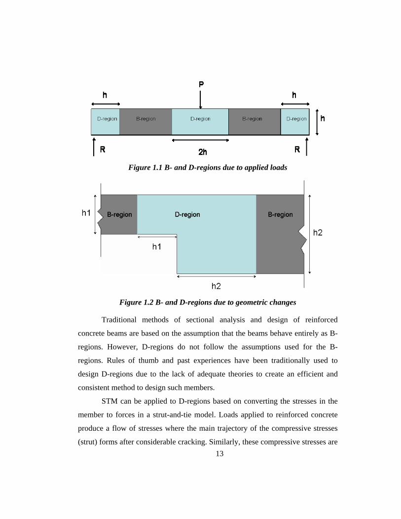
Figure 1.1 B- and D-regions due to applied loads
Figure 1.2 B- and D-regions due to geometric changes
Traditional methods of sectional analysis and design of reinforced
concrete beams are based on the assumption that the beams behave entirely as B-
regions. However, D-regions do not follow the assumptions used for the B-
regions. Rules of thumb and past experiences have been traditionally used to
design D-regions due to the lack of adequate theories to create an efficient and
consistent method to design such members.
STM can be applied to D-regions based on converting the stresses in the
member to forces in a strut-and-tie model. Loads applied to reinforced concrete
produce a flow of stresses where the main trajectory of the compressive stresses
(strut) forms after considerable cracking. Similarly, these compressive stresses are 13

14
interconnected by tensile stresses whose main trajectories can be used to identify
ties.
STM is a method based on truss models, where only axial forces are
transmitted by the struts and ties. The regions where the struts and ties intersect
each other are important elements to consider in STM. Such regions are called the
“nodal zones” or simply the nodes. Nodal zones have to be subjected to at least
three forces to satisfy equilibrium. For example, CCC represents a node resisting
three compressive forces (or struts), CTT and TTT nodes are also possible. Nodes
also have finite dimensions (length, width, height). Node geometry can be
determined by using a hydrostatic node definition where the faces of a node are
perpendicular to the axes of the struts and ties that intersect at the node. The
stresses acting on the faces of a hydrostatic node are equal.
1.2 HISTORICAL BACKGROUND
Ritter (1899) and Morsch (1902) were the first to introduce the concept of
a truss model to interpret the behavior of reinforced concrete beams (Figure 1.3).
A typical flexural member such as the one shown in Figure 1.3 is assumed to
resist the tension force acting at the bottom of the beam and is assumed to behave
like the bottom chord of a truss. The concrete compression zone at the top of the
beam is assumed to act as the top chord. Inclined compressive struts and vertically
oriented ties (stirrups) are used to model the shear transfer mechanism.

Figure 1.3 Truss model (Ritter and Mörsch)
During the 1960s, Thurliman, Marti and Mueller (Schalaich, Schäfer,
Jennewein 1987) improved this model by applying the theories of concrete
plasticity. Collins and Mitchell (1980’s) introduced the effect of deformations on
the truss model which could consider the effect of shear, torsion, bending and
axial actions. The STM design procedure was introduced in the Canadian Code
(CSA A 23.3-84) in 1984, AASHTO LRFD Bridge Design Specifications (section
5.6) in 1994 and ACI 318-02 (Appendix A) in 2002.
1.3 SCOPE OF THE PROJECT
This study focuses on examining the STM provisions of various design
codes (ACI 318-02, AASHTO LRFD Bridge Design Specifications). In order to
achieve this goal, seven specimens were tested in the Ferguson Structural
Engineering Laboratory at the University of Texas at Austin. The capacities of the
specimens were predicted using ACI 318-02 and AASTHO LRFD Bridge Design
Specifications. These predictions facilitated the comparative evaluation of ACI
318-02 and AASTHO LRFD Bridge Design Specifications.
15

CHAPTER 2 Experimental Program
2.1 INTRODUCTION
The testing program included seven shear-dominated specimens (Beams 1
- 7). These specimens were divided into two sets based on their cross-sectional
geometry (Figure 2.1). Data such as applied load, support reactions, deflections at
mid-span, strains in flexural and shear reinforcement were recorded during the
tests.
2.1 TEST SPECIMENS
The test specimens were of 14.5 feet long beams. Four of the seven
specimens had 18-in. square sections and others had 18” x 30” sections. The
amount of longitudinal reinforcement was kept constant at a reinforcement ratio
of 2% for all specimens. Figure 2.1 shows the details of the test specimens.
Figure 2.1 Test specimens
16
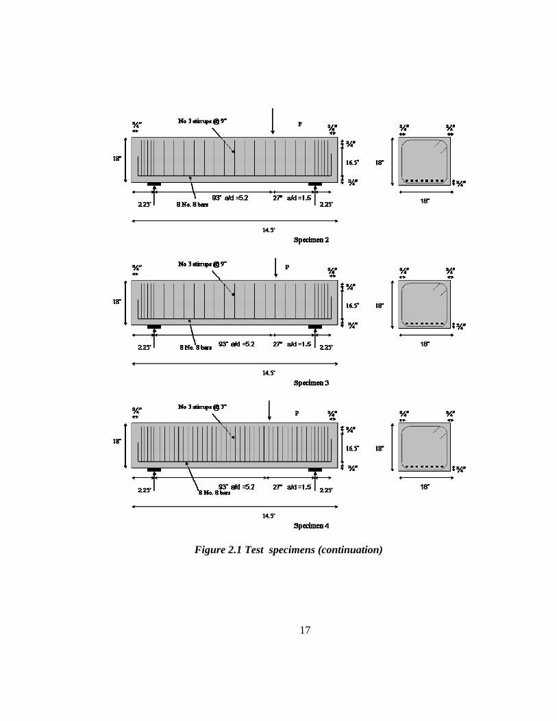
Figure 2.1 Test specimens (continuation)
17
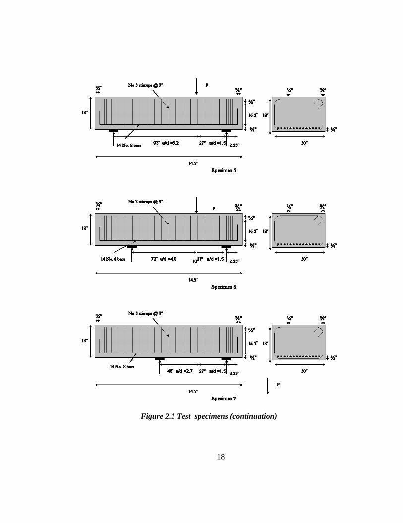
Figure 2.1 Test specimens (continuation)
18

2.2 TEST SET UP
Figure 2.2 shows the test setup used in the experimental investigation. A
double acting hydraulic ram was used to apply the loads. The capacity of the test
setup was 480 kips.
2.2.1 Frame
Figure 2.2 illustrates the test setup used in this study. The reaction frame
was made up of W-shapes.
Figure 2.2 Test Setup
19

2.2.2 Supports and their accessories
Test specimens were simply supported. One of the supports represented a
pinned support which restrained horizontal and vertical displacements and
allowed rotations. The other support was a roller that permitted horizontal
displacements and also rotations. Figure 2.3 shows the details of the supports used
in this study.
Figure 2.3 Supports
2.3 INSTRUMENTATION
2.3.1 Strain gages
Longitudinal bar strains were measured at two sections: one section at the
point of maximum moment (the section under the load point) and the other
section at one of the supports (North reaction in Figure 2.2).
In addition, stirrups were instrumented to measure the transverse strains.
Strain gauges were attached on the surface of the concrete beam to measure
compressive strains in the struts. These strain gauges were attached at varying
20

angles (30°, 45°, 60° measured from the horizontal axis) to capture the
highest/most critical compressive strain (Figure 2.4).
Figure 2.4 Strain gages on concrete
2.3.2 Potentiometers
Potentiometers were used to determine the vertical deflection of the beam
at mid span (Figure 2.5).
Figure 2.5 A typical Potentiometers
21
2.3.3 Data acquisition
Data from load cells, potentiometers, strain gauges and the loading ram
were collected using an HP scanner.
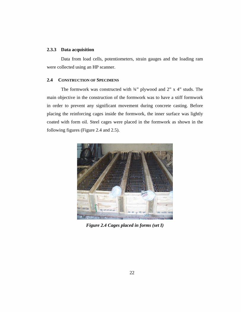
2.4 CONSTRUCTION OF SPECIMENS
The formwork was constructed with ¾” plywood and 2” x 4” studs. The
main objective in the construction of the formwork was to have a stiff formwork
in order to prevent any significant movement during concrete casting. Before
placing the reinforcing cages inside the formwork, the inner surface was lightly
coated with form oil. Steel cages were placed in the formwork as shown in the
following figures (Figure 2.4 and 2.5).
Figure 2.4 Cages placed in forms (set I)
22

Figure 2.5 Cages placed in forms (set II)
Then, concrete was poured (Figure 2.6 and Figure 2.7). Rod vibrators
were used to reduce or eliminate the formation of voids. After concrete casting
was completed the top surface of the formwork was covered with plastic (Figure
2.8).
Figure 2.6 Pouring of Concrete (set I)
23

Figure 2.7 Pouring of concrete (set II)
Figure 2.8 Plastic cover
2.5 MATERIAL STRENGTH
2.5.1 Compressive strength of concrete
All test specimens were cast at the same time in order to avoid variability
in concrete strength. 6“ x 12” standard cylinders, cast along with the test 24

specimens, were tested (Figure 2.11) to determine the compressive strength of
concrete at the time the test specimens were tested. The compressive strength of
concrete of each test specimen, determined as the average of three cylinder tests,
is given in Table 2.1.
Figure 2.9 Testing of compressive strength of concrete
Table 2.1 Geometric, reinforcement and material properties of test specimens
Bearing Plate
Dimension
Spec Test No. Section
Flexural Reinf. Shear Reinf.
South Support
North Support
f'c (psi)
fy (Ksi)
Set I
1 1 18"x18" 8 No. 8 No. 3 @ 9" 10"x18" 2-6"x7.75" 2854 73 2 2 18"x18" 9 No. 8 No. 3 @ 9" 10"x18" 6"x18" 2853 73 3 3 18"x18" 10 No. 8 No. 3 @ 9" 10"x18" 6"x15.5" 2850 73 4 4 18"x18" 11 No. 8 No. 3 @ 3" 10"x18" 6"x18" 2880 73 4 5 18"x18" 12 No. 8 No. 3 @ 3" 10"x18" 6"x15.5" 2880 73 2 6 18"x18" 13 No. 8 No. 3 @ 9" 10"x18" 6"x18" 2880 73 1 7 18"x18" 14 No. 8 No. 3 @ 9" 10"x18" 6"x18" 3130 73
Set ll 5 8 18"x30" 14 No. 8 No. 3 @ 9" 10"x18" 2-6"x7.75" 3107 73 6 9 18"x30" 14 No. 8 No. 3 @ 9" 10"x18" 2-6"x7.75" 3572 73 7 10 18"x30" 14 No. 8 No. 3 @ 9" 10"x18" 2-6"x7.75" 3646 73
25
26
2.5.1.1 Tensile strength of steel
Standard coupon tests were conducted on No. 8 bars (longitudinal steel)
and No.3 bars (transverse bars) used in the test specimens. Yield strength of the
No. 8 bars was 73 ksi.

27
CHAPTER 3 Test results
3.1 INTRODUCTION
The objective of this chapter is to describe the results from ten tests
conducted on the seven specimens. Load history, deflections, reactions at
supports, reinforcement strains, concrete strains, and test observations are
described in the following sections.
3.2 SHEAR SPANS
In order to evaluate the influence of shear span-to-depth ratio on the
behavior of test specimens, shear spans used in each test varied. Table 3.1
illustrates the shear span-to-depth ratio used in each test.
Table 3.1 Spans, North and South Shear spans
Shear spans Shear spans-to-depth ratio Span (in) North (in) South (in) North South Test 1 120 27 93 1.5 5.2 Test 2 120 27 93 1.5 5.2 Test 3 120 27 93 1.5 5.2 Test 4 120 27 93 1.5 5.2 Test 5 100 27 73 1.5 4.1 Test 6 100 27 73 1.5 4.1 Test 7 100 27 73 1.5 4.1 Test 8 120 27 93 1.5 5.2 Test 9 99 27 72 1.5 4.00
Test 10 75 27 48 1.5 2.7

Figure 3.1 Configuration of tests (east view)
3.3 TEST OBSERVATIONS
A concentrated load (Figure 3.1) was applied to each test specimen and
was increased gradually (at 5 kips load increments) until the test specimen failed.
The fist cracks to appear on both sides of the beam (east and west sides)
were flexural and were located under the applied load. Then shear cracks were
observed in the north end of the beam where there shear stresses were greater than
those in the south end of the beam. These cracks appeared at different loads for
each test specimen as shown in Table 3.2.
28

29
Table 3.2 Load at first cracking
Flexural Cracks (Kips) Shear Cracks (Kips) East and Westside East side West side Test 1 75 90 90 Test 2 65 90 80 Test 3 55 95 70 Test 4 55 80 80 Test 5 50 80 100 Test 6 60 100 100 Test 7 90 70 90 Test 8 100 160 160 Test 9 110 170 170 Test 10 110 200 200
Flexural cracks were observed on both sides at the same applied load and
the pattern they followed were also the same on both sides. Both the length and
width of the flexural cracks increased with increasing loads. In addition the
number of flexural cracks observed also increased with progressively increasing
loads.
The initial shear cracks were observed at slightly higher load levels than
the flexural cracks. The crack patterns on both sides of the test specimens were
similar.
3.4 CRACK PATTERN AT FAILURE
In specimens 1, 2, 4, 5, 6, and 7 shear failure took place in the short shear
span (Figures 3.2, - 3.7). In test 8, 9 and 10 shear failure was observed in the long
shear span (Figures 3.8 - 3.10). Failure of the test specimen 3 was different than
all the other test specimens. Crushing of concrete adjacent to the loading plate and
subsequent buckling of the compression bars was observed in this specimen.
Figures 3.11 – 3.13 demonstrate the failure of the test specimens.
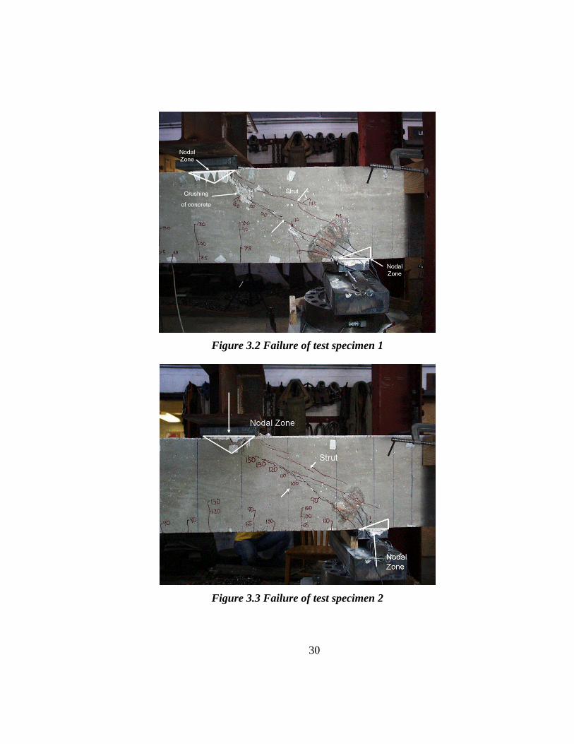
Figure 3.2 Failure of test specimen 1
Figure 3.3 Failure of test specimen 2
30

Figure 3.4 Failure of test specimen 4
Figure 3.5 Failure of test specimen 5
31

Figure 3.6 Failure of test specimen 6
Figure 3.7 Failure of test specimen 7
32

Figure 3.8 Failure of test specimen 8
Figure 3.9 Failure of test specimen 9
33
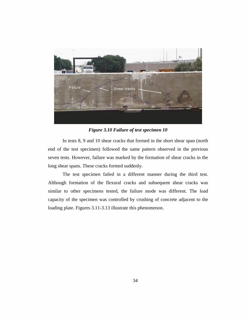
Figure 3.10 Failure of test specimen 10
In tests 8, 9 and 10 shear cracks that formed in the short shear span (north
end of the test specimen) followed the same pattern observed in the previous
seven tests. However, failure was marked by the formation of shear cracks in the
long shear spans. These cracks formed suddenly.
The test specimen failed in a different manner during the third test.
Although formation of the flexural cracks and subsequent shear cracks was
similar to other specimens tested, the failure mode was different. The load
capacity of the specimen was controlled by crushing of concrete adjacent to the
loading plate. Figures 3.11-3.13 illustrate this phenomenon.
34

Figure 3.11 Failure of test specimen 3
Figure 3.12 Picture of the failure zone after removal of lose concrete
35

Figure 3.13 Buckling of compression reinforcement
3.5 LOAD VS. MIDSPAN DEFLECTION RESPONSE
Load vs. midspan deflection response of test specimens is given in Figure
3.14. Strain gauges installed on flexural reinforcement at critical sections
(maximum moment section and at the north support) indicated that rebars did not
yield.
Load - Deflection Plot
0
50
100
150
200
250
300
350
400
0 0.1 0.2 0.3 0.4 0.5
Deflection at mid-span (in)
Loa
d (K
ips)
)
Test 1Test 2Test 3Test 4Test 5Test 6Test 7Test 8Test 9Test 10
36
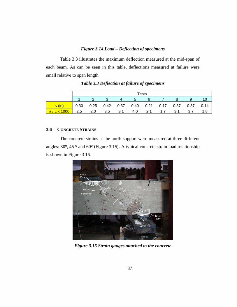
Figure 3.14 Load – Deflection of specimens
Table 3.3 illustrates the maximum deflection measured at the mid-span of
each beam. As can be seen in this table, deflections measured at failure were
small relative to span length
Table 3.3 Deflection at failure of specimens
Tests 1 2 3 4 5 6 7 8 9 10
Δ (in) 0.30 0.25 0.42 0.37 0.40 0.21 0.17 0.37 0.37 0.14 Δ / L x 1000 2.5 2.0 3.5 3.1 4.0 2.1 1.7 3.1 3.7 1.8
3.6 CONCRETE STRAINS
The concrete strains at the north support were measured at three different
angles: 30º, 45 º and 60º (Figure 3.15). A typical concrete strain load relationship
is shown in Figure 3.16.
Figure 3.15 Strain gauges attached to the concrete
37

As can be seen in Figure 3.15 the inclination of the strut that formed
between the applied load and the shape support is about 30º.
In other words the strain gauge applied at 30º degrees was essentially
parallel to the shear cracks shown in Figure 3.15.
Strain in concrete
020406080
100120140160180
-0.0009 -0.0008 -0.0007 -0.0006 -0.0005 -0.0004 -0.0003 -0.0002 -0.0001 0
Strain (in/in)
Load
(Kip
s)
30 Degrees45 Degrees60 Degrees
Figure 3.16 Concrete strain vs load relationship at the north support
In cases where the specimen failed in the short shear span (tests 1, 2, 4, 5,
6 and 7) maximum compressive strains were measured by the strain gauges that
followed the axis of the strut that formed between the load point and the north
support. Hence concrete gauges were instrumental in confirming the assumed
strut and tie models.
38
CHAPTER 4 Significance of Test Results
4.1 INTRODUCTION
In this chapter load carrying capacity of the test specimens are calculated using
Appendix A of ACI 318-02 STM provisions and chapter 5 of AASHTO LRFD Bridge
Design Specifications. These predictions are compared with the experimental values to
examine the accuracy and conservativeness of the relevant code provisions.
4.2 STRUT AND TIE MODELING PROVISIONS
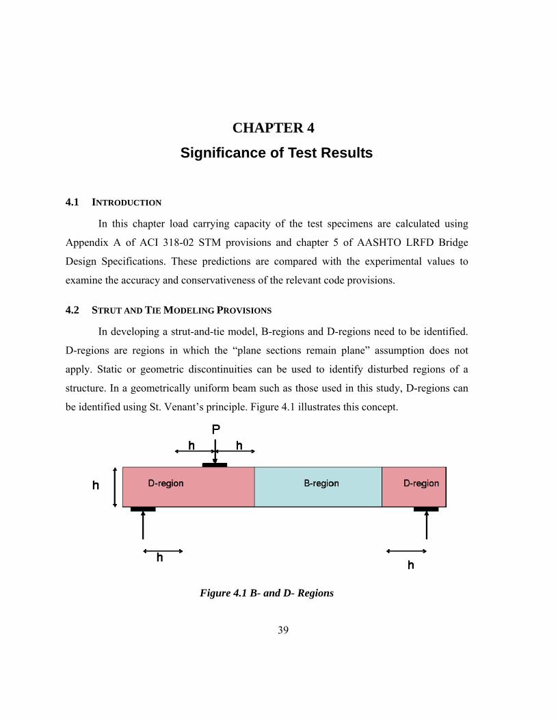
In developing a strut-and-tie model, B-regions and D-regions need to be identified.
D-regions are regions in which the “plane sections remain plane” assumption does not
apply. Static or geometric discontinuities can be used to identify disturbed regions of a
structure. In a geometrically uniform beam such as those used in this study, D-regions can
be identified using St. Venant’s principle. Figure 4.1 illustrates this concept.
Figure 4.1 B- and D- Regions
39
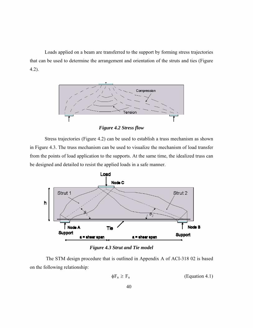
Loads applied on a beam are transferred to the support by forming stress trajectories
that can be used to determine the arrangement and orientation of the struts and ties (Figure
4.2).
Figure 4.2 Stress flow
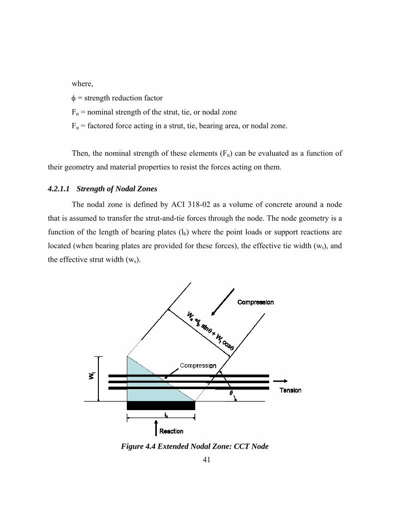
Stress trajectories (Figure 4.2) can be used to establish a truss mechanism as shown
in Figure 4.3. The truss mechanism can be used to visualize the mechanism of load transfer
from the points of load application to the supports. At the same time, the idealized truss can
be designed and detailed to resist the applied loads in a safe manner.
Figure 4.3 Strut and Tie model
The STM design procedure that is outlined in Appendix A of ACI-318 02 is based
on the following relationship:
φFn ≥ Fu (Equation 4.1)
40
where,
φ = strength reduction factor
Fn = nominal strength of the strut, tie, or nodal zone
Fu = factored force acting in a strut, tie, bearing area, or nodal zone.
Then, the nominal strength of these elements (Fn) can be evaluated as a function of
their geometry and material properties to resist the forces acting on them.
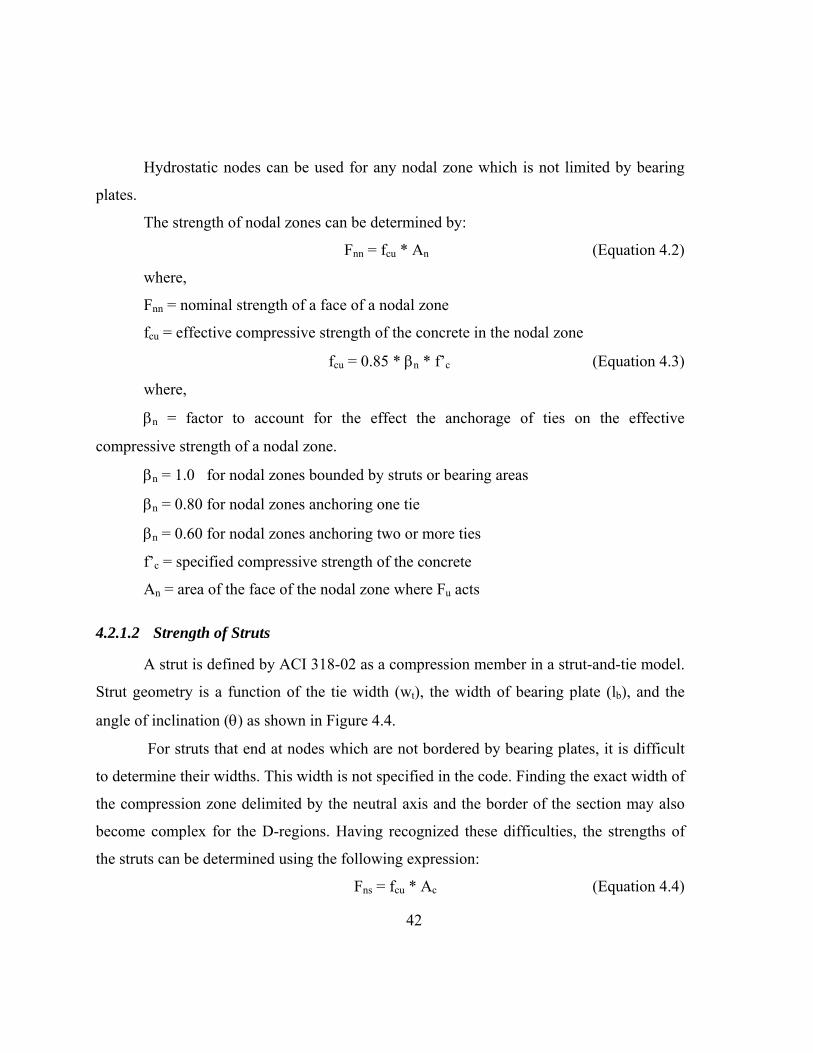
4.2.1.1 Strength of Nodal Zones
The nodal zone is defined by ACI 318-02 as a volume of concrete around a node
that is assumed to transfer the strut-and-tie forces through the node. The node geometry is a
function of the length of bearing plates (lb) where the point loads or support reactions are
located (when bearing plates are provided for these forces), the effective tie width (wt), and
the effective strut width (ws).
Figure 4.4 Extended Nodal Zone: CCT Node
41
42
Hydrostatic nodes can be used for any nodal zone which is not limited by bearing
plates.
The strength of nodal zones can be determined by:
Fnn = fcu * An (Equation 4.2)
where,
Fnn = nominal strength of a face of a nodal zone
fcu = effective compressive strength of the concrete in the nodal zone
fcu = 0.85 * βn * f’c (Equation 4.3)
where,
βn = factor to account for the effect the anchorage of ties on the effective
compressive strength of a nodal zone.
βn = 1.0 for nodal zones bounded by struts or bearing areas
βn = 0.80 for nodal zones anchoring one tie
βn = 0.60 for nodal zones anchoring two or more ties
f’c = specified compressive strength of the concrete
An = area of the face of the nodal zone where Fu acts
4.2.1.2 Strength of Struts
A strut is defined by ACI 318-02 as a compression member in a strut-and-tie model.
Strut geometry is a function of the tie width (wt), the width of bearing plate (lb), and the
angle of inclination (θ) as shown in Figure 4.4.
For struts that end at nodes which are not bordered by bearing plates, it is difficult
to determine their widths. This width is not specified in the code. Finding the exact width of
the compression zone delimited by the neutral axis and the border of the section may also
become complex for the D-regions. Having recognized these difficulties, the strengths of
the struts can be determined using the following expression:
Fns = fcu * Ac (Equation 4.4)

where,
Fns = nominal strength of a strut
fcu = effective compressive strength of a strut
fcu = 0.85 * βs * f’c (Equation 4.5)
βs = factor to account for the effect of cracking and confining reinforcement on the
effective compressive strength of the concrete in a strut:
βs = 0.75 if A.3.3 of ACI 318-02 is satisfied
βs = 0.60 if A.3.3 of ACI 318-02 is not satisfied
Where section A.3.3 of ACI can be expressed as:
003.0)γsin(**
≥∑ iisb
siA (Equation 4.6)
Asi = is the total area of reinforcement at spacing si
si = spacing of reinforcement
γi = angle between the axis of a strut and the bars in the ith layer of
reinforcement crossing that strut
b = width of beam
Ac = cross-sectional area at one end of the strut.
4.2.1.3 Strength of Ties
A tie is defined by ACI 318-02 as a tension member in a strut-tie-model. Ties are
either longitudinal or transverse reinforcement subjected to tension.
The strength of a tie is defined by:
Fnt = Ast * fy (excluding prestressed reinforcement) (Equation 4.7)
where,
Fnt = nominal strength of a tie
Ast = area of nonprestressed reinforcement in a tie
fy = specified yield strength of nonprestressed reinforcement 43

4.2.2 Calculations and Observations
In this section, capacities of the test specimens are calculated and computed
capacities are compared with the experimental values. In this way, the conservativeness of
the ACI 318-02 provisions are evaluated.
4.2.2.1 Nodal zones
Fisrt, the support reactions of the statically determinate test specimens are
calculated. Subsequently, the following three forces can be determined:
Fnn = nominal strength of node at a face of a nodal zone
Pn = nominal force of specimen at failure of node
Ptest = maximum load at failure of specimen obtained from test
Nodes A, B, and C are identified in Figure 4.5.
Figure 4.5 Nodal strengths
The strength of Node A of test specimen 1 (Figure 4.5) can be calculated as follows:
fcu = 0.85 * βn * f’c
βn = 0.8 for nodal zones anchoring one tie
94.1584.2*8.0*85.0 ==cuf ksi.
44

93"6"*5.15 ==Ac (area of bearing plate) 2in
Therefore:
5.18093*94.1Fnn == kips
(93/120) Pn = Fnn =180.5 kips (see figure 4.5)
Pn =232.9 kips
The same procedure is followed to evaluate Fnn and Pn of the other nodes (B and C)
and the nodes of the other test specimens.
4.2.2.2 Struts
The following three forces are to be determined for the struts
Fns = nominal compressive strength of a strut
Pn = external load force resulting in a strut force on Fns
Ptest = maximum load at failure of specimen obtained from a test
Struts 1 and 2 are identified in Figure 4.6
Figure 4.6 Strut strengths
The nominal strength of strut 1 of specimen 1 can be calculated as follows:
Fns= fcu * Ac
45
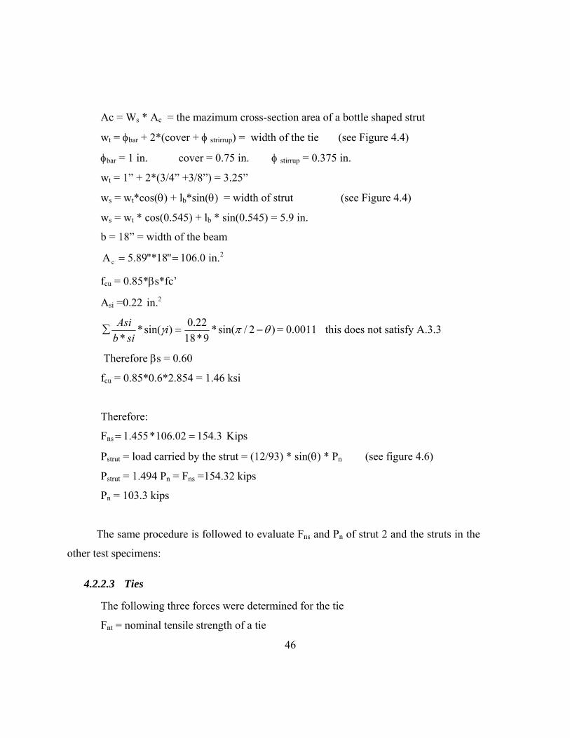
Ac = Ws * Ac = the mazimum cross-section area of a bottle shaped strut
wt = φbar + 2*(cover + φ strirrup) = width of the tie (see Figure 4.4)
φbar = 1 in. cover = 0.75 in. φ stirrup = 0.375 in.
wt = 1” + 2*(3/4” +3/8”) = 3.25”
ws = wt*cos(θ) + lb*sin(θ) = width of strut (see Figure 4.4)
ws = wt * cos(0.545) + lb * sin(0.545) = 5.9 in.
b = 18” = width of the beam
0.106"18"*89.5Ac == 2.in
fcu = 0.85*βs*fc’
Asi =0.22 2.in
)2/sin(*9*18
22.0)sin(**
θπγ −=∑ isib
Asi = 0.0011 this does not satisfy A.3.3
Therefore βs = 0.60
fcu = 0.85*0.6*2.854 = 1.46 ksi
Therefore:
Fns Kips 3.15402.106*455.1 ==
Pstrut = load carried by the strut = (12/93) * sin(θ) * Pn (see figure 4.6)
Pstrut = 1.494 Pn = Fns =154.32 kips
Pn = 103.3 kips
The same procedure is followed to evaluate Fns and Pn of strut 2 and the struts in the
other test specimens:
4.2.2.3 Ties
The following three forces were determined for the tie
Fnt = nominal tensile strength of a tie
46
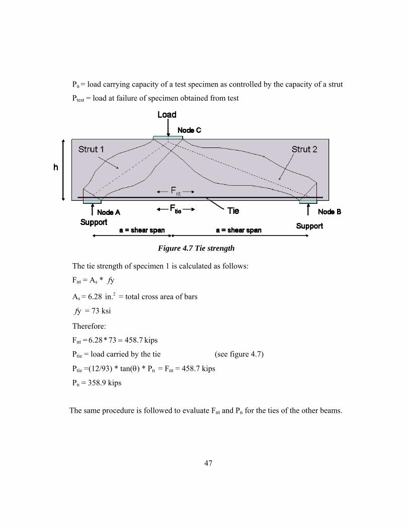
Pn = load carrying capacity of a test specimen as controlled by the capacity of a strut
Ptest = load at failure of specimen obtained from test
Figure 4.7 Tie strength
The tie strength of specimen 1 is calculated as follows:
Fnt = As * yf
As = 6.28 = total cross area of bars 2.in
yf = 73 ksi
Therefore:
Fnt = kips 7.45873*28.6 =
Ptie = load carried by the tie (see figure 4.7)
Ptie =(12/93) * tan(θ) * Pn = Fnt = 458.7 kips
Pn = 358.9 kips
The same procedure is followed to evaluate Fnt and Pn for the ties of the other beams.
47

As can be seen in Table 4.1, nodal zones or ties were not critical for the test
specimens. Accordingly, nodal zone failure was not observed during the tests. Nominal
loads (Pn) required to fail nodal zones were greater than the maximum loads applied during
the tests (Ptest), except for tests eight and nine. The high compressive strength of the nodal
zones seen in test 8 and 9 is due primarily to the tri-axial stresses developed within the node
due to confinement from the struts and bearing plates. This stress state enhances the
ultimate strength of concrete.
Table 4.1 Capacities of test specimens: ACI 318-02 predictions vs experiments
A B C Strut 1 Strut 2 Ties
Test Fnn Pn Fnn Pn Fnn Pn Fns Pn Fns Pn Fnt Pn Ptest P test / Pn
1 180.5 232.9 349.3 1552.6 436.7 436.7 154.3 103.3 129.3 99.6 458.7 358.9 130.6 1.31 2 209.5 270.4 349.2 1552.0 436.5 436.5 154.3 103.2 129.2 99.6 458.7 358.9 140.2 1.41 3 180.2 232.6 348.8 1550.4 436.1 436.1 154.1 103.1 129.1 99.5 458.7 358.9 194.9 1.96 4 211.5 272.9 352.5 1566.7 440.6 440.6 194.7 130.3 163.1 125.7 458.7 358.9 226.1 1.80 5 182.1 249.5 352.5 1305.6 440.6 440.6 194.7 138.3 177.1 143.6 458.7 381.1 246.4 1.78 6 182.1 249.5 352.5 1305.6 440.6 440.6 155.7 110.6 141.7 114.9 458.7 381.1 183.7 1.66 7 229.9 314.9 383.1 1418.9 478.9 478.9 169.2 120.2 154.0 124.8 458.7 381.1 146.2 1.22 8 196.5 253.5 633.8 2817.0 792.3 792.3 350.0 234.2 293.2 226.0 802.7 628.1 367.7 1.57 9 225.9 302.2 728.7 2671.9 910.9 910.9 402.4 286.9 368.0 299.2 802.7 669.4 343.6 1.20 10 230.6 360.3 743.8 2066.1 929.7 929.7 410.7 332.8 439.6 394.3 802.7 760.6 230.2 0.69
Table 4.1 clearly shows that strengths of the struts controlled the strength of the
beams tested in this study. As mentioned earlier, yielding of the flexural reinforcement, and
hence tie failure was not observed in any of the test conducted.
As can be seen in Table 4.1 in nine of the ten tests ACI 318-02 provisions for STM
provided safe estimates for the capacities of the beam specimens. As the ultimate strength
of the “B-region” was reached first in test 10, failure load predictions for “D-regions” in
this specimen are not meaningful. Hence, it is possible to conclude that for all specimens
that failed in the D-regions load carrying capacities were predicted safety using ACI 318-02
provisions.
48
4.3 AASHTO LRFD BRIDGE DESIGN CODE’S STRUT AND TIE MODELING PROVISIONS
STM was recently implemented in AASHTO LRFD specifications. These
specifications indicate that strut-and-tie models may be used to determine internal force
effects near supports and the points of application of concentrated loads.
AASHTO LRFD specifications recommend that STM must be used when the
distance between the center of applied loads and support reactions is less than twice the
member thickness.
Once these regions are determined, a truss configuration is created based on the
principal stress trajectories. Then, the dimensions of the struts, ties, and nodes that form this
truss can be determined. Subsequently, strength of ties, nodes and struts can be checked to
ensure safety. The strength of struts or ties can be calculated as follows:
The strength of struts or ties is based on:
Pr = φ * Pn , where:
Pr = factored axial resistance of strut or tie.
φ = resistance factor for tension or compression
Pn = nominal axial resistance of a strut or tie
4.3.1.1 Strength of Struts
The nominal resistance of an unreinforced compressive strut can be determined as follows:
Pn = fcu * Acs (Equation 4.8)
where,
Pn = nominal resistance of compressive strut
fcu = limiting compressive stress
c1
cu f'*85.0*1708.0
cf'f ≤+
=ε
(Equation 4.9)
f’c = specified compressive strength of concrete 28 days
s
2
ss1 cot*)002.0( αεεε ++= ……………… (Equation 4.10)
49
εs = tensile strain in the concrete in the direction of the tension tie
αs = the smallest angle between the compressive strut and adjoining tension ties
(deg)
Acs = effective cross-sectional area of strut
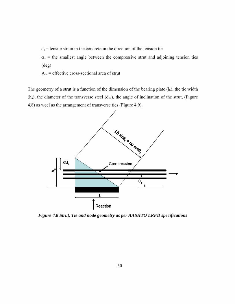
The geometry of a strut is a function of the dimension of the bearing plate (lb), the tie width
(ha), the diameter of the transverse steel (dba), the angle of inclination of the strut, (Figure
4.8) as weel as the arrangement of transverse ties (Figure 4.9).
Figure 4.8 Strut, Tie and node geometry as per AASHTO LRFD specifications
50

Figure 4.9 Strut width as per AASHTO LRFD specifications
4.3.1.2 Strength of Ties
The nominal resistance of a tension tie is:
Pn = * Ast excluding Prestressed reinforcement (Equation 4.11) yf
Pn = nominal resistance of tension tie
yf = specified minimum yield strength of reinforcing bars
Ast = area of nonprestressed reinforcement in a tie
4.3.1.3 Strength of Nodal Zones
AASHTO LRFD specifications indicate that the concrete compressive stress in the
node regions shall not exceed the concrete compressive strength of nodes. Compressive
strength of the nodes can be calculated as follows:
Compressive nodal strength = 0.85 φ f’c for nodes bounded by compressive struts
and bearing areas
51

52
Compressive nodal strength = 0.75 φ f’c for nodes anchoring one tension tie
Compressive nodal strength = 0.65 φ f’c for nodes anchoring more than one
tension tie
where,
f’c = specified compressive strength of concrete at 28 days
φ = resistance factor for tension or compression
4.3.2 Calculations and Observations
Designers usually choose εs as the yield strain (εy) in Equation 4.10.
Accordingly εs = 0.00207 is used to calculate ε1 in Equation 10 for concrete capacity
bars. In addition the strain readings obtained from the strain gages on the reinforcing
bars during testing (εtest) will also be used to determine the effect of using εs =εy in
design.
AAHSTO LRFD indicates that εs varies over the width of a strut-and-that it
is appropriate to use the value at the center line of the strut. Therefore, the values of
the afore mentioned strains (εy and εtest ) at the centerline of the strut will also be
considered for the following calculations.
4.3.2.1 Nodal zones
The following three forces were determined for the nodal zones:
Fnn = nominal strength of node at a face of a nodal zone
Pn allowable = nominal force of specimen at failure of nodal zone
Ptest = load at failure of specimen registered from test
An example of calculation of strength of nodal zone A of Test 1 (Figure 4.5) is
shown next:
Concrete compressive stress capacity = 0.75 * f’c for nodes anchoring a tension tie.
Ac = area limited by the bearing plates = 93"6"*5.15 = 2in
Fnn = Ac*0.75 * f’c
Fnn = 93*0.75*2.854 = 199.1 kips
(93/120) Pn allowable = Fnn = 199.1 kips
Pn allowable = 256.9 kips (see Figure 4.5)
The same procedure is followed to evaluate Fnn and Pn allowable of the other nodes (B
and C) as well as the nodes of the other test specimens.
4.3.2.2 Struts
The following three forces were determined for the struts
Pn = nominal strength of a strut
Pn allowable = nominal force of specimen at failure of strut
Ptest = maximum load at failure of specimen obtained from test
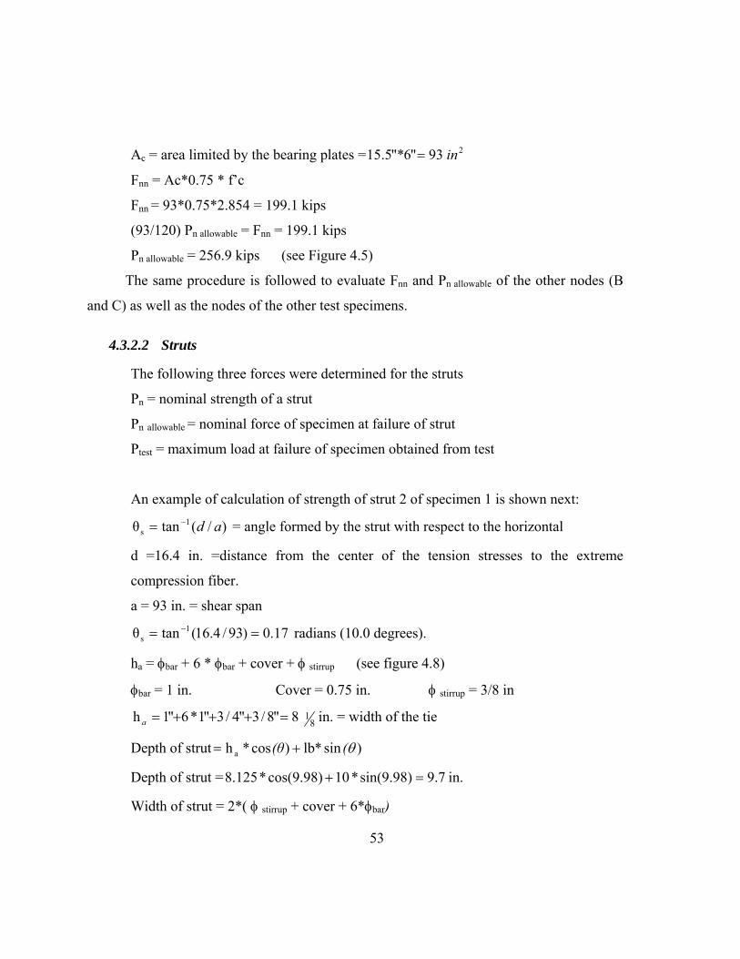
An example of calculation of strength of strut 2 of specimen 1 is shown next:
)/(tanθ 1s ad−= = angle formed by the strut with respect to the horizontal
d =16.4 in. =distance from the center of the tension stresses to the extreme
compression fiber.
a = 93 in. = shear span
17.0)93/4.16(tanθ 1s == − radians (10.0 degrees).
ha = φbar + 6 * φbar + cover + φ stirrup (see figure 4.8)
φbar = 1 in. Cover = 0.75 in. φ stirrup = 3/8 in
8"8/3"4/3"1*6"1h =+++=a 81 in. = width of the tie
Depth of strut )sinlb)cos*h a θ(*(θ +=
Depth of strut = 7.9sin(9.98)*10cos(9.98)*8.125 =+ in.
Width of strut = 2*( φ stirrup + cover + 6*φbar)
53

width of strut = 2 * (3/4” + 3/8” + 6*1) = 14.25 in.
Effective cross section area of strut = 14.25” * 9.73” = 138.73 in2.
εs = 0.001259 in/in = yielding strain of tie at center line of node
ε1 )0.10(cot*)002.00013.0(0013.0 2++=
ε1 = 0.1063 in/in
fcu 11.0*1708.02.85
+=
fcu = 0.15 ksi
Pn = Effective area * fcu = 21.0 Kips
Pstrut = load carried by the strut = (12/93) * sin(θ) * Pn allowable
Pstrut = 1.494 Pn allowable = Pn = 21.0 kips (see figure 4.6)
Pn allowable = 16.2 kips
The same procedure is followed to evaluate Pn and Pn allowable of strut 2 and the other
struts of the other beams.
4.3.2.3 Ties
The following three forces were determined for the tie
Pn = nominal resistance of tension tie
Pn allowable = nominal force at failure of beam as a function of tie strength
Ptest = load at failure of specimen obtained from test acting on a tie.
An example of calculation of the strength of the tie is shown next:
Pn fy As = 6.28 fy = 73 ksi *As= 2.in
Pn Kips 7.45873*28.6 ==
Ptie = load carried by the tie = =(12/93) * tan(θ) * Pn allowable
1.278 Pn allowable = Pn = 458.7 kips
54

55
Pn allowable = 358.9 kips
The same procedure is followed to evaluate Pn and Pn allowable for the ties of the other
beams.
Table 4.2 Summary of strengths of every element of every test (kips)
Node A Node B Node C Strut 1 Strut 2 Tie
Test Fnn Pn
allowable Fnn Pn
allowable Fnn Pn
allowable Pn Pn
allowable Pn Pn
allowable Pn P
allowable Ptest 1 199.1 256.9 385.3 1712.4 436.7 436.7 162.3 108.6 21.0 16.2 458.7 358.9 130.62 231.1 298.2 385.2 1711.8 436.5 436.5 162.3 108.6 21.0 16.2 458.7 358.9 140.23 198.8 256.5 384.8 1710.0 436.1 436.1 162.1 108.5 20.9 16.1 458.7 358.9 194.94 233.3 301.0 388.8 1728.0 440.6 440.6 163.8 109.6 21.2 16.3 458.7 358.9 226.15 200.9 275.2 388.8 1851.4 440.6 440.6 163.8 116.4 34.5 28.0 458.7 381.1 246.46 200.9 275.2 388.8 1440.0 440.6 440.6 163.8 116.4 34.5 28.0 458.7 381.1 183.77 253.5 347.3 422.6 1565.0 478.9 478.9 178.0 126.5 37.5 30.4 458.7 381.1 246.48 216.7 279.6 699.1 3107.0 792.3 792.3 176.7 118.2 22.8 17.6 802.7 628.1 367.79 249.1 342.6 482.2 1768.1 546.5 546.5 203.2 144.9 44.0 35.8 802.7 669.4 343.610 254.3 397.4 492.2 1367.3 557.8 557.8 203.2 144.9 98.2 88.1 802.7 760.6 230.2
Nodal zone failure was not observed in any of the tests, which is consistent with the
high capacities of the nodes (Fnn) (Table 4.2). Except for tests eight and nine were Pn, allowable
was smaller than Ptest.
In these tests (8 and 9) nodal zone A was the most critical node with bearing plates
that did not cover the entire area of the bottom of the beam. These bearing plates were used
to support the forces at the assumed struts developed at the sides of a beam section as per
AASHTO provisions (see Figure 4.9). Therefore, the area of the bearing plates was small
enough to only support a nominal force (Pn allowable) that was lower than the failure load
(Ptest).
Not having failures in nodal zone A as predicted by AASTHO inn tests 8 and 9
indicates that either the compressive strength of the concrete at that region is enhanced by
the confinement provided by the bearing plates or the struts are developed in an area
56
beyond the limits established by six times the diameter of the longitudinal reinforcement
(Figure 4.9).
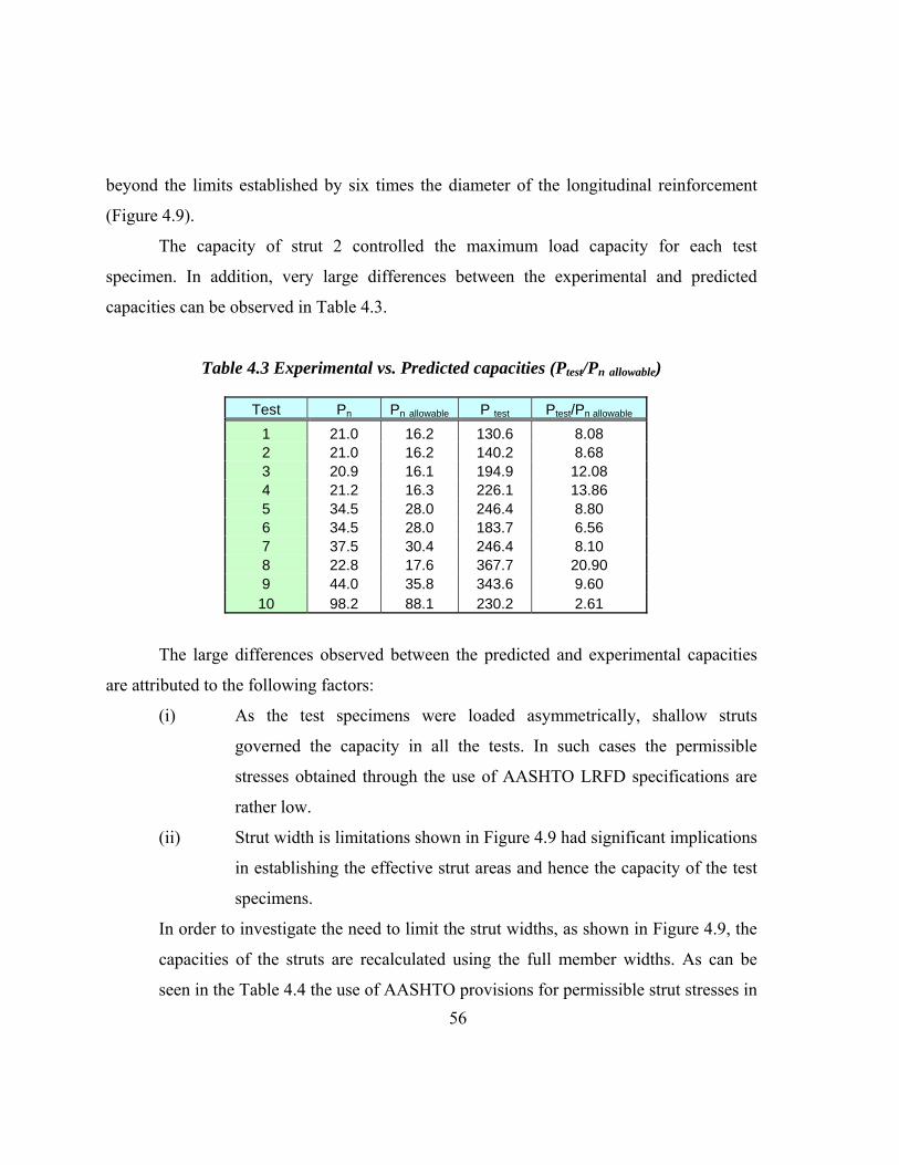
The capacity of strut 2 controlled the maximum load capacity for each test
specimen. In addition, very large differences between the experimental and predicted
capacities can be observed in Table 4.3.
Table 4.3 Experimental vs. Predicted capacities (Ptest/Pn allowable)
Test Pn Pn allowable P test Ptest/Pn allowable 1 21.0 16.2 130.6 8.08 2 21.0 16.2 140.2 8.68 3 20.9 16.1 194.9 12.08 4 21.2 16.3 226.1 13.86 5 34.5 28.0 246.4 8.80 6 34.5 28.0 183.7 6.56 7 37.5 30.4 246.4 8.10 8 22.8 17.6 367.7 20.90 9 44.0 35.8 343.6 9.60 10 98.2 88.1 230.2 2.61
The large differences observed between the predicted and experimental capacities
are attributed to the following factors:
(i) As the test specimens were loaded asymmetrically, shallow struts
governed the capacity in all the tests. In such cases the permissible
stresses obtained through the use of AASHTO LRFD specifications are
rather low.
(ii) Strut width is limitations shown in Figure 4.9 had significant implications
in establishing the effective strut areas and hence the capacity of the test
specimens.
In order to investigate the need to limit the strut widths, as shown in Figure 4.9, the
capacities of the struts are recalculated using the full member widths. As can be
seen in the Table 4.4 the use of AASHTO provisions for permissible strut stresses in

57
conjunction with full member width provide safe estimates for the member
capacities and reduce the unnecessary levels of conservatism.
Table 4.4 The influence of strut width on member capacities (kips)
Pn (AAHSTO)
Pn (AAHSTO)
Pn (width of beam) P test
P test / Pn all width
8 17.59 37.04 367.69 9.93 9 35.80 75.37 343.60 4.56 10 88.12 185.51 230.22 1.24
In order to investigate the impact of using yield strain in obtaining the permissible
strut stresses, experimentally evaluated strains are used in capacity estimates. These
estimates are then compared with the conventional calculations where steel strain is taken
as yield strain. As can be seen in Table 4.5 the use of εy (rather than the strain measured
during the tests) reduces the nominal capacities by about 20%. This certainly adds to the
excessive conservatism of the AASHTO LRFD specifications for STM.
Table 4.5 Nominal loads at εy and εtest
Pn allowable
Test Pn εy
(kips) Pn εtest (kips)
P test (kips) Pn(εy) /Pn (εtest)
1 16.2 20.2 130.6 0.801 2 16.2 20.2 140.2 0.801 3 16.2 20.1 194.9 0.801 4 16.3 20.3 226.1 0.801 9 43.4 53.9 343.6 0.804 10 141.0 173.4 230.2 0.813
If reinforcing bars strains at the centerline of the compressive struts are used in
capacity estimations, the nominal capacities of the struts (and hence the beams) increase by
about 35-40% (Table 4.6). Hence it is clear that selection o the strain has important
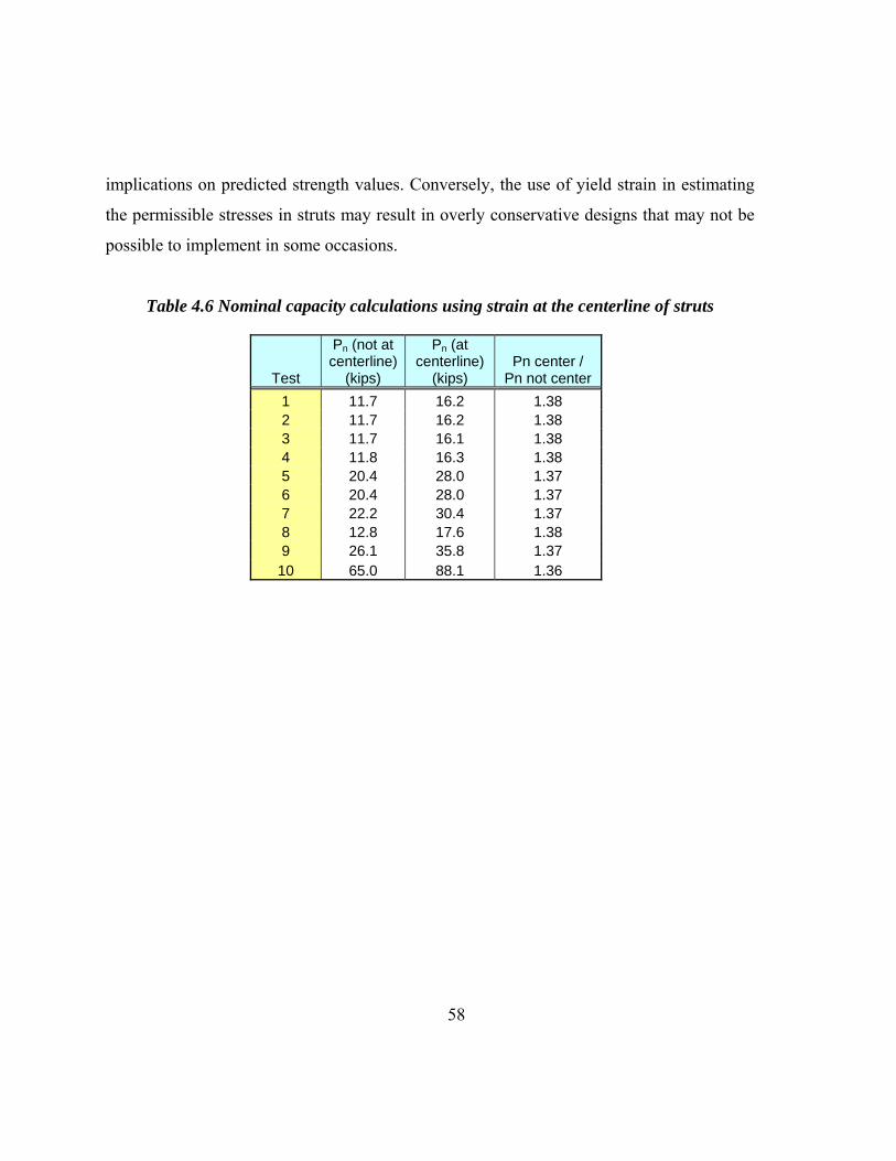
58
implications on predicted strength values. Conversely, the use of yield strain in estimating
the permissible stresses in struts may result in overly conservative designs that may not be
possible to implement in some occasions.
Table 4.6 Nominal capacity calculations using strain at the centerline of struts
Test
Pn (not at centerline)
(kips)
Pn (at centerline)
(kips) Pn center /
Pn not center 1 11.7 16.2 1.38 2 11.7 16.2 1.38 3 11.7 16.1 1.38 4 11.8 16.3 1.38 5 20.4 28.0 1.37 6 20.4 28.0 1.37 7 22.2 30.4 1.37 8 12.8 17.6 1.38 9 26.1 35.8 1.37 10 65.0 88.1 1.36
59
CHAPTER 5 Conclusions
The following conclusions can be reached based on this research study:
• Strut-and-tie modeling is a powerful technique that can be used to design
D-regions of structural members.
• Both AASHTO LRFD Bridge Design Specifications and ACI 318-02
provide safe estimates for the load carrying capacities of the test
specimens
• AASHTO LRFD Bridge Design Specifications provide overly
conservative strength predictions. This is primarily due to the restrictive
nature of the AASHTO Specification’s provisions for strut widths and
permissible stresses for shallow strut angles.
• Based on the ten tests conducted on seven beams, it can be concluded that
full widths of the members can be used to calculate strut capacities.
• The use of yield strain in establishing the permissible strut stresses
(AASHTO LRFD Bridge Design specifications) appears to be a safe
assumption. However, for the specimens tested in this study such a safe
estimation of the reinforcing bar strain at the centerline of a strut resulted
in excessive levels of conservatism.
REFERENCES
1. ACI 318 2002: Building Code Requirements for Structural Concrete Code and
Commentary, American Concrete Institute, Farmington Hills, MI.
2. AAHSTO LRFD Bridge Design Specifications, American Association of State Highway Transportation Officials, 444 North Capitol Street, N. W. Suite 249, Washington, D.C., 2001, ISBN: 1-56061-194-3, Second Edition, 1998.
3. Schalaich, Schäfer, Jennewein 1987: J. Schalaich, K Schäfer, M. Jennewein, Toward a Consistent Design of Structural Concrete, PCI Journal, Prestressed Concrete Institute, Vol. 32, No. 3, May-June 1987, pp. 74-150.
4. Hagenberger, Breen 2002: B. Chen, M. Hagenberger, J. E. Breen, Evaluation of Strut-and-Tie Modeling Applied to Dapped Beam with Opening, ACI Structural Journal Julay-August 2002, Technical Paper Tile no. 99-S46,
5. Marti 1985: P. Marti, Basic Tools of Reinforced Concrete Beam Design, ACI Journal January-February 1985, Technical Paper Title no. 82-4.
60