Embed Size (px)
Citation preview

i
Copyright by: Benjamin James Warren (2015)
ii
FIELD APPLICATION OF EXPANDING RIGID POLYURETHANE STABILIZATION OF
RAILWAY TRACK SUBSTRUCTURE
by
BENJAMIN JAMES WARREN
A thesis submitted in partial fulfillment
of the requirements for the degree of
MASTER OF SCIENCE
CIVIL AND ENVIRONMENTAL ENGINEERING
at the
UNIVERSITY OF WISCONSIN-MADISON
Spring 2015
iii
FIELD APPLICATION OF EXPANDING RIGID POLYURETHANE STABILIZATION OF
RAILWAY TRACK SUBSTRUCTURE
____________________ ____________________
Students Name campus ID number
Approved:
_____________________________ _____________________________
signature date signature date
James M. Tinjum, Associate Professor Tuncer B. Edil, Professor Emeritus

iv
Dedication
To Mom, Dad, Andy, and Chris for unconditional love and support.

v
Executive Summary
This project includes the use of expanding rigid polyurethane foam to remediate substructure
deficiencies in railroad track at a field site in Illinois. Soft substructure soils exhibit creep or
consolidation that lead to excess track settlement. Cyclic loading from passing trains can fail the
subgrade, with progressive cyclic shear failure. Track settlement and progressive shear failure
were found at a field sites in Dayton, Illinois. Following a geotechnical and geophysical
investigation of the sites, URETEK USA planned a polyurethane injection strategy to compress
the subgrade soils and permeate the subballast layer. Polyurethane injection was compared to
traditional railroad maintenance with a Life-Cycle Cost Analysis and Life-Cycle Analysis. Due to
weather and scheduling difficulties, the injection results will be appended and included in a final,
updated report.
A full-scale prototype model is often the ideal simulation of the final product for field application.
Therefore, in geotechnical engineering, different models are developed to test proposed
construction methods, interaction between elements, and field performance. Areas where
experimental products are used in full-scale applications, and that are constructed with traditional
equipment and techniques, are invaluable to researchers and industry alike. The prototyped
product can be evaluated in real-world conditions, where not all variables can be closely
controlled. Laboratory tests, while important, cannot replicate porewater distributions and soil
heterogeneity in the environment where the product is proposed for use.
The expanding rigid polyurethane enhanced ballast research began in 2011 with Keene (2012)
investigating the performance of clean ballast injected with polyurethane (PUR) in a collaboration
of with UW-Madison and URETEK USA. PUR strengthened the ballast layer in both compression
and flexural tests. Dolcek (2013) investigated the same PUR, but with injection into ballast with
varying amounts of fouling (fine) materials and water content. Similar to Keene (2012), the
mechanical behavior was enhanced in both compression and flexural, but flexural performance

vi
of fouled ballast was below that of the clean ballast. Enhancement of the ballast layer was proven
over repeated experiments with different ballast types and gradations and resulted in the
motivation to test this technology in the field.
A railroad track site was chosen in Dayton, Illinois, for which fraccing sand is transported to test
the performance of a substructure deficient section of railroad injected with PUR. This spur line
receives fully loaded unit trains on a near daily basis. Car switching and train assembly (putting
cars in proper positions for transportation) occurs here as well. The track borders the Fox River,
and there are substructure problems with: soft soil, settlement, and embankment failures along
this stretch of track.
To clarify what the contributing underlying problems are at the track field site, the “Dayton Dip,”
geotechnical and geophysical investigations were conducted. URETEK USA/ICR provided
Dynamic Cone Penetrometer logs, which give an indication of soil strength. The UW-Madison
team conducted Ground Penetrating Radar, Electrical Resistivity Tomography, Time Domain
Reflectometry, and excavated test pits to take samples to run engineering property tests in a
laboratory setting. The data from these different tests collectively verified the hypothesis of a
highly fouled ballast layer, with a soft saturated clay subgrade beneath. There were classic
subgrade shear failures along the track and at bridge approaches; i.e., the “bump at the end of
the bridge” in which an abrupt change in track stiffness causes differential settlement.
The investigation assisted in the design of two types of polyurethane injection: one to strengthen
the subballast and one to strengthen and stiffen soft subsurface material. With URETEK USA’s
background in polyurethane injection for infrastructure projects, including rail crossings, their
expertise was necessary in designing a functional and economical injection package. The
injection was proposed as a combination of subballast layer strengthening and URETEK Deep
Injection (UDI) to strengthen and stiffen the subgrade. Due to imposed restrictions of the railroad,
PUR could not be placed within 30 cm of the bottom of the tie.
vii
The evaluation of polyurethane injection included mobilization and construction costs, track
stiffening, maintenance, and environmental impact. Fast construction time decreases user costs
and inconveniences. Furthermore, environmental impact has become an important consideration
in construction projects. Polyurethane injection can fulfill these metrics. A life-cycle cost analysis
was conducted with inputs from URETEK and Wisconsin and Southern Railroad, over a ten-year
period. Over a 10-year period, PUR injection appears to be a superior improvement methodology
to traditional maintenance resulting in a cost savings from $1000 - $20,000 depending on discount
rate. In the life-cycle analysis, PUR injection results in use of water, and CO2 emissions, 82%,
and 5% respectively, compared to traditional maintenance methods.
After the ongoing portion of this project are completed, various instruments and techniques will
be used to monitor the rail section. To measure the dynamic properties and track modulus, strain
gauges will be used to measure the cumulative strain in the super-structure and sub-structure of
the track. Survey reflectors will be installed every 2 m on both sides of the rail to measure
settlement and differential settlement between rails. Finally, settlement rods will be installed to
isolate the response of different layers and their corresponding contribution to the permanent
deformation in the railroad track. An un-injected control section will be also instrumented to
compare results and assess PUR effectiveness. Due to schedule constraints (e.g., early onset
of cold weather in 2014), the injections were not completed before the completion of this thesis.
Therefore, when the pilot study is completed and analyzed, results will be appended, and a final,
updated report issued to the project sponsors.
Included in the Appendix are laboratory tests of environmental impacts on polyurethane stabilized
fouled ballast and rigid polyurethane foam. Freeze-thaw cycling was conducted; degradation was
tracked and tested with non-destructive methods and cyclic triaxial testing. No effect was
determined after 20-freeze-thaw cycles. Long term water absorbance of polyurethane foam was
investigated. Samples were submerged for 120-days then tested in unconfined compression.

viii
Minimal, approximately 3%, changes were seen from ideal polyurethane samples. The results
from freeze-thaw cycling and water absorbance indicate that PUR will remain stable in field
conditions.

ix
Acknowledgements
I owe my success at the University of Wisconsin Madison to many individuals. Professors Edil,
Fratta, and Tinjum for their guidance and support during my undergraduate and graduate studies.
Andrew Keene for pioneering this research and involving me in the world of railroads and
polyurethane; without him, my path through graduate school would not have been possible.
Xiaodong (Buff) Wang for all the insight on laboratory testing, instrumentation, field work methods
and fishing. Abdullah Alsabhan for the help whenever I needed it, whether it be field work or
complex problems.
This study was made possible by funding from the Center for Freight Infrastructure Research and
Education (CFIRE). URETEK ICR and URETEK USA provided support in field investigation
efforts and polyurethane injection strategies. Special thanks is given to Dr. Randy Brown, Jack
Frey, Rex Klentzman, and Steve Reed.
During my graduate study, various graduate/undergraduate students and friends in the Civil and
Environmental Engineering Department at the University of Wisconsin-Madison have kept me
sane and improved my personal and professional life; they include Damien Hesse, Junwei Su,
Matt Walker, Faith Zangl, Tolga Dolcek, Erin Hunter, Ali Soleimanbeigi, Brigitte Brown, Hua Yu,
David Wang, Paulo Florio, and many others.

x
Table of Contents Dedication ................................................................................................................................ iv
Executive Summary .................................................................................................................. v
Acknowledgements ................................................................................................................. ix
List of Figures ......................................................................................................................... xii
List of Tables .......................................................................................................................... xiv
Chapter 1 .................................................................................................................................. 1
Thesis Outline ....................................................................................................................... 1
Track Background ................................................................................................................ 3
Track Design & Maintenance ............................................................................................... 7
Ballast Layer Determination ................................................................................................ 7
HMA Underlayment .............................................................................................................12
Maintenance Methods .........................................................................................................13
Geosynthetic use in Rail Applications ...............................................................................16
Polyurethane (URETEK 486) ...............................................................................................18
Polyurethane in Rail ............................................................................................................19
URETEK Injection System ..................................................................................................22
Chapter 2: Decision Making ...................................................................................................24
Life Cycle Cost Analysis Background ...............................................................................24
Life Cycle Analysis Background ........................................................................................28
Monte Carlo Simulation.......................................................................................................32
Chapter 3: Geotechnical Field Investigation .........................................................................33
Geotechnical and Geophysical Investigation Overview ...................................................33
Ballast Site ...........................................................................................................................38
Concrete Site .......................................................................................................................43
Culvert Site ..........................................................................................................................47
Bridge Approach - Summary Report ..................................................................................51
Laboratory Analyses ...........................................................................................................65
Discussion of Field Results ................................................................................................70
Geotechnical Field Methods ...............................................................................................76
Laboratory Results ..............................................................................................................79
Chapter 4: LCCA and LCA Outcomes ....................................................................................83
LCCA Inputs and Results ....................................................................................................83
LCA Inputs and Results ......................................................................................................89
Monte Carlo Simulation.......................................................................................................99

xi
Chapter 5: Field Injection Design and Instrumentation ...................................................... 110
Injection Strategy .............................................................................................................. 110
Instrumentation ................................................................................................................. 116
Chapter 6 ............................................................................................................................... 118
Concluding Remarks ......................................................................................................... 118
Chapter 7: References .......................................................................................................... 119
Appendix A ............................................................................................................................ 125
Freeze-Thaw Cycling ......................................................................................................... 125
PUR Water Absorbance .................................................................................................... 135
Stress Strain Behavior of Polyurethane Foam ................................................................ 140
Further Explanation of Methods ....................................................................................... 142
Appendix B ............................................................................................................................ 147
Selected Figures ................................................................................................................ 147
Appendix C: Proposed instrumentation .............................................................................. 151
Rail reflectors .................................................................................................................... 151
Settlement gauges ............................................................................................................. 151
Strain gauges ..................................................................................................................... 152

xii
List of Figures
Figure 1: Railroad cross section ................................................................................................. 3 Figure 2: Stress Distribution (Selig and Waters, 1994) ............................................................... 8 Figure 3: URETEK Injection System (www.uretek.com) ............................................................22 Figure 4: Typical LCCA Process (Hsu, 2011) ............................................................................24 Figure 5: Typical LCA Construction modified from (wrtassoc.com) ............................................28 Figure 6: Ballast site track condition ..........................................................................................33 Figure 7: GPR survey technique ...............................................................................................35 Figure 8: Geological resistivity ranges (www.eos.ubc.ca) ..........................................................36 Figure 9: Google Earth image of site locations ..........................................................................37 Figure 10: Total station survey data for Ballast site ...................................................................38 Figure 11: Ballast site overview .................................................................................................39 Figure 12: DCP results for Ballast site .......................................................................................40 Figure 13: GPR survey line .......................................................................................................41 Figure 14: GPR result with DCP overlay ...................................................................................41 Figure 15: ER section for Ballast site ........................................................................................42 Figure 16: Concrete site view. Note ditch location. V-blocks are highlighted by red arrow. ........43 Figure 17: DCP results for track test ........................................................................................45 Figure 18: DCP results for ditch ................................................................................................45 Figure 19: Vertically corrected DCP results ...............................................................................45 Figure 20: ERT section for Concrete site ...................................................................................46 Figure 21: View of the culvert section. .......................................................................................47 Figure 22: DCP results for Culvert site ......................................................................................48 Figure 23: GPR survey line .......................................................................................................49 Figure 24: GPR result with DCP overlay ...................................................................................49 Figure 25: ERT section for Culvert site ......................................................................................50 Figure 26: View of bridge facing north .......................................................................................51 Figure 27: Site layout from Google Earth ..................................................................................52 Figure 28: Mile Marker 75. Note: Ballast and shoulder washout with support structure .............53 Figure 29: TDR waveform with multiple reflections at the DCP location ....................................54 Figure 30: GPR survey direction ...............................................................................................55 Figure 31: GPR profile with DCP overlay at the center line survey of the two bridge approaches
.................................................................................................................................................56 Figure 32: GPR profile with DCP overlay at the east shoulder survey of the two bridge
approaches ...............................................................................................................................57 Figure 33: GPR survey direction ...............................................................................................57 Figure 34: GPR profile with DCP overlay at the west shoulder survey of the two bridge
approaches ...............................................................................................................................58 Figure 35: ERT results from North Section ................................................................................59 Figure 36: ERT Results from the South Section ........................................................................60 Figure 37: Test pit pictures from different angles. Picture on the left has rough delineation of soil
layers ........................................................................................................................................61 Figure 38: Depths and thicknesses of soil layers .......................................................................62 Figure 39: From left to right: ballast, subballast, coal material, and subgrade ...........................62 Figure 40: DCP test results .......................................................................................................63

xiii
Figure 41: Grain size distributions .............................................................................................66 Figure 42: Cyclic triaxial ballast test results ...............................................................................67 Figure 43: Subgrade grain size distribution ...............................................................................68 Figure 44: Subgrade consolidation curves ................................................................................69 Figure 45: Failure Mechanisms by Li and Selig, 1998 and Hay (1981) ......................................70 Figure 46: Subgrade failure .......................................................................................................71 Figure 47: South Approach .......................................................................................................73 Figure 48: GPR and DCP result comparison .............................................................................78 Figure 49: Cyclic triaxial ballast test results ...............................................................................81 Figure 50: Maintenance Variable Effect ....................................................................................85 Figure 51: LCA quantity comparison .........................................................................................92 Figure 52: Normalized comparison of PUR injection compared to traditional maintenance
methods ....................................................................................................................................93 Figure 53: Normalized contributions for PUR injection ..............................................................94 Figure 54: Normalized contributions for traditional maintenance ...............................................95 Figure 55: Net resource usage for PUR injection ......................................................................97 Figure 56: PDF for kg CO2 eq. for traditional maintenance ..................................................... 104 Figure 57: PDF for Water depletion for traditional maintenance .............................................. 105 Figure 58: PDF for kg Oil for traditional maintenance .............................................................. 106 Figure 59: PDF for kg CO2 eq. for PUR injection .................................................................... 107 Figure 60: PDF for water depletion for PUR injection .............................................................. 108 Figure 61: PDF for kg Oil for PUR injection ............................................................................. 109 Figure 62: Compaction grouting (skanska.co.uk) .................................................................... 113 Figure 63: Injection plan for ballast section ............................................................................. 114 Figure 64: Injection plan for bridge approach .......................................................................... 115 Figure 65: Freeze and thaw timing .......................................................................................... 128 Figure 66: Freeze Thaw Weight Tracking ................................................................................ 129 Figure 67: F-T Height Tracking ............................................................................................... 130 Figure 68: F-T Circumference Tracking ................................................................................... 130 Figure 69: Constrained modulus regression ............................................................................ 132 Figure 70: Constrained modulus tracking ................................................................................ 132 Figure 71: Cyclic triaxial results for F-T specimens ................................................................. 134 Figure 72: Cellular foam density and strength (Szycher, 1999) ............................................... 135 Figure 73: PUR strength of absorbed and dry specimens ....................................................... 138 Figure 74: Stress-strain behavior of cellular foams (Ashby, 1983) ........................................... 140 Figure 75: Inputs for 1 kg of Polyurethane in SimaPro ............................................................ 147 Figure 76: Inputs for 1000 kg of ballast in SimaPro ................................................................. 148 Figure 77: Monte Carlo simulation for PUR injection ............................................................... 149 Figure 78: LCCA calculation for ballast at 10% discount rate .................................................. 150 Figure 79: RSAK130 target ..................................................................................................... 151 Figure 80: Modified borros-type anchor: Grainger part no. 4LVK6........................................... 152

xiv
List of Tables
Table 1: Summary table for ballast condition .............................................................................66 Table 2: Ballast properties ........................................................................................................67 Table 3: Subgrade engineering properties ................................................................................68 Table 4: Coefficients of compression, reloading, and preconsolidation stress ...........................82 Table 5: General maintenance costs .........................................................................................83 Table 6: NPV results with different discount rates .....................................................................86 Table 7: Average category quantities for LCA ...........................................................................92 Table 8: Contributions for processes in LCA .............................................................................92 Table 9: Monte Carlo Results .................................................................................................. 101 Table 10: Water absorbance ................................................................................................... 137

1
Chapter 1
Thesis Outline
This thesis is presented in five chapters, each outlining a specific process in the background,
development, construction and/or injection of PUR grout intended for railroad substructure.
Chapter 1 provides a background of rail infrastructure and construction. The components are
explained as well as the design methods to determine aggregate layer thicknesses. Alternative
track design and basic maintenance methods are also included. The rigid polyurethane foam has
properties ranging between a geosynthetic and a geofoam. Geosynthetic uses in railroad
applications are covered. Geofoam use and manufacturing is included as well, thus demonstrating
that rigid cellular PUR is a similar product. Finally, an overview of the URETEK PUR material and
injection process is provided as well as additional uses of PUR in railroads.
Chapter 2 is a short chapter that functions as an introduction to Life Cycle Cost Analysis (LCCA)
and Life Cycle Analysis (LCA). With these tools it is possible to determine the optimum product in
economy and resource usage over a period of time. The cost of the soil injections (LCCA) and
the impact of the soils injections (LCA) are compared against traditional railroad maintenance.
Chapter 3 includes a report on the geophysical and geotechnical investigation of the proposed
field sites. The investigation was conducted in two parts: September 2014 and April 2015.
September 2014 included tangent track constructed over cut and fill areas. April 2015 was for
tangent track, but was focused on settlement at bridge approaches. The methods, results, and a
discussion is provided. A brief explanation, results, and discussion from the laboratory tests is
also provided in this chapter. The injection and instrumentation plans are included along with the
injection methodology.

2
Chapter 4 provides the results of the LCCA and LCA. The methodology and values for the LCCA
are provided as well as the method of LCCA used to conduct the analysis. The methodology, data
collection, and results for the LCA are presented, including the uncertainty analysis. The results
and Monte Carlo Simulation for the LCA data are included.
Chapter 5 provides the plan for the PUR soil injection design and, in this thesis, the proposed
instrumentation for long-term monitoring and dynamic monitoring from strain gauges.
Chapter 6 will be appended to provide the results from the PUR soil injections. Geophysical
techniques will be used to track PUR injection in the subsurface.
Appendix includes additional laboratory tests conducted on PUR stabilized ballast. The long term
water absorbance of the PUR and resulting mechanical behavior is presented.
3
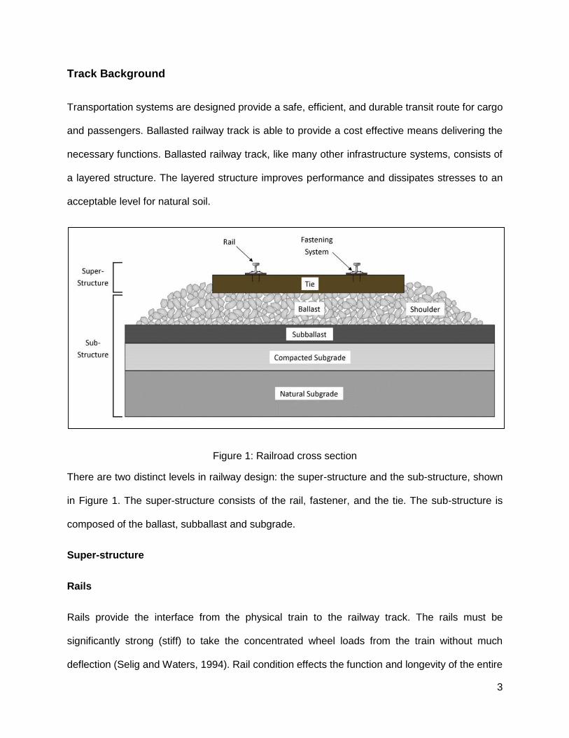
Track Background
Transportation systems are designed provide a safe, efficient, and durable transit route for cargo
and passengers. Ballasted railway track is able to provide a cost effective means delivering the
necessary functions. Ballasted railway track, like many other infrastructure systems, consists of
a layered structure. The layered structure improves performance and dissipates stresses to an
acceptable level for natural soil.
Figure 1: Railroad cross section
There are two distinct levels in railway design: the super-structure and the sub-structure, shown
in Figure 1. The super-structure consists of the rail, fastener, and the tie. The sub-structure is
composed of the ballast, subballast and subgrade.
Super-structure
Rails
Rails provide the interface from the physical train to the railway track. The rails must be
significantly strong (stiff) to take the concentrated wheel loads from the train without much
deflection (Selig and Waters, 1994). Rail condition effects the function and longevity of the entire

4
track structure. If there are defects in the rail, not limited to: cracks, impurities, poor welds, and
jointed sections these can cause stress risers and increased stress and deformation can occur.
A properly functioning rail is integral to the durability of ballasted rail track.
Fasteners
The fasteners connect the rail with the tie. The fastener should resist vertical, lateral, longitudinal,
and overturning movements of the rail (Selig and Waters, 1994). Different fastening systems exist
for both wood and concrete sleepers. Fasteners for wooden ties require a steel plate underneath
the rail to dissipate the load on the tie. For concrete ties, a stiff rubber pad may be required to
stop the degradation from repeated loads on a stiff surface, dampen vibrations, and insulate the
rail.
Ties
Ties are the components of the track structure that are placed at the top of the ballast layer,
perpendicular to the direction of rail. The function of the tie is to take the load from the bottom of
the tie plate (or other fastening system) and distribute that load through the tie to the ballast
structure (Indraratna et al. 2011). For this system to work effectively, each component must
adequately handle the loads and stresses. Ties come in a variety of types and sizes, though the
most common is the wood tie with dimensions of 2.59 m x 0.229 m x 0.178 m (9’ x 9” x 7”) (L x W
x H) (Selig and Waters, 1994). Other types of ties include reinforced concrete, steel, recycled
plastic, tropical hardwood, and composite ties (Indraratna et al. 2011). The target properties of an
effective tie are long life, load-bearing capacity, and minimal defects. For much of the freight
industry and in most US climate regions, standard wood ties meet these requirements and are
often most cost effective (Webb et al. 2012).
5
Sub-structure
Ballast
Ballast is the top layer of the substructure consisting of a select crushed granular material (Selig
and Waters, 1994). The ballast should be high quality rock, but is often governed by location and
economic considerations. No standards exist for ballast, but AREMA offers suggestions for
classifications of ballast. Regardless ballast should perform many functions, but the most
important are:
1. Resist vertical, lateral, and longitudinal forces applied to the sleepers through the track
2. Provide some resiliency and energy absorption of traffic
3. Provide immediate drainage of water
4. Reduce pressure from the tie bearing area to acceptable levels for the underlying layers.
(Selig and Waters, 1994; Indraratna el al. 2011)
Subballast
The second layer in the substructure is the subballast. Typically a finer gradation than the ballast,
subballast performs three main tasks.
1. Reduce traffic stress at the bottom of the ballast layer to an acceptable level for the
subgrade
2. Extent subgrade frost protection
3. Assist draining while preventing migration of ballast and/or subgrade into each other,
subballast acts as a filter between these two layer
(Selig and Waters, 1994; Hay, 1981)

6
Subgrade
Subgrade refers to the natural soil of the area and when constructing sections of track the
engineering properties of the subgrade must be known. Typically the top layer of subgrade is
compacted per specifications to allow increased bearing capacity and shear strength. In areas
where soft or weak soil are found, further design and remediation techniques may be used to
increase the soil strength to an acceptable level. As was true for ballast and subballast, water
drainage is a key factor when designing a track section. Drainage ditches, culverts, and vegetation
management strategies need to be assessed, as any unwanted moisture retention can lead to
track instability and major damage to track and train components (Hesse, 2013). Track structure
can be modified by the use of geosynthetics to improve the performance of different aspects of
the track.
Fouling
Selig and Waters (1994) defined fouling as the percent mass of soil particles passing through a
4.75 mm (#4) sieve with the percent of particles passing a 0.075 mm (#200) sieve. Ballast exists
in a wide range of fouling indices from clean (FI = 0) to heavily fouled (FI = 40).
𝑭𝑰 = 𝑷𝟒 + 𝑷𝟐𝟎𝟎
𝐹𝐼 < 1 − 𝐶𝑙𝑒𝑎𝑛 𝐵𝑎𝑙𝑙𝑎𝑠𝑡
1 ≤ 𝐹𝐼 ≤ 10 − 𝑀𝑜𝑑𝑒𝑟𝑎𝑡𝑒𝑙𝑦 𝐶𝑙𝑒𝑎𝑛 𝐵𝑎𝑙𝑙𝑎𝑠𝑡
10 ≤ 𝐹𝐼 ≤ 20 − 𝑀𝑜𝑑𝑒𝑟𝑎𝑡𝑒𝑙𝑦 𝐹𝑜𝑢𝑙𝑒𝑑 𝐵𝑎𝑙𝑙𝑎𝑠𝑡
20 ≤ 𝐹𝐼 ≤ 40 − 𝑆𝑖𝑔𝑛𝑖𝑓𝑖𝑐𝑎𝑛𝑡𝑙𝑦 𝐹𝑜𝑢𝑙𝑒𝑑 𝐵𝑎𝑙𝑙𝑎𝑠𝑡
𝐹𝐼 ≥ 40 − 𝐻𝑖𝑔ℎ𝑙𝑦 𝐹𝑜𝑢𝑙𝑒𝑑

7
Track Design & Maintenance
There are two popular types of railroad tracks in use today: slab tracks and ballasted tracks. Both
tracks offer advantages and disadvantages. What follows is a summary of Buddhima Indraratna’s
Advanced Rail Technology-Ballasted Track.
Ballasted track offers low construction costs, and in many instances can use material sources
nearby. The design and construction process of the track is simple. The maintenance equipment
and processes involved are also simple. During precipitation events the ballasted track allows
rapid drainage of water from the track structure, water is detrimental to soil performance. The
main disadvantage to ballasted railroad track is maintenance. Ballast rocks degrade and get
fouled over time. This causes unacceptable deformation in the track superstructure. Degradation
and fouling also reduce the pore size of ballast, reducing hydraulic conductivity.
Slab track are essentially slabs of precast or cast-in-place concrete that support the railroad.
These tracks are more suitable for high speed transit and high intensity rail lines where shut-down
for maintenance would impact the users considerably.
In North American the American Railway Engineering and Maintenance of Way Association
(AREMA) publishes an Engineering Manual that provides methods and guidance to construct a
railroad. The methods include calculating aggregate layer thicknesses and the stresses imposed
from train loadings. Train loads are dynamic, but for most analysis the train load is treated as a
quasi-static load. Although the methods are vast simplifications of loads and stress distribution, it
is an acceptable method to design tracks.
Ballast Layer Determination
To determine ballast layer thickness, four methods provided in the AREMA manual are: The
Talbot Equation, Japanese National Railways Equation, Boussinesq Equation, and the Love

8
Equation. These methods all involve ballast layer thicknesses, contact stresses, and interface
stresses (ballast-subballast) a representation can be seen in Figure 2.
Figure 2: Stress Distribution (Selig and Waters, 1994)
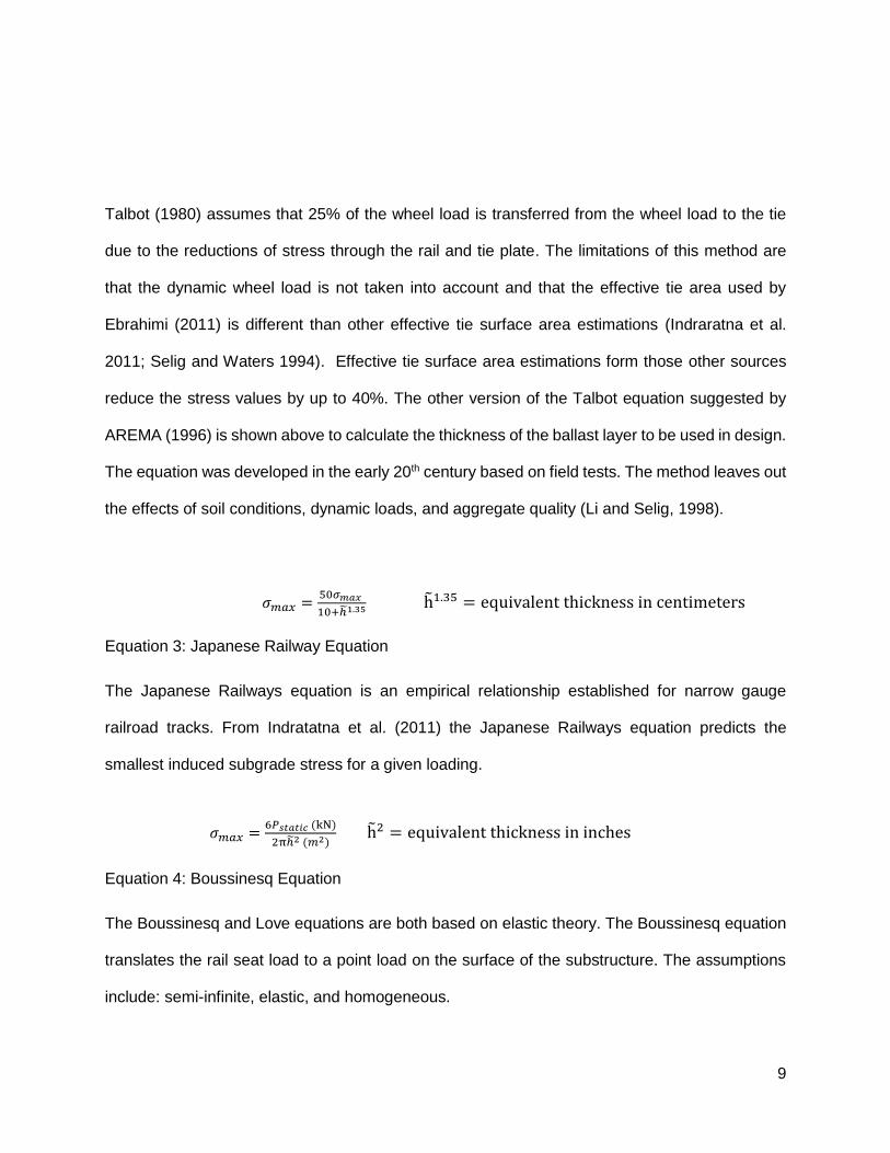
The Talbot Reductions method involves taking the gross weight of the car in kN and calculating
the static wheel load at the point of contact on the rail in kN. The stress under the tie at the tie-
ballast interface is calculated by the following equation:
𝜎𝑚𝑎𝑥 =Wheel Load (kN)
Effective Tie Surface Area (𝑚2)∗ 𝑇𝑎𝑙𝑏𝑜𝑡 𝑅𝑒𝑑𝑢𝑐𝑡𝑖𝑜𝑛
Equation 1: Talbot Equation
𝐻 = 0.24 (𝑃𝑚
𝑃𝑠)
0.8
Equation 2: Talbot Equation
𝐻 = 𝑔𝑟𝑎𝑛𝑢𝑙𝑎𝑟 𝑙𝑎𝑦𝑒𝑟 𝑡ℎ𝑖𝑐𝑘𝑛𝑒𝑠𝑠 (𝑚)
𝑃𝑚 = 𝑣𝑒𝑟𝑡𝑖𝑐𝑎𝑙 𝑠𝑡𝑟𝑒𝑠𝑠 𝑎𝑝𝑝𝑙𝑖𝑒𝑑 𝑜𝑛 𝑡ℎ𝑒 𝑏𝑎𝑙𝑙𝑎𝑠𝑡 𝑠𝑢𝑟𝑓𝑎𝑐𝑒
𝑃𝑠 = 𝐴𝑙𝑙𝑜𝑤𝑎𝑏𝑙𝑒 𝑠𝑢𝑏𝑔𝑟𝑎𝑑𝑒 𝑝𝑟𝑒𝑠𝑠𝑢𝑟𝑒 (138 𝑘𝑃𝑎 𝑟𝑒𝑐𝑜𝑚𝑚𝑒𝑛𝑑𝑒𝑑 𝑏𝑦 𝐴𝑅𝐸𝑀𝐴 (1996)
9
Talbot (1980) assumes that 25% of the wheel load is transferred from the wheel load to the tie
due to the reductions of stress through the rail and tie plate. The limitations of this method are
that the dynamic wheel load is not taken into account and that the effective tie area used by
Ebrahimi (2011) is different than other effective tie surface area estimations (Indraratna et al.
2011; Selig and Waters 1994). Effective tie surface area estimations form those other sources
reduce the stress values by up to 40%. The other version of the Talbot equation suggested by
AREMA (1996) is shown above to calculate the thickness of the ballast layer to be used in design.
The equation was developed in the early 20th century based on field tests. The method leaves out
the effects of soil conditions, dynamic loads, and aggregate quality (Li and Selig, 1998).
𝜎𝑚𝑎𝑥 =50𝜎𝑚𝑎𝑥
10+ℎ1.35 h1.35 = equivalent thickness in centimeters
Equation 3: Japanese Railway Equation
The Japanese Railways equation is an empirical relationship established for narrow gauge
railroad tracks. From Indratatna et al. (2011) the Japanese Railways equation predicts the
smallest induced subgrade stress for a given loading.
𝜎𝑚𝑎𝑥 =6𝑃𝑠𝑡𝑎𝑡𝑖𝑐 (kN)
2πℎ2 (𝑚2) h2 = equivalent thickness in inches
Equation 4: Boussinesq Equation
The Boussinesq and Love equations are both based on elastic theory. The Boussinesq equation
translates the rail seat load to a point load on the surface of the substructure. The assumptions
include: semi-infinite, elastic, and homogeneous.

10
𝜎𝑚𝑎𝑥 =2𝑃𝑠𝑡𝑎𝑡
𝐴𝑠𝑏(𝐹𝑆)
Equation 5: Love Equation
max = Sleeper-ballast contact stress
Pstat = Static rail seat load (Assumed to be 50% of the static wheel load (Indraratna et al.
2011)
Asb = Effective area of tie under rail seat (assumed to be 1/3 the area under the tie)
FS = Factor of safety
The Love equation is a simple model for predicting sleeper ballast contact stress if the tie is
represented as a uniform pressure on a circular area (Indraratna et al. 2011; Chen and Saleeb,
1982; Talbot, 1980). The equation is detailed above. The main limitations of this method are the
dynamic rail load is not taken into account and the factor of safety chosen greatly influences the
output. The assumption of a homogeneous half space also limits the validity of the results. Train
loading and granular thickness has a large impact of the performance of the railroad in both ballast
and foundation soils.
Dingqing Li and Ernest T. Selig (1998) Method for Railroad Track Foundation Design
This two-part installment reviews the development of a new track foundation design and then the
application of the design for use. Although almost 20 years old, the author believes it provides a
good foundation of understanding for track design. One of the major factors of railroad
performance is the subgrade on which the track structure is built. With little confining stresses
toward the surface of the subgrade, high deviatoric stresses occur. Two approaches are
investigated to reduce the deviatoric stress on the subgrade: improve subgrade soil strength and
reduce the deviator stress transferred to the subgrade (increasing granular thickness). Increasing
thickness decreases the deviator stress on any point of the subgrade due to the increase of height.
It also increases the effective bearing area of the train load.

11
The goal of railroad design is to create a system of granular layers that decrease the deviator
stress to an acceptable level, so the subgrade will not excessively deform or show signs of
progressive (cyclic) shear failure. Increasing granular thickness is a viable option for many
maintenance events, but increasing ballast height in certain sections requires significant amounts
of ballast and design to match elevations correctly.

12
HMA Underlayment
Another method of improving railroad track performance is the use of an asphalt underlayment
underneath the ballast layer. This hot mix asphalt (HMA) layer replaces the subballast layer to
increase multiple aspects of the substructure system.
Distribute pressures more uniformly to subgrade
Weatherproof the subgrade
Provide a barrier and surface to assist positive drainage
A resilient layer between the ballast and subgrade to decrease likelihood of
pumping without sacrificing track stiffness
(Rose et al. 2000)
The HMA layer is designed to be a plastic mix with air voids of 1% - 3% and a compacted (in situ)
air voids of less than 5%. Aggregate size may be increased to accept a particle size of 25 – 37
mm, along with the binder content increased 0.5% above the recommended highway application
(Rose et al. 2000). The asphalt mat typically is between 125 mm to 150 mm thick, but in situations
where poor subgrade exists, the thickness may be increased to 200 mm - 300 mm. HMA
underlayment is a costly procedure, and costs can be between $41 to $69 per meter of track ($56
to $93 adjusted prices from 2000 – 2015). The price of HMA increased significantly in 2007
(Hassan, 2009).
An asphalt layer with a width of approximately 3.5 m, with a higher elastic modulus than un-
cemented aggregate will distribute the load over a larger area. This will decrease the pressure
felt by the subgrade, allowing potentially higher axle loads or increased traffic on a section of track
that previously would not be capable. Some concerns exist with HMA underlayment which are
primarily aging/oxidation and cracking. With increasing stiffness over time, HMA is more likely to

13
develop a crack under repeated stress. This crack would allow water to infiltrate, and potentially
lead to subgrade pumping, reducing the effectiveness of the method.
Maintenance Methods
Over time due to static and cyclic loading on railroad tracks permanent deformation occurs.
Sections where this deformation occur are deceptively small, but cause local stress risers that
result in a compounding effect of deformation and spread of deformation (Indraratna et al., 2011).
To maintain operational speeds and ride quality periodic maintenance must be conducted. Ballast
is one of the few controllable variables in maintenance activities, and is responsible for controlling
surface geometry (Indraratna et al., 2011). Considerable cost is incurred when maintenance is
conducted: materials, labor, machine time, mobilization, contracting services, safety, permitting,
and inspection and records.
Typically track/ballast maintenance activities consist of tamping, stone blowing, undercutting and
ballast addition. Ballast tamping consists of a machine that clamps onto the rails, adjusts the
tracks to the desired elevation/super elevation, and then uses vibratory probes to fill the created
void spaces underneath. This method is an effective method for adjusting track geometry, but the
vibratory squeezing has detrimental effects on the ballast. Ballast becomes looser in some areas
(density change) and ballast particles are broken and rearranged (Indraratna et al., 2011). The
ballast particles will have to readjust again after tamping to achieve the necessary interlock to
resist further deformation.
Stone blowing is an automated technique that also brings railway track to a desired elevation.
After time, a void forms underneath the tie from cyclic train loading. This void is undesirable, and
causes decreased performance. Stone blowing is a pneumatic technique that lifts the rail track to
a desired elevation then injects ballast rocks into the void underneath the tie. This restores
geometry and decreases the track deformation under cyclic load (Indraratna et al., 2011).

14
Undercutting is a more aggressive approach to ballast maintenance. This technique is also used
to remove and replace entire sections of fouled ballast with new clean ballast. An undercutting
removes ballast from underneath the track, removes the fines, and places the cleaned ballast
back underneath the track. Then additional ballast is added, if needed, and the track geometry is
corrected possibly by tamping. The fines left over from sieving the ballast are either disposed of,
or used to make new embankments or add to existing ones (Marsh, 2015).
Additional types of maintenance or remedial techniques have been used to fix problem sections
of track. The solutions include geosynthetics, stone columns, silicate grouts, lime slurry injections,
HMA layers (Indratana 2011; Alrulrajah et al. 2008; Brill and Hussin, 1992, Rose et al. 2005).
Mixed reviews of effectiveness has been shown. In tangent track geosythetic usage as well as
traditional soil grout injections has been effective (Indrartana 2011; Brill and Hussin 1992; Li and
Davis, 2005). At bridge approaches the remedies intended to strengthen the subgrade may not
be effective if they do not produce a consistent track stiffness (Li and Davis, 2005). Of four sites
investigated most of the deformation at bridge approaches occurred from the ballast and
subballast layers even with geogrid, cement stabilization or HMA layers improving the stiffness
(Li and Davis, 2005)
The listed maintenance techniques are costly and energy intensive. Track shutdowns and
scheduling are required to conduct a maintenance event and install these remedial measures.
Interviews and Experience
Track design is often idealized and subpar material is used because there is no other choice.
Information gathered through conversations from engineers and project managers working for
railroads in Wisconsin and Illinois indicate that sometimes traditional track layer structure (ballast,
subballast, and subgrade) is not attainable. Regional railroads have to invest more money in ties,

15
bridges and rail to keep operational speeds at a reasonable level. Ballast becomes a secondary
issue and only during larger rehabilitation projects does ballast renewal become important.
The initiative of returning abandoned railroad track back to service is a complex issue. Railroads
of yesteryear often did not include subballast and were frequently constructed on poor soils. This
lead to a poorly draining track structure, that may have unacceptable tie conditions, poor rail, and
multiple crossings that need to be replaced. When maintenance is required undercutting is a
common method to alleviate these problems. A common procedure to rehabilitate older tracks is
as follows (Marsh and Schaalma, 2015):
1. Undercutting the ballast away from under the tie to gain access to the subgrade
2. Removing poor soils and/or placing a layer of geosynthetic/geomesh/filter fabric down
(some track was not formally constructed on sub-ballast)
3. Re-establishing the ballast section.
4. Shoulder cutting these areas to allow previously trapped water to drain out of the
ballast section.

16
Geosynthetic use in Rail Applications
Geosynthetics have been used in infrastructure applications for many years to reinforce, separate,
and provide added drainage capabilities (Koerner, 1998). The infrastructure for rail demands a
robust geosynthetic, which can withstand high pressure from train loading as well as be puncture
resistance from the angular ballast particles. From Koerner (1998) and Fluet (1986) the most
common use of geosynthetics in railroad applications are as follows:
1. Separation in new and old railroads, between in situ soils and ballast
2. Lateral confinement-type reinforcement
3. Lateral drainage from both above and below (pumping)
4. Filtration of the water below to decrease deleterious effects of pumping
Separation of aggregate layers (ballast, subballast, and subgrade) in a rail cross section is integral
to the stability of the system. As a train passes the dynamic load created by the wheel rolling on
the rail can cause intrusion (pumping) of the subgrade into the subballast and ballast layers. Selig
and Waters (1994) quantified the negative effect of fine grain (P4 and P200) material on the ballast
layer. Inhibiting this fine grain material from entering the ballast layer can be accomplished by a
geosynthetic acting as a filter and separator (Koerner, 1998). The added benefit of using a
geosynthetic is also increasing the mechanical properties of the ballast and subballast layer.
The beneficial use of geosynthetics in railroad applications is well known and has been
researched by many (Indraratna 2007; Indraratna 2012; Indraratna 2013; Raymond 2002). Use
of geosynthetic sheets, fabric or grid can lengthen the maintenance cycle on a section of track. A
geogrid installed reduced the 3-month maintenance cycler to a cycle of 3-years Raymond (2002).
Triaxial tests completed by Indratana (2011) have shown that a layer of geocomposite (geogrid
bonded with nonwoven geotextile) performs much better than a standard geogrid. The geogrid
reinforces the ballast layer while the nonwoven geotextile prevents fine intrusion from the
17
subgrade and subballast into the ballast layer. Geosynthetics are a constantly developing area of
technology, geofoams have gained popularity as a light weight fill, compressible inclusion, and
small amplitude wave damping (Horvath, 1994).
Geofoam
A summary from Hovarth (1993) about geofoams follows. Geofoams are typically constructed
from EPS, expanded polystyrene. EPS is formed by taking beads of polystyrene (0.2 mm to 3.0
mm) and manufacturing them in a two-stage process. Pre-expansion, the first-stage, polystyrene
(PS) beads are heated with steam to 80 °C – 110 °C. Heating softens the PS and vaporizes the
pentane within the bead which results in expansion to approximately 50 times the original volume.
The pentane leaving the PS bead causes numerous closed cells to form. The EPS spheres are
then allowed to cool. The second stage consists of placing the loose spheres in a fixed wall mold,
the spheres are re-heated using steam. The molding is typically done under partial vacuum so
the EPS spheres will bond securely. Some dimensional changes occur, shrinking and swelling,
which is a result of cooling and outgassing of the pentane from the EPS cells.
Geofoams are typically prefabricated in geometric shapes (prismatic) prior to installation, but they
can be formed in place. A relatively new technology to railroad applications is the use of rigid
polyurethane foam (RPF) to strengthen the ballast layer and mitigate intrusion of water and fines
from the subballast into the ballast layer (Dolcek, 2013) and improve the mechanical behavior of
clean ballast (Keene, 2012; Woodward, 2014)
18
Polyurethane (URETEK 486)
Similar to traditional EPS geofoam, RPF is a closed cell polymeric foam. The specific RPF used
in this study was supplied by URETEK USA. URETEK USA provided 486STAR-4 BD a two
component polyurethane-resin system developed in conjunction with Bayer Material Science.
URETEK USA Inc. supplied the RPF material in this study and assisted with field injection and
specimen fabrication.
There are two primary chemical components that are required prior to mixing and application of
RPF. As defined in a technical data sheet from Bayer Material Science (2010), the liquid
components are defined as “A” component and “B” component.
For synthesis of thermoset polyurethane-resin foams, the two components (polyester or polyether
polyol and organic polyisocyanate) are proportionately mixed in the presence of a catalyst
(Szycher 1999). The foam structure results from of gas bubble formation during the polyurethane
polymerization process, known as blowing. Gas bubble formation is the result of introducing the
blowing agent (Szycher 1999).
The cellular structure of the RPF is a closed-cell structure as defined by Szycher (1999). For
closed-cell polyurethanes, the percent of closed cells and open cells are determined per ASTM
D6226, which was used in the technical data sheet produced by Bayer Material Science (2010).
The 486STAR-4 BD possesses a closed-cell content of 90%. Further investigation and techniques
are needed for determining the closed-cell content of the RPF within the PSB composite. Closed-
cell content may provide further understanding of overall RPF bonding properties and mechanical
behavior. The higher the open-cell content (i.e., inverse of closed-cell content), the more the foam
acts like a semi-rigid (flexible) foam. In the case of rigid-foam, where mechanical properties such
as high strength and stiffness are intended, high content closed-cell foam is ideal. However, the
density of the polyurethane is also important for the mechanical characteristics of the foam, as

19
the density of the foam increases the strength, hardness, and resistance to fatigue all increase
(Randall and Lee 2002; Oertel 1985). Consequently, polyurethane may possess a density that
would be sufficient in the case of rigid-foam, but high open-cell content would result in mechanical
properties that are substandard for the intended design of a rigid-foam.
Polyurethane in Rail
Although polyurethane is a non-traditional maintenance approach, use is increasing in rail
infrastructure. Polyurethane is appealing because of its rapid application and a short curing time
(Keene, 2012). The appeal of the technology is the geocomposite that is the result of the
combination of polyurethane and ballast; it is has a larger elastic regime than ballast, and
increases the overall strength. This has proven beneficial in laboratory testing conducted by
(Keene, 2012; Woodward, 2014; Dolcek, 2013; Dersch et al., 2010; Boler, 2012).
In Dersch et al. (2010) and Boler (2012), the material used for reinforcement is known as
Elastrotrack®, a rigid-compact type of polyurethane used to coat the ballast particles. Using a
direct-shear box test, the shear strength of the reinforced ballast was measured under varying
confining stresses and polyurethane curing times (up to 14 days). In the study, the shear strength
of the treated ballast specimen was 40-60% greater than uncoated clean ballast. After each of
the direct shear tests, a powdering test was conducted where the amount of breakage was
measured by percent particles passing a 13-mm sieve, the treated ballast samples had 3-5% less
breakage than untreated ballast. Therefore, Dersch et al. (2010) identified that polyurethane
treatment greatly increases shear strength of ballast and reduces breakage of ballast particles
under loading.
The other commercially available is XiTrack™ a flexible polyurethane material that contacts the
ballast and creates a network of ballast particles and the polyurethane composite. Kennedy et al.
(2009) and Woodward et al. (2014) led a study where a full-scale model test was assembled and

20
tested to determine the deformational characteristics of the ballast layer with and without
polyurethane reinforcement. The full-scale model consisted of a superstructure system of several
rails and ties and substructure layer with a subgrade and a ballast layer. In their investigation, the
accumulation of plastic strain in their full-scale model over 500,000 loading repetitions was
measured. The tests were conducted, where loading repetitions applied to the full-scale model
simulate railway traffic loading conditions on the substructure. Kennedy et al. (2009) found that
settlement of the ballast layer in the model was 95-98% less for the treated substructure than
untreated substructure. It was also shown that the track modulus, a stiffness coefficient, were also
improved over an untreated ballast section (Woodward et al. 2014).
Other trials of XiTrack™ have been conducted in laboratory and field settings. Specifically in the
United Kingdom, where XiTrack™ has been applied at junctions, tunnels, and tangent tracks
Woodward et al. (2011), Woodward et al. (2014) and Kennedy et al. (2013). Field verifications of
laboratory findings was crucial for a railroad contractor (Balfour Beatty Inc.), to adopt the
technology and to reduce maintenance costs, XiTrack™ has led to a three time increase in the
speed of deployment of repairs (Heriot Watt). The polyurethane grip reinforcement helps keep
train and track clearance issues in tunnels to a minimum. By creating a robust geocomposite the
clearance issues associated with ballast fouling and soft subgrade soil in a tunnel can be
remediated (Woodward et al. 2011). In Kennedy et al (2013) the XiTrack™ polymer was applied
to a switch and crossing on a West Coast Main Line in the United Kingdom. The polymer
application lasted for 10 years until scheduled track rebuilding was completed. During those 10
years no maintenance was conducted. Previously, maintenance was conducted 3-4 times per
year. This implies a massive reduction in maintenance cycles and cost for this XiTrack™ treated
section of rail (Kennedy et al. (2013)).
A large concern with placement of polyurethane within a railroad structure is maintenance.
Traditional maintenance equipment such as tampers and under cutters could have a problem with

21
a stiff material. In Kennedy et al. (2013) the polymer was removed and no notes were made
whether it was problematic. In previous laboratory work conducted at UW-Madison, the URETEK
polymer was broken by sledge hammers with significant effort, to observe bonding and interfaces.
22
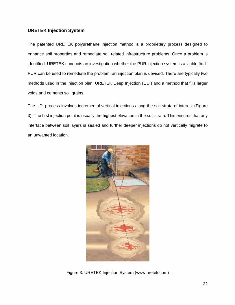
URETEK Injection System
The patented URETEK polyurethane injection method is a proprietary process designed to
enhance soil properties and remediate soil related infrastructure problems. Once a problem is
identified; URETEK conducts an investigation whether the PUR injection system is a viable fix. If
PUR can be used to remediate the problem, an injection plan is devised. There are typically two
methods used in the injection plan: URETEK Deep Injection (UDI) and a method that fills larger
voids and cements soil grains.
The UDI process involves incremental vertical injections along the soil strata of interest (Figure
3). The first injection point is usually the highest elevation in the soil strata. This ensures that any
interface between soil layers is sealed and further deeper injections do not vertically migrate to
an unwanted location.
Figure 3: URETEK Injection System (www.uretek.com)

23
Because of the expansive properties of the injected foam, surface elevations have to be monitored
continuously while the injection is taking place. Expansion or lift, however, is controllable and this
lends PUR injection itself to slab lifting/jacking.
Problem areas such as soft, compressible silts and clays can be remediated by polyurethane
injection (Buzzi et al. 2010). The expanding PUR injection is similar to high pressure cementitious
grouting. Compaction grouting, with traditional slurries, soil is displaced and directly reduces the
volume of the soil voids (El-Kelesh et al. 2012). For traditional grouting methods, to show soil
strength improvement SPT and CPT are used prior to grouting and after curing of the cement
grout (El-Kelesh et al. 2012). The PUR injection typically uses Dynamic Cone Penetrometer data
(DCP) to qualitatively/quantitatively measure soil resistance and penetration indices to show
ground improvement.
The other aspect of PUR injection is the bonding and cementing of soil particles. In soil where
larger voids are found (i.e., gravel) the intrinsic permeability is higher which leads to the PUR
injection infiltrating more soil (Buzzi et al. 2010). In unpublished tests conducted by Warren
(2014), particle bonding has a high correlation with D10 with all other variables held constant. The
quality of bonding between the PUR and items is a function of many variables (Szycher, 1999),
but through many laboratory experiments (Keene, 2012; Dolcek, 2014), full permeation of ballast
voids with polyurethane has increased the mechanical performance of the material.

24
Chapter 2: Decision Making
Life Cycle Cost Analysis Background
For any engineering decision, a critique of the solutions offered to solve a certain problem should
be conducted. In this specific instance, one would decide to which type of maintenance event to
utilize on a section of track. Besides initial cost, time to implement, and performance, there are
tools that exist to help make the decision relevant both in terms of life cycle costs and
environmental impacts. One of these tools is a Life Cycle Cost Analysis (LCCA). A LCCA is a
method for evaluating the total cost of a project, from cradle to grave (Figure 4). LCCA is a tool
for considering all costs of acquiring, owning, and disposing of a railroad track (Angeles, 2011).
Figure 4: Typical LCCA Process (Hsu, 2011)
A product begins its life as a raw material. Whether it be extracted from Earth or created by
manufacturing, these building blocks are the start of a useable product. The next step in the life
cycle process is transforming the material into a useable form for later use, such as crushing and
screening rocks for specific gradations of ballast. Transportation may be included at any step, as
material may have to be moved from one location to another. In railroad ballast, the manufacturing

25
of the rock to achieve the proper gradation for new track construction or for maintenance activities
is considered. During a material’s usable lifecycle, performance is expected to degrade once a
critical performance index is reached; an action must be taken to restore the performance. Poor
ballast condition is known to cause delays and increase user costs (Chrismer and Davis, 2000).
The waste created by the products use must also be addressed. Degraded railroad ballast creates
finer grained materials by crushing, (termed fouling), and this accumulation of fines decreases
the performance (Selig and Waters, 1994). During a maintenance event these fine-grained
materials are removed to allow better aggregate interlock and drainage (Indraratna et al., 2011).
Traditional railroad maintenance is a complex procedure, which begins at the initial design of the
transportation system. There are many ways to evaluate a project’s worth, but a LCCA is a
straightforward and easy-to-interpret measure of economic evaluation (Angeles, 2011). Included
in different LCCA methods are the following measures: Net Present Value, Benefit to Cost Ratio,
Internal Rate of Return and Payback Period (Abdelhalim and Kirkham, 2004).
Comparing projects using an LCCA provides insight to which alternatives have the lowest cost of
ownership over a period of time. Sometimes higher initial costs are traded for reduced future costs
(Angeles, 2011). LCCA has been used for evaluation of structural design of bridges for railroads,
which satisfy safety and required level of performance, but have different initial, maintenance,
operation, and service lives. An LCCA may provide a better assessment than just initial and short
term costs for track maintenance.
LCCA in Railroad
Life cycle cost analyses have been used in many aspects of railroad design, specifically, new rail
lines, tunnels and bridges. A European Union-funded research project, Innotrack, developed a
toolbox of solutions to help reduce investments and maintenance related costs. In those solutions
subgrade, rail, and construction processes are examined (Paulsson and Ekber, 2010). One of the

26
methods to reduce costs is to use lime-cement reinforced subgrade soil. This method can be
applied without the need to stop traffic, which leads to decreased track downtime, resulting in both
cost savings (innotrack.eu).
Angeles (2011) presented a detailed study on a railroad tunnel constructed in Switzerland, the
Lotschberg Basis Tunnel. This study consisted of construction costs, tunnel maintenance and
operation costs, and train energy costs. With no information concerning discount rates or benefits
from the tunnel construction, a Net Present Value (NPV) method and sensitivity analysis was
deemed as the best method to analyze the project. In a NPV method analysis cash flows are
documented and then converted to present value. A sensitivity analysis of item cost and discount
rate was conducted. The sensitivity analysis revealed that a cost item with the largest value
always impacts the present value the greatest. The discount rate has a significant effect on the
NPV, but as the discount rate increases, its effect on the NPV lessens.
Nielsen et al. (2013) has shown similar findings to Angeles (2011). Railway bridges are another
facet of railroad infrastructure that receives significant attention. Furthermore, many of the aspects
of a railroad bridge are nearly identical to other infrastructure-purposed bridges. LCCA can be
applied to existing structures as well; specifically, in the maintenance alternatives. Typically,
LCCA are conducted over the lifetime of a project or structure, but it is applicable to simplify the
analysis over a shorter term to analyze element life. Railroad bridges in Australia’s rail network
system can be optimized by a three-point system, one of which includes LCCA. A LCCA
estimation model that could increase the accuracy of cost estimates, and reduce the uncertainty
in estimation, would result in less budget uncertainties.

27
By the nature of construction projects, a significant amount of material is transported and
consumed. Before some of the material is even used, it may have to undergo treatment prior to
its application. All these factors lead to a product that can have significant economic impact
(Henrickson and Horvath, 2000). As of 2006, state DOT officials indicated that at least 80% of the
states (USA) conduct an LCCA during the pavement selection process for roadway projects
(Chan et al. 2008). For public road construction projects, it is common-place to use LCCA. A
LCCA can help justify to the public how and why the road section was constructed with the
selected materials and lifetime. AMTRAK (a public owned, rail-transit company) maintains a
significant portion of railway track across the United States. AMTRAK has had annual renewal
and maintenance cost of $208,000 per track mile. Some European railroads average an
expenditure of $174,000 per main track mile and some individually held, private, railroads had
maintenance costs ranging from $91,000 to $380,000 per main line track mile. (Amtrak Office of
Inspector General, 2009). Maintenance operations are costly and, if a company would like to
examine expenditures and costs, LCCA is a useful tool in doing so.

28
Life Cycle Analysis Background
With an environmentally conscious society, decisions are both economically and environmentally
fueled. Environmental impact of a project can be a large concern for companies, natural resources
have a finite quantity, and conservation of them saves money and potentially harmful pollutants.
A Life Cycle Assessment (LCA) is a tool to examine the associated processes with a product from
the inception to the end of its useable life (Baumann and Tillman, 2004). The LCA has been
recognized as a valuable tool and the International Organization for Standardization (ISO) has
created a guideline for which one can design an LCA for a product, service, or construction.
Shown below in Figure 5 is a typical LCA design backbone.
Figure 5: Typical LCA Construction modified from (wrtassoc.com)

29
An LCA consists of four parts (ISO 2006b)
1. Definition of goal, scope and functional unit
2. Life cycle inventory
3. Life cycle impact assessment
4. Interpretation of the study
The LCA is similar to a LCCA, the LCA is concerned with emissions and environmental impact
and the LCCA is primarily an economic means studying the impact of a project. An accounting
LCA compares multiple products. Studies like this may be used to understand which alternative
is the best choice, and when alternatives are dated (Hsu, 2009). Construction projects and
materials use a considerable amount of the resources humans use today (Hsu, 2009). Products
and construction that are modern, and have the ability to conserve resources are preferred for
modern construction techniques.
New railroad construction and maintenance is an energy-intensive task. Although, railroads are
efficient in conducting maintenance, these events still require time, material and energy. New
construction is especially intensive. For example, steel rails, are recyclable; however, they require
a high amount of energy to repurpose the old goods. Therefore, it would be beneficial if a
maintenance activity could extend the life of the entire structure.
Another facet of conducting an LCA is the uncertainty. Inputs vary by range or distribution and
this has an effect on the final outcome. The distributions and ranges are necessary to determine
how representative the average is after being chosen for analysis (Sonnemann et al. 2002). The
uncertainty can be represented by multiple factors.
1. Parameter uncertainty. The quality of the data collected is dependent on measurement
quality, sample size, and date of the measurements.

30
2. Model uncertainty. If a model has larger uncertainties, the results from the analysis may
be incorrect.
3. Uncertainty due to choices. To conduct and LCA, the operator will have to make choices
as to allocation, transportation, and functional unit.
4. Spatial variability. Data gathered from one region may not be representative of processes
from another locale.
5. Temporal variability. Technology and operations change as time progresses.
(Sonnenman et al., 2002).
Understanding the uncertainty involved in a LCA, and accounting for it, is crucial for understanding
the chosen parameters. Monte Carlo simulation has been used extensively in understanding the
variation and limitations to a LCA. Limitations can be overcome by the use of a Monte Carlo
Simulation. A Monte Carlo Simulation is a method of managing uncertainty in information. The
simulation uses the distribution of the data, a random number generation, and builds a model of
potential results. The results are in the form of a probability distribution, and to generate this
distribution a discrete amount of simulations are conducted. Data fed into the simulation typically
has a distribution itself, with common ones being: normal, lognormal, uniform, and triangular. The
random number generator chooses a point of each distribution, randomly, to sample and create
iterations of the same process, but with different values.
LCA in Railroad Applications
LCA is prevalent in infrastructure construction and roadway design. The applications of LCA in
railroad construction is less widespread. Most LCA’s conducted in the railroad sector pertain to
bridges and transportation by train (Stripple and Uppenberg, 2010; Du, 2012; Du and Karoumi,
2013; Du and Karoumi, 2012).

31
Stripple and Uppenberg (2010) studied the Bothnia Line, a newly constructed single-track railway
in Northern Sweden. Since the beginning of construction, environmental aspects were important.
An Environmental Product Declaration (EPD) was required for construction, in which an LCA was
used. The study was projected for 60 years, which is long, but the timeline was meant to provide
balance between construction, operation, and maintenance. A common functional unit was used
for different models of bridge construction, tunnels, track, operations, and maintenance. For each
one of the impact categories studied, the infrastructure material and construction work accounted
for largest contributors. A payback period is calculated for the CO2 emissions created from the
project. The purpose of the project was to increase efficiency and decrease time spent doing other
activities. The payback period for CO2 emissions was 13 years, and emissions from 60-year life
time work be offset by the increased efficiency.
Railway bridges can be a large infrastructure project especially for a train system that has to
support ever-increasing loads (Du, 2012; Du and Karoumi, 2013; Du and Karoumi, 2014). The
construction of a railroad bridge has been scrutinized using an LCA in this research. The bridge
of interest was located on the Bothnia Line in Sweden. The bridge had a 42 m span. A systematic
approach to analyze new railroad bridge construction is shown while also comparing ballast deck
bridges to concrete fixed slab bridge. The LCA included material manufacturing, construction,
maintenance, usage, and an end-of-life scenario. Using these inputs the ReCiPe method was
chosen for one of the LCA methods to be used to analyze the different categories of interest. In
this study, and the conditions imposed, the fixed slab track bridge was more environmentally
friendly for the categories investigated. Du and Karoumi (2013) acknowledged that past research
has found that traditional ballasted track achieved a better environmental performance. The LCA
method, boundary conditions, and available information is essential to producing repeatable
results.
32
Monte Carlo Simulation
In an LCA, there is uncertain data that will be encountered. To improve the quality of the final data
multiple methods can be used (Bjorklund, 2002). Bjorklund (2002) provides a review of 13
different methods used to improve data in LCA. A commonly used analysis is probabilistic
simulation, or Monte Carlo simulation. With available data concerning the products involved in the
LCA statistical information can be assigned. The Monte Carlo technique uses a large (thousands)
amount of stochastic simulations. The values used for the analysis are chosen randomly from the
input product data distributions. Upon completion an estimate of the probability density function
is formed (Salve, 2008). Another method of visualizing a Monte Carlo simulation is a method that
replaces discrete values with random variable drawn from probability density functions (LaGrega
et al. 1994). Conducting a Monte Carlo simulation provides a probability density function of where
the true value may lie.

33
Chapter 3: Geotechnical Field Investigation
Geotechnical and Geophysical Investigation Overview
On September 18th and 19th, 2014, URETEK engineers and UW-Madison researchers completed
a geotechnical and geophysical investigation on a spur track section in Dayton, Illinois. This track
functions solely to service Wedron Silica and ship fracking sand to larger rail hubs (i.e., Rockford,
IL). Over this 2.4 km (1.5 mile) stretch three problem areas were investigated. The problem areas
were named: ballast section, concrete section, and culvert section to better describe the
characteristics of the site. Herein the three are described with results and interpretations.
Testing Details
The tests completed were designed to identify:
relative strength, soil layer thickness, and material
type. These properties are crucial to methodologies
in track design and URETEK’s injection strategy. The
tests conducted are as follows:
Dynamic cone penetrometer (DCP)
Ground penetrating radar (GPR)
Electrical resistivity (ER)
Sampling with laboratory tests
Time domain reflectometry (TDR)
Figure 6: Ballast site track condition

34
Test Descriptions
Dynamic cone penetrometer (DCP) tests provide a measure of the shear strength in the
underlying soil strata without excavation. Typically an exploration length of 0.80 m (2.6 ft) to 1.50
m (4.9 ft) is achievable with a standard DCP test. URETEK USA has a robust DCP system that
is capable of achieving depths of up to 10 m (32.8 ft). A weight of known mass is dropped a
distance, the force that is created drives a cylindrical cone into the underlying soil strata. The
depth of penetration per blow (mm/blow) provides the measure of the shear strength of the soil
Ground-penetrating radar (GPR) is a geophysical technique that uses a source at the surface to
generate an EM waves that travel down through the subsurface until it reaches a boundary
between materials with contrasting electromagnetic properties (Figure 7). When the EM wave
reaches such interface, some of the wave energy reflects back while some of the energy is
transmitted. The reflected energy travels back to a receiver at the surface where its arrival time
and amplitude are captured.

35
Figure 7: GPR survey technique
GPR data were collected using pulseEKKO PRO system and 200-MHz antennae for the three
sections of the track: ballast section, concrete section, and culvert section. The ballast and culvert
section yielded quality high GPR data. To interpret these data, a set of processing steps were
implemented: time-zero correction, mean spatial filter, median spatial filter, and gain control
function.
Time domain reflectometry (TDR) was used to complement and calibrate GPR models and verify
field conditions. TDR, like GPR, uses the propagation and reflection of EM waves to measure
geomaterial properties such as dielectric permittivity and electrical conductivity along the length
of two metal probes.
Electrical resistivity survey, another geophysical technique, was also used to image the sub-
surface. Imaging relies on the electrical resistance of the soil materials. Different resistances
correlate with different geomaterials (Figure 8). The apparent resistivity is measured through

36
applied current/voltage at the surface to electrodes embedded in the soil. Detecting the changes
in apparent resistivity implies changing conditions in the underlying soil. Different features can be
imaged using this technique: water table, underlying strata, and voids/dense objects.
Figure 8: Geological resistivity ranges (www.eos.ubc.ca)
A SYSCAL KID Switch-24 by IRIS Instruments was used to conduct the electrical resistivity
surveys. A spacing of 2 m (6.6 ft) or 5 m (16.4 ft) was chosen depending on site geometry, 24
electrodes were embedded in the soil at each site. Res2DInv software was used to process the
data.
Sampling techniques were also utilized to collect disturbed soil samples and to ground-truth the
geophysical survey results. Mass samples of in situ ballast from within the ties, shoulder ballast,
and subgrade were taken. These samples are disturbed, but are highly valuable for engineering
property characterization using techniques such as grain size distribution, particle characteristics,
and shear strength. Other samples were also retrieved from the subgrade. Shelby tubes were
driven 0.7 m (2.3 ft) into the soil, capped, and stored for future laboratory testing. These subgrade
samples will be tested for stiffness and strength properties relating to railroad loading.

37
Site Location
Three sites were chosen for
investigation. Two included slope
failures and one was a ballast settlement
problem. Figure 9 shows the northern
boundary of each location. The sections
will now receive the aliases of Ballast
(i.e., the section with ballast problem),
Concrete (i.e., the section with concrete
retaining blocks), and Culvert (i.e., the
section with stone culvert underneath
the rail track).
The mid-point GPS coordinates of the
sections where the location where DCP
tests were conducted. These
coordinates are:
Ballast: 41°24'27.40" N - 88°46'57.29" W
Concrete: 41°23'49.80" N - 88°47'13.10" W
Culvert: 41°23'33.10" N - 88°47'19.00" W
This section of track borders the Fox River north of Dayton, IL. The track in this region has a grade
(South to North) of approximately 1.0%. A detailed survey was conducted using a total station at
the Ballast site and a local grade of 0.5% was determined (Figure 10). No established benchmark
was found, but elevations from the GPS survey were used to establish a baseline elevation above
sea level.
Figure 9: Google Earth image of site locations
N

38
Figure 10: Total station survey data for Ballast site
Ballast Site
The first rail track section investigated was the Ballast site, this site was had the simplest geometry
with no additional structures present (Figure 11). The investigated site was 76 m (250 ft) long,
contained a standard rail gauge (1.44 m – 4.7 ft), and 1.8 m shoulders. This site was surveyed in
detail and contained a 0.5% grade along the 56 m (184 ft) length (Figure 10). The ballast was of
poor condition; multiple ballast types and fines were present.
160.4
160.5
160.6
160.7
160.8
160.9
161
-40 -20 0 20 40
Ele
vati
on
(m
)
Distance (m)

39
Figure 11: Ballast site overview
Dynamic Cone Penetration Results
The DCP test was conducted by URETEK at the midpoint of the section. Results are shown in
Figure 12. The DCP profile exhibits a strong ballast layer followed by a weak layer of
approximately 1 m (3.3 ft). Beyond 2 m (6.5 ft) depth the soil profile exhibits increased resistance
to penetration with depth. The DCP results correlate well with the GPR layer thickness and
sampling conducted at this location; i.e., the refusal at 3.4 m (11.2 ft) agrees well with a horizon
seen in the GPR section.

40
Figure 12: DCP results for Ballast site
Ground Penetration Radar Results
Figure 13 shows a Google Earth image of GPR survey line of the ballast section, boundaries of
ballast section, and location of DCP test. Processed GPR data of the ballast section in Figure 14
indicate the presence of three layer interfaces corresponding to ballast layer, subballast layer,
subgrade layer, and bedrock (stronger subgrade). GPR data exhibits a local dip in a track
substructure which coincides with the settlement zone that spans from the horizontal position of
50 m (164 ft) to 85 m (279 ft). The dip shown in the GPR data indicates potential for accumulation
of soft soil that may be a possible explanation for settlement in this area.
0
0.5
1
1.5
2
2.5
3
3.5
4
0 10 20 30 40 50 60
Dep
th B
elo
w S
urf
ac
e (
m)
Penetration Index (mm/blow)
DCP Test @ M 75.5 (Ballast)

41
Figure 13: GPR survey line
Figure 14: GPR result with DCP overlay

42
Electrical Resistivity Results
Preliminary ER results using a Wenner array in horizontal profiling configuration show low
resistivity’s (6 m – 11 m) in the top 2 m (6.6 ft) of soil (Figure 15). This range of resistivity
associated with clay and organic soil (Figure 8). Groundwater also has similar electrical
resistivities to clay and organic soils, pockets of ponded water were noted at this site. Major
findings included a clayey soil with high water content.
Figure 15: ER section for Ballast site
N
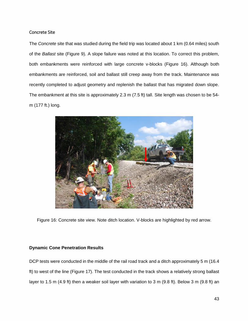
43
Concrete Site
The Concrete site that was studied during the field trip was located about 1 km (0.64 miles) south
of the Ballast site (Figure 9). A slope failure was noted at this location. To correct this problem,
both embankments were reinforced with large concrete v-blocks (Figure 16). Although both
embankments are reinforced, soil and ballast still creep away from the track. Maintenance was
recently completed to adjust geometry and replenish the ballast that has migrated down slope.
The embankment at this site is approximately 2.3 m (7.5 ft) tall. Site length was chosen to be 54-
m (177 ft.) long.
Figure 16: Concrete site view. Note ditch location. V-blocks are highlighted by red arrow.
Dynamic Cone Penetration Results
DCP tests were conducted in the middle of the rail road track and a ditch approximately 5 m (16.4
ft) to west of the line (Figure 17). The test conducted in the track shows a relatively strong ballast
layer to 1.5 m (4.9 ft) then a weaker soil layer with variation to 3 m (9.8 ft). Below 3 m (9.8 ft) an

44
even weaker soil is encountered until refusal at 4.3 m (14.1 ft - Figure 17). Results from the DCP
test conducted in the ditch show similar results (Figure 17 and Figure 18). The top 1 m (3.3 ft) soil
is relatively soft with high penetration indices. Below 1 m (3.3 ft), the soil strengthens and refusal
is at 2.6 m (8.5 ft). The embankment is approximately 2.4 m (7.9 ft) tall. These results correlate
well with where the softer soil is as seen inError! Reference source not found.. The soil and
ballast used to construct the embankment is relatively strong, but when the subgrade (ditch) soil
is reached the strength decreases significantly.

45
Figure 17: DCP results for track test
Figure 18: DCP results for ditch
Figure 19: Vertically corrected DCP results
0
1
2
3
4
5
0 5 10 15 20 25 30De
pth
Be
low
Su
rfa
ce
(m
)
Penetration Index (mm/blow)
DCP Test @ M 75.9 (Concrete) in Track
0
0.5
1
1.5
2
2.5
3
0 10 20 30 40 50 60De
pth
Be
low
Su
rfa
ce
(m
)
Penetration Index (mm/blow)
DCP Test @ M 75.9 in Ditch
0
1
2
3
4
5
0 10 20 30 40 50 60
De
pth
Be
low
Su
rfa
ce
(m
)
Penetration Index (mm/blow)
DCP Test @ M 75.9 Overlay
Track DCP
Ditch DCP (Vertically Corrected)
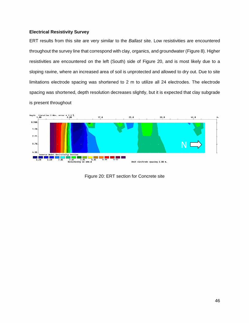
46
Electrical Resistivity Survey
ERT results from this site are very similar to the Ballast site. Low resistivities are encountered
throughout the survey line that correspond with clay, organics, and groundwater (Figure 8). Higher
resistivities are encountered on the left (South) side of Figure 20, and is most likely due to a
sloping ravine, where an increased area of soil is unprotected and allowed to dry out. Due to site
limitations electrode spacing was shortened to 2 m to utilize all 24 electrodes. The electrode
spacing was shortened, depth resolution decreases slightly, but it is expected that clay subgrade
is present throughout
Figure 20: ERT section for Concrete site
N

47
Culvert Site
The Culvert site was the most southerly of the three sites (see coordinates and Figure 4). The rail
line was constructed on a large embankment. The embankment has been failing for many years.
Multiple retaining structures have been constructed to prevent translation of material, but they
have been unsuccessful in stopping movement (Figure 21).
Flowing water is present on the west side of the track, and a culvert is present beneath the track
to aid drainage (Figure 21). A site length of 56 m (183 ft) was chosen at this location.
Figure 21: View of the culvert section.
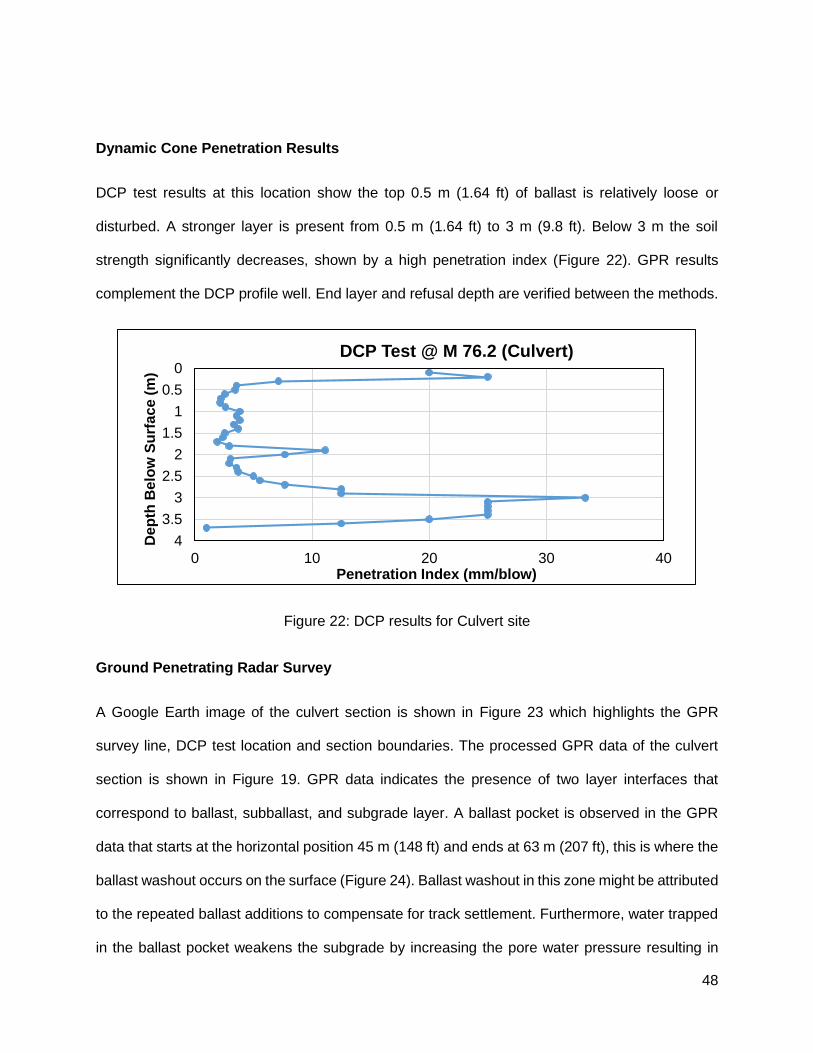
48
Dynamic Cone Penetration Results
DCP test results at this location show the top 0.5 m (1.64 ft) of ballast is relatively loose or
disturbed. A stronger layer is present from 0.5 m (1.64 ft) to 3 m (9.8 ft). Below 3 m the soil
strength significantly decreases, shown by a high penetration index (Figure 22). GPR results
complement the DCP profile well. End layer and refusal depth are verified between the methods.
Figure 22: DCP results for Culvert site
Ground Penetrating Radar Survey
A Google Earth image of the culvert section is shown in Figure 23 which highlights the GPR
survey line, DCP test location and section boundaries. The processed GPR data of the culvert
section is shown in Figure 19. GPR data indicates the presence of two layer interfaces that
correspond to ballast, subballast, and subgrade layer. A ballast pocket is observed in the GPR
data that starts at the horizontal position 45 m (148 ft) and ends at 63 m (207 ft), this is where the
ballast washout occurs on the surface (Figure 24). Ballast washout in this zone might be attributed
to the repeated ballast additions to compensate for track settlement. Furthermore, water trapped
in the ballast pocket weakens the subgrade by increasing the pore water pressure resulting in
0
0.5
1
1.5
2
2.5
3
3.5
4
0 10 20 30 40
De
pth
Be
low
Su
rfa
ce
(m
)
Penetration Index (mm/blow)
DCP Test @ M 76.2 (Culvert)

49
more deformation. A common practice to eliminate this problem is designing a drainage system
to service the ballast pocket.
Figure 23: GPR survey line
Figure 24: GPR result with DCP overlay

50
Electrical Resistivity
ERT results show a section of higher resistivity compared to the other sites surveyed. An electrode
spacing of 5 m (16.4 m) was used here to delineate the entire region of interest. A zone of higher
resistivity is observed where the ballast washout on the surface occurs (Figure 25). Potentially,
the high resistivity seen here is from the ballast particles infiltrating into the subgrade increasing
resistivity. Although the resistivity is higher compared to the other sites, the results still suggest
that a clay soil is present underneath the track with groundwater present (Figure 8).
Figure 25: ERT section for Culvert site
N

51
Bridge Approach - Summary Report
Geophysical Investigation Overview
On April 16, 2015, UW-Madison
researchers completed a geophysical
investigation on two bridge approaches on
a rail section in Dayton, Illinois. The bridge
of interest crosses a small water body,
Indian Creek (Figure 26). Both bridge
approaches show characteristic signs of
deterioration and settlement. It was the goal
of the trip to identify soil strata and potential
failure mechanisms.
Testing Details
The tests completed were designed to identify: soil layer thickness and material type. These
properties are crucial to the injection strategy designed by URETEK the tests conducted are as
follows:
Ground penetrating radar (GPR)
Time domain reflectometry (TDR)
Electrical resistivity tomography (ERT)
Test pit and auger to ground truth geophysical techniques
Figure 26: View of bridge facing north

52
Site Location
The North end of the bridge was
located at Mile Marker 75 (Figure 28).
The coordinates for the two site
locations are as follows and can be
seen in (Figure 27):
North Approach:
41°24'31.9" N - 88°46'55.1" W
41°24'34.1" N - 88°46'54.0" W
South Approach:
41°23'28.2" N - 88°47'56.6" W
41°23'30.6" N - 88°47'55.8" W
Both sides of the bridge approach were delineated to an investigation length of 250 ft (75 m). The
South Approach section overlapped the Ballast section by 30 ft (9 m) from the previous
investigation efforts. The ballast and tie condition on the South Approach was visually poorer than
the North Approach. The surface ballast contained a significant amount of sand, and the wooden
ties were more degraded.
N
Figure 27: Site layout from Google Earth
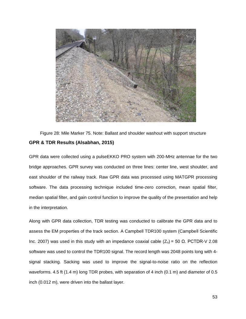
53
Figure 28: Mile Marker 75. Note: Ballast and shoulder washout with support structure
GPR & TDR Results (Alsabhan, 2015)
GPR data were collected using a pulseEKKO PRO system with 200-MHz antennae for the two
bridge approaches. GPR survey was conducted on three lines: center line, west shoulder, and
east shoulder of the railway track. Raw GPR data was processed using MATGPR processing
software. The data processing technique included time-zero correction, mean spatial filter,
median spatial filter, and gain control function to improve the quality of the presentation and help
in the interpretation.
Along with GPR data collection, TDR testing was conducted to calibrate the GPR data and to
assess the EM properties of the track section. A Campbell TDR100 system (Campbell Scientific
Inc. 2007) was used in this study with an impedance coaxial cable (Zo) = 50 Ω. PCTDR-V 2.08
software was used to control the TDR100 signal. The record length was 2048 points long with 4-
signal stacking. Sacking was used to improve the signal-to-noise ratio on the reflection
waveforms. 4.5 ft (1.4 m) long TDR probes, with separation of 4 inch (0.1 m) and diameter of 0.5
inch (0.012 m), were driven into the ballast layer.

54
TDR Results (Alsabhan, 2015)
A typical TDR waveform for the Railway section is shown in Figure 29. The multiple reflections
correspond to substantial differences in the relative dielectric permittivity between the underlying
layers that the EM wave propagates through, shown as the clean ballast and fouled layers in
Figure 29. The first waveform reflection showed a relative dielectric permittivity (εrb) of 3, which is
consistent with relative dielectric permittivity of a ballast layer, whereas the relative dielectric
permittivity (εrf) of the fouled layer was 8. Thus, by incorporating these to calibrate the GPR data
the velocity of the subsurface layer was calculated as 0.15 m/ns. Hence, GPR data was calibrated
with this layer velocity.
Figure 29: TDR waveform with multiple reflections at the DCP location
0
0.2
0.4
0.6
0.8
1
0 1 2 3 4 5 6 7 8 9 10 11 12 13 14 15
Refl
ecti
on
Co
eff
icie
nt
(un
itle
ss)
Distance (m)
Ballast Layer
Fouled Layers
Inflection

55
GPR Survey of the Center Line of the Track
GPR data were collected at the center line of the two bridge approaches. The direction of this
survey was from the north side of the bridge approach to the south side (Figure 30).
Figure 30: GPR survey direction
Processed GPR data of the center line of the two bridge approaches in Figure 31 indicates four
layer interfaces corresponding to a ballast layer, subballast layer, soft subgrade layer, and stiffer
subgrade layer. GPR data shows a local dipping in the subgrade layer close to the bridge
abutments, likely resulting in poor track performance. The GPR layer thickness and sampling
conducted at this location correlate well with the ERT results.
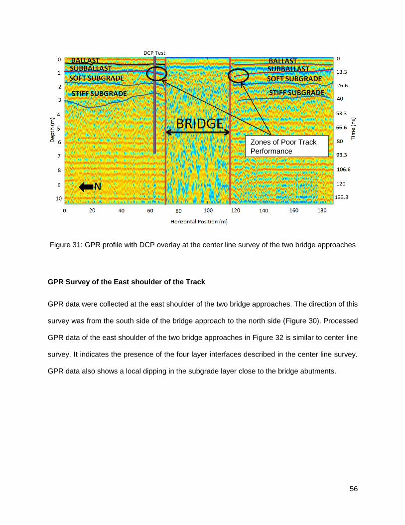
56
Figure 31: GPR profile with DCP overlay at the center line survey of the two bridge approaches
GPR Survey of the East shoulder of the Track
GPR data were collected at the east shoulder of the two bridge approaches. The direction of this
survey was from the south side of the bridge approach to the north side (Figure 30). Processed
GPR data of the east shoulder of the two bridge approaches in Figure 32 is similar to center line
survey. It indicates the presence of the four layer interfaces described in the center line survey.
GPR data also shows a local dipping in the subgrade layer close to the bridge abutments.
Zones of Poor Track
Performance

57
Figure 32: GPR profile with DCP overlay at the east shoulder survey of the two bridge approaches
GPR Survey of the West shoulder of the Track
GPR data were collected at the west shoulder of the two bridge approaches. The direction of this
survey was from the south side of the bridge approach to the north side (Figure 33).
Figure 33: GPR survey direction
Zones of Poor Track
Performance

58
Processed GPR data of the center line of the two bridge approaches in Figure 34 indicates four
layer interfaces corresponding to a ballast layer, subballast layer, soft subgrade layer, and stiffer
subgrade layer. A deep ballast pocket is observed in the GPR data that starts at horizontal station
of 50 ft (15 m), ending at station 115 ft (35 m). GPR data shows a local dipping in the subgrade
layer close to the bridge abutments, likely resulting in poor track performance. The GPR layer
thickness correlate well with sampling conducted at this location correlate as well as the ERT
results.
Figure 34: GPR profile with DCP overlay at the west shoulder survey of the two bridge approaches
Zones of Poor Track
Performance
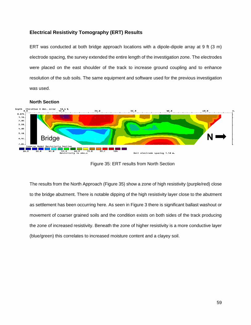
59
Electrical Resistivity Tomography (ERT) Results
ERT was conducted at both bridge approach locations with a dipole-dipole array at 9 ft (3 m)
electrode spacing, the survey extended the entire length of the investigation zone. The electrodes
were placed on the east shoulder of the track to increase ground coupling and to enhance
resolution of the sub soils. The same equipment and software used for the previous investigation
was used.
North Section
The results from the North Approach (Figure 35) show a zone of high resistivity (purple/red) close
to the bridge abutment. There is notable dipping of the high resistivity layer close to the abutment
as settlement has been occurring here. As seen in Figure 3 there is significant ballast washout or
movement of coarser grained soils and the condition exists on both sides of the track producing
the zone of increased resistivity. Beneath the zone of higher resistivity is a more conductive layer
(blue/green) this correlates to increased moisture content and a clayey soil.
N Bridge
Figure 10: ERT results from North Section Figure 35: ERT results from North Section

60
South Section
The South Approach (Figure 36) shows a clearer segregation between higher resistivity materials
(purple/red) and the underlying subgrade (blue/green). At the bridge abutment there is dipping of
the high resistivity materials (ballast/subballast washout) from settlement of the underlying
subgrade. The underlying subgrade soil, which was confirmed to be clay, exhibits expected
resistivity properties. There was 30 ft (9 m) of overlap between this survey and the previous survey
of the Ballast section; the results and observed soil types confirm one another with restivities of
11 m.
Bridge N
Figure 11: ERT results from the South Section Figure 36: ERT Results from the South Section

61
Soil Strata
A small test pit was dug into the shoulder of the North Approach located at a distance 50 ft (15
m) North of the bridge on the West side of the track. Figure 37 shows two views of the pit.
The test pit was dug to assist in ground truthing the geophysical results and to verify the dynamic
cone penetrometer (DCP) test conducted by URETEK in September 2014. At least three
significant layers were found with intermittent layers/pockets of coal burning residue. Figure 38
contains the thicknesses of the layers and the depths below grade.
Figure 37: Test pit pictures from different angles. Picture on the left has rough delineation of soil layers

62
Figure 38: Depths and thicknesses of soil layers
The pit was dug to the top of the coal layer and then a hand auger was used to retrieve samples
until refusal at 170 cm below grade (0 cm = top of the ballast layer). Shown in Figure 39 are the
four soil types encountered in the exploration. The ballast was highly fouled (FI = 42%) primarily
with sand size particles. The subballast aggregate was round, more natural aggregate, with a
significant sand content. The coal layer consisted of smaller (<15 mm) soil grains that were friable
by hand. Following the coal layer the clayey subgrade was found until auger refusal.
Figure 39: From left to right: ballast, subballast, coal material, and subgrade

63
DCP Test
Figure 40: DCP test results
The DCP test conducted by URETEK (Figure 40) shows a strong soil layer from 0 ft – 3 ft (0 m –
0.9 m). This is interpreted as the ballast layer consisting of robust large aggregate particles.
Following the ballast layer from 3 ft – 5.9 ft (0.9 m – 1.8 m) is a zone of weak soil with high
penetration indices. From 1.8 m to the refusal point the penetration index averages approximately
25 mm/blow. From previous DCP tests in this region, the soil encountered in this region is likely
to be a clayey soil with a high water content.
0
1
2
3
4
5
6
7
0 10 20 30 40 50 60
De
pth
Be
low
Su
rfa
ce
(m
)
Penetration Index (mm/blow)
DCP Test @ Bridge Abutment

64
Final Result & Recommendation
GPR results from the shoulders and centerline of the track indicate four unique interfaces relating
to ballast, subballast, soft subgrade and a stiffer subgrade. The layer thicknesses complement
the test pit results and the DCP test. Significant dipping of the ballast and subballast layer is seen
at both bridge approaches indicating settlement and inadequate subgrade (Figure 31, Figure 32,
Figure 34).
The test pit confirms the approximate locations of the high resistivity zone seen in Figure 35 and
Figure 36 from the ERT results. ERT shows at locations closer to the bridge abutment the ballast
and subballast layer is dipping down due to settlement and compression of the clay subgrade
layer beneath. The clay subgrade layer is dipping as well, which indicates that the clay subgrade
is the zone of weakness.
The DCP test (Figure 40) correlates well with the findings from the test pit. The ballast and
subballast layer terminate at approximately 85 cm below grade, then the subgrade soil is present
until auger refusal at 170 cm where the soil strengthens. There may be a small layer of stiffer soil
present at 170 cm, but weak subgrade soil is likely found below.
The interpretation of the results gathered from this investigation that both bridge approaches are
settling due to the poor subgrade beneath the ballast and subballast layers. Additional material
has been added to maintain track alignment, which can be seen in the GPR and ERT data. The
DCP data indicates that the subgrade soil is weak, which complements the interpretations of the
other tests and our interpretation.

65
Laboratory Analyses
Multiple ballast samples were collected during the site visit. There ballast samples were taken
from the top of ballast layer to 5 cm (2 in) below the tie. Upon arrival at the laboratory samples
were oven dried, then a sieve analysis was conducted in accordance to ASTM D422 (Figure 41).
A sealed sample was also taken at each location at the bottom of tie to estimate in situ water
content (Table 1). Increased water content has been correlated to increased deformation in the
ballast layer.
The fouling index is the percentage by weight of particles passing the #4 sieve (4.75 mm) in
addition to the amount passing the #200 sieve (0.075 mm) (Selig and Waters, 1994).
Equation 6: Fouling Index (Selig and Waters, 1994)
𝑭𝑰 = 𝑷𝟒 + 𝑷𝟐𝟎𝟎
𝐹𝐼 < 1 − 𝐶𝑙𝑒𝑎𝑛 𝐵𝑎𝑙𝑙𝑎𝑠𝑡
1 ≤ 𝐹𝐼 ≤ 10 − 𝑀𝑜𝑑𝑒𝑟𝑎𝑡𝑒𝑙𝑦 𝐶𝑙𝑒𝑎𝑛 𝐵𝑎𝑙𝑙𝑎𝑠𝑡
10 ≤ 𝐹𝐼 ≤ 20 − 𝑀𝑜𝑑𝑒𝑟𝑎𝑡𝑒𝑙𝑦 𝐹𝑜𝑢𝑙𝑒𝑑 𝐵𝑎𝑙𝑙𝑎𝑠𝑡
20 ≤ 𝐹𝐼 ≤ 40 − 𝑆𝑖𝑔𝑛𝑖𝑓𝑖𝑐𝑎𝑛𝑡𝑙𝑦 𝐹𝑜𝑢𝑙𝑒𝑑 𝐵𝑎𝑙𝑙𝑎𝑠𝑡
𝐹𝐼 ≥ 40 − 𝐻𝑖𝑔ℎ𝑙𝑦 𝐹𝑜𝑢𝑙𝑒𝑑
66
Figure 41: Grain size distributions
Table 1: Summary table for ballast condition
Sample Location Fouling Index Water Content
Concrete DCP Site 3.1% N/A
Culvert DCP Site 17.9% N/A
Ballast Site Location 1 42.3% 7.9%
Ballast Site Location 1 - Shoulder 1.7% N/A
Ballast Site Location 2 20.7% 9.0%
Ballast Site Location 3 25.2% 6.2%
Ballast sampled at the Dayton Dip has a range from moderately clean ballast to highly fouled
ballast (Table 1). The highest fouling levels are present in the at the Ballast site, where the most
0%
10%
20%
30%
40%
50%
60%
70%
80%
90%
100%
0.010.1110100
Pe
rce
nt
Pa
ss
ing
(%
)
Particle size (mm)
Ballast Grain Size Distributions
Concrete DCP Site Culvert DCP Site
Ballast Site Location 1 Ballast Site Location 1 - Shoulder
Ballast Site Location 2 Ballast Site Location 3
Arema 4a Arema 5

67
significant vertical (1-D) settlement has occurred. Increased fouling levels promote water retention
and amplified vertical deformation compared to clean ballast.
Figure 42: Cyclic triaxial ballast test results
A large (150 kg) amount of ballast was retrieved from the Ballast section and a cyclic traxial test
was conducted at two different deviatoric stresses. The results can be seen in Figure 42 and the
properties of the test can be viewed in Table 2. Further discussion is in the analysis section.
Table 2: Ballast properties
Sample USCS Density (kg/m3)
Porosity Fouling Index
Water Content
Ballast GP 1966 40 % 22 % 9.5%
0.00%
0.20%
0.40%
0.60%
0.80%
1.00%
1.20%
1.40%
1.60%
1.80%
0 100000 200000 300000 400000
Pla
sti
c S
tra
in (
%)
Loading Cycles
Cyclic Triaxial Ballast Test
300 kPa
400 kPa

68
Figure 43: Subgrade grain size distribution
Table 3: Subgrade engineering properties
Sample LL PI USCS Density (kg/m3)
Porosity Water
Content
19 m Subgrade 63 36 Fat Clay with Sand 1,870 33% 25.4%
50 m Subgrade 51 38 Sandy Fat Clay 1,860 33% 24.5%
0
10
20
30
40
50
60
70
80
90
100
0.0010.010.1110100
Pe
rce
nt
Pa
ss
ing
(%
)
Diameter (mm)
Subgrade GSD
19 m Subgrade
50 m Subgrade

69
Figure 44: Subgrade consolidation curves
Multiple Shelby tubes were driven into the subgrade at the ballast section. ASTM D422 was
followed for the particle size distribution seen in Figure 43. The corresponding engineering
properties and soil classification are in Table 3. Upon examination during the extraction of the
Shelby tube samples, there were ballast particles intermixed at short intervals. Carving a sample
with the necessary dimensions (2H: 1V) for triaxial testing proved difficult, with ballast particles
intermixed at random intervals. A consolidation was conducted instead because of the sample
size requirement. The consolidation curve (Figure 44) shows a lightly over consolidated clay. The
different loads applied correspond to different geostatic and train stresses with varying granular
layer thicknesses. The analysis of the results are included in the following analysis section.
0
0.1
0.2
0.3
0.4
0.5
0.6
0.001 0.01 0.1 1 10 100 1000
Vo
id R
ati
o (
e)
Stress (kPa)
Subgrade Consolidation
35 m Subgrade Sample
50 m Subgrade Sample

70
Discussion of Field Results
Failure Mechanisms
Track constructed on soft soil often has the problem of progressive shear failure of the subgrade
and excessive ballast deformation (Figure 45) (Li and Selig, 1998; Hay, 1981). High traffic loads
(frac sand) and poor drainage exacerbate this problem along with inadequate layer thicknesses.
Most of the failures occur on fine grained soils with a high clay content (Li and Selig, 1998). The
Ballast section specimens have a high clay content with in situ water contents of 25%. Seen in
Figure 46 from the site the heave of the soils on the sides of the track is present indicating shear
failure. There is also water present on the surface outside the heave zones. Excess ballast
deformation is not mutually exclusive from subgrade failure, one complements the other. Water
management and increased granular layer thickness are methods to improve this problem.
Figure 45: Failure Mechanisms by Li and Selig, 1998 and Hay (1981)

71
Bridge Approach Settlement
Bridge approach settlement is a complex issue, which is a function of many factors. Isolating the
significant problems is difficult, but reasonable estimates of the failure mechanism can be made
at this location made using the geotechnical and geophysical information. In railroad bridge
approaches three main conditions exist that cause excessive settlement:
1. Large change in track stiffness from change in track structure (ballast – Timber
Bridge). This leads to uneven track deflections under moving loads, creasing a
dynamic interaction with the track. The dynamic interaction leads to even higher forces
on the approach. (Li and Davis, 2005; Kerr and Moroney 1993; Frohling et al. 1995;
Hunt, 1997)
Figure 46: Subgrade failure

72
2. The ballast approach settles more, by inherent material properties and underlying soil
layers. This can produce and uneven profile and differential settlement, increasing
dynamic interaction between the passing train and the substructure (Li and Davis,
2005)
3. Poor quality fill and construction. This includes embankment fill, poor drainage,
inadequate consolidation and compaction. (Li and Davis, 1995)
The data gathered at the bridge approach relates to the soil layers, relative water content, and
approach settlement. The GPR data indicates that the ballast, subballast, and subgrade materials
are all settling at the bridge abutment. All the layers are failing in unison, indicating that the bottom
layer is most likely the cause of the failure. The bottom layer according to the ERT data is a low
resistivity (high conductivity) area, this corresponds to wet clayey soil. Clayey soil under static
load exhibits creep behavior and settlement. Creep is the accumulation of time-dependent shear
strain under sustained shear stress (Mitchell, 1993). A change in track stiffness, without a
displacement change, would lead to a 6% greater dynamic load (Li and Davis, 2005). Settlement
of the approach, along with the stiffness change can lead to increasing high dynamic loads. The
dynamic loads caused by this are approximately 1.5 to 3 times the static load (Nicks, 2009; Davis
et al. 2003). Subgrade has the largest influence on track modulus (stiffness) (Selig and Waters,
1994). The weak subgrade with the high dynamic loading encountered at the bridge approaches
leads to a poor situation. Figure 47 shows the South Approach.

73
Figure 47: South Approach
GPR Discussion
Ground penetrating radar (GPR) is intended to provide images of the railway substructure, to
evaluate its condition, and detect ballast fouling at critical sections of the track. Narayanat et al.
(1999) performed GPR survey on track substructure using three ground-coupled GPR antennae
at 100, 400, and 900-MHz. The data collected with the 900-MHz antennae showed a strong
surface reflection with very little information about the subsurface. Thus, due to the difficulty in
maintaining the proper distance of the 900-MHz antenna within one-eighth of its wavelength (4
cm) above the ground so that the proper coupling of the antenna to the ground is achieved, it was
determined data was unreliable for this application. The results of the 400-MHz antennae were
better when estimating the depth of the subsurface layers while the 100-MHz antennae was

74
better in identifying anomalies, such as water pockets, at deeper depths, compared to the 400-
MHz system.
During the investigation GPR data was collected using a 200-MHz antennae. A co-worker of the
department, whose specialty is GPR, when processed the raw data using MATGPR. The
processing included time-zero correction, mean spatial, filter, median spatial filter, and gain
control. Processed GPR data of the ballast section in Figure 14 indicates three layer interfaces
corresponding to ballast layer, subballast layer, subgrade layer, and bedrock. GPR data shows a
local dip in the track substructure coincides approximately with the settlement zone that spans
from the horizontal position of 50 m to 85 m. This dip shown in the GPR data indicates potential
for accumulation of soft soil that might be responsible for the local settlement of the rail track.
Weak, faint or absence of clear traces in the GPR data that indicate that the layer interface may
be more gradual than discrete. This can be used to identify fouling of the ballast layer, and how
much clean ballast exists in the track.
ER
A Wenner and Dipole-Dipole arrays were used for the exploration of the subsurface. The electrical
resistivity mapping/tomography was carried out along the tracks, where the shoulder of the ballast
stopped. This allowed access to the subgrade, electrode connection with dry ballast proves
problematic, but the subgrade provides insight into what the railroad embankment was
constructed above. For soils the resistivity depends on many factors: porosity, saturation, pore
fluid, and soil grains (Abu-Hassanein et al., 1996).
Electrical resistivity of 10 clays studied in Abu-Hassanein et al. (1996) varied from 4.8 m – 28.97
m. From the results shown previously, the ranges of resistivity predominately lie in this range.
The measurements of electrical resistivity will be affected by the size of the coarse fraction (Abu-
Hassanein et al., 1996). As seen in Figure 25, where the ballast washout and slope failure occurs,
75
the resistivity increases. Ballast has a much larger resistivity than clay, and from sampling was
shown to be mixed with the clay subgrade.
At the bridge approaches, there is a clear segregation between the coarse grained material (i.e.,
ballast and subballast) and the underlying subgrade soils. There is a dip or dipping ballast layer
on both sides of the bridge approach. This indicates that the subgrade, wet clayey, is likely the
source of failure. The investigation sites of the South Approach and the Ballast section overlap
by 9 m. In those 9 m, the results from both investigations show near identical results (7 m – 11
m). This verified method and material encountered in this location (Figure 15 & Figure 36).
Donohue et al. (2010) used ERT on a railway embankment failure in Ireland. Although in a
different country, similar equipment and software was used to collect the data. The ERT profiles
developed for the embankment failure show a similar problem to what is encountered in the
Dayton Dip. The ERT figures show a deposit of silt/clay near the surface. Ballast has been added
around the area of failure, suggesting that ballast additions were used to offset the settlement.
ERT results were verified with MASW and GPR, similar profiles were seen. The presence of a
low strength, high compressibility soft clay under the embankment construction was deemed to
be the major cause of failure in this railroad embankment (Donohue et al. 2010). The ERT method
was able to capture the extent of the clay area, and accurately identify it by the sharp contrast
with the other materials used in railroad construction.

76
Geotechnical Field Methods
Field testing methods of measuring in situ strength of railroad beds differ in measuring the entire
tracks response or measuring individual soil layers. Measuring the railroad tracks total response
to a load is referred to as the track modulus. The track modulus can be measured in a few ways:
1. Single point load test
2. Deflection basin test
3. Multiple axle vehicle load test (Selig and Waters, 1994)
4. Geophones (Priest and Powrie, 2009)
The track modulus is essentially a spring constant (F/L/L). The higher the track modulus, the more
force it takes to vertically displace the railroad track. The track modulus should be in a range of
14-69 N/mm/mm and it should neither be too high, nor too low (Selig and Li, 1994). A modulus
that is too low is a safety concern while a modulus that is considerable higher sacrifices ride
quality.
Track modulus measurements can be made by using rolling stock, remotely using monitoring
techniques, or by a smaller apparatus operated by hand. A concern with measuring track modulus
is that the parameter is representative of the entire structure and not discrete layers of soil. This
can be misleading to which part of the railway structure is deforming, and cannot consider their
individuals impacts (Selig and Waters, 1994)
Other methods exist for measuring discrete soil layer properties in a railway track structure. Vane
shear, cone penetration, flat dilatometers, standard penetration, and dynamic cone penetration
(DCP) are just a few of the semi-intrusive methods used for railroad design purposes. These
methods will provide strength or blow counts for soil layers with can be used to determine soil
layers.

77
Dynamic cone penetrometers
DCP were originally designed for use in flexible pavement systems. They are lightweight and
mobile, resulting in a test that is easy to use and transport. A typical lightweight DCP consists of
an 8 kg hammer with upper and lower shafts with a diameter of 16 mm. An anvil connects the
upper and lower shafts, and the lower shaft then has a disposable 60° cone of 20 mm diameter.
The hammer is allowed to drop 575 mm and transfers and energy of 45 Nm to the cone. To
minimize skin friction on the lower shaft, the cone was designed to be wider.
The soil strata is then classified as the energy required drive the point through the soil. The DCP
strength is typically expressed as the penetration index (mm/blow). Although no design
parameters are found from conducting a DCP test, a profile of soil strength is given. The
penetration index graph provides an index of soil strata and their related resistance to penetration.
Researchers have used DCP for railroad investigation across the world (Selig and Waters, 1994;
Byun et al. 2013; Ayers et al. 1989). DCP a simple, rapid measure of soil shear strength without
disturbing the surrounding areas.

78
Figure 48: GPR and DCP result comparison
Comparison of the DCP test to the GPR results proves beneficial to both tests (Figure 48). The
DCP verifies distinct layers, which can be seen as interfaces in the processed GPR data. The
faint traces indicate some mixture of layers, which can be expected with soft, wet soil and cyclic
loading. The upper clean ballast layer shows a strong material, whereas 1 m down the softer soil
begins and the DCP shows significant strength decrease. Typically subgrades such as fat clay
are not preferred. Clay is sensitive to water content change and, with increasing water content,
shear strength decreases (Vanapalli et al. 1996).

79
Laboratory Results
Ballast
Mechanical properties of railroad ballast have been tested using multiple methods such as cyclic
triaxial testing, direct shear, and scale models. Only a few studies have used a polymer based
stabilization method of strengthening ballast. Boler (2012) used a direct shear method, and Keene
(2012) and Dolcek (2013) used cyclic triaxial. Cyclic triaxial testing was chose in this study to
quantifying the strength and resiliency of the ballast. Cyclic triaxial testing of ballast and railway
materials has been used in several studies (Ebrahimi, 2011; Aursudkij et al., 2009; Skoglund,
2002; Anderson and Fair, 2008; Hesse, 2014). Based on past research, a cyclic triaxial testing
method was chosen for the testing. A specimen was prepared that would be compared to multiple
other projects project that quantified deformational behavior with cyclic triaxial testing. Specimens
were cylindrical in shaped with a diameter of 300 mm. According to ASTM D 5311 a (1:6) ratio of
particle size to specimen diameter is specified for cyclic triaxial testing.
The cyclic triaxial compression test consists of applying a constant confining pressure (σ3) to a
specimen that is contained within a membrane and sealed in a triaxial chamber. A piston extends
through a seal in the top plate of the triaxial cell applies the cyclic load (σ1). The load used in this
study was a 5-Hz sine wave, with a “zero” stress of 17.6 kPa. The deviator stress (σ1) used was
300 and 400 kPa. Methods from Keene (2012) and Ebrahimi (2011) were used to examine the
data.
𝜎𝑑 = 𝜎𝑟 =𝐹𝑝
𝐴𝑠
Equation 7: Deviatoric stress
The deviator stress (σ1,d) (300 or 400 kPa) is calculated by the above equation where As is
specimen area and Fp is the load (kN) from the piston.

80
During each cycle of loading plastic deformation occurs at a small scale, but over 200,000 cycles
there is identifiable deformation. With the accuracy of the LVDT’s used in the study, plastic strain
(εP) can be calculated over each loading cycle.
휀𝑃 =∆𝛿𝑃
𝐿
Equation 8: Plastic strain calculation
Where L is the original length of the sample and Δδp is the change in deformation in each loading
cycle.
The prepared sample was a composite sample of three locations of ballast sampling along the
field site. The resultant FI was the average of all the samples, resulting in 22%. The water content
chosen near the highest one measured from the field, 9.5%. A FI of 22% indicates significantly
fouled ballast, along with high fouling, much of the ballast from in the track shows a more well
graded PSD curve.
Although the fouling index is considered highly fouled, the particle gradation is has a greater Cu
than a typical ballast sample. Well graded soils, once compacted, yield soils that resist
deformation better than their counterparts due to multiple particle sizes increase coordination
numbers and interlock (Santamarina and Cho, 2004). Increased aggregate interlock allows load
to be transferred more efficiently than poorly graded soils, it also reduces the tendency for
particles to rearrange because of the interlocking structure of multiple size particles (Ebrahimi,
2011)
The specimen was run in a large triaxial cell with a confining stress of 100 kPa. The deviator
stress was 300 kPa for 200,000 cycles, then 400 kPa for another 200,000 cycles (Figure 49).
Most of the deformation occurs within the first 100 cycles, the compaction phase (Ebrahimi, 2011).
After the compaction phase the increase in plastic strain remains approximately zero. Upon
reaching 200,000 cycles, the deviator stress was increased to 400 kPa to mimic 300-kip train

81
cars, which may become more prevalent in the near future. Similar results to 300 kPa were seen,
an initial compaction then a constant level of permanent strain (Figure 49). A relatively strong
ballast layer is verified in the DCP tests at this location as well. The highly fouled ballast layer
does not allow water to exit freely and may keep excess moisture close to sensitive clays in the
subgrade.
Figure 49: Cyclic triaxial ballast test results
Subgrade
Generally, soils with a large amount of silt or clay are not ideal soils for subgrade under a railroad
track (Hay, 1982). If there is clay soil (subgrade) in contact with the ballast, without a filter layer
such as subballast present, the clay will retain water. Once moisture has increased the shear
strength decreases and with loading, a pumping action will occur where the clay soil migrates into
the ballast layer. The ballast layer then settles into a trough like depression on the top of the clay
fill (Hay, 1982).
The subgrade present has fines contents of 44% and 51%. The difference between these figures
is the presence of a single larger ballast particle which was included in the sample. Both subgrade
0.00%
0.20%
0.40%
0.60%
0.80%
1.00%
1.20%
1.40%
1.60%
1.80%
0 100000 200000 300000 400000
Pla
sti
c S
tra
in (
%)
Loading Cycles
Cyclic Triaxial Ballast Test
300 kPa
400 kPa

82
samples show similar grain size distributions. Shelby tubes of the subgrade material were taken
as well. It was the intention of the researcher to run triaxial tests, unconfined compression or
unconsolidated undrained, but while attempting to carve samples, ballast particles were found in
the sample making it impossible to create a suitable sample to fulfill ASTM guidelines.
To prove homogeneity of subgrade along the track, 1-D consolidation was conducted instead of
triaxial testing. ASTM D2435 was followed. In Figure 44, two samples are shown. The soil was
extracted from two locations 15 m apart. The compression curves are similar, with both showing
alike preconsolidation stress, Cc, and Cr. Determining homogeneity was important for the design
of the polyurethane injection. Knowing that the clay subgrade layer (1 m thick) was fairly
homogeneous allows URETEK to design an injection solution that can be used for the entire
stretch of track.
The calculated coefficients of compression and recompression can be seen in Table 4
Table 4: Coefficients of compression, reloading, and preconsolidation stress
35 m Sample 50 m Sample
Cr 0.016 0.006
Cc 0.166 0.186
σ’p 11 kPa 12 kPa
A high Cc indicates a weak soil, sensitive to the applied load. The clay investigated has undergone
desiccation, freeze-thaw cycles, and mechanical loading from service equipment.

83
Chapter 4: LCCA and LCA Outcomes
LCCA Inputs and Results
Traditional Maintenance
Traditional railroad maintenance is an energy and labor-intensive process. Railroad maintenance
could require many other inputs in respect to equipment and material. These initial capital costs
can be included in an LCCA, but for simplicity, costs including equipment, labor and fuel can be
formulated into a package. Interviews with Wisconsin and Southern (WSOR) proved beneficial
into understanding costs associated with rail road maintenance. The maintenance can be broken
down into two categories: light and intensive. Light maintenance consists of tamping, a ballast
regulator, associated labor, and mobilization cost. Intensive maintenance would consist of
undercutting the track and removing the problem ballast, placing clean ballast, and tamping to a
Class 1 track specifications. The respective costs can be seen in Table 5.
Table 5: General maintenance costs
Light Maintenance (Tamping with associated machinery/labor)
Smaller project - $2.50/foot Larger project - $1.25/foot
Intensive Maintenance (over soft ground)
$105.70/foot
WSOR owns a group of tampers and regulators on the WSOR network that mostly do tamping on
WisDOT funded rehab projects, to optimize cost and track elevations. WSOR has found that they
are able to better control costs by having their own labor and equipment do the tamping to
complete the projects (Marsh and Schlaama, 2015). WSOR is able to get the exact end-track
product that they are looking for with their own forces. Tamping is done as needed as part of their
maintenance work, but the primary focus of the rehabilitation efforts are in ties, bridges and rail.
This allows operational speeds to be kept up, reducing delays.

84
In order to have a baseline for which to measure the costs of maintenance, a 10-year long
maintenance interval was used. Year zero (0), a large maintenance event would occur, fully
replacing the fouled ballast. Each following year, one maintenance event would occur, consisting
of around 0.2 m of ballast rock and tamping to adjust elevations to Class 1 specifications.
The field site in Dayton, IL, (Dayton Dip) area had been undergoing maintenance events 3-4 times
per year, but one assumption that was made is that with an intensive maintenance intervention at
year 1, future maintenance would decrease.
Chrismer and Davis (2000) determined that increased granular layer thickness was a viable
method of track improvement and was cost effective. In this maintenance method, used in this
study, no geosynthetic fabric, grid or textile was used to separate the subballast from the
subgrade. Water management issues can significantly impact the performance of the subgrade.
Because of this and the conditions found at the Dayton Dip, yearly maintenance was assumed to
be a reasonable estimate for maintenance events.
The Net Present Value (NPV) analysis has benefits and drawbacks, but can supply crucial
information to project owners who need to make a decision based on a monetary expenditure or
return. The aggregate present value of a time series of cash flows, both incoming and outgoing,
is defined as the sum of the present values of the individual cash flows (Angeles, 2011). The NPV
can provide a correct decision assuming that a perfect market exists and projects will be mutually
exclusive. It also provides the advantages of providing an absolute value, and considering the
length of the cash flow period. The main drawback to conducting a NPV analysis is the reliance
on discount rates. A small increase or decrease in discount rate will have a considerable effect
on the final output (Angeles, 2011). The NPV provides a good metric for evaluating project costs
over time.

85
Due to the unknown magnitude on annual savings or profits, a NPV analysis was conducted on
the gathered data. Quantifying savings or profits from the maintenance expenditure is an item,
which was not explored. For traditional maintenance many variables are encountered: ballast
price, maintenance cost, and aggregate quantity variations. To explore the bounds of the NPV,
12 possible combinations of ballast price, maintenance cost, and reclamation depth were
examined for the length of the Dayton Dip 76 m (250 ft). The effect of the combinations can be
seen in Figure 50.
Figure 50: Maintenance Variable Effect
Uncertainty in cost aspects delivers a wide range at which the projected maintenance costs will
be. The range of expected NPV is approximately $100,000. The average cost of yearly
maintenance was approximately $7,250 with the median cost being $5,670. The median cost
provides a more realistic value for simplistic yearly maintenance. The cost of the maintenance
intervention is similar to Chrismer and Davis (2000).
The NPV is also highly dependent on the discount rate used. The choice of a discount rate is
important for clients to choose the minimum rate of return when compared to alternative
0
1
2
3
Co
st
Oc
cu
ran
ce
NPV
Maintenance Variable Effect

86
investments (Glick, 2007). For an owner or railroad to choose a new method of maintenance, it
should provide the same rate of return if not better than the traditional method. Discount rate
affects the rate of return, and if an overly conservative discount rate is chosen, costs are
underestimated. For this exercise, an initial rehabilitation cost was chosen, yearly maintenance
cost, and the discount rate was varied between 0% and 10%. The tabulated results can be seen
in Table 6.
Table 6: NPV results with different discount rates
Discount Rate NPV for
Maintenance
0% -$75,350
1% -$72,759
2% -$70,365
3% -$68,148
4% -$66,093
5% -$64,187
6% -$62,414
7% -$60,766
8% -$59,229
9% -$57,797
10% -$56,458
Initial Rehabilitation
$26,350
Yearly Maintenance
$4,900
To provide a yearly maintenance value, the median price of ballast cost and thickness was used;
this was $4,263 (for the entire 76-m section). A tamping cost of $2.50/foot was chosen as well,
because of the small/isolated maintenance. This resulted in a $4,900/year maintenance cost for
the 76 m (250 ft.) Dayton Dip section. Shown above are the prices with the applied discount rates.
If technology, quarry location, and other details stay constant the NPV has a maximum of $75,350
and a minimum of $56,460 over a 10-year period.

87
The payback period for the PUR injection is the period of time in which the PUR treatment is
effective and traditional maintenance can be neglected. Because the time value of money is not
taken into account when calculating payback period, the present value of maintenance was used
for the calculation. The payback period for PUR injection was calculated using the median and
expected maintenance values ranged from 7.5 years to 11.2 years, with the average being 8.5%.
URETEK supplied a bid package for the PUR injection of the Dayton Dip. The bid package
included everything necessary for the injection to occur. Based on Kennedy et al. (2013) who
used a similar product, XiTrack™, the product decreased maintenance cycles from 4x per year
to no interventions over a 10-year period. It was assumed, from prior research, without available
long-term observations, that a 10-year period without maintenance was feasible with the injection
strategies and PUR placement. The total cost for the PUR injection by URETEK ICR was $56,000.
Comparing the two maintenance strategies is straight forward. With a reasonable discount rate of
10% or less, the PUR maintenance approach is justified economically. Without long-term
observation and results, the 10-year interval may be an over assumption. Operation costs were
also not included for both polyurethane injection and maintenance, train movements, but the study
was limited to maintenance methods. Another caveat was the periodic maintenance and renewal
work does not usually interrupt the scheduled train movements, and can be planned to not disturb
the train schedules (Andrande, 2008).
To ensure that the results from the LCCA were reasonable they were compared to existing figures.
AMTRAK in the USA has had annual renewal and maintenance cost of $208,000 per track mile.
Some European railroads average expenditure for maintenance is $174,000 per main track mile
(AMTRAK, 2009). Individually held, private, railroads had maintenance costs ranging from
$91,000 to $380,000 per main line track mile. (Amtrak Office of Inspector General, 2009). Using
the average yearly cost of traditional maintenance (tamping) established in the LCCA for the
Ballast section ($4,900/year/76 m), extrapolation to larger track section (1.6 km or 1 mile) was

88
made. The expenditure for maintenance per track mile would be $105,000. Including the initial
rehabilitation over a 10-year period increases the yearly expenditure to $7,535. Extrapolating to
1 mile, this cost provides a yearly maintenance cost of $154,800/mile. With the range of costs
anticipated from the sensitivity analysis of the LCCA a maintenance cost of $150,000 per track
mile would be expected. These values fall within the findings of Amtrak (2009) report on
maintenance expenditures for railroads. Since, this is a regional railroad the maintenance per
track mile is expected to be lower than a Class I freight or AMTRAK serviced line.
Track maintenance is one of the most important aspects of railroad transportation, and with
increased heavy axle loads increased maintenance can be expected (Hesse et al. 2014).
Maintenance should be conducted to meet track specifications, but also should be achieved at a
minimum cost (Esveld, 2001). Predicting which maintenance activity would be more cost effective
is difficult, but progressive technology may provide the necessary means to decrease
maintenance cost in the future.
Another finding was the use of PUR injections requires a high initial capital cost. This high initial
cost of PUR injection may not make it feasible for a large section of railroad. Based on an initial
cost of $56,000/76 m, to inject 1-mile of track with the designed injection would cost $1,158,000.
PUR injection requires field observation and monitoring, with time and data, proof of effectiveness
can be shown, and the initial capital cost can be justified.
89
LCA Inputs and Results
Definition of goal, scope and functional unit
Sustainability and conservation are important to preserve resources for future generations.
Railroad maintenance requires multiple processes and steps that are energy intensive. The goal
of this study was to quantify three metrics by which PUR injection and traditional maintenance
could be assessed. Energy, CO2 emissions and water usage were investigated and compared.
The overall scope of the study is important to quantify; for example, one may not want to include
truck manufacturing for transportation of goods, but consider the fuel consumption and emissions
for transportation. For the PUR injection LCA the scope included: PUR production, transportation,
materials/fuel used during injection, and end of life being repurposed as an embankment fill.
Traditional maintenance included: ballast extraction and washing, transportation, maintenance,
yearly tamping, and yearly ballast additions, with the end of life consisting of repurposing the
ballast for embankment construction. During the life of the track operations, various processes
occur such as train traffic and inspections. For simplification train operations and inspections were
estimated to be the same between the two scenarios and were not included.
The functional unit was used to make the LCA study applicable to more than just the Dayton Dip.
For the traditional maintenance the unit was defined to be 1000 kg (~ 1 ton) of aggregate, and the
polyurethane application it was 1 kg of polyurethane.
Life cycle inventory
Background and foreground data were both used to compile the necessary inputs for the analysis.
A SimaPRO Multi user License (Analyst), was obtained and the Professional database was used.
USLCI, Ecoinvent 3, and Industry data 2.0, were used to obtain background information and to fill
in gaps for other required data. For example USLCI provides data on train transport,
limestone/dolomite mining, transit by truck, and generators.

90
Engine information for different maintenance equipment was gathered from an engine
manufacturer, Cummins Inc., to provide information on fuel consumption during maintenance
events. Consumptive water usage was determined by typical production rates, a closed system,
and evaporation assumptions.
The study is limited in the fact that much background data was used from the databases provided
within SimaPro. Some of the limitations can be overcome by the use of a Monte Carlo Simulation.
A Monte Carlo Simulation is a method of managing uncertainty in information. The simulation
uses the distribution of the data.
Train traffic on the track was not included. Track use is impacted by maintenance scenarios, which
can significantly affect final environmental performance (Du, 2012). This section is used for
staging cars, movements, to create unit trains, with a single train leaving/returning a day. Creating
an estimate that can be utilized in a LCA would be an improvement to this study.
Life cycle impact assessment
ReCiPe World was chosen as the assessment tool to carry out the study based on previous
studies. The tools are used to transform the list of resources, processes and materials into a few
unique indicators. The indicators used in this project were water consumption (m3), energy usage
(kg oil) and CO2 emissions. ReCiPe is able to provide a detailed examination into midpoint
analysis, which is easy to understand and interpret and contain less uncertainty. Midpoint
indicators are the environmental impacts of the life cycle inventory. ReCiPe can also provide
information on the endpoint of the data: damage to human health, ecosystems, and resource
availability. Due to the scope of the project, midpoint indicators were only used for the analysis.
The results were not weighed, ReCiPe itself does not contain weighing factors for midpoint
indicators.

91
A period of 10 years was chosen for the study length. The same maintenance interval used in the
LCCA was mirrored here. The ballast section would receive yearly maintenance consisting of 0.15
m of ballast replenishment from the same quarry. The quarry was located 5 km from the site and
ballast was transported by diesel locomotive. After placement of ballast, the track would be
adjusted to a final elevation and tamped. The typical engine used in tamping equipment is a larger
(6.7 L to 8.3 L) displacement diesel engine used to power hydraulics and movement. At the 10th
year an undercutting machine would remove the upper ballast and replace it with clean ballast.
The old ballast would be transported using a front-end loader to a final disposal location of an
embankment or slope flattening nearby.
The polyurethane injection was structured over the same 10-year period. It was assumed that the
only interventions would happen at time = 0 and after 10 years. The specialized truck containing
the polyurethane injection equipment would be driven from Denver, CO, to the location in Ottawa,
Il. The injection equipment needs a power source, diesel generator, to operate the pumps and air
supply to inject the PUR into the subsurface. Once injected, it would remain in place for 10 years,
then the ballast layer would be undercut and fresh ballast would be placed. The soil containing
PUR grout would be transported using a front-end loader to a final disposal location of an
embankment construction or slope flattening nearby.
Shown in
Table 7 are the average amounts of the categories of interest for both maintenance situations.
Table 8: Contributions for processes in LCA are the contributing values from each step of
maintenance. Over the study period the results show that the traditional maintenance methods
use more water and produce more CO2 emissions, but PUR injection uses more oil (energy). In
Appendix B are selected values and networks used for the LCA in SimaPro.
92
Table 7: Average category quantities for LCA
Traditional
Maintenance Polyurethane Injection
kg CO2 13,710 12,300
Water Depletion (m3) 75.4 13.6
kg Oil 4578 5,720
Table 8: Contributions for processes in LCA
Traditional Maintenance Polyurethane Injection
kg CO2 Water (m3) kg Oil kg CO2 Water (m3) kg Oil
Material Production/Extraction
9,720 72.3 3,150 10,400 - 5,170
Transportation to site 187 - 58 450 - 139
Maintenance event 3,990 3.14 1,370 724 0.7 249
Figure 51: LCA quantity comparison
13710 75.44 457812300 13.6 57200
5,000
10,000
15,000
kg CO2 Water Depletion (m^3) kg Oil
Va
lue
(kg
or
m3)
Traditional Maintenance and Polyurethane Injection
Traditional Maintenance Polyurethane Injection
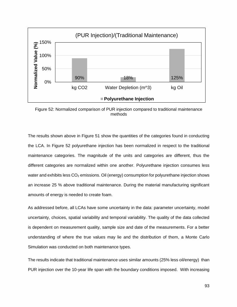
93
Figure 52: Normalized comparison of PUR injection compared to traditional maintenance methods
The results shown above in Figure 51 show the quantities of the categories found in conducting
the LCA. In Figure 52 polyurethane injection has been normalized in respect to the traditional
maintenance categories. The magnitude of the units and categories are different, thus the
different categories are normalized within one another. Polyurethane injection consumes less
water and exhibits less CO2 emissions. Oil (energy) consumption for polyurethane injection shows
an increase 25 % above traditional maintenance. During the material manufacturing significant
amounts of energy is needed to create foam.
As addressed before, all LCAs have some uncertainty in the data: parameter uncertainty, model
uncertainty, choices, spatial variability and temporal variability. The quality of the data collected
is dependent on measurement quality, sample size and date of the measurements. For a better
understanding of where the true values may lie and the distribution of them, a Monte Carlo
Simulation was conducted on both maintenance types.
The results indicate that traditional maintenance uses similar amounts (25% less oil/energy) than
PUR injection over the 10-year life span with the boundary conditions imposed. With increasing
90% 18% 125%0%
50%
100%
150%
kg CO2 Water Depletion (m^3) kg OilNo
rma
lize
d V
alu
e (
%)
(PUR Injection)/(Traditional Maintenance)
Polyurethane Injection
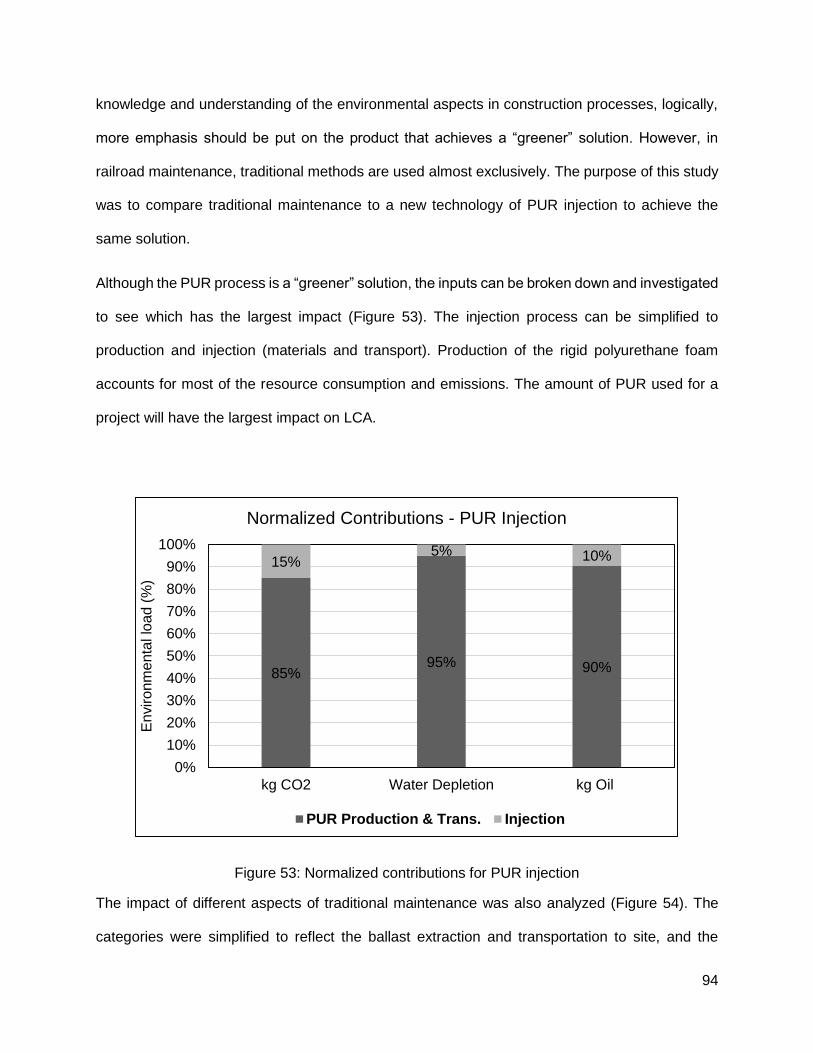
94
knowledge and understanding of the environmental aspects in construction processes, logically,
more emphasis should be put on the product that achieves a “greener” solution. However, in
railroad maintenance, traditional methods are used almost exclusively. The purpose of this study
was to compare traditional maintenance to a new technology of PUR injection to achieve the
same solution.
Although the PUR process is a “greener” solution, the inputs can be broken down and investigated
to see which has the largest impact (Figure 53). The injection process can be simplified to
production and injection (materials and transport). Production of the rigid polyurethane foam
accounts for most of the resource consumption and emissions. The amount of PUR used for a
project will have the largest impact on LCA.
Figure 53: Normalized contributions for PUR injection
The impact of different aspects of traditional maintenance was also analyzed (Figure 54). The
categories were simplified to reflect the ballast extraction and transportation to site, and the
85%95% 90%
15%5% 10%
0%
10%
20%
30%
40%
50%
60%
70%
80%
90%
100%
kg CO2 Water Depletion kg Oil
En
viro
nm
enta
l lo
ad
(%
)
Normalized Contributions - PUR Injection
PUR Production & Trans. Injection

95
maintenance equipment used to place and put the finishing surface on the track. For the
consumption of energy and emissions, the maintenance part accounts for more usage of both.
The ballast extraction technique uses water to wash the aggregate, and indicates that the ballast
aspect depletes more water.
Figure 54: Normalized contributions for traditional maintenance
Comparing traditional maintenance (ballast extraction, tamping and undercutting) to PUR
injection the main factor in polymaterials is production and transportation to the site, similar results
were found for colloidal silica and cement grouted soil barriers used (Gallagher et al. 2013). Ideally
equipment would not be mobilized a distance of 1500 km, but due to the location of the specialized
equipment, it was unavoidable. Typical mobilization distances for URETEK ICR to inject are from
80 km to 160 km (Klentzman, 2015). Depending on the transportation choice chosen in SimaPro
will change the resource consumption and emissions for mobilization of material. Material
production close to the point of mobilization will also help decrease the footprint of the activity.
71%
96%
70%
29%
4%
30%
0%
10%
20%
30%
40%
50%
60%
70%
80%
90%
100%
kg CO2 Water Depletion kg Oil
En
vir
on
me
nta
l lo
ad
(%
)
Normalized Contributions
Ballast Extraction & Trans Maintenance

96
When compared to cement and asphalt production most of the energy consumption occurs in the
manufacturing of the product. Asphalt accounts for 57% of the energy consumed (Mroueh, et al.
2001) in a construction project. PUR injection, analogous to alternative construction, uses
approximately 85% of the energy during manufacture. Bribian et al. (2010) found in the LCA
conducted for rigid polyurethane foam the global warming potential (kg CO2) was calculated to be
6.788 kg CO2/kg PUR. EPS foam has a similar global warming potential of 7.336 kg CO2. In this
study it was found to be 4.2 kg CO2/kg PUR. Polyurethane density as well as LCA temporal and
spatial variability can explain the variation of expected global warming potential. The energy
consumed while creating the PUR material in the study used 97.7 MJ/kg. In Bribian et al. (2010)
rigid polyurethane foam insulation was found to be 103.8 MJ/kg and EPS foam was 150.7 MJ/kg.
The polyurethane used in Bribian et al. (2010) was also performed for insulation panels with a
density of 30 kg/m3. Comparing PUR for injection to foams used construction materials shows
that PUR in this study is comparable (-6%) in energy usage, but for CO2 emissions, -36% less
than a comparable PUR-product.
Traditional railroad maintenance may be compared to a traditional roadway. Both systems need
quarried rock and compaction to provide a final product. The magnitudes and quantities may be
different but the general allocation of resources should be similar. For the aggregates involved in
asphalt production crushing and sieving is needed (Zapata and Gambatese, 2005). To extract,
crush, screen and transport to gate, limestone ballast requires approximately 7.76 x 10⁷
Joules/ton, where in Stipple (2001) 3.82 x 10⁷ Joules/ton was calculated. There is a factor of two
difference, but that may be an artifact of technology, location, and data. Placement energy usage
varies significantly more, but with the heavy equipment needed to tamp, place and distribute
ballast, it agrees with railroad applications requiring more energy at 8.9 x 10⁷ Joules/ton. Which
is a function of fuel consumption and production rate. Zapata and Gambatese (2005) found that
1.34 x 10⁷ Joules/ton was required to place asphalt pavement. Stripple (2001) found that for

97
crushed aggregate approximately 2.14 kg CO2 eq/kg was produced. This study conducted that
for ballast extraction 5.7 kg CO2 eq/kg was produced. There is a factor of difference of two
between Stripple (2001) and this study, data quality and temporal variability would account for
this. To analyze CO2 emissions, asphalt paving the comparable process. Over the study period
of 10-years, 7.2 kg CO2/ton is emitted from extraction and placement, Hassan (2009) found that
for hot mix asphalt 33.2 kg CO2/ton is emitted from the bitumen formation, plant operation, and
aggregates. Traditional railroad maintenance is comparable to asphalt pavement only in
aggregate production; bitumen formation and storage of the asphalt accounts for the majority of
the CO2 emissions.
PUR injection, as a maintenance strategy, avoids using traditional maintenance methods over 10-
years. During this period many products and processes are avoided, such as ballast extraction,
transportation, and tamping. The PUR injection alternative gains the benefit over 10-years of not
conducting traditional maintenance. Figure 55 shows the net benefit of PUR injection over a 10-
year period. Negative numbers indicate savings, while positive numbers indicate usage above
traditional maintenance. The manufacturing of polyurethane foam uses more energy as proven in
Figure 53.
Figure 55: Net resource usage for PUR injection
-100%
-80%
-60%
-40%
-20%
0%
20%
40%
No
rma
lize
d V
alu
e (
%)
Net Resource Usage with PUR injection
kg CO2Water Depletion (m3)
kg Oil-1608 kg
-62 m3
1146 kg

98
Significant system boundary conditions may cause much of the difference in comparable studies
(Zapata and Gambatese, 2005). Due to the lack of comparable studies, it is difficult to determine
whether the study conducted on the Dayton Dip, is representative of typical projects or only
applicable at the study site.

99
Monte Carlo Simulation
To come up with a measure of uncertainty and to determine where the range of expected values
may occur, a Monte Carlo simulation was conducted for both traditional maintenance and
polyurethane injection.
Traditional Maintenance
Uncertainty is found in all data sets especially when certain values are estimated. To estimate
traditional maintenance variation in the categories of interest, distributions of the variable were
determined through data analysis or logical bounds.
Ballast production is fairly standardized; limestone is quarried from open pits by blasting, followed
by mechanical crushing, screening, and washing to get a desired particle size distribution.
Aggregate production facilities attempt to recycle as much water as possible (~85%), but some is
lost through evaporation, wetting of aggregates and spray. A log normal distribution of the water
usage was applied to the data with a square of the standard deviation of 1.5 to introduce an
uncertainty of 50% from the average value (1 is zero uncertainty). When distributions are unknown
to an extent, but reasonably estimated, the distribution can be considered as the default
(SimaPro). Previous research in LCA distributions often find a median value then apply either a
lognormal or normal distribution with geometric standard deviation of 1.1 to 2 (Kucukvar et al.
2014; Sonneman et al. 2002).
Shipment of the ballast between quarry and project site was limited to a rectangular (bounded
uniform) distribution. The quarries in close vicinity to the Dayton Dip were approximately 4 km
and 10 km away from the selected site. Provided the quarries produce a ballast rock suitable for
track substructure, the rock would most likely come from those locations.
100
Tamping a railroad track includes production rates. A ballpark production rate was found from an
interview with a worker, which resulted in about 400 meters/hr (Tarry, 2014). During the tamping
process a typical lift of the track is limited to 50 mm per pass (Tarry, 2014). With a known site
length and a historical dip of 150 mm, as observed in the field, it would take three passes,
approximately an hour to complete the tamping of the study site. Using this time and fuel
consumption data from different Caterpillar engines employed in maintenance equipment an
average fuel consumption and distribution were established.
The railroad substructure/ballast end of life scenario was simplified, but was confirmed through
an interview with an engineer. The old ballast and substructure would be undercut and the spoils
from the event would be used to build up an embankment or flatten out slope geometry.
Polyurethane Injection
A similar approach was used to establish distributions for the resources and products used in
polyurethane injection.
Estimates from URETEK USA were used to find the average and distribution of the PUR used for
the injection. A contingency of +-10% of the estimated weight of polyurethane would be used.
Values for ±10% of the projected quantity we used to establish a uniform distribution of possible
injection. Steel rods are used to inject the PUR to the ground. A contingency of ±10% was applied
to the steel rods as well to mimic the PUR used. The PUR was assumed to be manufactured as
near as can be to the equipment that needed mobilization.
Mobilization distance was governed where the injection equipment was last used. For the study
URETEK had the equipment designed for use on railroads located around Denver, CO. To reach
the site located in Dayton, IL, there are three likely routes that will be taken: I-70, I-80, and a
combination of the two (I-80 & I-70). The distances are 1,700 km, 1,510 km and 1,710 km
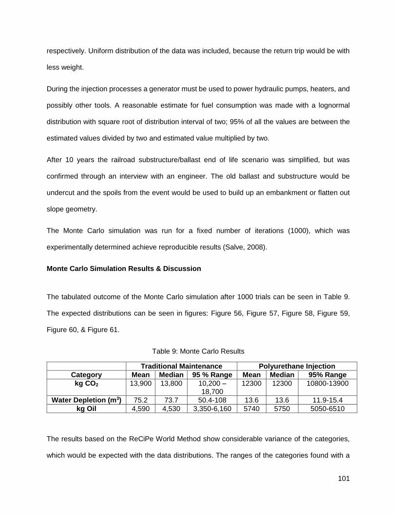
101
respectively. Uniform distribution of the data was included, because the return trip would be with
less weight.
During the injection processes a generator must be used to power hydraulic pumps, heaters, and
possibly other tools. A reasonable estimate for fuel consumption was made with a lognormal
distribution with square root of distribution interval of two; 95% of all the values are between the
estimated values divided by two and estimated value multiplied by two.
After 10 years the railroad substructure/ballast end of life scenario was simplified, but was
confirmed through an interview with an engineer. The old ballast and substructure would be
undercut and the spoils from the event would be used to build up an embankment or flatten out
slope geometry.
The Monte Carlo simulation was run for a fixed number of iterations (1000), which was
experimentally determined achieve reproducible results (Salve, 2008).
Monte Carlo Simulation Results & Discussion
The tabulated outcome of the Monte Carlo simulation after 1000 trials can be seen in Table 9.
The expected distributions can be seen in figures: Figure 56, Figure 57, Figure 58, Figure 59,
Figure 60, & Figure 61.
Table 9: Monte Carlo Results
Traditional Maintenance Polyurethane Injection
Category Mean Median 95 % Range Mean Median 95% Range
kg CO2 13,900 13,800 10,200 – 18,700
12300 12300 10800-13900
Water Depletion (m3) 75.2 73.7 50.4-108 13.6 13.6 11.9-15.4
kg Oil 4,590 4,530 3,350-6,160 5740 5750 5050-6510
The results based on the ReCiPe World Method show considerable variance of the categories,
which would be expected with the data distributions. The ranges of the categories found with a

102
95% confidence interval are logically reasonable. A few of the inputs were provided as a uniform
distribution, which equally applies probability to the whole data set. A proper determination of the
probability distribution is only possible if extensive data is available (Sonnenman et al. 2002). The
PDFs for the categories related to traditional maintenance all have a slight log normal distribution.
The resulting probablility distributions for each category of both traditional maintenance and PUR
injection show semi-symmetrical distributions. The values determined previously for the average
(mean) do not vary significantly from the mean and median calculated through the Monte Carlo
simulations. Due to the inputs for the PUR injection, the final PDFs show a more normal
distribution shape. Using a probability distribution for the input data, every category results has a
mean value and a PDF of expected values.
Categories where normal and lognormal distributions are present have the largest impact on the
outcome of the PDF shape and distribution. In the results from the Traditional maintenance,
ballast extraction and fuel consumption both had lognormal distribution applied. The effect of that
distribution is seen in the final PDF for the process. Evidence of similar distributions in the PUR
injection are seen as well, the diesel and fuel usage for injection with lognormal distributions.
Similar to Sonnemann et al. (2003) the most important parameters are the ones that impact the
PDFs most. In previous research regarding infrastructure materials a lognormal distribution with
a geometric mean of two was applied to the data, this study attempted to bound the results in an
attempt to idealize field measurements. Based on previous research, it can be determined that
material and transportation impact the results significantly for PUR injection. For traditional
maintenance the ballast extraction and movement significantly impact the result of the Monte
Carlo simulations. The uniform distribution parameters are negligible on the final PDFs of the
categories.
In a similar study by Kucukvar et al. (2014) only normal distributions were applied to asphalt
additives, transportation distance, and mixing energy. This is beneficial in providing a range in

103
which expected values may fall, but does not account for the actual distribution of the materials,
whereas in this study, ranges are bounded, and do not continue to extremely high or low values.
Uncertainties can be minimized by using specific process data for products analyzed (Kucukvar
et al. 2014). Every iteration of a risk analysis simulation must be a scenario that can occur (Walls
and Smith 1998-9). With these bounding distributions, the Monte Carlo simulation exhibits more
meaningful results.
To reiterate many studies, it is difficult to quantify uncertainty in LCA. This includes determining
the actual distribution of the data, because large quantities of data is needed for meaningful
statistics.
Improvement could be made in the LCA by conducting a traffic analysis of the spur line, to
estimate average train traffic. Foreground data regarding both the Bayer PUR product and ballast
production should be collected.

104
Figure 56: PDF for kg CO2 eq. for traditional maintenance
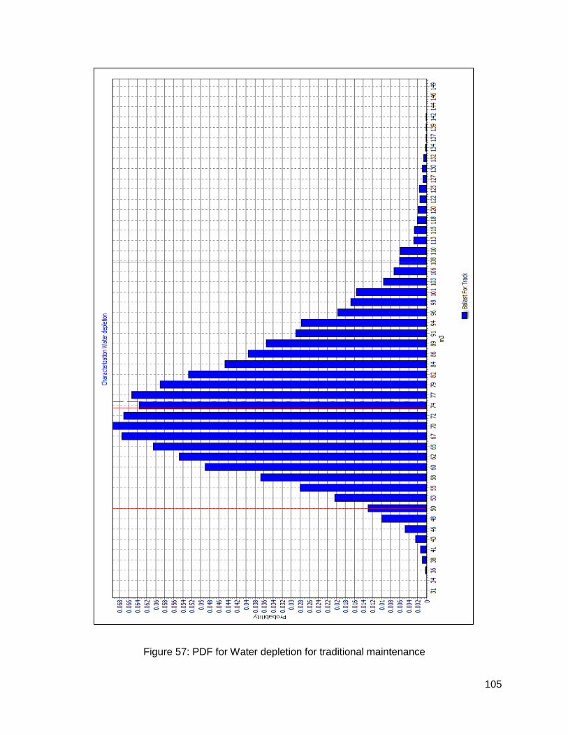
105
Figure 57: PDF for Water depletion for traditional maintenance

106
Figure 58: PDF for kg Oil for traditional maintenance

107
Figure 59: PDF for kg CO2 eq. for PUR injection

108
Figure 60: PDF for water depletion for PUR injection

109
Figure 61: PDF for kg Oil for PUR injection

110
Chapter 5: Field Injection Design and Instrumentation
Injection Strategy
The polyurethane injection strategy was designed by URETEK USA and URETEK ICR with input
from UW-Madison. Upon completion of the Geotechnical Reports, information was disseminated
to URETEK USA and URETEK ICR to complement the DCP tests. UW-Madison provided the
goals it would like to accomplish with the field site. The goals included:
1. Stabilize the subballast
2. Stabilize the subballast and subgrade soils
The two goals stated above are to investigate the effect of PUR placement throughout the
substructure of a railroad track. URETEK USA/ICR specializes in chemical grouting techniques.
As with any grouting or construction project site preparation is needed to ensure success. The
typical progression of construction includes the following steps:
1. Utilities will be marked, by the owner or an independent party
2. Additional DCP tests will be conducted to verify the length and depth of the treatable area.
This step can provide additional insight into the problem and alterations to the original plan
may be suggested. The owner must approve.
3. Hollow steel tubes/probe will be driven in the designed injection pattern. Injection of
polyurethane will be begin at this point.
4. The injections are conducted in the order of shallowest to deepest elevation.
5. Probes will be cut off at the surface.
6. Upon completion the area will be cleared of all debris and remnants.
7. Illinois Railway will level the track after injections are completed
(URETEK, 2014)

111
The goals UW-Madison designated for URETEK USA to design the injections for were to
strengthen the ballast layer and strengthen and consolidate the subgrade and subballast layer.
The overall task of strengthening and consolidating soil is typical of work URETEK conducts, but
a railroad section is unconfined. Unconfined refers to not having a sealed layer of some surface
above. HMA and PCC roads for example constitute a confined system.
The Dayton Dip has two proposed injection patterns to remediate problems and fulfill the goals
set forth. As seen in Figure 63 there are two unique plans for the Ballast Section. Two plans
provided by URETEK will be used in conjunction with a control section where no PUR will be
placed. The sections will be approximately 25 m long. The first injection pattern will be stabilize
the subgrade and subballast. The DCP results showed low penetration indices in the ballast,
although the ballast is highly fouled, the subballast and subgrade layers of this section were weak.
This weakness will be remediated by chemical compaction grouting. The material once injected,
expands in a bulb type shape and increases confinement on the adjacent soil. This may compact
coarser grain soils (densify) and consolidate fine grained soils. The same technique will be used
in the second proposed section, along with reinforcing the subballast below the ties. To prove
multiple years of research at UW-Madison (Keene, 2012; Dolcek, 2014) which utilized clean and
fouled ballast with PUR reinforcement under cyclic loading, this injection type will serve as a field
verification.
The bridge approach will receive a similar treatment with chemical compaction grouting and
permeation grouting. The compaction grouting will occur in the fine grain subgrade soils, and the
permeation grouting will be conducted 0.5 m below the track surface. The stepped injection
method seen in Figure 64 creates a stepped stiffness transition. This stepped stiffness transition
eases the changing stiffness’s from the bridge to the ballasted track. Previous researchers have
used rubber pads, wooden ties instead of concrete, and plastic ties to achieve this same transition
(Mishra et al. 2012). The compaction grouting should stiffen the subgrade layer which has been

112
shown to be the deleterious part of the track embankment. This should coincide with findings from
Li and Davis (2005) where remedial measures in the subgrade layer are ineffective if they do not
produce a consistent and acceptable track stiffness between the ballasted track and bridge.
Field Injection Methodology
Low-quality track might support relatively high axle loads with a high-maintenance regime;
conversely, higher investment can mean higher axle loads and relatively low maintenance
Australian Government (2003). This methodology is applicable to both monetary investment and
time required to maintain track. PUR injection may be a higher maintenance investment upfront,
but should prove to be a useful tool that can be used for maintenance.
HMA layer model
Previous research conducted by Keene (2012) outlined two procedures that could be potentially
used in the field for stabilization and improvement of the ballast layer. One strategy was similar
to that of an HMA layer used as a subballast. Installing an HMA base for a railroad track requires
significant amount of work, essentially new construction. If the layer is installed correctly, and
does not fail, it is an effective method or reducing the stress to the subgrade. It also sheds water
from the rain, not allowing infiltration into the subgrade beneath the track. The ability to install
PUR at a depth and thickness similar to a HMA layer will provide the benefits of an HMA layer
without the reconstruction process.
Compaction grouting
The use of cementitious grouts to improve soil characteristics is not a novel concept. Grouting is
an injection of fluid, typically cement based, into a soil column to fill fissures, cracks or void
(Houlsby, 1990).

113
Figure 62: Compaction grouting (skanska.co.uk)
Grout can also be injected at a pressure high enough to displace soil and compact the soil
structure, this is referred to low mobility or compaction grouting. Low mobility grout does not travel
along the fissures or cracks, but remains localized to the injection area (Brill and Hussin, 1992).
This allows a high pressure to be applied to provide compaction/compression to the surrounding
soils (Figure 62). The impact on both coarse and fine grained soils consists of a higher density
and stiffness as well as a column of grout to increase local bearing capacity (Brill and Hussin,
1992; El-Kelesh et al. 2012).
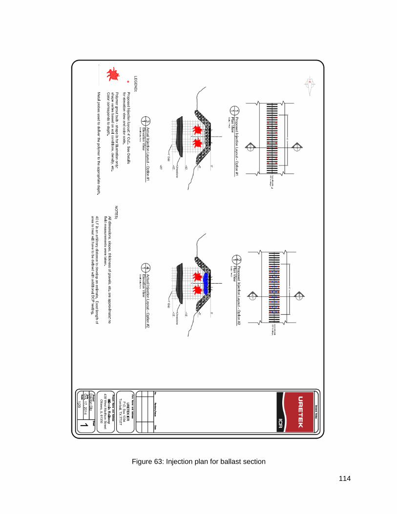
114
Figure 63: Injection plan for ballast section

115
Figure 64: Injection plan for bridge approach

116
Instrumentation
To determine whether the PUR injections have been successful a metric and measurement
techniques shall be employed. The measurements will be short term (dynamic), and long term
(settlement). Monitoring both of these responses should provide insight whether the PUR injection
has benefitted the railroad track section.
To monitor short term settlement Fiber Optic Strain gauges (FOS) will be used. FOS can detect
and distinguish both lateral and normal strains in railway infrastructure applications without direct
use of track vehicles. In addition to being non-intrusive and convenient, there are several
advantages to the use of FOS in railway inspection, including lasting durability, high deformation
range, high temperature endurance, immunity to electromagnetic noise, electrical isolation,
distributed sensing capability, multiple sensing capabilities, and the potential for relatively low cost
when applied to large distance distributed monitoring of structures (Alsabhan, 2013). Micron
Optics OS3155 sensors were chosen for the monitoring. These sensors contain temperature
compensating Fiber Bragg Grating.
One of the key causes for maintenance events is deformation of the superstructure.
Superstructure deformation often comes from the substructure, where ballast and subgrade soils
often are the reason for the deformation. Speed limitations, ride comfort, and track stability are
indicators of maintenance. They superstructure can be monitored to provide an idea of how much
settlement the substructure is undergoing. Without discrete settlement measurements, discerning
where the largest deformations are occurring is difficult. From the GPR results, there are two main
unique layers: ballast/fouled ballast and the subgrade. Monitoring these two discrete soil layers
provides insight into the weaker of the two.
To monitor the ballast, survey reflectors will be placed every 2 m on the rail web. The reflectors
were placed on both rails to provide information on differential settlement and heterogeneities in

117
the injection process. To isolate the ballast layer 6 settlement rods will be installed in the three
unique sections. The settlement rods were installed at the interface between the subballast and
the subgrade layer similar to Mishra et al. (2012).

118
Chapter 6
Concluding Remarks
The background information, previous research and site investigations have resulted in selecting
the bridge approach as the PUR injection area. The impact of remediating the rail road bridge
approach may have a broader impact on the rail transit community. Railroad embankment fills
and the native soil the embankments are constructed on are occasionally not ideal for increased
cyclic stress from rail traffic. The geotechnical and geophysical results indicate at the points of
highest stress, transition zones, subgrade soil is failing. The failure zone is reflected in the
subballast and ballast layers and additional aggregate is added to keep the track level.
Remediation of the subgrade failure is completed by the UDI method, targeting soft zones of
subgrade. Changing foundation stiffness from one track structure to another (ballasted track to
timber bridge) can cause large dynamic loads (Nicks, 2009). The stepped elevation method of
the UDI parallel with the track should decrease the abrupt stiffness change to the bridge, similar
to what is done with plastic ties or rubber rail seat pads.
The LCCA and LCA were conducted on the Ballast section for multiple reasons. First, boundary
conditions, it is more reasonable to establish boundary conditions on a simple tangent track. The
other reason was for these studies to be valid, the methods of maintenance have to be similar.
The stepped UDI method used at the approach may solve multiple problems other than soft
subgrade soils. In order to have comparable results the targeted problem should be solvable by
both methods. Both the LCA and LCCA indicated that within the time line and boundary conditions
that PUR injection, if successful, is a valuable solution for poor subgrade and ballast conditions.
As additional information is gathered from the field study, curious individuals should contact
119
Chapter 7: References
Abdelhalim, B., Kirkham, R., (2004). Whole Life-Cycle Costing. Oxford. Blackwell Publishing
Ltd.
Alsabhan, A. (2013). “Warning systems and inspection for maintenance of freight railways.” MS
Thesis. Department of Civil and Environmental Engineering, University of Wisconsin-Madison.
Alsabhan, A. (2015). “GPR and TDR results for the Dayton Dip.” Department of Civil and
Environmental Engineering, University of Wisconsin-Madison. Internal memo.
Amtrack Office of Inspector General. Retrieved from
http://www.amtrakoig.gov/sites/default/files/reports/EVALUATIONREPORT-92809.pdf
Anders, E., & Bjorn, P. (n.d.). Executive summary of the concluding technical repory. Retrieved
April 23, 2015, from
http://www.voestalpine.com/schienen/static/sites/c011/downloads/downloads/INNOTRACK_-
_Summary_and_highlights.pdf
Anderson, W.F. & Fair, P. (2008). “Behavior of Railroad Ballast under Monotonic and Cyclic
Loading.” Journal of Geotechnical and Geoenvironmental Engineering, ASCE, 134(3), 316–328.
Ashby, M. (1983). The mechanical properties of cellular solids. The Metallurgical Society of
AME, 14A, 1755-1769.
Aursudkij, A., McDowell, G.R., Collop, A.C. (2009). “Cyclic Loading of Railway Ballast Under
Triaxial Conditions and In A Railway Test Facility.” Granular Matter, (11), 391–401.
Ayers, M., Thompson, M. Uzarksi, D. (1989) Rapid Shear strength evaluation of in situ granular
materials. Transportation Research Board. June 1990, 1227, 143-146.
Baumann, Heike, and Anne-Marie Tillman. (2004). The Hitch Hiker’s Guide to LCA. Lund:
Studentlitteratur, AB.
Bayer Material Science (2010). 486STAR Polyurethane Foam Grout. Technical Data Sheet,
Spring, Texas.
Beals, J.T., & Thompson, M.S. (1997). Density gradient effects on aluminium foam compression
behavior. J Mater Sci., 32 (1997), pp. 3595–3606
Boler, H. (2012). "On the Shear Strength of Polyurethane Coated Railroad Ballast." MS Thesis,
Department of Civil and Environmental Engineering, University of Illinois at Urbana-
Champagne.
Bribián, I., Capilla, A., & Usón, A. (2010). Life cycle assessment of building materials:
Comparative analysis of energy and environmental impacts and evaluation of the eco-efficiency
improvement potential. Building and Environment, 1133-1140.
Bribián, I., Capilla, A., & Usón, A. (2010). Life cycle assessment of building materials:
Comparative analysis of energy and environmental impacts and evaluation of the eco-efficiency
improvement potential. Building and Environment, 1133-1140.
120
Brill, G.T. Hussin, J.D. (1992) The use of compaction grouting to remediate a railroad
embankment in a karst environment. In-situ soil modification. Louisville, Kentucky.
Byun, Y., Kim, J., & Lee, J. (2013). Cone Penetrometer with a Helical-Type Outer Screw Rod for
Evaluation of the Subgrade Condition. Journal of Transportation Engineering, 115-122.
Casagrande, A. (1931) Discussion of frost heaving. Highway Research Board, Proceeding, V. II.
168-172.
Chan, A., Keoleian, G., & Gabler, E. (2008). Evaluation of Life-Cycle Cost Analysis Practices
Used by the Michigan Department of Transportation. Journal of Transportation Engineering,
236-236.Evaluation Report E-09-05 Amtrack's Infrastructure Maintenance Program. (2009).
Dolcek, T. (2013). “Mechanical Behavior of Polyurethane Stabilized Fouled Ballast (PSFB).” MS
Thesis. Department of Civil and Environmental Engineering, University of Wisconsin-Madison.
Ebrahimi, A. & Keene, A.K. (2011). "Maintenance Planning of Railway Ballast." AREMA 2011
Annual Conference, Minneapolis, Minnesota, September 18-22.
Ebrahimi, A. (2011). “Deformational Behavior of Fouled Railway Ballast.” PhD thesis,
Department of Civil and Environmental Engineering, University of Wisconsin, Madison.
El-Kelesh, A., Matsui, T., & Tokida, K. (2012). Field Investigation into Effectiveness of
Compaction Grouting. Journal of Geotechnical and Geoenvironmental Engineering.
Esveld, C. (1990). Computer-aided maintenance and renewal of track. Railroad Conference,
1990, Technical Papers Presented at the 1990 ASME/IEEE Joint, pp.165-170.
Fluet, J. (1986). Geosynthetics and North American railroads. Geotextiles and Geomembranes.
201-218
Frohling, R. D., Sheffel, H., and Ebersohn, W. (1995). “The vertical dynamic response of a rail
vehicle caused by track stiffness variations along the track.”Proc., 14th IAVSD Symp.,
International Association for Vechicle System Dynamics, Praha, Czech Republic.
Gallagher, P., Spatari, S., & Cucura, J. (2013). Hybrid life cycle assessment comparison of
colloidal silica and cement grouted soil barrier remediation technologies. Journal of Hazardous
Materials, 421-430
Glick, S. (2007). Life-cycle assessment and life-cycle costs: A framework with case study
implementation focusing on residential heating systems
Goering, D. (2003). ”Passively Cooled Railway Embankments for Use in Permafrost Areas.”
Journal of Cold Regions Engineering, 17(3), 119–133.
Guangli Du & Raid Karoumi (2013): Life cycle assessment of a railway bridge: comparison of
two superstructure designs, Structure and Infrastructure Engineering: Maintenance,
Management, LifeCycle Design and Performance, volume 9, Issue 11.
Guangli Du & Raid Karoumi, Structure and Infrastructure Engineering (2012): Life cycle
assessment framework for railway bridges: literature survey and critical issues, Structure and

121
Infrastructure Engineering, Life-Cycle Design and Performance, Ahead-of Print, DOI:
10.1080/15732479.2012.749289
Hakan Stripple and Stefan Uppenberg. (2010) Life cycle assessment of railways and rail
transports – Application in environmental product declarations (EPDs) for the Bothnia Line. IVL
Swedish Environmental Research Institute. Ltd.
Hassan M. Life-Cycle Assessment of Warm-Mix Asphalt: an environmental and economic
perspective. In: Proceedings of 88th transportation research board annual meeting. Washington
D.C., USA; 2009. p. 1–15.
Hay, W. (1982). Railroad engineering (2nd ed.). New York: Wiley.
Hendrickson, C., & Horvath, A. (2000). Resource Use and Environmental Emissions of U.S.
Construction Sectors. Journal of Construction Engineering and Management, 38-44.
Hesse, D. (2013). “Impact of Increasing Freight Loads on Rail Infrastructure from Fracking Sand
Transport.” MS thesis, Department of Civil and Environmental Engineering, University of
Wisconsin-Madison.
Hesse, D. Tinjum, J.M., Warren, B.J. (2014). Impact of increasing freight loads on rail
substructure from fracking sand transport. Transportation Geotechnics. doi:
http://dx.doi.org/10.1016/j.trgeo.2014.06.003
Heydinger, A. G., Xie, Q. L., Randolph, B. W. and Gupta, J. D. (1996). “Analysis of Resilient
Modulus od dense and Open-graded Aggregates.” Transportation Research Board,
Washington, D.C., No.1547, 1-6.
Houlsby AC. (1990) Construction and design of cement grouting. In: A guide to grouting in rock
foundations. New York: John Wiley and Sons.
Sophia Lisbeth, H. (2010). Life Cycle Assessment of Materials and Construction in Commercial
Structures : Variability and Limitations. Masters Thesis, MASSACHUSETTS INSTITUTE OF
TECHNOLOGY.
Indraratna, B., Rujikiatkamjorn, C.. Chu, J. (2007). Soft clay stabilization with Geosynthetic
Vertical drains beneath road and railway embankments: A critical Review of analytical solutions
and numerical analysis. Colorado ASCE Special Publication.
Indraratna, B., Numbalkar, S., Shrawan, S. (2013) The role of geosynthetics in improving the
behavior of ballasted rail tracks. In G. Venkatappa Rao (eds.). Geosynthetics in railway track.
Centrail Board of Irrigation and Power. India. (59-85)
Indraratna, B., Nimbalkar, S. & Rujikiatkamjorn, C. (2012). Stabilising railway embankments with
geosynthetic grids and drains and a class A prediction of track behaviour. International
Symposium on Sustainable Geosynthetics and Green Technology for Climate Change (SGCC)
(pp. 21-40).
Indraratna, B., Salim, W., and Rujikiatkamjorn, C. (2011).Advanced rail geotechnology:
Ballasted track, CRC Press/Balkema, Rotterdam, Netherland
-- Life cycle assessment -- Principles and
framework. (2006).

122
ISSMFE TC-8 (1989) “Grain size distribution as a frost susceptibility criterion of soil,” VTT
Symposium, vol. 1, pp.29-32.
Keene, A. (2012). “Mitigating Ballast Fouling Impact and Enhancing Rail Freight Capactiy.”MS
Thesis. Department of Civil and Environmental Engineering, University of Wisconsin-Madison.
Kerr, A. D., and Bathurst, L. A. (2000). “Pads ease track transitions.”Railw. Track Struct.,
August, 57–64.
Kerr, A. D., and Moroney, B. E. (1993). “Track transition problems and remedies.” Bulletin 742,
American Railway Engineering Association, Landover, Md., 267–298
Koerner, R. (1998) Designing with Geosynthetics (4th ed.) Prentice Hall
Kramer, S. (1996) Geotechnical Earthquake Engineering. Prentice Hall
Kecukvar, M., Noori, M., Egilmez, G., & Tatari, O. (2014). Stochastic decision modeling for
sustainable pavement designs. Int J Life Cycle Assess.
Klentzman, R. "URETEK mobilization distances." Message to Benjamin Warren. (May 12th,
2015). E-mail.
LaGrega MD, Buckingham PL, Evans JC. (1994). Hazardous Waste. 761 Management. New
York: McGraw-Hill.
Lekarp, F., Isacsson, U. and Dawson, A. (2000). “State of the Art.II: Premanent Strain
Response of Unbound Aggregates.” Journal of Transportation Engineernig , No.126,
Washington, D.C., 76-83.
Life cycle management for railway bridge assets Proceedings of the Institution of Mechanical
Engineers, Part F: Journal of Rail and Rapid Transit September 2013 227: 570-581,
doi:10.1177/0954409713501297
Lioyd, D.J. (1994). Particle reinforced aluminium and magnesium matrix composites. Inter Mater
Rev., 39 (1) pp. 1–23
Menges, G., & Knipschild, F. (1975). Estimation of mechanical properties for rigid polyurethane
foams. Polymer Engineering and Science, 623-627.
Mishra, D., Tutumluer, E., Stark, T., Hyslip, J., Chrismer, S., & Tomas, M. (2012). Investigation
of differential movement at railroad bridge approaches through geotechnical instrumentation.
Journal of Zhejiang University SCIENCE A, 814-824
Marsh, B. & Schaalma, R, "WSOR Maintenance Information." Message to Benjamin Warren.
(January 28th, 2015 to February 6th, 2015). E-mail.
Mitchell, J.K. 1993. Fundamentals of soil behavior. John Wiley & Sons, Inc., N.Y.
Moy, P., Clark, G., Hart, D., Mickelsen, D., Luloff, A., Angel, K., Barrett, K., & Wu , C. Boldt, S.
(2011). Climate change and wisconsin's great lakes coastal communities. Wisconsin's Changing
Climate: Impacts and Adaptation. Costal Communities Working Group.
Mroueh, U., Eskola, P., & Laine-Ylijoki, J. (2001). Life-cycle impacts of the use of industrial by-
products in road and earth construction. Waste Management, 21(3), 271-277.

123
Nielsen, D., Raman, D., Chattopadhyay, G. (2013). Life cycle management for railway bridge
assets. Proceedings of the Institution of Mechanical Engineers Part F-Journal of Rail and Rapid
Transit 09/2013; 227(5):570-581. DOI:10.1177/0954409713501297
Nicks, Jennifer Elizabeth (2009). The Bump at the End of the Railway Bridge. Doctoral
dissertation, Texas A&M University. Available electronically from http : / /hdl .handle .net /1969
.1 /ETD -TAMU -2009 -12 -7432.
Nurmikolu, A. (2005). Degradation and Frost Susceptibility of Crushed Rock Aggregates Used
in Structural Layers of Railway Track. PhD Dissertation, Tampere University of Technology.
Pan, T., Tutumluer, E. and Anochie-Boateng, J. (2006). “Aggregate Morphology Affecting
Resilient Behavior of Unbound Granular Materials.’ Trasnportation Research Record: Journal of
the Transportation Research Board, No.1952, Washington, D.C., 12-20.
Paulsson, B., & Ekberg, A. (2010). Cutting the life-cycle cost of track. Railway Gazette
International, 166(1), 48-52.
Priest, J., & Powrie, W. (2009). Determination of Dynamic Track Modulus from Measurement of
Track Velocity during Train Passage. Journal of Geotechnical and Geoenvironmental
Engineering, 1732-1732.
Pucci, M.J. (2010). “Development of a Multi-Measurement Confined Free-Free Resonant
Column Device and Initial Studies.” MS thesis, Department of Civil, Architectural and
Environmental Engineering, University of Texas, Austin.
Raymond, G.P., 2002, "Reinforced Ballast Behaviour subjected to Repeated Load", Geotextiles
and Geomembranes, Vol. 20, pp. 39 - 61.
Rosa, M. (2006). “Effect of Freeze and Thaw Cycling on Soils Stabilized using Fly Ash,” MS
Thesis. University of Wisconsin-Madison, Madison, WI.
Rose, J., Brown, E., & Osborne, M. (2000). Asphalt Trackbed Technology Development: The
First 20 Years. Transportation Research Record, 1-9.
Salve, J.L. (2008). “Dealing with uncertainties in Life Cycle Assessment for emerging
technologies.” MS Thesis, School of Science, Open University of the Netherlands.
Santamarina, J.C. and Cho, G.C. (2004), Soil Behavior: The Role of Particle Shape, Proc.
Skempton Conf., March, London.
Simonsen, E., & Isacsson, U. (1999). Thaw weakening of pavement structures in cold regions.
Cold Regions Science and Technology, 29, 135-151.
Stripple, H. (2001). Life cycle analysis of road; A pilot study for inventory analysis, Swedish
Environmental Research Institute (IVL), Gothenburg, Sweden.
Su, Z., Fratta, D., Tinjum, J., & Edil, T. (2013). CEMENTITIOUSLY STABI LIZED MATERIALS
USIN G ULTRASONIC TESTING. TRB 2013 Annual Meeting. Retrieved April 23, 2015.
Szycher, M. (1999). Szycher's handbook of polyurethanes. Boca Raton: CRC Press.

124
Table 4-17: Class I Rail Freight Fuel Consumption and Travel | Bureau of Transportation
Statistics. (n.d.). Retrieved April 23, 2015, from
http://www.rita.dot.gov/bts/sites/rita.dot.gov.bts/files/publications/national_transportation_statisti
cs/html/table_04_17.html
Tarry, P. (2014) “ How the track tamping machine is used.” Response to comments.
www.evra.org.uk/engineering/How%20the%20tamper%20works.doc
Tian, P., Zaman, M. M. and Laguros, J. G. (1998). “Gradation and Moisture Effects on Resilient
Moduli of Aggregate Bases.” Transportation Research Record, No.1619, Washington, D.C., 75-
84.
Toros, U. & Hiltunen., D.R. (2008). “Effects of Moisture and Time on Stiffness of Unbound
Aggregate Base Course Materials.” Transportation Research Record, No. 2059, Washington,
D.C., 41–51.
Vanapalli, S.K., Fredlund, D.G., Pufahl, D.E., and Clifton, A.W. 1996, Model for the Prediction of
Shear Strength with Respect to Soil Suction, Can. Geotech. J., 33, pp.379–392.
Walls, J., & Smith, M. (1998-9). LIFE-CYCLE COST ANALYSIS IN PAVEMENT DESIGN -
INTERIM TECHNICAL BULLETIN. Federal Highway Administration
Warren, B. (2014). “PUR bonding in relation to grain size.” Internal Memo. Department of Civil
and Environmental Engineering, University of Wisconsin-Madison.
Webb, G., Webb, D., Zarembski, A.M., Gauntt, J.C., and Corallo, D.L. (2012) “Tie Guide”.
Fayetteville, GA.
Wu, Y., Parker, F. and Kandhal, P. S. (1998). “Aggregate Toughness/Abrasion Resistance and
Durability/Soundness Tests Related to Aspahlt Concrete Performance in Pavements.”
Transportation Research Record, No.1638, Washington, D.C., 85-93.
Yarbasi, N., Kalkan, E., & Akbulut, S. (2007). Modification of the geotechnical properties, as
influence by freeze-thaw, of granular soils with waste additives. Cold Regions Science and
Technology, 48, 44-54.
Zapata, P., & Gambatese, J. (2005). Energy Consumption of Asphalt and Reinforced Concrete
Pavement Materials and Construction. Journal of Infrastructure Systems, 11(1), 9-20.

125
Appendix A
Freeze-Thaw Cycling
Seasonal variation in temperature and moisture in soils occur most places across the United
States. In northern climates there are periods where soils are subjected to multiple freeze thaw
cycles in a single season. Quantifying the number and effect of freeze thaw cycles is essential to
the design of long lasting transportation infrastructure. With potential increase of freeze thaw
cycles in Wisconsin there is cause for concern about how geological materials will behave (Moy
et al. 2011).
There has been investigation into roadway materials and the effect of F-T. Surface layers, base
course material, and subgrade soils have been investigated for the effect of F-T action Rosa
(2006); Simonsen and Isacsson (1999); Yarbasi et al. (2007).
In railway infrastructure there is even more cause for concern with F-T action. Railway
embankments are exceptionally susceptible to thaw settlement Goering (2003). Due to the
necessary precise positioning of the rails there is a need to maintain the alignment for train
passage during these times. Similarly, these effects occur in roadways, where frost action causes
roads to heave, settle and decrease in performance (Simonsen and Isacsson, 1999).
From groundwork laid by Casagrande (1932) there is cause to believe that fouled ballast will be
susceptible to frost action. From ISSMFE (1989) there are three criteria that must be meet for a
soil to be classified as non-frost susceptible which are:
1) Soil contains ≤ 1% of < 0.002 mm grain size material
2) Soil contains ≤ 3% of < 0.02 mm grain size material
3) Soil contains ≤8% of < 0.074 mm grain size material

126
In areas where subgrade pumping occurs or there is a large supply of windblown material,
particles that fulfill this criteria can be present in the quantities that cause frost susceptibility.
Regions where clay subgrade is present, pumping can occurring causing these particles to
infiltrate the ballast layer.
The encapsulation of the ballast, fouling and water can be idealized as a mass of low hydraulic
conductivity media. Situations where a low hydraulic conductivity media located beyond the
effects of the peizometric surface can be modeled as a closed system Simonsen and Isacsson
(1999). Closed systems operate independent of the water table and the residual water content is
the only water available for freezing action.
Laboratory investigations into freeze-thaw and frost susceptibility of ballast have been conducted
previously Nurmikolu (2005).
ASTM D5918 suggests that 1-D freezing should be done on soil samples when interests in
heaving and consolidation are of interest. One dimensional freezing is done by placing hollow
plates that circulate fluid that is causes a thermal gradient within the sample resulting in eventual
freezing. Freezing a specimen in the way, is similar to what occurs in a road bed. Rosa (2006)
investigated whether there was a difference in response of samples frozen in 1-D or 3-D. Rosa
(2006) determined that 1-D freezing takes a longer time, and no difference in trends of resilient
modulus or unconfined compressive strength were present when samples were frozen in 3-D.
Railway embankments are typically 0.5 m above the surrounding surface. Freezing in 3-D may
represent a railway embankment better than what 1-D freezing may do.
Standards of testing and quantifying the effects of F-T (ASTM D6035/D560) have been
established for granular material, and cemintitously stabilized soils. Yarbasi et al. (2007) used F-
T in conjunction with non-destructive testing, and destructive testing to quantify the effects of F-T
127
on fly ash, lime, and red-mud cement additives in granular soils. Su et al. (2013) used ultrasonic
pulse velocity measurements to quantify F-T effects on nine cementitiously stabilized mixtures.
Using a procedure shown in Keene (2012) for using p-wave velocity to track damage along with
cyclic triaxial testing was chosen for these samples.
Freeze Thaw Cycling
In order to quantify the effect of F-T action on PSFB, specimens were subjected to multiple sets
of F-T cycles. Unsure on the effect of the expansion and contraction of the water in the matrix of
fouling, ballast and RPF, after the F-T cycles were completed cyclic triaxial testing would be
conducted.
Initially, the specimens were subjected to a cyclic triaxial test (σd=350 kPa, σ3=100 kPa) for
200,000 cycles. Upon completion a constrained modulus test was conducted to track damage,
and to acquire a baseline from which the constrained modulus during the F-T cycles would be
compared to. Due to the large sample size traditional standards for freeze-thaw were not sufficient
so modifications were done.
PSFB specimens were sealed with plastic sheeting to prevent water loss during the F-T cycles.
Referencing ASTM D6035 and D560 weights and heights were tracked throughout the cycles. A
freezing-point test could not be conducted on the ballast and RPF, therefore the method to freeze
the samples was determined through Rosa (2006). Rosa (2006) determined there was no
difference between 1-D and 3-D freezing when testing for mechanical behavior. Three
dimensional freezing was chosen at a temperature of -22°C, to fulfill Rosa (2006) and ASTM
D6035/D560.
ASTM D6035 specifies a method to determine the effect of freeze thaw impacts on hydraulic
conductivity. Specifications were used from this to determine the guidelines to conduct the cycling
of the specimens. The large sample size of the PSFB required that addition time was required to
128
freeze and then thaw the sample. A hole was drilled at the midpoint of the sample, to the center,
and a thermocouple was installed. Insulating material was placed in the hole to isolate the
thermocouple from outside effects. Temperature was logged for a F-T cycle to determine the
required timing. It took approximately 32 hours to freeze or thaw the sample. For ease of sample
changing F-T cycles was 96 hours ( F-48 hr, T-48 hr). In the Figure 65, below, displays the
temperature from an instrumented sample. Room temperature was approximately 22 °C to 23 °C
during the thaw cycle.
Figure 65: Freeze and thaw timing
To track internal damage occurring in the PSFB specimens, without further damage, constrained
modulus tests were conducted at 5, 10, and 20 cycles. The tests were conducted once the
samples were thawed. Once 20 F-T cycles were achieved another cyclic triaxial test was
conducted to determine the effects on mechanical behavior.

129
Results
Freeze-thaw Testing
Over the 20 designated freeze-thaw cycles physical and mechanical properties were measured
to determine if any deterioration was occurring. During each cycle when rotating specimens,
masses and dimensions were noted. In addition to the physical measurements of the specimens
non-destructive dynamic testing was conducted after 5, 10, and 20 cycles.
Weights and Dimensions
Figure 66: Freeze Thaw Weight Tracking
In Figure 66, seen above there was little deviation from the initial weights. The specimens were
wrapped and sealed in plastic to prevent weight change. Some of the discrepancies are related
to the scale used to measure, as the resolution and accuracy were questionable, but provided
repeatable results. Unknown at the time, the scale being used for the first 6 cycles was quite
inaccurate, and results from this period should be taken lightly. The other local spikes during the
measurements relate to when laboratory humidity was higher than usual, and condensation
occurred very rapidly on the cold samples (-23 ºC).

130
Dimension Change
Two dimensions of the specimens used for F-T testing were measured concurrently with the
weights. Measurements of the height and circumference were taken after each F-T cycle to the
nearest millimeter. Height was measured at two points on the sample, where circumference was
measured at three points. The measurements were averaged after each cycle and can be seen
in Figure 67 & Figure 68.
Figure 67: F-T Height Tracking
Figure 68: F-T Circumference Tracking

131
The samples were designed to have a 798 mm circumference (127.5 mm radius). The samples
were all extremely close to this designed value, but were not exact. The concern is the change
from the initial measurement, but as seen in Figure 67 and Figure 68 there was no noticeable
change of dimension during freeze thaw.
Non-Destructive Testing
To see if any internal damage or degradation was occurring due to the F-T cycles. Prior to
subjecting the specimens to F-T testing a non-destructive test was used to find the constrained
modulus, which will now be referred to as seismic testing. The constrained modulus indicates
whether there is internal degradation occurring in the specimens. With internal degradation, one
expects ballast-to-ballast contacts to be less intact and the PUR restraining movement of the
ballast and fouling may degrade as well. Water present in the sample also may exert a
deteriorative force on the ballast and PUR. The fouling material contains 8% to 24% water by
mass. Water expands by approximately 9% by volume when the transition is made from the liquid
to soild state.
In the figures below is the constrained modulus at 30 kPa confining pressure. Tests were
conducted at 10 kPa and 20 kPa, but the data at 30 kPa had much less variance than the other
confining pressures. 30 kPa provides a better bond between the end caps and the sample, which
attributes to cleaner data and less noise.
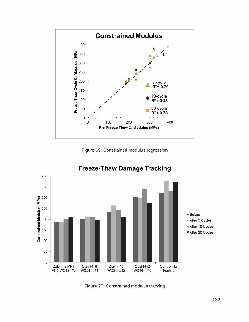
132
Figure 69: Constrained modulus regression
Figure 70: Constrained modulus tracking
133
The constrained modulus was determined before any F-T tests and is shown as the x-axis of
Figure 69. The 1:1 line on Figure 69, is the pre-F-T constrained modulus plotted against itself. A
simple linear regression was conducted from this 1:1 (pre-F-T) line. The 5-cycle constrained
modulus varies from the 1:1 line, but not by a significant amount (R2 = 0.79). Similar results are
seen after the completion of 10 cycles (R2 = 0.88) and 20 cycles (R2 = 0.78).
Some variation is seen between testing intervals (Figure 69 & Figure 70). No observable trends
are found either. The largest difference in measurements (10 to 20 cycle) was 65 MPa in the Coal
FI12 WC14 sample. Density did not change throughout the process, but for a change in
constrained modulus of 65 MPa, a variation in velocity of 8 m/s is needed. The variation may be
due to testing method errors, specifically the gauge used to apply confining pressure has limited
resolution.
Cyclic Triaxial
To adequately quantify whether F-T cycles impact the performance of PSFB specimens at sub-
saturated water contents cyclic triaxial testing was conducted after the 20 F-T cycles. Prior to the
F-T cycling specimens were subjected to 200,000 loading cycles at 350 kPa. This is designated
as cycles 1 – 200,000 in Figure 71 below. From 200,000 to 400,000 the behavior after F-T is
captured.

134
Figure 71: Cyclic triaxial results for F-T specimens

135
PUR Water Absorbance
The water absorbance of closed cell rigid polyurethane foam is typically governed by the density
of the foam (Szycher, 1999). Figure 72 below is from Szycher (1999) the relations shown are
directly related to the achieved density of the foam. The foam used in this study (URETEK
486STAR-4 BD) was typically in the range of 70 kg/m3 to 90 kg/m3 (4.36-5.61 lb/ft3). This range is
on the high end of the spectrum, but there is expected to be high strength and low water
absorbance.
Figure 72: Cellular foam density and strength (Szycher, 1999)
Water is found everywhere in a rail cross section: the substructure through capillary action, fouling
material and potentially a high water table submerging the soils. The effect of water on soils,
ballast and a combination of them (fouling) have been examined by previous researchers
Ebrahimi (2011); Keene (2012); Hesse (2013).

136
Ballast, subballast, and subgrade, experience numerous wetting and drying cycles throughout
their lifetime. These wet/dry cycles are mostly caused from influxes in precipitation, but can also
stem from other sources such as water table increases and flooding. Material and aggregates
used in construction should be weather resistant so they do not degrade and breakdown when
subjected to wetting and drying (Wu et al. 1998). For PUR to be used in construction as a weather
resistant material, it should display characteristics similar to those of aggregate: robust and
weather resistant to wetting.
Methods and Materials
The PUR foam used in this micro-study was URETEK 486STAR-4 BD which was injected into a
150 mm diameter PVC pipe, which had an approximate 10 kg weight applied to the surface to
prevent free rise of the foam. After 24 hours the foam was removed from the mold and sectioned
into appropriate specimen sizes by a corer and band saw. The dimensions of the specimens were
governed from ASTM D2166.
The test specimens were placed in a sealed vessel which had a purge valve installed to eliminate
all trapped air during filling. De-ionized water was used to fill the vessel and submerge the
specimens. Once filled and all air evacuated, every 48 hours the vessel was rotated and disturbed
to ensure all sides of the PUR specimens were exposed equally to the water.
After 120 days the samples were removed and analyzed by BS 12087-1997 (Thermal insulating
products for building applications – Determination of long term water absorption by immersion.
Method 2A was chosen from BS 12087-1997 for the simplicity and method 1B not being
conducted. The results are seen in Table 10.

137
Results
Table 10: Water absorbance
Sample Number Method 2A L.T. Absorption
(BS 12087)
Sample 05 4.08%
Sample 10 4.07%
Sample 14 3.13%
Sample 19 3.05%
Sample 01 2.92%
Sample 02 3.01%
Average 3.38%
Besides the absorption of the material, dimensions were measured before and after the
absorption test to determine physical changes. For all samples there was there was an average
swell of approximately 1 mm3, which could readily be influenced by error using Fournier calipers.
The amount of swell in these samples can be considered negligible, with a volumetric change of
1% to 1.49%.

138
Mechanical Response
Figure 73: PUR strength of absorbed and dry specimens
Mechanical Properties
Absorption of water into the polyurethane was the foremost motivation of conducting absorbance
experiments. The absorbed water, over 120 days, could migrate from the outside of the sample
into the inner cells and voids. Bayer Material Science (2010) provided that the PUR density (4686
STAR-4 BD) density was 75 kg/m3 to 88 kg/m3 and the closed-cell content was 90%. If the PUR,
has open cells, whether they be connected or separated and it takes 120 days for the water to
infiltrate, there is reasonable concern that excess pore water pressure in the PUR cells may
develop during loading and decrease performance. The loading rate was 2 mm/min, which is quite
rapid compared to other triaxial cohesive soil testing rates. This procedure was adopted from

139
Keene (2012) for testing the PUR foam. As seen in Figure 73 there was minimal difference from
the control samples (8, 13) and the samples immersed for 120 days.
Discussion
Excess pore water pressure in clean, fine grain sands causes liquefaction and loss of strength
(Kramer, 1996). Similar PUR has been reported that the hydraulic conductivities that are similar
to that of fine sand (Buzzi et al. 2008). Exposing the PUR sample to water, over a period of 120
days there could have been some displacement of the entrapped air by the water through the
approximate 10% open cell content of the foam. The internal structure should be representative
of the specifications Bayer Materials has specified (Bayer, 2010). The formation of excess pore
water pressure during loading can weaken the material, if the water pressure is large enough to
break PUR cell walls and struts. Even if the foam was weakened by the excess pore water
pressure, the weakening may be on such a small scale, that the effect is unnoticeable.
Samples were cored in the direction of rise from a larger PUR block. A rock corer was used for
speed and consistent dimensions. The preparation undoubtedly leaves cells open and broken on
the outside of the sample. These now open cells may accumulate water, but have minimal
interaction with the internal structure of the sample. The water, if absorbed, is able to escape
rapidly.

140
Stress Strain Behavior of Polyurethane Foam
The mechanical properties of closed cell polyurethane foam have been researched by many. As
closed cell polyurethane is formed the cell walls are stretched and a majority of the material is
found where the cells bond to one another, which are referred to as cell bars (Menges and
Knipschild, 1975). These cell bars are responsible for the stability of the foam, even at low
densities. Unlike soil, PU can be subjected to tension, compression, and shear, where the cell
bars have the duty of resisting the forces.
The strength of the foam is directly related to the density that is was formed as compared to the
solid density of the constituent polyurethane. This is expresses as a fraction (ρ/ρs) and with a
higher ratio, higher strength can be expected (Ashby, 1983). Since the chosen method of testing
was to be compressive strength stress-strain behavior can be readily analyzed and quantified
(Figure 74).
Figure 74: Stress-strain behavior of cellular foams (Ashby, 1983)

141
The behavior of polyurethane foam under compression has been studied and is well under
researchers (Ashby, 1983; Menges and Knipschild, 1975; Buzzi, 2008)
In a traditional unconfined compression test where the stress-strain relationship is observed,
polyurethane foam has three unique regions. PUR foam is typically an anisotropic material, the
foam displays different mechanical response to loading in different directions. The direction of rise
shows, after seating, a linear-elastic region, where the individually form cells begin to bend without
any detrimental damage. Once a plateau stress is reached, the foam deforms in almost a perfect
plastic way where at a constant stress where the cell walls either yield, buckle or fracture (Ashby,
1983). The last region is where the crushed foam densifies and becomes much stiffer, this is
achieved at strain levels greater than 60%. When compressed perpendicular to the direction of
rise a hardening phase replaces the plastic plateau (Buzzi, 2008).

142
Further Explanation of Methods
Constrained Modulus Testing
Non-destructive testing methods are useful for determining mechanical behavior without
damaging or influencing future mechanical behavior. Small strain, elastic wave base methods are
commonly used for determining the dynamic modulus, shear modulus, and Poisson’s ratio of
concrete (ASTM C215 and ASTM C 1198). Other methods exist that are able to use similar
technique to test specimens that are not as stiff as concrete.
Small strain, elastic wave base methods can be used in specimens that more compliant than
cement. The elastic wave (seismic) methods used here were developed by Keene (2012) for
tracking and correlating damage occurring before and after cyclic triaxial testing of PSB. This
method was used in tracking the damage occurring during freeze thaw cycles. After 5, 10, and 20
freeze thaw (F-T) cycles seismic testing was conducted.
The method and apparatus constructed for this testing was constructed based on research
conducted by Pucci (2007) and Toros and Hiltunen (2008). Using elastic-wave based testing, the
stiffness of the PSFB and ballast specimens was evaluated versus confining pressures similar to
what was done in Pucci (2007) where sand and other soil types were studied using elastic-wave
based testing. The PSFB cylinders were put into a membrane and sealed with PVC end caps.
Confining pressure can then be applied.
Testing was conducted using a PCB-086C01 impact-hammer used for wave excitation and the
signal was measured using PCB-353B16 ICP Accelerometers. Signal acquisition was done
through a Tektronix 2014 oscilloscope and the data recorded using Tektronix Open Choice
Desktop software. During testing PSFB specimens were suspended by elasticized rope to
decrease noise in the signal gathers.
143
The excitation (p-wave) was conducted in a frequency range, where the wavelength in PSFB was
between, therefore, the wavelength is much greater than the grain size, and the perturbation
propagates through the soil mass as in a continuum.
Once suspended, accelerometers were attached to one of the PVC end caps. The other end was
used to create the p-wave by the impact hammer. The impact hammer would create a p-wave
that traveled through specimen at a certain velocity (Vp). The time the wave took to travel through
the sample was calculated by the difference between the impact hammer and the accelerometers
detecting the p-wave. The velocity of the p-wave is as given:
𝑉𝑃 =𝑡2 − 𝑡1
𝐿
Equation 9: P-wave velocity calculation
Due to the PVC end caps, the true Vp is not calculated in that equation. Linear calibration was
conducted on multiple lengths of PVC to determine the Vp of PVC material. Once the Vp-PVC was
known along with the thickness of the end caps, travel time through the PVC could be calculated
and removed from the results.
𝑉𝑃 =𝑡2−𝑡1−2∙𝑡𝐶𝐴𝑃
𝐿
Equation 10: P-wave velocity correction
The true Vp with the bulk density (ρb) of the sample can be used to calculate the constrained
modulus (M) of the PSFB specimen.
𝑀 = 𝑉𝑃2 ∙ 𝜌𝐵
Equation 11: Constrained modulus
The constrained modulus was used to track internal damage occurring during the freeze thaw
cycles.

144
Cyclic Triaxial
Mechanical properties of railroad ballast have been tested using multiple methods such as cyclic
triaxial testing, direct shear, and scale models. Only a few studies have used a polymer based
stabilization method of strengthening ballast. Boler (2012) used a direct shear method, and Keene
(2012) and Dolcek (2013) used cyclic triaxial. Cyclic triaxial testing was chose in this study to
quantifying the strength and resiliency of the ballast. Cyclic triaxial testing of ballast and railway
materials has been used in several studies (Ebrahimi 2011; Aursudkij et al. 2009; Skoglund 2002;
Anderson and Fair 2008; Hesse 2013). Based on past research, a cyclic triaxial testing method
was chosen for the testing of freeze-thaw effects on PSFB. From the cyclic triaxial testing elastic
and plastic deformational behavior under compressive loads can be found.
Specimens were prepared and previously for another project that quantified deformational
behavior with cyclic triaxial testing. Specimens were cylindrical in shaped with a diameter of 254
mm. According to ASTM D 5311 a (1:6) ratio of particle size to specimen diameter is specified for
cyclic triaxial testing. Anderson and Fair (2008) and Keene (2012) both used 254 mm diameter
samples which resulted in a ratio of approximately 1:4 (PS:D). The results from Ebrahimi (2011)
using a sample diameter of 305 mm were verified using the 254 mm sample with clean ballast in
Keene (2012). Thus the apparatus chosen to test the PSFB specimens was deemed acceptable
for cyclic triaxial testing.
Load was applied to the cylinders through a servo-hydraulic system (MTS®, loading capacity of
100 kN). Vertical deflection of the specimens was measured using two (redundancy) linear
variable differential transducers, LVDTs, (Omega, 20±0.01-mm,) during cyclic loading. LVDTs
were mounted to the loading piston extending into the triaxial chamber through the top plate. The
tests were controlled and recorded through a LabView user interface.

145
The cyclic triaxial compression test consists of applying a constant confining pressure (σ3) to a
specimen that is contained within a membrane and sealed in a triaxial chamber. A piston extends
through a seal in the top plate of the triaxial cell applies the cyclic load (σ1). The load used in this
study was a 5-Hz sine wave, with a “zero” stress of 17.6 kPa. The deviator stress (σ1) used was
350 kPa. Methods from Keene (2012) and Ebrahimi (2011) were used to examine the data.
𝜎𝑑 = 𝜎𝑟 =𝐹𝑝
𝐴𝑠
Equation 12: Deviator stress
The deviator stress (σ1,d) (350 kPa) is calculated by the above equation where As is specimen
area and Fp is the load (kN) from the piston.
During each cycle of loading plastic deformation occurs at a small scale, but over 200,000 cycles
there is identifiable deformation. With the accuracy of the LVDT’s used in the study, plastic strain
(εP) can be calculated over each loading cycle.
휀𝑃 =∆𝛿𝑃
𝐿
Equation 13: Plastic strain
Where L is the original length of the sample and Δδp is the change in deformation in each loading
cycle. The recoverable deformation (δE), elastic strain, from each loading cycle (εE) can also be
calculated using data from the LVDT’s. Recoverable deformation (δE) can be found by subtracting
(δp) from the total deformation (δt) from each loading cycle
휀𝐸 =𝛿𝐸
𝐿
Equation 14: Elastic strain

146
Unconfined Compression
Unconfined compression was chosen as the test method for PUR samples. Unconfined
compression (ASTM D1621 and ASTM D5102) provide a guideline for soil sample preparation
and testing including loading rate. The loading rate was chosen to be 2%/minute for all samples.
Samples of rigid cellular foam are conventionally tested in cubic sections with dimensions of (50
mm). Due to the restrictions of sufficient equipment to cut and shape the sand injected PUR into
prisms, a corer was used to make cylindrical samples: D = 32 mm and H= 64 mm. These
dimensions fulfill ASTM D2166 guidelines for sample size. Unconfined compression provides and
index test which is easily compared.

147
Appendix B
Selected Figures
Figure 75: Inputs for 1 kg of Polyurethane in SimaPro

148
Figure 76: Inputs for 1000 kg of ballast in SimaPro
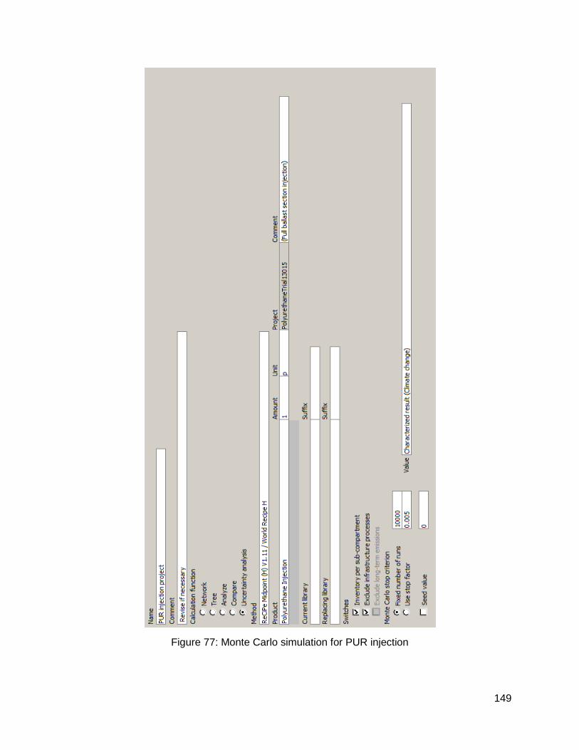
149
Figure 77: Monte Carlo simulation for PUR injection

150
Figure 78: LCCA calculation for ballast at 10% discount rate

151
Appendix C: Proposed instrumentation
Rail reflectors Berntsen RSAK130 adapter with smart-angle-retro-reflective survey targets will be installed on
the web on the rail with epoxy construction adhesive (Figure 79). Placement will be every 2-m.
Upon finalization of the injection lengths, reflectors should be installed the day prior to PUR
injections and an initial reading should be conducted. With any/all the left over targets, the control
section (South Approach) should be installed in a similar method. If there are no reflective-
markers left, PK-nails with tags should be installed on the fastener of the rail to tie to mark survey
points. Then a prism with rod will be used to take measurements. Traditional total-station surveys
will be conducted with these reflectors and a prism. A relative benchmark will need to be
established during the first survey, a concrete bridge abutment would be a good choice.
Figure 79: RSAK130 target
Settlement gauges
A modified Borros-type settlement gauge will be constructed and installed at multiple locations
along the injected and control section (Figure 80). One should be placed close to the bridge
abutment and then wherever different injection procedures are used. A 25.4 mm inner-diameter
galvanized steel pipe will function as the sleeve in which the settlement rod is measured. A heavy-
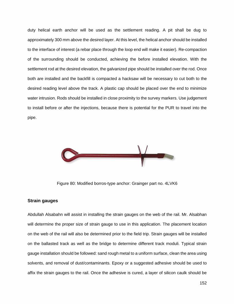
152
duty helical earth anchor will be used as the settlement reading. A pit shall be dug to
approximately 300 mm above the desired layer. At this level, the helical anchor should be installed
to the interface of interest (a rebar place through the loop end will make it easier). Re-compaction
of the surrounding should be conducted, achieving the before installed elevation. With the
settlement rod at the desired elevation, the galvanized pipe should be installed over the rod. Once
both are installed and the backfill is compacted a hacksaw will be necessary to cut both to the
desired reading level above the track. A plastic cap should be placed over the end to minimize
water intrusion. Rods should be installed in close proximity to the survey markers. Use judgement
to install before or after the injections, because there is potential for the PUR to travel into the
pipe.
Figure 80: Modified borros-type anchor: Grainger part no. 4LVK6
Strain gauges
Abdullah Alsabahn will assist in installing the strain gauges on the web of the rail. Mr. Alsabhan
will determine the proper size of strain gauge to use in this application. The placement location
on the web of the rail will also be determined prior to the field trip. Strain gauges will be installed
on the ballasted track as well as the bridge to determine different track moduli. Typical strain
gauge installation should be followed: sand rough metal to a uniform surface, clean the area using
solvents, and removal of dust/contaminants. Epoxy or a suggested adhesive should be used to
affix the strain gauges to the rail. Once the adhesive is cured, a layer of silicon caulk should be

153
placed over the strain gauges to weatherproof them. Readings should be taken as often as
possible with passing trains.