Copyright © 2011 Pearson Education, Inc. Analysis of Variance Chapter 26

Copyright © 2011 Pearson Education, Inc.

Analysis of Variance

Chapter 26

26.1 Comparing Several Groups

Did agricultural yield go up this year because of more fertilizer or more rain? Or is it the result of temperature or type of seed used?

Use regression analysis with dummy variables to compare the averages of several groups.

This approach is also known as analysis of variance.


3 of 42


Which Wheat Variety Should a Farmer Plant?

Five varieties of wheat are being considered: Endurance, Hatcher, NuHills, RonL, and Ripper.

Each variety was grown in randomly chosen plots and yield was measured as bushels per acre.

Balanced experiment: experiment with an equal number of observations for each treatment.


4 of 42


Steps to Follow in the Analysis

Plot the data to find patterns.

Propose a regression model for the data.

Check conditions associated with the model.

Test hypotheses and draw a conclusion.


5 of 42


Comparing Groups in Plots – Boxplots of Yield


6 of 42


Comparing Groups in Plots – Summary Statistics


7 of 42


Relating the t-Test to Regression

Is there a significant difference between the average yield of Endurance and the others?

Since the variances among groups appear similar, use the two sample t-test and pool the variances.


8 of 42



The t-statistic and p-value show that Endurance has a significantly higher mean yield per acre than the combination of other varieties.


9 of 42



The t-test can be formulated as a regression with a dummy variable D(Endurance) that is coded 1 if plot is seeded with Endurance and 0 otherwise.


10 of 42



The slope b1 = 5.53 matches the estimate for the difference between means.

Testing the slope is equivalent to a pooled two-sample t-test of the difference between means (the t-statistic and p-value are the same).


11 of 42


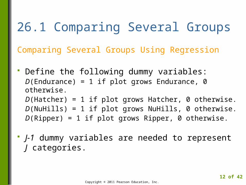
Comparing Several Groups Using Regression

Define the following dummy variables:D(Endurance) = 1 if plot grows Endurance, 0 otherwise.D(Hatcher) = 1 if plot grows Hatcher, 0 otherwise.D(NuHills) = 1 if plot grows NuHills, 0 otherwise.D(Ripper) = 1 if plot grows Ripper, 0 otherwise.

J-1 dummy variables are needed to represent J categories.


12 of 42



The variety RonL is the baseline category (defined by all zeros for the dummy variables).

Analysis of variance (ANOVA): the comparison of two or more averages using regression model with all dummy variables.


13 of 42




14 of 42


Interpreting the Estimates

The slope of each dummy variable compares the average response of its category to the average of the baseline category.

If D(Endurance) = 1, we find = 19.58 bushels per acre. Since b0 = 11.68 is the mean yield for RonL, the slope for D(Endurance), which is b1 = 7.9 is the difference between the average yields.


15 of 42

y


ANOVA Regression Model

The equation of the MRM for the Wheat example can be written in terms of the population means:


16 of 42

)()()()( 52515 HatcherDEnduranceDy

)()()()( 5453 RipperDNuHillsD


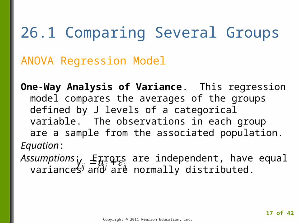
ANOVA Regression Model

One-Way Analysis of Variance. This regression model compares the averages of the groups defined by J levels of a categorical variable. The observations in each group are a sample from the associated population.

Equation:Assumptions: Errors are independent, have equal

variances and are normally distributed.


17 of 42

ijjijy

26.2 Inference in ANOVA Regression Models

Checking Conditions

Linear association: automatic for ANOVA. No obvious lurking variable: automatic if data are

from a randomized experiment (i.e., wheat example).

Check the remaining conditions (independence, similar variances, and normality) with appropriate residual plots.


18 of 42


Checking Conditions

If IQR’s are similar, within a factor of 3 to 1 with up to five groups, similar variances condition is met.


19 of 42


Checking Conditions

Residuals appear nearly normal.


20 of 42


F-Test for the Difference among Means

Used to test the following null hypothesis:H0: µ1 = µ2 = µ3 = µ4 = µ5

Typically summarized in an ANOVA table:

The p-value < 0.05; reject H0.


21 of 42


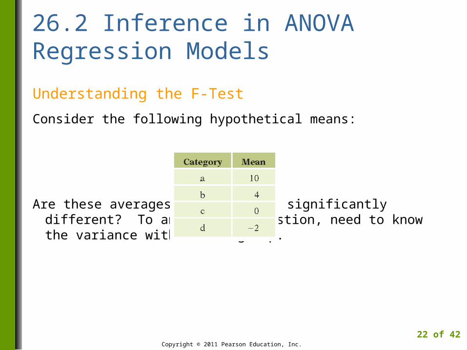
Understanding the F-Test

Consider the following hypothetical means:

Are these averages statistically significantly different? To answer this question, need to know the variance within each group.


22 of 42


Understanding the F-Test

Both plots show groups with the same averages, but different within group variances. No significant differences in averages in right plot.


23 of 42


Confidence Intervals

Since the F-test shows that the mean yields among varieties of wheat are not the same, which variety is best?


24 of 42

26.3 Multiple Comparisons

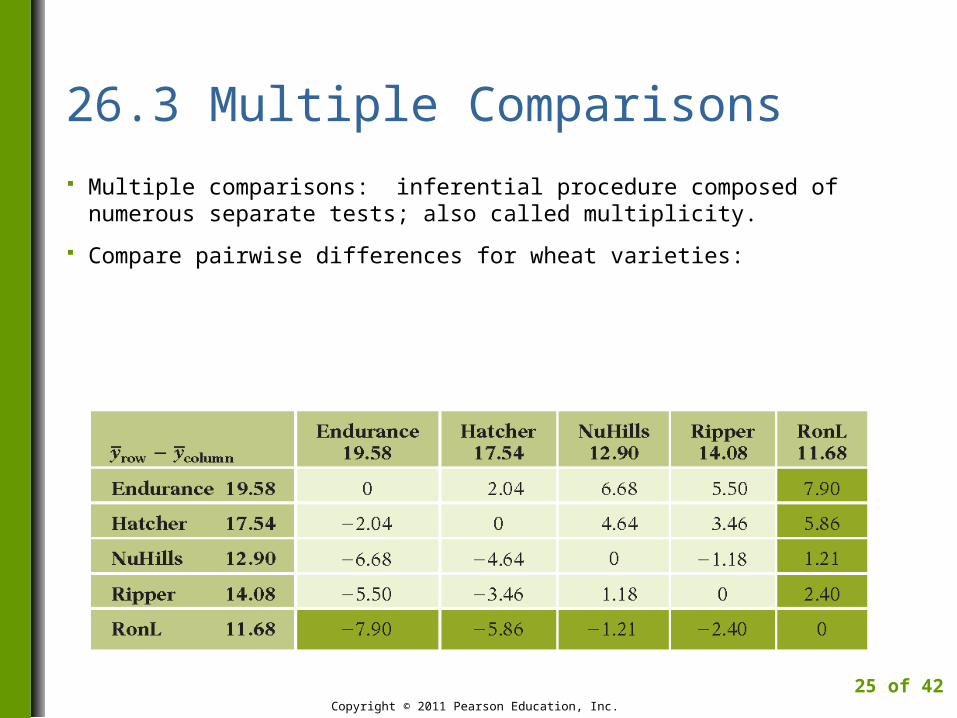
Multiple comparisons: inferential procedure composed of numerous separate tests; also called multiplicity.

Compare pairwise differences for wheat varieties:


25 of 42


Tukey Confidence Intervals

These intervals hold the chance for a Type I error to 5% over the entire collection of pairwise comparisons.

Replaces the t-percentile in confidence intervals with a larger multiple of the standard error (obtained from a special table).


26 of 42


Tukey Confidence Intervals - Wheat Example

The 95% Tukey confidence interval for the two best varieties of wheat (Endurance and Hatcher):

2.04 ± 2.875 2.11 = 2.04 ± 6.07 bushels/acre

This difference is not statistically significant since the Tukey interval includes 0.


27 of 42


Tukey Confidence Intervals - Wheat Example

Note that the width of the 95% Tukey confidence interval is the same for any pairwise comparison.

The difference in yield between any two varieties compared must be more than 6.07 bushels/acre in order to be statistically significant.


28 of 42


Bonferroni Confidence Intervals

These intervals adjust for multiple comparisons by changing the α level used in the standard interval to α/M for M intervals.

For the comparison among wheat varieties, Bonferroni confidence intervals reduce α = 0.05 to α/10 = 0.005 and replaced t = 2.08 with t = 3.00.


29 of 42

26.4 Groups of Different Size

With groups of different sizes, unbalanced data produce confidence intervals of different widths.

Compute the estimated standard error for a pairwise comparison using the following formula with relevant sample sizes:


30 of 42

2121

11)(

nnsyyse e

4M Example 26.1: JUDGING THE CREDIBILITY OF ADVERTISEMENTS

Motivation

Advertising executives want to compare four commercials for a retail item that make claims of varying strengths. Specifically, they want to know how over-the-top an ad can be before customers turn away in disbelief.


31 of 42


Method

The data consist of reactions for a sample of 80 customers who viewed commercials with claims in one of four categories: Tame, Plausible, Stretch and Outrageous. Each customer was randomly assigned to a commercial. The response variable is Credibility obtained by customers’ responses to items on a questionnaire they completed after viewing the ad.


32 of 42


Method

Use regression with three dummy variables to capture the four types of claims made in the commercials. Check the conditions for ANOVA. Linearity is not an issue and there are no obvious lurking variables because randomization was used in designing the study.


33 of 42


Mechanics - Results


34 of 42


Mechanics – Results


35 of 42


Mechanics – Check remaining conditions before proceeding with

inference.

Similar variances condition is satisfied.


36 of 42


Mechanics –Check remaining conditions before proceeding with

inference.

Nearly normal condition is satisfied.


37 of 42


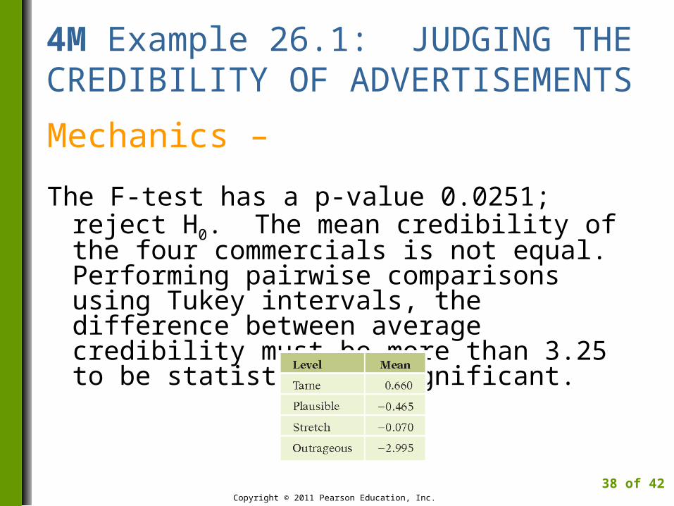
Mechanics –

The F-test has a p-value 0.0251; reject H0. The mean credibility of the four commercials is not equal. Performing pairwise comparisons using Tukey intervals, the difference between average credibility must be more than 3.25 to be statistically significant.


38 of 42


Message

Based on the Tukey intervals, there is only one statistically significant pairwise difference (between commercials making tame claims and those that make outrageous). Customers place less credibility in ads that make outrageous claims than ads that make tame claims.


39 of 42

Best Practices

Use a randomized experiment to obtain data.

Check the assumptions of multiple regression when using ANOVA regression.

Use Tukey or Bonferroni confidence intervals to identify groups that are significantly different.

Recognize the cost of snooping in the data to choose hypotheses.


40 of 42

Pitfalls

Don’t compare the means of several groups using lots of t-tests.

Don’t forget confounding factors.

Never pretend you have only two groups.


41 of 42

Pitfalls (Continued)

Do not add or subtract standard errors.

Do not use a one-way ANOVA to analyze data with repeated measurements


42 of 42

Documents

Copyright © 2011 Pearson Education, Inc. Analysis of Variance Chapter 26