Copyright © 2009 Pearson Education, Inc. Chapter 6 The Standard Deviation As A Ruler And The Normal Model

Copyright © 2009 Pearson Education, Inc.

Chapter 6The Standard Deviation

As A Ruler And

The Normal Model

Copyright © 2009 Pearson Education, Inc. Slide 1- 2

The Standard Deviation as a Ruler

The trick in comparing very different-looking values is to use standard deviations as our rulers.

The standard deviation tells us how the whole collection of values varies, so it’s a natural ruler for comparing an individual to a group.

As the most common measure of variation, the standard deviation plays a crucial role in how we look at data.


ILLUSTRATIVE EXAMPLE

AN OLYMPIC COMMITTEE LOOKS AT THE PERFORMANCES OF TWO OLYMPIC ATHLETES

BACHER WINNING 800 METERS IN 129 SECONDS

PROKHOROVA WINNING LONG JUMP WITH 660 CENTIMETERS JUMP

BOTH ATHLETES WON GOLD IN THEIR RESPECTIVE DISCIPLINE. WHO WAS THE BETTER ATHLETE?

Slide 1- 3


TO ANSWER, WE NEED TO STANDARDIZE THE RESULTS. HOW?

FIRST: GET A BASE VALUE FOR COMPARISON. THE MEAN SHALL BE OUR BASE VALUE.

SECOND: WE NEED TO KNOW HOW FAR AWAY (DEVIATION) WE ARE FROM THE MEAN.

THE STANDARD DEVIATION WILL SERVE AS THAT RULER OF MEASUREMENT.

Slide 1- 4


Standardizing with z-scores

We compare individual data values to their mean, relative to their standard deviation using the following formula:

We call the resulting values standardized values, denoted as z. They can also be called z-scores.

z

y y s


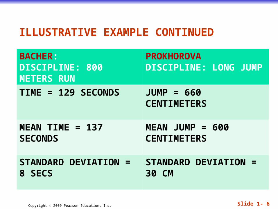
ILLUSTRATIVE EXAMPLE CONTINUED

BACHER:DISCIPLINE: 800 METERS RUN

PROKHOROVADISCIPLINE: LONG JUMP

TIME = 129 SECONDS JUMP = 660 CENTIMETERS

MEAN TIME = 137 SECONDS

MEAN JUMP = 600 CENTIMETERS

STANDARD DEVIATION = 8 SECS

STANDARD DEVIATION = 30 CM

Slide 1- 6


NOW LET US STANDARDIZE THE PERFORMANCES OF THESE ATHLETES

Slide 1- 7


STANDARDIZING PERFORMANCES CONTINUED

Slide 1- 8


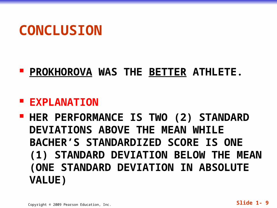
CONCLUSION

PROKHOROVA WAS THE BETTER ATHLETE.

EXPLANATION HER PERFORMANCE IS TWO (2) STANDARD

DEVIATIONS ABOVE THE MEAN WHILE BACHER’S STANDARDIZED SCORE IS ONE (1) STANDARD DEVIATION BELOW THE MEAN (ONE STANDARD DEVIATION IN ABSOLUTE VALUE)

Slide 1- 9


EXAMPLE

A TOWN’S JANUARY HIGH TEMPERATURES AVERAGE 36 DEGREES WITH A STANDARD DEVIATION OF 10 DEGREES, WHILE IN JULY THE MEAN HIGH TEMPERATURE IS 74 DEGREES AND THE STANDARD DEVIATION IS 8 DEGREES. IN WHICH MONTH IS IT MORE UNSUAL TO HAVE A DAY WITH A HIGH TEMPERATURE OF 55 DEGREES? EXPLAIN.

Slide 1- 10


EXAMPLE

AN INCOMING FRESHMAN TOOK HER COLLEGE’S PLACEMENT EXAMS IN FRENCH AND MATHEMATICS. IN FRENCH, SHE SCORED 82 AND IN MATH 86. THE OVERALL RESULTS ON THE FRENCH EXAM HAD A MEAN OF 72 AND A STANDARD DEVIATION OF 8, WHILE THE MEAN MATH SCORE WAS 68, WITH A STANDARD DEVIATION OF 12. ON WHICH EXAM DID SHE DO BETTER COMPARED WITH THE OTHER FRESHMEN?

Slide 1- 11


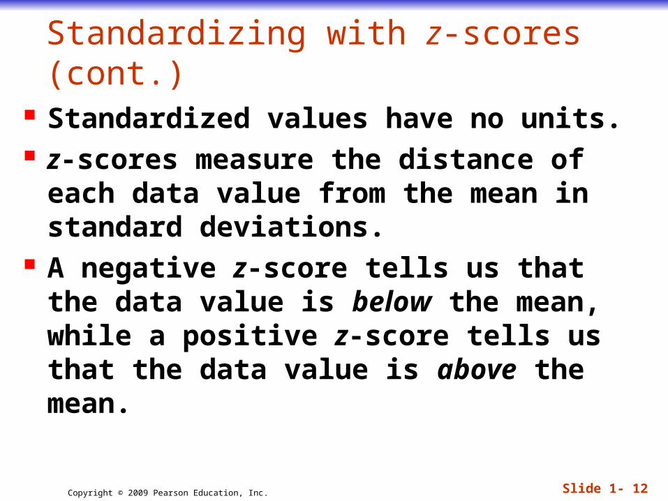
Standardizing with z-scores (cont.) Standardized values have no units. z-scores measure the distance of each

data value from the mean in standard deviations.

A negative z-score tells us that the data value is below the mean, while a positive z-score tells us that the data value is above the mean.


Benefits of Standardizing

Standardized values have been converted from their original units to the standard statistical unit of standard deviations from the mean.

Thus, we can compare values that are measured on different scales, with different units, or from different populations.


Shifting Data

Shifting data: Adding (or subtracting) a constant to every

data value adds (or subtracts) the same constant to measures of position.

Adding (or subtracting) a constant to each value will increase (or decrease) measures of position: center, percentiles, max or min by the same constant.

Its shape and spread - range, IQR, standard deviation - remain unchanged.


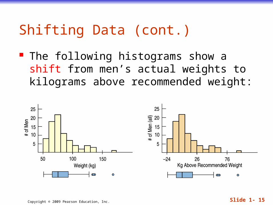
Shifting Data (cont.)

The following histograms show a shift from men’s actual weights to kilograms above recommended weight:


Rescaling Data

Rescaling data: When we multiply (or divide) all the data

values by any constant, all measures of position (such as the mean, median, and percentiles) and measures of spread (such as the range, the IQR, and the standard deviation) are multiplied (or divided) by that same constant.


Rescaling Data (cont.)

The men’s weight data set measured weights in kilograms. If we want to think about these weights in pounds, we would rescale the data:


CLASS EXAMPLES

TEXTBOOK PAGE 148

Slide 1- 18


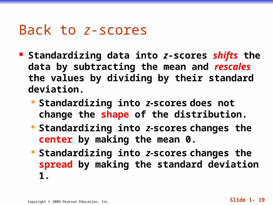
Back to z-scores

Standardizing data into z-scores shifts the data by subtracting the mean and rescales the values by dividing by their standard deviation. Standardizing into z-scores does not

change the shape of the distribution. Standardizing into z-scores changes the

center by making the mean 0. Standardizing into z-scores changes the

spread by making the standard deviation 1.


When Is a z-score BIG?

A z-score gives us an indication of how unusual a value is because it tells us how far it is from the mean.

Remember that a negative z-score tells us that the data value is below the mean, while a positive z-score tells us that the data value is above the mean.

The larger a z-score is (negative or positive), the more unusual it is.


When Is a z-score Big? (cont.)

There is no universal standard for z-scores, but there is a model that shows up over and over in Statistics.

This model is called the Normal model (You may have heard of “bell-shaped curves.”).

Normal models are appropriate for distributions whose shapes are unimodal and roughly symmetric.

These distributions provide a measure of how extreme a z-score is.



There is a Normal model for every possible combination of mean and standard deviation. We write N(μ,σ) to represent a Normal

model with a mean of μ and a standard deviation of σ.

We use Greek letters because this mean and standard deviation do not come from data—they are numbers (called parameters) that specify the model.



Summaries of data, like the sample mean and standard deviation, are written with Latin letters. Such summaries of data are called statistics.

When we standardize Normal data, we still call the standardized value a z-score, and we write

yz



Once we have standardized, we need only one model: The N(0,1) model is called the standard

Normal model (or the standard Normal distribution).

Be careful—don’t use a Normal model for just any data set, since standardizing does not change the shape of the distribution.



When we use the Normal model, we are assuming the distribution is Normal.

We cannot check this assumption in practice, so we check the following condition: Nearly Normal Condition: The shape of the

data’s distribution is unimodal and symmetric.

This condition can be checked by making a histogram or a Normal probability plot (to be explained later).


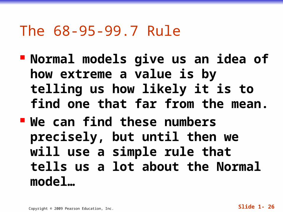
The 68-95-99.7 Rule

Normal models give us an idea of how extreme a value is by telling us how likely it is to find one that far from the mean.

We can find these numbers precisely, but until then we will use a simple rule that tells us a lot about the Normal model…


The 68-95-99.7 Rule (cont.)

It turns out that in a Normal model: about 68% of the values fall within one

standard deviation of the mean; about 95% of the values fall within two

standard deviations of the mean; and, about 99.7% (almost all!) of the values

fall within three standard deviations of the mean.


The 68-95-99.7 Rule (cont.)

The following shows what the 68-95-99.7 Rule tells us:


CLASS EXAMPLES

TEXTBOOK PAGE 149

Slide 1- 29


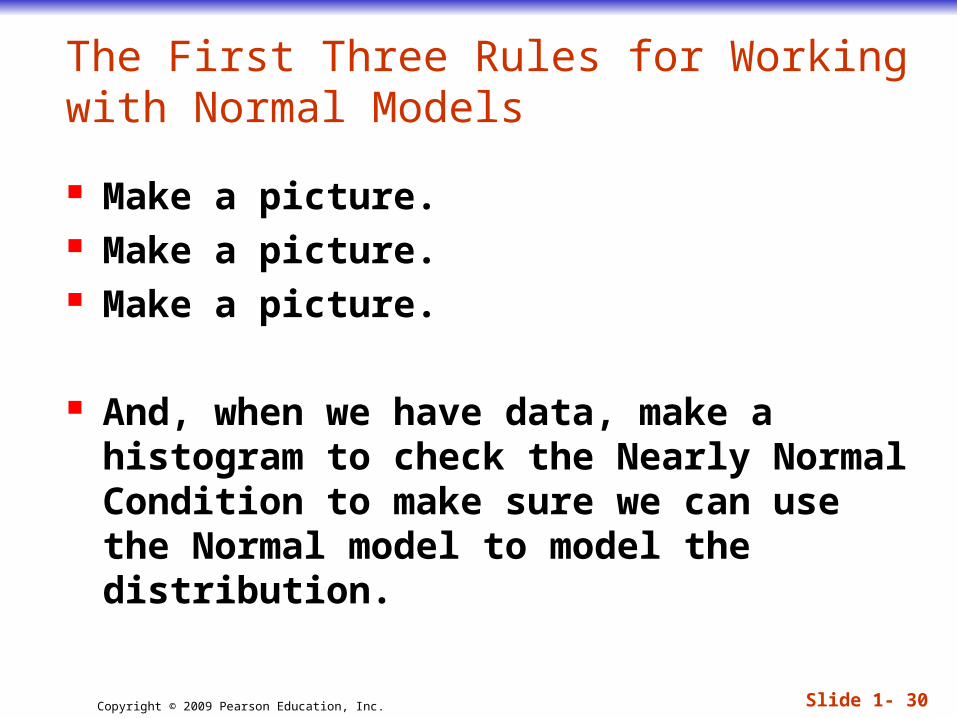
The First Three Rules for Working with Normal Models

Make a picture. Make a picture. Make a picture.

And, when we have data, make a histogram to check the Nearly Normal Condition to make sure we can use the Normal model to model the distribution.


Finding Normal Percentiles by Hand

When a data value doesn’t fall exactly 1, 2, or 3 standard deviations from the mean, we can look it up in a table of Normal percentiles.

Table Z in Appendix D provides us with normal percentiles, but many calculators and statistics computer packages provide these as well.


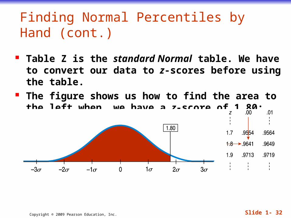
Finding Normal Percentiles by Hand (cont.)

Table Z is the standard Normal table. We have to convert our data to z-scores before using the table.

The figure shows us how to find the area to the left when we have a z-score of 1.80:


Finding Normal Percentiles Using Technology

Many calculators and statistics programs have the ability to find normal percentiles for us.

The ActivStats Multimedia Assistant offers two methods for finding normal percentiles:

The “Normal Model Tool” makes it easy to see how areas under parts of the Normal model correspond to particular cut points.

There is also a Normal table in which the picture of the normal model is interactive.


Finding Normal Percentiles Using Technology (cont.)

The following was produced with the “Normal Model Tool” in ActivStats:


From Percentiles to Scores: z in Reverse

Sometimes we start with areas and need to find the corresponding z-score or even the original data value.

Example: What z-score represents the first quartile in a Normal model?


From Percentiles to Scores: z in Reverse (cont.)

Look in Table Z for an area of 0.2500. The exact area is not there, but 0.2514 is

pretty close.

This figure is associated with z = -0.67, so the first quartile is 0.67 standard deviations below the mean.


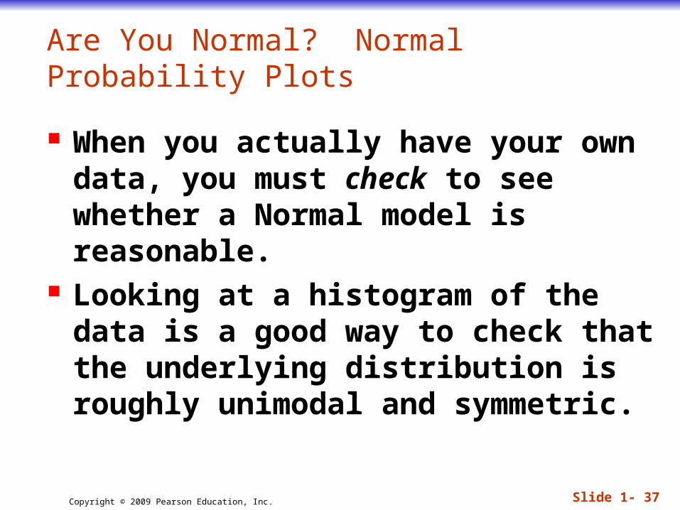
Are You Normal? Normal Probability Plots

When you actually have your own data, you must check to see whether a Normal model is reasonable.

Looking at a histogram of the data is a good way to check that the underlying distribution is roughly unimodal and symmetric.


A more specialized graphical display that can help you decide whether a Normal model is appropriate is the Normal probability plot.

If the distribution of the data is roughly Normal, the Normal probability plot approximates a diagonal straight line. Deviations from a straight line indicate that the distribution is not Normal.

Are You Normal? Normal Probability Plots (cont)


Nearly Normal data have a histogram and a Normal probability plot that look somewhat like this example:



A skewed distribution might have a histogram and Normal probability plot like this:



What Can Go Wrong?

Don’t use a Normal model when the distribution is not unimodal and symmetric.


What Can Go Wrong? (cont.)

Don’t use the mean and standard deviation when outliers are present—the mean and standard deviation can both be distorted by outliers.

Don’t round your results in the middle of a calculation.

Don’t worry about minor differences in results.


What have we learned?

The story data can tell may be easier to understand after shifting or rescaling the data. Shifting data by adding or subtracting the

same amount from each value affects measures of center and position but not measures of spread.

Rescaling data by multiplying or dividing every value by a constant changes all the summary statistics—center, position, and spread.


What have we learned? (cont.)

We’ve learned the power of standardizing data. Standardizing uses the SD as a ruler to

measure distance from the mean (z-scores). With z-scores, we can compare values from

different distributions or values based on different units.

z-scores can identify unusual or surprising values among data.


We’ve learned that the 68-95-99.7 Rule can be a useful rule of thumb for understanding distributions: For data that are unimodal and symmetric,

about 68% fall within 1 SD of the mean, 95% fall within 2 SDs of the mean, and 99.7% fall within 3 SDs of the mean.




We see the importance of Thinking about whether a method will work: Normality Assumption: We sometimes work

with Normal tables (Table Z). These tables are based on the Normal model.

Data can’t be exactly Normal, so we check the Nearly Normal Condition by making a histogram (is it unimodal, symmetric and free of outliers?) or a normal probability plot (is it straight enough?).


CLASS EXAMPLES

TEXTBOOK PAGES 151 - 152

Slide 1- 47

Documents

Copyright © 2009 Pearson Education, Inc. Chapter 6 The Standard Deviation As A Ruler And The Normal Model