Copyright © 2006 M-OSRP Inc. All rights reserved. Report 2001-2002.pdf · Petrobras Jurandyr Schmidt Phillips Doug Foster Saudi Aramco Panos Kelamis Shell Jon Sheiman (Chairman)

HomeAbout M-OSRPPeopleResearchEventsSponsorsLinks

Contact M-OSRP

1. Introduction to MOSRP01A. B. Weglein

2. Philosophy and strategy or M-OSRP

3. Sponsors

4. Students, faculty and collaboration

5. Objectives and tools (Math-Physics)

6. Preprocessing: wavefield prediction, wavelet estimation, anddeghosting

7. Forward and inverse series and imaging subseries

8. Inversion - near-source trace extrapolation

Table of Contents

www.mosrp.uh.edu http://www.mosrp.uh.edu/secure/meeting0102.html

1 of 2 7/25/2013 1:04 PM

Copyright © 2006 M-OSRP Inc. All rights reserved.

www.mosrp.uh.edu http://www.mosrp.uh.edu/secure/meeting0102.html

2 of 2 7/25/2013 1:04 PM

Summary As a means of introduction, this report begins with the presentation slides that were used to propose the M-OSRP program to the university community and to the petroleum industry. They describe the philosophy, objectives and strategy that define, motivate and guide this program – that is, to serve the aligned interests of prioritized fundamental seismic science, the petroleum industry, and the core educational responsibility of the university. The industry response to our invitation to participate and sponsor our new program was overwhelmingly positive. A list of our petroleum industry sponsors, and their Advisory Board members, and associate sponsors is included. This is followed by a list of our students and faculty. The high level of support, participation and collaboration is both encouraging and gratifying. Our technical strategy and plan are then described followed by a list of our Ph.D. students and their research projects. The section that follows describes the math-physics tools that form the foundation for the methods we develop, test and apply. These methods are specifically designed to improve our ability to unravel seismic data. They allow us to separate the information about the portion of the wavefield’s history that we are interested in from the myriad of factors that have influenced its character. The flexibility of the method used to describe how data experienced the Earth determines how flexible and cooperative the data will be to reveal its history when using that method in an inverse sense as a processing tool. The methods we seek are multidimensional and heterogeneous and allow the maximum number of channels and realism for the data while requiring only realistic achievable levels of a priori information. The inverse scattering series is the maximally flexible deterministic tool available today for relating reflection data to subsurface properties. As these methods reduce the unrealistic assumptions about the subsurface, they place a greater burden, demand and responsibility on the definition and completeness of the seismic experiment. The wavefield prediction, extrapolation, wavelet estimation, and deghosting projects are our response to that challenge and derive from direct inversion, indirect inversion or various forms of the Extinction Theorem. In addition, statistical methods are sought to accommodate the uncertainties inherent between reality and deterministic methods. When combined with new acquisition (e.g., point wavefield measurements), this trend from unrealistic assumptions about the subsurface to greater expectations about the definition and completeness of the seismic experiment, represents an empowerment where those interested in spending more have the opportunity of achieving more. M-OSRP and this report are aligned with this objective. In this document, the objectives and status of individual projects are described by reports, notes, expanded abstracts and manuscripts. The five current projects are: wavefield and wavelet estimation, data reconstruction and near source interpolation in shallow water, imaging at depth without the precise velocity, inversion of complex large contrast targets, and velocity analysis. There are fundamental studies and reports that support and guide

these projects. Since we are committed to working on relevant high prioritized outstanding technical challenges, we anticipate that significant attention at the embryonic stages of projects would be paid to problem definition, solution concept development, and analytic and numerical data tests. The projects in M-OSRP represent a portfolio of different risk and timetables for deliverables. The expectation is that the Extinction Theorem derived wavefield prediction, wavelet estimation and deghosting algorithms will be the first to be tested for added value on field data followed by data reconstruction, and near source extrapolation. The demonstrated cooperation between successive terms in the imaging at depth (without the velocity) subseries and the numerical testing results for 1-D normal incidence models are encouraging. Further analysis and testing are planned. The program will maintain the current balance between seeking new enabling capability for locating and identifying targets and new processing techniques (when combined with advances in acquisition) that meet the heightened demands (prerequisites) on completeness and definition of the seismic experiment. Arthur B. Weglein Director, M-OSRP University of Houston December 6th, 2001

Tier I Sponsors

Company Advisory Board Member

Amerada Hess Jacques Leveille BP Nigel Purnell

Chevron Ray Ergas / Debbie Bones Conoco Robert H. Stolt

ENI-Agip Michele Buia Exxon-Mobil Nizar Chemingui

GX Technology Nick Bernitsas Petrobras Jurandyr Schmidt Phillips Doug Foster

Saudi Aramco Panos Kelamis Shell Jon Sheiman (Chairman)

Statoil Lasse Amundsen Texaco John Riola / Joseph Higginbotham

Total Fina Elf Claude Lafond Unocal Phil Schultz

WesternGeco Luis Canales

Tier II Sponsors (Working Team contributions or participating student support)

Company Contact

ADS Bee Bednar CGG Simon Spitz

Stochastic Systems Suresh Thadani

Active collaborating universities

University Contact

U.T. Austin, U.T.I.G.* Paul Stoffa, Mrinal Sen U. British Columbia,

C.D.S.S.T Tadeusz Ulrych, Michael

Bostock U.C. Santa Cruz Ru-Shan Wu Delft University A.J. Berkhout, Dries Gisolf,

Jacob Fokkema *We thank BP for supporting this collaborative research. The Margaret S. and Robert E. Sheriff Endowment is recognized for support and encouragement of this research program.

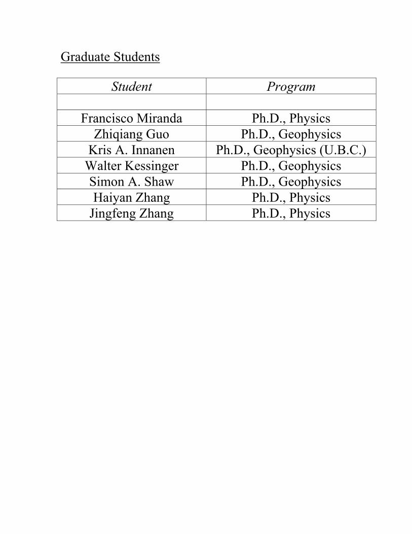
Graduate Students

Student Program

Francisco Miranda Ph.D., Physics Zhiqiang Guo Ph.D., Geophysics

Kris A. Innanen Ph.D., Geophysics (U.B.C.) Walter Kessinger Ph.D., Geophysics Simon A. Shaw Ph.D., Geophysics Haiyan Zhang Ph.D., Physics

Jingfeng Zhang Ph.D., Physics

Faculty

Faculty Affiliation

Gustavo Correa (p.t.) Geosciences Bogdan Nita Physics

Arthur B. Weglein Geosciences and Physics

Associated Faculty

Faculty Affiliation

Don Kouri Physics Carlos Ordonez Physics

Mission-Oriented Seismic Research Program

September 7, 2001 1


Update, Issues and Plan Forward

September 7, 2001University of Houston


September 7, 2001 2

Objectives• Develop and evaluate methods to: (1) image beneath complex media, and (2) identify large contrast structurally complex (e.g., curved, corrugated diffractive) targets

• Develop and evaluate methods for satisfying the intrinsic and practical prerequisites of these techniques


September 7, 2001 3

Overall StrategyLocate Identify (invert)

Invert at ocean bottom

Accurately locate target (space) beneath complex

medium

Invert where time migration is adequate (e.g., 4-D)

Locate beneath complex medium and then invert a complex target


September 7, 2001 4

Projects• Velocity Analysis• Imaging at depth without the velocity model• Inverting large-contrast and complex targets• Prerequisite satisfaction• Data mapping• Near-source traces in shallow water•Wavefield above cable and wavelet from the Extinction Theorem (E.T.)• Deghosting (E.T.)• Comparing subtraction techniques for 2-D – 3-D models: pattern recognition, energy minimization and wavelet estimation (E.T.)


September 7, 2001 5

Graduate Students (all Ph.D. candidates)

Francisco M. Fernandez PhysicsZhiqiang Guo GeophysicsKristopher Innanen Geophysics (UBC)

Walter Kessinger GeophysicsSimon Shaw GeophysicsHaiyan Zhang PhysicsJingfeng Zhang Physics


September 7, 2001 6

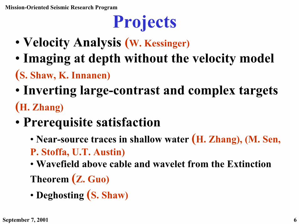
Projects• Velocity Analysis (W. Kessinger)• Imaging at depth without the velocity model (S. Shaw, K. Innanen)• Inverting large-contrast and complex targets (H. Zhang)• Prerequisite satisfaction• Near-source traces in shallow water (H. Zhang), (M. Sen, P. Stoffa, U.T. Austin)•Wavefield above cable and wavelet from the Extinction Theorem (Z. Guo)• Deghosting (S. Shaw)


September 7, 2001 7

Visiting Assistant Professors

Dr. Gustavo Correa (p.t.) GeophysicsDr. Bogdan Nita Physics

Associated FacultyProf. D. Kouri PhysicsProf. C. Ordonez Physics


September 7, 2001 8

The Four Tasks of Direct Inversion

(1) Free surface demultiple

(2) Internal demultiple

(3) Image reflectors at depth

(4) Determine medium properties


September 7, 2001 9

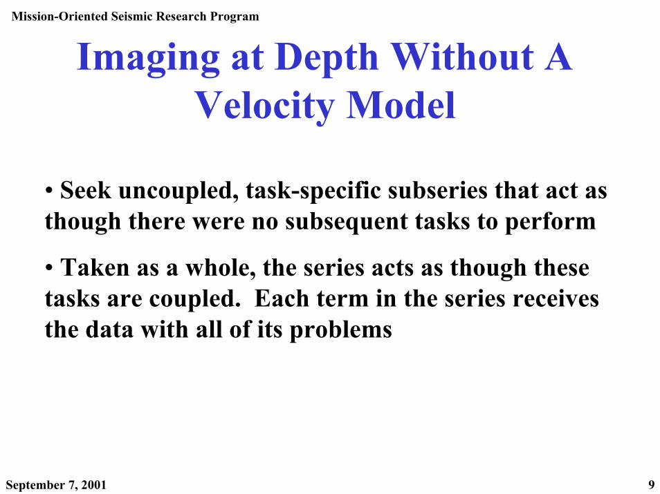
Imaging at Depth Without A Velocity Model

• Seek uncoupled, task-specific subseries that act as though there were no subsequent tasks to perform

• Taken as a whole, the series acts as though these tasks are coupled. Each term in the series receives the data with all of its problems


September 7, 2001 10


•We have determined the diagram (algorithm) corresponding to task (3) in the series

•We are looking at the issue of isolating task (3) from task (4). We know where task (4) is on its own

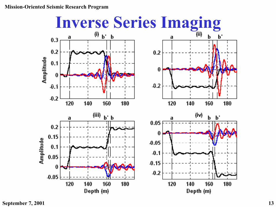
• Initial 1-D testing of algorithm corresponding to the simplest realization of the diagram and bandlimiteddata is encouraging (S. Shaw)

• Plan to extend testing to more complicated pre-stack 1-D models. Determine quantity to take through diagram that is best suited for imaging



Inverse Series Imaging









Imaging Without Velocity – Plan1. Complete fundamental analysis of task

isolation and related issues

2. V(z) reference:• Analytic WKBJ migration

• Test with synthetic 1-D and 2-D media, field data test

3. V(x,z) reference:• Use phase-screen migration (Ru-Shan Wu)

• Exchange migration and imaging series results without exchange of code

• Test and evaluate




Development of basic concepts, algorithm development and testing: S. Shaw

Forward series with absorption. Impact of absorption on inverse series. In particular, how would including an estimate of Q with reference medium (Green’s function) affect imaging at depth? K. Innanen



Prerequisite Satisfaction•Wavefield prediction and wavelet estimation (Z. Guo)• 2-D codes complete and initial synthetic testing under way• Deghosting from extinction theorem (S. Shaw)• Tests will include impact on demultiple and imaging

(Prof. Correa has generated a series of model data sets for evaluation of wavefield prediction, wavelet estimation, anddeghosting)



Synthetic seismograms for M-OSRP

Gustavo Correa



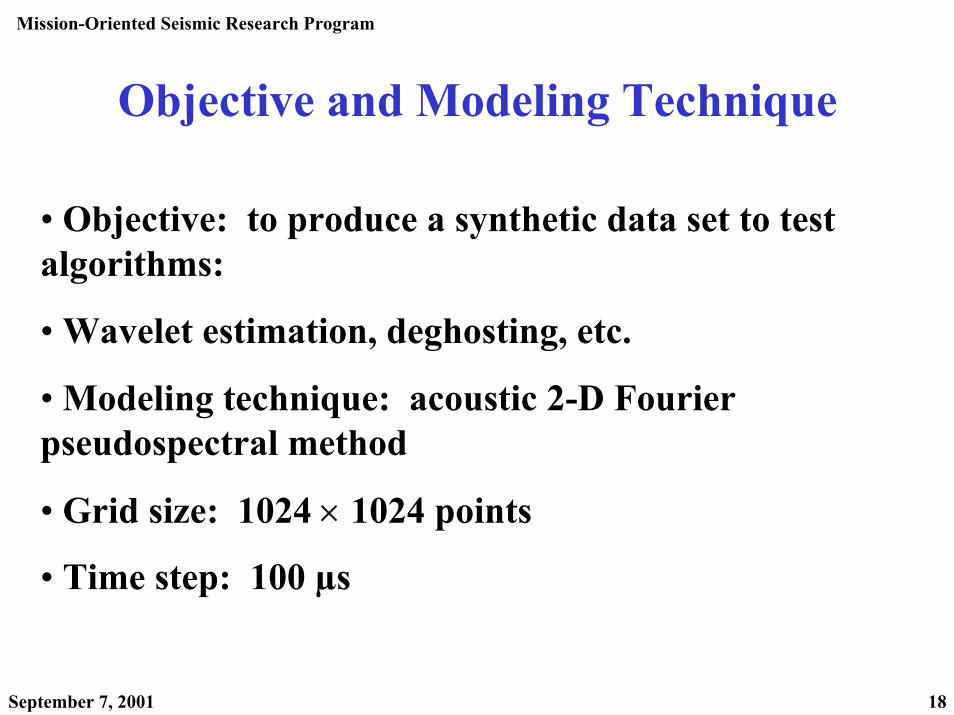
Objective and Modeling Technique

• Objective: to produce a synthetic data set to test algorithms:

•Wavelet estimation, deghosting, etc.

•Modeling technique: acoustic 2-D Fourierpseudospectral method

• Grid size: 1024 × 1024 points

• Time step: 100 µs



Model Parameters• One to three layers:

• Basement traveltime = 1st. sea floor multipletraveltime at zero offset.

-26404500Basement

75024002250Sediments

3001,0001,500Water

Depth (m)ρ (kg/m3)VP (m/s)Material



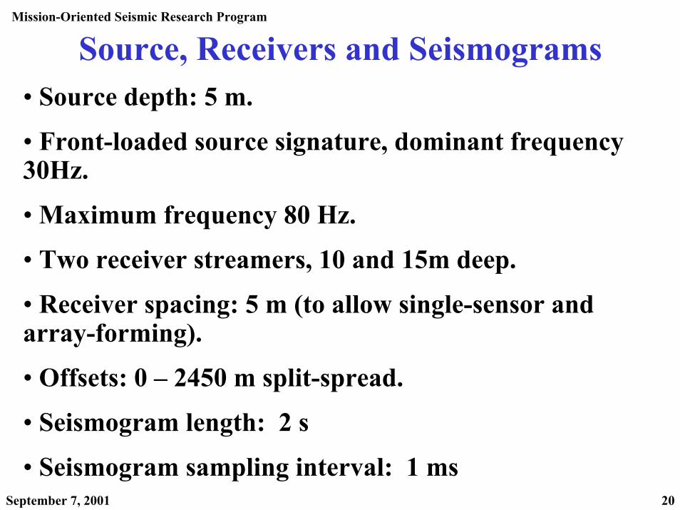
Source, Receivers and Seismograms• Source depth: 5 m.

• Front-loaded source signature, dominant frequency 30Hz.

•Maximum frequency 80 Hz.

• Two receiver streamers, 10 and 15m deep.

• Receiver spacing: 5 m (to allow single-sensor and array-forming).

• Offsets: 0 – 2450 m split-spread.

• Seismogram length: 2 s

• Seismogram sampling interval: 1 ms



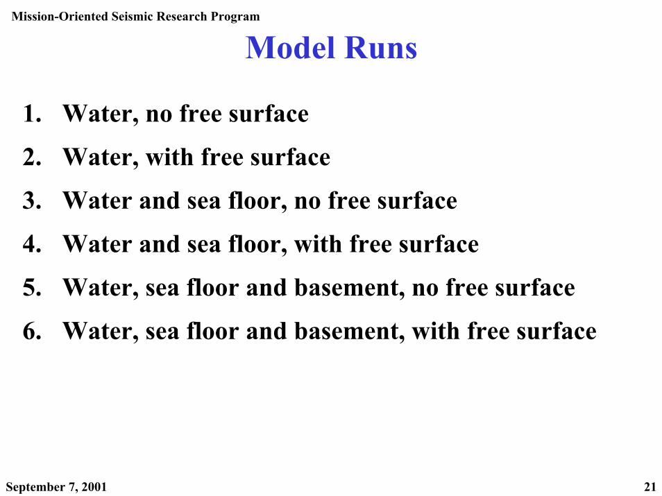
Model Runs

1. Water, no free surface

2. Water, with free surface

3. Water and sea floor, no free surface

4. Water and sea floor, with free surface

5. Water, sea floor and basement, no free surface

6. Water, sea floor and basement, with free surface







Primary and multiples interfere



Prerequisite Satisfaction (cont’d)

• A comparison of pattern recognition, energy minimization, and wavelet estimation for a set of 2D and 3D models – for multiple attenuation

•Working team will meet in October

• Data mapping – working team•Met at ADS in July 2001, will meet again in October



• Velocity Analysis (W. Kessinger)• Exchange of talks with W. Symes (Rice – TRIP)• All current constant offset, shot, or angle at target partial migrations show serious artifacts, even with perfect velocity•We have new (very recently developed) candidate method for MVA with potential to overcome these current obstacles to effectiveness. Will test and evaluate

• Inversion for large contrast, complex target identification: Task (4) (H. Zhang)

• Shallow water near trace interpolation; with M.Sen, P. Stoffa (UT Austin)

• For 2-D (3-D) water bottom, H. Zhang thesis

Prerequisite Satisfaction (cont’d)



Velocity Model Independent Imaging for Complex Media

(SEG Workshop, San Antonio, Sept. 14th)

• Invited overview talk – how do all of these imaging without the velocity methods relate to each other and to the imaging series and M-OSRP plans?



SEG Workshop Overview (cont’d)Wave-theoretic migration or asymptotic approximation

(Kirchhoff) migration, Green’s Theorem

Inverse Scattering Series

Interval velocity model not needed to find the reflectivity map at depth

Interval velocity model needed to find the reflectivity map at depth

No interval velocity ⇒ no depthimage of reflectivity

StackingNMO STK, DMO STK

CFP, CRS, CRE, time migrtn.For rapid rate of convergence a proximal velocity is usefulAll stacking methods seek

compromise: can we find imagewithout depth or reflectivity with a kinematic set of parameters to sum a moveout pattern



SEG Workshop Overview (cont’d)

• CFP, CRS, CRE, … represent approaches to imaging when estimated medium wave velocity is far from adequate



SEG Workshop Overview (cont’d)• NMO-STK and time migration concepts:

• NMO-STK requires a stacking velocity ~RMS velocity

• Put this in the Dix equation, and unphysical interval velocity can be predicted

• Is this a problem? No – it just shows that you can find an NMO-STK ‘image’ without the velocity!

• This is the original ‘velocity independent’ imaging

• For a curved and dipping reflector need (to search and determine) more than one parameter to fit the moveout pattern (but those parameters are not the velocity), so you have velocity-independent imaging, once again!




• In the face of inability to provide (for complex media) a near-adequate velocity model for depth migration – redefine objective (and declare a success)

• “Image” – a likeness




• Imaging reflectors in seismic – many different definitions of ‘likeness’ to a reflector

• If the medium has simple velocity, and a (not necessarily close but) simple velocity estimate is used (in a Kirchhoff or wave equation migration), will often result in an image – mislocated and amplitude challenged, but an image nonetheless



• If a simple velocity estimate is used to image beneath a complex medium, then depth migration can provide a blur at target

• Given a choice between a dispersed target or fog (using a well-defined wave imaging physics but with serious violation of velocity prerequisites) or a clearer (localized) but somewhat ill-defined entity (in location, shape, and amplitude) – most would choose the latter




Comments on Velocity-Independent Imaging Overview (cont’d)

• From the inverse subseries perspective we don’t yet know degree of proximity and relation to rate of convergence, under complex conditions

• We know that a well-resolved but mislocated reflector can be moved to a correctly-located reflector, without the velocity being determined under the simple conditions that we have tested. We don’ t know if a blurry ill-defined image can be turned into a well-located reflector by using the imaging series



• It could turn out that under the soup-fog condition that we begin with one of these “stack to something (really, anything anywhere) coherent” images as the first step in the imaging series

• However, for the CFP, CRS, … methods to be used as an intermediate step or a hand-off to methods of greater ambition it would be useful to have as clear a definition as possible of the physical meaning of these outputs, from a wave-theoretical point of view




• E.g., the downward continuation of only receivers in time outputs the radiating portion of the scattering source – not a simple (or generally spatially localized) quantity easy to physically interpret

• Principle of equal traveltime can have problems with multi-pathing where several arrivals and traveltimes are associated with one source, one receiver and one reflection point

• And stacking techniques can produce smooth but unphysical (ungeological) image results





• The imaging sub-series holds the promise of providing an adequate, well-defined, well-located image in depth directly in terms of an inadequate velocity – how close, how complex, how rapidly convergent – are yet to be determined. This is our key immediate focus.

• Encourage support of all of these velocity-independent imaging efforts – with open discussion of objectives, assumptions, strengths and pitfalls, and looking for ways that strengths of different approaches could be combined to provide stronger composite tool



SEG Workshop Summary• There are several fronts in the campaign to image beneath

complex media

• When ability to estimate velocity is closer to adequate – the issue of Kirchhoff versus Wave Theory is relevant and the subseries could bring a 95% image with an 85% velocity using a Wave Theory migration for “α1”

• When ability to estimate the velocity is far from adequate, then one of the stacking methods CFP, CRS, CRE, … could provide not only a launch for the Delft, Karlsruhe, Campinas, Tel-Aviv,… efforts that then use the stacked result to seek a macromodel and depth image BUT also to use the “stack” as an “α1” in the imaging subseries for seeking velocity-independent depth imaging without finding the macromodel



SEG Workshop Summary

• We plan joint – cooperative – efforts with the leading-edge Wave-theory migration and Kirchhoff methods on the near side and the stacking efforts on the far side of the velocity estimation problem

• We also plan to pursue our effort into a funademntally new migration-velocity analysis procedure



Yearly review will be in early

December at UH

Prediction of the wavefield anywhere above an ordinary towed streamer: application to source waveform estimation, demultiple, deghosting, data reconstruction and imaging A.B. Weglein†, T.H. Tan*, S. A. Shaw†, K. H. Matson†, D. J. Foster† †Arco, Plano, Texas, USA, *Shell International E&P, Rijswijk, The Netherlands Abstract In principle, it is not possible to compute the total two-way propagating pressure field above a cable from measurements of only the pressure field on a single typical towed streamer. It might appear that knowing the pressure field on the measurement surface together with the fact that the total field vanishes at the air-water “free-surface”, would be sufficient information to compute the two-way field at all points between. However, the latter argument assumes knowledge of all medium properties and sources between the two levels where the pressure is known. The fact that the energy source lies between these two surfaces and that the source and its waveform are generally unknown, precludes computation of the two-way field between the cable and the free-surface. Weglein and Secrest (1990) describe how to compute the scattered field between the measurement surface and the free surface, and the source waveform below the measurement surface, given a cable (or in 3D, a surface) where both the pressure and its normal derivative are measured. Osen et al. (1998) and Tan (1992) show how the wavelet due to an isotropic source can be determined from pressure measured on a typical cable plus one extra phone between the cable and the free surface. While in principle it is not possible to determine the field above the single towed streamer, it has recently been observed by Tan (1999) that this is possible in practice, for the frequencies and geometry corresponding to the typical marine seismic experiment. A typical depth of the towed streamer below the free-surface is ~10 m and the dominant seismic frequencies are less than ~125 Hz. It turns out that the term in the equation that blocks the ability to predict the field above the towed streamer is negligible due to the confluence of these depth and frequency factors. Hence, the typical depth of streamers and seismic frequencies conspire to make practice more accommodating than theory. Tan (1999) exploits this fact and then introduces a mathematically complex Wiener-Hopf Green’s function to provide a stable wavelet estimation scheme from a single cable. In this paper we review and further clarify these recent developments by placing them within the context of the general inverse-source problem. We also show that the ability to predict the field above the cable opens up a plethora of new seismic processing opportunities (in addition to the important application described by Tan,

1999). The new opportunities for progress include: the calculation of full source waveform both below and above the cable from single cable pressure measurements only; calculation of the scattered field between the cable and the free-surface, again with a single cable pressure measurements only; demultiple techniques based on up-down separation; creation of a vertical cable above the towed streamer; deghosting; data reconstruction; and two-way wave migration. Introduction Source signature estimation is one of the key outstanding problems in exploration seismology. There is a heightened interest in this topic due to the need for the wavelet in wave-theoretic multiple attenuation methods as well as for traditional structural and amplitude analyses at depth. For example, the energy-minimization criteria for estimating the wavelet (see, e.g., Verschuur et al., 1992, Carvalho and Weglein, 1994, Ikelle et al. 1997, and Matson, 2000) is often an adequate approach for free-surface multiple attenuation; however, it can be too blunt an instrument in some situations such as occurs with subtle subsalt internal multiples interfering with weak subsalt primaries (due to the transmission losses through salt). The latter problem, of current high priority and interest, is an important driver for developing methods for estimating the source waveform that are as theoretically complete and realistic as the seismic processing methods they are meant to serve. Something less can inhibit subsequent wave theoretic demultiple and imaging-inversion techniques from reaching their full potential. A method that computes the entire source waveform was described in Weglein and Secrest (1990); it required the pressure and normal derivative on the measurement surface. Subsequent theory by Tan (1992) and Osen et al. (1998) provide the wavelet for an isotropic point source from the pressure on the measurement surface and an extra phone between the measurement surface and the free surface. These methods depend on a Green’s function that vanishes on both the free and measurement surfaces. Tan (1999) points out that the latter Green’s function will not provide a stable solution for the wavelet when the measurement surface is on the order of 10 m below the free surface and the source spectrum is less than ~125 Hz. The origin of this instability is the need to divide by the Green’s function (to find the wavelet) that satisfies Dirichlet boundary conditions on those two surfaces. Under the

Prediction of the wavefield anywhere above an ordinary towed streamer

normal depths and frequency range of the marine seismic experiment that Green’s function corresponds to a waveguide and is vanishingly small. However, the origin of the instability provides a tremendous well of new opportunity that opens new doors for achieving not only the original source waveform goal, but also many other important seismic processing objectives. Method The source waveform method of Weglein and Secrest (1990)

SdnpG

nGp

p

p

so

S

os

ss

so

′′

′∂∂′−

′

′∂∂′

=

−

∫),,(),,(

),,(),,(

),,(

),,(

Sabove

Sbelow

ωω

ωω

ω

ω

rrrr

rrrr

rr

rr

r

r

(1)

produces the reference wave due to the actual source distribution, (or source waveform) po, from computing the total field p and dp/dn along the cable and evaluating the integral at any r below the measurement surface. Go is the causal impulse response for a half-space of water bounded by a free surface at the air-water boundary. Evaluating the surface integral in Eq. (1) at any location above the measurement surface (and below the free surface) produces the scattered field, ps=p−po, at that location. If you assume po=A(ω)Go, then the procedure provides an infinite number of estimates of A(ω); one for each r below S. The need for both measurements arises from the need to cancel the scattered field. This is a derivative procedure of the general extinction theorem (Weglein and Devaney, 1992 and Born and Wolf, 1959). Tests of the efficacy and robustness of this method for producing the wavelet and radiation pattern in the presence of aperture limited and sampled data are described in DeLima et al. (1990) and Keho et al. (1990). Osen et al. (1998) and Tan (1992) were interested in eliminating the data requirement of the normal derivative. They achieve a compromise away from the generality of Weglein and Secrest (1990) for determining an arbitrary reference field, p0 (without the need to know or determine the source character, e.g., individual gun response and array pattern) towards a lesser goal of determining the source wavelet (amplitude and phase) due to an isotropic source but with a requirement for considerably less data. They deduce that, in addition to the cable with pressure measurements, they require a single extra phone anywhere between the cable and the free surface. They achieve this by choosing a Green’s function (in Green’s Theorem) that vanishes on both the free and the measurement surfaces. Let G0

D denote this two-surface Dirichlet Green’s function

(see Morse and Feshbach Vol I 1953, Tan 1992, and Osen et al. 1998), then

∫∞+

∞−

−′′′∂

∂′

=

),,(),,(),,(

),,()(0

0

ωωω

ωω

sI

D

s

sD

pSdn

Gp

GA

rrrrrr

rr (2)

where r is the evaluation point below the measurement surface and rI is the mirror image of r across (and above) that surface. rI is the location of the required extra phone. To find A(ω) from Eq. (2) requires division by G0

D. Tan (1999) shows that for typical towing depths and seismic frequencies, that G0

D is vanishingly small and the division is unstable. However, the smallness of the left hand member of the Eq. (2) compared to the terms of the right hand member, allows us to well approximate

∫+∞

∞−

′′′∂

∂′≈ Sdn

GppD

ssI ),,(),,(),,( 0 ωωω rrrrrr (3)

where rI is any point between the measurement and free surfaces. Tan (1999) then introduces yet another Green’s function that vanishes on the free surface and on the portion of the measurement surface that starts below the source and extends along the towed streamer to infinity. This more complex Green’s function, DG0 , is stable under division at seismic acquisition depths and frequencies. In terms of

DG0 , the wavelet A(ω) is given by

),,(

),,(),,(),,()(

0

0

ω

ωωωω

sD

sI

D

s

G

pSdn

GpA

rr

rrrrrr∫ −′′′∂

∂′= (4)

The scheme of Tan (1999) uses Eq. (3) to find p(rI,rs,ω) from measurements of p on the single towed streamer and then substitutes p into Eq. (4) to find A(ω). The effectiveness of this technique is demonstrated with synthetic and field data. In this paper, we are proposing that in addition to the procedure that uses Eq. (3) and then Eq. (4) to find A(ω), one could use Eq. (3) to find dp/dn and then use Eq. (1) to find p0. This has the potential to provide both the source waveform and its array characteristics, which have important applications to seismic processing methods such as multiple attenuation and AVO. Furthermore, the ability to compute the total wavefield at all points above an ordinary streamer from Eq. (3) (without knowing the source or its waveform) presents an enormous set of opportunities well beyond the original objectives of this research.

Prediction of the wavefield anywhere above an ordinary towed streamer

Conclusions A method for predicting the total two-way wavefield anywhere above a typical towed streamer from measurements of only the pressure along the cable is placed in the broader context of the inverse-source problem and the extinction theorem. Methods for utilizing this new observation include: two-way imaging and migration-inversion, deghosting, up-down separation demultiple, and increasing aperture through creation of, e.g. a vertical cable above the actual. The generalization for elastic wavefields and multicomponent data follow from the elastic version of Eq. (1) in Weglein and Secrest (1990), designed for ocean-bottom and on-shore application. Issues under investigation include water depth, reference medium sensitivity and frequency ranges for the elastic generalization of Eq. (3). Acknowledgments The authors would like to thank Shell and ARCO for encouragement and support of this research. In particular, we are grateful to Fred Hoffman, James D. Robertson, Wim Walk, James K. O’Connell, Dodd DeCamp, Jon Sheiman, and Trilochan Padhi. References Born, M., and Wolf, E., 1959, Principles of Optics:

Pergamon Press, p100. Carvalho, P.M., and Weglein, A.B., 1994, Wavelet

estimation for surface multiple attenuation using a simulated annealing algorithm: 64th Annual Internat. Mtg. Soc. Expl. Geophys., Expanded Abstract, 1481–1484.

DeLima, G.R., Weglein, A.B., Porsani, M.J., and Ulrych,

T.J., 1990, Robustness of a new source-signature estimation method under realistic data conditions: A deterministic-statistical approach: 60th Ann. Internat. Mtg. Soc. Expl. Geophys. Expanded Abstracts, 1658–1660.

Ikelle, L.T., Roberts, G., and Weglein, A.B., 1997, Source

signature estimation based on the removal of first-order multiples, Geophysics, 62, 1904–1920.

Keho, T.H., Weglein, A.B., and Rigsby, P.G., 1990, Marine

source wavelet and radiation pattern estimation: 60th Ann. Internat. Mtg. Soc. Expl. Geophys. Expanded Abstracts, 1655–1657.

Matson, K.H., 2000, An overview of wavelet estimation

using free-surface multiple removal: The Leading Edge, vol. 19, (1), p. 50.

Morse, P.M., and Feshbach, H., 1953, Methods of theoretical physics: McGraw-Hill.

Osen, A., Secrest, B.G., Admundsen, L., and Reitan, A.,

1998, Wavelet estimation from marine pressure measurements: Geophysics, 63, 2108–2119.

Tan, T.H., 1999, Wavelet spectrum estimation, Geophysics,

vol. 64, 6, 1836–1846. Tan, T.H., 1999, Application of the Wiener-Hopf technique

to the calculation of the diffraction of a cylindrical wave by a soft half-plane embedded in a fluid half-space, Geophysics, vol. 64, 6, 1847–1851.

Tan, T.H., 1992, Source signature estimation: Presented at

the Internat. Conf. and Expo. of Expl. and Development Geophys., Moscow, Russia.

Verschuur, D.J., Berkhout, A.J., and Wapenaar, C.P.A.,

1992, Adaptive surface-related multiple elimination: Geophysics, 57, 1166–1177.

Weglein, A.B., and Devaney, A.J., 1992, The inverse

source problem in the presence of external sources: Proc. SPIE, 1767, 170–176.

Weglein, A.B., and Secrest, B.G., 1990, Wavelet estimation

for a multidimensional acoustic or elastic earth. Geophysics, 55, 902–913.

Wavelet Estimation and Wavefield Prediction

– Notes –

30 November, 2001

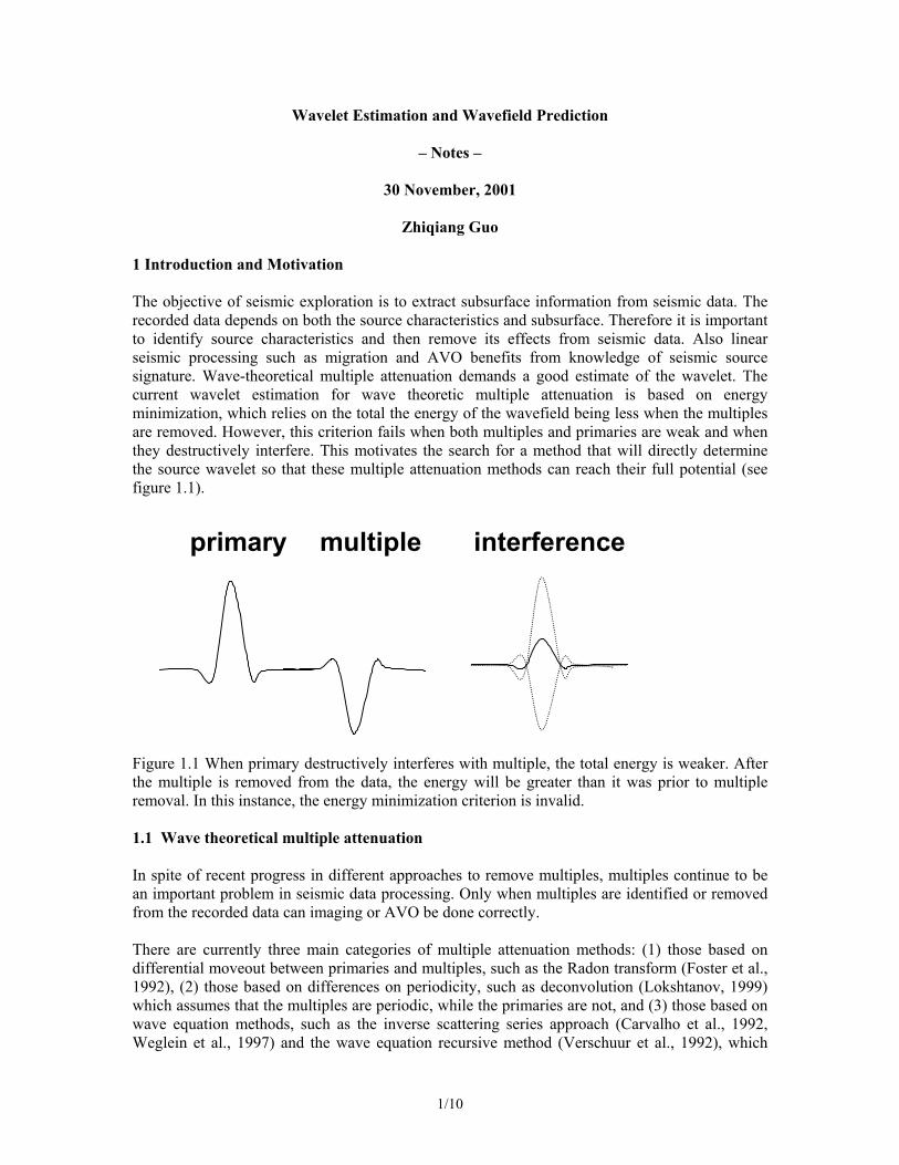
Zhiqiang Guo 1 Introduction and Motivation The objective of seismic exploration is to extract subsurface information from seismic data. The recorded data depends on both the source characteristics and subsurface. Therefore it is important to identify source characteristics and then remove its effects from seismic data. Also linear seismic processing such as migration and AVO benefits from knowledge of seismic source signature. Wave-theoretical multiple attenuation demands a good estimate of the wavelet. The current wavelet estimation for wave theoretic multiple attenuation is based on energy minimization, which relies on the total the energy of the wavefield being less when the multiples are removed. However, this criterion fails when both multiples and primaries are weak and when they destructively interfere. This motivates the search for a method that will directly determine the source wavelet so that these multiple attenuation methods can reach their full potential (see figure 1.1).

primary multiple interference

Figure 1.1 When primary destructively interferes with multiple, the total energy is weaker. After the multiple is removed from the data, the energy will be greater than it was prior to multiple removal. In this instance, the energy minimization criterion is invalid. 1.1 Wave theoretical multiple attenuation

In spite of recent progress in different approaches to remove multiples, multiples continue to be an important problem in seismic data processing. Only when multiples are identified or removed from the recorded data can imaging or AVO be done correctly. There are currently three main categories of multiple attenuation methods: (1) those based on differential moveout between primaries and multiples, such as the Radon transform (Foster et al., 1992), (2) those based on differences on periodicity, such as deconvolution (Lokshtanov, 1999) which assumes that the multiples are periodic, while the primaries are not, and (3) those based on wave equation methods, such as the inverse scattering series approach (Carvalho et al., 1992, Weglein et al., 1997) and the wave equation recursive method (Verschuur et al., 1992), which

1/10

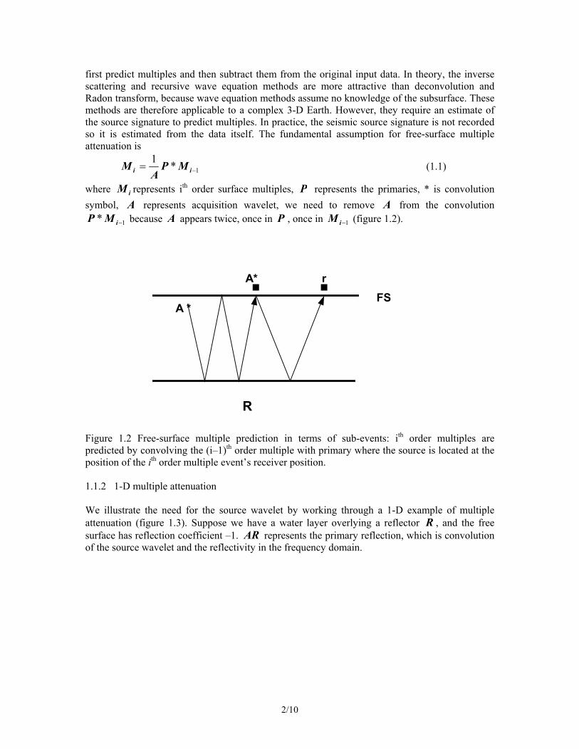
first predict multiples and then subtract them from the original input data. In theory, the inverse scattering and recursive wave equation methods are more attractive than deconvolution and Radon transform, because wave equation methods assume no knowledge of the subsurface. These methods are therefore applicable to a complex 3-D Earth. However, they require an estimate of the source signature to predict multiples. In practice, the seismic source signature is not recorded so it is estimated from the data itself. The fundamental assumption for free-surface multiple attenuation is

1*1−= ii MP

AM (1.1)

where represents iiM th order surface multiples, P represents the primaries, * is convolution symbol, A represents acquisition wavelet, we need to remove A from the convolution

because 1−i*MP A appears twice, once in P , once in (figure 1.2). 1−iM

R

A *FS

rA*

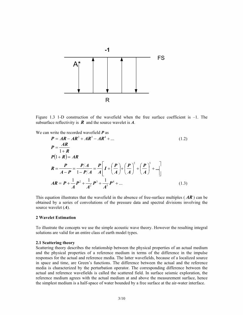
Figure 1.2 Free-surface multiple prediction in terms of sub-events: ith order multiples are predicted by convolving the (i–1)th order multiple with primary where the source is located at the position of the ith order multiple event’s receiver position. 1.1.2 1-D multiple attenuation We illustrate the need for the source wavelet by working through a 1-D example of multiple attenuation (figure 1.3). Suppose we have a water layer overlying a reflector R , and the free surface has reflection coefficient –1. AR represents the primary reflection, which is convolution of the source wavelet and the reflectivity in the frequency domain.

2/10

-1

R

A*FS

Figure 1.3 1-D construction of the wavefield when the free surface coefficient is –1. The subsurface reflectivity is R and the source wavelet is A. We can write the recorded wavefield P as

...432 +−+−= ARARARARP (1.2)

RARP+

=1

( ) ARRP =+1

+

+

+

+=

−=

−= ...

32

1 AP

AP

API

AP

APAP

PAPR

...111 43

32

2 ++++= PA

PA

PA

PAR (1.3)

This equation illustrates that the wavefield in the absence of free-surface multiples ( AR ) can be obtained by a series of convolutions of the pressure data and spectral divisions involving the source wavelet (A). 2 Wavelet Estimation To illustrate the concepts we use the simple acoustic wave theory. However the resulting integral solutions are valid for an entire class of earth model types. 2.1 Scattering theory Scattering theory describes the relationship between the physical properties of an actual medium and the physical properties of a reference medium in terms of the difference in the impulse responses for the actual and reference media. The latter wavefields, because of a localized source in space and time, are Green’s functions. The difference between the actual and the reference media is characterized by the perturbation operator. The corresponding difference between the actual and reference wavefields is called the scattered field. In surface seismic exploration, the reference medium agrees with the actual medium at and above the measurement surface, hence the simplest medium is a half-space of water bounded by a free surface at the air-water interface.

3/10

Based on scattering theory, the actual earth can be parameterized as a homogeneous velocity reference medium with embedded reflectors (figure 2.1).

Figure 2.1 The actual heterogeneous medium can be parameterized as a homogeneous velocity reference medium with embedded scattering points.

Hence

( ) ( )[ rcrc

α−= 111

02 ] (2.1)

Where is reference medium velocity, 0c ( )rα is called the index of refraction, which is used to characterize the difference between the actual and reference media, is actual medium velocity. The variable velocity acoustic wave equation in an inhomogeneous medium, with constant density and localized source in the time and spatial domain is

c

)(tA

( ) ( ) ( ) ( )020

2

202 ),,(1,, rrtA

ttrrP

rctrrP −=

∂∂

−∇ δ

Performing a temporal Fourier transform dtetrrPrrP tiωω ),,(),,( 00 ∫= the wave equation above is re-written in frequency and spatial domain as

( ) ( ) ( ) ( ) ( 002

2

02 ,,,, rrArrP

rcrrP −=+∇ δωωωω ) (2.2)

where is any point in half space, r is source location below free surface, r 0 )(ωA is the source signature, ω is angular frequency, P is the pressure field, (.)δ is a Dirac delta function, c is the actual medium velocity, we choose to characterize the velocity configuration c in term of a reference value c and a variation in scattered index

)(r)(r

0 ( )rα defined in equation (2.1). Substituting equation (2.1) into equation (2.2) and reform it to

( ) [ ] ( ) ( ) ( 0020

2

02 ,,)(1,, rrArrPr

crrP −=−+∇ δωωαωω )

( ) ( ) ( ) ( ) ( ) ( )0020

2

020

2

02 ,,,,,, rrArrPr

crrP

crrP −+=+∇ δωωαωωωω (2.3)

We can regard the first term in right-hand side of equation (2.3) as the passive source due to scattering potential ( )rα . Taken together, the two terms on the right-hand side of equation (2.3) constitute the sources that produce the wavefield ),,( 0 ωrrP . Hence equation (2.3) can be written as an integral equation using the principle of superposition.

4/10

( ) ( ) ( ) ( ) ( ) rdrrGrrArrPrc

rrPV

′′

−′+′′= ∫ ),,(,,,, ωδωωαωω 0002

0

2

0 (2.4)

where ),,( ωrrG ′0 is the Green’s function for the constant reference medium, satisfying the following equation.

( ) ( ) ( rrrrGc

rrG ′−=′+′∇ δωωω ,,,, 020

2

02 )

Furthermore equation (2.4) can be written as

( ) ( ) ( ) ( ) ( )∫∫ ′′

′′+′′−′=

VV

rdrrGrrPrc

rdrrGrrArrP ),,(,,),,(,, ωωαωωδωω 0020

2

000

Using the delta function property

VaafdrrfarV

∈=−δ∫ ,)()()(

we have

( ) ( ) ( ) ( ) rdrrGrrPrc

rrGArrPV

′′′′+= ∫ ),,(,,),,(,, ωωαωωωω 0020

2

000 (2.5)

Equation (2.5) is called the Lippmann-Schwinger integral equation and is valid for all . It can be also expressed as

r

),,(),,(),,( 0000 ωωω rrPrrPrrP s+= (2.6) where ),,()(),,( 0000 ωωω rrGArrP = (2.7)

( ) ( ) ( ) rdrrPrc

rrGrrPs ′′′′= ∫ ωαωωω ,,),,(,, 020

2

00 (2.8)

),,( 00 ωrrP represents direct waves from source r to point r , 0 ),,( 0 ωrrPs represents scattered field. The physical interpretation of equation (2.5 or 2.6) is that the total seismic wave field ),,( 0 ωrrP can be expressed as the sum of reference wave-field , the wavefield due to actual source in homogeneous velocity reference medium, and scattered field , the wavefield due to scatters (deviation from the reference medium) in a (e.g., homogeneous) velocity reference medium.

0P

sP

Now we build the Green’s function ( )ω,, rrD ′0G in a homogenous medium with a supposed source at and its corresponding mirror-imaged source r with opposite sign across free surface FS (figure 2.2), our goal is make the Green’s function satisfy the Dirichlet boundary condition on free surface.

r I

( ) ( ) ( ) ( rrrrrrGc

rrG IDD ′−−′−=′+′∇ δδωωω ,,,, 02

0

2

02 ) (2.9)

5/10

FS

MS

∗

•

• Ir

r

0rV

α

H

Figure 2.2 r is the mirror image point r across FS I

Substituting the wavefield ),,( 0 ωrrP in equation (2.3) and the Green’s function G in equation (2.9) to Green’s theorem

( )ω,, rrD ′0

( ) ( ) ( ) ( )[ ]=′∇′−′∇′′∫∫∫v

DD rrPrrGrrGrrPrd ωωωω ,,,,,,,, 02

002

0

( ) ( ) ( ) ( )

∂′∂′−

∂′∂′′∫∫ n

rrPrrGnrrGrrPrd D

D

S

ωω

ωω

,,,,,,,, 00

00 (2.10)

Then we have ( ) ( ) ( ) ( )[ ]=′∇′−′∇′′∫∫∫

v


002

0

( ) ( ) ( ) ( ) ( ) ( ) (∫∫∫

′′′−′−′−′−′

v

DI rrPrrrG

crrrrPrrrrPdr ωαωωδωδω ,,,,,,,,' 002

0

2

00 )

+ ( ) ( ) ( )[∫∫∫ −′′−′v

D rrrrGArd 00 δωω ,, ] (2.11)

We choose the integral volume V to be region between free surface (FS) and measurement surface (MS) (see figure 2.2). Furthermore, notice the third term in right hand side of equation (2.11) will be zero since the scattering potential ( )r ′α is outside of the integral V . Again, using the sifting property of the delta function, the first and second terms in right-hand side of equation (2.11) are both zero because r and its mirror image are beyond V . Hence equation (2.11) can be rewritten as

Ir

( ) ( ) ( ) ( )[ ]=′∇′−′∇′′∫∫∫v


002

0

( ) ( )ωω ,, 00 rrGA D−Combining this equation with the right hand side of equation (2.10), we obtain

6/10

( ) ( )ωω ,, 00 rrGA D− = ( ) ( ) ( ) ( )

∂′∂′−

∂′∂′′∫∫ n

rrPrrGnrrGrrPrd D

D

S

ωω

ωω

,,,,,,,, 00

00 (2.12)

Notice that both the Green’s function ( )ω,,rrGD ′0 and P are zero at the free surface (FS). Then equation above becomes:

( ) ( )ωω ,, 00 rrGA D− = ( ) ( ) ( ) ( )

∂′∂′−

∂′∂′′∫∫ n

rrPrrGnrrGrrPrd D

D

MS

ωω

ωω

,,,,,,,, 00

00

( )ωA = ( ) ( ) ( ) ( )

∂′∂′−

∂′∂′′−

∫∫ nrrPrrG

nrrGrrPrd

rrGD

D

MSD

ωω

ωω

ω,,,,,,,,

),,(0

00

000

1 (2.13)

Equation (2.13) will be used to compute the wavelet. The expression ( ) ( ωω ,, 00 rrGA D− ) is the reference wavefield ),,( 00 ωrrP

0GDD

and in the case where the actual source is in fact a superposition of notional point sources, this expression yields the source wavelet radiation pattern. Next we will describe a Green’s function that vanishes at the free surface and the measurement surface.

( ω,, 0rr )

3 Wavefield Prediction 3.1 Wavefield prediction above MS To remove the need for the normal derivative of the pressure at the measurement surface (MS) in equation (2.13), we write the wave equation in the frequency domain

( ) ( ) ( ) ( ) ( 002

2

02 rrArrP

rcrrP −′=′

′+′∇ δωωωω ,,,, ) (3.1)

Take Green’s function as following expression

( ) ( ) ( ) ( rrrrrrGc

rrG IDDDD ′−−′−=′+′∇ δδωωω ,,,, 02

0

2

02 ) (3.2)

where is chosen to be inside the region between free surface (FS) and measurement surface (MS), it is the mirror image of r across MS (Figure 3.1).

Ir

7/10

FS

MS

∗

•

• Ir

r

0r

V

α

H

Figure 3.1 Mirror image of r across the measurement surface MS inside. The volumeV is bounded by the free surface and the measurement surface, and extends to infinity laterally.

Ir

Apply Green’s theorem

( ) ( ) ( ) ( )[ ]=′∇′−′∇′′∫∫∫v

DDDD rrPrrGrrGrrPrd ωωωω ,,,,,,,, 02

002

0

( ) ( ) ( ) ( )

∂′∂′−

∂′∂′′∫∫ n

rrPrrGnrrGrrPrd DD

DD

S

ωω

ωω

,,,,,,,, 00

00

Based on equation (2.1)

( ) ( )[ ]rcrc

α−= 111

02

Substituting, we have

( ) ( ) ( ) ( ) ( ) ( ) (∫∫∫

′′′−′−′−′−′′

v

DDI rrPrrrG

crrrrPrrrrPrd ωαωωδωδω ,,,,,,,, 002

0

2

00 ) +

( ) ( ) ( )[ ]∫∫∫ −′′−′v

DD rrrrGArd 00 δωω ,,

= ( ) ( ) ( ) ( )

∂′∂′−

∂′∂′′∫∫ n

rrPrrGnrrGrrPrd DD

DD

S

ωω

ωω

,,,,,,,, 00

00 (3.3)

If we choose and scatterers r )(r ′α to be outside of the volume integral, then using the delta function property

( ) ( )[ ] ( )rfrfrrrdv

=′′−′∫∫∫ δ

the first term and second term in left hand side of equation (3.3) become ( ) ( )[ ]∫∫∫ =′−′′

v

rrrrPrd 00 δω,,

8/10

( ) ( )[ ] ( )ωδω ,,,, 00 rrPrrrrPrd Iv

I∫∫∫ =′−′′ (3.4)

Also notice the third term on the left hand side of equation (3.3) will be zero due to the fact that )(r ′α is outside of the volume integral. Hence we have

( ) ),,()(,, ωωω 000 rrGArrP DDI −− =

( ) ( ) ( ) ( )

∂′∂′−

∂′∂′′∫∫ n

rrPrrGnrrGrrPrd DD

DD

S

ωω

ωω

,,,,,,,, 00

00

We have selected the Green’s function ( )ω,, rrDD ′0

0

G to be zero on both FS and MS (see Morse and Feshbach, Chapter 7). It is assumed that 0=′ =′ FSr|)rrP ,,( ω , then

( ) ( ) ( )

∂

′∂′′=−− ∫∫ nrrGrrPrdrrGArrP

DD

MS

DDI

ωωωωω

,,,,),,()(,, 00000 (3.5)

Tan (1999) points out that is vanishingly small for typical marine survey depths of approximately 6 m and seismic frequency less than 125 Hz. Therefore, the second term on the right hand side of the equation (3.4) can be ignored in comparison with the other terms. This results in the key observation:

( ω,, rrG DD ′0 )

( ) ( ) ( )

∂

′∂′′≈− ∫∫ nrrGrrPrdrrP

DD

MSI

ωωω

,,,,,, 000 (3.6)

which can be used to predict wavefield at any point between the free surface and measurement surface using the Green’s function that satisfies the Dirichlet boundary condition on the free surface and the measurement surface.

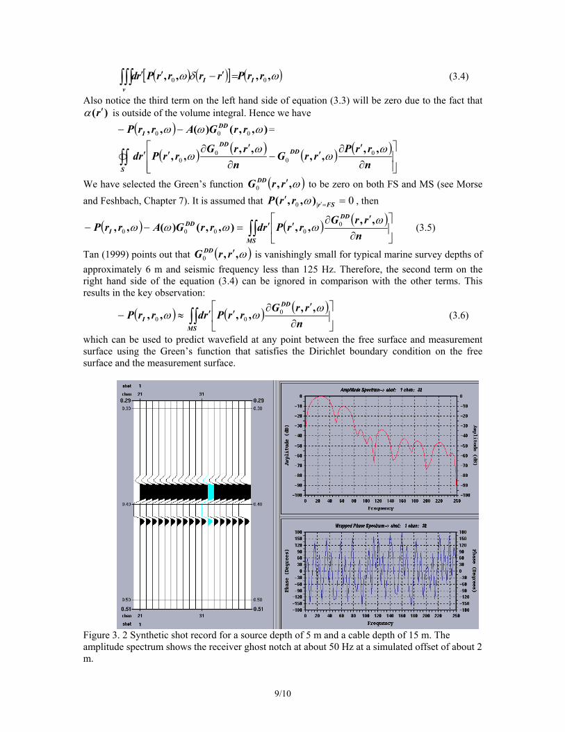
Figure 3. 2 Synthetic shot record for a source depth of 5 m and a cable depth of 15 m. The amplitude spectrum shows the receiver ghost notch at about 50 Hz at a simulated offset of about 2 m.

9/10

Figure 3.3 Predicted wavefield above the cable using equation (3.6) and the data in Figure 3.2 as input. The new cable depth is now 7 m below the free surface. The receiver ghost notch of the input data has been filled in (moved to higher frequency), and hence the bandwidth is improved. This is a preliminary but encouraging result.

Figure 3.4 Synthetic shot record for a source depth of 5 m and a cable depth of 7 m. Compare with the predicted wavefield (Figure 3.3).

10/10

A method for deghosting of towed streamer data

without spectral division and without the need for

an extra measurement

Notes

A.B. Weglein M-OSRP

S.A. Shaw, BP and M-OSRP

G.J.P. Correa, M-OSRP

Z. Guo, M-OSRP

T.H. Tan, Shell

December 4, 2001

1

1 Summary

We present a method for removing receiver ghosts from towed streamer data.The method has the following properties

1. Only pressure measurements along a cable are required.

2. There is no spectral division.

3. The cable should consist of single sensor hydrophones.

4. When the source is above the cable, then the direct wave is also re-moved.

The method is derived using the Extinction Theorem. In the limit that weevaluate our result on the measurement surface, this theory corresponds totraditional up/down separation or P-Z summation. However, in principle, itproduces the receiver deghosted data anywhere on or above the measurementsurface.

This method makes use of the speci�c property of a Green's Functionthat becomes vanishingly small for typical towed streamer depths ( 6m) andseismic frequencies (< 125 Hz).

2 Extinction Theorem for receiver deghosting

Green's Theorem statesZV

(�r2�r2�)dV =

IS

(�r�r�) � n̂ dS (1)

Consider a background medium that consists of a homogenous wholespaceof water having velocity c0. The Green's Function for this medium, G0, sat-is�es �

r2 +!2

c20

�G0(~r j~r

0;!) = Æ(~r � ~r 0) (2)

In this derivation, we will assume that our actual medium is acoustic withconstant density and variable velocity and therefore supports the wave�eldP which satis�es�

r2 +!2

c2(~r )

�P (~r j~r s;!) = A(!)Æ(~r � ~r s) (3)

1

where A(!) is the source signature.We could also write an elastic wave equation for our actual medium.Now de�ne scattering (passive) sources as follows

1

c2(~r )=

1

c20

[1� �a(~r )� �e(~r )] (4)

where �a and �e describe the scattering potentials of the air (-water inter-face) and the earth, respectively (see Fig. 1). Then we can rewrite Eq.3using Perturbation Theory

�r2 + k20

�P (~r j~r s;!)

= A(!)Æ(~r � ~r s) + k20 [�a(~r ) + �e(~r )]P (~r j~r s;!) (5)

where k0 =!c0. Rearranging this equation gives

r2P (~r j~r s;!) = A(!)Æ(~r � ~r s)� k20P (~r j~r s;!)

+ k20 [�a(~r ) + �e(~r )]P (~r j~r s;!) (6)

and from Eq.2 we have

r2G0(~r j~r0;!) = �k20G0(~r j~r

0;!) + Æ(~r � ~r 0) (7)

Substituting � = G0(~r j~r0;!) and = P (~r 0j~r s;!) in Eq.1 we have

Z~r 02V

�A(!)G0(~r j~r

0;!)Æ(~r 0 � ~r s) +G0(~r j~r0;!)k20�a(~r

0)P (~r 0j~r s;!)

+G0(~r j~r0;!)k20�e(~r

0)P (~r 0j~r s;!)� P (~r 0j~r s;!)Æ(~r � ~r 0)dV

=

I~r 02S

�G0(~r j~r

0;!)r0P (~r 0j~r s;!)� P (~r 0j~r s;!)r0G0(~r j~r

0;!)� n̂ dS

(8)

Now consider the volume, V , bounded by the surface S = S0 + SRdepicted in Fig. 1. S0 is the measurment surface, e.g., the towed streameror ocean bottom cable. We notice that �a is outside the volume and thereforedoes not contribute to the volume integral. The source location rs is alsooutside the volume so Æ(~r 0 � ~r s) = 0 for all ~r 0 in V . We also choosethe evaluation point r to be outside the volume by placing it above themeasurement surface. Hence, Æ(~r � ~r 0) = 0 for all ~r 0 in V . Then, if wemake use of the causal Green's Function G+

0and apply the Sommerfeld

2

radiation condition such that contributions from the surface SR becomezero as R!1, Eq. 8 becomes

Z~r 02V

G+0(~r j~r 0;!)k20�e(~r

0)P (~r 0j~r s;!)dV

=

Z~r 02S0

�G+0(~r j~r 0;!)r0P (~r 0j~r s;!)� P (~r 0j~r s;!)r

0G+0(~r j~r 0;!)

� n̂ dS0

(9)

The left-hand side of Eq. 9 is the receiver-deghosted scattered �eld, Prdg.The volume integral contains no interactions with �a; it can be interpretedas an in�nite sum of propagations from the source and the free surfacethrough the actual medium (P ), scattering in the Earth (k20�e), followed bypropagation in water back to the receivers (G+

0). Prdg is only the upgoing

portion of the total �eld. In addition, Prdg also has the direct wave removed,meaning that it is the scattered �eld. This is evident because the direct wavehas no interactions with the Earth and so is not represented by this integral.This property is important in shallow water areas, where the direct waveinterferes with the re ection events and therefore is diÆcult to mute.

Equation 9 is a manifestation of the Extinction Theorem. We haveextinguished the contribution to the total �eld that was due to the scatteringsources above the measurement surface by choosing our output point (~r ) inthat region. In the limit that we evaluate Prdg on the measurement surface,this theory describes conventional up-down separation, sometimes call P-Zsummation. In the wavenumber domain, the surface integral is a weightedsum of the pressure measurements and the vertical component of particlevelocity.

To calculate Prdg, we evaluate the surface integral on the right-handside of Eq. 9. This requires the measured total pressure data and its normalderivative. Assuming that we know the acoustic properties of water, we canstraightfowardly calculate the Green's function and its normal derivative.Furthermore, if we were able to predict the total wave�eld above the mea-surement surface, then we could calculate its normal derivative, rather thanrequire its measurement.

3

3 Eliminating the need to measure the normal

derivative

Tan (1999) points out that, for typical streamer depths (� 6m) and seismicfrequencies (< 125 Hz), the following equation well-approximates the totalwave�eld above the cable

P (~r 0j~r s;!) �

Z~r 002S0

�P (~r 00j~r s;!)r

00GDD0 (~r 0j~r 00;!)

� n̂ dS0 (10)

where GDD0 is a Green's function that vanishes (equals zero) at the free

surface and on the measurement surface (Tan 1999, Osen et al. 1998).Weglein et al. (2000) propose that, since Eq. 10 gives us an in�nite numberof estimates of the total wave�eld above the cable, we can predict the �eld attwo or more depths and calculate its normal derivative. In 2-D, the verticalderivative can be expressed using Eq. 10 as

@

@z0P (x0; z0jxs; zs;!) �Z

1

�1

P (x00; zcjxs; zs;!)

�@2

@z0@z00GDD0 (x0; z0jx00; z00;!)

�z00=zc

z=zc��

dx00 (11)

where zc is the cable depth and � is a small positive number. As � ! 0+,Eq. 11 is the vertical derivative of the total pressure �eld on the cable.Rewriting Eq. 9 in 2-D and then substituting in Eq. 11, we have

Prdg(x; zjxs; zs;!) �

Z1

�1

fG+

0(x; zjx0; zc;!)

Z1

�1

P (x00; zcjxs; zs;!)

�@2

@z0@z00GDD0 (x0; z0jx00; z00;!)

�z00=zc

z=zc��

dx00

�P (x0; zcjxs; zs;!)@

@z0G+0(x; zjx0; z0;!)

�dx0 (12)

This is an expression for the upgoing wave�eld in terms of only pressuremeasurements on the cable, and analytic reference Green's Functions.

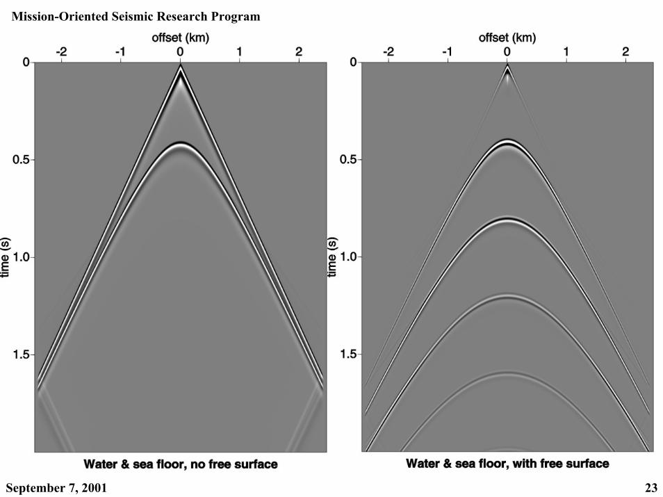
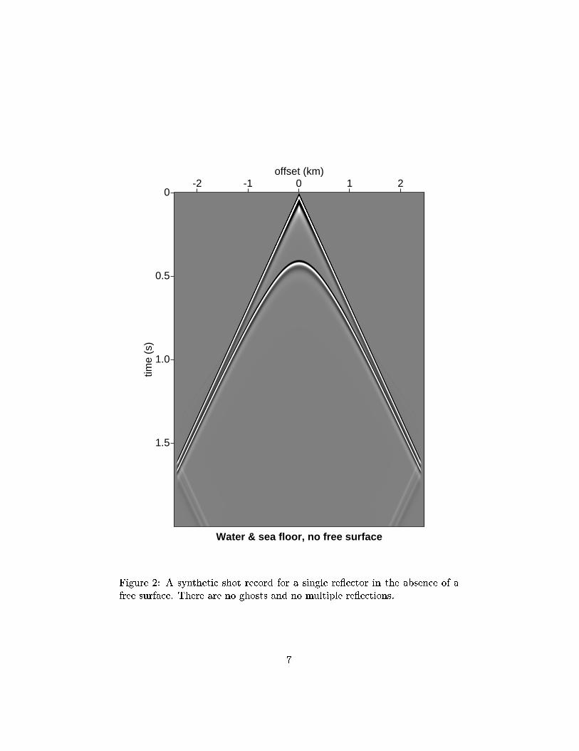
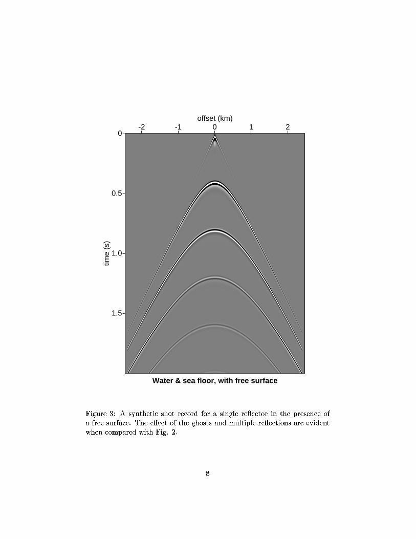
We propose to code the algorithm for Prdg (Eq. 12) and test its e�ective-ness by �rst applying it to synthetic data. For example, Figs. 2 and 3 havebeen prepared for this purpose. We can clearly see the e�ect that the freesurface has on the sea oor re ector by comparing these two shot records.When we have completed this test, we will test the algorithm on �eld data.Experience has shown that these methods require a good recording of the

4

direct wave. This is achievable with single sensor data. The typical record-ing arrays are designed to dampen the direct wave and to emphasize theupgoing waves. This proved to be an impediment to implementing previ-ous wavelet estimation methods (Weglein and Secrest, 1990) that were alsoderived using Extinction Theorem.

4 Discussion

The sensitivity in traditional deghosting arises from using the boundarycondition P (z0 = 0) and the measurement P (z0 = zc). Using P (z

0 = zc) and@P@z0 (z

0 = zc) avoids the spectral division. The Extinction Theorem, and thecon uence of depths of cable and f < 125 Hz, combine to allow an algorithmthat requires only measurements P (z0 = zc) to receiver deghost the data.

It is instructive to ask whether we can treat the free-surface as a sourceand use the Extintion Theorem to remove all its e�ects, i.e., ghosts and freesurface multiples. The answer to this question is no for multiples, but yesfor receiver ghosts. The Extinction Theorem will eliminate all events whoselast interaction was on the side of the measurement surface that you chooseto evaluate the wave�eld. Free surface multiples have more complicatedinteractions with scattering sources �a and �e.

5

S0

SR

rrs

V�e

�a

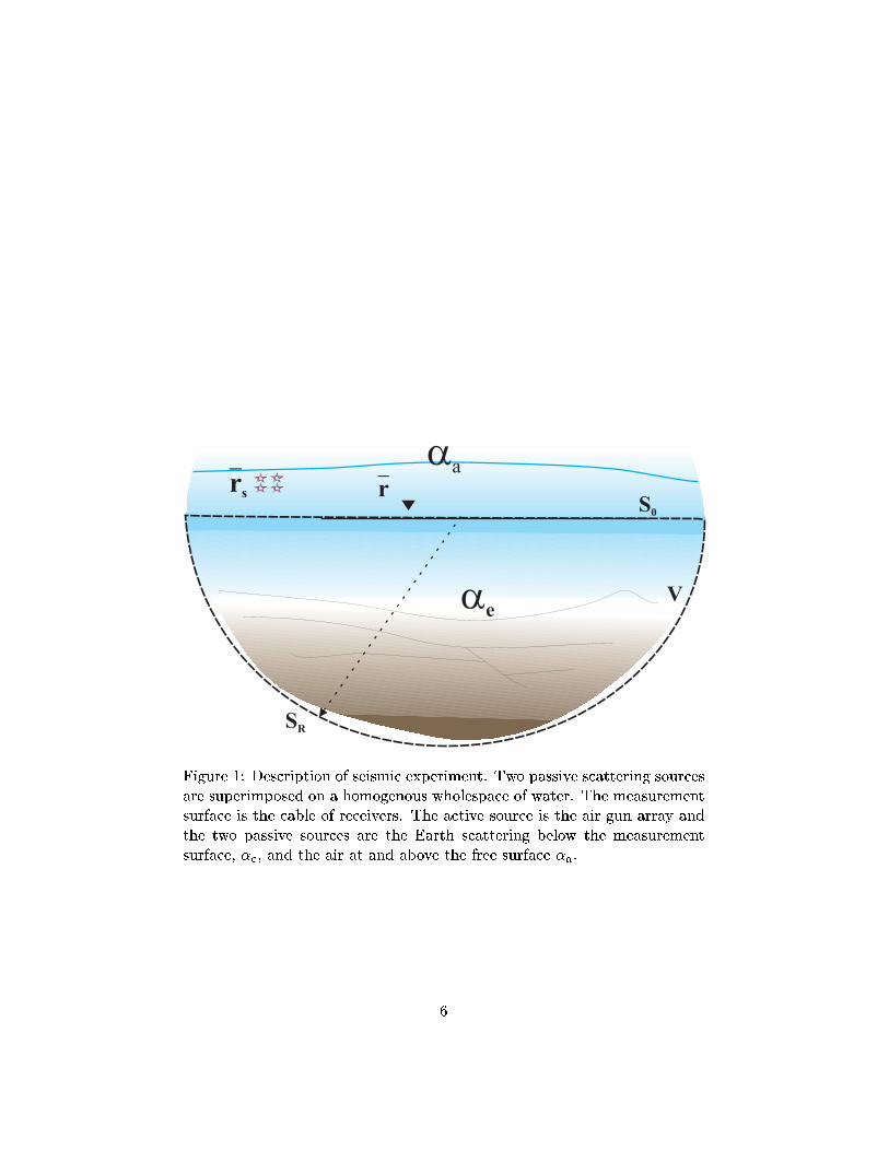
Figure 1: Description of seismic experiment. Two passive scattering sourcesare superimposed on a homogenous wholespace of water. The measurementsurface is the cable of receivers. The active source is the air gun array andthe two passive sources are the Earth scattering below the measurementsurface, �e, and the air at and above the free surface �a.

6

0

0.5

1.0

1.5

time

(s)

-2 -1 0 1 2offset (km)

Water & sea floor, no free surface

Figure 2: A synthetic shot record for a single re ector in the absence of afree surface. There are no ghosts and no multiple re ections.

7

0

0.5

1.0

1.5

time

(s)

-2 -1 0 1 2offset (km)

Water & sea floor, with free surface

Figure 3: A synthetic shot record for a single re ector in the presence ofa free surface. The e�ect of the ghosts and multiple re ections are evidentwhen compared with Fig. 2.

8

Notes

A. B. Weglein

December 3, 2001

1 Directly computing the wavelet, radiation pat-

tern and deghosted data from a single shot

record

The wave�eld P can be computed above the cable from P along the cable (H.Tan 1999).

P (x; z; xs; zs;!) =

ZP (x0; zc; xs; zs; !)

�@GDD

0 (x; z; x0; z0; !)

@z0

�z0=zc

dx0 (1)

where zc = zcable:

The vertical derivative of the measured wave�eld can be computed by taking@@z

of (1) and evaluating at z = zc � � (slightly above the cable: +z pointsdownward):

lim�!0+

�@P

@z(x; z; xs; zs;!

�z=zc��

(2)

= lim�!0+

ZP (x0; zc; xs; zs;!)

�@2GDD

0 (x; z; x0; z0; !)

@z@z0

�z0=zcz=zc��

dx0:

The extinction theorem allows an integral that involves P and @P@z

along thecable to compute P0 for z > zc and �Ps for z < zc (see Weglein and Secrest1990):

�P0(x; z; xs; zs;!) z < zcPs(x; z; xs; zs;!) z > zc

�= �

ZfP (x0; zc; xs; zs;!)

�@GD

0 (x; z; x0; z0; !)

@z0

�z0=zc

(3)

�

�@P (x0; z0; xs; zs;!)

@z0

�z0=zc

GD0 (x; z; x

0; zc; !)gdx0

Evaluate (2) at

(x; z; xs; zs) �! lim�!0+

(x; z; xs; zs)z=zc�� (4)

1

to �nd

lim�!0+

�@P (x0; z0; xs; zs; !)

@z0

�z0=zc��

(5)

= lim�!0+


�@2GDD

0 (x0; z0; x00; z00; !)

@z0@z00

�z0=zc��z00=zc

dx00

and substituting (5) into (3), the right hand member of equation (3) becomesZ (P (x0; zc; xs; zs;!)

�@GD

0 (x; z; x0; zc; !)

@z0

�z0=zc

)dx0 (6)

� lim�!0+

f


@2GDD0 (x0; z0; x00; z00; !)

@z0@z00GD0 (x; z; x

0; z0; !)dx00dx0gz0=zc��z00=zc

:

We can eliminate the need for @P@z0

by using equation (2) and the fact that

P and @P@z0

are continuous functions in space so that the limit from above thecable can be used for the value on the cable

lim�!0+

�@P (�!r 0;�!rs ;!)

@z0

�z0=zc��

=@P (x0; zc;�!rs ;!)

@z0: (7)

We have�+P0(x; z; xs; zs;!) for z below zc�Ps(x; z; xs; zs;!) for z above zc

�

= �

ZdxgP (xg; zc; xs; zs;!)f

�@GD

0 (x; z; xg; z0;!)

@z0

�z0=zc

� lim�!0+

Z 24�@2GDD

0 (x0; z0; xg; z00; !)

@z0@z00


GD0 (x; z; x

0; zc; !)

35 dx0g(8)

The G0; GD0 ; and GDD

0 are all causal in these extinction theorem applica-tions.

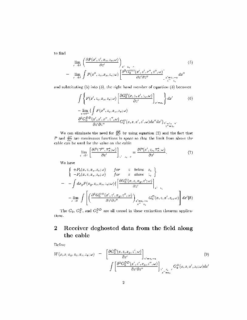
2 Receiver deghosted data from the �eld along

the cable

De�ne

W (x; z; xg; zc; xs; zs;!) �

�@GD

0 (x; z; xg; z0;!)

@z0

�z0=zc��

(9)

�

Z �@2GDD

0 (x0; z0; xg; z00; !)

@z0@z00


GD0 (x; z; x

0; zc;!)dx0

2

[GD0 and GDD

0 are analytic functions (see Morse and Feshbach, Chapter 7)].RESULT: A single weighted integral over xg of the data on the cable for a

single shot record,ZP (xg; zc; xs; zs;!)W (x; z; xg; zc; xs; zs;!)dxg (10)

produces (for that shot record) the reference wave�eld, P0; (wavelet and radia-tion pattern) for all (x; z) with z > zc (i.e. at any point below the cable) andthe scattered �eld (actually �Ps) for all (x; z) with z < zc (i.e. at any pointabove the cable). When the reference �eld, P0; is due to a localized source,then P0 = A(!)G+

0 (�!r ;�!rs ;!) where A (!) is the source signature (phase and

amplitude) and is directly computable from the data recorded with the cable foreach shot record.

SIGNIFICANCE: The total measured wave�eld, P; integrated over thecable produces the amplitude and phase of the wavelet (and source radiationpattern) for that shot record without a second cable, or well, or 1-D, or statisticalassumptions.

There is a rejuvenated interest in estimating the source signature (and pat-tern) for free surface and internal multiple attenuation. Current methods forestimating the wavelet (for those applications) can keep the underlying powerof the demultiple techniques (e.g., for separating interfering primary and multi-ple events) from reaching their full potential. This wavelet estimation methodmakes no assumption that is at cross purposes with the underlying capabilityof the inverse scattering demultiple methods.

Deghosting: We start by observing that for each shot-record, the receiverdeghosted data can be computed directly from the measured total �eld, P; andits normal derivative dP

dz0along the cable.

P deghosted(�!r ;�!rs ;!) =

Zz0=zc

fP (�!r 0;�!rs ;!)@G+

0 (�!r ;�!r 0;!)

@z0(11)

�G+0 (�!r ;�!r 0;!)

@P (�!r 0;�!rs ;!)

@z0gdx0

whereG+

0 is the whole-space causal Green's function (in 3-D)G+

0 = � 1

4�eikj

�!r ��!r0j

j�!r ��!r 0j

and the evaluation point �!r is above the cable, i.e. z > zc: We have

P deghosted =

ZfP (x0; zc; xs; zs;!)

�@G0(x; z; x

0; z0;!)

@z0

�z0=zc

(12)

�G0(x; z; x0; zc;!) lim

�!0+


�@2GDD

0 (x0; z; x00; z00;!)

@z0@z00


dx00gdx0:

3

Substituting @P@z0

from equation (2) in equation (13) we �nd

P deghosted(x; z; xs; zs;!) =

ZdxgP (xg; zc; xs; zs;!)f

�@G0(x; z; xg; z

0;!)

@z0

�z0=zc

� lim�!0+

Z[

�@2GDD

0 (x0; z0; xg; z00; !)

@z0@z00


(13)

G0(x; z; x0; zc;!)]dx

0g:

Equation (14) produces deghosted P for all points above the cable.

3 Summary

The new results of this section derive from an evolution of ideas, Weglein andSecrest (1990), H. Tan (1992), Osen et al (1998), H. Tan (1999), Weglein, Tanet al. (2000) that provide the opportunity to estimate the wavelet and deghostyour data from an integral over your shot record without: sensitive divisionoperations, the need for either an extra towed streamer or well information, orany �nite di�erence or Taylor series approximations.

The wavelet, A(!), for each shot record is

A(!) =

RP (xg; zc; xs; zs;!)W1(x; z; xg; zc; xs; zs;!)dxg

G0(x; z; xs; zs;!)(14)

for any (x; z) below the cable. This freedom to choose the evaluation point(x; z) provides (in practice) a plethora of estimates for A(!): Delima et al.(1990) exploited this freedom to provide robust estimates of A(!) when P andPn were measured. Here equation (15) provides a similar suit of estimates forA(!) with only P on the cable.

P deghosted(x; z; xs; zs;!) =

ZP (xg; zc; xs; zs;!)W2(x; z; xg; zc; xs; zs;!)dxg

(15)

for any (x; z) above the cable.W1 andW2 are given by equation (7) or what equation (7) becomes when GD

0

is replaced by G0; namely equation 14, for wavelet or deghosting application.All of these extinction theorem applications require single sensor data, i.e. ameasurement of P that retains both Ps (re ection data) and P0 the referencewave�eld.

4

Copyright 2000, Offshore Technology Conference This paper was prepared for presentation at the 2000 Offshore Technology Conference held in Houston, Texas, 1–4 May 2000. This paper was selected for presentation by the OTC Program Committee following review of information contained in an abstract submitted by the author(s). Contents of the paper, as presented, have not been reviewed by the Offshore Technology Conference and are subject to correction by the author(s). The material, as presented, does not necessarily reflect any position of the Offshore Technology Conference or its officers. Electronic reproduction, distribution, or storage of any part of this paper for commercial purposes without the written consent of the Offshore Technology Conference is prohibited. Permission to reproduce in print is restricted to an abstract of not more than 300 words; illustrations may not be copied. The abstract must contain conspicuous acknowledgment of where and by whom the paper was presented.

Abstract The inverse scattering series represents the only direct multidimensional inversion procedure. The directness of the method (towards a single objective) implies a purposefulness and focus. If the objective is viewed as being achieved through an ordered sequence of steps, we can then imagine that these steps themselves reside in the algorithm. The logic behind the resulting free-surface and internal multiple attenuation algorithms is revisited and an informal comparison with the evolution of the feedback method is presented. The inverse scattering multiple attenuation algorithms are illustrated using field-data examples.

Introduction The inverse scattering method for attenuating free-surface and internal multiples (Ref. 1, Ref. 2, Ref. 3) provides a unique set of algorithms for the removal of all free-surface and internal multiples with absolutely no subsurface information, interpretive intervention, iteration, updating, muting, or velocity or event picking. These algorithms derive from identifying terms (and portions of terms) of the multidimensional inverse series for seismic data (Ref. 4) that carry out specific tasks, within the overall inversion process, in a purposeful and direct manner. This concept of associating certain terms (and subseries) with task-separated inverse processes allows great benefit to derive from reaching one (or more) of these goals under circumstances when all of these objectives are not achievable. Further, the fact that each term has a well-defined specific function, within this four distinct task separated inversion framework, allows the prediction of the effect of different portions of the series – independent of

the nature of the target. For example, the individual terms in the free-surface demultiple subseries each eliminate a different specific order of free-surface multiple – completely and totally independent of the nature of the earth. These terms carry out their assigned purpose not only independent of the nature of the earth’s structure and lithology, but also independent of whether the earth is acoustic, elastic or anelastic. A recent set of papers (Ref. 5, Ref. 6) provided synthetic data tests as an empirical comparison of these inverse scattering free-surface and internal multiple methods and the feedback method pioneered by Berkhout (Ref. 7) and developed by Verschuur et al. (Ref. 8). References (5) and (6) are comparison papers and mainly consist of numerical and synthetic data examples. One objective of the current paper is to continue this analysis and synthesis. Scattering theory Scattering theory is a form of perturbation theory. It relates the actual impulse response, G, and the reference impulse response, G0, to the difference between the actual and reference media, which is characterized by the operator, V. G0 and G satisfy the differential equations

δ=00GL (1)

δ=LG (2) where L0, L are the differential operators describing reference and actual propagation, δ represents an impulsive source, and VLL =−0 (3). The fundamental relationship between G, G0 and V is VGGGG 00 += (4). The forward problem starts with G0 and V and produces G; the inverse problem starts with G0 and measurements of G (on a surface outside of V) to determine V.

OTC 12011

Wave Theoretic Approaches to Multiple Attenuation: Concepts, Status, Open Issues, and Plans: Part II A. B. Weglein, K. H. Matson, ARCO E&P Technology, and A. J. Berkhout, Delft University of Technology

2 WEGLEIN, MATSON AND BERKHOUT OTC 12011

The forward problem can be represented by a series from equation (4) K+++= 000000 VGVGGVGGGG (5) and the latter can be represented as a feedback process with a series of n repeated applications of (G0V)n acting to the left of G0. The scattered field, ψs, is defined as the difference between G and G0. The inverse series constructs V as a series in orders of the measured data, D, where D=(ψs)m and (ψs)m represents the values of the scattered field ψs on the measurement surface where the sources and receivers reside. The inverse series for V is K++= 21 VVV (6) where Vn is the portion of V that is n-th order in D. Substitution of (6) into (5) evaluated on the measurement surface, and matching terms of equal order in the data gives mGVGD )( 010= (7a)

mm GVGVGGVG )()(0 01010020 += (7b)

Lmmm GVGVGGVGVGGVG )()()(0 0102002010030 ++= mGVGVGVG )( 0101010+ (7c)

M Equation (7a) allows us to solve for V1 from D and G0; (7b) allows us to solve for V2 from V1 and G0; and (7c) allows us to solve for V3 in terms of V1, V2 and G0. Hence, the construction of the entire series is given in an explicit step-by-step manner directly in terms of D and G0. Consider the ordered sequence of tasks within the process of inversion as (1) eliminate free-surface multiples (2) eliminate internal multiples (3) transform primaries in time to the imaged reflectivity in

space, and (4) invert these imaged primaries to predict the relative

changes in earth mechanical properties at the reflector. If we imagine that inversion consists of these tasks and that the construction of V is synonymous with inversion, then it follows that the four tasks reside within the construction of V. Since V is constructed from only measured data and G0 through equations (7), it then follows that each task is achievable from operations only involving the measured data and the reference Green’s function, G0. The specific subseries of equation (6) that attenuate free-surface and internal multiples are described in detail in Ref. 2 and the references contained therein.

A priori information and the reference medium The choice of reference medium (and the concomitant need for a priori information) depends on the particular inversion task you are considering, the level of reference information that allows that task-specific subseries to be useful (i.e., convergent or at least asymptotic), and the availability of reliable a priori information at that particular point in the sequence of inversion tasks. For example, prior to carrying out the tasks of multiple attenuation, it is more difficult to achieve a reliable estimate of background velocity than afterwards. In general, the simplest reference medium that satisfies the criteria listed above is the model of choice. For free-surface multiple elimination, the reference medium is a half-space of water bounded by a free-surface at the air-water boundary. The internal multiple subseries uses a whole-space of water as the reference medium. Hence, absolutely no a priori information below the measurement level is required for either the free-surface or internal multiple subseries. The reference Green’s function, G = G0

d+ G0FS for the half-

space of water bounded by a free surface at the air-water boundary is illustrated in Fig. 1. G0

d is the causal whole space Green’s function and G0

FS is the extra term in G0 due to the presence of the free surface. G0

FS can be interpreted as the response of a negative mirror-image of the actual source across the free surface: the reference Green’s function G = G0

d+ G0FS vanishes at the free surface.

The role of G0

FS in the forward series (5) is to create all of the extra events that owe their existence to the presence of the free surface. Its role in the inverse series (6) (and (7)) is to perform all of the extra inversion tasks that arise due to reflection data containing free-surface generated events (ghosts and free-surface multiples). Free-surface algorithms The feedback method for free-surface multiple attenuation describes a very similar algorithm as the inverse scattering series for free-surface multiples. The difference resides in the fact that the inverse scattering free-surface method (Refs. 1 and 2) accounts for the actual source in the water column whereas the feedback method corresponds to a vertical dipole of the actual source. However, the free-surface event generating and removing mechanism are identical and G0

FS = W+R0

−W− where W+ is the upward propagation, R0− is the

downward reflection at the free surface and W− is the downward propagation. This relates key ingredients of the inverse scattering and feedback methods for free-surface multiples and explains the similarity of their respective free-surface algorithms. Internal multiple algorithms The inverse scattering method for internal multiples corresponds to a subseries of the series for V that

OTC 12011 WAVE THEORETIC APPROACHES TO MULTIPLE ATTENUATION: CONCEPTS, SATUS, OPEN ISSUES, AND PLANS: PART II 3

automatically eliminates all internal multiples starting with data D (consisting of primaries and internal multiples) and the whole-space Green’s function for water, G0

d. The first term in that elimination series represents the attenuation of all first order internal multiples, independent of (and oblivious to) the location of the reflections that generate the upward and downward reflections. It predicts the exact time of all internal multiples and well-approximates the amplitude of internal multiples of an entire p-wave history. The arrival time of internal multiples with one or more shear-wave leg is also predicted precisely but the predicted amplitude of these converted wave internal multiples is less accurate than for the corresponding p-waves. The feedback method (Ref. 6 and Ref. 7) for internal multiples was originally formulated as basically a sequence that repeats the free-surface program by locating and defining the structure and reflection properties of the ocean bottom and subsequently reflectors below. It then removes those events that have their shallowest downward reflections at the specified reflector. This feedback program is in effect a stripping technique and requires accurate knowledge of the overburden above the reflector to allow for both precise spatial location and amplitudes of reflection (as a function of angle). The development of common-focal-point (CFP) time imaging concepts (as an intermediate step preceding imaging at depth) caused the original depth imaging of the feedback internal multiple algorithm to be examined and to evolve into a CFP time image form, for the identified reflector where a shallowest downward reflector occurs. The latter time images do not require an accurate overburden model and the resulting forms begin to emulate characteristics of the first term of the inverse scattering series for internal multiple attenuation. A different implementation of the feedback method is described in Ref. 9. The analysis and comparison of this recently evolved form of the feedback method for internal multiples and its relationship to the first term of the inverse scattering procedure continues. For achieving goals significantly beyond current internal multiple attenuation capability and moving towards internal multiple elimination, the feedback and inverse scattering methodologies are currently on two totally different trajectories. The feedback method returns to its original program of determining the velocity model of the overburden (using, e.g., one-way tomography) and depth imaging, whereas the inverse series goes to higher terms in the internal multiple removal series that only depend on D and G0, and, hence, avoids the need for the velocity or depth model. We anticipate that there will be circumstances for which either one or the other (or some combination) of these approaches for internal multiple elimination will be the method of choice. Field data example In this section, we illustrate the application of free-surface and internal multiple attenuation to a field data example. These

data are acquired in an area with a relatively shallow water bottom and a number of high amplitude reflectors at depth. The first step is to remove the free-surface multiples in preparation for internal multiple attenuation. To do this, we first we applied predictive deconvolution in the tau-p domain to attenuate the short period water-bottom and peg-leg multiples. Since we were unable to adequately estimate the water-bottom reflection in the near-offset range, we did not use the inverse scattering free-surface approach to attenuate these multiples. However, we did use this latter method to attenuate the longer period multiples associated with the deeper high amplitude reflectors. A Radon demultiple filter was then applied to further attenuate any residual multiples. In Fig. 2, we show a near-offset gather of the data before and after the application of the multiple attenuation flow described above.

After the free-surface multiples have been sufficiently removed, the data are ready for internal multiple attenuation. Since the data requirements for internal multiple attenuation are the same as for free-surface multiples, no additional data interpolation or extrapolation is required at this stage. To get an idea of the location and severity of the internal multiples, we stack the data and compute a 1D post-stack internal multiple estimate. The first panel in Fig. 3 shows the stacked section after prestack free-surface multiple removal. The second panel in this figure shows the 1D post-stack internal multiple estimate. Note the correlation between the predicted dipping internal multiples and the dipping events in the input data. Usually the 1D estimate is not suitable for subtraction since the timing and amplitudes are in error. In this case, we were successful at attenuating the predicted internal multiples using an adaptive subtraction scheme. Judicious use of adaptive subtraction is required to avoid damaging primary reflections – particularly in the case of internal multiple attenuation.

The next step is to compute an internal multiple estimate using the 2D pre-stack algorithm. While more costly than the 1D estimate, the 2D estimate has the benefit of being able to attenuate internal multiples on pre-stack gathers in preparation for AVO analysis. In addition, the amplitude and timing of the events is more accurate in 2D thus enabling a more reliable subtraction. The first panel in Fig. 4 shows a common offset gather (offset = 1000 m) of the prestack data after free-surface demultiple. The second panel shows the 2D prestack internal multiple estimate for this same offset. Again we observe a good correlation between the predicted multiples and dipping events on the input data. The third panel shows the results after adaptively subtracting the predicted internal multiples from the input data. Conclusion The inverse scattering series for attenuating free-surface and internal multiples are specifically designed for deep-water and/or complex multidimensional subsurfaces where one dimensional or moveout-trajectory assumptions are violated and where it would be prudent to avoid velocity picking, event


identification or interpretive intervention. In this paper, we revisited the logic-train behind these algorithms and continued our discussion and analysis – comparing the current and anticipated future directions of inverse scattering methods with the feedback approach. Field-data examples exemplify the inverse scattering algorithm. Acknowledgements The authors would like to thank ARCO management for providing an environment that is conducive to this long-term high impact research activity. In particular, we appreciate the constant encouragement and strong support of James D. Robertson and Dodd DeCamp. Useful conversations with Eric Verschuur, Panos Kalamis, Ray Ergas and Helmet Jakubowicz are acknowledged. The support of Delphi consortium sponsors is much appreciated. Simon Shaw is thanked for insightful discussions and for helping prepare the manuscript. References 1. Carvalho, P.M., Free-surface multiple elimination method based

on nonlinear inversion of seismic data: Ph.D. thesis, Universidade Federal da Bahia, Brazil (1992), (in Portuguese).

2. Weglein, A. B., Gasparotto, F. A., Carvalho, P. M., and Stolt, R. H., “Inverse scattering series method for attenuating multiples in

seismic data,” Geophysics (1997), 62, no. 6, 1975–1989. 3. Araujo, F.V., Weglein, A.B., Carvalho, P.M., and Stolt, R.H.,:

“Inverse scattering series for multiple attenuation: an example with surface and internal multiples,” 64th Ann. Internat. Mtg., Soc. Expl. Geophys., Exp. Abstracts (1994), 1039–1041.

4. Weglein, A. B., Boyse, W.E., and Anderson, J.E., “Obtaining three dimensional velocity information directly from reflection seismic data; an inverse scattering formalism,” Geophysics (1981), 46, no. 8.

5. Matson, K.H., Corrigan, D., Weglein, A.B., Young, C.Y.: “Inverse scattering internal multiple attenuation: results from complex synthetic and field data examples,” 69th Ann. Internat. Mtg., Soc. Expl. Geoph., Expanded abstracts (1999), 1060–1063.

6. Verschuur, D.J., Berkhout, A.J., Matson, K.H., Weglein, A.B., and Young, C.Y.: “Comparing the interface and point scatterer methods for attenuating internal multiples: a study with synthetic data – part I,” 68th Ann. Internat. Mtg., Soc. Expl. Geoph, Expanded abstracts (1998), 1519–1522.

7. Berkhout, A.J.: Seismic migration, imaging of acoustic energy by wave field extrapolation, a: theoretical aspects, Elsevier (1982).

8. Verschuur, D.J., Berkhout, A.J., and Wapenaar, C.P.A., “Adaptive surface-related multiple elimination,” Geophysics (1992), 57, 1166–1177.

9. Jakubowicz, H.,: “Wave equation prediction and removal of interbed multiples,” 68th Ann. Internat. Mtg., Soc. Expl. Geoph., Expanded abstracts (1998), 1527–1530.

OTC 12011 WAVE THEORETIC APPROACHES TO MULTIPLE ATTENUATION: CONCEPTS, SATUS, OPEN ISSUES, AND PLANS: PART II 5

G 0F S

G 0= G 0

d+ G 0FS

G 0d

* ∇∇∇∇

Fig. 1. The reference Green’s function, G0 for the free-surface multiple attenuation subseries. G0

d is the point to point propagation whole-space causal Green’s function, and G0

FS is the extra portion of G0 due to the presence of the free surface.

Data before free-surface demultiple

Data after free-surfacedemultiple

Free-surface multiples

Fig 2. Pre-stack free-surface multiple attenuation example. The first panel shows a common-offset gather (offset=1000m) before free-surface multiple attenuation. The second panel shows these data after tau-p predictive deconvolution, Inverse Scattering free-surface demultiple, and Radon demultiple. (Seismic data come from a non-exclusive survey owned by Geco-Prakla. Permission to use these data is gratefully acknowledged.)


Fig. 3. Post-stack internal multiple attenuation example. The first panel shows a stacked section after pre-stack free-surface multiple attenuation and Radon demultiple. The second panel shows the 1D post-stack internal multiple estimate computed using the stack in the first panel. The third panel shows the stack in the first panel after adaptive subtraction of the estimated internal multiples in the second panel. (Seismic data come from a non-exclusive survey owned by Geco-Prakla. Permission to use these data is gratefully acknowledged.)

Fig. 4. Pre-stack internal multiple attenuation example. The first panel shows a common offset gather (offset = 1000 ft) after pre-stack free-surface multiple attenuation and Radon demultiple. The second panel shows the 2D pre-stack internal multiple for this same offset. The third panel shows the common offset data in the first panel after adaptive subtraction of the estimated internal multiples in the second panel. (Seismic data come from a non-exclusive survey owned by Geco-Prakla. Permission to use these data is gratefully acknowledged.)

Data afterfree-surfacedemultiple

1D post-stackinternal multipleestimate

Data after internalmultiple adaptivesubtraction

internalmultiples

Common offsetgather after free-surface demultiple

2D pre-stackinternal multipleestimate

Common offset gatherafter internal multipleadaptive subtraction

internalmultiples internal

multiples

Presented at the 7th International Congress of SBGf, Salvador, Brazil (November, 2001) The inverse-scattering sub-series for the removal of free-surface and internal multiples: Status, open issues and plans A. B. Weglein (University of Houston, [email protected]) Introduction The industry trend to deepwater has raised the bar on seismic effectiveness due to a confluence of higher cost and technical challenges. Imaging beneath complex overburdens, e.g., salt, basalt, or karsted sediments, are high economic priority for hydrocarbon exploration and production and represent technical challenges without an immediately available effective response. A prerequisite for the imaging of primaries is the removal of multiples. Traditional multiple elimination techniques typically assume a 1-D earth, or periodicity of multiples, or move-out differences, or they require: velocity analysis, or interpretive intervention, or event picking. However, the level of technical challenge represented by the types of plays described above cause traditional methods to bump-up hard against their assumptions with a concomitant degradation or cessation of effectiveness. A response to the challenge The inverse-scattering multiple attenuating sub-series for free-surface and internal multiples is a direct response to this tough and important challenge. The sub-series for attenuating free-surface and internal multiples (Weglein et al. 1997, Carvalho et al. 1992, Araujo et al. 1994, Matson and Weglein 1996, Coates and Weglein 1996) were described and exemplified for towed streamer and multi-component ocean bottom and on-shore data. These multiple attenuation sub-series have excellent convergence properties, assume absolutely no information concerning the subsurface, require no velocity analysis, no event picking, nor interpretive intervention, and they have demonstrated effectiveness on field data (Carvalho et al 1992, Carvalho and Weglein 1994, Matson et al. 1999). Imagine predicting and subtracting all the multiples from a salt body, while preserving all primaries, with no information about the salt structure, nor what is above the salt, i.e., no velocity, nor any other cause or influence on these multiples. Many considered this absolutely impossible in 1990, considered it somewhat understandable by 1997, and today it is considered eminently reasonable, when production

strength codes routinely apply those algorithms and fulfill that promise. Another wave-theoretical technique, the feedback method, was pioneered by Berkhout (1982) and developed by Verschuur et al. (1992) and these two methodologies were compared (e.g., Berkhout et al., 2000 and Weglein et al., 2000). The inverse-scattering methods were the first and remain the only comprehensive method for eliminating all multiples from a heterogeneous earth with absolutely no subsurface information or user intervention of any kind. A useful method for attenuating internal multiples was developed independently by E.Landa et al. (1999). Although it requires event picking, it shares the timing prediction apparatus for the selected multiples whose primaries it has picked with the more complete and general inverse scattering internal multiple procedure. As we mentioned, the inverse scattering internal multiple method predicts the timing and amplitude of all internal multiples, at all depths at once, with absolutely no need for event picking nor interpretive interference. The Landa method is a cost-effective solution when the primaries from the reflectors generating the internal multiples are identifiable. This is also true for the feedback approach to internal multiples. However, under highly complex conditions, e.g., with hard to identify and/or interfering events, highly heterogeneous media, diffractive or corrugated reflectors, or small amplitude salt internal multiples proximal to small amplitude subsalt primaries, the wave-theoretical generality and power of the inverse scattering free-surface and internal multiple prediction methods stand alone. All inverse-series applications require a good estimate of the source signature in the water, which is achievable under many circumstances (Verschuur et al. 1992, Carvalho et al. 1992, Carvalho and Weglein 1994, Matson, 2000) and new techniques are being investigated and developed (e.g., Weglein et al. 2000, Manin and Spitz, 1995). The latter direct wavelet prediction and pattern recognition subtraction techniques are motivated by the need to go beyond the current energy minimization standard for complex and subtle free-surface and internal multiple subtraction and the problems presented by 3-D out of plane multiples to 2-D algorithms, respectively. The near future will see closer to true 3-D data acquisition

mailto:[email protected]

The inverse scattering subseries for the removal of multiples: Status, open issues and plans

and 3-D implementation of the algorithms, mitigating some of the impediments to reaching the full potential of these demultiple concepts. Money and influence: Assumptions move from the subsurface to the measurement surface. No amount of money can impress, induce or influence a 1-D algorithm to understand a diffraction or to sympathize with a complicated multidimensional wavefield. However, money can affect the completeness of seismic acquisition and thereby allow multidimensional algorithms, designed to address a complex and largely unknown subsurface (albeit with greater demands on a complete and sampled wavefield on the measurement surface) to reach their inherent capability for providing added value. The development of more complete, realistic and costly demultiple and imaging algorithms empower the petroleum industry to allow those interested in spending more to achieve greater reliability and reduced risk, to have a new choice with a better chance at getting more. More realism and completeness are aligned with greater reliability and reduced risk. The industry trend is to develop new methods with fewer unrealistic assumptions about the subsurface and replace them with greater demands on the definition and completeness of the seismic experiment. Summary In this talk, we will briefly trace the evolution of the inverse scattering demultiple concepts and algorithms and exemplify them with synthetic and field-data examples. We will discuss their relationship to the important feedback methods, and describe issues that need to be addressed or that require further attention. The recent application of the feedback method to land data by Kelamis and Verschuur is noteworthy. Among the outstanding issues that will be discussed are: 3-D, wavelet estimation, near trace and cross-line interpolation and extrapolation, and deghosting. Candidate methods for addressing several of these impediments to effective multiple removal will be described. Acknowledgements

It is a pleasure to recognize the following contributors to the development and application of inverse scattering multiple attenuation: P. M. Carvalho, F.A. Gasparotto, R. H. Stolt, R. T.Coates, K.H.Matson, D.Corrigan, L.Ikelle, L. Amundsen, S.A.Shaw, G.Roberts, and D. Miller. A. J. Berkhout and D. Verschuur are thanked for a positive, constructive and expansive research collaboration. ARCO, Petrobras, BP, Schlumberger, and Phillips managements are recognized for encouragement and support. The M-OSRP sponsors and the Margaret S. and Robert E. Sheriff Faculty Endowment are thanked for strong and constant support. Andre Romanelli Rosa, Dodd DeCamp, J. O’Connell, H.J. Al-Hakeem, Craig Cooper, M. Porsani, J.Schmidt, V. Oliveira, T. Ulrych, J. Robertson, B. Barley, D. Foster, R.A.Ergas, P. A. F. Christie, Reid Smith , A.C. Vailas, J. Bear, and J. van Sant are thanked for both technical advice and support. References Amundsen, L., Ikelle, L, and Martin, J. (1998) “Multiple

attenuation and P/S splitting of OBC data at a heterogeneous sea floor”, 60th EAGE Abstracts PO44.

Araujo, F.V., Weglein, A.B., Carvalho, P.M., and Stolt,

R.H. (1994) “Inverse scattering series for multiple attenuation: an example with surface and internal multiples”: 64th Ann. Internat. Mtg., Soc. Expl. Geophys., Exp. Abstracts, 1039–1041.

Bannagi, M.S., Kelamis, P.G., and Verschuur, D.J. (2001),

“Land multiple elimination applicable for low-relief structures” Poster presented to 63rd EAGE Conference, Amsterdam.

Berkhout, A.J., (1982): Seismic migration, imaging of

acoustic energy by wavefield extrapolation, A: Theoretical Aspects, Elsevier.

Berkhout, A.J., Weglein, A.B., Verschuur, D.J. (2000)

“Wave theoretic multiple attenuation Part I” Invited paper to Offshore Technology Conference, OTC Houston, Texas.

Carvalho, P.M., Weglein, A.B., and Stolt, R.H., (1992)

“Nonlinear inverse scattering for multiple suppression: application to real data pt.1” SEG Expanded Abstracts, 1093-1095.

Carvalho, P. M., and Weglein, A. B. (1994) “Wavelet

The inverse scattering subseries for the removal of multiples: Status, open issues and plans

estimation for surface multiple attenuation using a simulated annealing algorithm.” SEG Expanded Abstracts, Los Angeles, CA.

Carvalho, P.M., Weglein, A.B., and Stolt, R.H. (1992)

“Non-linear inverse scattering for multiple attenuation: Applications to real data, Part I”: Society of Exploration Geophysicists International Exposition and 62nd Annual Meeting, 1093–1095.

Coates, R. T., and Weglein, A. B. (1996) “Internal multiple

attenuation using inverse scattering: results from prestack 1D and 2D acoustic and elastic synthetics.” SEG Expanded Abstracts, PR 4.2, pp. 1522–1525.

Fokkema, J.T. and Van den Burg, P.M. (1990), “Removal

of surface related phenomena: the marine case” SEG Abstracts, 1689-1692.

Kelamis, P.G., Chiburis, E.F., and Shahryar, S.,1990,

Radon Multiple multiple elimination , a practical methodology for land data:SEG Expanded Abstracts, 1611-1614.

Landa, E., Belfer, I., and Keydar, S., (1999) “Multiple

prediction and attenuation using wavefront characteristics of multiple-generating primaries” The Leading Edge, 18(1), 60-66.

Manin, M., and Spitz, S. (1995) “3-D attenuation of

targeted multiples with a pattern recognition technique”, 57th EAGE Paper BO46, Glasgow, 29 May – 2 June.

Matson, K.H. (2000) “An overview of wavelet estimation

using free-surface multiple removal.” Leading Edge, January, Vol. 19, No. 1, pp. 50–55.

Matson, K.H., and Weglein, A. B. (1996) “Removal of

elastic interface multiples from land and ocean bottom data using inverse scattering.” SEG Expanded Abstracts, PR 4.3, pp. 1526–1529.

Matson, K.H., Paschal, D., and Weglein, A.B. (1999) “A

comparison of three multiple attenuation methods applied to a hard water-bottom data set”, The Leading Edge, January, p. 120–126.

Verschuur, D.J., Berkhout, A.J., and Wapenaar, C.P.A.

(1992) “Adaptive surface-related multiple elimination”: Geophysics, 57, 1166–1177.

Weglein, A.B., Gasparotto, F.A., Carvalho, P.M., and Stolt,

R.H. (1997) “An inverse scattering series method for attenuating multiples in seismic reflection data”: Geophysics, 62, pp. 1975–1989.

Weglein, A.B., Matson, K.H., Berkhout, A.J. (2000) “Wave

theoretic multiple attenuation Part II” Invited paper to Offshore Technology Conference, Houston, Texas.

Weglein, A.B., Tan, T.H., Shaw, S.A., Matson, K.H.,

Foster, D.J., (2000) “Prediction of the wavefield anywhere above an ordinary towed streamer” 70th Annual Meeting of the Society of Exploration Geophysicists, Calgary, Canada.

Weglein, A. B., (1999a) “Multiple attenuation: an overview

of recent advances and the road ahead (1999)”, The Leading Edge, p.40–44.

Weglein, A. B., (1999b) “How can the inverse-scattering

methods really predict and subtract all multiples from a multidimensional earth with absolutely no subsurface information?” The Leading Edge, p.132–136.

Research Project Report Title: Prediction of pre-critical seismograms from post-critical traces Principal Investigator: Mrinal Sen Co-principal Investigators: Arthur Weglein and Paul Stoffa Final report submitted to BP on January 5, 2001 Attention: Dr. Scott Mitchell [email protected] (281)366-5521

mailto:[email protected]

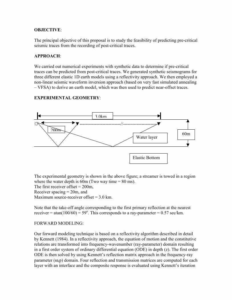
OBJECTIVE: The principal objective of this proposal is to study the feasibility of predicting pre-critical seismic traces from the recording of post-critical traces. APPROACH: We carried out numerical experiments with synthetic data to determine if pre-critical traces can be predicted from post-critical traces. We generated synthetic seismograms for three different elastic 1D earth models using a reflectivity approach. We then employed a non-linear seismic waveform inversion approach (based on very fast simulated annealing – VFSA) to derive an earth model, which was then used to predict near-offset traces. EXPERIMENTAL GEOMETRY: ☼ ▼---------------------------//----------------------▼ The expwhere thThe firsReceiveMaximu Note thareceiver FORWA Our forwby Kennrelationsin a firstODE is parametlayer wi

200m

erimental geometry is she water depth is 60m (T

t receiver offset = 200m,r spacing = 20m, and m source-receiver offset

t the take-off angle corr = atan(100/60) = 59o. T

RD MODELING:

ard modeling techniqueett (1984). In a reflectiv are transformed into fre order system of ordinarthen solved by using Keer (ω,p) domain. Four reth an interface and the co

3.0km

own in the above figure; a streamer is towed in a region wo way time = 80 ms).

= 3.0 km.

esponding to the first primary reflection at the nearest his corresponds to a ray-parameter = 0.57 sec/km.

is based on a reflectivity algorithm described in detail ity approach, the equation of motion and the constitutive quency-wavenumber (ray-parameter) domain resulting y differential equation (ODE) in depth (z). The first order nnett’s reflection matrix approach in the frequency-ray flection and transmission matrices are computed for each mposite response is evaluated using Kennett’s iteration

60mWater layer

Elastic Bottom

equation. The final response in the offset-time domain is computed by plane wave transformation of the data in the frequency-wavenumber domain. Intermediate results in the delay time – ray-parameter (τ-p) domain can be obtained simply by inverse temporal Fourier transformation. SOURCE WAVELET: We used a Ricker wavelet with a peak frequency of 40 Hz in all our applications to generate synthetic pressure response for the experimental geometry shown in the figure. OPTIMIZATION/WAVEFORM INVERSION: The details of the seismic waveform inversion are described in chapter 6 of Sen and Stoffa (1995). In a seismic waveform inversion, synthetic seismograms for an assumed earth model are compared with the recorded seismograms. If the match is not adequate, the model is perturbed until the fit is acceptable. Optimization methods are employed to update the model and to find an optimal model. The salient features of our approach are as follows:

• We use plane wave transformed data since forward modeling in this domain is extremely efficient,

• We use a global optimization method called very fast simulated annealing (VFSA) for model update and to find an optimal model,

• We use a normalized cross-correlation function that is sensitive to both amplitude and phase, as the objective function, and

• We carry out our search in a user-supplied search window enabling us to speed up the computation and restrict our search to realistic values of earth model parameters.

NUMERICAL EXPERIMENTS MODEL I: Soft Bottom The elastic parameters for this model are as follows: Vp = 1.7 km/sec, Vs = 0.8 km/sec, and Density = 1.3 gm/cc. Synthetic (x,t) gathers in the offset range of 0.2-3.0 km are shown in Fig 1. Realistic anelastic attenuation values were used in generating the synthetic seismograms. The data contain primary sea-floor reflections and several of its multiples along with the head waves. For this model, the critical angle is 61.9o, which corresponds to a ray-parameter of 0.588 sec/km. Thus we notice that we have pre-critical primary reflection only in the range of 59 o to 61.9 o, i.e., a ray-parameter range of 0.57 sec/km to 0.588 sec/km. All

other primary reflection arrivals are post-critical arrivals. The (x,t) gathers shown in Fig 1 were used to generate (τ-p) gathers in the ray-parameter range of 0.57 to 0.66 sec/km using a true-amplitude frequency-domain plane-wave transformation code. The primaries and all the multiples are clearly visible (Fig 2a). The search window used in the VFSA inversion is given below: Vpmin Vpmax Vsmin Vsmax Rhomin Rhomax TWT_m

in TWT_max

Layer 1 1.5 1.5 0.0 0.0 1.0 1.0 0.72 0.88 Layer 2 1.3 2.2 0.6 1.4 1.0 1.8 - - TWT : Two-way-time The best-fit model obtained by VFSA (dashed line) is compared with the true model in Fig. 2(b). We then computed seismograms in the offset range of 20m to 200m using the true and the reconstructed models. The difference between the two sets of seismograms is negligible (Fig. 3 right panel). MODEL 2: Hard Bottom The elastic parameters for this model are as follows: Vp = 2.0 km/sec, Vs = 0.8 km/sec, and Density = 1.4 gm/cc. Synthetic (x,t) gathers in the offset range of 0.2-3.0km are shown in Fig 4. The data contain primary sea-floor reflections and several of its multiples along with the head waves. For this model, the critical angle is 48.6o, which corresponds to a ray-parameter of 0.5 sec/km. Thus we record only the post-critical reflections the ray-parameter range of 0.57 sec/km to 0.588 sec/km. The (x,t) gathers shown in Fig 4 were used to generate (τ-p) gathers in the ray-parameter range of 0.57 to 0.66 sec/km using a true-amplitude frequency-domain plane-wave transformation code. The primaries and all the multiples are clearly visible (Fig 5a). The search window used in the VFSA inversion is given below: Vpmin Vpmax Vsmin Vsmax Rhomin Rhomax Twt_mi

n Twt_max

Layer 1 1.5 1.5 0.0 0.0 1.0 1.0 0.72 0.88 Layer 2 1.3 2.5 0.6 1.4 1.0 1.8 - - The best-fit model obtained by VFSA (dashed line) is compared with the true model in Fig. 5(b).

We then computed seismograms in the offset range of 20m to 200m using the true and the reconstructed models. The difference between the two sets of seismograms is small (Fig. 6 right panel). Next we added a small amount of (1%) random noise to the data shown in Fig 4 (Figure 7) and obtained (τ-p) gathers shown in Fig 8(a). The noisy (τ-p) data were then used in the waveform inversion; all other parameters were the same as those in the noise-free case. The results are shown in Figure 8(b) and the data predictions are shown in Fig. 9. MODEL 3: Multi-layered Case The elastic parameters of the model are given below: Layer No. Vp Vs Rho TWT 1 1.5 0.0 1.0 0.08 2 1.7 0.7 1.3 0.18 3 1.85 0.9 1.4 0.28 4 1.95 1.1 1.5 0.38 5 2.10 1.3 1.7 - Synthetic (x,t) gathers in the offset range of 0.2-3.0 km are shown in Fig 10. The data contain primary sea-floor and subsurface reflections and several of their multiples along with the head waves. For this model, the critical angle for the sea-floor primary is 61.9o, which corresponds to a ray-parameter of 0.588 sec/km. Thus we record sea-floor pre-critical reflections in the ray-parameter range of 0.57 sec/km to 0.588 sec/km. The (x,t) gathers shown in Fig 10 were used to generate (τ-p) gathers in the ray-parameter range of 0.49 to 0.66 sec/km using a true-amplitude frequency-domain plane-wave transformation code. The primaries and all the multiples are clearly visible (Fig 11a). Note that the sea-floor primaries in the range of 0.49-0.57 sec/km are not recorded in the offset range for this experiment. In the (τ-p) data, the sea-floor primaries in this range are transform artifacts (leakage) that can be considered noise. The search window used in the VFSA inversion is given below: Vpmin Vpmax Vsmin Vsmax Rhomin Rhomax Twt_mi

n Twt_max

Layer 1 1.5 1.5 0.0 0.0 1.0 1.0 0.72 0.88 Layer 2 1.3 1.9 0.5 0.9 1.0 1.5 0.16 0.20 Layer 3 1.5 2.0 0.7 1.1 1.2 1.6 0.26 0.30 Layer 4 1.8 2.2 0.9 1.3 1.3 1.7 0.36 0.40

Layer 5 1.8 2.3 1.1 1.5 1.5 1.9 - - The best-fit model obtained by VFSA (dashed line) is compared with the true model in Fig. 11(b). We then computed seismograms in the offset range of 20m to 200m using the true and the reconstructed models. The difference between the two sets of seismograms is negligible (Fig. 12 right panel). SUMMARY We generated reflectivity synthetic seismograms in the offset range 0.2-3.0 km for a shallow water experiment for a series of subsurface models. These were then used in a nonlinear VFSA inversion to predict earth models, which were then used to generate seismograms in the near-offset regions. Our experiments showed that in all of our experiments, we were able to predict the near-offset data reasonably well. Note that given the post-critical data alone, the inverse problem has non-unique solutions. In all cases, we made several inversion runs with different random starting models (within the search window) and obtained multiple solutions that are slightly different but have the same level of data misfit. In this report, we only showed one of the many models. Even with the broad search window used in all the inversion runs, we were able to obtain models that range within small values of the model parameters. In all cases the data prediction appears acceptable. Whether such data prediction is adequate for multiple attenuation can only be assessed with further studies using field data. Here we outline the following limitations of our approach. We assumed that

• The source-time function or the wavelet and the source and receiver depths are known exactly,

• In the multi-layered inversion (Model 3) we assumed prior knowledge of the number of subsurface reflectors,

• Direct waves were not included in the modeling and inversion (Arthur Weglein and one of his students are developing a robust algorithm for direct wave removal which can used in pre-processing of field data),

• The subsurface attenuation structure was assumed known. These limitations and deviation from 1D earth structure can cause potential errors in the real data inversion. Such problems should be addressed in a future study (possible second phase of the project) with application to real data. Nonetheless the results from using a very small range of ray-parameter are highly encouraging..

REFERENCE: Kennett, B. L. N., 1984, Seismic wave propagation in stratified media, The Cambridge

University Press. Sen, M. K., and P. L. Stoffa, 1995, Global optimization methods in geophysical

inversion, Elsevier Science Publishing Company, The Netherlands.

SOFT BOTTOM

0.000

0.312

0.625

0.938

1.250

1.562

1.875

2.188

2.500

2.812

3.125

3.438

3.750

4.062

4.375

4.688

5.0001

0.20 0.40 0.60 0.80 1.00 1.20 1.40 1.60 1.80 2.00 2.20 2.40 2.60 2.80 3.00

0.00

0.50

1.00

1.50

2.00

2.50

Shot Gather - Model Soft Bottom

Figure 1. Synthetic seismograms for a water layer over half-space (soft) model computed by using a full waveform modeling algorithm: Water layer reverberations and head waves are clearly visible.

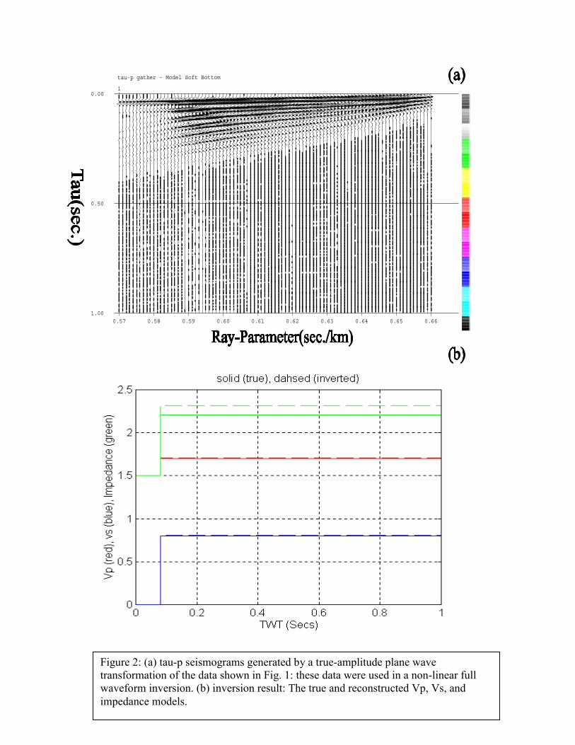
0.000

0.312

0.625

0.938

1.250

1.562

1.875

2.188

2.500

2.812

3.125

3.438

3.750

4.062

4.375

4.688

5.0001

0.57 0.58 0.59 0.60 0.61 0.62 0.63 0.64 0.65 0.66

0.00

0.50

1.00

tau-p gather - Model Soft Bottom

Figure 2: (a) tau-p seismograms generated by a true-amplitude plane wave transformation of the data shown in Fig. 1: these data were used in a non-linear full waveform inversion. (b) inversion result: The true and reconstructed Vp, Vs, and impedance models.

0.750

0.875

1.000

1.125

1.250

1.375

1.500

1.625

1.750

1.875

2.0001

0.02

0.00

0.50

1.00

Prediction of near traces

Predicted Data e

Figure 3: Data panel) are combetween the tw

True Data

0.12 0.02 0.12 0.02

Prediction: The near traces predicted by the reconstructed mpared with those for the true model (left panel). The differeno sets is very small.

Differenc

0.000

0.125

0.250

0.375

0.500

0.625

0.12

odel (middle ce (right panel)

HARD BOTTOM – NOISE FREE CASE

0.000

0.312

0.625

0.938

1.250

1.562

1.875

2.188

2.500

2.812

3.125

3.438

3.750

4.062

4.375

4.688

5.0001

0.20 0.40 0.60 0.80 1.00 1.20 1.40 1.60 1.80 2.00 2.20 2.40 2.60 2.80 3.00

0.00

0.20

0.40

0.60

0.80

1.00

1.20

1.40

1.60

1.80

2.00

2.20

2.40

2.60

2.80

x-t data (observation)
Figure 4. Synthetic seismograms for a water layer over half-space (hard bottom) model computed by
using a full waveform modeling algorithm: Water layer reverberations and head waves are clearly visible. Notice that in the offset range (0.2-3.0 km), only the post-critical arrivals are recorded.

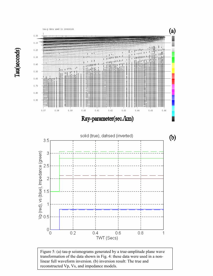
0.000

0.312

0.625

0.938

1.250

1.562

1.875

2.188

2.500

2.812

3.125

3.438

3.750

4.062

4.375

4.688

5.0001

0.57 0.58 0.59 0.60 0.61 0.62 0.63 0.64 0.65 0.66

0.00

0.10

0.20

0.30

0.40

0.50

0.60

0.70

0.80

0.90

tau-p data used in inversion


1.250

1.375

1.500

1.625

1.750

1.875

2.0001

0.01

0.00

0.50

1.00

seismic section display

Predicted Data e
True Data
0.11 0.210.01 0.11 0.210.01

Differenc

0.000

0.125

0.250

0.375

0.500

0.625

0.750

0.875

1.000

1.125

0.11 0.21

Figure 6: Data Prediction: The near traces predicted by the reconstructed model (middle panel) are compared with those for the true model (left panel). The difference (right panel) between the two sets is small.

Hard Bottom with Noise

0.000

0.312

0.625

0.938

1.250

1.562

1.875

2.188

2.500

2.812

3.125

3.438

3.750

4.062

4.375

4.688

5.0001

0.20 0.40 0.60 0.80 1.00 1.20 1.40 1.60 1.80 2.00 2.20 2.40 2.60 2.80 3.00

0.00

0.20

0.40

0.60

0.80

1.00

1.20

1.40

1.60

1.80

2.00

2.20

2.40

2.60

2.80

Noisy x-t data

`````

Figure 7. Synthetic seismograms for a water layer over half-space (hard bottom) model computed by using a full waveform modeling algorithm: Water layer reverberations and head waves are clearly visible. Notice that in the offset range (0.2-3.0 km), only the post-critical arrivals are recorded. These data are the same as those shown in fig. 4 with random noise added to them.

0.000

0.312

0.625

0.938

1.250

1.562

1.875

2.188

2.500

2.812

3.125

3.438

3.750

4.062

4.375

4.688

5.0001

0.57 0.58 0.59 0.60 0.61 0.62 0.63 0.64 0.65 0.66

0.00

0.10

0.20

0.30

0.40

0.50

0.60

0.70

0.80

0.90

1.00

1.10

1.20

1.30

1.40

1.50

1.60

1.70

1.80

1.90

Figure 8: (a) tau-p seismograms generated by a true-amplitude plane wave transformation of the data shown in Fig. 7: these data were used in a non-linear fullwaveform inversion. (b) inversion result: The true and reconstructed Vp, Vs, and impedance models.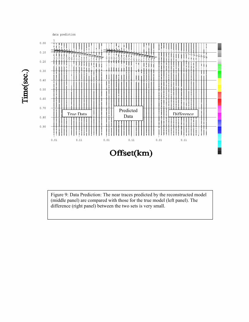

0.750

0.875

1.000

1.125

1.250

1.375

1.500

1.625

1.750

1.875

2.0001

0.01

0.00

0.10

0.20

0.30

0.40

0.50

0.60

0.70

0.80

0.90

data prediction

ePredicted

Data

Figure 9(middledifferen

True Data

0.11 0.01 0.11 0.01

: Data Prediction: The near traces predicted by the re panel) are compared with those for the true model (lece (right panel) between the two sets is very small.

Differenc

0.000

0.125

0.250

0.375

0.500

0.625

0.11

constructed model ft panel). The

Multi_layer Case

0.000

0.312

0.625

0.938

1.250

1.562

1.875

2.188

2.500

2.812

3.125

3.438

3.750

4.062

4.375

4.688

5.0001

0.20 0.40 0.60 0.80 1.00 1.20 1.40 1.60 1.80 2.00 2.20 2.40 2.60 2.80 3.00

0.00

0.20

0.40

0.60

0.80

1.00

1.20

1.40

1.60

1.80

2.00

2.20

2.40

2.60

2.80

x-t data

Figure 10. Synthetic seismograms for a water layer over multi-layered half-space (soft bottom) model computed by using a full waveform modeling algorithm: Water layer reverberations and head waves are clearly visible..

0.000

0.125

0.250

0.375

0.500

0.625

0.750

0.875

1.000

1.125

1.250

1.375

1.500

1.625

1.750

1.875

2.0001

0.49 0.50 0.51 0.52 0.53 0.54 0.55 0.56 0.57 0.58 0.59 0.60 0.61 0.62 0.63 0.64 0.65

0.00

0.50

1.00



0.625

0.750

0.875

1.000

1.125

1.250

1.375

1.500

1.625

1.750

1.875

2.0001

0.01

0.00

0.10

0.20

0.30

0.40

0.50

0.60

0.70

0.80

0.90

data prediction

Predicted Data e

True Data

0.11 0.01 0.11 0.01

Differenc

0.000

0.125

0.250

0.375

0.500

0.11

Figure 12: Data Prediction: The near traces predicted by the reconstructed model (middle panel) are compared with those for the true model (left panel). The difference (right panel) between the two sets is very small.

Documents

Copyright © 2006 M-OSRP Inc. All rights reserved. Report 2001-2002.pdf · Petrobras Jurandyr Schmidt Phillips Doug Foster Saudi Aramco Panos Kelamis Shell Jon Sheiman (Chairman)