Embed Size (px)
Citation preview

Copyright © 2005 Brooks/Cole, a division of Thomson Learning, Inc.1
Chapter 4
Numerical Methods for Describing Data

Copyright © 2005 Brooks/Cole, a division of Thomson Learning, Inc.2
Describing the Center of a Data Set with the arithmetic mean
1 2 n
sum of all observations in the samplex
number of observations in the sample
x x x x
n n
The sample mean of a numerical sample, x1, x2, x3,…, xn, denoted
, is
The sample mean of a numerical sample, x1, x2, x3,…, xn, denoted
, is

Copyright © 2005 Brooks/Cole, a division of Thomson Learning, Inc.3
Describing the Center of a Data Set with the arithmetic mean
The population mean is denoted by µ, is the average of all x values in the entire population.

Copyright © 2005 Brooks/Cole, a division of Thomson Learning, Inc.4
The “average” or mean price for this sample of 10 houses in Fancytown is $295,000
Example calculations
During a two week period 10 houses were sold in Fancytown.
x 2,950,000x
n 10295,000
House Price in Fancytown
x231,000313,000299,000312,000285,000317,000294,000297,000315,000287,000
2,950,000x

Copyright © 2005 Brooks/Cole, a division of Thomson Learning, Inc.5
Describing the Center of a Data Set with the median
The sample median is obtained by first ordering the n observations from smallest to largest (with any repeated values included, so that every sample observation appears in the ordered list). Then
the single middle value if n is oddsample median=
the mean of the middle two values if n is even
Copyright © 2005 Brooks/Cole, a division of Thomson Learning, Inc.6
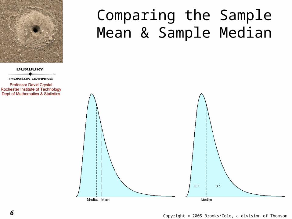
Comparing the Sample Mean & Sample Median

Copyright © 2005 Brooks/Cole, a division of Thomson Learning, Inc.7
Comparing the Sample Mean & Sample Median

Copyright © 2005 Brooks/Cole, a division of Thomson Learning, Inc.8
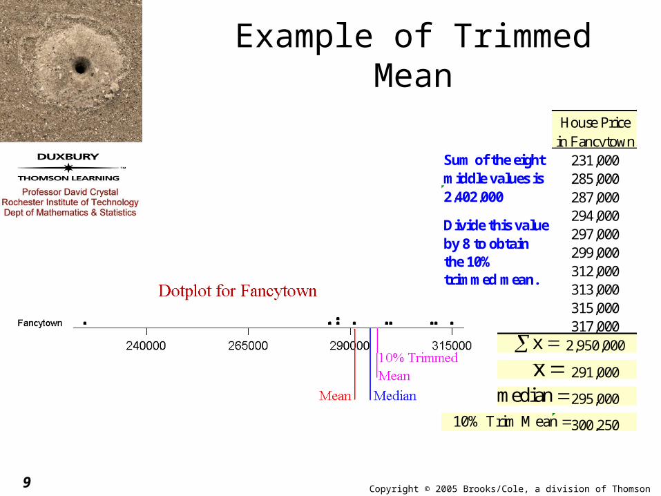
The Trimmed Mean
A trimmed mean is computed by first ordering the data values from smallest to largest, deleting a selected number of values from each end of the ordered list, and finally computing the mean of the remaining values.
The trimming percentage is the percentage of values deleted from each end of the ordered list.
Copyright © 2005 Brooks/Cole, a division of Thomson Learning, Inc.9
Example of Trimmed Mean
House Price in Fancytown
231,000285,000287,000294,000297,000299,000312,000313,000315,000317,000
2,950,000
291,000
295,000
300,250
2,402,000
Sum of the eight middle values is
Divide this value by 8 to obtain the 10% trimmed mean.
x x
median 10% Trim Mean

Copyright © 2005 Brooks/Cole, a division of Thomson Learning, Inc.10
Categorical Data - Sample Proportion
The sample proportion of successes, denoted by p, is
Where S is the label used for the response designated as success.The population proportion of successes is denoted by .
p sample proportion of successesnumber of S's in the sample
n
The sample proportion of successes, denoted by p, is
Where S is the label used for the response designated as success.The population proportion of successes is denoted by .
p sample proportion of successesnumber of S's in the sample
n

Copyright © 2005 Brooks/Cole, a division of Thomson Learning, Inc.11
If we look at the student data sample, consider the variable gender and treat being female as a success, we have 25 of the sample of 79 students are female, so the sample proportion (of females) is
Categorical Data - Sample Proportion
25p 0.31679

Copyright © 2005 Brooks/Cole, a division of Thomson Learning, Inc.12
Describing Variability
The simplest numerical measure of the variability of a numerical data set is the range, which is defined to be the difference between the largest and smallest data values.
range = maximum - minimum

Copyright © 2005 Brooks/Cole, a division of Thomson Learning, Inc.13
Describing Variability
The n deviations from the sample mean are the differences:
Note: The sum of all of the deviations from the sample mean will be equal to 0, except possibly for the effects of rounding the numbers. This means that the average deviation from the mean is always 0 and cannot be used as a measure of variability.
1 2 2 nx x, x x, x x, , x x,

Copyright © 2005 Brooks/Cole, a division of Thomson Learning, Inc.14
Sample Variance
The sample variance, denoted s2 is the sum of the squared deviations from the mean divided by n-1.
22 xx
(x x) Ss
n 1 n 1
2 2 2xx 1 2 n
2
S (x x) (x x) (x x)
x x
Note:
2 2 2xx 1 2 n
2
S (x x) (x x) (x x)
x x
Note:

Copyright © 2005 Brooks/Cole, a division of Thomson Learning, Inc.15
Sample Standard Deviation
The sample standard deviation, denoted s is the positive square root of the sample variance.
The population standard deviation is denoted by .
22 xx
(x x) Ss s
n 1 n 1

Copyright © 2005 Brooks/Cole, a division of Thomson Learning, Inc.16
Example calculations
10 Macintosh Apples were randomly selected and weighed (in ounces).
Range 8.48 6.24 2.24
x 74.24x 7.424
n 10
22 (x x) 5.5398
sn 1 10 1
5.53980.61554
9
s= 0.61554 0.78456
x7.52 0.096 0.00928.48 1.056 1.11517.36 -0.064 0.00416.24 -1.184 1.40197.68 0.256 0.06556.56 -0.864 0.74656.40 -1.024 1.04868.16 0.736 0.54177.68 0.256 0.06558.16 0.736 0.541774.24 0.000 5.5398
x x 2(x x)

Copyright © 2005 Brooks/Cole, a division of Thomson Learning, Inc.17
Calculator Formula for s2 and s
A computational formula for the sample variance is given by
A little algebra can establish the sum of the square deviations,
2
2 2xx
xS (x x) x n
2
2
2 xx
xxS ns
n 1 n 1

Copyright © 2005 Brooks/Cole, a division of Thomson Learning, Inc.18
Calculations Revisited
The values for s2 and s are exactly the same as were obtained earlier.
x x2
7.52 56.55048.48 71.91047.36 54.16966.24 38.93767.68 58.98246.56 43.03366.40 40.96008.16 66.58567.68 58.98248.16 66.585674.24 556.6976
2n 10, x 74.24, x 556.6976
2
2xx
2
xS x n
(74.24)556.6976 5.53984
10
2 5.53984s 0.615538
9
s 0.615538 0.78456

Copyright © 2005 Brooks/Cole, a division of Thomson Learning, Inc.19
Quartiles and the Interquartile Range
Lower quartile (Q1) = median of the lower half
of the data set.
Upper Quartile (Q3) = median of the upper half of the data set.
Note: If n is odd, the median is excluded from both the lower and upper halves of the data.
The interquartile range (iqr), a resistant measure of variability is given by
iqr = upper quartile – lower quartile
= Q3 – Q1

Copyright © 2005 Brooks/Cole, a division of Thomson Learning, Inc.20
Skeletal Boxplot Example
Using the student work hours data we have
0 5 10 15 20 25

Copyright © 2005 Brooks/Cole, a division of Thomson Learning, Inc.21
Outliers
An observations is an outlier if it is more than 1.5 iqr away from the closest end of the box (less than the lower quartile minus 1.5 iqr or more than the upper quartile plus 1.5 iqr.
An outlier is extreme if it is more than 3 iqr from the closest end of the box, and it is mild otherwise.

Copyright © 2005 Brooks/Cole, a division of Thomson Learning, Inc.22
Modified Boxplots
A modified boxplot represents mild outliers by shaded circles and extreme outliers by open circles. Whiskers extend on each end to the most extreme observations that are not outliers.

Copyright © 2005 Brooks/Cole, a division of Thomson Learning, Inc.23
Modified Boxplot Example
Using the student work hours data we have
0 5 10 15 20 25
Lower quartile + 1.5 iqr = 14 - 1.5(6) = -1
Upper quartile + 1.5 iqr = 14 + 1.5(6) = 23
Smallest data value that isn’t
an outlier
Largest data value that isn’t
an outlier
Upper quartile + 3 iqr = 14 + 3(6) = 32
MildOutlier

Copyright © 2005 Brooks/Cole, a division of Thomson Learning, Inc.24
Modified Boxplot ExampleConsider the ages of the 79 students from the classroom data set from the slideshow Chapter 3.
Iqr = 22 – 19 = 3
17 18 18 18 18 18 19 19 19 19 19 19 19 19 19 19 19 19 19 19 19 19 19 19 19 19 20 20 20 20 20 20 20 20 20 20 21 21 21 21 21 21 21 21 21 21 21 21 21 21 22 22 22 22 22 22 22 22 22 22 22 23 23 23 23 23 23 24 24 24 25 26 28 28 30 37 38 44 47
Median
Lower Quartile
Upper Quartile
Moderate Outliers Extreme Outliers
Lower quartile – 3 iqr = 10 Lower quartile – 1.5 iqr =14.5Upper quartile + 3 iqr = 31 Upper quartile + 1.5 iqr = 26.5

Copyright © 2005 Brooks/Cole, a division of Thomson Learning, Inc.25
Smallest data value that isn’t
an outlier
Largest data value that isn’t
an outlier
MildOutliers
ExtremeOutliers
15 20 25 30 35 40 45 50
Modified Boxplot Example
Here is the modified boxplot for the student age data.

Copyright © 2005 Brooks/Cole, a division of Thomson Learning, Inc.26
Modified Boxplot Example
50
45
40
35
30
25
20
15
Here is the same boxplot reproduced with a vertical orientation.

Copyright © 2005 Brooks/Cole, a division of Thomson Learning, Inc.27
Comparative Boxplot Example
100 120 140 160 180 200 220 240
Females
MalesGender
Student Weight
By putting boxplots of two separate groups or subgroups we can compare their distributional behaviors.Notice that the distributional pattern of female and male student weights have similar shapes, although the females are roughly 20 lbs lighter (as a group).

Copyright © 2005 Brooks/Cole, a division of Thomson Learning, Inc.28
Interpreting VariabilityChebyshev’s Rule
2
1100 1 %
k
Chebyshev’s Rule
Consider any number k, where
k 1. Then the percentage of observations that are within k standard deviations of the mean is at least .
2
1100 1 %
k
Chebyshev’s Rule
Consider any number k, where
k 1. Then the percentage of observations that are within k standard deviations of the mean is at least .

Copyright © 2005 Brooks/Cole, a division of Thomson Learning, Inc.29
For specific values of k Chebyshev’s Rule readsAt least 75% of the observations are within 2 standard
deviations of the mean. At least 89% of the observations are within 3 standard
deviations of the mean. At least 90% of the observations are within 3.16
standard deviations of the mean. At least 94% of the observations are within 4 standard
deviations of the mean. At least 96% of the observations are within 5 standard
deviations of the mean.
At least 99% of the observations are with 10 standard deviations of the mean.
Interpreting VariabilityChebyshev’s Rule

Copyright © 2005 Brooks/Cole, a division of Thomson Learning, Inc.30
Consider the student age data
Example - Chebyshev’s Rule
17 18 18 18 18 18 19 19 19 1919 19 19 19 19 19 19 19 19 1919 19 19 19 19 19 20 20 20 2020 20 20 20 20 20 21 21 21 2121 21 21 21 21 21 21 21 21 2122 22 22 22 22 22 22 22 22 2222 23 23 23 23 23 23 24 24 2425 26 28 28 30 37 38 44 47
Color code: within 1 standard deviation of the meanwithin 2 standard deviations of the meanwithin 3 standard deviations of the meanwithin 4 standard deviations of the meanwithin 5 standard deviations of the mean

Copyright © 2005 Brooks/Cole, a division of Thomson Learning, Inc.31
Summarizing the student age data
Example - Chebyshev’s Rule
Interval Chebyshev’s Actual
within 1 standard deviation of the mean
0% 72/79 = 91.1%
within 2 standard deviations of the mean
75% 75/79 = 94.9%
within 3 standard deviations of the mean
88.8% 76/79 = 96.2%
within 4 standard deviations of the mean
93.8% 77/79 = 97.5%
within 5 standard deviations of the mean
96.0% 79/79 = 100%
Notice that Chebyshev gives very conservative lower bounds and the values aren’t very close to the actual percentages.

Copyright © 2005 Brooks/Cole, a division of Thomson Learning, Inc.32
Empirical Rule
If the histogram of values in a data set is reasonably symmetric and unimodal (specifically, is reasonably approximated by a normal curve), then
1. Approximately 68% of the observations are within 1 standard deviation of the mean.
2. Approximately 95% of the observations are within 2 standard deviation of the mean.
3. Approximately 99.7% of the observations are within 3 standard deviation of the mean.

Copyright © 2005 Brooks/Cole, a division of Thomson Learning, Inc.33
Z Scores
The z score is how many standard deviations the observation is from the mean.
A positive z score indicates the observation is above the mean and a negative z score indicates the observation is below the mean.
The z score corresponding to a particular observation in a data set is
observation meanzscorestandard deviation
The z score corresponding to a particular observation in a data set is
observation meanzscorestandard deviation

Copyright © 2005 Brooks/Cole, a division of Thomson Learning, Inc.34
Computing the z score is often referred to as standardization and the z score is called a standardized score.
Z Scores
x xz score s
The formula used with sample data is
x xz score s
The formula used with sample data is

Copyright © 2005 Brooks/Cole, a division of Thomson Learning, Inc.35
Example
A sample of GPAs of 38 statistics students appear below (sorted in increasing order)2.00 2.25 2.36 2.37 2.50 2.50 2.602.67 2.70 2.70 2.75 2.78 2.80 2.802.82 2.90 2.90 3.00 3.02 3.07 3.153.20 3.20 3.20 3.23 3.29 3.30 3.30 3.42 3.46 3.48 3.50 3.50 3.58 3.75 3.80 3.83 3.97
x 3.0434 and s 0.4720

Copyright © 2005 Brooks/Cole, a division of Thomson Learning, Inc.36
ExampleThe following stem and leaf indicates that the GPA data is reasonably symmetric and unimodal.
2 02 2332 552 6677772 888993 00013 22222333 4445553 73 889
Stem: Units digitLeaf: Tenths digit

Copyright © 2005 Brooks/Cole, a division of Thomson Learning, Inc.37
Example
Using the formula we compute the z scores and color code the values as we did in an earlier example.
-2.21 -1.68 -1.45 -1.43 -1.15 -1.15-0.94 -0.79 -0.73 -0.73 -0.62 -0.56-0.52 -0.52 -0.47 -0.30 -0.30 -0.09-0.05 0.06 0.23 0.33 0.33 0.330.40 0.52 0.54 0.54 0.80 0.880.93 0.97 0.97 1.14 1.50 1.601.67 1.96
x xz score sUsing the formula we compute
the z scores and color code the values as we did in an earlier example.
-2.21 -1.68 -1.45 -1.43 -1.15 -1.15-0.94 -0.79 -0.73 -0.73 -0.62 -0.56-0.52 -0.52 -0.47 -0.30 -0.30 -0.09-0.05 0.06 0.23 0.33 0.33 0.330.40 0.52 0.54 0.54 0.80 0.880.93 0.97 0.97 1.14 1.50 1.601.67 1.96
x xz score s

Copyright © 2005 Brooks/Cole, a division of Thomson Learning, Inc.38
Example
Interval Empirical Rule Actual
within 1 standard deviation of the mean
68% 27/38 = 71%
within 2 standard deviations of the mean
95% 37/38 = 97%
within 3 standard deviations of the mean
99.7% 38/38 = 100%
Notice that the empirical rule gives reasonably good estimates for this example.