COPY: KIRTLAND

-

NASA TECHNICAL NOTE 1 N A S A TN D-5434

LOAN COPY: RETURh i LJ

AFWL (WuDL-2j KIRTLAND AFB, N ME':

A MODIFIED METHOD OF INTEGRAL RELATIONS APPROACH TO THE BLUNT-BODY EQUILIBRIUM AIR FLOW FIELD, INCLUDING COMPARISONS WITH INVERSE SOLUTIONS

b,y L. Bertzurd Garrett and John T. Suttles Langley Research Center and Joh~z N. Perkim North Carolinu State University

N A T I O N A L A E R O N A U T I C S A N D S P A C E A D M I N I S T R A T I O N W A S H I N G T O N , D. C. S E P T E M B E R 1 9 6 9

TECH LIBRARY KAFB, NM

1. Report No.

NASA TN 0-5434 I 2. Government Accession No.

4. T i t l e a n d S u b t i t l e A MODIFIED METHOD OF INTEGRAL RELATIONS APPROACH TO THE BLUNT- BODY EQUILIBRIUM AIR FLOW FIELD, INCLUDING COMPARISONS WITH INVERSE SOLUTIONS

7. Author(s)

L. Bernard Garret t , John T. Suttles, a n d J o h n N. Pe rk ins (John N. Perk ins f rom Nor th Caro l ina S ta te Un ivers i ty )

9. Performing Orgonizat ion Name and Address

NASA Langley Research Center

Hampton, Va. 23365

2. Sponsoring Agency Nome and Address

National Aeronautics and Space Administrat ion

Washington, D.C. 20546

3. Recipient ’s Cotolog N

5. Report Dote September 1969

6. Performing Orgonizot i

8. Performing Orgonizot i L- 6209

10. Work U n i t N o .

124-07-18-01-23 1 1 . Controct or Gront No.

13. T y p e o f Report ond P

Technical Note

14. sponsoring Agency C(

5. Supplementary Notes

APPENDIX C: A CORRELATION OF EQUILIBRIUM AIR PROPERTIES TO 150000 K

By G. Louis Smi th and L. Bernard Garret t

6 . Abstract

A modified approach to the f i rst-order approximat ion of the method of integral relat ions is prese

for the numer ica l ca lcu lat ion of the inviscid, adiabatic f low f ield around a blunt-nose body travel ing i

hypersonic speeds. Solutions have been obtained and computed f low-field data are presented for the

adiabatic steady flow of a perfect gas a n d a i r in chemical equi l ibr ium. The results obtained by the pr

method of solution are compared with results obtained by us ing inverse methods, property-derivative i

gral relat ions methods, and experiment. The results indicate that the present method provides an acc

versati le solut ion of the blunt-body f low f ield, and the relat ive simplici ty of the method should a l low I

sion to coupled radiating flow-field analyses.

17. K e y Words Suggested by Author(s) Blunt-body f low fields

Integral re lat ions solut ions

__

118. Distribution Stotement

Unclassified - Unl imited

IO.

on Code

on Report No.

er iod Covered

>de

Direct method

Equ i l ib r ium a i r cor re la t ion

19. Securi ty Clossif . (of this report) 2; 21. No. o f P a g e s 20. Securi ty Clossif . (of this poge)

Unclassified 92 Unclassified

“For sale by the Clear inghouse for Federal Scient i f ic and Technical Informat ion Springfield, Virginia 22151

~~

A MODIFIED METHOD O F INTEGRAL RELATIONS APPROACH TO THE

BLUNT-BODY EQUILIBRIUM AIR. FLOW FIELD, INCLUDING

COMPARISONS WITH INVERSE SOLUTIONS

By L. Bernard Garrett, John T. Suttles Langley Research Center

and

John N. Perkins North Carolina State University

SUMMARY

A modified approach to the first-order approximation of the method of integral relations is presented for the numerical calculation of the inviscid, adiabatic flow field around a blunt-nose body traveling at hypersonic speeds. Solutions have been obtained and computed flow-field data are presented for the adiabatic steady flow of a perfect gas and air in chemical equilibrium. The results obtained by the present method of solution are compared with results obtained by using inverse methods, property-derivative integral relations methods, and experiment. The results indicate that the present method provides an accurate, versatile solution of the blunt-body flow field, and the relative simplicity of the method should allow extension to coupled radiating flow-field analyses.

INTRODUCTION

Design for interplanetary spacecraft depends on a realistic definition of the entire flow field surrounding the body. The flow-field solutions should provide the necessary inputs required for the calculation of aerodynamic loads, shear stresses, radio attenua- tion regions, and convective and radiative heating. At hyperbolic speeds a predominant consideration is the radiation fluxes which are strongly dependent upon the distribution of the fluid properties and the chemical species between the shock and the body. At these velocities the energy losses due to radiation can have a significant effect on the entire flow field.

The purpose of this report is to develop an approximate numerical method which has promise for application in coupled radiating flow-field analyses and to compare

adiabatic-shock-layer results with other existing numerical solutions and with experimental data.

A method of integral-relations approach, which was first applied by Belotserkovskii (ref. 1) and Traugott (ref. 2) to the flow of a perfect gas over a blunt body, is employed in this analysis. A one-strip approximation is used. The solution is obtained by integrating a se t of governing differential equations which are cast in t e rms of the "fluxes" (mass, momentum, etc.) or "complexes" which was originally recommended by Lun'kin et al. (ref. 3) and Kao (ref. 4) and is employed extensively by Belotserkovskii (ref. 5) near the sonic region of the flow field. This approach is in contrast to prior approaches (see ref. 6, for example) in which the governing equations are written in terms of deriva- t ives of properties (velocity, pressure, etc.). The flow equations are developed without imposing the constancy of the entropy along streamlines; thus, the method can be extended to coupled radiation flow-field analyses. The approach is made more flexible in that the thermodynamic characterization of the fluid does not enter directly into the governing differential equations, but enters the governing system of equations only through auxiliary equations of state.

Flow-field results are presented for the adiabatic steady flow of a perfect gas and air in chemical equilibrium. The primary goal of this research is to examine the equilibrium air results obtained from the relatively simple one-strip integral approach to determine whether the solution is sufficiently accurate for use in adiabatic radiation computations such as were done by Kuby, et al. (ref. 7) .

The perfect gas model is employed primarily to study the basic flow-field approach, namely, to determine whether the formulation of the problem using the "flux" o r "com- plex" method has any computational advantages in the sonic region over the property- derivative method. The perfect gas model also permits a direct comparison of the flow-field results with other numerical procedures which use the same model: hence, differences in the results cannot be attributed to differences in real gas models.

SYMBOLS

4 coefficients in governing differential equations, defined in appendix A

Bj coefficients in governing differential equations, defined in appendix A

7'0 defined by equations (22)

C coefficient in governing differential equations, defined in appendix A

2

Ej coefficients in governing differential equations, defined in appendix A

Gj functions appearing in governing partial differential equations which are differentiated with respect to y (see eq. (5))

h static enthalpy

* h specific enthalpy divided by gas constant for cold air, OK (see appendix C )

H total enthalpy, u2 + v2 2

1 j functions appearing in governing partial differential equations which are differentiated with respect to x, defined by equations (9)

Kj nonhomogeneous functions in transformed governing partial differential equations, defined by equations (9)

j ,k,N integers

M Mach number

1

Pj = 6 P j

P

PEef

Q

qR

qRx 7qRy

R

r

pressure

reference pressure used for appendix C , 1.01325 X lo6 dynes/cm2

curvature of reference surface, 1 ii;;

radiation flux vector

radiation flux components in x and y directions, respectively

nondimensional gas constant, R’ Tb, WUL2

radius measured from axis of symmetry of body (see fig. 1)

3

11111 I"

R' universal gas constant

R;ef gas constant used in appendix C and based on pkef, pEef, and Wref,

Rb

RF

R;s

T'

VR

- W

X

Y

Z

z

P

Y

6

60

body radius of curvature (see fig. 1)

radiation flux term, defined in appendix A

body radius of curvature at x = 0

temperature, OK

free-stream velocity

velocity components in the x and y directions, respectively

resultant velocity

mean molecular weight of equilibrium air, g/g-mole (see appendix C)

mean molecular weight of cold air, 28.96 g/g-mole (see appendix C)

coordinate along body surface (see fig. 1)

coordinate normal to body surface (see fig. 1) -

compressibility, W r e f W

axial coordinate (see fig. 1)

constant

ratio of specific heats

shock displacement distance (see fig. 1)

shock displacement distance at axis of symmetry (x = 0)

4

60* converged value of shock displacement distance at axis of symmetry

r expression defined in appendix C (eq. (C8))

rl transformed y-coordinate, 8 Y

eb body inclination angle (see fig. 1)

K metric coefficient, 1 c Q6q

V expression defined in appendix C (eq. (C16))

5 expression defined in appendix C (eq. (C18))

P density

PE ef reference density used in appendix C, 1.29313 X g/cm3

expression defined in appendix C (eq. (C12))

w shock-wave angle (see fig. 1)

Subscripts:

b re fers to body

j re fers to a particular governing differential equation: 1 shock geometry equation 2 continuity equation 3 x-momentum equation 4 y-momentum equation 5 energy equation

shock-oriented properties (see sketch (a), appendix D)

r e fe r s t o conditions at axis of symmetry on the body

refers to conditions at body surface, q = 0

5

1 refers t o conditions immediately behind shock wave, r] = 1

stag refers to stagnation-point conditions

r ] variation with 7

00 dimensional free-stream conditions

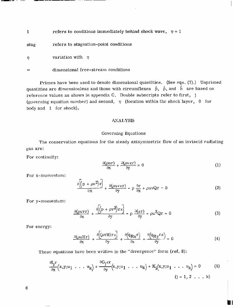
P r imes have been used to denote dimensional quantities. (See eqs. (7).) Unprimed quantities are dimensionless and those with circumflexes 6 , c , and fi are based on reference values as shown in appendix C. Double subscripts refer to first, j (governing equation number) and second, 7 (location within the shock layer, 0 for body and 1 for shock).

ANALYSIS

Governing Equations

The conservation equations for the steady axisymmetric flow of an inviscid radiating gas are:

For continuity:

For x-momentum:

For y-momentum:

For energy:

These equations have been written in the "divergence" form (ref. 8):

( j = 1 , 2 . . . k)

6

c I

where x,y are the independent variables, u1 . . Uk are the unknown functions, and I-,G.,K- are the known functions of x,y;ul . . . Uk. 3 3 3

The relationship between the shock and the body geometry in the body-oriented orthogonal coordinate system shown in figure 1 is

The quantities have been nondimensionalized as follows (primes denote dimensional quantities):

y = - Y' R.;j

Q = Q'RL 1 H = - PI'

(UL,)

It is desirable to transform the independent variables x,y to the normalized variables x , ~ where q = y/6 and 6 = 6fx). When the transformation is made, equation (5) becomes

where . 6

I1 = i; GI = 0 IC1 = --(I + Q6)tan w - I2 = pu G2 = pv K2 = 0

(

14 = ~ U V G4 = p + pv K4 = -(Qr + K COS eb)P - Qrpu2

I5 = puH Gg = pvH K g = - - : :qPrqR)

7

The relation Kg has been established by making the local-tangent slab approximation where flow properties for the radiation computations are assumed to be constant in planes tangent to the body and therefore

Application - of the ~~ method . of integral relations.- The method of integral relations reduces the system of nonlinear partial differential equations to an approximate set of nonlinear ordinary differential equations which can be integrated numerically.

.~ .

The basic approach is first to divide the region between the body and the shock into N s t r ips by using arbitrary values of 77 and then to represent certain combinations of the properties by interpolation polynomials in 77, the coefficients of which are evaluated at the strip boundaries. Finally, the system of equations is integrated from q = 0 to the boundary of each of the str ips to give N(j - 1) + 1 independent equaiions. (It is noted that the j = 1 equation relates the shock shape to the body geometry and thus is independent of the number of strips taken.)

The one-strip approximation is employed in this analysis. For simplicity, the functions Ij are assumed to vary l inearly in q ac ross the shock layers; that is,

Higher degree interpolation polynomials have been tried in the one-strip approach; they complicate the method without a noticeable improvement in the accuracy of the computations.

The governing equation (8) can now be integrated once over the shock layer from the body ( q = 0) to the shock ( q = 1) and then differentiated with respect to x to yield ordinary first-order differential equations of the form:

A detailed development of the governing equation (11) and the coefficients are given in appendix A.

Equations (6) and (11) constitute a system of five governing differential equations with the five unknown dependent variables 6, w , 120, ICJ~ , and 150. (Note thzt 140 = 0 for all x when the boundary conditions vo = 0 and dvo/dx = 0 are applied.) The derivatives which are specified by the governing differential equations are computed suc- cessively in the following order:

a

dx C

dx C

Note that the exact x-momentum equation (15) is used in lieu of the approximate relation. Experience has shown that numerical instabilities can be a serious problem in the €low-field calculations. For the one-strip approach with a linear approximation (the method being reported), this problem can be eliminated by replacing the approximate x-momentum equation at the body with the exact x-momentum equatior: Equation (15) can be used for nonequilibrium and radiating flow-field analyses where the flow along the body streamline is not isentropic.

Initial values.- In order to begin the integration of the governing differential equations (eqs. (12) to (16)), it is necessary to obtain initial values of the quantities appearing in the right-hand side of these equations. Direct substitution of the initial values at x = 0 results in indeterminate (O/O) expressions. Application of L'Hospital 's rule yields the proper starting values for the nonzero derivatives

dx

9

where RF is the radiation transport from the slab and is defined in appendix A (eq. (A12)). In the present analysis the radiation flux term RF is set equal to zero. (For a radiating shock layer, an iteration scheme can be used in which RF is initially assumed and compared with the computed radiation flux at the stagnation streamline.) Appendix B presents a detailed development of the initial value expressions.

The equations for the initial values (eqs. (17) to (19)) contain 6, the shock displacement distance at the axis of symmetry (x = 0). Since this term is an unknown in the problem, it is necessary to have a basis for establishing the correct 6, and hence a unique fiow-field solution. The logic for the uniqueness is based on the existence in the solution of the "sonic singular point." (See ref. 1.) The singular behavior in the solution provides a basis for i terating to establish the correct 6,. This aspect of the problem is discussed in detail in the section on the initial-value sensitivity study.

___ F h x and .. . properky evaluations.- The basic governing differential equations and the coefficients have been developed by considering only the fluid. mechanics of the flow field. In order to solve these equations, it is necessary to evaluate the thermodynamic properties properly. The present analysis is conducted for both perfect gases ( y = Constant) or equilibrium air. The thermodynamic properties for the equilibrium air model are correlated in appendix C from the equilibrium air data of Hilsenrath and Klein (ref. 9).

. . .

The conditions immediately behind the shock are computed from standard Rankine- Hugoniot relations for oblique shocks. The detailed shock equations used in this analysis are presented in appendix D for the perfect gas and equilibrium air models.

Perfect gas analysis: In the perfect gas analysis the stagnation properties on the body a r e computed exactly from the following relations:

In this modified method the properties on the body surface ( q = 0) a r e functions of the fluxes and are computed from the following simple algebraic equations:

10

212 0 uo =

-bo * (bo2 - 4c0

where

-2~130 b -

o - y(2R + 1) - 1

(Y + 1)1202 co =

y(2R + 1) - 1 I I2 0

P o = - UO

The sign outside the radical in the uo expression is positive in the subsonic region and negative in the supersonic region.

The linear variations between body and shock values fo r Ijv and also for p,u17 2 are employed. Thus, at ail other values of a r e computed from the following relations:

q across the shock-layer, the properties

Equilibrium air analysis: The thermodynamic properties for the equilibrium air model are correlated in appendix C from the Hilsenrath and Klein data for air in chemical equilibrium at temperatures up to 15 OOOo K. (See ref. 9.) The work in appendix C is presented in the form of a set of correlation formulas for the equilibrium thermodynamic properties of air. These formulas are used in the present method since their use resul ts in a considerable savings in computational time. The air correlation results are of the form:

11

P = P(P,h)

Z = Z(p,h)

where

u + v 2 2 2

h = H -

The temperature, in degrees Kelvin, is given by

In the perfect gas analysis the stagnation properties are computed exactly as functions of M, and y ; this computation is consistent with the formulation of the problem. However, in the equilibrium air analysis, which contains the pressure correlation, no convenient expressions exist for determining the exact stagnation properties. An approach is desired for computing the stagnation properties which is consistent with the approximations of the basic numerical approach, is extendable to the coupled radiating flow problem, and is not unduly complicated. Two approaches which meet these requirements are: (1) an assumption that the stagnation pressure is equal to the total pressure immediately behind the normal shock; that is,

1 2 " p + - p v Pstag 1 2 1 1

which is accurate to within 2 percent of the exact stagnation pressure for hypersonic f ree-s t ream Mach numbers; and (2) use of the limiting form of the x-momentum equation in the set of initial value equations (eqs. (17) to (19)), which gives

and an assumption of Newtonian form for (3)x=o, that is,

where p is a constant. For a spherical body, modified Newtonian theory indicates that p = -2.0 and modified theory with centrifugal correction indicates /3 = -2.67, whereas the pressure correlation of reference 10 gives p = -2.5. The numerical results obtained from these two assumptions are discussed in subsequent sections of this report.

12

A Newton-Raphson iteration technique is used to obtain the set of properties on the body which are consistent with the Ijs fluxes. The distributions of the properties across the shock layer are then computed from the following relations:

where the linear approximations for the Ijq (j = 2,4,5) terms are employed. (See

eq. (IO).) As a result of observing the near-linear resultant velocity distribution across the

shock layer, which was generated by the inverse solutions, the resultant velocity in the present equilibrium air analysis is assumed to vary linearly in q; that is,

VRq = vRO (vR1 - vRO)q (33)

The tangential velocity component and the static enthalpy expressions become

The pressure distribution is then computed from the quadratic expression

The coefficient of the f irst-order term in equation (36) is obtained from the exact y o r ' q momentum equation upon applying the boundary conditions at q = 0 that vo = 0 and Emo/& = 0. The remaining state properties are computed from the thermodynamic correlations:

(37)

Initial-Value Sensitivity Study

The blunt-body flow field is of the mixed flow type which requires the solution to elliptic equations in the subsonic region and hyperbolic equations in the supersonic region.

13

The supersonic solution introduces no special problems beyond hyperbolic stability con- siderations. However, singularities are present in the governing equations in the transonic region which require, for uniqueness, the solution of a. two-point boundary problem. (See ref. 1.) The subsonic solution, in the one-strip approximation, requires an initial value of the shock displacement distance 6, (at the axis of symmetry) which wil l satisfy a regularity condition at the natural sonic point on the body, the location of which is not known a priori .

In the property derivative formulation of the problem (refs. 1, 2 , 5, and S), the singularity in the transonic region is manifested in the equation for duo/& which has a denominator that vanishes when uo attains the sonic value. The basic procedure is to refine 6, until both the numerator and denominator of the equation for duo/& simultaneously approach zero within some predetermined accuracy constraint. The velocity derivative is then extrapolated into the supersonic region from a point where the velocity is within a certain percent of sonic velocity (around 95 percent)..

Xerikos and Anderson (ref. 6) conclude that 6, must be refined beyond eight significant figures in order to maintain downstream accuracy. Calculations (unpublished) have been made by J e r r y C. South, Jr., of the Langley &search Center by using a property-derivative integral method. South's analysis has shown for the sphere at M, = 5.017, y = 1.4, that for a perturbation in the fifth place in 6,, the tangential velocity derivative behaves erratica.!ly for a sxall distance downstream of the sonic point. However, the integral curve of uo was virtually unchanged from the solution generated with a 6, which w a s accurate to about eight significant figures.

In the flux formulation of the problem (refs. 3 , 4, 5, and l l ) , the boundary conditions, at the sonic point on the body, of finite velocj.ty uo and a zero mass flux derivative (that is, dI2o/dx = 0 provide the convergence criterion for the proper 6,. )

In the present perfect gas analysis, it i s required that d120/dx and the term within

the surface velocity expression, /-; (eqs. (21) and (22)) reach zero (within some specified accuracy criterion) simultaneously. The initial vahe of 6, is perturbed by an automated halving mode on the upper and lower limits of 60 until the sonic-point convergence criterion is satisfied. The calculation is then continued into the supersonic region by a sign change on the radica.1 of the velocity expression (eq. (21)) from positive to negative and by the suppression of any negative values of the term within the radical which inevitably arise because of the error in satisfying the exact sonic cofiditions.

The saddle-point singular behavior of the subsonic solution is shown in figure 2 for the flow of a perfect gas, y = 1.4 over a sphere at M, = 5.017. The surface velocity distributions, calcuhted by the present method, which uses flux derivatives, and by the property-derivative method (South's analysis previously mentioned) are shown. The

14

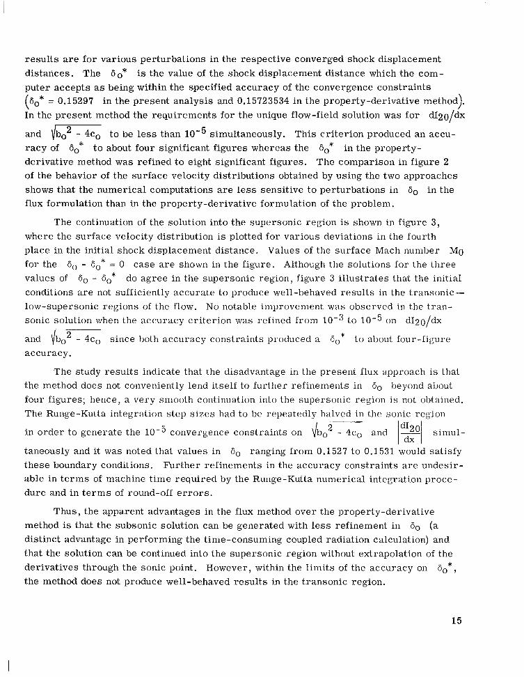
resul ts are for various perturbations in the respective converged shock displacement distances. The 60* is the value of the shock displacement distance which the computer accepts as being within the specified accuracy of the convergence constraints (60* = 0.15297 in the present analysis and 0.15723534 in the property-derivative method). In the present method the requirements for the unique flow-field solution was for dI2o/dx

and (bo2 - 4c0 to be less than simultaneously. This criterion produced an accuracy of 60* t o about four significant figures whereas the 60* in the property- derivative method was refined to eight significant figures. The comparison in figure 2 of the behavior of the surface velocity distributions obtained by using the two approaches shows that the numerical computations are less sensitive to perturbations in 6, in the flux formulation than in the property-derivative formulation of the problem.

The continuation of the solution into the supersonic region is shown in figure 3, where the surface velocity distribution is plotted for various deviations in the fourth place in the initial shock displacement distance. Values of the surface Mach number Mo for the 6 , - 60* = 0 case a re shown in the figure. Although the solutions for the three values of - 60* do agree in the supersonic region, figure 3 illustrates that the initial conditions a r e not sufficiently accurate to produce well-behaved results in the transonic- low-supersonic regions of the flow. No notable improvement was observed in the transonic solution when the accuracy criterion was refined from to on dI2o/dx

and ibo2 - 4c0 since both accuracy constraints produced a 60* to about four-figure accuracy.

The study results indicate that the disadvantage in the present flux approach is that the method does not conveniently lend itself to further refinements in 6o beyond about four figures; hence, a very smooth continuation into the supersonic region is not obtained. The Runge-Kutta integration step sizes had to be repeatedly halved in the sonic region

in order to generate the convergence constraints on {bo2 - 4c0 and 121 simul-

taneously and it was noted that values in 6 , ranging from 0.1527 to 0.1531 would satisfy these boundary conditions. Further refinements in the accuracy constraints are undesir- able in terms of machine time required by the Runge-Kutta numerical integration procedure and in terms of round-off e r r o r s .

Thus, the apparent advantages in the flux method over the property-derivative method is that the subsonic solution can be generated with less refinement in So (a distinct advantage in performing the time-consuming coupled radiation calculation) and that the solution can be continued into the supersonic region without extrapolation of the derivatives through the sonic point. However, within the limits of the accuracy on fj0*,

the method does not produce well-behaved results in the transonic region.

15

It should be noted that Belotserkovskii (ref. 5) recommends a hybrid procedure, wherein the unknown init ial parameters are refined, and the solution advanced by using the property derivative equations. When the regularity condition at the sonic point is satisfied to the specified accuracy, the flux equations are used to pass through and beyond the sonic point.

Figures 2 and 3 are for the perfect gas model, but about the same techniques can be used for equilibrium air to generate similar results. It should be noted that no convenient algebraic expression is available for uo for the equilibrium air model and thus the analysis requires either an extrapolation of uo into the supersonic region or the selec- tion of the proper values of the surface properties which wil l yield velocities greater than sonic just beyond the sonic point.

RESULTS AND DISCUSSION

The results of the numerical approach to the blunt-body flow-field solution are presented here. The solutions are applicable for the inviscid adiabatic steady flow of a perfect gas or equilibrium air over a spherical body.

Flow-field results are presented for the perfect gas model at a free-s t ream pres- su re of 0.01 atmosphere, a density of 1.562 X gram per cubic centimeter, and a specific heat ratio of 1.4 at free-stream Mach numbers of 5.017, 10.0, and 16.6. The equilibrium air cases which are examined are as follows:

Case I: Ub, = 4.572 X l o5 cm/sec (15 000 ft/sec); altitude = 45.72 km (150 000 f t )

Case 11: Ub, = 9.144 X l o 5 cm/sec (30 000 ft/sec); altitude = 45.72 km (150 000 ft)

Case 111: Ub, = 1.3714 X l o 6 cm/sec (45 000 ft/sec); altitude = 60.96 km (200 000 ft)

A resume of the free-stream conditions and the results for each of the perfect gas and the air cases are given in tables I and 11, respectively.

Flow-field results are compared with the results of the inverse flow-field programs of Marrone (ref. 12), Garr and Marrone (ref. 13), Lomax and Inouye (ref. 14), and Inouye (ref. 10); with the results of a property-derivative method solution obtained by J e r r y C. South of the Langley Research Center; and with the experimental data of Sedney and Kahl (ref. 15).

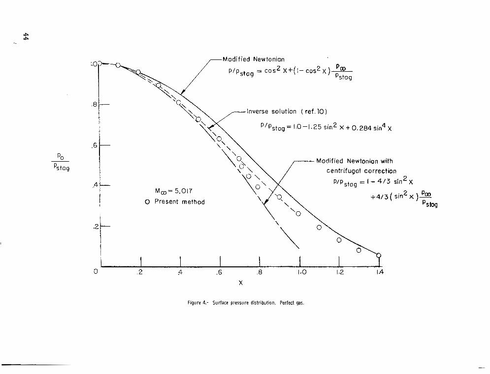
Perfect Gas Results

Property distributions -~ along the body surface.- The body surface pressure distribution for the M, = 5.017 case is shown in figure 4 in both the subsonic and supersonic

16

flow regions. The pressure distributions predicted by "modified" Newtonian theory with and without the centrifugal correction are plotted for comparison. The two modified Newtonian theories tend to bracket the data obtained by the present method. In the subsonic region, the present results for the sphere tend to agree more closely with the centrifugal correction theory. Also shown in figure 4 is the pressure distribution which was correlated from the inverse-flow-field solution. (See refs. 10 and 14.) As evidenced by the f igure, the pressures agree very well with the inverse correlation except near the sonic point. The disagreement in the pressures in the transonic region (x =: 0.7 to 0.8) is associated with the limited three to four place accuracy of 60* and, as previously mentioned, this accuracy is not sufficient to produce well-behaved results near the singularity.

The surface velocity and pressure results of the three perfect gas cases are shown

in figures 5 and 6, respectively. The accuracy criterion of dbo2 - 4c0 5 and d120/dx 5 10-3 was required in the M, = 10.0 and M, = 16.6 solutions. The pres- su res in the subsonic region are of acceptable levels; however, in the supersonic region for the M, = 10.0 and M, = 16.6 cases , the pressures are obviously too low since they become negative on the sphere. The surface velocities are correspondingly too high. It is further evident in figure 6 that the surface pressures obtained in the present analysis are lower in the supersonic region than the experimental values (ref. 15) for the sphere at M, = 5.017 and are lower than both the one-strip property-derivative results M, = 5.017, y = 1.4 and the two-strip results of Belotserkovskii (ref. 5) for M, = 10.0, y = 1.4.

Shock and body shapes.- The stagnation-line shock-displacement distances which were obtained from the three perfect gas cases are shown in figure 7 as functions of the free-s t ream Mach number. Also shown in the figure are the results of the two-strip property-derivative integral method (ref. 16), the results of the inverse solution (refs. 12 and 13), the correlation equation given in reference 10, and the experimental data of reference 15. The shock-displacement distances computed by the present method are within 5 percent of the other results presented in this f igure.

- _-

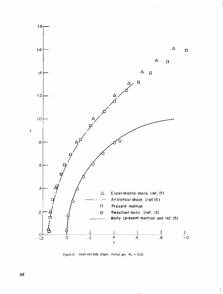
Shown in figures 8, 9 , and 10 are the shock shapes which were obtained in the present approach for M, = 5.017, 10.0, and 16.6, respectively. For the M, = 5.017 case (fig. 8), a comparison is shown between experimental data (ref. 15) and analytical results of the present method and the inverse method (ref. 13). These data are in good agreement; however, some deviations begin to appear in the transonic region (x =: 0.6). For the M, = 10.0 and 16.6 cases (figs. 9 and lo) , a comparison is shown between resul ts of the present method, results of the two-strip property-derivative integral method (ref. 16), and results of the inverse method (ref. 13). These data also compare favorably but indicate some deviations beginning in the transonic region.

17

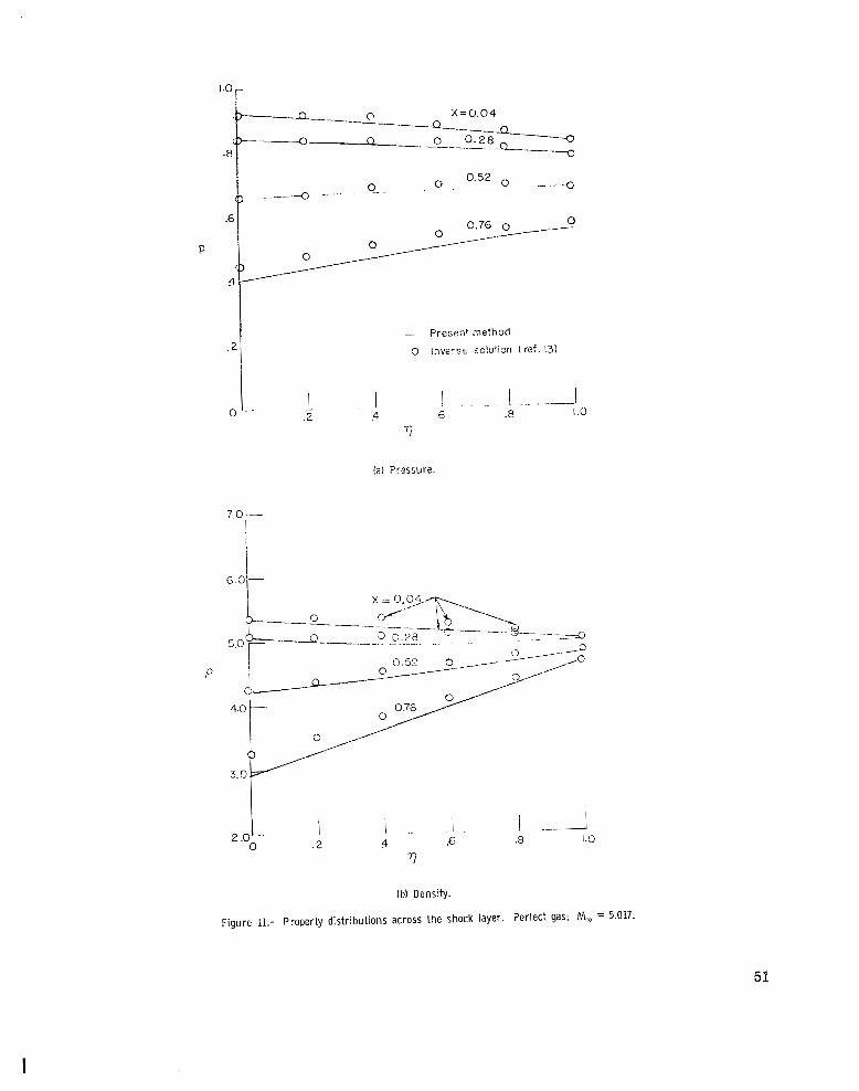
Property distributions across the shock layer.- Comparisons of the properties across the shock layer which were obtained from the present analysis with the results of reference 13 are shown in figures 11, 12, and 13 at various body stations in the subsonic- transonic regions.

Shown in figures l l (a) , l l (b ) , and l l ( c ) are the pressure, density, and resultant velocity distributions, respectively, across the shock layer for M, = 5.017 at x = 0.04, 0.28, 0.52, and 0.76 radian. The flow is subsonic at the x = 0.52 and lower and is in the transonic region at x = 0.76 (Mo = 1.1). The property distributions across the shock layer agree with the inverse solution to within 2 to 3 percent in the subsonic region. At x = 0.76, the present solution gives properties near the body (7 = 0 and 0.2) which deviate from those obtained from the inverse solution by approximately 10 percent. This disagreement is associated with the sonic singularity problem as mentioned previously.

The property distributions across the shock layer at M, = 10.0 and 16.6 a r e shown in figures 12 and 13, respectively, for various locations in x. As in' the M, = 5.017 case, the pressure, density, and resultant velocity are within 2 to 3 percent of the inverse solution values in the subsonic region. In the transonic-supersonic region, x = 0.76 and x = 0.73 at M, = 10.0 and M, = 16.6, respectively, the body surface propert ies are within about 10 percent of the inverse-solution values.

Since the inverse solution is restricted to the subsonic-transonic regions of the flow field, no comparisons of the properties distributions were made in the supersonic regions with this method.

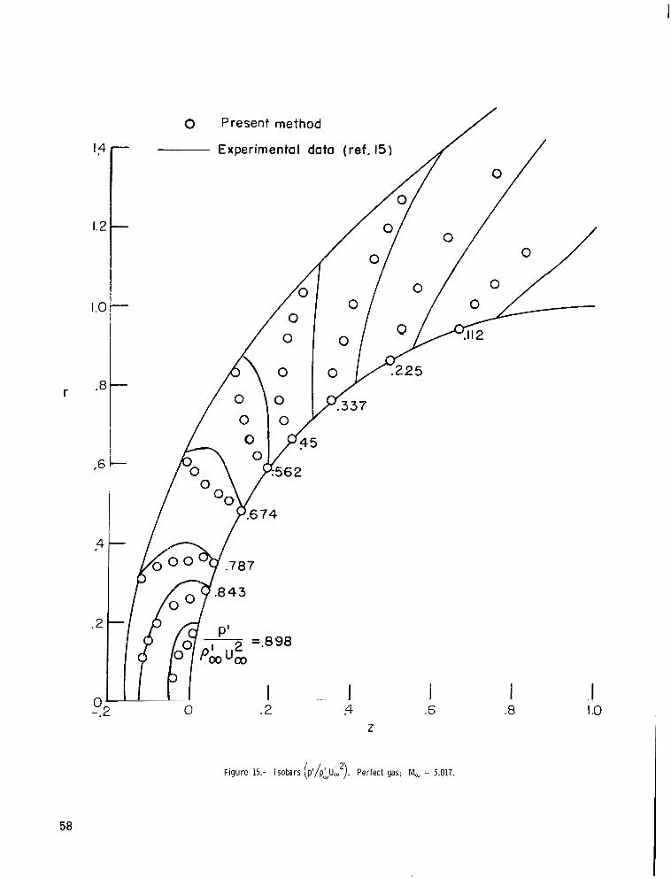
Comparisons of the density and pressure results which were obtained by the present approach in both the subsonic and supersonic regions with the experimental results of reference 1 5 a r e shown in figures 14 and 1 5 for the M, = 5.017 case. There appears to be some disagreement in the densities obtained from the experimental data (ref. 15) and the present method as shown in figure 14. However, it should be noted that the shape and location of the constant density curves are extremely sensitive to the density values, particularly in the stagnation region. (Observe the character and location of the curves for pf/pb, = 5.0 and pf/p, = 4.8 where the difference in the density is only 4 percent.) The largest discrepancies in both the densities and the pressures occur near the body in the supersonic region where the present approach predicts values too low.

Belotserkovskii and Chushkin (ref. 17) recommend in the free-stream Mach number range of 4 to 6 that a second-order approximation to the fluxes is required for an adequate subsonic solution over the blunt body, and above M, = 10 the f irst-order approximation is sufficient. The present analysis indicates that the first-order approximation yields adequate subsonic flow-field results even for the M, = 5.017 case.

18

It is appropriate to note that apparently, the results which one obtains from the integral-relations approach depend somewhat on the choice of the quantities which a r e assumed to vary linearly across the shock layer. For instance, Xerikos and Anderson (ref. 18) indicate that the use of the unaltered continuity equation, as was employed in the present analysis, produces surface pressures which are lower than those obtained from a combined continuity-entropy equation, as was employed in both of the Belotserkovskii analyses (refs. 5 and 16), and lower than experimental data. This effect was not fully investigated in this analysis because the use of the equation for isentropic flow on the body surface p p?' = Constant) is not convenient in an equilibrium air analysis and is not valid for nonadiabatic shock layers (radiating flow fields). However, it was observed in the present analysis, that when the exact x-momentum equation was replaced with the isentropic expression p pY = Constant), the results obtained from the two approaches were identical.

( 1

( 1

Xerikos and Anderson (ref. 18) recommend consideration of the continuity-entropy formulation in equilibrium air analyses; however, this procedure requires an additional correlation (for entropy) and further it is unlikely that this method can be effectively applied to radiating flow-field analyses where the entropy along the body surface is not constant.

Equilibrium Air Results

As mentioned in the analysis section, there are several ways in which stagnation pressures can be generated. The two methods considered here are (1) pstag = p1 + 1 p1v12 approximation and (2) the second derivative approximation,

is otherwise specified, the first approximation for pstag is employed.

Property - distributions along the body.- The body surface pressure distributions for the equilibrium air solutions of cases I, 11, and III are presented in figure 16. The pressure distribution which was correlated by Inouye (ref. 10) from the inverse flow-field solution of reference 14 is also shown in figure 16. The surface pressures for the three cases are within 8 percent of the correlation.

. " "

The surface density distributions for the three cases are shown in figure 17 along with the corresponding density distributions of the inverse solution (ref. 14). Of the three cases examined, a maximum disagreement of 6 percent occurred in the density obtained by the two approaches.

The surface temperature distributions which were obtained in the present analysis are shown in figure 18. The surface pressure results of the inverse solution (ref. 14)

19

were used as inputs to generate surface temperatures in the equilibrium air program of reference 19. These temperatures are also shown in figure 18. The temperatures generated by the present method are within 2 percent of the temperatures obtained by the free-energy minimization approach of reference 19.

Shock and body shapes.- The initial values of the shock-displacement distances for the three cases were found by iterating until three or four significant figures were obtained for the converged value of the standoff distance 60*.

The values of 60* for the three cases are given in table I and are plotted against p,/pl in figure 19, along with the correlation equation of reference 10. The initial shock displacement distances which were generated by the present method are in fair agreement, within about 6 percent, with the shock displacement distances obtained by the inverse solution for cases I1 and 111, as shown in table 11. The case I result for the initial shock displacement distance is 5 percent lower than the displacement distance predicted by the correlation equation of reference 10 and is 9 percent lower than the value of reference 19.

Shown in figures 20, 21, and 22 are the shock shapes which were obtained in the present approach for cases I, 11, and 111, respectively. The results compare favorably with the shock and body-shape results of the inverse solution (ref. 14).

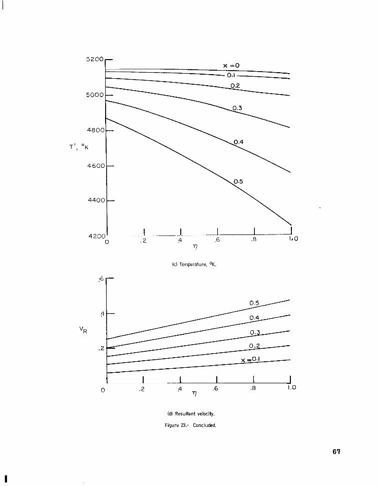
Property distributions ~~~~~ . ~ across - the - shock layer.- The property distributions across the shock layer at various body stations in the subsonic region are shown in figures 23, 24, and 25 for cases I, 11, and 111, respectively. The pressure, density, and resultant velocity distributions of the inverse solution (ref, 14) are also presented for cases I1 and III. A comparison of the results indicates that the pressures and densities obtained from the two approaches agree to within 6 percent. The resultant velocities across the entire shock layer are in excellent agreement for the two cases.

-~ .

Also shown in figures 23, 24, and 25 are the stagnation streamline (x = 0) tempera- tu res which were produced by the equilibrium air program (ref. 19). The temperature results are within 2 percent of the values generated by reference 19.

Stagnation pressure .~ " assumption.- One of the primary advantages of using the second derivative approximation for the stagnation pressure rather than the postshock total- pressure approximation is that the former gives a more accurate value of the stagnation- point velocity gradient which is required to calculate convective heating rates. Kuby, et al. (ref. 7) examined the stagnation-point velocity gradients predicted by the property- derivative method of integral relations and concluded that the method consistently predicted values which were excessively high, The present method predicts stagnation-point velocity gradients which are too high for the postshock total-pressure approximation

."

20

= 0.69 for case whereas the second-derivative approach yields values which

are closer to Newtonian and are more accurate (($)x=o = 0.39 for case

The large differences in stagnation-point velocity gradient however have little effect on the other flow-field results. The pressure distributions obtained by two different stagnation-pressure approximations are shown along with the inverse-solution pressure correlation (ref. 10) in figure 26 for case ID. The pressure distribution is slightly improved when the postshock stagnation-pressure approximation is eliminated in lieu of the second-derivative approximation for 0 = -2.5. The values of 60* for the three cases increased about 4 percent for the latter approximation and thus improved slightly in comparison with the inverse-solution results. About the same percentage changes were noted in the other fluid dynamic and thermodynamic properties.

CONCLUDING REMARKS

A modified method of integral relations approach for a first-order approximation of the fluxes has been used to study the inviscid adiabatic blunt-body flow field. Perfect gas and equilibrium air models are considered in the analysis of the flow over spheres.

The study results indicate that the modified method of integral relations produces subsonic solutions in which the shock displacement distance, the shock shape, and the thermodynamic and fluid dynamic properties throughout the shock layer are in good agreement with the results of the inverse solutions and with experimental data.

The solution generated near the sonic singularity is somewhat less sensitive to the accuracy on the initial shock displacement distance 6 , in the flux formulation than in the standard or property-derivative formulation of the method. The results of the perfect-gas analysis demonstrate that in the modified method of integral relations approach, a convergent supersonic solution was obtained with about four significant figures for the initial value of the shock-displacement distance. However, the present approach predicts surface pressures which a r e low in the supersonic region. Xerikos and Anderson's numerical results indicated that the pressures in the supersonic region could be improved by employing a combined entropy-continuity equation instead of the pure continuity equation as was used in this analysis. In radiating flow-field analyses the combined entropy-continuity approach may have merit in the supersonic region; however, the additional complications are not warranted in subsonic analyses.

21

The equilibrium air flow-field results indicate that the method can be successfully applied to weak radiating flow-field analyses. But, more significantly, the relatively uncomplicated method of integral relations is sufficiently accurate and versatile so that it continues to offer promise for extension to coupled radiating flow-field analyses.

Langley Research Center, National Aeronautics and Space Administration,

Langley Station, Hampton, Va., July 18, 1969.

22

APPENDIX A

DEVELOPMENT O F THE GOVERNING DIFFERENTIAL EQUATIONS

The general governing differential equations which were developed in the analysis section (eq. (11)) were written in the form:

These relations were obtained by integrating the governing equation (eq. (8)) over the shock layer and then performing the necessary differentiations with respect to x.

For the one-strip approximation, equation (8) is integrated once from the body ( q = 0) to the shock ( q = 1) to yield:

Interchanging the order of integration and differentiation in the first term of equation (Al) and integrating the second term by parts gives

Examining equation (A2) it is seen that integrals of the form lo1 Ijr dq appear where

r = r + 6 c o s O q b ( b) (A3)

and from equation (10)

Ij = 1j0 + (1j1 - 1j0)q ( j = 2 , 3 , 4, 5)

Note that the r t e rm is treated separately from the l inear flux approximation. In some analyses (refs. 1 , 2 , 5, 6 , and 18) , the Ij and r a r e "lumped" together as one linear approximation across the shock layer that is, Ijr = IjOrb + (Ijlrl - Ijorb)q).

Now defining

substituting equations (A3) and (10) into the preceding equation, and performing the quad- rature yields

23

APPENDIX A

Now, defining (see eq. (A2))

and expanding equation (A4) gives

Differentiating the right-hand side of equation (A5) gives

The first term in equation (A2) can now be replaced by its equivalent d Pj)/d., and becomes:

(

Substituting the expression for d P. dx (eq. (A6)) into equation (A7), evaluating the remaining terms in these expressions, and combining like terms yields

( 3)/

Equation (A8) can now be written in the desired form:

24

APPENDIX A

when it is noted that

thus, the coefficients of the governing differential equations become

J An examination of the Ej coefficients reveal that terms of the form 66 J" Kj dq

appear. These terms may be evaluated from the Kj expressions of equation (9): 'b 0

K2 = 0

Replacing p with its equivalent I3 - pu2 gives

25

I

APPENDIX A

The K- expressions can be immediately integrated upon assuming a linear variation for ~ u 2 across the shock layer. The Kj terms yield

1

66 j" 36 drb 6 Sin ob

'b 0 %(I30 + ' 3 l ) Z rb

2 - K3 dq = - + (I30 2 1 3 1 ) z 'b + 6Q(3 + 26 cos rb ob )41

36 drb 6 2 . Sln ob 'b

Thus

(Equations continued on next page)

26

APPENDIX A

2S2Q COS 8b 36 cos 8b

'b (I30 + 2131) 'b (pouo2 + P1U12)

where

27

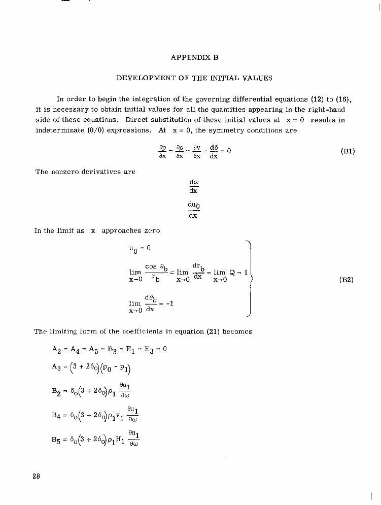
APPENDIX B

DEVELOPMENT OF THE INITIAL VALUES

In order to begin the integration of the governing differential equations (12) to (16), it is necessary to obtain initial values for all the quantities appearing in the right-hand side of these equations. Direct substitution of these initial values at x = 0 results in indeterminate (O/O) expressions. At x = 0, the symmetry conditions are

The nonzero derivatives are dw dx I

In the limit as x approaches zero

uo = 0 7 cos ob drb

l im -- - l im dx = l im Q = 1 x-0 'b x-0 x-0

deb lim - = -1

The limiting form of the coefficients in equation (21) becomes

A2 = A4 = Ag = B3 E1 = E3 = 0

A3 = (3 + 26o)(Po - PI)

28

APPENDIX B

E4 = 6,(3 + 26,)p1v1 2 + 2(3 + 36, + 6,2)(po - p + (6 + 96, + 4602)pl~12 1)

where

From the y-momentum equation (eq. (13))

lim - dw = l im (- 2) x-0 dx x-0

Substituting these expressions for E4 and B4 yields

In a similar manner, the continuity equation (14) yields

and, the energy equation (16) gives

6,(3 + 26,)plH1 &l dx dw + (3 + 360 + 602)plv1H1 + 3 6 , R ~ ~-

29

APPENDIX C

A CORRELATION OF EQUILIBRIUM AIR PROPERTIES TO 15 0000 K

By G. Louis Smith and L. Bernard Garrett Langley Research Center

In order to compute the thermodynamic properties of high temperature equilibrium air (or any other mixture of reacting gases) from basic principles, it is necessary to specify the pressure and temperature. If these two variables are known, the composition, density, enthalpy, etc., may be determined directly. Frequently, in flow-field studies the enthalpy and density are given, and it is required to determine pressure and temperature. In order to accomplish this calculation rigorously, it is necessary to resor t to a double iteration whereby through some numerical process one seeks the pressure and tempera- tu re which corresponds to the given enthalpy and density. This procedure is rather lengthy and in flow-field studies, where differential equations must be integrated by using the results of the computations, the thermodynamics computations may take an excessive amount of computer time.

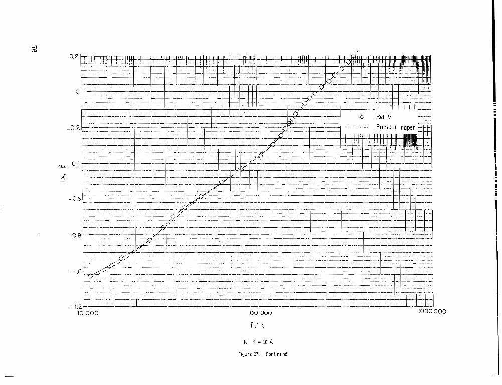
This problem can be alleviated by use of correlation formulas expressing pressure and temperature in terms of enthalpy and density. These formulas are developed from the data of Hilsenrath and Klein (ref. 9) which is used as a standard for thermodynamic data. Correlation formulas have been written expressing the pressure, compressibility, and temperature of equilibrium air as a function of density and enthalpy, for a density ratio p'/PEef range of lom4 to 10 and temperatures up to 15 OOOo K. The pressure is correlated to about 5-percent accuracy, the compressibility about 2 percent to 5 percent, and the temperature to about 10 percent, although through most of the range the accuracy is better than these values.

The approach taken is to express the equation of state of the mixture in the form:

6 = 86,fi) (C1)

The quantities with circumflexes 6, b , and 6 which are used in this appendix are defined as follows:

30

APPENDIX C

.. h'Wref h=-

R' so that for conversion to the nondimensional values used in the text

For many purposes, the relation (Cl) is all that is required. If temperature and/or mean molecular weight are required, the following relations are used. The compressibility Z defined by - *...

is correlated in the form

z = Z(j5,h)

The temperature T' (OK) is then given by

For the correlation for 6(;,f1), the enthalpy range 0 < < 600 OOOO K was divided into five regions as follows:

L

Region I: 0 < h 5 5800° K, or approximately 0 < T' < 1500° K. Within this region air is calorically perfect for practical purposes, and

6 = (0.97513 X 10-3)66 (C 5)

Region 11: 5800° K < 6 5 10 500° K; or approximately 1500° K < T' < 2500° K. Within this region air is a perfect gas, but vibrational modes are excited and energy invested in the formation of nitr ic oxide is significant. Within this region

6 = (0.345 x 10-2)60.8546 (C6)

For the remaining three regions, the phenomena are much more involved and the explana- tion for the behavior is not obvious. The formulas which were fitted to the data are

31

I

APPENDIX C

Region ID: 10 500° K < & < 35 500' K

+ 0.016<(2.75 - <)loglo 6 - O.O05r(4 - {)(1 + loglo 6) (C7)

where

r = 5 loglo h - 20 (C8)

Region IV: 35 500° K 5 & < 178 000' K

loglo fi = 1.565 + 1.036 loglo f i +. 0.668 loglo - 4.8 + 1.1675 loglo - 4.8)3 (C9)

Region V: 178 OOOo K 5 6 < 600 OOOo K

( 1 (

loglo = -3.015 + 1.036 loglo 6 + 0.95 loglo i; (C10)

These correlations hold for the density range

10- 4 6 /3 5 10

A comparison of the correlation formulas (C5) to (C10) with data from reference 9 is shown in figure 27. The correlation is accurate to about 5 percent or better.

The partial derivatives of the pressure with respect to the density and enthalpy are as follows:

Region I:

a5 = (0.97513 X ah

- ?I? = (0.97513 X aij

Region 11:

Region 111:

.% = 9 k . 1 5 4 5 + [0.0131 + 0.016(2.75 - 25gloglO /3 - 0.005(4 - z y ) ( l + loglo b$ a6 h

32

APPENDIX C

9 = p(1 + <[0.0131 + 0.016(2.75 - <) - 0.005(4 - <'J> 6 , .

86 b

where

< = 5 loglo fi - 20

Region IV:

fi - 4.8) l ah h

A A

$ = 1.036 aP P

Region V: A A

2 = 0.95 P ah h

ai; a; P

A

- = 1.036

For the correlation of Z(b,G), it is first noted that in regions I and I1 air behaves as a perfect gas so that

z = 1.0 (6 < 10 500° K) (C11)

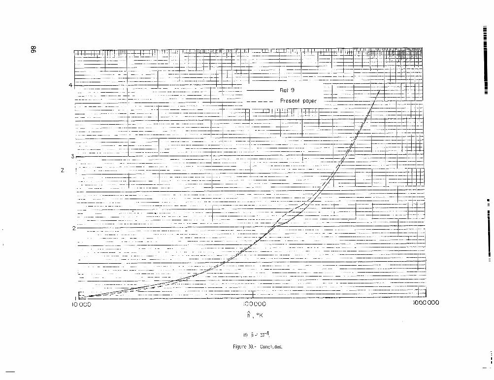
(or approximately T < 2500° K). For higher values of it was found that curves of Z against loglo 6 for constant 6 very nearly coincide when translated horizontally an amount dependent on 6. This relationship is shown in figure 28, where the abscissa is

+ = loglo fi - 0.044 loglo 6 - 0.004 ( loglo 6)2 - 3.952 ( C W

A single curve may thus be used to describe Z. This curve is broken into four regions in order to fit low-order polynomials to it.

Region A : For 6 5 10 500

z = 1.0

Region B: For + 5 0.55

Z = 1.0 + 0 . 5 3 9

Region C: For 0.55 < + < 1.3

Z = 2.0 - 1 . 7 8 ~ + 0 . 2 1 ~ ~ + 1 . 0 9 ~ ~ - 0 . 4 4 6 ~ ~

APPENDIX C

where v = 1.3 - +

Region D: For 1.3 5 < 2.0

Z = 3.831 - 5.019t + 3.41t2 + 0.24t3 (C17)

where

The region $b > 2.0 is outside the range of reference 9, and was not considered in the correlation. The boundaries of these regions are shown in figure 29. The dotted line corresponds to $b = 0.

The results of the correlation formulas (C13) to (C17) a r e shown in figure 30, along with data from reference 9. The comparison is favorable, the error of the correlation being less than 2 percent except in the region 150 000 < 6 < 250 000' K where a 5-percent error occurs.

The temperature is computed from equation (C4) by using the 6 and Z correla- t ions. The error of the temperature correlation is about 10 percent in some places, but is usually less than this amount. (See fig. 31.)

34

APPENDIX D

RANKCNE-HUGONIOT CONDITIONS

The conditions immediately behind the shock are computed from the following Rankine-Hugoniot relations. In the shock-oriented coordinate system (see sketch (a)), these expressions in nondimensional form are:

Shock

Body

For continuity:

For normal momentum:

Sketch (a).- Shock and body-oriented properties.

v m = p v 1 s

For tangential momentum:

u, = us = cos w

35

I

APPENDIX D

For energy:

In the body-oriented coordinate system,

where v1 is defined as positive in the y- or q-direction.

The partial derivatives of the velocity components with respect to the shock angle are required in the analysis. They are:

"- - d u ~ sin(w - ob) + - dVS cos(w - e + us cos w - ob) - vs sin(w - aw d o dw b) (

Perfect Gas Analysis

The perfect gas is characterized by the fact that the ratio of the specific heats y

is a constant. The conditions behind the oblique shock a r e computed explicitly from the following relations:

us = cos w

- 1 2 2 1 +1/" -MM,s in 2 w vs =

M5sin w . "

- li]

36

(Equations continued on next page)

I """, .,"" .,,,. .. -

APPENDIX D

dp1 - 4y PwMm ' 2 " - ~ sin w cos w dw y + l 1 1 2

P,U,

dP1 (y + l )Mwsin w cos w dw

2 "

-

(1 + y+ M:sin

Equilibrium Air Analysis

The expressions in appendix C for equilibrium air thermodynamic properties and the Rankine-Hugoniot relations (eq. (Dl)) are sufficient to compute the properties immediately behind the shock. A Newton-Raphson iteration technique is employed t o obtain a convergent solution. The derivatives of the properties are computed from the derivatives of the governing Rankine-Hugoniot equations and the equilibrium air-pressure correlations.

dpl - "

dw

- = s i n d h l w cos w dw

dpl - = 2 s in w cos w dw

The expressions for 3pl/ahl and apl/8pl a r e obtained from the equilibrium air- pressure correlations and are given in appendix C.

37

II I

REFERENCES

1. Belotserkovskii, 0. M.: Flow Past a Circular Cylinder With a Detached Shock. RAD-9-TM-59-66 (Contract AF04(647)-305), AVCO Corp., Sept. 30, 1959.

2. Traugott, Stephen C.: An Approximate Solution of the Supersonic Blunt Body Problem for Prescribed Arbitrary Axisymmetric Shapes. RR-13, Martin Co., Aug. 29, 1958.

3. Lun'kin, Iu. P.; Popov, F. D.; Timofeeva, T. Ia; and Lipnitzkii, Iu. M.: Passage Through Singularities in the Numerical Solution of Problems of Supersonic Flow Around Bodies. Trudy Leningrad Politekhn. Inst., no. 248, 1965, pp. 7-13.

4. Kao, Hsiao C.: A New Technique for the Direct Calculation of Blunt-Body Flow Fields. AIAA J., vol. 3, no. 1, J a n . 1965, pp. 161-163.

5. Belotserkovskiy, 0. M.: Supersonic Gas Flow Around Blunt Bodies - Theoretical and Experimental Investigations. NASA TT F-453, 1967.

6. Xerikos, J.; and Anderson, W. A.: A Critical Study of the Direct Blunt Body Integral Method. SM-42603, Missile & Space Syst. Div., Douglas Aircraft Co., Inc., Dec. 28, 1962.

7. Kuby, W.; Foster , R. M.; Byron, S. R.; and Holt, M.: Symmetrical Equilibrium Flow Past a Blunt Body at Superorbital Re-Entry Speeds. AIAA J., vol. 5, no. 4, Apr. 1967, pp. 610-617.

8. Dorodnitsyn, A. A,: On One Method of Numerical Solution of Certain Nonlinear Problems of Aerohydrodynamics. UCRL-Trans.-993(L), Lawrence Radiat. Lab., Univ. of California, Sept. 1963.

9. Hilsenrath, Joseph; and Klein, Max: Tables of Thermodynamic Properties of Air in Chemical Equilibrium Including Second Virial Corrections From 1500° K to 15,0000 K. AEDC-TR-65-58, U S . Air Force, Mar. 1965.

10. Enouye, Mamoru: Blunt Body Solutions for Spheres and Ellipsoids in Equilibrium Gas Mixtures. NASA TN D-2780, 1965.

11. Garrett, Lloyd Bernard: A Modified Method of Integral Relations Approach to the Blunt Body Flow Field. M.S. Thesis, Virginia Polytechnic Institute, Aug. 1967.

12 . Marrone, Paul V.: Inviscid, Nonequilibrium Flow Behind Bow and Normal Shock Waves, Part I. General Analysis and Numerical Examples. Rep. No. QM-1626-A-12(1) (Contract No. DA-30-069-ORD-3443), Cornel1 Aeron. Lab., Inc., May 1963.

38

13. Garr , Leonard J.; and Marrone, Paul V.: Inviscid, Nonequilibrium Flow Behind Bow and Normal Shock Waves, Part 11. The IBM 704 Computer Programs. Rep. No. QM-1626-A-12(11) (Contract No. DA-30-069-0~-3443), Cornel1 Aeron. Lab., Inc., May 1963.

14. Lomax, Howard; and Inouye, Mamoru: Numerical Analysis of Flow Propert ies About Blunt Bodies Moving at Supersonic Speeds in an Equilibrium Gas. NASA TR R-204, 1964.

15. Sedney, R.; and Kahl, G. D.: Interferometric Study of the Blunt Body Problem,. Rep. No. 1100, Ballistic Res. Lab., Aberdeen Proving Ground, Apr. 1960.

16. Belotserkovskii, 0. M.: Calculation of Flow Around Axisymmetric Bodies With a Detached Shock Wave (Raschet obtekaniya osesimmetrichnykh tel s otoshedshey udarnoy volnoy). Computer Center Acad. Sci. (Moscow), 1961.

17. Belotserkovskii, 0. M.; and Chushkin, P. I.: The Numerical Method of Integral Relations. NASA TT F-8356, 1963.

18. Xerikos, J.; and Anderson, W. A.: An Experimental Investigation of the Shock Layer Surrounding a Sphere in Supersonic Flow. AIAA J., vol. 3, no. 3 , Mar. 1965, r~p . 451-457.

19. Zoby, Ernest V.; Memper, Jane T.; and Jachimowski, Casimir J .: Isentropic Flow Solutions for Reacting Gas Mixtures in Thermochemical Equilibrium. NASA TN D-4114, 1967.

39

Case

I 11

111

TABLE 1.- RESUME OF PERFECT GAS SOLUTIONS

[All quantities are nondimensional; y = 1.4 " . .

60* M,

I Present method I (a)

5.017 0.9229 5.448 .9228 6.169

16.6 .9209 6.331

~

0.15297 .12902 .12461

I

0.157235 .135240 .130691

Refs. 12 and 13

0.1455 .121 .120

aunpublished data by J e r r y South at Langley Research Center.

TABLE 11.- RESUME O F EQUILIBRIUM AIR SOLUTIONS

[All quantities are nondimensional except as noted 3 7 . .

Free-stream conditions . -

1 I I _ I

Case Altitude, I 1 km 1 atm PL,

gm/cm3 1.

1.445 45.72

.3152 .2226 111 60.96 1.837 45.72 1.837 X 1.445 X

I .

~. . . ~ .

~~ . -

Stagnation conditions

Pstag

0.9577 .9690 .9699

Present method ~= "

Pstag p k t a g ' OK _ _ _ ~

11.28 8 964 16.09 5 113

13 468 16.86

~~ ..

~

60*

0.06568 .04793 .04458

Inverse solution (ref. 14)

.. -

Pstag 1 Pstag I 60* - .. .

0.9591

.0475 17.20 .9708

.0495 16.29 .9701 0.0721 11.34

"

I

Ub,, cm/sec

4.572 X l o 5 9.144

13.72

Free energy minimization (ref. 19)

Pstag Pstag

0.9659 1 11.39 .9773 16.50

.9775 1 17.29

Tktag' OK

5 024 8 826

13 586

40

I

Figure 1.- Flow-field coordinate system.

4 1

r

"0

0' I . 1 I I I I I I I

.I .2 .3 4 .5 .6 .7 .€I X

Figure 2.- In i t ia l -va lue sens i t iv i ty study - subsonic behavior. Perfect gas.

MO .9 1.0 1.1 1.2 1.3 1 . 4 1.6 I .8 2.0 2.2 24 .9" I I I 1 I I I I I 1

M a = 5.017, 7 = 1.4

80 = 0.15297 3rc

" 0

.51-

I I I I I I I 1 .6 .7 .8 .9 1.0 1 . 1 I .2 I .3 I ,4

x

Figure 3.- Ini t ial-value sensit ivi ty study - supersonic behavior. Perfect gas.

.

M,= 5.017

0 Present method

X

x ) P o 0 Ps tag

X

Figure 4.- Surface pressure distribution. Perfect gas.

1.0 -

"0

? -

,6 .8 I .o 1.2 I 0 4 X

Figure 5.- Surface velocity distributions. Perfect gas.

0 Experimental data (ref. 15) ;

Q I -strip solution ( property-derivative Moo = 5.017

in teqra l method of South at L R C ) ; M, = 5.017

4 ;--

“ 10.0

2 ’--

i

Figure 6.- Surface pressure distributions. Perfect gas.

.18 :- I.

;

.I4 -

‘I

0

B

a

Present method

Refs, 12and 13

R e f - 15

r 8 0 = Oe7* - Po0 PI

0

0 0

I I 1 I I .IO L 4 6 8 IO 12 14 16 18

Figure 7.- Variation of shock displacement distance with Mach number. Perfect gas.

1.e

I .6

I P

I .2

I .o

r

.8

.6

9

.2

0

* n

-. 2 0 . 2

Experimental shock (ref. 15)

Analytical shock (ref. 13)

Present method Resultant body (ref. 13) Body (present method and ref. 15)

1 I ! ,4 6 .8 z

_I I .o

Figure 8.- Shock and body shapes. Perfect gas; M, = 5.017.

48

I . €

I P

1.2

1 . 0

r

.6

4

.2

/

/ x u

/"--

. . . . " nnalyr lcol SnoCk ( re t , 13,

- 0 Shock - present method

0 Resultant body (ref. 13)

Body - present method

X - Shock- 2 strip'lproperty derivative"

Z


49

I

_I -- Analyfical shock ( r e f . 13 1 U Shock - present method

0 Resultant body (ref. 13) "- Body - present method

X - Sho& -2 strip "pro9erfy-derivative" integral rnethod(ref. S6) M, =OD

0 ,4 .6 z

.8 1.0


50

r

.2

0 I . 2

" Present method

0 Inve r sE Solution (ref. 13)

7 0 - I

6.0 - I

2.0 - . I 0

I . 2

I - . I 9 .6

77

(b) Density.

I "I .8 1.0

F igu re 11.- Property distr ibutions across the shock layer. Perfect gas; M, = 5.017.

51

I

I I I II

"R

52

-4 -

.3 -

0 ,2 p -6 .8 I . 0

rl

(c) Resultant velocity.

F igu re 11.- Concluded.

X =0.04

.8 _a

I 0.52

2t ~ Present method

0 Inverse solution (ref. 13)

I I -I 0 . 2 p .6 .0 I .o

77

m----" 0.76

" . J L

P

2 .o I I I I 0 .2 .4 .6 .8 I. 0

77

(b) Density.

Figure 12.- Property distr ibutions across the shock layer. Perfect gas; M, = 10.0.

53

Presen t method 0 i nve rse solution ( r e f . 13)

(a) Pressure

3.0 - I 1 . 1 1 0 2 f .6

"7

1-1 .E I .o

(b) Density.

F igure 13.- Property distr ibutions across the shock layer. Perfect gas; M, = 16.6.

55

-/ n nq -0

.2 i4 .6 .8 1.0

(c) Resultant velocity.

Figure 13.- Concluded.

56

I 9

1.2

I .c

r .€I

,6

4

,2

r

0

Figure 14 -

.2 -4 .6 .8 1.0 Z

Constant density prof i les (p'/pL). Perfect gas; M, = 5.017.

57

‘ 4

I. i

1.c

r .E

,E

p

.2

/

0 .2 p I i

.6 .8 Z

I . I ..

I .o

Figure 15.- Isobars (pq/pLUL2). Perfect gas; M, = 5.017

58

Inverse solution ( re f . 10) Po/Pstag = 1.0- 1.25 sin2 X +0.284 sin 4 X

- Present method :

0 Case I A Case r[ B Case III -

.. I I I 0 .I .2 - 3 .4 .5 .6

X

Figure 16.- Surface pressure distributions. Equitibrium air.

18

.16.

14

P 12

10

8

6 0

. ~ .“ -

-

-

-

Inverse solution ( r e f . I4 1 0

Present method : - 0 Case 1

A Case II Case JII

C

. I .2 .3 .4 X

.5 .6

Figure 17.- Surface density distributions. Equilibrium air.

60

14,000 -

12,oo

8000

6000

4 000

Present method 0 Ref. 19

0 0 II 0 0 0

Case I u V - 0 0

U "77

$ 2 .4 .5 .6

Figure 18.- Surface temperature distributions. Equil ibrium air.

Present method

I 0 .04 .O 8 . I2 .I 6 .20

pa 1 p,

Figure 19.- Shock displacement distance a t axis of symmetry. Equi l ibr ium air .

62

;6

.5

.4

r .3

.2

. I

C

/ /

I b I I

" P I I

" b C>

I

-

" Analytical shock (ref . 14 Shock - Present method

0 Resultant body (ref. 14 )

B o d y - present method

1 " 0 - I I .2 . 3

Figure 20.- Shock and body shapes. Equilibrium air; case I.

63

I

;E

c - *

.4

r .3

.2

. I

0

I

0

Analytical shock ( re f . 1 4

Shock -present method Resultant body ( re f . 14 )

Body -present method

-. I 0 . I . 2 .3 2

Figure 21.- Shock and body shapes. Equilibrium air; case I I .

64 I

.6

.5

4

r

. 3

.2

. I

" Analytical shock ( r e f . 14) -

0 Shock -present method

0 Resultant body (ref. 14)

Body - present method I I

- P I

0 .I .2 2

.3

Figure 22.- Shock and body shapes. Equilibrium air; case I l l

65

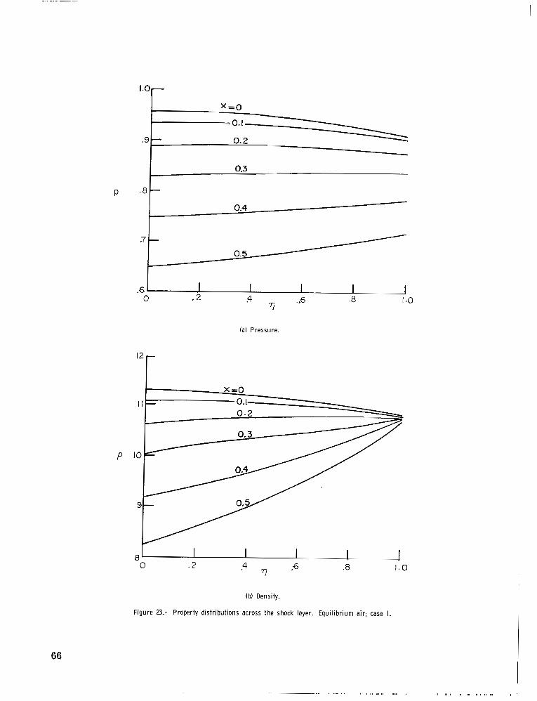
.9 t 0.3

P

.6 I I 1 1 1 1 77

0 .2 .4 . .6 .0 I .o

(a) Pressure.

0 .2

0.3

IO

8 I 1 1 1 1 0 . 2 4 ,G .8 1.0

' 7 7

(b) Density.

Figure 23.- Property d istr ibut ions across the shock layer. Equi l ibr ium air ; case I.

66

. . . . . .. _... ...

520C

5ooc

480(

T ' , O K

460(

440(

4 20(

- x =o .. -

0. I

(c) Temperature, OK.

r P -

"R

.2

I I I I I I 0 .2 9 .6 .E? I .o

7 )

(dl Resultant velocity.


I

n 0"

R 1 0.2 0

.. -_______D

.9 - 1 0.3 0 0

P 0

.8 - 0.4 0 - A

.7 1 - A Present method

0 Inverse solution (ref. 14)

I 1.0

P

'I

(a) Pressure.

X = 0.5-

1 .E

I I .o

(b) Density.

F igu re 24.- Property distr ibutions across the shock layer. Equil ibr ium air; Case 1 1 .

68

I

9000

8600

T ' , O K

8 2 0 0

.6

.4

VU

.2

2 9 -6 rl

(c) Temperature, OK.

.8 1.0

0 .2 9 .6 - 8 1.0

77

Id) Resultant velocity.

F igu re 24.- Concluded.

69

P

I o inverse solution (ref. 14)

77

(a) Pressure.

/

(b) Density.

F igu re 25.- Property distributions across the shock layer. Equil ibr ium air; case Ill.

70

14000r

T: "K

13500,- li. ""

0 L.

.." 0. I .. " - - 0.2 ", -

13000

12500 -

I2000 - 17 ( Ref. 19 at x = 0 )

li. ""

X 13500,- .." u

.. " - 13000

I I500 I 0

I .2

I I p

rl .6

I 1 -8 I .o

(c ) Temperature, OK.

0 .2 4 -6 .8 1.0 . 7 7

(dl Resultant velocity.

F igure 25.- Concluded.

71

PO

%tag

1.0

.9

.8

.7 "- Pstog-P,+ - i P , I v approximation

"- Pstag= I ( dd?xp2) P

approximation , p = - 2,5 x = o

P/P,tag = 1.8-1.25 sin 2 X + 0.284 sin4)(

.5' I I I 0 , 1 -2 .3 -4 .5

X

Figure 26.- Comparison of pressure distr ibution for dif ferent stagnation pressure approximations. Equil ibr ium air; case Ill.

0'0 "~"""""""-I " L* _I ........................... ...

-. I ............... ........... ............ .................. ~ -~

"~ ___ 1 L I I L I W ___ "" " "_ " "_. -

6."' ~

10 000 IOQ 000 h , "K A

( a ) p^ = 10.

Figure 27.- Pressure as a function of ^h for constant density 6.

IO00 000

Figure 27.- Continued.

A h , O K


0 -2

0

, $ , O K


4 4 Figure 27.- Continued.


4.0 -

Data from reference 9

""_ Curve f i t z ( $ 1

Figure 28.- Compressibility Z as a funct ion of #.

4 W

E

5

log h A

4

7

A h too large

- 1 Region D

Region C

Region A

3 2 0 -- 2 -4

, I -6

Figure 29.- Regions of applicabil ity of compressibi l i ty correlat ion Z.

80

Figure 30.- Compressibility 2 as a funct ion of enthalpy h for constant density p .

m N


IO 000 l000rJ00

( c ) 6 = !0-1.

Figure 30.- Csni iwed.

4

Z



IO 000 ~00000 1000000 n h , O K

Figure 30.- Concluded

Temperature as a function of enthalpy ^h for a constant density p .

T

" IO 000 l00000 1000

Figure 31.- Continued,

000

T

10000 100 0 00 1000 000



000


W N

20

-r ' , O K

e (D

(D m

l e N

t? Q, h3 0 W Figure 31.- Concluded.

NATIONAL AERONAUTICS AND SPACE ADMINISTRATION WASHINGTON, D. C. 20546

OFFICIAL BUSINESS FIRST CLASS MAIL

NATIONAL AERONAUTICS AND POSTAGE AND FEES PAID

cP*rT *"MINISTRATION

POSTMASTER: If Undeliverablc (Section 158 Postal M a n u a l ) Do Not Return

NASA SCIENTIFIC AZVD TECH-NICAL PUBLICATIONS

TECHNICAL REPORTS: Scientific and technical information considered important, complete, and a lasting contribution to existing knowledge.

TECHNICAL NOTES: Information less broad in scope but nevertheless of importance as a contribution to existing knowledge.

TECHNICAL MEMORANDUMS: Information receiving limited distribution because of preliminary data, security classificn- tion. or other reasons.

CONTRACTOR REPORTS: Scientific and technical information generated under a NASA contract or grant and considered an important contribution to existing knowledge.

TECHNICAL TRANSLATIONS: Information published in a foreign language considered to merit NASA distribution in English.

SPECIAL PUBLICATIONS: Information derived from or of value to NASA activities. Publications include conference proceedings, monographs, data compilations, handbooks, sourcebooks, and special bibliographies.

TECHNOLOGY UTILIZATION PUBLICATIONS: Information on technology used by NASA that may be of particular interest in commercial and other non-aerospace .lpplications. Publications include Tech Briefs, Ttchnology Utilizuion Reports and Notes, and Technology Surveys.

Details on the availability of these publications may be obtained from:

SCIENTIFIC AND TECHNICAL INFORMATION DIVISION

NATIONAL AERONAUTICS AND SPACE ADMINISTRATION Washington, D.C. 20546

Documents

COPY: KIRTLAND