Embed Size (px)
Citation preview

COP 3502: Computer Science I (Note Set #21) Page 1 © Mark Llewellyn
COP 3502: Computer Science ISpring 2004
– Note Set 21 – Balancing Binary Trees
School of Electrical Engineering and Computer ScienceUniversity of Central Florida
Instructor : Mark Llewellyn [email protected]
CC1 211, 823-2790http://www.cs.ucf.edu/courses/cop3502/spr04

COP 3502: Computer Science I (Note Set #21) Page 2 © Mark Llewellyn
• As we mentioned previously, the run-time of our search algorithm (also insertion and deletion algorithms) is highly dependent on the balance of the BST being searched.
• If the data from which a BST is to be built arrives in sorted order, the resulting tree will be a right skewed tree that will resemble a linear list. The resulting search time will be O(n) rather than the O(log2n) that should be expected.
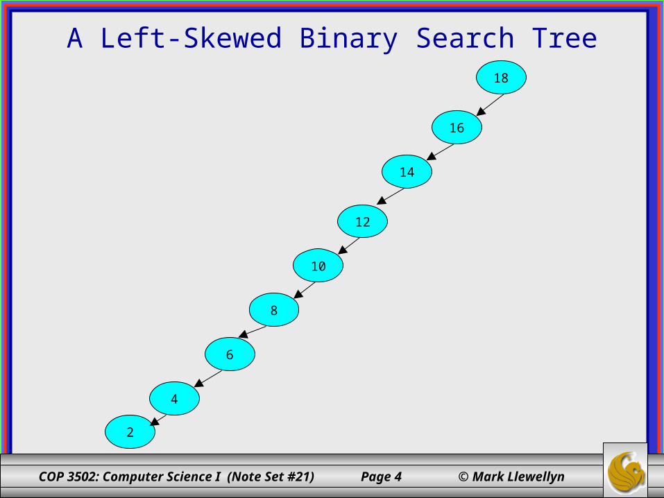
– If the data arrives in reverse sorted order the resulting tree will be left skewed.
• Since the run-time of our algorithms is dependent on the structure property of the BST as well as the ordering property, we need to be sure that the BST is as short and fat as possible rather than tall and skinny.
The Need to Balance Binary Search Trees

COP 3502: Computer Science I (Note Set #21) Page 3 © Mark Llewellyn
A Right-Skewed Binary Search Tree
26
13
24
28
25
22
20
18
16
COP 3502: Computer Science I (Note Set #21) Page 4 © Mark Llewellyn
A Left-Skewed Binary Search Tree
4
18
8
2
6
10
12
14
16
COP 3502: Computer Science I (Note Set #21) Page 5 © Mark Llewellyn
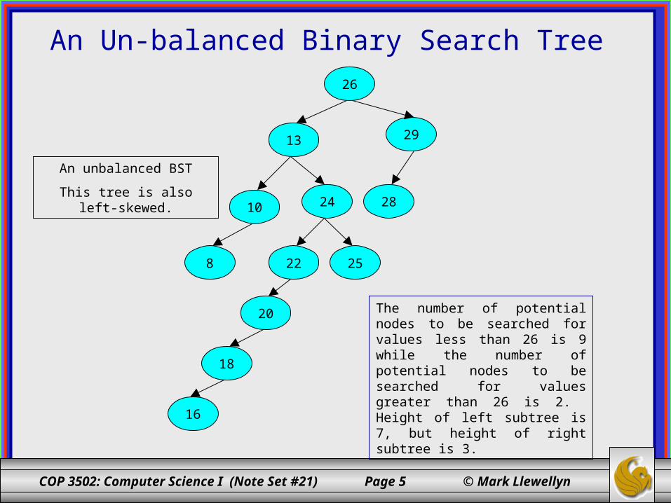
An Un-balanced Binary Search Tree 26
13
24
29
10
8
28
2522
20
18
16
An unbalanced BST
This tree is also left-skewed.
The number of potential nodes to be searched for values less than 26 is 9 while the number of potential nodes to be searched for values greater than 26 is 2. Height of left subtree is 7, but height of right subtree is 3.

COP 3502: Computer Science I (Note Set #21) Page 6 © Mark Llewellyn
• What we need to do is take an un-balanced BST and balance the tree at each subtree level and maintain the search tree ordering property in the process.
Balancing Binary Search Trees
13
22
20
18
16
13 22
20
18
16
Un-balanced BSTBalanced BST
transform into
COP 3502: Computer Science I (Note Set #21) Page 7 © Mark Llewellyn
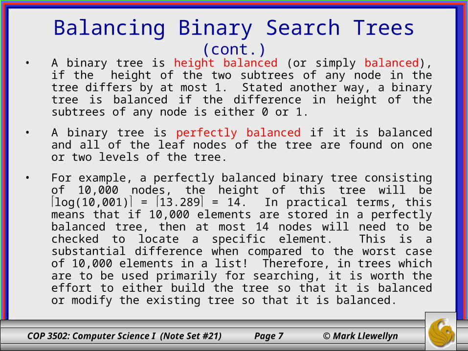
• A binary tree is height balanced (or simply balanced), if the height of the two subtrees of any node in the tree differs by at most 1. Stated another way, a binary tree is balanced if the difference in height of the subtrees of any node is either 0 or 1.
• A binary tree is perfectly balanced if it is balanced and all of the leaf nodes of the tree are found on one or two levels of the tree.
• For example, a perfectly balanced binary tree consisting of 10,000 nodes, the height of this tree will be log(10,001) = 13.289 = 14. In practical terms, this means that if 10,000 elements are stored in a perfectly balanced tree, then at most 14 nodes will need to be checked to locate a specific element. This is a substantial difference when compared to the worst case of 10,000 elements in a list! Therefore, in trees which are to be used primarily for searching, it is worth the effort to either build the tree so that it is balanced or modify the existing tree so that it is balanced.
Balancing Binary Search Trees (cont.)

COP 3502: Computer Science I (Note Set #21) Page 8 © Mark Llewellyn
• There are a number of techniques that have been developed to balance binary trees. Some of the techniques consist of constantly restructuring the tree when elements arrive and lead to a balanced tree. Some of them consist of reordering the data and then build the tree according to some ordering of the data which will ensure that the tree is balanced when it is constructed.
• As we saw earlier, if the data which is used to construct a BST arrives in either ascending or descending order the tree will be skewed to the point of representing a linear list. Thus, if the smallest value in the data set is the first value read, the root of the tree will contain only a right subtree. Similarly, if the largest value in the data set is entered first, the root of the tree will contain only a left subtree. Before looking at more sophisticated algorithms to balance binary trees, lets examine a very simple technique to construct a balanced BST.
Balancing Binary Search Trees (cont.)

COP 3502: Computer Science I (Note Set #21) Page 9 © Mark Llewellyn
• When the data arrive, store all of them into an array. Once all the data have arrived, sort the array using an efficient sorting algorithm.
• Once sorted, the element at the midpoint of the array will become the root of the BST. The array can now be viewed as consisting of two subarrays, one to the left of the midpoint and one to the right of the midpoint.
• The middle element in the left subarray becomes the left child of the root node and the middle element in the right subarray becomes the right child of the root.
• This process continues with further subdivision of the original array until all the elements in the array have been positioned in the BST.
• A slight modification of this would be to completely generate the left subtree of the root before generating the right subtree of the root. If this is done, then the very simple recursive procedure shown on the next slide can be used to generate a balanced BST.
Constructing A Balanced BST
COP 3502: Computer Science I (Note Set #21) Page 10 © Mark Llewellyn
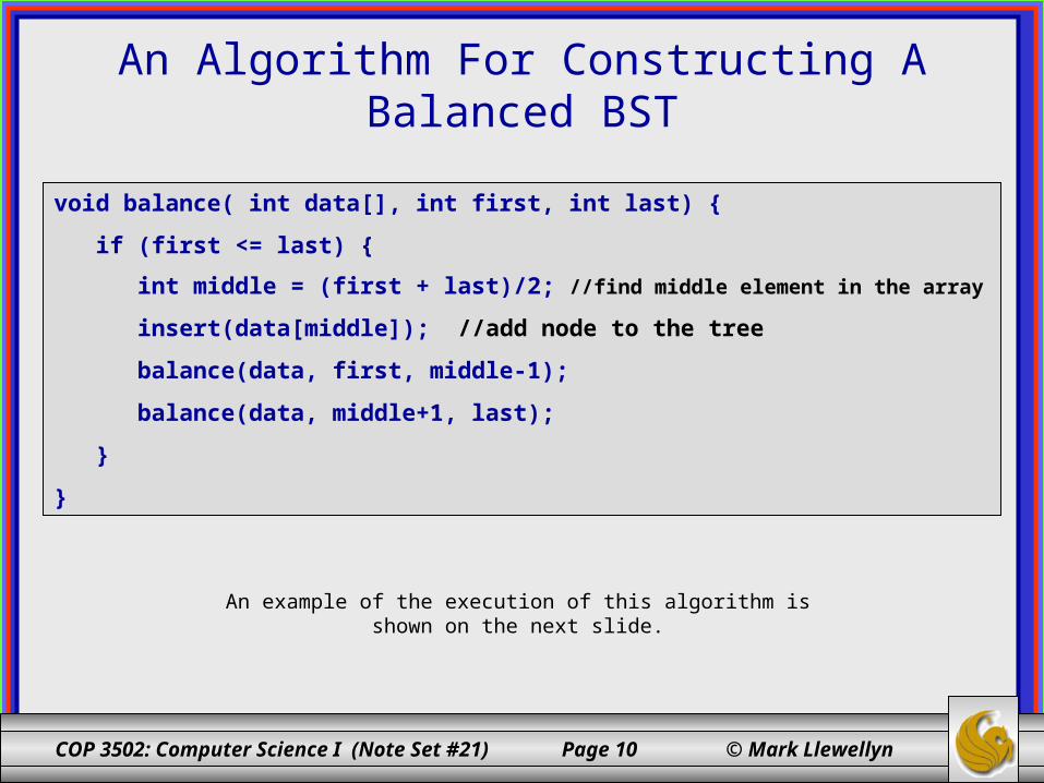
An Algorithm For Constructing A Balanced BST
void balance( int data[], int first, int last) {
if (first <= last) {
int middle = (first + last)/2; //find middle element in the array
insert(data[middle]); //add node to the tree
balance(data, first, middle-1);
balance(data, middle+1, last);
}
}
An example of the execution of this algorithm is shown on the next slide.
COP 3502: Computer Science I (Note Set #21) Page 11 © Mark Llewellyn
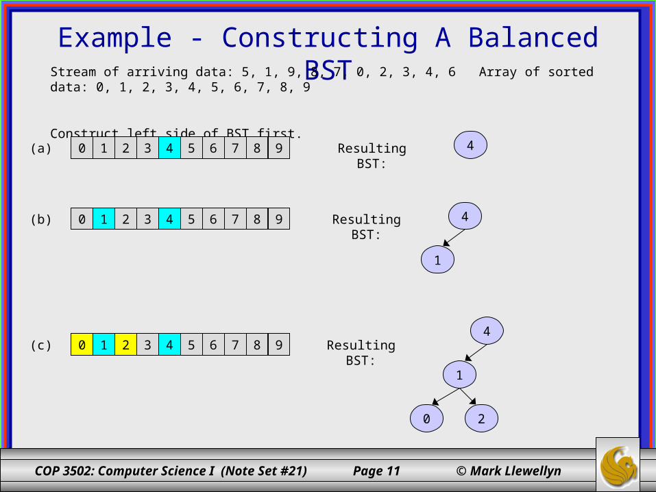
Example - Constructing A Balanced BSTStream of arriving data: 5, 1, 9, 8, 7, 0, 2, 3, 4, 6 Array of sorted data: 0, 1, 2, 3, 4, 5, 6, 7, 8, 9
Construct left side of BST first.0 1 2 3 4 5 6 7 8 9(a)
0 1 2 3 4 5 6 7 8 9(b)
Resulting BST: 4
Resulting BST:
0 1 2 3 4 5 6 7 8 9(c) Resulting BST:
4
1
4
1
0 2
COP 3502: Computer Science I (Note Set #21) Page 12 © Mark Llewellyn
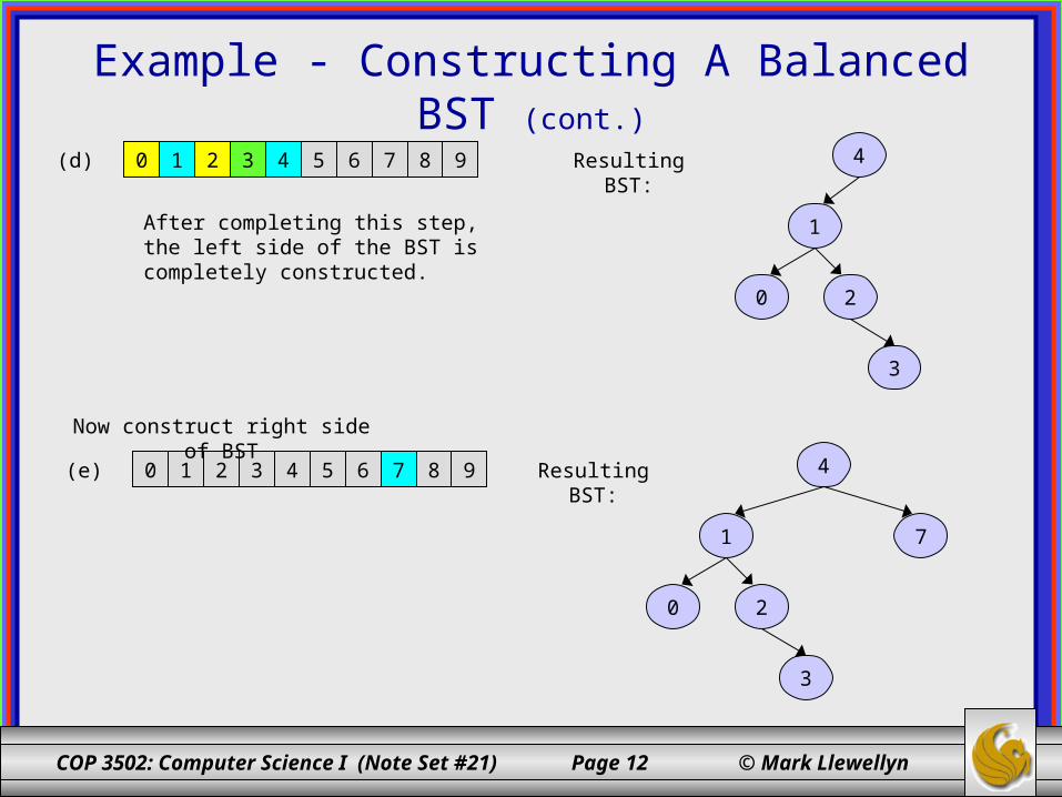
Example - Constructing A Balanced BST (cont.)
0 1 2 3 4 5 6 7 8 9(d) Resulting BST: 4
1
0 2
3
After completing this step, the left side of the BST is completely constructed.
0 1 2 3 4 5 6 7 8 9(e)
Now construct right side of BST
Resulting BST: 4
1
0 2
3
7
COP 3502: Computer Science I (Note Set #21) Page 13 © Mark Llewellyn
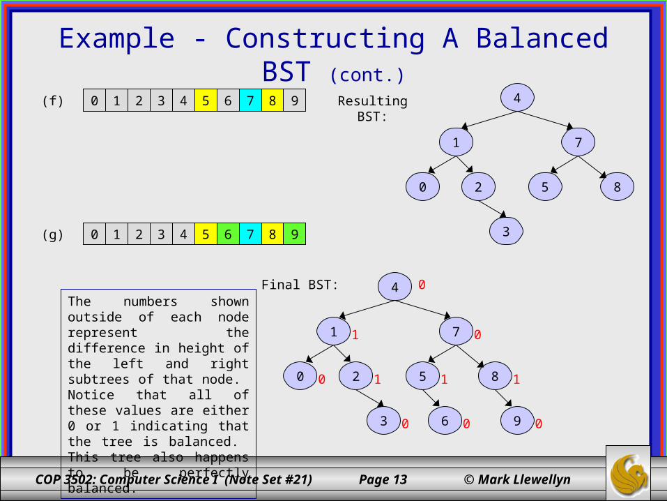
Example - Constructing A Balanced BST (cont.)
0 1 2 3 4 5 6 7 8 9(f) Resulting BST: 4
1
0 2
3
7
5 8
0 1 2 3 4 5 6 7 8 9(g)
Final BST: 4
1
0 2
3
7
5 8
6 9
The numbers shown outside of each node represent the difference in height of the left and right subtrees of that node. Notice that all of these values are either 0 or 1 indicating that the tree is balanced. This tree also happens to be perfectly balanced.
0
1
1
0 0 0
1 1
0
0

COP 3502: Computer Science I (Note Set #21) Page 14 © Mark Llewellyn
• While the previous algorithm for constructing a balanced binary search tree is certainly simple, it has one serious drawback: all the data must be put into an array before the balanced tree can be created.
• This algorithm will not work when the tree must be in use before all of the data have arrived.
• Can you think of a way to create a balanced tree from an existing unbalanced tree without requiring the data to be sorted as this algorithm requires?
– One way to do it would be to read the data from an unbalanced tree into an array using an inorder traversal of the tree. The unbalanced tree could then be destroyed and a new one created from the data in the array using the previous algorithm. In this fashion, no sort is required to put the data into order!
Problems with the Previous Algorithm
COP 3502: Computer Science I (Note Set #21) Page 15 © Mark Llewellyn
• While the previous algorithm was certainly simple, it was basically inefficient in that an additional array was required which typically required sorting before the balanced tree could be created. To avoid the sorting, required deconstructing an existing unbalanced tree and reconstructing the tree, which is quite inefficient except for very small trees (in which case their unbalanced nature is probably not a hindrance in any case).
• There are however, several algorithms which require very little additional storage for intermediate variables and use no sorting procedure. The DSW algorithm, developed by Colin Day and later improved by Quentin Stout and Bette Warren, is a very elegant algorithm which falls into this category. This is the algorithm we will examine.
Balancing Existing BSTs

COP 3502: Computer Science I (Note Set #21) Page 16 © Mark Llewellyn
• The basic building block for tree transformations in the DSW algorithm is the rotation.
• There are two types of rotations, left rotations and right rotations, which are symmetric to one another.
• The rotation of a tree occurs about its root.
• The rotation algorithms that we will look at will use the following notation to identify nodes in a tree. The node Ch identifies a child node, the node Par identifies a nodes parent and the node Gr identifies a nodes grandparent.
• In the rotations that we will examine, a rotation always rotates a child about its parent. Left children rotate to the right about the parent and right children rotate to the left about the parent.
Balancing Existing BSTs (cont.)

COP 3502: Computer Science I (Note Set #21) Page 17 © Mark Llewellyn
Right Rotations
Gr
Par
Ch
R
QP
S
Tree before right rotation occurs
Gr
Par
Ch
RQ
P
S
Tree after right rotation
COP 3502: Computer Science I (Note Set #21) Page 18 © Mark Llewellyn
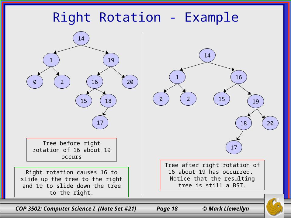
Right Rotation - Example
Tree before right rotation of 16 about 19 occurs
14
1
0 2
19
16 20
1815
17
14
1
0 2 19
16
2018
15
17
Tree after right rotation of 16 about 19 has occurred. Notice that the resulting tree is still a
BST.
Right rotation causes 16 to slide up the tree to the right and 19 to slide
down the tree to the right.

COP 3502: Computer Science I (Note Set #21) Page 19 © Mark Llewellyn
Right Rotation Algorithm
//rotate Ch about Par, Gr is grandparent of Ch, Par is parent of Ch
rotateRight (Gr, Par, Ch)
if Par is not the root of the tree //i.e., Gr is not null
grandparent Gr of child Ch becomes Ch’s parent by replacing Par;
right subtree of Ch becomes left subtree of Ch’s parent Par;
node Ch acquires Par as its right child;

COP 3502: Computer Science I (Note Set #21) Page 20 © Mark Llewellyn
Left Rotations
Gr
Par
Ch
R
Q P
S
Tree before left rotation occurs
Gr
Par
Ch
R Q
P
S
Tree after left rotation
COP 3502: Computer Science I (Note Set #21) Page 21 © Mark Llewellyn
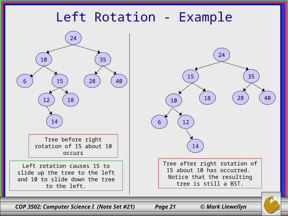
Left Rotation - Example
Tree before right rotation of 15 about 10 occurs
24
35
4028
10
156
12 18
14
24
35
402810
15
6 12
18
14
Tree after right rotation of 15 about 10 has occurred. Notice that the resulting tree is still a
BST.
Left rotation causes 15 to slide up the tree to the left and 10 to slide down
the tree to the left.
COP 3502: Computer Science I (Note Set #21) Page 22 © Mark Llewellyn
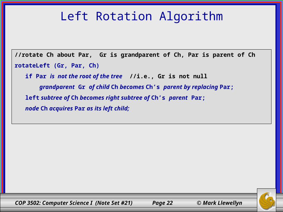
Left Rotation Algorithm
//rotate Ch about Par, Gr is grandparent of Ch, Par is parent of Ch
rotateLeft (Gr, Par, Ch)
if Par is not the root of the tree //i.e., Gr is not null
grandparent Gr of child Ch becomes Ch’s parent by replacing Par;
left subtree of Ch becomes right subtree of Ch’s parent Par;
node Ch acquires Par as its left child;

COP 3502: Computer Science I (Note Set #21) Page 23 © Mark Llewellyn
• The DSW algorithm is a two-step algorithm which results in a perfectly balanced tree.
• The first step takes an unbalanced BST and converts the tree into a backbone (sometimes called a vine). The backbone is simply an ordered linear list of the nodes that comprise the BST.
• The second step of the algorithm converts the backbone into a perfectly balanced tree by performing a series of rotations about the root of the tree. The total number of rotations that are performed is a function of the number of nodes in the tree and the resulting height of a complete tree consisting of the number of nodes in the tree.
The DSW Algorithm
COP 3502: Computer Science I (Note Set #21) Page 24 © Mark Llewellyn
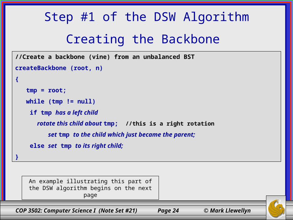
Step #1 of the DSW Algorithm
Creating the Backbone //Create a backbone (vine) from an unbalanced BST
createBackbone (root, n)
{
tmp = root;
while (tmp != null)
if tmp has a left child
rotate this child about tmp; //this is a right rotation
set tmp to the child which just became the parent;
else set tmp to its right child;
}
An example illustrating this part of the DSW algorithm begins on the next page

COP 3502: Computer Science I (Note Set #21) Page 25 © Mark Llewellyn
Creating the Backbone
10
5
23
40
20
3015
25
28
1. Initial unbalanced BST
2. First location of tmp. At this node, tmp has no left child, so it simply advances down the tree (to the right).
10
5
23
40
20
3015
25
28
tmp
COP 3502: Computer Science I (Note Set #21) Page 26 © Mark Llewellyn
Creating the Backbone (cont.)
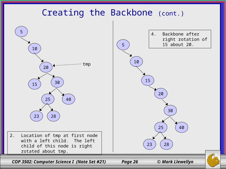
2. Location of tmp at first node with a left child. The left child of this node is right rotated about tmp.
10
5
23
40
20
3015
25
28
tmp 10
5
15
20
23
40
30
25
28
4. Backbone after right rotation of 15 about 20.

COP 3502: Computer Science I (Note Set #21) Page 27 © Mark Llewellyn
Creating the Backbone (cont.)
10
5
15
20
23
40
30
25
28
5. Next location of tmp where a left child exists.
tmp
10
5
15
20
23
40
30
25
28
6. Backbone after right rotation of 25 about 30.

COP 3502: Computer Science I (Note Set #21) Page 28 © Mark Llewellyn
Creating the Backbone (cont.)
7. Notice that tmp has not moved and yet after the previous rotation, still has a left child so another rotation about the same node (with value 25 now) occurs.
tmp
10
5
15
20
23
40
30
25
28
10
5
15
20
25
23
40
30
28
8. Tree after rotating 23 about 25.

COP 3502: Computer Science I (Note Set #21) Page 29 © Mark Llewellyn
Creating the Backbone (cont.)
tmp
10
5
15
20
25
23
40
28
30
10. Final backbone.
10
5
15
20
25
23
40
30
28
9. Final location of tmp with a left child. Will cause right rotation of 28 about 30.

COP 3502: Computer Science I (Note Set #21) Page 30 © Mark Llewellyn
• Since performing a rotation requires knowledge about the parent of tmp, an additional reference must be maintained when the algorithm is implemented.
• In the best case, the tree is already a backbone (i.e., totally right skewed) and the while loop of the algorithm will execute n times and no rotations are performed.
• In the worst case, when the root does not have a right child, the while loop will be executed 2n-1 times and n-1 rotations will be performed, where n is the number of nodes in the tree.
• Thus, the run time of the first phase of the DSW algorithm is O(n).
Analysis of Step 1 of the DSW Algorithm

COP 3502: Computer Science I (Note Set #21) Page 31 © Mark Llewellyn
• In the second phase, the backbone is transformed into a tree, but this time the tree will be perfectly balanced by having leaves only on two adjacent levels.
• In each pass down the backbone, every second node is rotated about its parent.
• One such pass decreases the size of the backbone by one-half.
• Only the first pass may not reach the end of the backbone. It is used to account for the difference between the number n of nodes in the current tree and the number 2lg(n+1)-1 of nodes in the closest complete binary tree. Thus, overflowing nodes are treated separately.
• The core (step 2) of the DSW algorithm is shown on the next slide.
Step #2 of the DSW Algorithm

COP 3502: Computer Science I (Note Set #21) Page 32 © Mark Llewellyn
Step #2 of the DSW Algorithm
Creating a Perfectly Balanced BSTcreatePerfectTree(n)
m = 2lg(n+1) -1; //n is the number of nodes in the backbone
//perform initial rotations – these are left rotations
make n-m rotations starting from the top of the backbone;
//perform remainder of necessary left rotations
while (m > 1)
m = m/2;
make m rotations starting from the top of the backbone;
An example illustrating the second part of the DSW algorithm begins on the next page

COP 3502: Computer Science I (Note Set #21) Page 33 © Mark Llewellyn
Creating the BST From the Backbone
40
10
5
15
20
25
23
28
30
1. Initial backbone. Value of n is 9. Value of m is 7 since, 2lg(n+1) -1 = 2lg(9+1) -1 = 23-1 = 7. Thus, n-m = 9-7 = 2, so 2 initial rotations are made.
10
5
15
20
25
23
28
302. BST/backbone
after first two (n-m) initial rotations are completed.
40

COP 3502: Computer Science I (Note Set #21) Page 34 © Mark Llewellyn
Creating the BST From the Backbone (cont.)
10
5
15
20
25
23
28
303. Initially the value of
m is 7. Upon entering the while loop the value of m is reset to 3 (7/2 = 3). So 3 more rotations are made. These rotated nodes are highlighted.
40
10
5 15
20
25
23
28
30
4. After performing the first of the three rotations indicated in step 3. Rotation of 20 about 10.
40
COP 3502: Computer Science I (Note Set #21) Page 35 © Mark Llewellyn
Creating the BST From the Backbone (cont.)
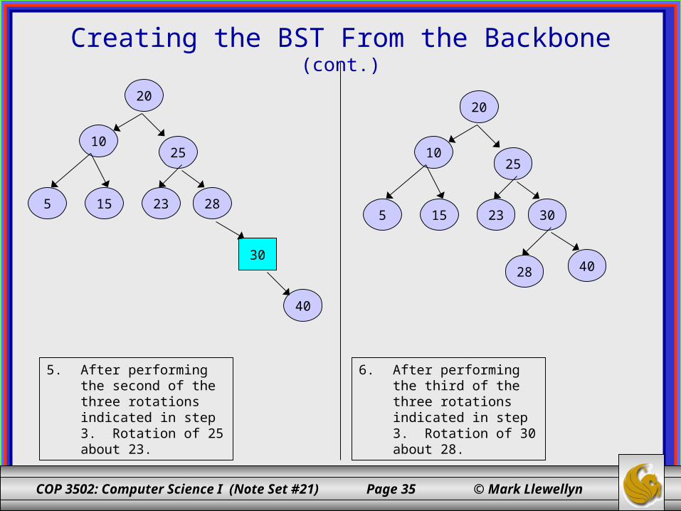
6. After performing the third of the three rotations indicated in step 3. Rotation of 30 about 28.
10
5 15
20
25
23 28
30
5. After performing the second of the three rotations indicated in step 3. Rotation of 25 about 23.
40
10
5 15
20
25
23
28
30
40
COP 3502: Computer Science I (Note Set #21) Page 36 © Mark Llewellyn
Creating the BST From the Backbone (cont.)
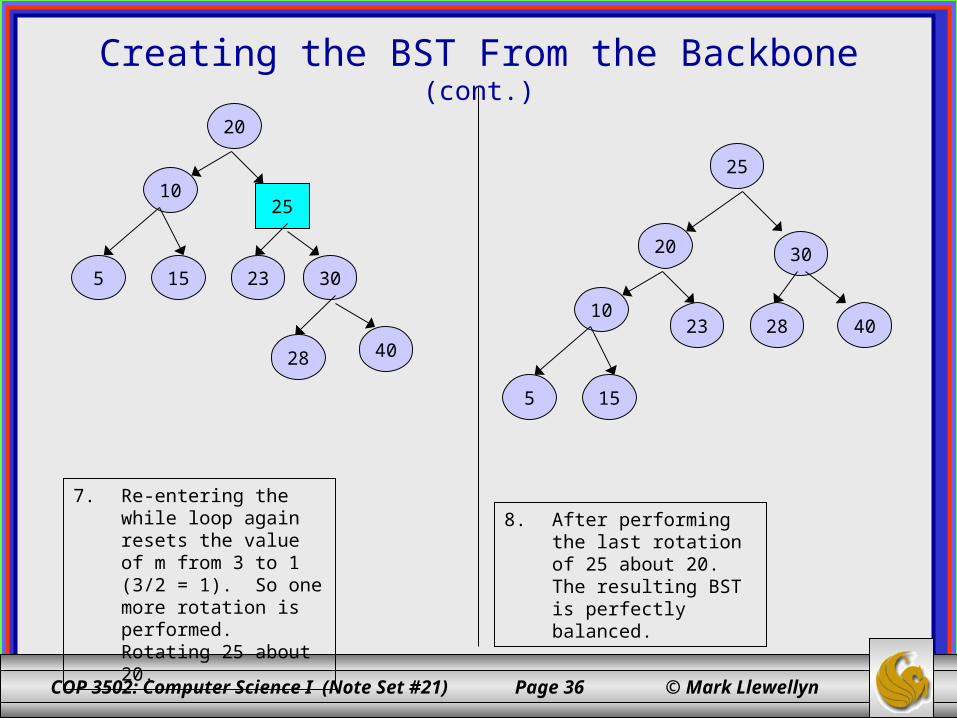
8. After performing the last rotation of 25 about 20. The resulting BST is perfectly balanced.
10
5 15
20
25
23 28
30
40
10
5 15
20
25
23
28
30
40
7. Re-entering the while loop again resets the value of m from 3 to 1 (3/2 = 1). So one more rotation is performed. Rotating 25 about 20.

COP 3502: Computer Science I (Note Set #21) Page 37 © Mark Llewellyn
• To compute the complexity of the tree building phase, note that the number of iterations performed by the while loop equals:
• The number of rotations can now be given by the expression:
• Thus, the number of rotations is O(n). Because creating a backbone also required at most O(n) rotations, the cost of global rebalancing with the DSW algorithm is optimal in terms of time because it grows linearly with n and requires a very small and fixed amount of storage.
Analysis of Step 2 of the DSW Algorithm
)lg()())lg(
)lg( 1mm12137151211m
1i
i11m
)lg(lg())lg( 1nn1mn1mmmn


![Ethio-CoP-MfDR-Concept Note June 2010 Version 2nd Draft[1]](https://img.dokumen.tips/doc/110x75/577d1e641a28ab4e1e8e6ed5/ethio-cop-mfdr-concept-note-june-2010-version-2nd-draft1.jpg)


